simulation of torsion moment at the wheel set of the railway vehicle ...

More documents

Recommendations

Info

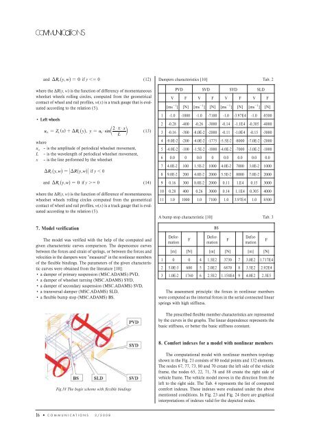
and D R _ y,wi=0 if y 0 (12) Dampers characteristics [10] Tab. 2Pwhere the ΔR(y, w) is the function of differency of momentaneouswheelset wheels rolling circles, computed from the geometricalcontact of wheel and rail profiles, w(x) is a track gauge that is evaluatedaccording to the relation (5).• Left wheels2 $ r $ xusL = Z ^ xh L + DRL _ yi, y = u0 $ sindnLwhereu o – is the amplitude of periodical wheelset movement,L – is the wavelength of periodical wheelset movement,x – is the line performed by the wheelsetDR _ y, wi=DR_y,wiLif y 0(13)and D R _ y,wi=0 if y 0 (14)where the ΔR(y, w) is the function of difference of momentaneouswheelset wheels rolling circles computed from the geometricalcontact of wheel and rail profiles, w(x) is a track gauge that is evaluatedaccording to the relation (5).7. Model verificationLThe model was verified with the help of the computed andgiven characteristic curves comparison. The depencence curvesbetween the forces and strain of springs, or between the forces andvelocities in the dampers were ”measured“ in the nonlinear membersof the flexible bindings. The parameters of the given characteristiccurves were obtained from the literature [10]:• a damper of primary suspension (MSC.ADAMS) PVD,• a damper of wheelset turning (MSC.ADAMS) SYD,• a damper of secondary suspension (MSC.ADAMS) SVD,• a transversal damper (MSC.ADAMS) SLD,• a flexible bump stop (MSC.ADAMS) BS.PVD SVD SYD SLDV F V F V F V F[ms 1 ] [N] [ms 1 ] [N] [ms 1 ] [N] [ms 1 ] [N]1 -1.0 -1000 -1.0 -7100 -1.0 -3.97E4 -1.0 -85002 -0.28 -400 -0.26 -3000 -0.14 -1.1E4 -0.305 -40003 -0.16 -300 -8.0E-2 -2000 -0.11 -1.0E4 -0.15 -30004 -9.0E-2 -200 -4.0E-2 -1775 -5.5E-2 -8000 -7.0E-2 -20005 -4.0E-2 -100 -1.5E-2 -1000 -4.0E-2 -7000 -3.0E-2 -10006 0.0 0 0.0 0 0.0 0.0 0.0 0.07 4.0E-2 100 1.5E-2 1000 4.0E-2 7000 3.0E-2 10008 9.0E-2 200 4.0E-2 2000 5.5E-2 8000 7.0E-2 20009 0.16 300 8.0E-2 2000 0.11 1.E4 0.15 300010 0.28 400 0.26 3000 0.14 1.1E4 0.305 400011 1.0 1000 1.0 7100 1.0 3.97E4 1.0 8500A bump stop characteristic [10] Tab. 3FBSThe assessment principle: the forces in nonlinear memberswere computed as the internal forces in the serial connected linearsprings with high stiffness.FDeformationDeformationDeformation[m] [N] [m] [N] [m] [N]1 0 0 4 1.5E2 3730 7 3.0E2 1.717E42 5.0E-3 600 5 2.0E2 6870 8 3.5E2 2.92E43 1.0E-2 1760 6 2.5E2 1.158E4 9 4.0E2 2.3E5FThe prescribed flexible member characteristics are representedby the curves in the graphs. The linear dependence represents thebasic stiffness, or better the basic stiffness constant.8. Comfort indexes for a model with nonlinear membersFig.18 The bogie scheme with flexible bindingsThe computational model with nonlinear members topologyshown in the Fig. 21 consists of 80 nodal points and 132 elements.The nodes 67, 77, 73, 80 and 70 create the left side of the vehicleframe, the nodes 65, 22, 71, 78 and 88 create the right side ofvehicle frame. The vehicle model moves in the direction from theleft to the right side. The Tab. 4 represents the list of computedcomfort indexes. These indexes were evaluated under the abovementioned conditions. In Fig. 23 and Fig. 24 there are graphicalinterpretations of indexes valid for the depicted nodes.16 ● COMMUNICATIONS 3/2008
Fig. 19 Forces evaluation in the damper of primary suspension(DELTA)Fig. 20 Forces evaluation in the longitudinal damper (DELTA)Fig. 21 The node points numbering in the places of indexes evaluationPassanger comfort indexes for the model Tab. 4with nonlinear membersNodeIndexfloorIndexstandingpositionNodeIndexfloorIndexstandingposition1 65 2.319 2.205 9 73 1.555 1.6922 66 2.069 2.18 10 78 1.895 2.0383 67 2.279 2.207 11 79 1.734 2.0124 22 1.707 1.763 12 80 1.872 2.045 54 1.522 1.709 13 68 2.674 2.746 77 1.692 1.737 14 69 2.49 2.7167 71 1.531 1.691 15 70 2.662 2.7428 72 1.367 1.6629. ConclusionA vehicles dynamics properties analysis is a very wide field.We can process this issue form various points of view. We put ourattention in the accelerations calculation. These accelerations inputinto the relations for passenger ride comfort assessment. The accelerationsare commonly measured in the given places of a vehiclebody when the vehicle is running. They are filtered, weighted inaccordance with the European standards ENV 12999:1999 orprENV 12999:2006 before processing for the comfort indexesevaluation [1, 12]. The accelerations in question can be obtainedwith the help of a simulation computation [5] as well. The methodof mathematical model computation, vehicle parameters andboundary conditions are of great importance for results (accelerations)trustworthiness. In the paper we described one proposalor idea of possible verification of a computational nonlinear modelbased on a strictly given mechanical system excitation which comesout from real track data. The final accelerations as the vehiclemodel response from excitation were used as input parameters forthe common comfort index evaluation due to the above mentionedEuropean standard.COMMUNICATIONS 3/2008 ●17
Page 5 and 6: Mt = k$ Di(12) 4. Torsion moment at
Page 7: References[1] JOVANOVIC, R.: Tensio
Page 10 and 11: Fig. 3 Geometrical parameters of ch
Page 12 and 13: Fig. 13 10. eigenvector when the ei
Page 16 and 17: Fig. 22 Comfort for passengers for
Page 18 and 19: 3. Intermodal trainsIntermodal trai
Page 20 and 21: Fig. 2 Consignment reloading proces
Page 22 and 23: attached to individual tracks shown
Page 24 and 25: Juraj Gerlici - Tomas Lack *MODIFIE
Page 26 and 27: After the insertion of the previous
Page 28 and 29: where:k - is the basic spring stiff
Page 30 and 31: [2] GERLICI, J., LACK, T.: Methods
Page 32 and 33: Resulting from experience the degre
Page 34 and 35: Upon this strengthening of pretensi
Page 36 and 37: attained the 6th position of the be
Page 38 and 39: Jozef Jandacka - Stefan Papucik - V
Page 40 and 41: spacing of the fan from the measuri
Page 42 and 43: 5. ConclusionFrom the results prese
Page 44 and 45: REVIEWlines with numerous curves th
Page 46 and 47: REVIEWmeters from the point of view
Page 48 and 49: REVIEWBojan Cene - Aleksandar Rados
Page 50: REVIEWthe year 2006 in Slovenia sta
Page 53 and 54: REVIEWthat the GPS does not recogni
Page 55 and 56: REVIEWRadomir Brkic - Zivoslav Adam
Page 57 and 58: REVIEWfailures. For example, for an
Page 59 and 60: REVIEWJan Krmela *COMPUTATIONAL MOD
Page 61 and 62: REVIEWFor this reason tyres and whe
Page 63 and 64: REVIEWFig. 6 Computational model
Page 65 and 66:
REVIEW- guarantee that the messages
Page 67 and 68:
REVIEWIvana Olivkova *PASSENGER INF
Page 69 and 70:
REVIEWLike the other information sy
Page 71 and 72:
REVIEWFig. 1 Revolution of the poin
Page 73 and 74:
REVIEWFig. 4 Transformation of the
Page 75 and 76:
BOOK REVIEWKavicka, A., Klima, V.,
show all

simulation of torsion moment at the wheel set of the railway vehicle ...

Create successful ePaper yourself

Delete template?

Save as template?