FOR LOWFREQUENCY SEISMOMETRY - IRIS

PROSPECTSFOR LOW-FREQUENCYSEISMOMETRYA REPORT OF THE IRIS BROADBANDSEISMOMETER WORKSHOPHeld March 24-26, 2004Granlibakken, CaliforniaEdited by S. Ingate & J. Berger

Steering CommitteeJonathan Berger, Co-Chair ......... University of California, San DiegoShane Ingate, Co-Chair .............. IRISJohn Collins .................................. Woods Hole Oceanographic InstitutionWilliam E. Farrell ........................ Science Applications International CorporationJim Fowler .................................... IRIS/PASSCAL Instrument CenterPres Herrington ........................... Sandia National LaboratoriesCharles Hutt ................................. US Geological SurveyBarbara Romanowicz .................. University of California, BerkeleySelwyn Sacks ................................ Carnegie Institution of WashingtonErhard Wieland ........................... Universität StuttgartWorkshop Presentations and DiscussionBackground material provided in advance of the workshop, and the recordof presentations and discussions may be found on the included CD and also at:http://www.iris.edu/stations/seisWorkshop04/seisWorkshop.htm

PROSPECTSFORLOW-FREQUENCYSEISMOMETRYA REPORT OF THE IRIS BROADBANDSEISMOMETER WORKSHOPHeld March 24-26, 2004Granlibakken, CaliforniaEdited by S. Ingate & J. Berger

asgjkfhklgankjhgads

ContentsExecutive Summary ....................................................................................................................... 11. Introduction ................................................................................................................................ 22. Background ................................................................................................................................. 42.1. The Seismic Spectrum .................................................................................................... 42.2. Seismic Networks ............................................................................................................ 72.3. Today’s Sensors ................................................................................................................ 82.4. Overall Criteria for the GSN Seismometers .............................................................. 103. New Ideas and Concepts ......................................................................................................... 123.1. Micro Electro Mechanical System (MEMS) Seismometer ...................................... 123.2. Electrochemical Transducer Suspension Design ...................................................... 123.3. Magnetic Levitation Seismometer .............................................................................. 123.4. Ferro-Fluid Suspension ................................................................................................ 123.5. Quartz Seismometer Suspension ................................................................................ 133.6. Folded Pendulum ..........................................................................................................133.7. Electrochemical Displacement Transducers .............................................................. 133.8. SQUID Displacement Detector ................................................................................... 133.9. Optical Displacement Transducer ............................................................................... 133.10. Superconducting Gravimeter .................................................................................... 143.11. SLAC Strainmeter ....................................................................................................... 143.12. Feasibility of Using LIGO Facilities as Strainmeters .............................................. 143.13. Ring Laser Gyro ........................................................................................................... 143.14. New Forcing and Sensing Methods for Seismometers ........................................... 143.15. Atomic Fountains for Inertial Sensors ..................................................................... 144. Testing and Test Facilities ........................................................................................................ 154.1. Introduction ................................................................................................................... 154.2. Test Facilities .................................................................................................................. 154.3. Test Procedures .............................................................................................................. 164.4. Support and Access .......................................................................................................165. Partnerships between Industry and Academia .................................................................... 175.1. Historical Background .................................................................................................. 175.2. What is an Appropriate Relationship? ........................................................................ 175.3. Respect for Intellectual Property ................................................................................. 195.4. Student Involvement ..................................................................................................... 196. Education and Funding ........................................................................................................... 207. Acknowledgements .................................................................................................................. 218. References .................................................................................................................................. 22Appendix: Workshop Attendees ................................................................................................. 23

asgjkfhklgankjhgads

Executive SummaryFor nearly a quarter of a century, the development of seismicsensors with low noise and high resolution in the normalmode frequency band (0.3-7 mHz) has languished. Theseismometer of choice for this field of seismology is now over20 years old, and is no longer being manufactured. Newersensors, albeit more portable and physically robust, more energyefficient, and less expensive, are less capable of recordingEarth motions in this frequency band. Over the same timeperiod, the training of seismic instrumentalists in departmentsof Earth science has languished; no longer do academicseismologists design and build new sensors. Outside of traditionalscience departments, however, a number of innovativeideas have been proposed for novel seismic instruments.In March 2004, IRIS sponsored a workshop on the futureof long-period seismometry, which brought together over 60participants from government, academic, and business sectorsof eight countries. Representatives of groups involved insensor technology, material sciences, and nanotechnologywere all present. The workshop’s goals were to assess emergingtechnologies that may have seismometric applicationsand formulate a plan to revitalize research and developmentof techniques in seismometry and related seismographic instrumentationin the United States.Workshop participants made several important observationsand recommendations:• The cornerstone sensor of the Global Seismographic Network(GSN), the Streckeisen STS-1, is aging and no longerin production. There are no sensors currently in productionor in development that match its performance.• Industry is unwilling to develop a substitute sensor forthis frequency band due to the anticipated unfavorablereturn on investment. (A total production run of 200units only is projected.)• Many workshop participants have come to believe thatthe goal to develop an all-purpose sensor, spanning thefrequency band from millihertz to decahertz, should beabandoned, and that two separate transducers shouldbe used to cover this range. Such a decision might easethe technological challenge and reduce the burden onindustry.• An innovative program involving academia, industry, andgovernment is recommended to nurture development ofthe next generation instruments and to educate the nextgeneration of US seismic system developers.• A program total of $10M-$20M over a period of 5-10years is envisioned.• Development needs to commence now to prevent significantdeterioration of the GSN over the next 5-10 years.1

1. IntroductionSeismology provides the only direct method for measuringthe properties of the deep interior of our planet. Seismic sensorsrange from mass-produced geophones, costing a fewhundred dollars and used by the oil industry by the thousands,to low-noise, high-sensitivity instruments that requirecareful installation in boreholes or underground vaults andcost up to $75,000 or more.Seismic sensors are the mechanical or electromechanicalassemblies that convert Earth motion into electrical signalsthat can then be digitized and recorded for later analysis.Here, sensors are distinguished from systems, in that the lattermay consist of multiple combinations of the former, coupledto a digitizing and recording apparatus.Few fundamental advances have been made in seismicsensors since the deployment of force-feedback systems near-ly a third of a century ago (see Box 1). In the intervening period,academic (and to a lesser extent industrial) research anddevelopment of seismographic instrumentation has declined.Today, adequate sensors to meet some important scientific requirementsare in short supply (see Box 2). Further, the poolof trained scientists working on seismographic instrumentationin the United States has dwindled to nearly zero.Following a brief introduction, this report summarizesdiscussions of the following workshop subjects.• Seismological Requirements• Manufacturing Issues• Testing and Testing Facilities• Partnerships between Industry and Academia• Education and Agency SupportBox 1: When Was the First Broadband Seismograph Built?Dewey and Byerly (1969) credit the Italian Cecchi with building the first recording seismograph around 1875. Thissensor recorded on a drum and may well have been the first broadband seismograph. However, it is widely acceptedthat the Gray and Milne seismograph (see right) is the first successful broadband seismograph. Between 1881-1882,Gray, Ewing, and Milne figured out how to extend the period of a seismometer to about 12 seconds (horizontal “garden-gate”suspension), thus producing a seismograph that had a flat response to Earth displacement from 12 secondsto shorter periods.However, the lineage to present broadband or very broadband sensors includes a few other branches. Von Rebeur-Paschwitz introduced continuous photographic recording with a 15-second period, which was responsible for the famousfirst recorded teleseism in 1889 (see right). One of Milne’s students in Japan, Omori in 1899, created a fairly sensitive60-second mechanical displacement seismograph that recorded some remarkable records of large teleseisms(see the front cover of this report for Omori horizontal recordings in Tokyo of the Alaska 1899 earthquake, showingone-minute period signals that are remarkable in their resemblance to modern very broadband seismograms).Wiechert introduced viscous damping in 1898. Credit for the first feedback-stabilized broadband sensor probablygoes to the remarkable 21-ton de Quervain and Piccard mechanical system at Zurich, 1926, an important developmenttowards force-balance systems. The first direct digital recording seismograph was operational at Caltecharound 1961. The Graefenberg array was the first modern digital broadband array in the late 1970s, and prompteddevelopment of the Wielandt and Streckeisen 20s STS-1. Plesinger was the first to implement a very broad velocityresponse, 0.3-300s, although the utility was hampered by analog recording available in the early 1970s. Plesinger’sresearch, however, inspired Wielandt and Steim to develop the digital VBB concept, leading in the mid 1980s to theIRIS/GSN’s 360s STS-1/VBB.2

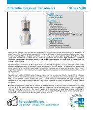
Box 2. Science Without Very Broadband SensorsWhat if the GSN consisted solely of broadband sensors (such as the STS-2)rather than very broadband sensors (such as the STS-1, which is no longerin manufacture, nor are there any plans to resume production)? Arethere any useful signals that would not be recorded? The once-in-a-lifetimeMw 9.3 Sumatran event of 12/26/04 enabled scientists to observerarely seen gravest free oscillations such as 0S 2,. These signals are rare becausesmaller sources do not generate the gravest modes with sufficientamplitude to be detected. The plot is a spectrum computed for collocatedSTS-1 and STS-2 sensors at station PFO in California. The inset boxes areenlargements of the main spectra to show amplitudes of the gravestmodes. STS-2 vertical went nonlinear on the first Rayleigh wave for thisevent, so the first surface wave arrivals were removed before spectrum estimationfor the vertical component. The STS-2 did not record the gravestmodes below 0S 3with sufficient signal –to-noise- ratio, yet the signals areeasily seen in the STS-1 spectra. Figure courtesy of J. Park, Yale University.3

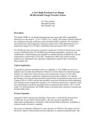
2. Background2.1. The Seismic SpectrumEarthquake-generated elastic waves that are transmittedthrough the Earth and along its surface range in frequenciesfrom less than a millihertz (the gravest eigenfrequency of thesolid Earth has a period of 54 minutes, or 0.31 mHz), to about30 Hz. Higher frequencies are attenuated so rapidly that theydo not travel appreciable distances. These five frequency decadesconstitute the seismic band; the term broadband is usedby seismologists to indicate this entire frequency band.The seismic source, whether a man-made explosion orearthquake, usually has a duration ranging from millisecondsup to a few minutes only, but the motions excited by thelargest events can last days. Although the transient seismicsignals radiated by localized sources of finite duration arecoherent with a well-defined phase spectrum, this is not thecase for ambient seismic noise. The latter is often caused by adiversity of different, spatially distributed, and often continuoussources such as wind, ocean waves, and cultural. Seismicnoise thus forms a more or less stationary stochastic processwithout a defined phase spectrum.The dynamic range of the seismic spectrum extends fromthe level of the background ambient noise to the largest signalsgenerated by seismic sources. Both limits are frequencydependant, and the signal levels are also dependant on thedistance between source and receiver. The bounds on signalsand noise are well established by observation.2.1.1. Earthquake SignalsTraveling waves from earthquakes are traditionally dividedinto three categories depending upon the source-receiverdistance. Earth’s free oscillations, or normal modes, form anothercategory. Due to the effects of internal friction, the frequencycontent of the signals also varies with source-receiverdistance. The categories are roughly described in Table 1.Figure 1 plots representative earthquake spectra recordedat local, regional, and teleseismic distances for a range ofearthquake magnitudes. To make meaningful comparisonsbetween deterministic signals and random noise, the spectralunit is root-mean-square (RMS) acceleration in frequencybands with a width of one octave.Of particular importance for long-period seismometryare Earth’s free oscillations, or normal modes. Followinglarge earthquakes, Earth’s free oscillations are observedas spectral peaks in the frequency band of 0.3-7 mHz. Thegravest mode of vibration, 0S 2, has a frequency of 0.3 mHz,and splitting of this peak is frequently observed. At higherfrequencies, the split modes overlap, and spectral resolutiondecreases. Above approximately 7 mHz, normal modes aretoo closely spaced to be resolvable, and other techniques,based on propagating wave theory, are more appropriate forthe analysis of seismograms.The development of spectral techniques for the analysisof Earth’s free oscillations was prompted by the 1960 M 9.6Chile earthquake. Over the last 40 years, the deployment ofglobal networks of sensors, together with advances in theory,have markedly improved our understanding of the average(1-D) Earth.For example, measurement of the eigenfrequencies of freeoscillations sensitive to Earth’s core has confirmed the existenceof a solid inner core (Dziewonski and Gilbert, 1971).Eigenfrequency measurements have led to the developmentof reference 1-D Earth models for elastic-wave velocities,Table 1.Category Distance Frequencies RMS AmplitudesLocal Signals up to ~30 km .3 to 30 Hz to ~ 10 ms -2Regional Signals ~ 1000 km ~10 -1 to ~10 Hz to ~10 -1 ms -2Teleseismic ~ 10,000 km ~10 -2 to ~1 Hz to ~10 -3 ms -2Normal Modes Whole Earth 3x10 -4 to ~10 -2 Hz to ~10 -5 ms -24

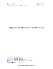
RMS Acceleration in Octave Bandwidth (ms -2 )10 010 -210 -410 -610 -810 -1010 -12STS-2 full scaleSTS-1 full scaleThe Earthquake SpectrumM8.0M7.0Sumatra-AndamanSpectrumM6.02 G AccelerometerGSN Min~3 x 10 -10 m/s10 -4 10 -3 10 -2 10 -1 10 0 10 1Frequency (Hz)M7.5M6.5M5.5M4.5M3.5180 dBM2.5M1.5M7.5M1.5Teleseismic ~3000 kmRegional ~100 kmLocal ~10 kmFigure 1. Representative earthquakespectra as recorded at various source distancesand for a range of magnitudes.The plot also compares these signal levelsto ambient Earth noise. To make meaningfulcomparisons between deterministicsignals and random noise, the spectralunit is RMS acceleration in one-octavebands. The shaded area indicates thespectral range of earthquake signals andincludes the signals from the December26, 2004 Sumatra-Andaman earthquakeobserved at the closest stations (1585km to 2685 km). The lower green line illustratesthe minimum noise observed onthe GSN stations (Berger et al., 2004). Thepink lines indicate the full-scale dynamicrange of the principal GSN sensors. Figurecourtesy of J. Berger, UCSD, after Clintonand Heaton (2002).density, and attenuation (Q) that are still widely used today(e.g., the Parameterized Reference Earth Model [PREM])(Dziewonski and Anderson, 1981). Most importantly, the littleinformation we have about Earth’s radial density structurecomes primarily from normal mode data analysis.In the last 20 years, attention has shifted to the study ofdepartures from simple spherical symmetry. The earliest indicationsthat free-oscillation data contain important informationon heterogeneities were two-fold. Buland and Gilbert(1979) first observed splitting due to lateral heterogeneityin low degree modes, in particular, in the gravest mode 0S 2.A few years later the “degree-2” geographical pattern in thefrequency shifts of fundamental spheroidal modes was discovered,which has been traced back as originating in the uppermantle transition zone (Masters et al., 1982). Anomaloussplitting of core sensitive modes was one of the key observationsin the discovery of inner-core anisotropy (Woodhouseet al., 1986).There is now renewed interest in the analysis of normalmode data. This has come with the deployment of dozens ofvery broadband seismometers along with the advent of digital,high-quality (low noise and high dynamic range) recordingat low frequencies. These advances in observational capabilityhave been coupled with advances in the theory of wavepropagation in a 3-D Earth. High-quality data have made itpossible to observe the static response to the great 1994 deepBolivia earthquake (Ekström, 1995). More accurate modesplittingmeasurements have helped put definitive constraintson the rate of relative rotation of the inner core with respectto the mantle (Laske and Masters, 1999). These improvedsplitting measurements have also been used to constraincore structure and anisotropy (e.g., Romanowicz and Breger,2000; Ishii et al., 2002)Constraints from normal modes have been used in thedevelopment of the latest generations of tomographic modelsof Earth’s mantle (e.g., Masters et al., 1996; Resovsky andRitzwoller, 1999a). These models provide unique constraintson the longest-wavelength (spherical harmonic degrees 2 and4) heterogeneity. Normal mode data are the only hope forconstraining long-wavelength lateral variations in density inthe lower mantle, the subject of recent vigorous debate (e.g.,Ishii and Tromp, 1999; Resovsky and Ritzwoller, 1999b; Ro-5

manowicz, 2001). Normal-mode constraints on the densityjump at the inner core/outer core boundary, critical for theunderstanding of core formation and dynamics, have beenreanalyzed and improved (Masters and Gubbins, 2003).There is still a wealth of information about low-degreeelastic structure, particularly odd-degree structure as well asdensity, anelastic, and anisotropic structure, to be obtainedfrom free-oscillation data. Making these discoveries requireshigh-quality, low-noise measurements at the lowest frequencies(i.e., below 0.8 mHz). Large, deep earthquakes that excitethe gravest, low angular modes sensitive to Earth’s deepestparts are rare (such as the 1994 M 8.3 Bolivia or the 2001Mw 8.4 Peru events), and each of them provides different andunique constraints due to different source depths, mechanism,and locations. These events need to be observed atmany different stations so as to allow the separation of sourceand propagation effects.Also notable is the surprising discovery, six years ago, ofEarth’s “hum”—faint fundamental mode peaks seen even inthe absence of recent earthquakes. They were first observedon the vertical component of STS-1 recordings in the periodrange 2-7 mHz (Suda et al., 1998; Tanimoto et al., 1998) andon recordings of a superconducting gravity meter in the periodrange 0.3-5 mHz (Nawa et al., 1998). The mechanismexciting this hum is still the subject of vigorous research, butthe existence of seasonal variations in the level of signal suggestsan atmospheric or oceanic origin (Tanimoto and Um,1999; Fukao et al., 2002; Ekström, 2001). Discovery of the“hum” was made by stacking many days’ recordings fromquiet stations. Recently, an array technique using the propertiesof propagating surface waves has shown promise in determiningthat a significant portion of the hum may originatein the ocean (Rhie and Romanowicz, 2004).2.1.2. Ambient NoiseThe most recent study of ambient seismic noise was a comprehensiveanalysis of a year’s worth of data from 118 GSNstations (Berger et al, 2004). The frequency range was dividedinto many bins, and noise-power histograms were developedfor each bin. The position of each station’s power in each binvaried from bin to bin. The resulting noise model is illustratedin Figure 2.Acceleration Power (dB re m 2 s -3 )-100-110-120-130-140-150-160-17050%-tile25%-tile5%-tile1%-tileFigure 2. The GSN Low-Noise Model (fromBerger, 2004). The plot shows the noisepower at the 1 st , 5 th , 25 th , and 50 th percentilesfor all GSN stations and channels. The dashcurve in the figure is the Peterson Low NoiseModel, or PLNM (Peterson, 1993). This plotshows that the Earth is even quieter at longperiods than previously thought, reinforcingthe need for a good long-period seismometerto replace the STS-1. Figure courtesy of J.Berger, UCSD.-180-190PLNM-20010 -1 10 0 10 1 10 2 10 3 10 4Period (seconds)6

2.2. Seismic NetworksThe original seismic instrumentation (see Box 1) evolvedinto a highly specialized sensor, the Streckeisen STS-1. TheSTS-1 was a very broadband device designed to take fundamentalresearch into Earth’s deep internal structure andearthquake physics to new levels of resolution, and yet remainsufficiently sensitive to also record local earthquake activitywith a fidelity approaching that of sensors specificallydesigned to monitor local activity in narrow spectral windows.The STS-1 was the ultimate sensor for probing the internalstructure of the whole Earth, representing 100 years oftechnological advances in thermally stable metallurgical andelectronics development.The primary application for the STS-1 was in global andcontinental-scale networks deployed to record large earthquakesfor studies of deep Earth structure and earthquakephysics. Two networks that do use, or intend to use, theSTS-1 are:• The Global Seismographic Network (GSN), which operatesand maintains 132 permanent stations globally.• The USArray Backbone Network, one component of thenew EarthScope program (http://www.earthscope.org).USArray is a large North American seismographic networkcurrently being constructed under NSF auspices. Itwill eventually be operated by the US Geological Survey.2.2.1. The Global Seismographic Network (GSN)The Federation of Digital Broadband Seismograph Networks(FDSN) (www.fdsn.org) is an international organization forthe exchange of data from global seismic observing systems.The Global Seismographic Network (www.iris.edu/about/GSN), operated by the IRIS Consortium and the US GeologicalSurvey, is the largest network within the FDSN. The cornerstoneof the GSN, the very broadband STS-1 seismometer,is no longer in production. The GSN is now faced with anaging technology base of equipment that cannot be replaced.Thus, unless steps are taken now to explore new and innovativetechnologies, the GSN will increasingly be unable tomeet the scientific demands of the community.GSN leadership has been aware of this problem for sometime. The following paragraphs, excerpted from “Global SeismicNetwork Design Goals Update 2002,” was prepared bythe GSN ad hoc Design Goals Subcommittee, chaired by T.Lay (http://www.iris.edu/about/GSN/docs/GSN_Design_Goals.pdf):The design of today’s Global Seismographic Network (GSN)dates back to 1985. The original design goals emphasized 20sample/sec digital recording with real-time or near real-timedata telemetry of all teleseismic ground motions (assumingabout 20 degrees station spacing) for earthquakes as large asM w= 9.5 (equivalent to the 1960 Chile earthquake) by a uniformglobal network of about 100 stations, with low noise instrumentationand environment, standardization of systemmodules, and linearity of response. These design goals wereframed within the context of both scientific goals of the researchcommunity and by general philosophy of network designand recording system attributes that service the scientific applicationsof the recorded data. The intent was for total systemnoise to be less than the ambient Earth noise over the operatingbandwidth, and to record with full fidelity and bandwidth allseismic signals above the Earth noise.Adaptation of GSN design goals to accommodate emergingscientific directions has been, and should continue to be, an ongoingprocess. However, since 1984 there has not been a community-widediscussion of scientific directions to guide or modifya future vision of GSN instrumentation. Renewal proposalsfor IRIS funding from NSF have included updated applicationsof GSN data, but there has not been a forum for broad thinkingon expanded roles or capabilities for GSN in the future. Thus,there is a general sense that, at a minimum, the existing instrumentationstrategy is serving the community rather well andthe original design criteria need to be sustained.Further, there is increasing scientific interest in ultra-longperiod signals, such as the Earth’s spectrum of continuouslyexcited modes and tides. For example, super conducting gravimetershave demonstrated superior response to existing GSNinstrumentation for very long-period free oscillations, and inclusionof a subset of these gravimeters at very quiet sites in theGSN may prove very attractive in the future. The value of highfidelity recording throughout the tidal band is not self-evident,and community discussion of the role GSN should play in datacollection at frequencies below the normal mode band (as forsome ocean oscillations) should be undertaken.7

2.2.2. USArray & EarthScopeEarthScope is a set of integrated and distributed multi-purposegeophysical instrumentation that will provide the observationaldata needed to significantly advance knowledge andunderstanding of the structure and dynamics of the NorthAmerican continent. One element of EarthScope is USArray,a dense array of high-capability seismometers that willimprove greatly our resolution of the continental lithosphereand deeper mantle.USArray’s Backbone Network serves as a reference forthe continental-scale imaging being performed by USArray’stransportable components. As an integrated resource bothfor EarthScope science and seismic monitoring, the BackboneNetwork has been designed in close collaboration withthe USGS Advanced National Seismic System (ANSS) (seewww.ANSS.org). The proposed national broadband networkcomponent of the ANSS will consist of approximately 100stations, of which USArray will contribute 9 new GSN-qualitystations and 27 ANSS-quality stations.USArray has been unable to acquire STS-1 sensors andconsequently, the Backbone has been de-scoped and will useenhanced-performance STS-2 broadband sensors instead ofthe preferred STS-1 sensors.2.2.3. Other NetworksSeismic sensors find application in a number of other fields;however, the design requirements for these systems are lessdemanding than for low-frequency sensors, and the engineeringand production challenges tend to be driven by costminimization and environmental factors (size, ruggedness,reliability). Seismic networks to monitor nearby activity requiremoderate sensitivity, but only at higher frequencies, oforder 0.1 to 10.0 Hz. Engineering seismology applicationsfocus on higher signal levels (“strong motion”) and frequenciesup to 100 Hz. Sensors for the petroleum explorationindustry must cover the band from 4 to 500 Hz, be cheap,small, rugged, and easily deployed.2.3. Today’s SensorsHistorically, seismic sensors were separated into two generalclasses: those with long (15-30 sec) and short (1 sec) free periods.The former were used to measure long-period Earthmotion such as those characteristic of surface waves, whilethe latter sensors were used to measure high-frequency Earthmotions characteristic of body waves (seismic waves thattravel through Earth’s interior). The widespread applicationof force feedback has made this distinction less importantthan in the past. More recent designs favor broadband (fromnear zero frequency to around 50 Hz) feedback instrumentsfor most applications, but the mechanical sensor can stillhave either a short free period or a long free period. However,this approach is undergoing reappraisal.Although the mass-and-spring system is a useful mathematicalmodel for a seismometer, it is incomplete as a practicaldesign. The suspension must suppress five out of the sixdegrees of freedom of the seismic mass (three translationaland three rotational) but the mass must still move as freelyas possible in the remaining direction. Furthermore, it mustsuppress the disturbing influence caused by changes in gravity,magnetic, thermal, and barometric pressure. Carefulmanufacture is essential in order to reach the Brownian limitin the motion of the suspended mass.The dynamic range of the signals to be measured is large.Figure 1 showed that an acceleration-sensitive seismometerneeds a very large dynamic range in order to resolve with fullfidelity signals ranging from those barely above the noise tothose from earthquakes of magnitude 9.5.Excellent reviews of the history of seismometer design aregiven by Melton (1981a, 1981b), Farrell (1985), and Howell(1989). The design of the so-called very broadband seismometeris well described by Wielandt and Streckeisen (1982) andWielandt and Steim (1986).Seismic sensors can be characterized by their frequencyresponse, sensitivity, self-noise, and dynamic range.2.3.1. Frequency ResponseToday’s seismometers can be divided into three rough categories.Figure 3 shows the frequency response of a numberof seismic sensors.Short-period (SP) seismometers and geophones measuresignals from approximately 0.1 to 250 Hz, with lower cornerfrequencies between 1 and 10 Hz. Their response is usuallyflat with respect to ground velocity above this corner frequency.These units are technically simple and are readily available.High-quality units without significant parasitic resonance costaround $6,000; geophones cost a few hundred dollars.8

Figure 3. Frequency response of representative seismometers. Figure courtesy of R. Hutt, USGS/ASL.Broadband sensors (BB) have a response shifted down infrequency by about two decades with respect to SP sensors.Usually, their transfer function is flat to velocity from approximately0.01 to 50 Hz. Sensors in this class are also readilyavailable, though they are somewhat more expensive (typically$15,000). They are fragile and require relatively highpower (~0.5 W or more).So-called very broadband seismometers measure groundmotion at frequencies from below 0.001 Hz to approximately10 Hz and are able to resolve Earth’s tides. They are extremelyfragile and high power consumers (~several watts). They areexpensive (typically $45,000 for a surface sensor, $100,000 fora borehole sensor and installation).2.3.2. SensitivitySeismometers are weak-motion sensors, usually orders ofmagnitude more sensitive than accelerometers, though theycannot record as large amplitudes as accelerometers. Seismometerscan record local but small events and/or large butdistant events. The goal for a VBB seismometer is to measureground motion smaller than the amplitudes of the lowestnatural seismic noise found anywhere in the world.Accelerometers are strong-motion sensors, and in geophysicaland earthquake engineering applications, measureseismic signals between near-DC to up to 50 Hz. However,output voltage of an accelerometer is proportional to groundacceleration, whereas seismometer output is generally pro-9

portional to ground velocity. For this reason, accelerometersstress high frequencies and attenuate low frequencies comparedwith seismometers.2.3.3. Self-noiseAll modern seismographs use semiconductor amplifiersthat, like other active (power-dissipating) electronic components,produce continuous electronic noise whose originsare manifold but ultimately related to the quantization of theelectric charge. The contributions from semiconductor noiseand resistor noise are often comparable, and together limitthe sensitivity of the system. Another source of continuousnoise, the Brownian (thermal) motion of the seismic mass,may be noticeable when the mass is very small (less than afew grams). Seismographs may also suffer from transient disturbancesoriginating in slightly defective semiconductors orin the mechanical parts of the seismometer when these aresubject to stresses. An important goal in constructing a verybroadband sensor for Earth studies is for the self-noise to beconsiderably less than the lowest ambient Earth noise. TheGSN Low-Noise Model (Figure 2) summarizes the observedseismic noise levels throughout the seismic frequency band.This model is useful as a reference for assessing the quality ofseismic stations, for predicting the presence of small signals,and for the design of seismic sensors.Comparing self-noise of very broadband and broadbandseismometers is instructive. The very broadband STS-1 seismometerhas a theoretical noise of around 4 x 10 -11 m/s 2 /√Hzat a period of around 8 sec, and 5 x 10 -10 m/s 2 /√Hz at 1000sec. The broadband STS-2 can achieve a noise level of 2.5 x10 -9 m/s 2 /√Hz at 1000 sec.2.3.4. Dynamic rangeIn a conventional passive seismometer, the inertial force producedby a seismic ground motion deflects the mass from itsequilibrium position, and the displacement or velocity of themass is then converted into an electric signal. This classicalmechanism is now used for short-period seismometers only.Broadband seismometers usually are of a force-feedback design,which provides greater linearity but sometimes at theexpense of reduced dynamic range. Here, the inertial force iscompensated (or “balanced”) with the electrically generatedforce required to constrain the seismic mass. The feedbackforce is generated with an electromagnetic force transducer.Due to unavoidable delays in the feedback loop, force-balancesystems have a limited bandwidth; however, at frequencieswhere they are effective, they force the mass to movewith the ground by generating a feedback force strictly proportionalto ground acceleration. When the force is proportionalto the current in the transducer, then the current, thevoltage across the feedback resistor, and the output voltageare all proportional to ground acceleration. Thus, accelerationcan be converted into an electric signal without dependingon the precision of the mechanical suspension.2.4. Overall Criteria for the GSNSeismometersA characterization of current seismological instrumentationcapabilities is shown in Figures 1, 2, and 3. A combinationof sensors is often used to realize a full response, and ifadvances in sensor design can achieve greater performance(while retaining linearity, resolution, bandwidth, and dynamicrange) over the full seismic spectrum, it would be attractiveto incorporate such instrumentation into the GSNin the future. The GSN design goal is to achieve at least thebandwidth and dynamic range indicated in these figures, as ispresently achieved by the current optimal GSN instrumentation.This should guide the development of instrumentationspecifications for all future GSN instrumentation.Table 2 was excerpted from the 2002 GSN ad hoc DesignGoals Subcommittee document (www.iris.edu/about/GSN/docs/GSN_Design_Goals.pdf), indicating the functionalspecification goals of the next-generation GSN sensor. Thefunctional specifications are derived from the design goals byconsidering detailed limits of the general scientific goals. Ingeneral, it’s worth making the instrumentation about an orderof magnitude better than our ability to model the parametersbeing measured. Thus, if it is intended to model amplitudesto 20%, the aggregate sources of amplitude error (gainstability, cross-axis coupling, and cross talk) should be lessthan 2% and individual contributions should be even less.10

Table 2. GSN Sensor Requirements.Dynamic rangeClip levelSelf-noiseLinearityBandwidthCalibrationCross-axis couplingDegrees of freedomReliabilityShock and vibrationOther environmentalOn-scale broadband recordings of earthquakes as large as Mw = 9.5 (equivalent to the 1960 Chileearthquake) at 4,500 km.5.8 m/s RMS over the band 10 -4 seconds (or below) to 15 Hz.Below ambient Earth noise.Total harmonic distortion < 80 dB at 50% maximum acceleration and frequencies within the passbandof the feedback loop.Earth free oscillations to regional body waves (up to 15 Hz for land stations, 100 Hz for ocean-bottomsites).Known to 1% and stable across the bandwidth (adequate for amplitude modeling which at best isgood to about 20%).Less than about 1% (adequate for amplitude modeling).Three mutually orthogonal components of motion should be recorded.MTBF of years.Equipment must be robust to survive shipping and installation.Environmental susceptibility (to temperature, pressure, magnetic fields, electromagnetic and audiofields, etc.) should not constrain site selection or deployment technique.11

3. New Ideas and ConceptsThis section summarizes emerging designs and conceptsfor very broadband seismometers that were presented at theworkshop. Abstracts, presentations, and posters are given infull in the accompanying CD.Engineering challenges for seismic sensor design arelargely noise floor, dynamic range, and stability. Two fundamentallimits in achieving a low noise floor are: (1) suspensionnoise caused by the Brownian motion of the suspendedmass, and (2) Johnson, or thermal, noise. The overview ofemerging technologies given below shows that it will be acomplex, but not overwhelming, challenge to meet or exceedthe noise floor of the STS-1 sensor.It is unclear which of the technologies behind these sensors,if any, are most appropriate for the development of anew GSN seismometer. The geoscience community alone isnot in a position to adequately assess the suitability of theseemerging technologies. It is these advances and their possibleapplication to the design of the next-generation GSN seismometerthat participants explored in the workshop.3.1. Micro Electro Mechanical System(MEMS) SeismometerDevelopments in miniaturization of broadband sensorshave reached designs achieving broadband noise levels ofaround 3 x 10 -9 m/s 2 /√Hz (compared with STS-1 and STS-2seismometers in section 2.3.3) and full-scale acceleration ofaround 2 m/s 2 in small packages (2 cm x 2 cm) weighing 1kg or less. Size reductions have come through shrinkage ofconventional spring-mass systems. This reduction is carriedout by micromachining the entire system into a “chip-based”package of a few grams using high-sensitivity piezoelectricmaterials. Some sensors are internal to the sigma-delta converterand serve as the summing junction, producing digitaldata. These miniature, small-mass sensors require veryhigh-Qsuspensions and relatively low natural frequencies toachieve suitable noise characteristics for GSN-style applications.It appears that Q values of 1000-10000 can be reachedand maintained in 10-Hz suspension systems. At present,MEMS do not provide a force-feedback mechanism, whichmay limit their dynamic range.3.2. Electrochemical TransducerSuspension DesignUnlike a traditional mass-on-a-spring seismometer design,Molecular Electronic Transfer (MET) seismic sensors haveelastic membranes instead of springs, and a significant part(or even all) of the inertial mass is liquid. The output of thesesensors is inherently independent of the inertial mass position,so no mass locks or mass centering is required. Anotherfeature of a mass-position-independent output is the simplifiedforce-balanced feedback circuit design that contains nointegrators, thus is a lower-noise operation at long periods.Current designs have a natural frequency of about 3 Hz thatallows for a velocity-flat response from 120 sec to 50 Hz.There is no theoretical limitation for expansion of the passbandto at least 1000 sec, but it will require a special, very“soft” membrane design.3.3. Magnetic Levitation SeismometerTo remove a pendulum’s high-frequency noise that resultsfrom the parasitic resonances of a suspension spring, andto reduce the thermal dependence of the spring, permanentmagnet levitation for a pendulum weight may be employed.Current implementations of this technology achieve noiselevels in a vertical-component seismometer near 10 -9 m/s 2 /√Hz near 1 Hz. Such systems have been shown to be extremelysensitive to barometric effects, necessitating installationwithin a pressure chamber. Isolated in this manner, thesesensors may demonstrate noise levels similar to that of anSTS-2 sensor.3.4. Ferro-Fluid SuspensionThe unique feature of this design is that it makes use of asuspended magnetic mass to measure ground velocity (i.e.,it does not make use of springs or noise-producing mountingsuspensions). Positioning a permanent rod magnet withina cylindrical cavity containing a ferromagnetic fluid is africtionless and noiseless way to configure a velocity sensorproof mass. Positioning a coil around the housing is an easyway to measure the velocity of the case. In addition, this implementationprovides for very large deployment forces with-12

out changing the characteristics of the device. The potentialto force-balance the proof mass offers even greater low-frequencyperformance.3.5. Quartz Seismometer SuspensionThe proposed 1 TeV X-band electron/positron linear colliderat SLAC (Stanford Linear Accelerator Center) will producebeams with approximately 1 nanometer vertical sizes at thecollision point. The final focusing magnets for this acceleratormust be held at the nanometer level relative to each other.Beam-beam interactions provide a signal for a high gainfeedback for frequencies below ~1 Hz, but additional stabilizationis required at higher frequencies. One option is to useinertial sensors (geophones) to provide a feedback signal. Thehigh magnetic fields mean that the seismometer must not besensitive to magnetic fields, preventing the use of temperature-compensatedspring materials, and so a novel quartzsuspension system was develeoped. Temperature variationsprobably are a major noise source below 0.1 Hz. Preliminarytesting against a STS-2 sensor shows that the noise floor isbelow 10 -8 m/s 2 /√Hz, and that the 1/f noise corner is ~0.1 Hz.3.6. Folded PendulumFolded pendulums are classical suspension systems first developedmore than a century ago. Their modern developmentis partly related to gravity wave research. These systemsare too large to fit into the limited space of boreholesand seafloor packages, basically because of the compromisebetween the residual elasticity and the suspended load. Recentprogress in precision micro-machining allows extremelysoft flexures at the pendulum’s hinges. A broadband foldedpendulum with reasonable size and natural frequencies(< 1 Hz) has already been developed and tested for gravitationalwave-detection experiments. Additionally, studies ofthe flexures involved finite-element modeling to suppresstheir elasticity. As a result, it may be possible to fabricatefolded pendulums with dimensions on the order of a fewcentimeters, which is required for borehole and seafloorseismic sensor applications.3.7. Electrochemical DisplacementTransducersMET technology features an innovative transducer designsuitable for low-noise translational and rotational seismicsensors. The transducer consumes extremely small amountsof power (down to 30-50 mW), has a very low self-noiselevel, and is insensitive to strong magnetic fields. MET transducersconsist of four microscopically thin platinum meshelectrodes separated by thin-film microporous spacers placedin a tube filled with an iodine-based electrolyte. A small DCoffsetis applied between each pair of electrodes. The convectivediffusion phenomenon is used to convert the flow ofthe electrolyte to the electric current. This transducer has asymmetric configuration and a differential output that allowsfor linear operation with 120-130 dB dynamic range. Withforce-balanced feedback (electrodynamic or magneto-hydrodynamictype), dynamic range can be extended to 150-160dB. The electrochemical transducer features an accelerationflatnoise power spectral density that is determined by itshydraulic impedance (similar to Nyquist noise of a resistor).In a 2-inch diameter rotational sensor, noise spectral densityis about 3 x 10 -7 rad/s 2 /√Hz. Translational sensors havenoise levels below 3 x 10 -9 m/s 2 /√Hz. Lower noise levels canbe achieved by development of a lower hydraulic impedanceelectrochemical transducer.3.8. SQUID Displacement DetectorSuperconducting Quantum Interference Devices (SQUIDs)are intrinsically quieter than room-temperature displacementsensors due to material property improvement that temperaturesbelow 10 K can provide, providing theoretical limits assmall as two orders of magnitude lower than capacitive detection.To date, no seismic sensors have been constructedusing this technology.3.9. Optical Displacement TransducerThe laser interferometric displacement sensor has several advantagessuch as high resolution, low drift, low heating, andin situ calibration with reference to the wavelength of light. Awideband seismometer using a Michelson interferometer anda long-period pendulum has been developed by Japan’s EarthquakeResearch Insitute ERI. This seismometer has a selfnoiselevel below NLNM at 50 mHz to 100 Hz and has 1%in situ calibration accuracy. The optical-fiber-linked version,which may be used in high-temperature environment such asdeep borehole, is under development. Scientists at Scripps Institutionof Oceanography developed a wideband optical seismometerwith an STS-1 pendulum and a bi-directional inter-13

ferometer, and successfully operated it with a phase decodingsystem using digital signal processing. Another approach fora horizontal seismometer is a long-baseline laser strainmeterthat is essentially insensitive to local ground tilt. Although itslarge scale makes it difficult to spread into many observatories,a significant self-noise improvement of horizontal seismicobservation would be possible if a highly frequency-stabilizedlaser is used. A 100-m laser strainmeter installed inKamioka Mine (Japan, 1000 m underground) attained an effectivebackground noise level of 1 x 10 -9 m/s 2 /√Hz at 10 mHzand 4 x 10 -9 m/s 2 /√Hz at 0.5 mHz.3.10. Superconducting GravimeterSeveral superconducting gravimeters (SCG) operating in theGlobal Geodynamics Project network demonstrate lowernoise levels than the STS-1 for frequencies below 1 mHz. Increasingthe mass from about 6 g (2.5-cm diameter) to 80 g(5-cm diameter) will decrease Brownian noise by at least afactor of 100 and will be well below the NLNM for frequenciesin the normal-mode band. Current versions of the gravimeterare made in small quantities and sell for $350,000. Itis possible that versions optimized for seismology could bemanufactured for about $100,000 if quantities ordered wereroughly five per year. It was noted at the workshop that theSCG can record vertical ground motion only.3.11. SLAC StrainmeterSLAC has a 2-mile-long linear accelerator (linac) that wasbuilt about 30 years ago. The alignment system of this acceleratorconsists of a “light pipe,” which is a 60-cm diameter,2-mile-long straight evacuated pipe, with the laser source(shining through a pinhole) and a quadrant photo-detectorlocated at opposite ends. About 200 remotely controlledFresnel lenses are located along the linac, and can be insertedinto the pipe one by one. Such a system can detect lateralEarth deformation over distances of 3 km, with a resolutionof around 20 nm.3.12. Feasibility of Using LIGO Facilitiesas StrainmetersAt the LIGO Gravity-Wave Observatory sites at Hanford, WAand Livingston, LA there are sensitive laser interferometersthat monitor the distance in a vacuum between pairs of suspendedtest masses 4 km apart in two perpendicular directions,in terms of the wavelength of light from an NdYAG laser.This laser is stabilized to a reference cavity whose lengthis modulated slightly by adjusting its temperature to partiallycompensate for the changes in the 4-km baselines arisingfrom Earth tides. To use one of these interferometers to monitorEarth strain with the highest possible precision wouldrequire some additional equipment: one sensor to referencethe position of each suspended test mass to some point in theground, and another to continuously monitor and record theslowly varying frequency of the light from the NdYAG laser.Such systems may be non-trivial, though simpler compromisesolutions with lower precision are possible.3.13. Ring Laser GyroIn 2000, a joint New Zealand-German program obtainedvery encouraging results in measuring angular rates of deformationwithin the Earth’s crust. Located in a vault inChristchurch, NZ a block of low CTE (coefficient of thermalexpansion) material about 1 meter square, implemented asa ring laser gyro, has achieved a level of sensitivity that appearsto be detecting tilt due to tides. A second gyro has beeninstalled at the Piñion Flat Observatory in California by theGerman group. This technology may provide the orientationinformation needed to separate the tilt-horizontal couplingthat limits interpretation of horizontal seismometer data.3.14. New Forcing and Sensing Methodsfor SeismometersNew sensing and forcing schemes should be investigated forseismometers. Techniques that use over-sampling (256 timesor more), correlated double sampling, and fully differentialcircuits can cancel or greatly reduce sensing noise at low frequencies.Similar techniques could be applied to forcing circuitsto reduce noise in the feedback loop.3.15. Atomic Fountains for InertialSensorsAtomic fountains receive their name because atoms arelaunched upwards and fall back under gravity. Such fountainsdemonstrate an accuracy of around 10 -9 m/s 2 as a gravitymeter. Stanford is leading a development effort for a familyof inertial instruments based on this technology for field applicationin inertial navigation and gradiometry. The technologyis currently being developed at ESA for orbital flight fora science experiment of unusual sensitivity. Properly scaled,this technology has promise for geophysical measurements.14

4. Testing and Test Facilities4.1. IntroductionThe Testing & Testing Facilities (T&TF) Breakout Group begandiscussions by reviewing the highlights of discussionsof a small group that met in 1989 at the USGS AlbuquerqueSeismological Laboratory to discuss Standards for SeismometerTesting (SST) in order to compare short period,broadband, and very broadband seismic sensors. Resultsand minutes of this meeting were presented at the 1990 AnnualMeeting of the Seismological Society of America, and atsubsequent IUGG meetings and IRIS meetings (Hutt, 1990).Building upon the SST results, the Testing & Testing FacilitiesBreakout Group suggested that “Standard Parameters andStandards for Reporting Measured Parameters of VBB Sensors”were needed for users of seismic data.The group also expressed the need to identify differentkinds of tests. For example, manufacturers have specific teststhat they use in research and development and in productiontesting and certification. The suite of tests used by manufacturersmay be different from the suite of tests used for acceptancetesting by the purchasers of the sensors. The station orsystem operators may have yet a different suite of tests thatthey prefer or need after the GSN sensors are installed andoperating.Some relevant tests for GSN sensors were discussed bythe T&TF Breakout Group, and the results of the 1989 SSTmeeting were discussed in the context of defining parametersthat might need to be measured and the frequency ofre-measuring these parameters after installation and operationof the GSN sensors. The T&TF Breakout Group has tworecommendations:1. Establish a working group (or standing committee) similarin composition to the group included in the 1989SST meeting in Albuquerque and in the T&TF BreakoutGroup at Granlibakken.2. Upgrade an existing testing facility with support for instrumentationand staff that could provide a needed serviceto the GSN user community.Together, the GSN sensor working group, testing facility,and staff should provide standard parameters and measurementsof GSN sensors for the manufacturers, developers, andusers of GSN sensors and data.4.2. Test FacilitiesAdequate testing of sensitive seismometers must be performed,in part, at remote field facilities. The two premiersites for seismometer testing in the US are the UCSD PiñonFlat Observatory in California, and the USGS AlbuquerqueSeismological Laboratory in New Mexico. They meet most ofthe desiderata for high-accuracy testing including experienceand technician support, infrastructure (e.g., buildings, isolatedpillars, electricity, laboratory space, Internet access), lowenoughseismic noise, accessibility, and suitable referenceinstrumentation. At both sites the ambient noise is many dBhigher than the global minimums, but with pairs of comparableinstruments, cross-spectrum analysis can pick out thesensor noise if enough data are recorded. These two facilitieshave been sporadically improved over many years. New requirementsfor next-generation instruments may require furtherdevelopment. This might include data-acquisition equipment,additional vaults/pillars, isolation tables, calibrationtables, and environmental chambers.Other test facilities are established and fulfill a numberof purposes, but their use should not supplant some level oftesting at the premier facilities noted above. Among thesesecondary sites are the FACT site of Sandia National Laboratoriesat Kirtland Air Force Base, New Mexico and the PinedaleSeismic Research Facility at the Air Force Tactical AnalysisCenter in Wyoming. Most manufactures have seismometertest facilities (e.g., Nanometrics in Canada, and Guralpin England). Overseas academic facilities of note include theBlack Forest Observatory in Germany, the Conrad Observatoryin Austria, and an accelerometer test facility related togravity-wave detectors in Florence, Italy.15

4.3. Test ProceduresTest procedures and the method of reporting test resultsshould consider the procedures and templates describedin ANSI (2003). Many of the sections are as applicable toseismometers as they are to accelerometers for inertial guidancesystems. The Albuquerque Seismological Laboratorydocumented their approach some years ago (Hutt, 1990),and it would be appropriate to review and update these writtenguidelines. A revision should consider all phases of testing,including development testing, design qualification testing,acceptance testing, operational testing, and post-installationtesting.4.4. Support and AccessTop-notch field facilities are not cheap. As national resourcesthey should be funded, not only for the manager’s parochialinterests, but also for use of the whole community— academicand commercial, national, and international. Thus, managersshould be accommodating to all potential users andprovide visitors a range of support. However, there must bean understanding of the limits of default support, and provisionmade for recharge to handle exceptionally long or arduousvisits.In general, open circulation of test results, including peerreviewpublication, is to be encouraged. However, vendorsmay have proprietary interests in test results, whether favorableor unfavorable, and these concerns about intellectualproperty (IP) will need to be respected.16

5. Partnerships Between Industryand Academia5.1. Historical BackgroundEffective partnerships between industry and academia havegiven Earth scientists their best instruments for low-frequencyseismology. The LaCoste-Romberg gravity meter, onwhich Earth’s free oscillations were first observed, grew froma graduate student thesis into a major geophysical corporation.The superconducting gravity meter was first developedin an academic department and later commercialized. Butthese two examples are decades old, and there are no recentinstances in the United States of connections between industryand academia for development of sensors suitable forlow-frequency seismology. This is not the case in Europe,where both the Guralp and Streckeisen companies have theirroots in university research.By far the most significant work in the United States overthe last half century on seismic sensors has been directed towardsystems for nuclear test detection. These were superbfor the need, and some systems or sub-systems developedfor nuclear monitoring have been deployed in the GlobalSeismographic Network. However, it is clear that these sensorsare not the best at the lowest frequencies. Furthermore,test-detection programs ceased developing new sensors morethan a decade ago.We believe the collaboration in the United States betweenindustry and academia for developing novel seismicsensors needs to be revitalized. This collaboration shouldbe shaped by realizing that exciting discoveries in low-frequencyseismology are more likely to come from large-scaledeployments of quantities of sensors than from highly sophisticated,but one-off systems. Industry, rather than theacademic research department, is the place to manufacturecommodity instruments.Researchers will get the instruments they need only ifeach side understands the requirements and limitations ofthe other. Industry must see an opportunity for profit. Academicsseek new knowledge, and almost always, their science-basedresearch is advanced by new instrumentation. Adeep understanding of the capabilities and limitations of instrumentationis fundamental to progress.5.2. What is an AppropriateRelationship?The market for long-period sensors is so small, and the unitsthat can be sold per year so limited, that industry can not beexpected to perform the necessary R&D for this communityon speculation. This situation does not apply for instrumentsin higher-frequency bands. In the oil business, the marketcan justify investment of many millions by sensor manufacturers,because, if successful, they will sell many thousands ofunits a year. In the smaller community of body wave seismology,it is also true that manufacturers have been able to fundresearch and development internally, even for sales of a fewhundred units a year or less.In the low-frequency seismology community, we generallyrequire quantities of a few score, at most, to be deliveredover many years. This combination of market size and productionrate means that our most important task is for industryand academia to work together to obtain the R&D fundsnecessary for progress.For some years there has been the hope that an instrumenttargeted to the higher-frequency market (frequencies> .01 Hz, say) would, almost as a side effect, have adequateperformance at the very lowest frequencies. Experience hasshown that this is generally not the case. The very best lowfrequencysensors are purposely designed. Thus:• Superior low-frequency seismic sensors are not likely tobe developed from R&D funds internally generated bymanufacturers.Thus, the foundation of the academic/industrial partnershipwill continue to be an academic evangelist with a compellingscience question whose answer requires state-of-the artinstrumentation. This person is someone who is obsessedby the science, is successful at fund raising, sits on the rightcommittees, and is viewed as a dynamo in their field. They17

provide the scientific basis and enthusiasm that will be usedto motivate support from the funding agencies.The process of cooperative instrument development betweenindustry and academia begins with the conceptual designand continues through prototype production into testing.As previously noted, the academic member of this teamis responsible for the science while the industrial partnerhas the manufacturing plant. Ideally, they collaborate on thecommon ground of instrument design. This delineation isblurred in actuality, for one hopes both partners are involvedto some extent in all aspects.The following paragraphs list three activities that canjointly involve academics and industry. For each activity wedefine the contribution of each partner, and the benefit of thecontribution to the other partner.Activity: Development of New Sensor ConceptsNew sensors might be based on traditional electro-mechanicalconcepts, or involve novel technologies, including micromachiningand application of atomic and quantum physics.Academic Contribution and Benefit to IndustryConcepts can arise in departments of Earth Science or otheracademic departments, and then brought to industry.Benefit to industry:• New, marketable instrumentation ideas.• Academic laboratories a source of employees with instrumentationexperience.Industrial Contribution and Benefit to AcademeConcepts can arise internally. Academics can be involved asconsultants, or non-commercial ideas handed over undersuitable condition.Benefit to academe:• Exposure of faculty and students to industry practice.• Access to engineering support, e.g. machining, electronicdesign, prototypes.Activity: Field Testing of Sensor PrototypesTesting of sensitive instruments must be conducted in lownoisesettings, preferably with simultaneous recording of referencesensors and environmental conditions.Academic Contribution and Benefit to IndustryField observatories, especially observatories in low-noise settingsand with diverse instruments and digital data acquisitionsystems.Benefit to industry:• The best field observatories have a level of infrastructuresupport greater than industry can afford.• Ability to cross-correlate data from new sensors with datafrom other seismic and environmental sensors.• Experience of academic team in multichannel data processing.• Operation of instruments by third party under realisticfield conditions.• Independent verification of instrument performance.• Feedback from academic community for improved instruments.Industrial Contribution and Benefit to AcademeLoan of prototype or pre-production sensors for operationand evaluation.Benefit to academe:• Early familiarity with novel instruments.• Ability to influence sensor design and performance.• Challenging projects for students.• Possible financial support while conducting evaluations.Activity: Sponsorship of Research ParksUniversity administrators are increasingly interested in fosteringthe migration of research results into commercial enterprises.Research parks are incubators of startups.Academic Contribution and Benefit to IndustrySeveral universities have established research parks as incubatorsfor new businesses. Among those with notable departmentsin the Earth Sciences are: Stanford University,University of Colorado at Boulder; University of Texas atDallas, and New Mexico Tech. An example from overseas isthe University of Reading in the UK.Benefit to industry:• Continuing relationship with host university.• Availability of business-related consultants and supportservices (management, accounting, legal).• Availability of technical support services (software, hardware,mechanical).• Reduced risk through possible cost sharing with university.• Royalties and jobs for graduates if the venture is successful.Industrial Contribution and Benefit to AcademeRoyalties and jobs for graduates if the venture is successful.18

Benefit to academe:• Endowment.• Jobs and growth.• Continuing relationship with industry.5.3. Respect for Intellectual PropertyIt is important that intellectual property rights be settled beforecollaboration begins. Industry will be secretive abouttheir most valuable ideas. Academics will focus on open discourseand publication in peer-reviewed journals. Finally,university administrators are increasingly eager to protectand promote the discoveries of their faculty for financial return.This three-way tension requires careful delineation ofthese issues early in the cooperative process.The following are the principal mechanisms for protectingintellectual property. (For more information, go to http://law.freeadvice.com/intellectual_property/)• Patents: Patenting is a costly and lengthy process. A technologythat is patentable may, in fact, become obsoletebefore a patent is issued. For these reasons, this industrytends not to patent inventions in this technology. However,if an idea is patentable, the rule must be patent beforepublish.• Trade Secrets: This broad category includes almost anythingof economic value. Industry can be expected to forbidpublication of trade secrets.• Licensing Agreements: Licensing agreements allow oneparty to use, and possibly market, intellectual propertyof another party. They can work both ways: universitiescan license discoveries of faculty and staff to industry forcommercial use; industry can license intellectual propertyto academics for non-commercial research. However, inthe latter case, a non-disclosure agreement might be moreappropriate.• Non-disclosure Agreements: Non-disclosure agreementsare used by the owner of intellectual property to discloseinformation to a second party for their exclusive use.• Contracts: In the case where industry contracts withan academic for some research or development activity,the intellectual property issues would be included in theterms and conditions.The foundation of the university is the discovery and exchangeof knowledge. This exchange may indeed be advantageousto both groups as it accelerates progress and providesnew scientific and economic opportunities that each groupis free to explore on their own. If the market for some productis small, an open relationship between industry and academiacan provide a solution that benefits both parties. Therecent development of the unique “Texan” seismic recorder,developed jointly by the University of Texas, El Paso and RefractionTechnology, is an example of such an open cooperation.These sorts of exchanges can lead to additional ideas forproduct development. The success of such projects benefitsfrom the acceptance of risk and the sharing of cost by bothindustry and academia.5.4. Student InvolvementStudent training is one of the strongest reasons for industryand academia to cooperate. Historically, industry has sponsoredscholarships, intern programs, and cooperative projectsin order to support students at the interface betweenacademia and industry. Although the numbers and types ofthese programs have decreased in recent years, it is recognizedthat they need to be maintained and possibly extended.Student support by industry provides industry withyoung and energetic resources. These students can bringseismological expertise to industry under close cooperation.They also provide a resource to industry for future employment.Industry provides engineering, design, and manufacturingexperience to the student, thus providing them witha broader understanding of practical issues associated withinstrumentation.This involvement is not without a burden on both the academicand industrial participants. Industry will always considerthe opportunity cost of accepting student employees,for professional staff will need to devote some effort to theirtraining and supervision. The academic participants need tounderstand the requirements that industry has for studentsin their work environment. Unique collaborative oversight ofthis cooperation may be required such as industry-suppliedideas and academic monitoring of the students.Access to students by industry offers a secondary advantagein that they can be a conduit by industry to the vast resourcesat the university beyond individual departments orprograms. Students can provide a venue for developing additionalcollaborations or sharing of resources at the universitybecause of their exposure to courses and faculty acrossthe university.19

6. Education and FundingThe future generations of sensor developers must come fromthe universities. There is always a need for innovation in instrumentation,and there are many instances of science andunderstanding advancing when data, previously unobtainable,are provided by new instruments. The seismology community,however, is faced with the potential of reduced accessto some signals from Earth (see Box 2), which are vital for increasedunderstanding. As detailed elsewhere, the seismometerproviding most of the low-frequency data is no longerbeing manufactured.This lack of new sensor designs is symptomatic of a ratherserious situation in universities. There is rapidly disappearingexpertise in sensor design. Sensor design projects are difficultto fund through normal NSF research proposals. Thereare special programs within NSF, but they tend to be focusedon cutting-edge technologies and may not be receptive. Asa result, all of the surface-installed broadband seismometersin the GSN and PASSCAL programs, and in EarthScope’sUSArray, have been manufactured overseas. This situation isvery different from that of the first major global seismologyproject, the WWSSN (World-Wide Standardized SeismographicNetwork). At that time (late 1950s), it was natural tobuy all the sensors from US manufacturers because they ledthe world.Clearly, some action is needed to improve the situation.At least two approaches are necessary. First, there must begraduate fellowship support available for sensor development.This opportunity must be publicized to the community.Second, because faculty expertise no longer exists widely,faculty internships to industry and other institutions will beeffective. This kind of program has been very effective in othercountries, such as Japan.20

7. AcknowledgementsWe would like to thank all the workshop participants, boththose who presented to the plenary sessions, and all who participatedin the breakout sessions. Many participants refinedtheir material subsequently, and provided us with text. Wethank them all for their continuing interest. Contributors toSection 3 included: A. Araya, D. DeBra, R. Drever, J. Frisch,J. Gannon, A. Kharlamov, Y. Otake, R. Schendel, A. Seryi,A. Takamori, and R. Warburton. P. Herrington and R. Hutthelped with Chapter 4, and W. E. Farrell and B. Stump wroteChapter 5. Post-meeting material on the history of the broadbandseismometer was provided by J. Steim, and J. Park provideddata on the 2004 Sumatra-Andaman earthquake. TheSteering Committee took on the thankless job of copy editing.21

8. ReferencesANSI (2003) IEEE Standard Specification Format Guide and TestProcedure for Linear, Single-Axis, Nongyroscopic Accelerometers,IEEE Std 1293-1998(R2003), American National Standards Institute.Berger J., P. Davis, and G. Ekström (2004) Ambient Earth Noise: ASurvey of the Global Seismographic Network, J. Geophys. Res.,109, B11307.Buland, R. and F. Gilbert (1979) Observations from the IDA networkof attenuation and splitting during a recent earthquake, Nature,277, 358-362.Clinton J. F., and T. H. Heaton (2002) Potential advantages of astrong-motion velocity meter over a strong-motion accelerometer.Seism. Res. Let. 73, 332-342.Dziewonski, A. M. and F. Gilbert (1971) Solidity of the inner core ofthe earth inferred from normal mode observations, Nature, 23,465-466.Dziewonski, A. M. and D. L. Anderson (1981) Preliminary ReferenceEarth Model, Phys. Earth Planet. Int., 25, 297-356.Ekström, G. (1995) Calculation of static deformation following theBolivia earthquake by summation of normal modes, Geophys.Res. Let, 22, 2289-2292.Ekström, G. (2001) Time domain analysis of Earth’s long-periodbackground seismic radiation, J. Geophys. Res., 106, 26,483-26,494.Farrell, W. E. (1985) Sensors, Systems, and Arrays: Seismic Instrumentationunder VELA Uniform, in A. U. K. ed., The VELAProgram: A Twenty-Five Year Review of Basic Research, DefenseAdvanced Research Projects Agency, 465-505.Fukao, Y., K. Nishida, N. Suda, K. Nawa, and N. Kobayashi (2002)A theory of the Earth’s background free oscillations, J. Geophys.Res., 10, B9, 2206.Howell, B.F. (1989) Seismic instrumentation: History. The Encyclopediaof Solid Earth Geophysics. James, D.E., Van Nostrand-ReinholdCo., 1037-1044.Hutt, R. (1990) Standards for Seismometer Testing, A Progress Report,U. S. Geol. Surv, available at www.orfeus-eu.org/wg/wg2/publications.htm.Ishii, M. and J. Tromp (1999) Normal-mode and free-air gravity constraintson lateral variations in velocity and density of the Earth’smantle, Science, 285, 1231-1236Ishii, M., J. Tromp, A. M. Dziewonski, G. Ekström (2002) Jointinversion of normal mode and body wave data for inner coreanisotropy 1. Laterally homogeneous anisotropy, J. Geophys. Res.,107, B12, 2379-2395Laske, G. and G. Masters (1999) Limits on differential rotation of theinner core from an analysis of the Earth’s free oscillations, Nature,402, 66-69.Masters, G. and D. Gubbins (2003) On the resolution of density withinthe Earth, Phys. Earth Planet. Int., 140, 159-167.Masters G., G. Johnson, G. Laske, and B. Bolton (1996). A shearvelocitymodel of the mantle, Phil. Trans. R. Soc. Lond. A, 354,1,385-1,411.Masters, G., T. H. Jordan, P. Silver and F. Gilbert et al. (1982)Aspherical Earth structure from fundamental spheroidal-modedata, Nature, 298, 609-613.Melton, B. S. (1981a) Earthquake seismograph development: a modernhistory -- part 1, EOS, 62(21), 505 - 510.Melton, B. S. (1981b) Earthquake seismograph development: a modernhistory -- part 2, EOS, 62(25), 545 - 548.Nawa., K., N. Suda, Y. Fukao, T. Sato, Y. Aoyama, and K. Shibuya(1998) Incessant excitation of the Earth’s free oscillations, EarthPlanet. In Space, 50, 3-8, 1998.Peterson, J. (1993) Observation and Modeling of Seismic BackgroundNoise, U. S. Geol. Surv. Open File Report 93-322, 1-45.Resovsky, S. J., and M. H. Ritzwoller, (1999a) A degree 8 mantleshear velocity model from normal mode observations below 3mHz, J. Geophys. Res., 104, 100-110.Resovsky, S. J., and M. H. Ritzwoller, (1999b) Regularization uncertaintyin density models estimated from normal mode data, Geophys.Res. Let., 26, 15, 2,319-2,322.Rhie, J., and B. Romanowicz, (2004) Excitations of the Earth’s incessantfree oscillation by atmosphere/ocean/solid earth coupling,Nature, 431, 552-556.Romanowicz, B., (2001) Can we resolve 3D density heterogeneity inthe lower mantle? Geophy. Res. Let., 28, 6, 1107-1110.Romanowicz, B., and L. Breger (2000) Anomalous splitting of free oscillations- A reevaluation of possible interpretations, J. Geophys.Res., 105, B9, 21,559-21,578.Suda, N., K. Nawa, and Y. Fukao (1998) Earth’s background free oscillations,Science, 279, 2089-2091.T. Tanimoto, T., J. Um, K. Nishida, N. Kobayashi (1998) Earth’ continuousoscillations observed on seismically quiet days Geophys.Res. Lett., 25, 1553.Tanimoto, T. and J. Um (1999) Cause of continuous oscillations of theEarth, J. Geophys. Res., 104, B12, 28723-28740.Wielandt, E., and G Streckeisen (1982) The leaf-spring seismometer:design and performances. Bull. Seism. Soc. Am. 72, 2349-2367.Wielandt, E., and J. Steim, (1986) A digital very-broad-band seismograph,Annales Geophysicae, 4, B(3), 227-232.Woodhouse, J. H., D. Giardini, and X-D. Li, (1986) Evidence for innercore anisotropy from free oscillations, Geophys. Res. Let., 13,13, 1549-1552.22

Appendix: Workshop AttendeesLast First Institution EmailAraya Akito Earthquake Research Institute araya@eri.u-tokyo.ac.jpBanerdt W. Bruce Jet Propulsion Laboratory bruce.banerdt@jpl.nasa.govBarstow Noel PASSCAL Instrument Center barstow@passcal.nmt.eduBaryshnikov Anatoly Research Institute of Pulse Technique (NIIIT) baryshnikov@niiit.ruBerger Jonathan University of California San Diego jberger@ucsd.eduButler Rhett IRIS rhett@iris.eduCacho Stephane Kinemetrics scacho@kmi.comChang Peter University of Maryland pchang@umd.eduClinton John California Institute of Technology jclinton@caltech.eduCollins John Woods Hole Oceanographic Institution jcollins@whoi.eduDavis Peter University of California San Diego pdavis@ucsd.eduDeBra Dan Stanford University ddebra@stanford.eduDeSalvo Riccardo Caltech desalvo@ligo.caltech.eduDrever Ronald California Institute of Technology rdrever@caltech.eduFarrell William SAIC farrell@gefion.gso.saic.comFollowill Fred Consultant ffollowill@hotmail.comFowler Jim IRIS/PASSCAL jim@iris.eduFrisch Josef Stanford Linear Accelerator Center frisch@slac.stanford.eduGannon Jeffery Applied MEMS, Inc. jeff.gannon@appliedmems.comGledhill Ken Institute of Geological & Nuclear Sciences k.gledhill@gns.cri.nzGuralp Cansun GURALP SYSTEMS LIMITED cguralp@guralp.comHansen Roger Geophysical Institute, University of Alaska Fairbanks roger@giseis.alaska.eduHayward Chris Southern Methodist University hayward@smu.eduHerrington Pres SANDIA NATIONAL LABORATORIES pbherri@sandia.govHolcomb Gary USGS Albuquerque Seismological Laboratory lholcomb@usgs.govHutt Charles USGS Albuquerque Seismological Laboratory bhutt@usgs.govIngate Shane IRIS shane@iris.eduJensen Gray U. S. Geological Survey gjensen@usgs.govJohnson Douglas Lamont Doherty Earth Observatory dhj@ldeo.columbia.eduKellogg Rick Sandia National Laboratories rakello@sandia.govKenny Thomas Stanford University Design Division of Mechanical kenny@cdr.stanford.eduEngineeringKerr James Geotech Instruments, LLC jim.kerr@geoinstr.comKharlamov Alexei Moscow Inst. of Physics and Technology - MIPT/DPQE kharlamovu@yandex.ruKromer Richard Sandia National Laboratories rpkrome@sandia.govKuraica Ogie Kinemetircs Inc ogie@kmi.comLangston Charles CERI, University of Memphis clangstn@memphis.edu23

Last First Institution EmailLantz Brian Stanford University blantz@stanford.eduLaske Gabi University of California San Diego glaske@ucsd.eduLognonné Philippe Institut de Physique du Globe de Paris lognonne@ipgp.jussieu.frMcClung David Geotech Instruments david.mcclung@geoinstr.comNeuman Gregory Department of Defense gregneuman@hotmail.comOtake Yuji Earthquake Research Institute, University of Tokyo otake@eri.u-tokyo.ac.jpOtero Jose Institute of Geophysics and Planetary Physics jotero@epicenter.ucsd.eduPassmore Paul Refraction Technology, Inc. p.passmore@reftek.comPauly Bruce Digital Technology Associates / Guralp Systems dta_pauly@compuserve.comPeters Randall Mercer University Physics Department peters_rd@mercer.eduPulliam Jay University of Texas at Austin jay@ig.utexas.eduRomanowicz Barbara U.C. Berkeley Seismological Laboratory barbara@seismo.berkeley.eduSacks Selwyn Carnegie Institute of Washington sacks@dtm.ciw.eduSandberg Vern Caltech LIGO Hanford Observatory sandberg@ligo-wa.caltech.eduScales John Colorado School of Mines jscales@mines.eduSchendel Robert Texas Components Corp. rschendel@texascomponents.comSchrodt Joe AFTAC joe@aftac.govScott Jim University of Nevada, Reno jscott@seismo.unr.eduSeryi Andrei Stanford Linear Accelerator Center seryi@slac.stanford.eduSmith Albert Lawrence Livermore National Laboratory, L-205 smithat@llnl.govSpriggs Neil Nanometrics neil@nanometrics.caStandley Ian Kinemetrics, Inc. mdh@kmi.comStump Brian Southern Methodist University bstump@mail.smu.eduTakamori Akiteru Earthquake Research Institute, University of Tokyo takamori@eri.u-tokyo.ac.jpTownsend Toby Sandia National Laboratories totowns@sandia.govWarburton Richard GWR Instruments, Inc. warburton@gwrinstruments.comWebb Spahr Lamont-Doherty Geological Observatory scw@ldeo.columbia.eduWhang Daniel University of California, Los Angeles dwhang@seas.ucla.eduWielandt Erhard Inst. of Geophysics, Stuttgart University, Germany erhard@geophys.uni-stuttgart.deZumberge Mark University of California San Diego zumberge@ucsd.edu24

THE INCORPORATED RESEARCHINSTITUTIONS FOR SEISMOLOGYWWW.IRIS.EDU/STATIONS/SEISWORKSHOP04/SEISWORKSHOP.HTMAUGUST 2005