Applied Superconductivity - Walther Meißner Institut - Bayerische ...

Applied Superconductivity:Josephson Effect and Superconducting ElectronicsManuscript to the Lectures during WS 2003/2004, WS 2005/2006, WS 2006/2007,WS 2007/2008, WS 2008/2009, and WS 2009/2010Prof. Dr. Rudolf GrossandDr. Achim MarxWalther-Meißner-InstitutBayerische Akademie der WissenschaftenandLehrstuhl für Technische Physik (E23)Technische Universität MünchenWalther-Meißner-Strasse 8D-85748 GarchingRudolf.Gross@wmi.badw.de© Walther-Meißner-Institut — Garching, October 2005

ContentsPrefacexxiI Foundations of the Josephson Effect 11 Macroscopic Quantum Phenomena 31.1 The Macroscopic Quantum Model . . . . . . . . . . . . . . . . . . . . . . . . . . . . . 31.1.1 Coherent Phenomena in Superconductivity . . . . . . . . . . . . . . . . . . . . 31.1.2 Macroscopic Quantum Currents in Superconductors . . . . . . . . . . . . . . . 121.1.3 The London Equations . . . . . . . . . . . . . . . . . . . . . . . . . . . . . . . 181.2 Flux Quantization . . . . . . . . . . . . . . . . . . . . . . . . . . . . . . . . . . . . . . 241.2.1 Flux and Fluxoid Quantization . . . . . . . . . . . . . . . . . . . . . . . . . . . 261.2.2 Experimental Proof of Flux Quantization . . . . . . . . . . . . . . . . . . . . . 281.2.3 Additional Topic:Rotating Superconductor . . . . . . . . . . . . . . . . . . . . . . . . . . . . . . 301.3 Josephson Effect . . . . . . . . . . . . . . . . . . . . . . . . . . . . . . . . . . . . . . 321.3.1 The Josephson Equations . . . . . . . . . . . . . . . . . . . . . . . . . . . . . . 331.3.2 Josephson Tunneling . . . . . . . . . . . . . . . . . . . . . . . . . . . . . . . . 372 JJs: The Zero Voltage State 432.1 Basic Properties of Lumped Josephson Junctions . . . . . . . . . . . . . . . . . . . . . 442.1.1 The Lumped Josephson Junction . . . . . . . . . . . . . . . . . . . . . . . . . . 442.1.2 The Josephson Coupling Energy . . . . . . . . . . . . . . . . . . . . . . . . . . 452.1.3 The Superconducting State . . . . . . . . . . . . . . . . . . . . . . . . . . . . . 472.1.4 The Josephson Inductance . . . . . . . . . . . . . . . . . . . . . . . . . . . . . 492.1.5 Mechanical Analogs . . . . . . . . . . . . . . . . . . . . . . . . . . . . . . . . 492.2 Short Josephson Junctions . . . . . . . . . . . . . . . . . . . . . . . . . . . . . . . . . 502.2.1 Quantum Interference Effects – Short Josephson Junction in an Applied MagneticField . . . . . . . . . . . . . . . . . . . . . . . . . . . . . . . . . . . . . 50iii

iv R. GROSS AND A. MARX CONTENTS2.2.2 The Fraunhofer Diffraction Pattern . . . . . . . . . . . . . . . . . . . . . . . . . 542.2.3 Determination of the Maximum Josephson Current Density . . . . . . . . . . . 582.2.4 Additional Topic:Direct Imaging of the Supercurrent Distribution . . . . . . . . . . . . . . . . . . 622.2.5 Additional Topic:Short Josephson Junctions: Energy Considerations . . . . . . . . . . . . . . . . 632.2.6 The Motion of Josephson Vortices . . . . . . . . . . . . . . . . . . . . . . . . . 652.3 Long Josephson Junctions . . . . . . . . . . . . . . . . . . . . . . . . . . . . . . . . . 682.3.1 The Stationary Sine-Gordon Equation . . . . . . . . . . . . . . . . . . . . . . . 682.3.2 The Josephson Vortex . . . . . . . . . . . . . . . . . . . . . . . . . . . . . . . 702.3.3 Junction Types and Boundary Conditions . . . . . . . . . . . . . . . . . . . . . 732.3.4 Additional Topic:Josephson Current Density Distribution and Maximum Josephson Current . . . . 792.3.5 The Pendulum Analog . . . . . . . . . . . . . . . . . . . . . . . . . . . . . . . 843 JJs: The Voltage State 893.1 The Basic Equation of the Lumped Josephson Junction . . . . . . . . . . . . . . . . . . 903.1.1 The Normal Current: Junction Resistance . . . . . . . . . . . . . . . . . . . . . 903.1.2 The Displacement Current: Junction Capacitance . . . . . . . . . . . . . . . . . 923.1.3 Characteristic Times and Frequencies . . . . . . . . . . . . . . . . . . . . . . . 933.1.4 The Fluctuation Current . . . . . . . . . . . . . . . . . . . . . . . . . . . . . . 943.1.5 The Basic Junction Equation . . . . . . . . . . . . . . . . . . . . . . . . . . . . 963.2 The Resistively and Capacitively Shunted Junction Model . . . . . . . . . . . . . . . . . 973.2.1 Underdamped and Overdamped Josephson Junctions . . . . . . . . . . . . . . . 1003.3 Response to Driving Sources . . . . . . . . . . . . . . . . . . . . . . . . . . . . . . . . 1023.3.1 Response to a dc Current Source . . . . . . . . . . . . . . . . . . . . . . . . . . 1023.3.2 Response to a dc Voltage Source . . . . . . . . . . . . . . . . . . . . . . . . . . 1073.3.3 Response to ac Driving Sources . . . . . . . . . . . . . . . . . . . . . . . . . . 1073.3.4 Photon-Assisted Tunneling . . . . . . . . . . . . . . . . . . . . . . . . . . . . . 1123.4 Additional Topic:Effect of Thermal Fluctuations . . . . . . . . . . . . . . . . . . . . . . . . . . . . . . . 1153.4.1 Underdamped Junctions: Reduction of I c by Premature Switching . . . . . . . . 1173.4.2 Overdamped Junctions: The Ambegaokar-Halperin Theory . . . . . . . . . . . . 1183.5 Secondary Quantum Macroscopic Effects . . . . . . . . . . . . . . . . . . . . . . . . . 1223.5.1 Quantum Consequences of the Small Junction Capacitance . . . . . . . . . . . . 122© Walther-Meißner-Institut

CONTENTS APPLIED SUPERCONDUCTIVITY v3.5.2 Limiting Cases: The Phase and Charge Regime . . . . . . . . . . . . . . . . . . 1253.5.3 Coulomb and Flux Blockade . . . . . . . . . . . . . . . . . . . . . . . . . . . . 1283.5.4 Coherent Charge and Phase States . . . . . . . . . . . . . . . . . . . . . . . . . 1303.5.5 Quantum Fluctuations . . . . . . . . . . . . . . . . . . . . . . . . . . . . . . . 1323.5.6 Macroscopic Quantum Tunneling . . . . . . . . . . . . . . . . . . . . . . . . . 1333.6 Voltage State of Extended Josephson Junctions . . . . . . . . . . . . . . . . . . . . . . 1393.6.1 Negligible Screening Effects . . . . . . . . . . . . . . . . . . . . . . . . . . . . 1393.6.2 The Time Dependent Sine-Gordon Equation . . . . . . . . . . . . . . . . . . . . 1403.6.3 Solutions of the Time Dependent Sine-Gordon Equation . . . . . . . . . . . . . 1413.6.4 Additional Topic:Resonance Phenomena . . . . . . . . . . . . . . . . . . . . . . . . . . . . . . . 144II Applications of the Josephson Effect 1534 SQUIDs 1574.1 The dc-SQUID . . . . . . . . . . . . . . . . . . . . . . . . . . . . . . . . . . . . . . . 1594.1.1 The Zero Voltage State . . . . . . . . . . . . . . . . . . . . . . . . . . . . . . . 1594.1.2 The Voltage State . . . . . . . . . . . . . . . . . . . . . . . . . . . . . . . . . . 1644.1.3 Operation and Performance of dc-SQUIDs . . . . . . . . . . . . . . . . . . . . 1684.1.4 Practical dc-SQUIDs . . . . . . . . . . . . . . . . . . . . . . . . . . . . . . . . 1724.1.5 Read-Out Schemes . . . . . . . . . . . . . . . . . . . . . . . . . . . . . . . . . 1764.2 Additional Topic:The rf-SQUID . . . . . . . . . . . . . . . . . . . . . . . . . . . . . . . . . . . . . . . . 1804.2.1 The Zero Voltage State . . . . . . . . . . . . . . . . . . . . . . . . . . . . . . . 1804.2.2 Operation and Performance of rf-SQUIDs . . . . . . . . . . . . . . . . . . . . . 1824.2.3 Practical rf-SQUIDs . . . . . . . . . . . . . . . . . . . . . . . . . . . . . . . . 1864.3 Additional Topic:Other SQUID Configurations . . . . . . . . . . . . . . . . . . . . . . . . . . . . . . . . 1884.3.1 The DROS . . . . . . . . . . . . . . . . . . . . . . . . . . . . . . . . . . . . . 1884.3.2 The SQIF . . . . . . . . . . . . . . . . . . . . . . . . . . . . . . . . . . . . . . 1894.3.3 Cartwheel SQUID . . . . . . . . . . . . . . . . . . . . . . . . . . . . . . . . . 1894.4 Instruments Based on SQUIDs . . . . . . . . . . . . . . . . . . . . . . . . . . . . . . . 1914.4.1 Magnetometers . . . . . . . . . . . . . . . . . . . . . . . . . . . . . . . . . . . 1924.4.2 Gradiometers . . . . . . . . . . . . . . . . . . . . . . . . . . . . . . . . . . . . 1944.4.3 Susceptometers . . . . . . . . . . . . . . . . . . . . . . . . . . . . . . . . . . . 1962005

vi R. GROSS AND A. MARX CONTENTS4.4.4 Voltmeters . . . . . . . . . . . . . . . . . . . . . . . . . . . . . . . . . . . . . 1974.4.5 Radiofrequency Amplifiers . . . . . . . . . . . . . . . . . . . . . . . . . . . . . 1984.5 Applications of SQUIDs . . . . . . . . . . . . . . . . . . . . . . . . . . . . . . . . . . 2004.5.1 Biomagnetism . . . . . . . . . . . . . . . . . . . . . . . . . . . . . . . . . . . 2004.5.2 Nondestructive Evaluation . . . . . . . . . . . . . . . . . . . . . . . . . . . . . 2044.5.3 SQUID Microscopy . . . . . . . . . . . . . . . . . . . . . . . . . . . . . . . . 2064.5.4 Gravity Wave Antennas and Gravity Gradiometers . . . . . . . . . . . . . . . . 2084.5.5 Geophysics . . . . . . . . . . . . . . . . . . . . . . . . . . . . . . . . . . . . . 2105 Digital Electronics 2155.1 Superconductivity and Digital Electronics . . . . . . . . . . . . . . . . . . . . . . . . . 2165.1.1 Historical development . . . . . . . . . . . . . . . . . . . . . . . . . . . . . . . 2175.1.2 Advantages and Disadvantages of Josephson Switching Devices . . . . . . . . . 2195.2 Voltage State Josephson Logic . . . . . . . . . . . . . . . . . . . . . . . . . . . . . . . 2225.2.1 Operation Principle and Switching Times . . . . . . . . . . . . . . . . . . . . . 2225.2.2 Power Dissipation . . . . . . . . . . . . . . . . . . . . . . . . . . . . . . . . . 2255.2.3 Switching Dynamics, Global Clock and Punchthrough . . . . . . . . . . . . . . 2265.2.4 Josephson Logic Gates . . . . . . . . . . . . . . . . . . . . . . . . . . . . . . . 2285.2.5 Memory Cells . . . . . . . . . . . . . . . . . . . . . . . . . . . . . . . . . . . 2345.2.6 Microprocessors . . . . . . . . . . . . . . . . . . . . . . . . . . . . . . . . . . 2365.2.7 Problems of Josephson Logic Gates . . . . . . . . . . . . . . . . . . . . . . . . 2375.3 RSFQ Logic . . . . . . . . . . . . . . . . . . . . . . . . . . . . . . . . . . . . . . . . . 2395.3.1 Basic Components of RSFQ Circuits . . . . . . . . . . . . . . . . . . . . . . . 2415.3.2 Information in RSFQ Circuits . . . . . . . . . . . . . . . . . . . . . . . . . . . 2465.3.3 Basic Logic Gates . . . . . . . . . . . . . . . . . . . . . . . . . . . . . . . . . 2475.3.4 Timing and Power Supply . . . . . . . . . . . . . . . . . . . . . . . . . . . . . 2495.3.5 Maximum Speed . . . . . . . . . . . . . . . . . . . . . . . . . . . . . . . . . . 2495.3.6 Power Dissipation . . . . . . . . . . . . . . . . . . . . . . . . . . . . . . . . . 2505.3.7 Prospects of RSFQ . . . . . . . . . . . . . . . . . . . . . . . . . . . . . . . . . 2505.3.8 Fabrication Technology . . . . . . . . . . . . . . . . . . . . . . . . . . . . . . . 2535.3.9 RSFQ Roadmap . . . . . . . . . . . . . . . . . . . . . . . . . . . . . . . . . . 2545.4 Analog-to-Digital Converters . . . . . . . . . . . . . . . . . . . . . . . . . . . . . . . . 2555.4.1 Additional Topic:Foundations of ADCs . . . . . . . . . . . . . . . . . . . . . . . . . . . . . . . 2565.4.2 The Comparator . . . . . . . . . . . . . . . . . . . . . . . . . . . . . . . . . . 2615.4.3 The Aperture Time . . . . . . . . . . . . . . . . . . . . . . . . . . . . . . . . . 2635.4.4 Different Types of ADCs . . . . . . . . . . . . . . . . . . . . . . . . . . . . . . 264© Walther-Meißner-Institut

CONTENTS APPLIED SUPERCONDUCTIVITY vii6 The Josephson Voltage Standard 2696.1 Voltage Standards . . . . . . . . . . . . . . . . . . . . . . . . . . . . . . . . . . . . . . 2706.1.1 Standard Cells and Electrical Standards . . . . . . . . . . . . . . . . . . . . . . 2706.1.2 Quantum Standards for Electrical Units . . . . . . . . . . . . . . . . . . . . . . 2716.2 The Josephson Voltage Standard . . . . . . . . . . . . . . . . . . . . . . . . . . . . . . 2746.2.1 Underlying Physics . . . . . . . . . . . . . . . . . . . . . . . . . . . . . . . . . 2746.2.2 Development of the Josephson Voltage Standard . . . . . . . . . . . . . . . . . 2746.2.3 Junction and Circuit Parameters for Series Arrays . . . . . . . . . . . . . . . . . 2796.3 Programmable Josephson Voltage Standard . . . . . . . . . . . . . . . . . . . . . . . . 2816.3.1 Pulse Driven Josephson Arrays . . . . . . . . . . . . . . . . . . . . . . . . . . . 2837 Superconducting Photon and Particle Detectors 2857.1 Superconducting Microwave Detectors: Heterodyne Receivers . . . . . . . . . . . . . . 2867.1.1 Noise Equivalent Power and Noise Temperature . . . . . . . . . . . . . . . . . . 2867.1.2 Operation Principle of Mixers . . . . . . . . . . . . . . . . . . . . . . . . . . . 2877.1.3 Noise Temperature of Heterodyne Receivers . . . . . . . . . . . . . . . . . . . 2907.1.4 SIS Quasiparticle Mixers . . . . . . . . . . . . . . . . . . . . . . . . . . . . . . 2927.1.5 Josephson Mixers . . . . . . . . . . . . . . . . . . . . . . . . . . . . . . . . . . 2967.2 Superconducting Microwave Detectors: Direct Detectors . . . . . . . . . . . . . . . . . 2977.2.1 NEP of Direct Detectors . . . . . . . . . . . . . . . . . . . . . . . . . . . . . . 2987.3 Thermal Detectors . . . . . . . . . . . . . . . . . . . . . . . . . . . . . . . . . . . . . 3007.3.1 Principle of Thermal Detection . . . . . . . . . . . . . . . . . . . . . . . . . . . 3007.3.2 Bolometers . . . . . . . . . . . . . . . . . . . . . . . . . . . . . . . . . . . . . 3027.3.3 Antenna-Coupled Microbolometers . . . . . . . . . . . . . . . . . . . . . . . . 3077.4 Superconducting Particle and Single Photon Detectors . . . . . . . . . . . . . . . . . . 3147.4.1 Thermal Photon and Particle Detectors: Microcalorimeters . . . . . . . . . . . . 3147.4.2 Superconducting Tunnel Junction Photon and Particle Detectors . . . . . . . . . 3187.5 Other Detectors . . . . . . . . . . . . . . . . . . . . . . . . . . . . . . . . . . . . . . . 3288 Microwave Applications 3298.1 High Frequency Properties of Superconductors . . . . . . . . . . . . . . . . . . . . . . 3308.1.1 The Two-Fluid Model . . . . . . . . . . . . . . . . . . . . . . . . . . . . . . . 3308.1.2 The Surface Impedance . . . . . . . . . . . . . . . . . . . . . . . . . . . . . . . 3338.2 Superconducting Resonators and Filters . . . . . . . . . . . . . . . . . . . . . . . . . . 3368.3 Superconducting Microwave Sources . . . . . . . . . . . . . . . . . . . . . . . . . . . . 3372005

viii R. GROSS AND A. MARX CONTENTS9 Superconducting Quantum Bits 3399.1 Quantum Bits and Quantum Computers . . . . . . . . . . . . . . . . . . . . . . . . . . 3419.1.1 Quantum Bits . . . . . . . . . . . . . . . . . . . . . . . . . . . . . . . . . . . . 3419.1.2 Quantum Computing . . . . . . . . . . . . . . . . . . . . . . . . . . . . . . . . 3439.1.3 Quantum Error Correction . . . . . . . . . . . . . . . . . . . . . . . . . . . . . 3469.1.4 What are the Problems? . . . . . . . . . . . . . . . . . . . . . . . . . . . . . . 3489.2 Implementation of Quantum Bits . . . . . . . . . . . . . . . . . . . . . . . . . . . . . . 3499.3 Why Superconducting Qubits . . . . . . . . . . . . . . . . . . . . . . . . . . . . . . . . 3529.3.1 Superconducting Island with Leads . . . . . . . . . . . . . . . . . . . . . . . . 352III Anhang 355A The Josephson Equations 357B Imaging of the Maximum Josephson Current Density 361C Numerical Iteration Method for the Calculation of the Josephson Current Distribution 363D Photon Noise 365I Power of Blackbody Radiation . . . . . . . . . . . . . . . . . . . . . . . . . . . . . . . 365II Noise Equivalent Power . . . . . . . . . . . . . . . . . . . . . . . . . . . . . . . . . . . 367E Qubits 369I What is a quantum bit ? . . . . . . . . . . . . . . . . . . . . . . . . . . . . . . . . . . . 369I.1 Single-Qubit Systems . . . . . . . . . . . . . . . . . . . . . . . . . . . . . . . 369I.2 The spin-1/2 system . . . . . . . . . . . . . . . . . . . . . . . . . . . . . . . . 371I.3 Two-Qubit Systems . . . . . . . . . . . . . . . . . . . . . . . . . . . . . . . . . 372II Entanglement . . . . . . . . . . . . . . . . . . . . . . . . . . . . . . . . . . . . . . . . 373III Qubit Operations . . . . . . . . . . . . . . . . . . . . . . . . . . . . . . . . . . . . . . 375III.1 Unitarity . . . . . . . . . . . . . . . . . . . . . . . . . . . . . . . . . . . . . . 375III.2 Single Qubit Operations . . . . . . . . . . . . . . . . . . . . . . . . . . . . . . 375III.3 Two Qubit Operations . . . . . . . . . . . . . . . . . . . . . . . . . . . . . . . 376IV Quantum Logic Gates . . . . . . . . . . . . . . . . . . . . . . . . . . . . . . . . . . . . 377IV.1 Single-Bit Gates . . . . . . . . . . . . . . . . . . . . . . . . . . . . . . . . . . 377IV.2 Two Bit Gates . . . . . . . . . . . . . . . . . . . . . . . . . . . . . . . . . . . . 379V The No-Cloning Theorem . . . . . . . . . . . . . . . . . . . . . . . . . . . . . . . . . . 384VI Quantum Complexity . . . . . . . . . . . . . . . . . . . . . . . . . . . . . . . . . . . . 385VII The Density Matrix Representation . . . . . . . . . . . . . . . . . . . . . . . . . . . . . 385© Walther-Meißner-Institut

CONTENTS APPLIED SUPERCONDUCTIVITY ixF Two-Level Systems 389I Introduction to the Problem . . . . . . . . . . . . . . . . . . . . . . . . . . . . . . . . . 389I.1 Relation to Spin-1/2 Systems . . . . . . . . . . . . . . . . . . . . . . . . . . . . 390II Static Properties of Two-Level Systems . . . . . . . . . . . . . . . . . . . . . . . . . . 390II.1 Eigenstates and Eigenvalues . . . . . . . . . . . . . . . . . . . . . . . . . . . . 390II.2 Interpretation . . . . . . . . . . . . . . . . . . . . . . . . . . . . . . . . . . . . 391II.3 Quantum Resonance . . . . . . . . . . . . . . . . . . . . . . . . . . . . . . . . 394III Dynamic Properties of Two-Level Systems . . . . . . . . . . . . . . . . . . . . . . . . 395III.1 Time Evolution of the State Vector . . . . . . . . . . . . . . . . . . . . . . . . . 395III.2 The Rabi Formula . . . . . . . . . . . . . . . . . . . . . . . . . . . . . . . . . 395G The Spin 1/2 System 399I Experimental Demonstration of Angular Momentum Quantization . . . . . . . . . . . . 399II Theoretical Description . . . . . . . . . . . . . . . . . . . . . . . . . . . . . . . . . . . 401II.1 The Spin Space . . . . . . . . . . . . . . . . . . . . . . . . . . . . . . . . . . . 401III Evolution of a Spin 1/2 Particle in a Homogeneous Magnetic Field . . . . . . . . . . . . 402IV Spin 1/2 Particle in a Rotating Magnetic Field . . . . . . . . . . . . . . . . . . . . . . . 404IV.1 Classical Treatment . . . . . . . . . . . . . . . . . . . . . . . . . . . . . . . . . 404IV.2 Quantum Mechanical Treatment . . . . . . . . . . . . . . . . . . . . . . . . . . 406IV.3 Rabi’s Formula . . . . . . . . . . . . . . . . . . . . . . . . . . . . . . . . . . . 407H Literature 409I Foundations of Superconductivity . . . . . . . . . . . . . . . . . . . . . . . . . . . . . 409I.1 Introduction to Superconductivity . . . . . . . . . . . . . . . . . . . . . . . . . 409I.2 Early Work on Superconductivity and Superfluidity . . . . . . . . . . . . . . . . 410I.3 History of Superconductivity . . . . . . . . . . . . . . . . . . . . . . . . . . . . 410I.4 Weak Superconductivity, Josephson Effect, Flux Structures . . . . . . . . . . . . 410II Applications of Superconductivity . . . . . . . . . . . . . . . . . . . . . . . . . . . . . 411II.1 Electronics, Sensors, Microwave Devices . . . . . . . . . . . . . . . . . . . . . 411II.2 Power Applications, Magnets, Transportation . . . . . . . . . . . . . . . . . . . 412II.3 Superconducting Materials . . . . . . . . . . . . . . . . . . . . . . . . . . . . . 412I SI-Einheiten 413I Geschichte des SI Systems . . . . . . . . . . . . . . . . . . . . . . . . . . . . . . . . . 413II Die SI Basiseinheiten . . . . . . . . . . . . . . . . . . . . . . . . . . . . . . . . . . . . 415III Einige von den SI Einheiten abgeleitete Einheiten . . . . . . . . . . . . . . . . . . . . . 416IV Vorsätze . . . . . . . . . . . . . . . . . . . . . . . . . . . . . . . . . . . . . . . . . . . 418V Abgeleitete Einheiten und Umrechnungsfaktoren . . . . . . . . . . . . . . . . . . . . . 4192005

x R. GROSS AND A. MARX CONTENTSJ Physikalische Konstanten 425© Walther-Meißner-Institut

List of Figures1.1 Meissner-Effect . . . . . . . . . . . . . . . . . . . . . . . . . . . . . . . . . . . . . . . 191.2 Current transport and decay of a supercurrent in the Fermi sphere picture . . . . . . . . . 201.3 Stationary Quantum States . . . . . . . . . . . . . . . . . . . . . . . . . . . . . . . . . 241.4 Flux Quantization in Superconductors . . . . . . . . . . . . . . . . . . . . . . . . . . . 251.5 Flux Quantization in a Superconducting Cylinder . . . . . . . . . . . . . . . . . . . . . 271.6 Experiment by Doll and Naebauer . . . . . . . . . . . . . . . . . . . . . . . . . . . . . 291.7 Experimental Proof of Flux Quantization . . . . . . . . . . . . . . . . . . . . . . . . . . 291.8 Rotating superconducting cylinder . . . . . . . . . . . . . . . . . . . . . . . . . . . . . 311.9 The Josephson Effect in weakly coupled superconductors . . . . . . . . . . . . . . . . . 321.10 Variation of n ⋆ s and γ across a Josephson junction . . . . . . . . . . . . . . . . . . . . . 351.11 Schematic View of a Josephson Junction . . . . . . . . . . . . . . . . . . . . . . . . . . 361.12 Josephson Tunneling . . . . . . . . . . . . . . . . . . . . . . . . . . . . . . . . . . . . 392.1 Lumped Josephson Junction . . . . . . . . . . . . . . . . . . . . . . . . . . . . . . . . 452.2 Coupling Energy and Josephson Current . . . . . . . . . . . . . . . . . . . . . . . . . . 462.3 The Tilted Washboard Potential . . . . . . . . . . . . . . . . . . . . . . . . . . . . . . . 482.4 Extended Josephson Junction . . . . . . . . . . . . . . . . . . . . . . . . . . . . . . . . 512.5 Magnetic Field Dependence of the Maximum Josephson Current . . . . . . . . . . . . . 552.6 Josephson Current Distribution in a Small Josephson Junction for Various Applied MagneticFields . . . . . . . . . . . . . . . . . . . . . . . . . . . . . . . . . . . . . . . . . 562.7 Spatial Interference of Macroscopic Wave Funktions . . . . . . . . . . . . . . . . . . . 572.8 The Josephson Vortex . . . . . . . . . . . . . . . . . . . . . . . . . . . . . . . . . . . . 572.9 Gaussian Shaped Josephson Junction . . . . . . . . . . . . . . . . . . . . . . . . . . . . 592.10 Comparison between Measurement of Maximum Josephson Current and Optical DiffractionExperiment . . . . . . . . . . . . . . . . . . . . . . . . . . . . . . . . . . . . . . . 602.11 Supercurrent Auto-correlation Function . . . . . . . . . . . . . . . . . . . . . . . . . . 612.12 Magnetic Field Dependence of the Maximum Josephson Current of a YBCO-GBJ . . . . 63xi

xii R. GROSS AND A. MARX LIST OF FIGURES2.13 Motion of Josephson Vortices . . . . . . . . . . . . . . . . . . . . . . . . . . . . . . . . 662.14 Magnetic Flux and Current Density Distribution for a Josephson Vortex . . . . . . . . . 702.15 Classification of Junction Types: Overlap, Inline and Grain Boundary Junction . . . . . 742.16 Geometry of the Asymmetric Inline Junction . . . . . . . . . . . . . . . . . . . . . . . 772.17 Geometry of Mixed Overlap and Inline Junctions . . . . . . . . . . . . . . . . . . . . . 782.18 The Josephson Current Distribution of a Long Inline Junction . . . . . . . . . . . . . . . 802.19 The Maximum Josephson Current as a Function of the Junction Length . . . . . . . . . 812.20 Magnetic Field Dependence of the Maximum Josephson Current and the Josephson CurrentDensity Distribution in an Overlap Junction . . . . . . . . . . . . . . . . . . . . . . 832.21 The Maximum Josephson Current as a Function of the Applied Field for Overlap andInline Junctions . . . . . . . . . . . . . . . . . . . . . . . . . . . . . . . . . . . . . . . 843.1 Current-Voltage Characteristic of a Josephson tunnel junction . . . . . . . . . . . . . . . 913.2 Equivalent circuit for a Josephson junction including the normal, displacement and fluctuationcurrent . . . . . . . . . . . . . . . . . . . . . . . . . . . . . . . . . . . . . . . . 923.3 Equivalent circuit of the Resistively Shunted Junction Model . . . . . . . . . . . . . . . 973.4 The Motion of a Particle in the Tilt Washboard Potential . . . . . . . . . . . . . . . . . 983.5 Pendulum analogue of a Josephson junction . . . . . . . . . . . . . . . . . . . . . . . . 993.6 The IVCs for Underdamped and Overdamped Josephson Junctions . . . . . . . . . . . . 1013.7 The time variation of the junction voltage and the Josephson current . . . . . . . . . . . 1033.8 The RSJ model current-voltage characteristics . . . . . . . . . . . . . . . . . . . . . . . 1053.9 The RCSJ Model IVC at Intermediate Damping . . . . . . . . . . . . . . . . . . . . . . 1073.10 The RCJ Model Circuit for an Applied dc and ac Voltage Source . . . . . . . . . . . . . 1083.11 Overdamped Josephson Junction driven by a dc and ac Voltage Source . . . . . . . . . . 1103.12 Overdamped Josephson junction driven by a dc and ac Current Source . . . . . . . . . . 1113.13 Shapiro steps for under- and overdamped Josephson junction . . . . . . . . . . . . . . . 1123.14 Photon assisted tunneling . . . . . . . . . . . . . . . . . . . . . . . . . . . . . . . . . . 1133.15 Photon assisted tunneling in SIS Josephson junction . . . . . . . . . . . . . . . . . . . . 1133.16 Thermally Activated Phase Slippage . . . . . . . . . . . . . . . . . . . . . . . . . . . . 1163.17 Temperature Dependence of the Thermally Activated Junction Resistance . . . . . . . . 1193.18 RSJ Model Current-Voltage Characteristics Including Thermally Activated Phase Slippage1203.19 Variation of the Josephson Coupling Energy and the Charging Energy with the JunctionArea . . . . . . . . . . . . . . . . . . . . . . . . . . . . . . . . . . . . . . . . . . . . . 1243.20 Energy diagrams of an isolated Josephson junction . . . . . . . . . . . . . . . . . . . . 1273.21 The Coulomb Blockade . . . . . . . . . . . . . . . . . . . . . . . . . . . . . . . . . . . 128© Walther-Meißner-Institut

LIST OF FIGURES APPLIED SUPERCONDUCTIVITY xiii3.22 The Phase Blockade . . . . . . . . . . . . . . . . . . . . . . . . . . . . . . . . . . . . . 1293.23 The Cooper pair box . . . . . . . . . . . . . . . . . . . . . . . . . . . . . . . . . . . . 1313.24 Double well potential for the generation of phase superposition states . . . . . . . . . . 1323.25 Macroscopic Quantum Tunneling . . . . . . . . . . . . . . . . . . . . . . . . . . . . . 1343.26 Macroscopic Quantum Tunneling at Large Damping . . . . . . . . . . . . . . . . . . . 1383.27 Mechanical analogue for phase dynamics of a long Josephson junction . . . . . . . . . . 1413.28 The Current Voltage Characteristic of an Underdamped Long Josephson Junction . . . . 1453.29 Zero field steps in IVCs of an annular Josephson junction . . . . . . . . . . . . . . . . . 1474.1 The dc-SQUID . . . . . . . . . . . . . . . . . . . . . . . . . . . . . . . . . . . . . . . 1604.2 Maximum Supercurrent versus Applied Magnetic Flux for a dc-SQUID at Weak Screening1624.3 Total Flux versus Applied Magnetic Flux for a dc SQUID at β L > 1 . . . . . . . . . . . 1634.4 Current-voltage Characteristics of a dc-SQUID at Negligible Screening . . . . . . . . . 1654.5 The pendulum analogue of a dc SQUID . . . . . . . . . . . . . . . . . . . . . . . . . . 1674.6 Principle of Operation of a dc-SQUID . . . . . . . . . . . . . . . . . . . . . . . . . . . 1694.7 Energy Resolution of dc-SQUIDs . . . . . . . . . . . . . . . . . . . . . . . . . . . . . 1724.8 The Practical dc-SQUID . . . . . . . . . . . . . . . . . . . . . . . . . . . . . . . . . . 1734.9 Geometries for thin film SQUID washers . . . . . . . . . . . . . . . . . . . . . . . . . 1744.10 Flux focusing effect in a YBa 2 Cu 3 O 7−δ washer . . . . . . . . . . . . . . . . . . . . . . 1754.11 The Washer dc-SQUID . . . . . . . . . . . . . . . . . . . . . . . . . . . . . . . . . . . 1764.12 The Flux Modulation Scheme for a dc-SQUID . . . . . . . . . . . . . . . . . . . . . . . 1774.13 The Modulation and Feedback Circuit of a dc-SQUID . . . . . . . . . . . . . . . . . . . 1784.14 The rf-SQUID . . . . . . . . . . . . . . . . . . . . . . . . . . . . . . . . . . . . . . . . 1804.15 Total flux versus applied flux for a rf-SQUID . . . . . . . . . . . . . . . . . . . . . . . 1824.16 Operation of rf-SQUIDs . . . . . . . . . . . . . . . . . . . . . . . . . . . . . . . . . . 1834.17 Tank voltage versus rf-current for a rf-SQUID . . . . . . . . . . . . . . . . . . . . . . . 1844.18 High T c rf-SQUID . . . . . . . . . . . . . . . . . . . . . . . . . . . . . . . . . . . . . 1874.19 The double relaxation oscillation SQUID (DROS) . . . . . . . . . . . . . . . . . . . . . 1884.20 The Superconducting Quantum Interference Filter (SQIF) . . . . . . . . . . . . . . . . . 1904.21 Input Antenna for SQUIDs . . . . . . . . . . . . . . . . . . . . . . . . . . . . . . . . . 1914.22 Various types of thin film SQUID magnetometers . . . . . . . . . . . . . . . . . . . . . 1934.23 Magnetic noise signals . . . . . . . . . . . . . . . . . . . . . . . . . . . . . . . . . . . 1944.24 Magnetically shielded room . . . . . . . . . . . . . . . . . . . . . . . . . . . . . . . . 1954.25 Various gradiometers configurations . . . . . . . . . . . . . . . . . . . . . . . . . . . . 1962005

xiv R. GROSS AND A. MARX LIST OF FIGURES4.26 Miniature SQUID Susceptometer . . . . . . . . . . . . . . . . . . . . . . . . . . . . . . 1974.27 SQUID Radio-frequency Amplifier . . . . . . . . . . . . . . . . . . . . . . . . . . . . . 1984.28 Multichannel SQUID Systems . . . . . . . . . . . . . . . . . . . . . . . . . . . . . . . 2014.29 Magnetocardiography . . . . . . . . . . . . . . . . . . . . . . . . . . . . . . . . . . . . 2034.30 Magnetic field distribution during R peak . . . . . . . . . . . . . . . . . . . . . . . . . 2044.31 SQUID based nondestructive evaluation . . . . . . . . . . . . . . . . . . . . . . . . . . 2054.32 Scanning SQUID microscopy . . . . . . . . . . . . . . . . . . . . . . . . . . . . . . . . 2074.33 Scanning SQUID microscopy images . . . . . . . . . . . . . . . . . . . . . . . . . . . 2084.34 Gravity wave antenna . . . . . . . . . . . . . . . . . . . . . . . . . . . . . . . . . . . . 2094.35 Gravity gradiometer . . . . . . . . . . . . . . . . . . . . . . . . . . . . . . . . . . . . . 2105.1 Cryotron . . . . . . . . . . . . . . . . . . . . . . . . . . . . . . . . . . . . . . . . . . . 2175.2 Josephson Cryotron . . . . . . . . . . . . . . . . . . . . . . . . . . . . . . . . . . . . . 2185.3 Device performance of Josephson devices . . . . . . . . . . . . . . . . . . . . . . . . . 2205.4 Principle of operation of a Josephson switching device . . . . . . . . . . . . . . . . . . 2225.5 Output current of a Josephson switching device . . . . . . . . . . . . . . . . . . . . . . 2245.6 Threshold characteristics for a magnetically and directly coupled gate . . . . . . . . . . 2295.7 Three-junction interferometer gate . . . . . . . . . . . . . . . . . . . . . . . . . . . . . 2305.8 Current injection device . . . . . . . . . . . . . . . . . . . . . . . . . . . . . . . . . . . 2305.9 Josephson Atto Weber Switch (JAWS) . . . . . . . . . . . . . . . . . . . . . . . . . . . 2315.10 Direct coupled logic (DCL) gate . . . . . . . . . . . . . . . . . . . . . . . . . . . . . . 2315.11 Resistor coupled logic (RCL) gate . . . . . . . . . . . . . . . . . . . . . . . . . . . . . 2325.12 4 junction logic (4JL) gate . . . . . . . . . . . . . . . . . . . . . . . . . . . . . . . . . 2325.13 Non-destructive readout memory cell . . . . . . . . . . . . . . . . . . . . . . . . . . . . 2345.14 Destructive read-out memory cell . . . . . . . . . . . . . . . . . . . . . . . . . . . . . . 2355.15 4 bit Josephson microprocessor . . . . . . . . . . . . . . . . . . . . . . . . . . . . . . . 2375.16 Josephson microprocessor . . . . . . . . . . . . . . . . . . . . . . . . . . . . . . . . . 2385.17 Comparison of latching and non-latching Josephson logic . . . . . . . . . . . . . . . . . 2405.18 Generation of SFQ Pulses . . . . . . . . . . . . . . . . . . . . . . . . . . . . . . . . . . 2425.19 dc to SFQ Converter . . . . . . . . . . . . . . . . . . . . . . . . . . . . . . . . . . . . 2435.20 Basic Elements of RSFQ Circuits . . . . . . . . . . . . . . . . . . . . . . . . . . . . . . 2445.21 RSFQ memory cell . . . . . . . . . . . . . . . . . . . . . . . . . . . . . . . . . . . . . 2455.22 RSFQ logic . . . . . . . . . . . . . . . . . . . . . . . . . . . . . . . . . . . . . . . . . 2465.23 RSFQ OR and AND Gate . . . . . . . . . . . . . . . . . . . . . . . . . . . . . . . . . . 247© Walther-Meißner-Institut

LIST OF FIGURES APPLIED SUPERCONDUCTIVITY xv5.24 RSFQ NOT Gate . . . . . . . . . . . . . . . . . . . . . . . . . . . . . . . . . . . . . . 2485.25 RSFQ Shift Register . . . . . . . . . . . . . . . . . . . . . . . . . . . . . . . . . . . . 2495.26 RSFQ Microprocessor . . . . . . . . . . . . . . . . . . . . . . . . . . . . . . . . . . . 2535.27 RSFQ roadmap . . . . . . . . . . . . . . . . . . . . . . . . . . . . . . . . . . . . . . . 2545.28 Principle of operation of an analog-to-digital converter . . . . . . . . . . . . . . . . . . 2565.29 Analog-to-Digital Conversion . . . . . . . . . . . . . . . . . . . . . . . . . . . . . . . 2575.30 Semiconductor and Superconductor Comparators . . . . . . . . . . . . . . . . . . . . . 2625.31 Incremental Quantizer . . . . . . . . . . . . . . . . . . . . . . . . . . . . . . . . . . . 2635.32 Flash-type ADC . . . . . . . . . . . . . . . . . . . . . . . . . . . . . . . . . . . . . . . 2655.33 Counting-type ADC . . . . . . . . . . . . . . . . . . . . . . . . . . . . . . . . . . . . . 2666.1 Weston cell . . . . . . . . . . . . . . . . . . . . . . . . . . . . . . . . . . . . . . . . . 2716.2 The metrological triangle for the electrical units . . . . . . . . . . . . . . . . . . . . . . 2736.3 IVC of an underdamped Josephson junction under microwave irradiation . . . . . . . . . 2756.4 International voltage comparison between 1920 and 2000 . . . . . . . . . . . . . . . . . 2766.5 One-Volt Josephson junction array . . . . . . . . . . . . . . . . . . . . . . . . . . . . . 2776.6 Josephson series array embedded into microwave stripline . . . . . . . . . . . . . . . . 2786.7 Microwave design of Josephson voltage standards . . . . . . . . . . . . . . . . . . . . . 2796.8 Adjustment of Shapiro steps for a series array Josephson voltage standard . . . . . . . . 2816.9 IVC of overdamped Josephson junction with microwave irradiation . . . . . . . . . . . . 2826.10 Programmable Josephson voltage standard . . . . . . . . . . . . . . . . . . . . . . . . . 2837.1 Block diagram of a heterodyne receiver . . . . . . . . . . . . . . . . . . . . . . . . . . 2887.2 Ideal mixer as a switch . . . . . . . . . . . . . . . . . . . . . . . . . . . . . . . . . . . 2887.3 Current response of a heterodyne mixer . . . . . . . . . . . . . . . . . . . . . . . . . . 2897.4 IVCs and IF output power of SIS mixer . . . . . . . . . . . . . . . . . . . . . . . . . . 2907.5 Optimum noise temperature of a SIS quasiparticle mixer . . . . . . . . . . . . . . . . . 2937.6 Measured DSB noise temperature of a SIS quasiparticle mixers . . . . . . . . . . . . . . 2947.7 High frequency coupling schemes for SIS mixers . . . . . . . . . . . . . . . . . . . . . 2957.8 Principle of thermal detectors . . . . . . . . . . . . . . . . . . . . . . . . . . . . . . . . 3017.9 Operation principle of superconducting transition edge bolometer . . . . . . . . . . . . 3027.10 Sketch of a HTS bolometer . . . . . . . . . . . . . . . . . . . . . . . . . . . . . . . . . 3057.11 Specific detectivity of various bolometers . . . . . . . . . . . . . . . . . . . . . . . . . 3057.12 Relaxation processes in a superconductor after energy absorption . . . . . . . . . . . . . 3077.13 Antenna-coupled microbolometer . . . . . . . . . . . . . . . . . . . . . . . . . . . . . 3082005

xvi R. GROSS AND A. MARX LIST OF FIGURES7.14 Schematic illustration of the hot electron bolometer mixer . . . . . . . . . . . . . . . . . 3097.15 Hot electron bolometer mixers with different antenna structures . . . . . . . . . . . . . . 3117.16 Transition-edge sensors . . . . . . . . . . . . . . . . . . . . . . . . . . . . . . . . . . . 3157.17 Transition-edge sensors . . . . . . . . . . . . . . . . . . . . . . . . . . . . . . . . . . . 3177.18 Functional principle of a superconducting tunnel junction detector . . . . . . . . . . . . 3197.19 Circuit diagram of a superconducting tunnel junction detector . . . . . . . . . . . . . . . 3197.20 Energy resolving power of STJDs . . . . . . . . . . . . . . . . . . . . . . . . . . . . . 3217.21 Quasiparticle tunneling in SIS junctions . . . . . . . . . . . . . . . . . . . . . . . . . . 3237.22 Quasiparticle trapping in STJDs . . . . . . . . . . . . . . . . . . . . . . . . . . . . . . 3267.23 STJDs employing lateral quasiparticle trapping . . . . . . . . . . . . . . . . . . . . . . 3267.24 Superconducting tunnel junction x-ray detector . . . . . . . . . . . . . . . . . . . . . . 3278.1 Equivalent circuit for the two-fluid model . . . . . . . . . . . . . . . . . . . . . . . . . 3328.2 Characteristic frequency regimes for a superconductor . . . . . . . . . . . . . . . . . . 3328.3 Surface resistance of Nb and Cu . . . . . . . . . . . . . . . . . . . . . . . . . . . . . . 3359.1 Konrad Zuse 1945 . . . . . . . . . . . . . . . . . . . . . . . . . . . . . . . . . . . . . . 3419.2 Representation of a Qubit State as a Vector on the Bloch Sphere . . . . . . . . . . . . . 3429.3 Operational Scheme of a Quantum Computer . . . . . . . . . . . . . . . . . . . . . . . 3449.4 Quantum Computing: What’s it good for? . . . . . . . . . . . . . . . . . . . . . . . . . 3459.5 Shor, Feynman, Bennett and Deutsch . . . . . . . . . . . . . . . . . . . . . . . . . . . . 3469.6 Qubit Realization by Quantum Mechanical Two level System . . . . . . . . . . . . . . . 3499.7 Use of Superconductors for Qubits . . . . . . . . . . . . . . . . . . . . . . . . . . . . . 3529.8 Superconducting Island with Leads . . . . . . . . . . . . . . . . . . . . . . . . . . . . . 354E.1 The Bloch Sphere S 2 . . . . . . . . . . . . . . . . . . . . . . . . . . . . . . . . . . . . 370E.2 The Spin-1/2 System . . . . . . . . . . . . . . . . . . . . . . . . . . . . . . . . . . . . 371E.3 Entanglement – an artist’s view. . . . . . . . . . . . . . . . . . . . . . . . . . . . . . . 373E.4 Classical Single-Bit Gate . . . . . . . . . . . . . . . . . . . . . . . . . . . . . . . . . . 377E.5 Quantum NOT Gate . . . . . . . . . . . . . . . . . . . . . . . . . . . . . . . . . . . . . 378E.6 Classical Two Bit Gate . . . . . . . . . . . . . . . . . . . . . . . . . . . . . . . . . . . 380E.7 Reversible and Irreversible Logic . . . . . . . . . . . . . . . . . . . . . . . . . . . . . . 380E.8 Reversible Classical Logic . . . . . . . . . . . . . . . . . . . . . . . . . . . . . . . . . 381E.9 Reversible XOR (CNOT) and SWAP Gate . . . . . . . . . . . . . . . . . . . . . . . . . 382E.10 The Controlled U Gate . . . . . . . . . . . . . . . . . . . . . . . . . . . . . . . . . . . 382© Walther-Meißner-Institut

LIST OF FIGURES APPLIED SUPERCONDUCTIVITY xviiE.11 Density Matrix for Pure Single Qubit States . . . . . . . . . . . . . . . . . . . . . . . . 386E.12 Density Matrix for a Coherent Superposition of Single Qubit States . . . . . . . . . . . 387F.1 Energy Levels of a Two-Level System . . . . . . . . . . . . . . . . . . . . . . . . . . . 392F.2 The Benzene Molecule . . . . . . . . . . . . . . . . . . . . . . . . . . . . . . . . . . . 394F.3 Graphical Representation of the Rabi Formula . . . . . . . . . . . . . . . . . . . . . . . 396G.1 The Larmor Precession . . . . . . . . . . . . . . . . . . . . . . . . . . . . . . . . . . . 400G.2 The Rotating Reference Frame . . . . . . . . . . . . . . . . . . . . . . . . . . . . . . . 404G.3 The Effective Magnetic Field in the Rotating Reference Frame . . . . . . . . . . . . . . 405G.4 Rabi’s Formula for a Spin 1/2 System . . . . . . . . . . . . . . . . . . . . . . . . . . . 4082005

List of Tables5.1 Switching delay and power dissipation for various types of logic gates. . . . . . . . . . . . . 2335.2 Josephson 4 kbit RAM characteristics (organization: 4096 word x 1 bit, NEC). . . . . . . . 2365.3 Performance of various logic gates . . . . . . . . . . . . . . . . . . . . . . . . . . . . . 2375.4 Possible applications of superconductor digital circuits (source: SCENET 2001). . . . . . . . 2515.5 Performance of various RSFQ based circuits. . . . . . . . . . . . . . . . . . . . . . . . . . 2527.1 Characteristic materials properties of some superconductors . . . . . . . . . . . . . . . 3258.1 Important high-frequency characteristic of superconducting and normal conducting . . . 334E.1 Successive measurements on a two-qubit state showing the results A and B with the correspondingprobabilities P(A) and P(B) and the remaining state after the measurement. . . . 373xix

Part IIApplications of the Josephson Effect153

APPLIED SUPERCONDUCTIVITY 155Since the prediction of the Josephson effect andthe first experimental realization of pair tunnelingin superconductor/insulator/superconductor (SIS)systems, the technology of superconducting electronicshas made tremendous progress. Superconductingelectronics based on the Josephson effectcovers a large number of both analog and digitalapplications. The properties of Josephson tunneljunctions and their typical current-voltage characteristics(IVC) immediately suggest the followingapplications:I cI2∆/eV1. The maximum Josephson current depends on externally applied magnetic fields (see chapter 2),i.e. Ism = Is m (B). The magnetic field dependence Is m (B) is used in magnetic field sensors based onSuperconducting Quantum Interference Devices (SQUIDs) as discussed in detail in chapter 4.2. In an underdamped Josephson tunnel junction with β C ≫ 1 there is a bistable voltage state forI < I m s , namely the superconducting or zero voltage state and the voltage state with V ∼ V g . Thisbistability can be exploited in fast switching devices usable for digital circuits in Josephson computers(see chapter 5). The energy dissipation per switching process is expected to be very low.3. The nonlinear dependence of the supercurrent on the phase difference across a Josephson junctionleads to structures in the IVC with an applied ac-source (eg. Shapiro steps). The relation betweenthe ac frequency and the voltage/current steps can be utilized in voltage controlled oscillators(VCO) and in defining a voltage standard (see chapter 6).4. The nonlinear IVC can be used in different kinds of mixers (Josephson- and QP-mixer) for frequenciesup to several THz. Furthermore, the coupling of the oscillating Josephson current toresonant modes of the junction can be exploited in microwave oscillators (see chapter 7).5. The macroscopic quantum behavior of Josephson junction circuits allows to use single Josephsonjunctions and loops containing one or more Josephson junctions as effective quantum two-levelsystems for the realization of superconducting quantum bits (see chapter 9).The most important applications of Josephson junctions in analog and digital devices and circuits arediscussed in the following chapters.2005

156 R. GROSS AND A. MARX© Walther-Meißner-Institut

Chapter 4Superconducting Quantum InterferenceDevicesThe discussion of the magnetic field dependence of the maximum Josephson current Ism as a function ofthe applied magnetic field in Chapter 2 already showed that there is a strong modulation of Ism with theapplied field. Therefore, in principle a simple Josephson junction already can be used as a magnetic fieldsensor. However, for practical applications the sensitivity of such a device is not high enough to competewith other techniques. The magnetic field dependence of the maximum Josephson current was found tohave the shape of the diffraction pattern of a slit. The first minimum of the diffraction pattern is obtained,when the applied field generates one flux quantum in the junction area. Therefore, the sensitivity of thedevice is roughly Is m /Φ 0 = Is m /B 0 t B L, where t B L is the junction area threaded by the magnetic field. Weimmediately see, that we should increase the area t B L in order to increase the sensitivity. Then, one fluxquantum is generated already at a much smaller applied magnetic field.The easiest way to increase the area threaded by the magnetic field is to use not only a single Josephsonjunction but a superconducting loop or cylinder containing one or more Josephson junctions. We willsee that in this case the relevant area is determined by the cross-sectional area of the ring or cylinderand not the junction area. Devices consisting of a superconducting loop interrupted by one or moreJosephson junctions are denoted as Superconducting Quantum Interference Devices (SQUIDs). Hence,SQUIDs combine two physical phenomena, namely flux quantization in superconducting loops and theJosephson effect. Today SQUIDs are the most sensitive detectors for magnetic flux available. In essence,a SQUID is a flux to voltage converter providing a flux dependent output voltage with a period of oneflux quantum. We will see that SQUIDs are very versatile. They can measure all physical quantitiesthat can be converted into magnetic flux, for example magnetic field, magnetic field gradients, current,voltage, displacement, or magnetic susceptibility.In this chapter we will discuss the underlying physics, the performance limits and some practical applicationsof SQUIDs. In doing so we will focus on two kinds of SQUIDs. The first, the so-calleddirect current or dc-SQUID, 1 consists of two junctions connected in parallel on a superconducting loop.It is named dc-SQUID, since it operates with a steady bias current. The second, radio frequency orrf-SQUID, 2,3 consists of a superconducting loop interrupted by a single junction. It operates with aradio-frequency flux bias. Historically, the dc-SQUID was used for magnetic measurements just after1 R.C. Jaklevic, J. Lambe, A.H. Silver, J.E. Mercereau, Quantum Interference Effects in Josephson Tunneling, Phys. Rev.Lett. 12, 159 (1964).2 J.E. Zimmermann, P. Thiene, J.T. Harding, Design and Operation of Stable rf-biased Superconducting Point-contact QuantumDevices, J. Appl. Phys. 41, 1572 (1970).3 J.E. Mercereau, Superconducting Magnetometers, Rev. Phys. Appl. 5, 13 (1970).157

158 R. GROSS AND A. MARX Chapter 4the first observation of macroscopic quantum interference in superconductivity. 4,5 However, later in thelate 1960s and early 1970s the rf-SQUID was preferred, mainly since it was easier to fabricate singlejunction interferometers using a simple point-contact. However, then in 1975 J. Clarke and co-workersshowed that the energy sensitivity of dc-SQUIDs can be improved by using externally shunted junctionsto values better than those of the rf-SQUID. 6 This made the use of dc-SQUIDs preferable in applicationsrequiring optimum resolution. Despite the improvement of rf-SQUIDs, their energy sensitivity is stillworse than that of dc-SQUID at 4 K. However, at 77 K both types of SQUIDs are comparable makingrf-SQUIDs again attractive for SQUIDs based on the high temperature superconductors.4 J. Clarke, Phil. Mag. 13, 115 (1966).5 R.L. Forgacs, A. Warnick, Rev. Sci. Instr. 18, 214 (1967).6 J. Clarke, W.M. Goubau, M.B. Ketchen, Appl. Phys. Lett. 27, 155 (1976); J. Low Temp. Phys. 25, 99 (1976).© Walther-Meißner-Institut

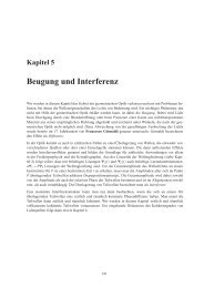
Section 4.1 APPLIED SUPERCONDUCTIVITY 1594.1 The dc-SQUID4.1.1 The Zero Voltage StateTwo superconducting Josephson junctions can be combined in parallel as shown in Fig. 4.1 to obtain asuperconducting quantum interference device known as the direct current superconducting quantuminterference device. The two superconducting junctions, which we will consider as lumped elements,are connected in parallel and joined by a superconducting loop. The two junctions are assumed to haveidentical critical current I c so that they are characterized by the current-phase relations I s1 = I c sinϕ 1 andI s2 = I c sinϕ 2 . Applying Kirchhoff’s law we obtain for the total current 7I s = I s1 + I s2 = I c sinϕ 1 + I c sinϕ( ) ( 2)ϕ1 − ϕ 2 ϕ1 + ϕ 2= 2I c cossin22. (4.1.1)The gauge-invariant phase differences ϕ 1 and ϕ 2 can be found by considering the line integral along thecontour shown in Fig. 4.1. We have to demand that the total phase change along the closed contour is2πn. Hence, in the same way as for the situation discussed in section 2.2.1 we obtain∮C∇θ · dl = 2π n= (θ Qb − θ Qa ) + (θ Pc − θ Qb ) + (θ Pd − θ Pc ) + (θ Qa − θ Pd ) + 2π n (4.1.2)Using ∇θ = 2πΦ 0(ΛJ s + A) (compare (2.2.2)) and ϕ = θ 2 − θ 1 − 2πΦ 0in analogy to section 2.2.1:θ Qb − θ Qa = +ϕ 1 + 2π ∫Q bΦ 0θ Pd − θ Pc = −ϕ 2 + 2πθ Pc − θ Qb =θ Qa − θ Pd =∫ P cQ b∫Q aP dΦ 02∫A · dl (compare (2.2.3)) we obtain1Q aA · dl (4.1.3)∫P dP cA · dl (4.1.4)∫P c∫P c∇θ · dl = + 2π ΛJ s · dl + 2π A · dl (4.1.5)Φ 0Φ 0Q b Q b∇θ · dl = + 2πSubstitution of (4.1.3) – (4.1.6) into (4.1.2) yieldsϕ 1 − ϕ 2 = − 2πΦ 0∮CA · dl − 2πΦ 0∫Q aΛJ s · dl + 2π ∫Q aΦ 0 Φ 0∫P cP dΛJ s · dl − 2π ∫Q aΦ 0Q bP dA · dl . (4.1.6)P dΛJ s · dl . (4.1.7)) ( )7 We use sinα + sinβ = 2sin( α+β2 cos α−β2 .2005

160 R. GROSS AND A. MARX Chapter 4II 1 I 2Q aI s1 =I s2 =I c sin ϕ 1I c sin ϕ 2Q bBP dP cFigure 4.1: The dc-SQUID formed by two Josephson junctions intersecting a superconducting loop. Theupper and the lower part of the loop can be represented by the macroscopic wave functions Ψ 2 = Ψ 20 exp(ıθ 2 )and Ψ 1 = Ψ 10 exp(ıθ 1 ), respectively. The broken line indicates the closed contour path of the integration.The integration of A is around a closed contour and therefore is equal to the total flux Φ enclosed by thesuperconducting loop. The integration of J s follows the same contour C but excludes the integration overthe insulating barrier. Furthermore, if the superconducting loop consists of a superconducting materialwith a thickness large compared to the London penetration depth λ L , the integration path can be takendeep inside the superconducting material where the current density is negligible. Therefore, the twointegrals involving the current density can be omitted and we obtainϕ 2 − ϕ 1 = 2πΦΦ 0. (4.1.8)We see that the two phase differences across the junctions are not independent but are linked to eachother via the boundary condition that we have to satisfy fluxoid quantization in the superconductingloop. Using expression (4.1.8) we can rewrite (4.1.1) as 8I s = 2I c cos(π Φ )sin(ϕ 1 + π Φ )Φ 0 Φ 0. (4.1.9)If the flux Φ threading the loop would be given just by the flux Φ ext due to the externally applied magneticfield, we would have solved the problem. Then, the maximum supercurrent of the parallel combinationis just given by∣ ( ∣∣∣Is m = 2I c cos π Φ )∣ext ∣∣∣. (4.1.10)Φ 08 Here, we use (ϕ 1 + ϕ 2 )/2 = [2ϕ 1 + (ϕ 2 − ϕ 1 )]/2 = ϕ 1 + (ϕ 2 − ϕ 1 )/2.© Walther-Meißner-Institut

Section 4.1 APPLIED SUPERCONDUCTIVITY 161However, in many cases we have to take into account the finite inductance L of the superconducting loop.Then, the flux Φ threading the loop is given by the sumΦ = Φ ext + Φ L (4.1.11)due to the applied magnetic field and the currents flowing in the loop. If we assume that the two sides ofthe loop are identical, we can write the currents flowing in the two arms of the loop aswhereI s1 = Ĩ + I cir (4.1.12)I s2 = Ĩ − I cir , (4.1.13)Ĩ = I s1 + I s22andI cir = I s1 − I s22(4.1.14)are the average current common in both arms and the current circulating in the loop, respectively. Notethat only the latter generates a net magnetic flux in the loop with the total flux then given byΦ = Φ ext + LI cir = Φ ext + LI c2 (sinϕ 1 − sinϕ 2 )( ) ( )ϕ1 − ϕ 2 ϕ1 + ϕ 2= Φ ext + LI c sincos22. (4.1.15)Using (4.1.8), we can write the total flux threading the loop as a function of Φ ext and ϕ 1 : 9Φ = Φ ext − LI c sin(π Φ )cos(ϕ 1 + π Φ )Φ 0 Φ 0. (4.1.16)We see that we have now two equations, (4.1.9) and (4.1.16), which determine the behavior of the dc-SQUID. These two equations have to be solved self-consistently. The maximum current Ism that canbe sent through the SQUID at a given Φ ext has to be found by maximizing (4.1.9) with respect to ϕ 1 ,however, with the constraint given by (4.1.16). This problem has been solved first by R. de BruynOuboter and A.Th.A.M. de Waele. 10In order to analyze limiting cases we introduce the so-called screening parameter β L defined asβ L ≡ 2LI cΦ 0. (4.1.17)This parameter represents the ratio of the magnetic flux generated by the maximum possible circulatingcurrent I cir = I c and Φ 0 /2. We also see that for β L = 1 the coupling energy 2E J = 2¯hI c /2e = Φ 0 I c /π ofthe two Josephson junctions is, apart from a factor 4/π, equal to the magnetic energy Φ 2 0 /8L due to themagnetic flux Φ 0 /2 stored in the superconducting loop.9 Here, we use sin(−α) = −sinα.10 R. de Bruyn Ouboter, A.Th.A.M. de Waele, Superconducting Point Contacts Weakly Connecting Two Superconductors,Progress in Low Temp. Phys. VI, C.J. Gorter ed., Elsevier Science Publishers (1970).2005

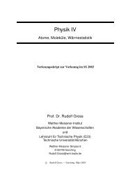
162 R. GROSS AND A. MARX Chapter 4I m s / I c(a)2.01.61.20.80.40.0-3 -2 -1 0 1 2 3Φ / Φ 03210-1-2-3-3 -2 -1 0 1 2 3Φ ext/ Φ 0 (b)Φ ext/ Φ 0Figure 4.2: (a) The maximum supercurrent Ism plotted versus the applied magnetic flux Φ ext for a dc-SQUIDwith two identical Josephson junctions in the limit β L ≪ 1. In (b) the flux threading the SQUID loop is plottedversus the applied flux Φ ext .Negligible Screening: β L ≪ 1In the case β L ≪ 1 the flux generated by the circulating current is small compared to the flux quantumand therefore can be neglected compared to Φ ext . At a given Φ ext the maximum supercurrent of thedc-SQUID is found by maximizing (4.1.9) with respect to ϕ 1 . From the condition dI s /dϕ 1 = 0 we obtain(cos ϕ 1 + π Φ )extΦ 0= 0 . (4.1.18)( )Thus, at the maximum we have sin ϕ 1 + π Φ extΦ 0= ±1 and the maximum value of the supercurrent isfound by taking the sign of the sine term. That is, we obtain the result∣ ( ∣∣∣Is m ≃ 2I c cos π Φ )∣ext ∣∣∣, (4.1.19)Φ 0which is of course equivalent to (4.1.10). As shown in Fig. 4.2, Ism is a periodic function of the externalflux. Note that for a loop area of 2 mm 2 an applied field of 1 nT results in Φ ext = Φ 0 , that is, theperiodicity of the curve corresponds to the very small field of 1 nT, which is more than four orders ofmagnitude smaller than the earth magnetic field.Large Screening: β L ≫ 1For large inductance L we have LI c ≫ Φ 0 and the circulating current tends to compensate the applied flux.The loop of the SQUID looks more and more like the single loop formed by a superconducting wire. Thissituation was discussed already in section 1.2 when we discussed flux quantization in multiply connectedsuperconductors. Consequently, the total flux in the loop will tend to be quantized:Φ = Φ ext + LI cir ≃ nΦ 0 . (4.1.20)Let us consider the case of large screening a bit more closely. The transport supercurrent through theSQUID is the sum of the currents passing junction 1 and 2:I s = I c sinϕ 1 + I c sinϕ 2 . (4.1.21)© Walther-Meißner-Institut

Section 4.1 APPLIED SUPERCONDUCTIVITY 16343Φ / Φ 0210-1β L = 2/πβ L = 1β L = 0.2-2-3-4β L = 2β L = 6-4 -3 -2 -1 0 1 2 3 4Φ ext/ Φ 0Figure 4.3: The total magnetic flux Φ plotted versus the applied magnetic flux Φ ext for a dc-SQUID with twoidentical Josephson junctions for different values of the screening parameter β L .On the other hand, the circulating screening current is given byI cir = I c2 (sinϕ 1 − sinϕ 2 ) . (4.1.22)Both (4.1.21) and (4.1.22) are constraint by the conditionϕ 2 − ϕ 1 = 2πΦΦ 0. (4.1.23)Note that here the magnetic flux is the sum of the external flux Φ ext and the flux Φ cir = LI cir due to thescreening current. Given the applied current I and the total flux Φ we have two equations for the twophase differences ϕ 1,2 and hence can solve for them and finally for Φ cir and Φ ext . For example, if I ≃ 0,we have sinϕ 1 ≃ −sinϕ 2 and obtainΦ ext = Φ + LI c sin(π Φ )Φ 0Φ ext= Φ + β (LΦ 0 Φ 0 2 sin π Φ )Φ 0or. (4.1.24)This relationship of course can be inverted to obtain Φ as a function of Φ ext as shown in Fig. 4.3.An interesting case occurs for Φ = nΦ 0 , for which ϕ 1 = ϕ 2 + n2π, so that I cir = 0 and Φ = Φ ext . We seethat the SQUID response to Φ ext in integer multiples of Φ 0 is not affected by the screening. However,for practical applications it is often required that the relation between Φ and Φ ext is single-valued andnon-hysteretic. As shown by Fig. 4.3 this is possible only for small values of the screening parameterβ L . This results from the fact that the maximum possible value of Φ cir is LI c . Since roughly speakinga multivalued relationship between Φ and Φ ext can be avoided only for |Φ cir | ≤ Φ 0 /2, we immediatelysee that this is equivalent to LI c ≤ Φ 0 /2 or β L = 2LI c /Φ 0 ≤ 1. A more detailed analysis shows that ahysteretic Φ(Φ ext ) dependence can be avoided for β L ≤ 2/π.2005

164 R. GROSS AND A. MARX Chapter 4We still have to discuss the dependence of the supercurrent on the applied magnetic flux. From (4.1.20)we obtain for large β LI cir ≃ − Φ ext − nΦ 0L. (4.1.25)We see that I cir → 0 for large L. Then, the applied current divides about equally in the two SQUIDarms. The maximum current is obtained to Ism ≃ 2I c . When n is initially zero, a small screening currentI cir ≃ −Φ ext /L will flow to screen the applied magnetic field. Therefore, the current I 1 will tend todecrease and I 2 to increase with increasing Φ ext . However, since I 2 ≤ I c , it will be fixed at I c as I 1decreases asI 1 ≃ I c − 2Φ extL. (4.1.26)With this expression for I 1 and I 2 ≃ const ≃ I c we obtainIs m ≃ 2I c − 2Φ extor (4.1.27)LIsm ≃ 1 − 2Φ ext 1. (4.1.28)2I c Φ 0 β LWe see that the modulation of the maximum supercurrent of the SQUID by the applied magnetic flux isstrongly decreasing with increasing β L roughly proportional to 1/β L .4.1.2 The Voltage StatePractical dc-SQUIDs are not operated in the zero voltage state. They are operated at a constant biascurrent above the maximum supercurrent I m s (0) at zero applied magnetic flux. That is, the SQUID is inthe voltage state. We will show that in this situation the dc-SQUID produces an output voltage that isrelated to the applied magnetic flux.Negligible screening: β L ≪ 1, strong damping: β C ≪ 1In order to discuss the dependence of the SQUID voltage on the applied magnetic flux we start with thelimit of negligible screening. In this case the total flux in the SQUID loop is just given by the appliedflux. We further assume that the junction capacitance is negligible small, that is, we consider the case ofstrongly overdamped Josephson junctions (β C ≪ 1) and that the two junctions are identical. Then, weonly have to consider the Josephson current and the resistive current givingI = I c sinϕ 1 + I c sinϕ 2 + V + V R N R N= 2I c cos(π Φ )sin(ϕ 1 + π Φ )+ 2 V . (4.1.29)Φ 0 Φ 0 R NHere, we have used (4.1.1) and (4.1.8). Let us define the new phaseϕ = ϕ 1 + π Φ Φ 0(4.1.30)© Walther-Meißner-Institut

Section 4.1 APPLIED SUPERCONDUCTIVITY 165Figure 4.4: Current-voltage characteristics of a dc-SQUID in the limit β L ≪ 1, β C ≪ 1 for different values ofthe applied magnetic flux Φ ext for a dc-SQUID with two identical Josephson junctions.and note that due Φ ≃ Φ ext = const we havedϕdt= dϕ 1dt= 2πΦ 0V (t) . (4.1.31)Then, we can rewrite (4.1.29) asI = I m s (Φ ext ) sinϕ + 2R N2π dϕΦ 0 dt(4.1.32)with(Is m (Φ ext ) = 2I c cos π Φ )extΦ 0. (4.1.33)We see, that equation (4.1.32) represents the equation of a single Josephson junction with a maximumJosephson current that depends on the external flux. For a single junction we have used the pendulumas a mechanical analog. In the same way we can use two pendula that are coupled to each other as theanalogue for the dc-SQUID. In the case of negligible screening (β L ≪ 1) the coupling of the two pendulais rigid as can be seen from (4.1.30) and they move with the same angular velocity according to (4.1.31).Note that the rigid coupling is no longer true for significant screening (β L ≥ 1).Due to the equivalence of the dc-SQUID with a single junction having a flux dependent maximumJosephson current, the current-voltage characteristic of the dc-SQUID is just given by the RSJ-model2005

166 R. GROSS AND A. MARX Chapter 4result (3.3.8):〈V (t)〉 = I c R N√ ( I2I c) 2−( I m s (Φ ext2I c)√2 ( ) I 2 [ (= I c R N − cos π Φ )] 2ext. (4.1.34)2I c Φ 0The IVCs obtained according to this equation are shown in Fig. 4.4. It can be seen that the IVCs areperiodic with the applied magnetic flux with the periodicity of a single flux quantum. Considering thetime-averaged junction voltage as a function of the applied flux for different values of the bias current wesee that these curves are also periodic with the same periodicity. Furthermore, the minima and maxima ofthe 〈V 〉(Φ ext ) always appear at the same flux values. Fig. 4.4 also shows the cosπΦ ext /Φ 0 dependence ofthe zero voltage supercurrent through the SQUID. Furthermore, it is seen that the maximum modulationof the time-averaged voltage with varying applied flux occurs for I ≃ 2I c .Finite screening: β L ∼ 1, intermediate damping: β C ∼ 1For practical SQUIDs the inductance L of the loop containing the Josephson junctions must be takeninto account. As already discussed above, the loop area should be made large in order to increase theflux threading the SQUID at a given field value. However, a large loop area can not be obtained withoutincreasing the loop inductance. Furthermore, for typical Josephson junctions we cannot neglect thedisplacement current due to the finite junction capacitance as well as the fluctuating noise current. In thisgeneral case the dc-SQUID circuit is governed by a set of time-dependent nonlinear equations that mustbe solved numerically.The phase differences across the two junctions have to satisfy the following equations: 11,12,13V = Φ 04π( dϕ1dt+ dϕ )2dt2πn = ϕ 2 − ϕ 1 − 2π Φ extI2I2(4.1.35)− 2π LI cirΦ 0 Φ 0(4.1.36)= ¯hC d 2 ϕ 12e dt 2 + ¯h dϕ 1+ [I c sinϕ 1 + I cir ] + I F12eR N dt(4.1.37)= ¯hC2ed 2 ϕ 2dt 2 + ¯h dϕ 2+ [I c sinϕ 2 − I cir ] + I F2 . (4.1.38)2eR N dtEquation (4.1.35) relates the SQUID voltage to the rate of phase change. Note that for negligible screeningwe have dϕ 1dt= dϕ 2dtand the usual voltage-phase relation is recovered. For finite screening this isno longer the case and we have dϕ 1dt≠ dϕ 2dt. Equation (4.1.36) expresses the fluxoid quantization in thesuperconducting loop. We see that in contrast to negligible screening (compare (4.1.8)) we have to takeinto account also the flux LI cir due to the finite inductance of the loop. Equations (4.1.37) and (4.1.38)are Langevin equations coupled via I cir . These coupled equations have to be solved numerically underthe constraint given by (4.1.36) as a function of the screening parameter β L = 2LI c /Φ 0 , the Stewart-McCumber parameter β C = 2πI c R 2 N C/Φ 0 and the thermal noise parameter γ = 2πk B T /I c Φ 0 .11 C.D. Tesche, J. Clarke, dc-SQUID: Noise and Optimization, J. Low Temp. Phys. 27, 301 (1977).12 J.J.P. Bruines, V.J. de Waal, J.E. Mooij, J. Low Temp. Phys. 46, 383 (1982).13 V.J. de Waal, P. Schrijner, R. Llurba, Simulation and Optimization of a dc-SQUID with Finite Capacitance, J. Low Temp.Phys. 54, 215 (1984).© Walther-Meißner-Institut

Section 4.1 APPLIED SUPERCONDUCTIVITY 167(a)(b)ϕ 1ll´ϕ 2lΜ2ΜI c sin ϕ 1ΜI c sin ϕ 2ϕ 1 −ϕ 2ϕ 2lϕ 1lI c sin ϕ 2l´2ΜΜ½ (ϕ 1 +ϕ 2 )I c sin ϕ 1ΜFigure 4.5: The pendulum analogue of a dc SQUID. The pendula are rigidly attached to the bar and thebar can rotate. At negligible screening (β L ≪ 1) the bar connecting the two pendula is rigid resulting in acombined pendulum with mass 2M at the center of mass. (a) Zero applied bias current and (b) finite biascurrent. The combined pendulum is shown in the center using grey lines.Mechanical AnalogueWe can gain insight into the equations of motion of a dc-SQUID by the pendulum analogue (see Fig. 4.5)already used for the single Josephson junction. The dc-SQUID formed by two identical junctions can bemodeled by two pendula with the same mass M and length l hanging from the same pivot point with thetwo pendula coupled via a twistable bar. The case of negligible screening (β L = 0) corresponds to thecase that the connecting bar is rigid. The relative angle ϕ 1 − ϕ 2 = 2πΦ ext /Φ 0 is fixed by the externalflux. That is, in effect we have to deal with a single combined pendulum with its full mass 2M located atthe center of mass halfway between the two individual masses, which is at distance l ′ = lcos[ 1 2 (ϕ 1 −ϕ 2 )]from the pivot point. Alternatively, we can consider the net gravitational torque (corresponding to the netcritical current) as the vector sum of those of the two pendula. In the absence of an applied torque (appliedcurrent) the combined pendulum hangs with the center of mass pointing down with the individual pendulaat 1 2 (ϕ 1 − ϕ 2 ) on either side (see Fig. 4.5a). Note that for (ϕ 1 − ϕ 2 ) = π corresponding to Φ ext = Φ 0 /2the center of mass is at the pivot point. As a torque (bias current) is applied this is rotating the combinedpendulum (see Fig. 4.5b). The circulating current I cir = 1 2 (I c sinϕ 1 − sinϕ 2 ) is half the difference of thehorizontal projections of the two pendula.In the case of finite screening (β L > 0) the situation is a little bit more complicated, since now the barconnecting the two pendula is no longer rigid but flexible. We can regard it as a torsional spring on therotation axis with a loose spring corresponding to a large loop inductance and hence a large screeningeffect. An applied flux again results in a finite angle ϕ 1 − ϕ 2 = 2πΦ/Φ 0 , which is given now by thetotal flux Φ = Φ ext + LI cir . For a large inductance L the applied flux is well screened by the circulatingcurrent so that Φ ∼ 0. That means, that also ϕ 1 − ϕ 2 ∼ 0 at zero bias current. This is evident from ourmechanical analogue. A large inductance corresponds to a loose spring connecting the pendula. Hence,the applied flux tries to rotate the pendula in opposite directions but they will stay in their bottom positionand twist the loose spring connecting them. Due to the loose spring the difference ϕ 1 − ϕ 2 is no longerconstant as in the case of negligible screening and hence dϕ 1dt≠ dϕ 2dt. As the inductance becomes smallerthe connecting spring becomes stiffer and finally rigid at β L → 0.2005

168 R. GROSS AND A. MARX Chapter 44.1.3 Operation and Performance of dc-SQUIDsThe principle of operation of a dc-SQUID is shown in Fig. 4.6. The two junctions, which are modeledby the RCSJ model, are connected in parallel in a superconducting loop with inductance L. In orderto eliminate hysteretic IVCs, the Stewart-McCumber parameter of the junctions is restricted to β C ≤ 1.In practice, this is usually achieved by using external shunt resistors (see Fig. 4.11). The IVCs of theSQUID depend on the applied magnetic flux as shown in Fig. 4.4 for β C ≪ 1 and β L ≪ 1. In Fig. 4.6bonly the IVCs with the largest (Φ ext = nΦ 0 ) and the smallest critical current (Φ ext = (n + 1 2 )Φ 0) areshown. When the SQUID is biased at a constant current I > 2I c , the time-averaged voltage 〈V 〉 of theSQUID varies periodically with the applied flux with period Φ 0 as shown in Fig. 4.6c.For practical applications the flux threading the loop has to be measured with high resolution. Therefore,the SQUID is operated at the steepest part of the 〈V 〉(Φ ext ) curve, where the flux-to-voltage transfercoefficientH≡( ∂V∣∂Φ ext)I=const∣ (4.1.39)is a maximum. We see that the dc-SQUID can be considered as a flux-to-voltage transducer, whichproduces an output voltage in response to small variations of the input flux.The resolution of the SQUID can be characterized by the equivalent flux noise Φ F (t), which has thepower spectral densityS Φ ( f ) = S V ( f )H 2 (4.1.40)at a given frequency f . Here, S V ( f ) is the power spectral density of the voltage noise across the SQUIDat a fixed bias current. The flux noise power spectral density is inconvenient for comparing the noise inSQUIDs with different values of the loop inductance. A more convenient characterization of the noise isto use the noise energy ε( f ) associated with S Φ ( f ):ε( f ) = S Φ( f )2L= S V ( f )2LH 2 . (4.1.41)The noise energy of the dc-SQUID sets the energy resolution of the SQUID, which for practical applicationsshould be as small as possible. For a given S V ( f ) we therefore have to maximize H and L. Using aplausibility consideration we see the following:1. Bias current I: In order to maximize H we should choose a bias current just above 2I c , since herethe modulation of the 〈V 〉(Φ ext ) curve is largest.2. Flux bias: For optimum bias current the flux bias should be close to (2n + 1)Φ 0 /4, since here His maximum.© Walther-Meißner-Institut

Section 4.1 APPLIED SUPERCONDUCTIVITY 169II FR NCI cΦI cCR NI FV(a)L2.02.01.6Φ ext = (n+ ½) Φ 01.6 / I cR N1.20.8 / I cR N1.20.80.4Φ ext = n Φ 00.4(b)0.00.0 0.5 1.0 1.5 2.00.00 1 2 3I / 2I c (c)Φ ext/ Φ 0Figure 4.6: (a) The equivalent circuit of a dc-SQUID, (b) the current-voltage characteristics for two differentvalues of the applied magnetic flux (Φ ext = nΦ 0 and Φ ext = (n + 1/2)Φ 0 ) and (c) the time-averaged voltageplotted versus the applied flux for different values of the bias current (I/2I c = 1.001, 1.01, 1.1, 1.2. 1.4, 1.6,1.8, and 2.0).3. Junction critical current I c : The junction critical currents should be much larger than the thermalnoise current, or equivalently, the coupling energy I c Φ 0 /2π should be much larger the the thermalenergy k B T . In this way, noise rounding of the IVCs as shown in Fig. 3.18 is avoided, which woulddeteriorate H. Computer simulations show that 1415 · I c I th ≡ 2πk BT(4.1.42)Φ 0is sufficient. At 4.2 K this condition, which is equivalent to asking for a sufficient coupling ofthe phases of the superconducting wave functions across the two Josephson junctions, implies thatI c 1 µA.4. The loop inductance L: The loop inductance should be as large as possible for optimum sensitivity.However, at a given temperature T the thermal energy k B T causes a root mean squarethermal noise flux in the loop, 〈Φ 2 th 〉1/2 = √ k B T L. This noise flux should be considerably smallerthan Φ 0 giving an upper bound for L. We can define a thermal inductance L th as the inductancevalue, for which the thermal noise current I th generates just half a flux quantum in the loop, that isL th I th = Φ 0 /2 or 2L th I th /Φ 0 = 1. In order to keep the effect of thermal fluctuations small, the loopinductance L of the SQUID has to be sufficiently smaller than L th . Again, computer simulations14 J. Clarke, R. Koch, The Impact of High Temperature Superconductivity on SQUIDs, Science 242, 217 (1988).2005

170 R. GROSS AND A. MARX Chapter 4show that5 · L L th ≡ Φ 02I th= Φ2 04πk B T(4.1.43)is sufficient. This constraint, which is equivalent to asking for a sufficient coupling of the phasedifferences of the two junctions, implies that L 1 nH at 4.2 K.In analogy to the screening parameter β L we can define the parameterβ th = 2I thLΦ 0= LL th= I thI cβ L = γ β L (4.1.44)with γ = I th /I c (compare (3.1.17)). This parameter is of crucial importance for the SQUID performance(see Fig. 4.7).5. The screening parameter β L : The screening parameter β L = 2I c L/Φ 0 has to be smaller thanunity to avoid hysteretic 〈V 〉(Φ ext ) curves. This condition can be easily satisfied by making Lsmall. However, we already have seen that we should make L as large as possible to increase theSQUID sensitivity. Therefore, we should choose β L ≃ 1, i.e. as large as possible. For β L ≃ 1and taking the smallest possible I c value at 4.2 K (∼ 1 µA), we obtain L 1 nH, which is stillcompatible with the constraint given by (4.1.43). 156. The Stewart-McCumber parameter β C : The Stewart-McCumber parameter has to be smallerthan unity in order to avoid hysteretic IVCs. For superconducting tunnel junctions, which intrinsicallyhave large capacitance and hence β C ≫ 1, this is achieved by using an external shunt resistorsmaller than the normal resistance of the junction (see Fig. 4.11). That is, in principle it is not aproblem to satisfy the condition β C ≤ 1. However, using a small shunt resistor R shunt ≪ R N reducesthe voltage amplitude of the 〈V 〉(Φ ext ) curves to I c R shunt ≪ I c R N . Therefore, R shunt should be aslarge as possible, that is, we have to choose β C ≃ 1.The detailed values of the parameters describing the performance of the SQUID have to be evaluatedby numerical simulations. 16,17,18,19 These simulations show that the noise energy of dc-SQUIDs has aminimum for β L ≃ 1, β C ≃ 1, for a flux bias close to (2n + 1)Φ 0 /4 and for a bias current I, for which thevoltage modulation of the 〈V 〉(Φ ext ) curves is largest. Since the maximum voltage modulation is aboutI c R N we haveH ≃ I cR NΦ 0 /2 ≃ R NL(4.1.45)for β L ≃ 1. In the white noise regime 20 the voltage noise of the SQUID can be estimated by splitting upthe current noise power spectral density S I into an in-phase part SIin = 4k B T /(R N /2) and an out-of-phase15 Note that for high temperature superconductor dc-SQUIDs the operation temperature is about 20 times higher and thereforewe have the constraint I c 20 µA and L 50 pH. Again, for β L ≃ 1 we obtain with I c ≃ 20 µA an inductance value L 50 pH,which is compatible with the thermal constraint. However, due to the smaller inductance value it is in general more difficult tocouple magnetic flux into the SQUID loop.16 C.D. Tesche, J. Clarke, dc-SQUID: Noise and Optimization, J. Low Temp. Phys. 27, 301 (1977).17 D. Drung, W. Jutzi, IEEE Trans. Magn. 21, 330 (1985).18 D. Kölle, R. Kleiner, F. Ludwig, E. Dantsker, J. Clarke, High-transition-temperature superconducting quantum interferencedevices, Rev. Mod. Phys. 71, 631 (1999).19 J. Clarke, A.I. Braginski (eds.), The SQUID Handbook, Vol. 1: “Fundamentals and Technology of SQUIDS and SQUIDSystems” Wiley-VCH, Weinheim (2004).20 The low-frequency regime, where 1/ f noise dominates is not discussed here.© Walther-Meißner-Institut

Section 4.1 APPLIED SUPERCONDUCTIVITY 171part SIout = 4k B T /2R N . Note that for the in-phase current fluctuations, which have the same direction inthe two arms of the SQUID, the relevant resistance is R N /2 due two the parallel connection of the twojunction resistors. In contrast, for the out-of-phase part, which is in opposite direction in the two armsand results in a circulating current, the relevant resistance is 2R N due to the series connection of the twojunctions resistors for the circulating current. In a small signal analysis the voltage noise power spectraldensity due to the in- and out-of-phase current fluctuations is given by 21,22,23S V ( f ) = SI in ( f )R 2 d + SIout ( f ) L 2 H 2 = 4k [BT2R 2 d + L2 H 2 ]R N 2, (4.1.46)where R d is the differential resistance at the operation point. With the optimum values H ∼ R N /L andR d ∼ √ 2R N obtained from numerical simulations we obtainS V ( f ) ≃ 4k [ ]BT4R 2 N + R2 NR N 2The noise energy then can be estimated to= 18k B T R N . (4.1.47)ε( f ) = S V ( f )2LH 2≃ 9k BT LR N≃ 9k BT Φ 02I c R Nfor β L ≃ 1 . (4.1.48)We see that the noise energy increases with temperature and decreasing I c R N product of the Josephsonjunctions. If we eliminate R N by using β C = 2πI c R 2 N C/Φ 0 ≃ 1 and if we also eliminate L by usingβ L = 2I c L/Φ 0 ≃ 1 we obtainε( f ) ≃ 16k B T≃√LCβ C16 √ √Φ0 C sπk B T2πJ c= 16√ πk B Tω pfor β L ≃ 1; β C ≃ 1 . (4.1.49)Here, C s = C/A is the specific junction capacitance and J c = I c /A the critical current density of thejunction. We see that we can improve the performance of the dc-SQUID by reducing the temperatureas well as by decreasing the capacitance and by increasing the critical current density, i.e. by increasingthe plasma frequency of the Josephson junctions. Today critical current densities above 10 3 A/cm 2 areused requiring junction areas of the order of 1 µm 2 for realizing critical current values of a few µA.Until today, a large number of dc-SQUIDs has been studied and it was found that their performanceagrees well with the predictions of the numerical simulations. Today it is common to quote the noise21 We note that in a more detailed analysis the voltage noise of a single Josephson junction at a measuring frequency f muchsmaller than the Josephson frequency f J is given byS V ( f ) = 4k BTR NR 2 d + 4k BTR NR 2 d( )1 2 Ic,2 Iwhere the first term is the usual Nyquist noise and the second represents the Nyquist noise generated at frequencies f J ± f mixeddown to the measurement frequency by the Josephson oscillations due to the nonlinearity of the IVC. The factor 1 2( IcI) 2is themixing coefficient, which vanishes at large bias currents I ≫ I c . Furthermore, at sufficiently high bias currents the Josephsonfrequency exceeds k B T /h and quantum corrections become important (compare section 3.5.5).22 K.K. Likharev, V.K. Semonov, JETP Lett. 15, 442 (1972).23 R.H. Koch, D.J. van Harlingen, J. Clarke, Phys. Rev. Lett. 45, 2132 (1980).2005

172 R. GROSS AND A. MARX Chapter 4Σ / Σ(γβ L=1/80)10Σ (γβ L=1/80)64200 2 4 6β Lβ L0.60.70.81.01.52.03.04.010.01 0.1 1Figure 4.7: Calculated reduced energy resolution Σ(γβ L ) normalized to Σ(γβ L = 1/80). Inset shows Σ(γβ L =1/80) versus β L (data from D. Kölle et al., Rev. Mod. Phys. 71, 631 (1999)).γβ Lenergy of SQUIDs in units of ¯h ≃ 10 −34 Js. Optimized SQUIDs have a noise energy approaching thequantum limit ¯h. However, these SQUIDs have very low inductance and therefore are not useful for mostapplications requiring optimum magnetic field resolution. Best practical dc SQUIDs have reached anenergy resolution of some 10¯h. 24A recent result of a numerical simulation is shown in Fig. 4.7. Here, the reduced noise energyΣ( f ) = ε( f )2Φ 0 k B TI c R N(4.1.50)is plotted versus the dimensionless parameterβ th = γβ L = 2πk BTI c Φ 02I c LΦ 0= L Φ 2 04πk B T≡LL th. (4.1.51)For γβ L ≤ 0.2 corresponding to L ≤ 1 5 L th, the reduced noise energy is almost constant, while for highervalues of γβ L it increases rapidly. The rapid increase in noise energy arises from the rapid degradationof the transfer function with increasing γβ L = L/L th due to thermal noise rounding of the IVCs.4.1.4 Practical dc-SQUIDsPractical dc-SQUIDs do not only consist of the SQUID loop discussed so far, but also of an antenna anda room temperature electronics as schematically shown in Fig. 4.8. The antenna has both to transfer thequantity that has to be measured into magnetic flux and to couple this flux effectively into the SQUIDloop. The SQUID itself acts as a flux-to-voltage transducer. The room temperature electronics has toamplify the voltage signal as well as to provide the current and flux bias.24 A.A. Jin, T.R. Stevenson, F.C. Wellstood, W.W. Johnson, IEEE Trans. Appl. Supercond. AS-7, 2742 (1997).© Walther-Meißner-Institut

Section 4.1 APPLIED SUPERCONDUCTIVITY 173I cΦI cVantenna:signal-to-fluxconverterSQUID:flux-to-voltagetransducerelectronics:voltage amplification,bias signalsFigure 4.8: The practical dc-SQUID consisting of an antenna acting as a signal-to-flux converter, the SQUIDloop acting as the flux-to-voltage transducer, and the room temperature electronics.The Washer Type dc-SQUIDObviously, a large area A of the SQUID loop is advantageous to increase the sensitivity of a SQUID,since small field changes ∆B then result in large flux changes ∆Φ ext = A · ∆B. However, a large A alsoresults in a large loop inductance L, which may deteriorate the SQUID performance as discussed above.Based on this conflicting requirements various SQUID designs have been developed. In the 1970ies and1980ies, often three-dimensional loop geometries have been used for the realization of SQUIDs (e.g. byevaporation of a cylinder containing the Josephson junctions on a thin quartz thread).Today dc-SQUIDs are based on thin film structures, which are patterned using optical and electron beamlithography. Here, a large effective loop area at small loop inductance can be achieved by making use ofthe perfect diamagnetism of superconductors. As shown in Fig. 4.9, instead of a narrow superconductingloop structure a broad “washer-type” structure can be used. Such geometries have been successfullyused for high T c dc-SQUIDs using grain boundary Josephson junctions. 25,26,27 The washer design wasfirst proposed by M.B. Ketchen and therefore these SQUID structures today are denoted as KetchentypeSQUIDs. 28 This geometry also helps to overcome the problem of coupling the magnetic flux of theantenna system effectively to the SQUID loop of a thin film SQUID. In 1981 M.B. Ketchen and J.M.Jaycox introduced the idea of depositing a planar spiral input coil on a dc-SQUID in a square washergeometry. 29,30 The thin film planar coil is separated from the SQUID washer only by a thin insulatinglayer. A typical washer type dc-SQUID is shown schematically in Fig. 4.11. The square washer formsthe SQUID loop. It contains a narrow slit, which is closed by a superconducting line containing the twojunctions, which are located at the outer rim of the washer.For the washer geometry shown in in Figs. 4.9 and 4.11, the loop currents circulate around the inneropening (hole or slit) of the washer, which then determines the inductance of the SQUID loop. Jaycoxand Ketchen showed that a square washer with a hole of diameter D (without slit) and an outer edge W25 R. Gross et al., Appl. Phys. Lett. 57, 727 (1990).26 R. Gross et al., Physica C 170, 315 (1990).27 D. Kölle et al., Rev. Mod. Phys. 71, 631 (1999).28 M.B. Ketchen, IEEE Trans. Magn. MAG-17, 387 (1980).29 M.B. Ketchen, J.M. Jaycox, Ultra-low Noise Tunnel Junction dc-SQUID with a Tightly Coupled Planar Input Coil, Appl.Phys. Lett. 40, 736 (1982).30 J.M. Jaycox, M.B. Ketchen, Planar Coupling Scheme for Ultra-low Noise dc-SQUIDs, IEEE Trans. Magn. 17, 400 (1981).2005

174 R. GROSS AND A. MARX Chapter 4I I ID D DW W WFigure 4.9: Sketch of various geometries for planar dc-SQUIDs with washer geometry.has the inductanceL ≃ 1.25 µ 0 D (4.1.52)in the limit W ≫ D. That is, the loop inductance scales with the inner diameter D. In contrast, theeffective area of the SQUID loop is 31A eff ∝ D ·W , (4.1.53)that is, it scales with the outer dimension of the washer. Of course, one cannot increase W arbitrarily,since for large W one starts to trap magnetic flux quanta in the washer area during cool down even insmall magnetic fields. The thermally activated motion of these flux quanta generate disturbing 1/ f -noise.An experimental example for the flux focusing effect is shown in Fig. 4.10 for a geometry shown in theinset. Here, A eff /D 2 is plotted versus W 2 /D 2 on a double logarithmic scale. In such plot a straight linewith slope 1/2 is expected according to (4.1.53) in good agreement with the data.We briefly address the inductance and the coupling of a spiral input coil that can be put on top of thewasher as shown in Fig. 4.11. Neglecting the parasitic inductance associated with the Josephson junctions,the following expressions for the inductance L i of the spiral input coil, the mutual inductance M iand the coupling coefficient α 2 between the spiral and the SQUID loop are found:L i ≃ n 2 L + L s (4.1.54)M i ≃ √ n 2 L · L = nL (4.1.55)α 2 ≃11 + L s /n 2 L . (4.1.56)Here, L s is the stripline inductance of the spiral coil, n the number of turns of the spiral input coil andn 2 L the geometric self-inductance of the input coil. For the estimate of M i we have assumed that the fluxdue to a current flowing in the spiral input coil is perfectly coupled in the SQUID hole. The couplingcoefficient α is obtained from the expression α = M i / √ L i L = nL/ √ (n 2 L + L s )L. As an example, forD = 20 µm we obtain L ≃ 30 pH. For a 50 turn input coil we obtain L i ≃ 75 nH 32 and M i ≃ 1.5 nH. The31 M.B. Ketchen, W.J. Gallagher, A.W. Kleinsasser, S. Murphy, J.R. Clem, in SQUID’85, H.D. Hahlbohm and H. Lübbigeds., Walther de Gruyter, Berlin (1985), p. 865.32 The stripline inductance is usually negligible for a 50 turn coil.© Walther-Meißner-Institut

Section 4.1 APPLIED SUPERCONDUCTIVITY 175A eff/ D 210 1DW10 010 0 10 1 10 2W 2 / D 2Figure 4.10: Flux focusing effect in a washer-type YBa 2 Cu 3 O 7−δ grain boundary junction dc SQUID measuredat 77 K. The dashed line shows the theoretical dependence expected according to (4.1.53). The deviations atlarge W 2 /D 2 values are caused by the finite slit inductance of the used washer geometry shown in the inset(data according to R. Gross et al., Appl. Phys. Lett. 57, 727 (1990)).experimentally determined coupling coefficient typically ranges between 0.6 and 0.8. A specific problemof the washer-type dc SQUID geometry is the considerable capacitance between the spiral input coil andthe square washer. This can result in LC-resonances. These resonances, in turn, result in structuresin the IVCs, which can give rise to excess noise. The effect of the LC-resonances can be reduced byreducing the number of turns on the washer and thereby reducing the parasitic capacitance (in this casean intermediate superconducting transformer can be used to couple in the signal). On the other hand, theshunt resistance of the junctions can be decreased thereby increasing the damping.Low-T c dc-SQUIDs: Low-T c dc SQUIDs are fabricated using standard multilayer thin film technology(cf. Fig. 4.11). In order to increase the energy sensitivity, Josephson junctions with a high plasmafrequency have to be used. This is achieved by using high critical current density junctions, which allowto minimize the junction area and hence the junction capacitance. Although various materials combinationshave been used so far, the most successful is the combination of niobium and aluminium. Thiscombination is stable in time and not affected by thermal cycling. Furthermore, Nb/AlO x /Nb tunnel junctionsshow a low level of 1/ f noise due to critical current fluctuations compared to e.g. NbN/MgO/NbNjunctions.High-T c dc-SQUIDs: Today high-T c dc-SQUIDs are also fabricated using multilayer thin film technology.However, in contrast to low-T c materials an heteroepitaxial growth of the different superconductinglayers is required to avoid grain boundaries in the thin film structures. These are known to beresponsible for a high level of 1/ f -noise. A further problem in the fabrication of high-T c dc-SQUIDs isthe poor reproducibility of the junctions. Various junction types such as grain boundary junctions, rampjunctions or edge junctions have been used with different success. 33,34Due to the problem of heteroepitaxial growth of multilayer structures the integration of the input coil33 R. Gross, P. Chaudhari, Status of dc-SQUIDs in the High Temperature Superconductors, in Principles and Applications ofSuperconducting Quantum Interference Devices, pp. 419–479, A. Barone ed., World Scientific, Singapore (1992).34 For a more recent review see D. Kölle et al., Rev. Mod. Phys. 71, 631 (1999).2005

176 R. GROSS AND A. MARX Chapter 4washerspiralinputcoilSiO 2insulationlayerJosephsonjunctionsNb baseelectrodeSiO 2500 µmJosephsonjunctionsIPb topelectrodeshuntresistorFigure 4.11: Sketch of a Nb/Pb dc-SQUID using a square washer geometry and a planar spiral input coil. Thejunction area is shown on an enlarged scale on the right. Also shown is an optical micrograph of a washer-typePb/Nb dc-SQUID (by courtesy of J. Clarke).on a washer structure is still a challenge for high-T c SQUIDs. 35,36 Therefore, often so-called flip-chipstructures have been applied where the input coil is fabricated on a separate chip and then flip-chippedon the washer. 37In order to avoid complicated multilayer structures it is also common to use directly coupled high-T c dc-SQUIDs. Here, the SQUID loop is directly coupled to a parallel loop that acts as a signal pick-up loop.The big advantage of such directly coupled SQUIDs is the fact that only a single superconducting layer isrequired that can be grown with high quality on a single or bi-crystalline substrate. A schematic drawingof such a SQUID can be found in Fig. 4.22). For such directly coupled dc-SQUIDs field sensitivitiesdown to 20 fT/ √ Hz have been obtained in the white noise regime at 77 K. 384.1.5 Read-Out SchemesThe Flux-Locked Loop OperationThe 〈V 〉(Φ ext ) curves of the dc-SQUID are nonlinear. Therefore, a linear relation between an input signaland the output voltage is obtained only in the small signal limit. This problem can be solved by usingthe SQUID in a feedback circuit as a null-detector for magnetic flux. 39 One simply applies an oscillatingmagnetic flux with a peak-to-peak amplitude of about Φ 0 /2 and a frequency f mod in the 100 kHz regimeas shown in Fig. 4.12. If the quasistatic flux is exactly nΦ 0 , the resulting ac voltage is a rectified version35 J.W.M. Hilgenkamp, G.C.S. Brons, J.G. Soldevilla, R.P. Ijsselstein, J. Flokstra, H. Rogalla, Appl. Phys. Lett. 64, 3497-3499 (1994).36 B. David, D. Grundler, J.P. Krumme, O. Doessel, IEEE Trans. Appl. Supercond. AS-5, 2935-2938 (1995).37 P.A. Nilsson, Z.G. Ivanov, E.A. Stephantsov, H.K. Hemmes, J.W.M. Hilgenkamp, J. Flokstra, Inst. Phys. Conf. Ser. 148,1537-1540 (1995), D. Dew-Highes ed., Institute of Physics, Bristol.38 D. Kölle, A.H. Micklich, F. Ludwig, E. Dantsker, D.T. Nemeth, J. Clarke, Appl. Phys. Lett. 63, 2271-2273 (1993).39 J. Clarke, W.M. Goubau, M.B. Ketchen, J. Low. Temp. Phys. 25, 99 (1976).© Walther-Meißner-Institut

Section 4.1 APPLIED SUPERCONDUCTIVITY 177VVΦ(c)ΦΦ = n Φ 0V LΦΦ = (n+ 1/4) Φ 0(a)(n+1/2) Φ 0(b)Figure 4.12: Flux modulation scheme for a dc-SQUID showing the voltage across the SQUID for (a) Φ = nΦ 0and (b) Φ = (n + 1 4 )Φ 0. In (c) the output signal V L of the lock-in amplifier is plotted versus the applied flux.of the input signal. That is, it contains only a 2 f mod frequency component. If this signal is detected bya lock-in amplifier referenced to the fundamental frequency f mod , the resulting output voltage is zero.In contrast, if the quasistatic flux is (n + 1 4 )Φ 0, the voltage across the SQUID is at f mod and the outputsignal from the lock-in amplifier will be maximum. Thus, increasing the flux from nΦ 0 to (n + 1 4 )Φ 0 thelock-in output signal will increase, whereas it will increase in the negative direction on decreasing theflux from nΦ 0 to (n − 1 4 )Φ 0. Instead of a sinusoidal a square-wave flux signal can be used. Then, forthe operation point Φ = nΦ 0 and a peak-to-peak amplitude of Φ 0 /2 the SQUID is biased at the points ofmaximum slope of the 〈V 〉(Φ ext ) curve for each half-wave of the square-wave signal.The ac voltage across the SQUID is usually coupled to a low noise preamplifier via a cooled transformer,which results in an increase of the low SQUID impedance from R d to N 2 R d , where R d is the differentialresistance of the SQUID at the operation point and N the turns-ratio of the transformer. One also canuse a cooled LC series resonant circuit, which provides an impedance Q 2 R d , where Q is the quality ofthe tank circuit. The values of N or Q are chosen to obtain an optimum impedance match between theSQUID and the room temperature preamplifier.Fig. 4.13 shows the equivalent circuit of a dc-SQUID operated in the flux-locked loop. An oscillatorapplies a modulating flux to the SQUID and also serves as the reference for the lock-in amplifier. Afteramplification, the ac voltage signal from the SQUID is phase sensitively detected by the lock-in amplifier.The output voltage V L of the lock-in amplifier is sent to an integrator. The output voltage of the integratoris decreasing and increasing for negative and positive V L , respectively. The output signal of the integratoris connected to the SQUID via a resistor R f to the feedback coil L f . If we are applying a small fluxchange +δΦ to the SQUID, the lock-in will generate a positive output voltage proportional to δΦ. Thepositive output signal will cause an increase of the integrator output voltage, which in turn is causing anincrease of the current through the feedback coil. The integrator voltage will increase until the currentthrough the feedback coil is sufficient to compensate the small applied flux change. Then, the total fluxcoupled to the SQUID and, in turn, the lock-in signal is zero and the integrator output voltage staysconstant. We see that the SQUID is operating as a null detector.The change δV in of the integrator output voltage is directly proportional to the flux change δΦ. Withthe change of the feedback current δI f = δV in /R f and the flux induced by the feedback current, δΦ f =k 2 L f δI f (here k 2 is the coupling constant between the feedback coil and the SQUID loop), we obtain2005

178 R. GROSS AND A. MARX Chapter 4II cΦI camplifierlock-indetectorintegratorL foscillator≈R fV inI fFigure 4.13: The modulation and feedback circuit of a dc-SQUID.from the condition |δΦ f | = |δΦ|δV in = R fk 2 L fδΦ . (4.1.57)We see that the output signal increases with increasing feedback resistance. Furthermore, the outputsignal is linear with δΦ even if the flux change is several Φ 0 .The typical modulation frequency of the flux-locked loop circuit is from 100 kHz to several MHz. Usingsuitable electronics a very high dynamic range above 140 dB and a signal bandwidth of up to 100 kHzcan be achieved. An important quantity is the slew rate, which gives the speed at which the feedbackcircuit can compensate for rapid flux changes at the input. State of the art SQUID electronics has slewrates of up to 10 7 Φ 0 /s.Bias Current Reversal: For dc-SQUIDs based on high temperature superconductors often the biascurrent is modulated in addition to the flux. The reason for that is that Josephson junctions basedon high temperature superconductors usually show large low-frequency fluctuations of the critical current.40,41,42,43 These fluctuations can be eliminated by a periodic reversal of the bias current. 44,45 Sincethe fluctuations of the critical current of the two junctions are independent, they can be separated in asymmetric and antisymmetric part. The symmetric part results in a shift of the V (Φ ext ) curves alongthe voltage axis. This shift is eliminated by the flux modulation technique discussed above, since onlythe modulated signal at f mod is detected by the lock-in amplifier. In contrast, the asymmetric part correspondsto a circulating current, which induces magnetic flux fluctuations and hence results in a shift ofthe V (Φ ext ) curve along the flux axis. By a periodic reversal of the bias current at a frequency f rev muchlarger than the low-frequency I c -fluctuations one obtains a periodic shift of the V (Φ ext ) curve in oppositedirections. Then, by averaging over several periods also the asymmetric fluctuations can be eliminated.40 R. Gross, P. Chaudhari, M. Kawasaki, A. Gupta, M. B. Ketchen, IEEE Trans. Magn. MAG-27, 2565 (1991).41 R. Gross, Grain Boundary Josephson Junctions in the High Temperature Superconductors, in Interfaces in High-T c SuperconductingSystems, S. L. Shinde and D. A. Rudman eds., Springer Verlag, New York (1994), pp. 176-21042 A. Marx, L. Alff, R. Gross, IEEE Trans. Appl. Supercond. 7, 2719 (1997).43 A. Marx, R. Gross, Appl. Phys. Lett. 70, 120 (1997).44 R.H. Koch, J. Clarke, W. M. Goubau, J. M. Martinis, C. M. Pegrum, and D. J. Van Harlingen, J. Low Temp. Phys. 51, 207(1983).45 V. Foglietti, W. J. Gallagher, M. B. Ketchen, A. W. Kleinsasser, R. H. Koch, S. I. Raider, and R. L. Sandstrom, Appl. Phys.Lett. 49, 1393 (1986).© Walther-Meißner-Institut

Section 4.1 APPLIED SUPERCONDUCTIVITY 179The application of both flux modulation and bias current reversal is called double modulation technique.It can reduce the low-frequency 1/ f -noise of SQUIDs based on high temperature superconductors byseveral orders of magnitude. 46,47Additional Positive Feedback: An important reason for the use of the flux modulation technique is thefact that the voltage changes δV (Φ ext ) (typically less than 100 µV/Φ 0 ) and the SQUID impedance (typicallya few Ω) are small. This is inadequate for semiconductor devices. Applying the flux modulation,the SQUID impedance can be increased by a step-up transformer and matched to the room temperaturesemiconductor electronics. An alternative way is to use the additional positive feedback (APF) technique,in which part of the bias current is used to obtain an asymmetric V (Φ ext ) dependence with a steepslope and hence larger value for ∂V /∂Φ. In this case a direct read-out of the SQUID signal with lownoise room temperature semiconductor electronics is possible. 48,49Additional Topic:Digital Read-Out SchemesFujimaki et al. 50 and Drung et al. 51,52 have developed schemes in which the output from the SQUIDis digitized and fed back to the SQUID as an analog signal to flux-lock the loop. Fujimaki et al. usedJosephson digital circuits to integrate their feedback system on the same chip as the SQUID. Drunget al. obtained a flux resolution of about 10 −6 Φ 0 / √ Hz in a 50 pH SQUID. They were also able toreduce the 1/ f noise by using a modified bias current modulation scheme. In general, the cryogenicdigital feedback schemes have the advantage that they are compact, offer wide flux-locked bandwidthand produce digitized output signals for transmission to room temperature.Additional Topic:The Relaxation Oscillation SchemeMück and Heiden have operated a dc SQUID with hysteretic junctions in a relaxation oscillator. 53 Here,the SQUID is shunted by a series connection of an inductor and resistor. The circuit performs relaxationoscillations at a frequency depending on the flux in the SQUID. The oscillation frequency has a minimumfor (n + 1 2 )Φ 0 and a maximum for nΦ 0 with a typical frequency modulation of about 100 kHz at anoscillation frequency of about 10 MHz. The advantage of this scheme is that it produces a large voltageacross the SQUID so that no matching network to the room temperature electronics is required. The roomtemperature electronics is allowed to be simple and compact. A flux resolution of about 10 −5 Φ 0 / √ Hzfor a 80 pH SQUID operated at 4.2 K has been achieved. The so-called double relaxation oscillationSQUID (DROS) is briefly addressed in section 4.3.1.46 R.H. Koch, W. Eidelloth, B. Oh, R. P. Robertazzi, S. A. Andrek, and W. J. Gallagher, Appl. Phys. Lett. 60, 507 (1992).47 A.H. Micklich, D. Koelle, E. Dantsker, D. T. Nemeth, J. J. Kingston, R. F. Kroman, and J. Clarke, IEEE Trans. Appl.Supercond. 3, 2434 (1993).48 D. Drung, Physica C 368, 134 (2001).49 D. Drung, in SQUID Sensors: Fundamentals, Fabrication and Applications,NATO Science Series E: Applied Sciences, Vol. 329, Kluwer Academic Publishers, Dordrecht, Boston, London (1996).50 N. Fujimaki, H. Tamura, T. Imamura, S. Hasuo, ISSCC San Francisco, (1988), pp. 40-41.51 D. Drung, Cryogenics 26, 623-627 (1986).52 D. Drung, E. Crocoll, R. Herwig, M. Neuhaus, W. Jutzi, IEEE Trans. Magn. MAG-25, 1034-1037 (1989).53 M. Mück, C. Heiden, IEEE Trans. Magn. MAG-25, 1151-1153 (1989).2005

180 R. GROSS AND A. MARX Chapter 44.2 Additional Topic:The rf-SQUIDIn contrast to the dc SQUID the rf-SQUID is formed by a superconducting loop containing only a singleJosephson junction. Although it is still widely used today, it has seen less development in recent yearscompared to the dc SQUID. Whereas the dc SQUID is operated by applying a dc current and measuringthe time-averaged voltage, the rf-SQUID is operated by applying an rf current via a tank circuit inductivelycoupled to the SQUID loop and measuring the time-averaged rf-voltage of the tank circuit. Thismakes the choice of names obvious. The advantage of the rf-SQUID compared to the dc SQUID is thefact that it requires only a single Josephson junction and no dc current has to be applied. Therefore, nocurrent leads have to be attached which guarantees safe operation and good protection against currentspikes. However, as we will see below, at 4.2 K the energy resolution of the rf-SQUID is limited by theread-out electronics and therefore is worse than that of dc-SQUIDs. However, at 77 K, the commonlyused operation temperature of SQUIDs based on high temperature superconductors, this problem is relaxed.Although less sensitive than the dc-SQUID, the rf-SQUID is entirely adequate for a large varietyof applications and is until today more widely used than the dc SQUID.4.2.1 The Zero Voltage StateWe consider the rf-SQUID shown in Fig. 4.14. In the same way as for the dc SQUID the total phasechange along a closed contour line is 2πn:∮C∇θ · dl = 2π n = (θ Qb − θ Qa ) + (θ Qa − θ Qb ) + 2π n (4.2.1)I s =I c sin ϕQ aQ bBI cirFigure 4.14: The rf-SQUID formed by a single Josephson junction intersecting a superconducting loop. Thebroken line indicates the closed contour path of the integration.© Walther-Meißner-Institut

Section 4.2 APPLIED SUPERCONDUCTIVITY 181Using ∇θ = 2πΦ 0(ΛJ s + A) (compare (2.2.2)) and ϕ = θ 2 − θ 1 − 2πΦ 0θ Qb − θ Qa = +ϕ + 2π ∫Q bΦ 0θ Qa − θ Qb =∫Q bQ a2∫A · dl (compare (2.2.3)) we obtain1Q aA · dl (4.2.2)∇θ · dl = + 2π ∫Q bΦ 0Substitution these expression into (4.2.1) yieldsϕ = − 2πΦ 0∮CA · dl − 2π ∫Q bΦ 0Q aΛJ s · dl + 2π∫Q bΦ 0Q aA · dl . (4.2.3)Q aΛJ s · dl . (4.2.4)The integration of A around the close contour is equal to the total flux Φ enclosed by the superconductingloop. The integration of J s follows the same contour C but excludes the integration over the insulatingbarrier. Furthermore, if the superconducting loop consists of a superconducting material with a thicknesslarge compared to the London penetration depth λ L , the integration path can be taken deep inside thesuperconducting material where the current density is negligible. Therefore, the integral involving thecurrent density can be omitted and we obtainϕ = − 2πΦΦ 0. (4.2.5)The phase difference across the junction determines the supercurrent(I s = I c sin − 2πΦ )Φ 0= −I c sin 2πΦΦ 0. (4.2.6)The total flux Φ threading the loop is given by the sum of the flux Φ ext due to an externally appliedmagnetic field B ext and the flux LI cir due to the circulating current I cir . With I cir = I s we obtainΦ = Φ ext + LI cir = Φ ext − LI c sin 2πΦΦ 0. (4.2.7)Introducing the screening parameter β L,rf = 2πLI c /Φ 0 we can rewrite this expression and obtain 54Φ= Φ ext− β (L,rfΦ 0 Φ 0 2π sin 2π Φ )Φ 0. (4.2.8)The variation of Φ with Φ ext is shown in Fig. 4.15 for two different values of β L,rf . The regions withpositive slope are stable, whereas those with negative slope are not. Regions with negative slope onlyappear for β L,rf > 1. Most practical rf-SQUIDs are operated in this regime.54 Note that the screening parameter deviates from that defined for the dc SQUID by a factor of π.2005

182 R. GROSS AND A. MARX Chapter 42k = 2Φ / Φ 010-1k = -1k = 0Φ ext,ck = 1β L,rf = 1 β L,rf = 10Φ ext,cΦ = Φ ext-2k = -2-2 -1 0 1 2Φ ext/ Φ 0Figure 4.15: Total flux Φ versus applied flux Φ ext for a rf-SQUID for β L,rf = 1 (solid line) and 10 (dotted line).The dashed line shows the dependence for β L,rf = 0.If we are slowly increasing Φ ext , the total flux Φ increases less rapidly than Φ ext , since the flux dueto the shielding current opposes Φ ext . However, when I s reaches I c , this shielding behavior cannot becontinued, since the critical current of the Josephson junction is reached. Therefore, at a critical valueΦ ext,c the junctions momentarily switches into the voltage state and a flux quantum can penetrate theloop. The SQUID switches from the k = 0 to the k = 1 quantum state. If we subsequently reduce theapplied flux again, the SQUID remains in the k = 1 state until Φ ext = Φ 0 −Φ ext,c is reached. At this pointI s again exceeds I c and the SQUID returns to the k = 0 state. That is, in sweeping back and forth theapplied flux a hysteresis loop is traced out.4.2.2 Operation and Performance of rf-SQUIDsOperation of rf-SQUIDsAs already mentioned the rf-SQUID is operated at radio frequencies. The SQUID loop is inductivelycoupled to the coil of an LC resonant circuit called tank circuit with a quality factor Q = R T /ω rf L T asshown in Fig. 4.16. Here, ω rf = 1/ √ L T C T is the resonance frequency of the tank circuit, L T , C T and R Tare the inductance, capacitance and the damping resistance of the tank circuit. The mutual inductancebetween the inductance L of the SQUID loop and L T of the tank circuit is M = α √ L T L. The tankcircuit is excited by a rf-current I rf sinω rf t, which results in a rf-current I T = QI rf in the tank circuit. Therf-voltage is amplified by a high impedance preamplifier.For the case of β L,rf < 1 the Φ(Φ ext ) curves are non-hysteretic and the rf-SQUID behaves as a nonlinearinductor, which is modifying the resonance frequency 1/ √ L T,eff C T of the tank circuit periodically withthe applied flux. Here, L T,eff is the effective inductance of the tank circuit, which deviates from L T due tothe coupling to the SQUID loop. 55 If the resonant circuit is operated close to its resonance frequency, the55 We can write the total flux through L T as Φ T = L T I T − MI cir , where M is the mutual inductance and I cir the circulatingcurrent in the SQUID loop. On the other hand we can write the flux through the SQUID loop as Φ = αΦ T , where α isthe coupling coefficient between L and L T . With Φ = LI cir we obtain I cir = αΦ T /L = αL T I T /L. Then we obtain Φ T =© Walther-Meißner-Institut

Section 4.2 APPLIED SUPERCONDUCTIVITY 183I rfsin ω rftI Tsin ω rftLR I c CL TC TampR TMFigure 4.16: The rf-SQUID inductively coupled to the resonant tank circuit.change of the resonance frequency causes a strong change of the rf-current and hence of the rf-voltageof the tank circuit.For β L,rf > 1, the situation is different, since we have to deal with hysteretic Φ(Φ ext ) curves. The totalapplied flux to the SQUID isΦ ext = Φ s + Φ rf sinω rf t . (4.2.9)It is composed of a low frequency (static) signal flux Φ s and a rf-flux Φ rf coupled to the SQUID via thetank circuit. Here,Φ rf = M · I T = M · QI rf (4.2.10)is determined by the applied rf-current I rf , the Q factor of the tank circuit and the mutual inductance M.As soon as Φ s + Φ rf exceeds the critical flux value Φ ext,c , a hysteresis loop is traced out in the Φ(Φ ext )curve. This results in an energy loss proportional to the area of the hysteresis loop and hence in a dampingof the tank circuit. It is obvious from Fig. 4.15 that the damping is minimum, if the signal flux is closeto n · Φ 0 , whereas it is maximum, if the signal flux is close to 2n+12· Φ 0 . This shows that also for the caseβ L,rf > 1 the tank voltage is a periodic function of the applied flux.In order to discuss how the tank voltage V T depends on the signal flux Φ s and the rf-flux Φ rf we discuss thesituations Φ s = nΦ 0 and Φ s = (n+ 1 2 )Φ 0. We first consider the case Φ s = nΦ 0 with n = 0. On increasingI rf the tank voltage V T initially increases linearly with I rf as long as the resulting rf-flux Φ rf = MQI rf doesnot exceed the critical value Φ ext,c . The corresponding critical rf-current is I rf,c = Φ ext,c /M and the tankvoltage isV (0)T = ω rf L T I rf,c = ω rf L TΦ ext,cM . (4.2.11)Here, the superscript 0 indicates Φ s = nΦ 0 with n = 0. If we further increase the rf-current resp. rf-fluxa jump to the k = +1 or k = −1 branch of the Φ(Φ ext ) curve occurs and a hysteresis loop is traced out(L T − αML T /L)I T . That is, we have the effective inductance L T,eff = L T (1 − αM/L). With M = α √ L T L we finally obtainL T,eff = L T (1 − α 2√ L T L/L). For α = 0 we obtain the obvious result L T,eff = L T , for α = 1 the tank circuit inductance isreduced to the effective value L T,eff = L T (1 − √ L T /L).2005

184 R. GROSS AND A. MARX Chapter 4(a)(b)V TV TA BΦ s= (n+½) Φ 0Φ s= nΦ 0V TnV Tn+1/2D E F≈Φ 0/MQ0 Φ ext,c/MQ0 1 2I rf,rI rfΦ s/ Φ 0Figure 4.17: (a) Tank voltage V T plotted versus rf-current I rf for Φ s = nΦ 0 and Φ s = (n + 1 2 )Φ 0. (b) Tankvoltage V T plotted versus signal flux Φ s for constant rf-current values marked in (a) by the vertical dash-dottedlines.(see Fig. 4.15). This is associated with an energy loss ∆E extracted from the tank circuit. Because of thisloss, the rf-current amplitude in the tank circuit and, in turn, the rf-flux coupled into the SQUID loop isreduced below Φ ext,c in the next cycle. That is, no hysteresis loops are traversed until the tank circuit hasrecovered what usually takes several cycles. A further increase of the rf-current would result in the samejumps to the k = +1 or k = −1 branches at the same current resp. flux value. That is, the transitionsoccur at the same rf-current amplitude I rf,c corresponding to the same voltage VT 0 given by (4.2.11). Theonly difference is that the tank circuit recovers faster due to the larger I rf and hence the transitions occurat a higher rate. Hence, on increasing I rf the tank voltage stays constant at VT 0 and we obtain a horizontalbranch from point A to B in the V T (I rf ) curve (see Fig. 4.17a) The horizontal branch extends until I rf,r .At this value the rf-current amplitude is large enough to compensate for the energy loss within a singlerf-cycle. Then, a transition is induced in each rf-cycle and the tank voltage V T increases linearly againuntil the next critical rf-value is reached, where transitions from the k = ±1 to the k = ±2 states becomepossible. Here, the energy loss increases suddenly, so that the next horizontal branch in the V T (I rf ) curveis obtained by the same reason as discussed above.In order to see how the V T (I rf ) curves depend on the signal flux we discuss the case Φ s = (n+ 1 2 )Φ 0 withn = 0. The flux loops traced out during a rf-cycle are now shifted by Φ 0 /2. Therefore, during the positivecycle transitions to the k = +1 branch occur at the flux Φ ext,c − Φ 0 /2, whereas during the negative cycletransitions occur at −(Φ ext,c + Φ 0 /2). As a result, when we increase I rf we observe the first horizontalpart in the V T (I rf ) curve already atV (1/2)T = ω rf L TΦ ext,c − Φ 0 /2M. (4.2.12)The horizontal part extends to the rf-current value, which is large enough to compensate for the energyloss within a single rf-cycle. On further increasing I rf we obtain a linear part again until I rf reaches thenext critical value corresponding to a peak flux value of −(Φ ext,c + Φ 0 /2). Then transitions to boththe k = +1 and k = −1 branch are allowed. In total, we observe a series of horizontal branches andlinear risers for Φ s = Φ 0 /2 interlocking those obtained for Φ s = 0 (see Fig. 4.17a). V T (I rf ) curves forintermediate flux values are situated between the two curves obtained for Φ s = Φ 0 /2 and Φ s = 0. TheV T (Φ s ) curves for constant I rf are triangular as shown in Fig. 4.17b.The change of V T on increasing the signal flux from 0 to Φ 0 /2 is obtained to ω rf L T Φ 0 /2M by subtracting(4.2.12) from (4.2.11). Thus, for small flux changes near Φ s = Φ 0 /4 we find the flux-to-voltage transfer© Walther-Meißner-Institut

Section 4.2 APPLIED SUPERCONDUCTIVITY 185function (compare Fig. 4.17b)H =( ∂VT∂Φ s)I rf =const= ω rfL TM . (4.2.13)This expression suggests that we can increase H arbitrarily by reducing M ∝ α. However, then we wouldcompletely decouple the SQUID loop from the tank circuit and can no longer perform any measurement.That is, there must be a lower bound for α. The lower bound results from the fact that we must beable to choose a specific value of I rf that intersects the first step of the V T (I rf ) curves for all signal fluxvalues. According to Fig. 4.17a, this means that point F has to lie to the right of point E or, equivalently,that DF has to exceed DE. We can estimate DF by noting that the power dissipation at D is zero andE J0 ω rf = I c Φ 0 ω rf /2π at F. This means that 1 2 (IF rf − IE 1/2rf)VT = I c Φ 0 ω rf /2π. Furthermore, from Fig. 4.17awe see that Irf E − ID rf = Φ 0/2MQ. Using LI c ≃ Φ 0 and V 1/2T from (4.2.12) the condition Irf E > ID rfcan bewritten asα 2 Q π 4 . (4.2.14)If we use the approximation α 2 ∼ 1/Q we obtain the transfer function√H ≈ ω rfL Tα √ L T L = ω rf Q L TL . (4.2.15)During practical operation of a rf-SQUID one adjusts I rf so that the SQUID stays biased on the first stepfor all values of Φ s . The rf-voltage across the tank circuit is amplified and demodulated to produce asignal that is periodic in Φ s as shown in Fig. 4.17b. Then, in the same way as the dc SQUID a fluxlocked loop operation is performed by applying a modulating flux at typically 100 kHz and amplitudeΦ 0 /2. The voltage produced by this modulation is lock-in detected and fed back into the modulation coilto flux-lock the SQUID.Additional Topic:Noise in rf-SQUIDsNoise in the rf-SQUID results from the fact that the switching from the k = 0 to the k = 1 state at Φ ext,cshows stochastic fluctuations due to thermal activation. These fluctuations have two consequences. First,noise is introduced on the step voltage V T resulting in an equivalent flux noise 56,57S Φ ≈ (LI c) 2ω rf( 2πkB TI c Φ 0) 4/3. (4.2.16)Second, the noise causes a finite slope of the horizontal branches of the V T (I rf ) curves. Jackel andBuhrman introduced a slope parameter η = ∆V T,step /∆V T,0 , where ∆V T,step is the increase of the tankvoltage along the length of the step and ∆V T,0 is the voltage separation of two adjacent steps. Theyshowed that η is related to S Φ by the relation 58η 2 ≈ S Φω rfπΦ 2 0. (4.2.17)56 J. Kurkijärvi, W.W. Webb, in Proceedings of the Applied Superconductivity Conference, Annapolis, Maryland (1972), pp.581-587.57 J. Kurkijärvi, J. Appl. Phys. 44, 3729 (1973).58 L.D. Jackel, R.A. Buhrman, J. Low. Temp. Phys. 19, 201 (1975).2005

186 R. GROSS AND A. MARX Chapter 4This relation has been verified in many experiments.Beyond the intrinsic noise of the rf-SQUID one has to take into account the finite noise temperature T ampof the rf-amplifier. Furthermore, part of the coaxial line connecting the tank circuit to the preamplifieris at room temperature. Since the capacitance of the line and the preamplifier contribute a significantpart to the total capacitance of the tank circuit, part of the resistive damping of the tank circuit is wellabove the operation temperature of the SQUID. This adds additional noise which can be included intothe preamplifier noise by assuming an effective noise temperature Tamp. eff The noise energy by the extrinsiccircuit is given by 2πηk B Tamp/ω eff rf . 59 Together with the intrinsic noise (4.2.16) this results in an energyresolution ofε≃( πη 2 Φ 2 02L) 1+ 2πηk B Tampeff . (4.2.18)ω rfWe see that the energy resolution of the rf-SQUID scales as 1/ω rf . Therefore, it is obvious to increase thetank frequency. However, one has to bear in mind that also T amp increases with increasing frequency. Theenergy resolution of rf-SQUIDs operated at typical frequencies of a few 10 MHz is a few 10 −29 J/Hz. Thissensitivity has been improved by using higher resonance frequencies 60,61 and cold preamplifiers. 62,63For systems operating at frequencies up to 3 GHz and using high electron mobility transistors energysensitivities down to 3 × 10 −32 J/Hz have been obtained. 64Comparing (4.2.18) to (4.1.48) we see that the intrinsic energy resolution of the rf-SQUID can be roughlyapproximated by ε ∼ k B T /ω rf , whereas that of the dc SQUID is roughly ε = k B T /ω c . Here, ω c =2πI c R N /Φ 0 is the characteristic frequency, which typically ranges in the 100 GHz regime. This showsthat the better intrinsic energy resolution of the dc SQUID is mainly related to the fact that ω c ≫ ω rf .4.2.3 Practical rf-SQUIDsLow T c rf-SQUIDsRF-SQUIDs based on metallic low temperature superconductors are commercially available since theearly 1970s (notably from Biomagnetic Technologies (BTi) – formerly S.H.E. Corporation, QuantumDesign, and Tristan Technologies Inc.). The early rf-SQUIDs had a toroidal configuration machined fromNb. These devices are operated at a few 10 MHz and typically have a white noise energy of 5×10 −29 J/Hzand a 1/ f noise of roughly 10 −28 J/Hz at 0.1 Hz. Today rf-SQUIDs are fabricated in the same way asdc-SQUIDs using thin film technology. Energy sensitivities down to a few 10 −32 J/Hz have been achievedin the white noise regime.High T c rf-SQUIDsAfter the discovery of the high temperature superconductors rf-SQUIDs based on the cuprate superconductorshave been developed operating at 77 K. In order to increase the operation frequency conventional59 R.P. Giffard, J.C. Gallop, B.N. Petley, Prog. Quantum Electr. 4, 301 (1976).60 A. Long, T.D. Clark, R.J. Prance, M.G. Richards, Rev. Sci. Instrum. 50, 1376 (1979).61 J.N. Hollenhorst, R.P. Giffard, IEEE Trans. Magn. 15, 474 (1979).62 H. Ahola, G.H. Ehnholm, B. Rantala, P. Ostman, J. Low. Temp. Phys. 35, 313 (1979).63 M. Mück, Th. Becker, Ch. Heiden, Appl. Phys. Lett. 66, 376 (1995).64 J. Clarke, IEEE Trans. Electron. Devices 27, 1896 (1980).© Walther-Meißner-Institut

Section 4.2 APPLIED SUPERCONDUCTIVITY 187washer-type rf-SQUIDs have been incorporated into a superconducting λ/2 microstrip resonator, whichserves as the tank circuit (see Fig. 4.18). 65,66 In this way a flux noise level of 10 µΦ 0 / √ Hz could be obtainedfor a 50 pH rf SQUID operated at 150 MHz. This noise was found to be independent of frequencydown to 1 Hz.resonatorSQUID area5 mm50µmstep edgejunctionssubstratepitYBa 2Cu 3O 7400 µmFigure 4.18: Schematic drawing of a high-T c rf-SQUID integrated into a λ/2 resonator. The right hand sideshows a magnified view of the SQUID area (after Y. Zhang, M. Mück, A.I. Braginski, H. Töpfer, Supercond.Sci. Technol. 77, 269 (1994))..65 Y. Zhang, M. Mück, A.I. Braginski, H. Töpfer, Supercond. Sci. Technol. 77, 269 (1994).66 A.I. Braginski, in SQUID Sensors: Fundamentals, Fabrication and Applications, H. Weinstock ed., NATO Science SeriesE: Applied Sciences, Vol. 329, Kluwer Academic Publishers, Dordrecht, Boston, London (1996).2005

188 R. GROSS AND A. MARX Chapter 44.3 Additional Topic:Other SQUID ConfigurationsOver the years many other SQUID configurations besides the dc- and rf-SQUID have been developed. Afew of them are briefly addressed in the following.4.3.1 The DROSTo simplify the readout electronics of SQUIDs, the flux-to-voltage transfer coefficient should be largeenough such that direct readout of the SQUID output voltage by standard room-temperature preamplifiersis possible. Compared with the standard dc SQUIDs, the Double Relaxation Oscillation SQUID(DROS) provides very large flux-to-voltage transfer and large modulation voltage, and thus simple fluxlockedloop electronics can be used for SQUID operation. 67,68,69(a)L pR xC xL iM iM fI cR wL sI c2VI cI bR dR shL sh(b)to pickup coilJosephsondamping resistor R wjunctionsSignalSQUIDInput coil feedback coildamping resistor R dreference junctionshuntinductorL shshuntresistorR shFigure 4.19: (a) Schematic circuit drawing of a double relaxation oscillation SQUID sensor and (b) close-upview of the DROS. I b is the bias current, 2I c is the critical current of the signal SQUID, L s is the inductance ofthe signal SQUID, R sh and L sh are the resistance and inductance of the relaxation circuit, respectively, R d andR w are damping resistors, M i and M f are the mutual inductances between the SQUID and the input coil L i andthe feedback coil, respectively, R x and C x are used to damp the input coil resonance. The output voltage V ismeasured across the reference junction I c2 . Also shown is an optical micrograph of the SQUID sensor (afterY. H. Lee, J. M. Kim, H. C. Kwon, Y. K. Park, J. C. Park, D. H. Lee, and C. B. Ahn, Progress in Supercond.Vol. 2, 20-26 (2000)).The DROS consists of a hysteretic (β C > 1) dc SQUID (the signal SQUID) and a hysteretic junction (thereference junction), shunted by a relaxation circuit of an inductor and a resistor. In this way the system67 D. J. Adelerhof, H. Nijstad, F. Flokstra and H. Rogalla, (Double) relaxation oscillation SQUIDs with high flux-to-voltagetransfer: Simulations and experiments, J. Appl. Phys. 76, 3875-3886 (1994).68 M.J. van Duuren, Y.H. Lee, D.J. Adelerhof, J. Kawai, H. Kado, J. Flokstra, H. Rogalla, IEEE Trans. Appl. Supercond.AS-6, 38-44 (1996).69 D. Drung, Advanced SQUID readout electronics, in SQUID Sensors: Fundamentals, Fabrication and Application, H.Weinstock ed., Dordrecht, Kluwer Academic Publishers (1996), pp. 63-116.© Walther-Meißner-Institut

Section 4.3 APPLIED SUPERCONDUCTIVITY 189performs relaxation oscillations (cf. section 4.1.5). Instead of the reference junction also a referenceSQUID can be used. However, the reference junction has the advantage to be less susceptible for fluxtrapping than the reference SQUID and to eliminate the lines needed for the adjustment of a referenceflux.The schematic circuit drawing of the DROS planar gradiometer and the close-up view of the DROSare shown in Fig. 4.19a and b, respectively. In an adequate bias current range, the DROS functions asa comparator of the two critical currents, namely the signal critical current and the reference criticalcurrent. Thus, the voltage output of the DROS behaves like a square-wave function as the signal fluxchanges, resulting in a very large flux-to-voltage transfer coefficient when the two critical currents areequal.As an example, in Fig. 4.19b a gradiometer-type signal SQUID is shown with two square-shaped washersconnected in parallel. A reference junction is used instead of the reference SQUID. The high flux-tovoltagetransfer coefficient of typically 3 mV/Φ 0 enables direct readout by simple room temperatureelectronics with a modest voltage noise. By integrating a pickup coil consisting of two planar coils(typical size: 10 × 10 mm 2 , baseline length: a few cm) connected in series on the same chip a planargradiometer with a field gradient noise of a few fT/cm Hz in the white noise regime can be obtained.4.3.2 The SQIFFor the realization of SQUIDs also interferometer structures consisting of more than two junctions canbe used. As we have seen, for β L ≪ 1 the dependence of the maximum Josephson current of a dc SQUIDon the external flux corresponds to the diffraction pattern of a double slit configuration. In analogyto optics it is evident that we can achieve an even steeper I m s (Φ ext ) dependence by using a structurecorresponding to an optical grid. Such a structure is obtained by putting N junctions in parallel. Theproblem in the realization of such structures is the requirement to fabricate a large number of identicalJosephson junctions and loops separating them. If the junction and loop parameters vary considerably,the resulting interference pattern is very irregular and hardly useful. However, recently it was pointed outthat also irregular configurations are useful. Such arrays have been named Superconducting QuantumInterference Filters (SQIFs).By using an irregular parallel array of Josephson junctions as shown in Fig. 4.20a, the resulting interferencepattern, i.e. the I m s (Φ ext ) dependence of the array shows a sharp peak at zero flux followed by a verysteep decrease. A similar result is obtained for the array voltage V (Φ ext ) at constant bias current (seeFig. 4.20b). The idea then is to use the peak in the maximum Josephson current to realize a sensitive fluxsensor. Typically, a SQIF device consists of a parallel array of several 10 Josephson junctions. Deviceswith both low-T c and high-T c Josephson junctions have been realized. 70,71 Compared to dc SQUIDs theSQIF shows a considerably higher flux-to-voltage transfer coefficient. Beyond irregular parallel arraysalso series configurations of dc SQUIDs with varying loop size and two-dimensional structures havebeen studied. 724.3.3 Cartwheel SQUIDIn so-called cartwheel SQUIDs the SQUID loop consists of several loops forming a cartwheel. The loopsare parallel to each other thereby reducing the total inductance of the SQUID loop. Cartwheel SQUIDs70 J. Oppenländer, Ch. Häussler, T. Träuble, N. Schopohl, Physica C 368, 119 (2002).71 V. Schultze, R.I. Ijsselstein, H.-G. Meyer, J. Oppenländer, Ch. Häussler, N. Schopohl, IEEE Trans. Appl. Supercond.AS-13, 775 (2003).72 J. Oppenländer, P. Caputo, Ch. Häussler, T. Träuble, J. Tomes, A. Friesch, N. Schopohl, Appl. Phys. Lett. 83, 969 (2003);IEEE Trans. Appl. Supercond. AS-13, 771 (2003).2005

190 R. GROSS AND A. MARX Chapter 4(a)I bbus barresistorsjunctionsbus barresistors(b)80I bV (µV)6040200-150 -100 -50 0 50 100 150B ext(µT)Figure 4.20: (a) Schematic diagram of a parallel Superconducting Quantum Interference Filter (SQIF) circuit.The different array loops have different areas. The bias current I b is fed into the array through bus bar resistors.(b) Voltage response of a parallel SQIF plotted vs. the magnetic applied field B ext (upper curve). The lowercurve shows a part of the voltage response of a conventional two junction SQUID (after J. Oppenländer, Ch.Häussler, T. Träuble, N. Schopohl, Physica C 368, 119 (2002)).have been fabricated both from low-T c and high-T c materials. With a high-T c version field sensitivitiesdown to 18 fT/ √ Hz have been achieved in the white noise regime. 73 A more detailed description ofthe cartwheel SQUID is given in section 4.4.1 in our discussion of SQUID magnetometers (see alsoFig. 4.22d and e).73 F. Ludwig, E. Dansker, R. Kleiner, D. Kölle, J. Clarke, S. Knappe, D. Drung, H. Koch, N. Alford, T.W. Button, Appl. Phys.Lett. 66, 1418-1420 (1995).© Walther-Meißner-Institut

Section 4.4 APPLIED SUPERCONDUCTIVITY 1914.4 Instruments Based on SQUIDsIn principle, a SQUID can sense any kind of signal that can be converted into a flux coupled into theSQUID loop. Therefore, both dc- and rf-SQUIDs are used as sensors in a broad assortment of instruments.In the following we briefly discuss some of them. Each SQUID instrument involves a specificantenna attached to the input of the SQUID. This antenna determines the quantity that is measured bythe SQUID as shown in Fig. 4.21.In using the SQUID in different applications involving different antenna at the input we should recognizethat the presence of an input circuit influences both the signal and the noise properties of the SQUID.On the other hand, the SQUID reflects a complex impedance into the input. Furthermore, the SQUIDrepresents a nonlinear device. Therefore, a full description of the interactions is complicated and wewill not go into the details here. We only will concentrate on one important aspect that already wasrecognized in 1971 by J.E. Zimmerman. 74 Suppose we are connecting a pick-up loop of inductance L pto the input coil of the SQUID with inductance L i to form a magnetometer as shown in Fig. 4.21. It canbe shown that the SQUID inductance L is thereby reduced to the valueL ′ = L − M2L i + L p= L( )1 − α2 L iL i + L p, (4.4.1)where α 2 is the coupling coefficient between L and L i , which determines the mutual inductance M i =α √ L i L between L and L i . Here, we have neglected any stray inductances in the leads connecting L iand L p . The reduction in L tends to increase the transfer function (H ∼ R N /L for the dc-SQUID) of theSQUID.magnetometerfirst order gradiometerM iM iL pI cΦ I c L pI c Φ I cL iLL iLvoltmeterAmpèremeterM iI cΦI cV I c I cIM iΦL iLL iLFigure 4.21: Different types of input antenna for superconducting quantum interference devices used indifferent applications. The input antenna converts the quantity to be measured into magnetic flux.74 J.E. Zimmerman, Sensitivity enhancement of SQUIDs through the use of fractional turn loops, J. Appl. Phys. 42, 4483(1971).2005

192 R. GROSS AND A. MARX Chapter 44.4.1 MagnetometersThe probably most simple and straightforward SQUID instrument is the SQUID magnetometer. Here, apick-up loop with inductance L p is connected to the input coil of the SQUID forming a superconductingflux transformer. That is, a small flux change δΦ p = N p A p δB ext applied to the pick-up loop is causinga shielding current I sh flowing through both the pick-up and the input coil. Here, A p and N p are the areaand turn number of the pick-up loop. The current through the input coil generates a magnetic flux that iscoupled into the SQUID loop. Flux quantization requires thatδΦ p + (L i + L p )I sh = N p A p δB ext + (L i + L p )I sh = 0 . (4.4.2)We have neglected the effects of the SQUID on the input circuit. The flux coupled into the SQUIDoperated in the flux locked loop isδΦ = M i |I sh | = M iδΦ pL i + L p= α√ L i LL i + L pδΦ p = α√ L i LL i + L pN p A p δB ext , (4.4.3)where M i = α √ L i L is the mutual inductance between L i and L.In order to find the minimum detectable value of δΦ p , we equate δΦ to the equivalent flux noise of theSQUID. Defining S p Φas the spectral density of the flux noise referred to the pick-up loop, we findS p Φ = (L i + L p ) 2M 2 iS Φ = (L i + L p ) 2α 2 L i LS Φ . (4.4.4)Introducing the equivalent noise energy referred to the pick-up loop, we obtainε p =Sp Φ= (L i + L p ) 22L p L i L pS Φ2α 2 L = (L i + L p ) 2L i L pεα 2 . (4.4.5)Analyzing (4.4.5) we see that it has the minimum valueε p ( f ) = 4ε( f )α 2 (4.4.6)for L i = L p . Thus, a maximum fraction α 2 /4 of the energy in the pick-up loop is transferred to theSQUID, if we match L p and L i . Here, we have neglected the noise currents in the input circuit and thefact that the input circuit reduces the SQUID inductance.With the optimum flux resolution for L p = L i we can give the corresponding magnetic field resolutionS p B ( f ) = Sp Φ ( f )/(πr2 p) 2 , where r p is the radius of the pick-up loop. With S p Φ = 8εL p/α 2 we obtainS p B ( f ) = 8L pα 2 (πr 2 ε( f ) . (4.4.7)2p)The inductance of the superconducting pick-up coil made from a wire with radius r 0 is given byL p = µ 0 r p [ln(8r p /r 0 ) − 2] and can be approximated by L p ≃ 5µ 0 r p over a wide range of values r p /r 0 .Therefore, we obtain S p B ( f ) ≈ 4µ 0ε/α 2 r 3 p ∝ 1/A 3/2p . This shows that we can increase the magnetic fieldresolution by increasing the radius of the pick-up loop while keeping L p = L i . In practice, of coursethere is a limitation due to the finite size of the cryostat used for cooling down the system. Furthermore,a spatially varying signal is averaged over the area of the pick-up loop. Taking ε ≃ 10 −28 J/Hz, α = 1and r p = 25 mm, we calculate √ S p B ≃ 5 × 10−15 T/ √ Hz. This is a much better value than that achievedwith non-superconducting magnetometers.© Walther-Meißner-Institut

198 R. GROSS AND A. MARX Chapter 4R iC iMI bLV iL iRI cCCI cRV oFigure 4.27: Schematic circuit diagram of a tuned radio-frequency amplifier based on a dc SQUID.4.4.5 Radiofrequency AmplifiersOver the last years SQUIDs have been used to develop low-noise amplifiers for frequencies up to100 MHz. 88 As shown in Fig. 4.27 one can realize a tuned amplifier by connecting an input circuitconsisting of a series connection of an input inductance L i , an input capacitor C i and an input resistorR i to the SQUID. The presence of this input circuit modifies the SQUID parameters and the magnitudeof the noise spectral density. 89 Furthermore, the SQUID reflects back an impedance ω 2 M 2 /Z into theinput circuit, where Z is the input impedance of the SQUID. 90 Fortunately, if the coupling coefficient αbetween the input inductance and the SQUID inductance is small enough, one can neglect the mutualinfluence of the SQUID and the input circuit.For a signal frequency f generated by a source with resistance R i the optimum noise temperature of theamplifier is given by 91T optN = π fk B H(SV S I − SV 2 ) 1/2I . (4.4.8)Here, H is the flux-to-voltage transfer coefficient of the SQUID, S V and S I the voltage and current noisespectral density of the SQUID, respectively, and S V I is the cross-spectral density. The latter arises fromthe correlations between S V and S I , because the asymmetric part of the current noise generates a fluxnoise, which in turn contributes to the total voltage noise for H ≠ 0 (compare section 4.1.3). Simulationsshow that S I ≈ 11k B T /R N and S V I ≈ 12k B T for a SQUID with β L = 1, γ = 0.05 and Φ = (2n+1)Φ 0 /4. 92The minimum noise temperature is actually obtained off-resonance. If one wants to operate the amplifierat the resonance frequency of the input circuit, the noise temperature is increased toT resN = π fk B H (S V S I ) 1/2 . (4.4.9)The corresponding power gain is G ≈ H/ω. Note that expressions (4.4.8) and (4.4.9) do not contain theNyquist noise of the input resistor R i which may be significant and exceeds the noise of the amplifier.Hilbert and Clarke fabricated several amplifiers and achieved G = 18.6 and T N = 1.7±0.5 K at 93 MHz.The theoretically expected values were 17 dB and 1.1 K.88 C. Hilbert, J. Clarke, dc-SQUIDs as radiofrequency amplifiers, J. Low Temp. Phys. 61, 263-280 (1985).89 C. Hilbert, J. Clarke, J. Low Temp. Phys. 61, 237-262 (1985).90 J.M. Martinis, J. Clarke, J. Low Temp. Phys. 61, 227-236 (1985).91 J. Clarke, SQUIDs: Principles, Noise and Applications, in Superconducting Devices, S.T. Ruggiero and D.A. Rudman,eds., Academic Press Inc., Boston (1990), pp. 51-100.92 C.D. Tesche, J. Clarke, J. Low Temp. Phys. 37, 397-403 (1979).© Walther-Meißner-Institut

Section 4.4 APPLIED SUPERCONDUCTIVITY 199At T = 0 the Nyquist noise has to be replaced by the quantum expression taking into account zero pointfluctuations. It was shown by Koch et al. that in the quantum limit the noise temperature of a tunedamplifier is given by 93T quantumN =h fk B ln2 . (4.4.10)This is the result for any quantum limited amplifier.93 R.H. Koch, D.J. van Harlingen, J. Clarke, Appl. Phys. Lett. 38, 380-382 (1981).2005

200 R. GROSS AND A. MARX Chapter 44.5 Applications of SQUIDsDue to their exceptional sensitivity and the fact that SQUID sensors are sensitive to all kind of signalsthat can be converted to a magnetic flux signal by the input antenna, SQUIDs have found widespreadapplications. In this section we describe a few of them.4.5.1 BiomagnetismNon-invasive medical investigations utilizing the detection of magnetic signals originating from the humanbody are termed biomagnetic methods. Over the last decades, biomagnetic imaging has beendeveloped as a new modality for functional diagnosis providing valuable new insight into a broad varietyof problems. The basic idea is that every activity of the brain is connected with neuronal ionic currentsand every beat of the heart is generated by ionic depolarization currents. These currents create magneticfields that can be measured non-invasively outside the body. By measuring the field strength anddirection at many positions, a field map can be constructed that allows the calculation of the locationof the source inside the body. The electrical potentials at the surface are well known signals in medicaldiagnosis (EEG: electroencephalography, ECG: electrocardiography). However, since the human bodyconsists of different tissues with different electrical conductivities, it is usually very difficult to determinethe location of a current source from the measurement of the potentials on the surface. In contrast,very simple volume conductor models are adequate to interpret the magnetic field distribution for thelocalization of sources (MEG: magnetoencephalography, MCG: magnetocardiography). 94 Over the lastdecades a remarkable success has been achieved in applying SQUID systems to magnetoencephalographyand magnetocardiography. 95,96,97,98 These achievements in biomagnetic imaging are closely relatedto the high level of development of SQUID instrumentation. On the one hand, biomagnetism has beenthe major driving force for improvements in SQUID system development. However, on the other hand,better SQUID systems opened up new perspectives and applications and produced better results in biomagnetism.The magnetic fields to be measured in biomagnetism are extremely small (see Fig. 4.23) and range fromthe 100 fT (brain) to the 10 pT regime (heart). 99 Therefore, highly sensitive SQUID magnetometers are aprerequisite for the detection of biomagnetic signals. In particular, the SQUID sensors should have verylow 1/ f noise, since the typical frequency range of biomagnetic signals is between 1 and 100 Hz. Notethat the field strength of a single neuron is only about 0.1 fT and would not be sufficient to be detected.What is measured is the combined action of some 10 000 neurons.The aim of an MCG or MEG measurement is to determine the spatio-temporal magnetic field distributionin a measurement plane just above the thorax or the head. Thus, in the ideal case, the magneticfield signals should be detected simultaneously by a set of SQUID sensors covering this plane with aspatial sampling frequency which allows all relevant features to be detected. Real SQUID systems are,of course, a compromise. In order to reduce system costs, one approach is to use single measurement94 M. Hämäläinen, R. Hari, R.J. Ilmoniemi, J. Knuutila, O.V. Lounasmaa, Magnetoencephalography – theory, instrumentationand applications to noninvasive studies of the working human brain, Rev. Mod. Phys. 65, 413-492 (1993).95 C. Baumgartner, L. Deecke, G. Stroink, and S. J. Williamson, eds., Biomagnetism: Fundamental Research and ClinicalApplications, Proc. 9th Int. Conf. Biomagnetism, in Studies in Applied Electromagnetics and Mechanics, vol. 7, IOS Press,Amsterdam (1995).96 C.J. Aine, Y. Okada, G. Stroink, S. Swithenby, and C. C. Wood, eds., Biomag 96, Proc. 10th Int. Conf. Biomagnetism,vol. 1 and 2, Springer, New York (2000).97 T. Yoshimoto, M. Kotani, S. Kuriki, H. Karibe, and N. Nakasato, eds., Recent Advances in Biomagnetism, Proc. 11th Int.Conf. Biomagnetism, Tohoku University Press, Sendai (1999).98 J. Nenonen, R.J. Ilmoniemi, T. Katila (eds.), Biomag 2000, Proc. 12th Int. Conf. Biomagnetism, Helsinki University ofTechnology, Espoo, Finland (2001).99 J.P. Wikswo Jr., IEEE Trans. Appl. Supercond. 5, 74 (1995).© Walther-Meißner-Institut

Section 4.5 APPLIED SUPERCONDUCTIVITY 201Figure 4.28: Multichannel SQUID systems for magnetoencephalography (left, CTF Systems Inc., Vancouver,Canada) and magnetocardiography (right, Biomagnetic Technologies, San Diego, USA)position SQUID systems and to scan these systems over several measurement sites to carry out a measurementof the spatio-temporal magnetic field distribution. Another approach is to use a SQUID systemwith many SQUIDs that measure simultaneously the magnetic field signals at the sites according to thepositional configuration of the SQUID sensors. Today in most cases complex multichannel SQUID systemsare used consisting of a large number of channels (up to several hundred). 100,101 Fig. 4.28 showstwo multichannel systems used for magnetoencephalography (left) and magnetocardiography (right).Unfortunately, the specification of multichannel SQUID systems often is confusing, since usually no distinctionis made between the number of SQUIDs in a system, the number of signal output channels andthe number of measurement sites. For example, a number of SQUIDs is frequently used for gradiometryor other purposes and only a subtotal of all SQUIDs is involved in the measurement itself. From the pointof view of cardiology only the number of measurement sites is relevant. For example, a sophisticatedsingle measurement position SQUID sensor for unshielded operation may well contain up to more than10 SQUIDs, that is, the system would require more than 1 000 SQUIDs for 100 measuring sites.The magnetic signals generated by the human brain are of the order of 100 fT and therefore much smallerthan the environmental noise signals (see Fig. 4.23). Hence, today almost all multichannel SQUID systemsare operated in magnetically shielded rooms consisting of several layers of µ-metal (see Fig. 4.24).Unfortunately, these shielded rooms have a typical weight of several tons and cost about EUR 500 000.There is an ongoing discussion whether or not it is possible to perform biomagnetic measurements of highquality also in an unshielded environment. Active shielding has been proposed as well as systems thatcarry out software corrections using several additional magnetometers and gradiometers that measure theenvironmental noise. 102,103 In any case gradiometer configurations have to be used for the detection ofbrain signals to suppress the much stronger signals generated by the heart. Today both wirewound andthin-film gradiometers are used. 104,105100 J. Vrba, S.E. Robinson, Supercond. Sci. Techn. 15 , R51 (2002).101 V. Pizella, S. Della Penna, C. Del Gratta, G.L. Romani, Supercond. Sci. Techn. 14 , R79 (2001).102 H.J.M. ter Brake, N. Janssen, J. Flokstra, D. Veldhuis, and H. Rogalla, IEEE Trans. Appl. Supercond. AS-7, 2545 (1997);Meas. Sci. Technol. 8, 927 (1997); Supercond. Sci. Technol. 10, 512 (1997).103 B. David,O. Dössel, V. Doormann, R. Eckart, W. Hoppe, J. Krüger, H. Laudan, and G. Rabe, IEEE Trans. Appl. Supercond.AS-7, 3267 (1997).104 J. Vrba, in SQUID Sensors: Fundamentals, Fabrication and Applications, NATO ASI Series, H. Weinstock ed., KluwerAcademic, Dordrecht (1996), p. 117.105 J. Borgmann, P. David, G. Ockenfuß, R. Otto, J. Schubert, W. Zander, and A. I. Braginski, Rev. Sci. Instrum. 68, 2730(1997).2005

202 R. GROSS AND A. MARX Chapter 4Signal ReconstructionThe magnetic field distribution measured by the SQUID system is caused by currents flowing in thehuman body. Unfortunately, it is impossible to calculate the current distribution from the measured fielddistribution even if we could measure the field distribution with arbitrary precision. The reason for thatis the fact that the so-called inverse problem of electrodynamics has no unique solution. 106 That is,many different current distributions can create similar field patterns. Fortunately, not all of these currentdistributions are physiologically meaningful. Therefore, making additional model assumptions basedon medical background knowledge the inverse problem can be solved. All models have in commonthat the current distribution is assumed to be the sum of elementary physiological sources that can bemodeled as current dipoles. Current dipoles consist of short localized conductor segments and broadvolume currents flowing back through the surrounding tissue closing the circuit. Both the short currentpath and the volume current contribute to the magnetic field. Obviously, a detailed description of thevolume currents depends on the geometry and conductivity of the surrounding tissue. Often simplifyingassumptions are made as e.g. a homogeneous spherical or half-space model.By measuring the field distribution by a multichannel SQUID system the orientation and position ofthe current dipoles can be determined. For example, in this way the coordinates of the brain regionsresponsible for an epileptic attack can be determined. These regions in turn can be superimposed with athree-dimensional image of the brain obtained by magnetic resonance imaging.MagnetocardiographyThe heart signals are of the order of 100 pT and therefore by about three orders of magnitude largerthan the brain signals. However, fine structures with signal amplitudes of only a few pT are clinicallyrelevant. In MCG the goal is to determine the sources of pathological signals with high precision inthree dimensions. Therefore, all three vector components of the magnetic field have to be measured.In Fig. 4.29a a common measurement configuration in MCG is illustrated. The instantaneous heartaction is modeled by a current dipole associated with a magnetic field threading the sensor plane. Theplanar sensor loops detect B z , the z-component of the field. Thus, for this configuration, some sensorsyield positive and others negative values of the instantaneous field component B z . From the measureddistribution of B z values a so-called field map can be derived for every instant during the heart beat.Doing so one is interpolating between the values obtained in the different measuring channels. Commonrepresentations of such maps are by iso-contour lines or by false color scaling as shown in Fig. 4.29band c. Since such maps can be constructed for each instant during a heart beat, a video sequence ofsuch maps can be constructed to give the medical doctor a valuable impression of the spatio-temporaldynamics of the evolution of the magnetic field associated with the heart function.Two magnetic field map sequences (MFMS) covering a whole heart beat are shown in Fig. 4.29b and c.The sequence on the left is that of a volunteer with a healthy heart, whereas on the right the map sequenceof a patient is shown who suffered from ventricular tachycardia. The differences in field distributionsare considerable. It should be noted that a great variety of MFMS exists due to the biological variability.Each heart-healthy individual and each patient has its own finger print of an MFMS that may even varyin time and circumstances for a particular person. The art of interpreting these patterns is to identify thesignatures in these varying patterns that are clinically relevant indications of typical pathologies.While shielded rooms offer excellent conditions for basic biomagnetic research, unshielded operation ofSQUID systems is the ultimate goal from the commercial point of view. This is in particular true for MCGapplications. However, this goal is very hard to achieve and requires state-of-the-art noise suppression106 J. Sarvas, Phys. Med. Biol. 32, 11 (1987).© Walther-Meißner-Institut

Section 4.5 APPLIED SUPERCONDUCTIVITY 203Figure 4.29: (a) Typical measurement configuration for MCG. (b) Magnetic field map sequences (false colorrepresentation) of a heart-healthy volunteer and (c) of a patient with a high risk for sudden heart death(according to H. Koch, IEEE Trans. Appl. Supercond. AS-11 49-59 (2001)).techniques by sophisticated gradiometer approaches. In recent years considerable progress has beenmade as far as ever better noise suppression techniques are concerned, and combinations of hardwareand software gradiometers produced impressive results. 107 An example is shown in Fig. 4.30 where themagnetic field distribution during the R-peak above the thorax of a healthy volunteer is shown in anarrow field representation. The field distribution was measured with a SQUID configuration consistingof 11 SQUID chips positioned at the sides of two cubes placed on top of each other. 108 Thus the vectorcomponents B x , B y and B z of two planes could be approximated by composing the signals from theindividual SQUIDs according to B x ∼ (B x1 + B x2 )/2. The acquired field distribution is surprisinglysmooth and simple and it is straightforward to derive the corresponding current distribution generatingthe measured magnetic field pattern. Improved vector magnetometer systems containing modules withan even larger number of SQUIDs allow the measurement of the magnetic field vectors in three planes atmany measurement sites. Then, by exploitation of redundancies and vector analytical relations (such ascurl and div), a comprehensive picture of the biomagnetic field is obtainable.MagnetoencephalographyMagnetoencephalography (MEG) is a completely noninvasive, non-hazardous technology for functionalbrain mapping. It provides a spatial resolution of about 2 mm and an excellent temporal resolution onthe order of 1 ms, during the localization and characterization of the electrical activity of the centralnervous system by measuring the associated magnetic fields emanating from the brain. MEG measuresthe intercellular currents of the neurons in the brain giving a direct information on the spontaneous orstimulated brain activity. Since MEG takes its measurements directly from the activity of the neuronsthemselves, its temporal resolution is comparable with that of intracranial electrodes. Since the firstMCG-SQUID experiments in 1970, 109 a large number of different MEG-system solutions have beenintroduced, which we will not address here. MEG has particularly profitted from advances in computingalgorithms and SQUID sensor hardware. Due to the small signals SQUID sensors with optimum fieldresolution are required. Furthermore, the suppression of noise signals is an important aspect in MEG.107 J. Vrba, SQUID gradiometers in real environments, in SQUID Sensors: Fundamentals, Fabrication and Applications, H.Weinstock, ed., NATO ASI Series E: Applied Sciences, Vol. 329, pp. 117-178, Kluwer Academic Publishers, Dordrecht (1996).108 M. Burghoff, H. Schleyerbach, D. Drung, L. Trahms, and H. Koch, A vector magnetometer module for biomagneticapplication, IEEE Trans. Appl. Supercond. AS-9, 4069-4072 (1999).109 D. Cohen, E. A. Edelsack, and J.E. Zimmerman, Magnetocardiograms taken inside a shielded room with a superconductingpoint-contact magnetometer, Appl. Phys. Lett. 19, 278-280 (1970).2005

204 R. GROSS AND A. MARX Chapter 4Figure 4.30: Magnetic vector field during the R peak measured sequentially at 37 positions with an 11SQUID chip configuration as shown on the left. Displayed are the top view and two side views of an arrowrepresentation of the field distribution (courtesy of PTB Berlin).The information provided by MEG is entirely different from that provided by Computer Tomography(CT) or Magnetic Resonance Imaging (MRI). Whereas these techniques provide structural/anatomicalinformation, MEG provides functional information. That is, MEG is a functional imaging techniquecomplementary to the anatomical imaging methods MRI and CT. Of course, the two modalities can becombined into a composite image containing information on function and anatomy. It is obvious that thecombination of MEG and MRI techniques has considerable clinical potential.Of course, SQUID based MEG has to compete with various other functional imaging techniques suchas Positron Emission Tomography (PET) and functional MRI (fMRI), which are weakly invasive andmeasure signals caused by changes of blood flow. At present, the time resolution of MEG (about 1 ms)is far superior to that of the other techniques, while the spatial resolution is similar. In general, MEG’sstrengths complement those of other brain activity measurement techniques such as electroencephalography(EEG), PET and fMRI. Here particular advantages of MEG are that the measured biosignals arenot distorted by the body as in EEG (unless ferromagnetic implants are present) and that it is completelynon-invasive, as opposed to PET and possibly MRI/fMRI. The clinical uses of MEG are in detecting andlocalizing epileptiform spiking activity in patients with epilepsy, and in localizing eloquent cortex forsurgical planning in patients with brain tumors or intractable epilepsy. In research, MEG’s primary useis the measurement of time courses of activity, which cannot be measured using fMRI.4.5.2 Nondestructive EvaluationAn interesting field of application of SQUID sensors is nondestructive evaluation (NDE). NDE is thenoninvasive identification of structural or material flaws in a specimen. Examples are the imaging ofsurface and subsurface cracks or pits due to corrosion or fatigue in aging aircraft and reinforcing rodsin concrete structures. 110,111 Of course, there are several competing methods for NDE such as acoustic,thermal, and electromagnetic techniques. However, these methods are often not entirely adequate fordetecting flaws at an early enough stage, usually because of a lack of spatial or depth resolution. Since110 J.P. Wikswo Jr., IEEE Trans. Appl. Supercond. AS-5, 74 (1995).111 G.B. Donaldson, A. Cochran, R.M. Bowman, More SQUID Applications, in The New Superconducting Electronics, H.Weinstock, R.W. Ralston (eds.), Kluwer Academic Publishers, Deventer (1993), pp. 181-220.© Walther-Meißner-Institut

Section 4.5 APPLIED SUPERCONDUCTIVITY 205isolationvacuumLHeSQUIDpersistent modesolenoidpick-upcoilsobject under testscanning trolleySQUID controldata processingvibrationreduction framesupporting frameFigure 4.31: Typical experimental set-up for SQUID based NDE. For high-T c SQUIDs liquid nitrogen orcryocoolers instead of liquid helium is used for cooling. The sample motion is controlled by a motorizedmotion control and linear encoders.the object to be studied usually is at room temperature and an important parameter is the lateral spatialresolution, which is of the order of the distance between the sensor and the object under study, thedistance between the inner cold wall and the outer warm wall of the SQUID measuring systems must beas small as possible. Therefore, SQUIDs based on high temperature superconductors operated at 77 Kare advantageous for NDE applications. In this case the required dewars or cryocoolers are simpler andmore compact.Fig. 4.31 shows a typical experimental set-up for SQUID based NDE. A magnet is used to magnetizethe object under study, which is placed below the pick-up coil of a SQUID sensor. Cracks in the plate orvariations in the magnetic properties will disturb the magnetic field pattern and the resulting flux changeis detected by the SQUID sensor. The advantage of the SQUID sensor is that the flux changes can bemeasured with unchanged sensitivity in rather high background fields. This method of detection is alsocalled remote magnetometry.An important application of SQUIDs in NDE is the detection of subsurface damage in metallic structuressuch as aircraft parts by eddy current techniques. Here, an alternating magnetic field produced by a drivecoil is applied and the fields generated by the induced eddy currents in the structure are lock-in detected.The eddy currents are diverted by structural flaws resulting in distortions of the magnetic field. Since theeddy currents flow over a skin depth, which is inversely proportional to the square root of the frequency,deep defects require correspondingly low frequencies. Here, the flat frequency response of SQUIDsis a distinct advantage over the response of currently used coil systems, which fall off with decreasingfrequency. Demonstrations of eddy-current NDE using high-Tc SQUIDs have been reported by a numberof groups. 112,113,114,115,116 One should note however that the better sensitivity of SQUID systems has tobe retained in a mobile unit capable of operating in the magnetically unfriendly environment such as an112 Y. Tavrin, H.-J. Krause, W. Wolf, V. Glyantsev, J. Schubert, W. Zander, and H. Bousack, Cryogenics 36, 83 (1995).113 M. Mück, M., M. v. Kreutzbruck, U. Baby, J. Tröll, and C. Heiden, Physica C 282-287, 407 (1997).114 M. v. Kreutzbruck, J. Tröll, M. Mück, C. Heiden, and Y. Zhang, IEEE Trans. Appl. Supercond. AS-7, 3279 (1997).115 R. Hohmann, H.-J. Krause, H. Soltner, Y. Zhang, C. A. Copetti, H. Bousack, and A. I. Braginski, IEEE Trans. Appl.Supercond. AS-7, 2860 (1997).116 H.-J. Krause, Y. Zhang, R. Hohmann, M. Grüneklee, M. I. Faley, D. Lomparski, M. Maus, H. Bousack, and A. I. Braginski,in Proceedings of the EUCAS’97, Ueldhoven Institute of Physics Conference Series No. 158, H. Rogalla and D. H. A. Blankeds., Institute of Physics, Philadelphia (1997), p. 775.2005

206 R. GROSS AND A. MARX Chapter 4aircraft maintenance hangar or a factory.NDE with SQUIDs can also be used for the detection of magnetic fields generated by specimens containingmagnetized components. 117 Furthermore, by scanning samples of steel one can explore the correlationbetween mechanical stress and magnetic-field distribution. This represents a unique probe ofthe mechanical or thermal stress to which a sample has been subjected. For example, it was shown thatSQUID sensors based on second-order electronic gradiometers can be used to detect ferrous inclusionsin the disks of turbine engine rotors. 118 In an other application a dc SQUID magnetometer was used todetect fine magnetic particles in a rapidly moving copper wire. The nitrogen-cooled SQUID was surroundedby a magnetic shield and the wire was pulled through holes in the shield about 15 mm belowthe SQUID sensor at speeds of 10 to 500 m/min. Iron particles as small as 50 µm in diameter could bedetected. The goal of this technique is to locate impurities that make the wire brittle, causing it to break.Fortunately, most NDE applications do not require the highest sensitivity of SQUID sensors, since theNyquist noise generated by the sample can be of the order of 1 pT/ √ Hz. However, this noise level is stillmuch lower than that of coil systems conventionally used for eddy current NDE. Thus, NDE applicationsbased in particular on high-T c SQUIDs are very promising.4.5.3 SQUID MicroscopyScanning SQUID microscopy (SSM) is a modern technique capable of imaging the magnetic field distributionin close proximity across the surface of a sample under investigation with high sensitivity andmodest spatial resolution. It is based on a thin-film SQUID sensor. Initially, scanning SQUID microscopeswere based on low-T c dc-SQUIDs and have been used to image static magnetic fields with acombination of high field and spatial resolution. 119,120 Shortly afterwards, high-T c SQUID microscopeshave been developed, in which the sample could be either at 77 K or at room temperature. 121,122,123,124Most often, the sample is moved over the SQUID in a two-dimensional scanning process and the magneticsignal is plotted versus the coordinate to produce an image. The frequency at which the image isobtained ranges from near zero, where simply the static magnetic field produced by the sample is measured,to beyond 1 GHz. Today SQUID microscopes with cold samples have a spatial resolution of about5 µm, while those with room temperature samples have a resolution ranging between 30 and 50 µm. Arecent innovation has dramatically improved the spatial resolution for cold samples, albeit at the price ofreduced magnetic field sensitivity. A soft magnetic tip is used to focus the flux from the sample into theSQUID resulting in a spatial resolution of the order of 0.1 µm. 125Fig. 4.32 shows a SQUID microscope, in which the sample is kept at room temperature. The SQUID ismounted in vacuum at the upper end of a sapphire rod (cold finger), the lower end of which is cooled byliquid nitrogen. Superinsulation surrounding the rod ensures that the temperature gradient along the rodis negligible. The SQUID is separated from the room temperature part and atmospheric pressure by athin window, which may be either a 75 µm thick sapphire disk or a 3 µm thick Si x N y window fabricated117 G.B. Donaldson, S. Evanson, M. Otaka, K. Hasegawa, T. Shimizu, and K. Takaku, Br. J. Non-Destr. Test. 32, 238 (1990).118 Y. Tavrin, M. Siegel, and J. Hinken, 1999, IEEE Trans. Appl. Supercond. AS-9, 3809 (1999).119 A. Mathai, D. Song, Y. Gim, and F. C. Wellstood, IEEE Trans. Appl. Supercond. AS-3, 2609 (1993).120 C.C. Tsuei, J. R. Kirtley, C. C. Chi, L. S. Yu-Jahnes, A. Gupta, T. Shaw, J. Z. Sun, and M. B. Ketchen, Phys. Rev. Lett. 73,593 (1994).121 R.C. Black, A. Mathai, F. C. Wellstood, E. Dantsker, A. H. Miklich, D. T. Nemeth, J. J. Kingston, and J. Clarke, Appl.Phys. Lett. 62, 2128 (1993).122 R.C. Black,F. C. Wellstood, E. Dantsker, A. H. Miklich, D. Kölle, F. Ludwig, and J. Clarke, IEEE Trans. Appl. Supercond.AS-5, 2137 (1995).123 T.S. Lee, E. Dantsker, and J. Clarke, Rev. Sci. Instrum. 67, 4208 (1996).124 T.S. Lee, Y. R. Chemla, E. Dantsker, and J. Clarke, IEEE Trans. Appl. Supercond. AS-7, 3147 (1997).125 P. Pitzius, V. Dworak, and U. Hartmann, in Extended Abstracts of the 6th International Superconductive Electronics Conference(ISEC’97), H. Koch and S. Knappe eds., Physikalisch-Technische Bundesanstalt, Berlin, Vol. 3, (1997), p. 395.© Walther-Meißner-Institut

Section 4.5 APPLIED SUPERCONDUCTIVITY 207SQUID chipatmosphereSi x N y windowwindowadjustmentSi basevacuumcoldfingerFigure 4.32: Cross-sectional view of a scanning SQUID microscope. The distance between the SQUID sensorand the Si x N y window can be adjusted by adjustment screws.on a Si chip. In the first case, the SQUID-to-sample separation is typically 150 µm, whereas in the latter,the separation can be as low as 15 µm. Note that the smaller the SQUID-to-sample distance the betterthe spatial resolution. The entire system is surrounded by a µ-metal shield to exclude spurious magneticfield fluctuations.For low-frequency operation (typically less than 1 kHz) the SQUID is operated in the flux lock loop.Here, a typical application is the study of the magnetic properties of superconducting thin-film structuresas well as the diagnostics of superconducting integrated circuits or highly sensitive bolometers. In suchapplication the sample is usually at the same temperature as the SQUID sensor. Two typical examplesare shown in Fig. 4.33. Furthermore, SSM can be applied to study magnetic properties of the ultrathinmagnetic films. The distribution of stray magnetic fields produced by the remnant magnetizationor the induced magnetization of the film can be visualized. The domain structures, the orientation ofthe magnetic moment and the value of the magnetization can be determined. Moreover, SSM has thepotential to image the magnitude of a magnetic field normal component over the surface of magneticrecording media. It also can be applied to the analysis of chips or wafers in microelectronics 126,127 or thestudy of magnetically active bacteria. 128 For higher-frequency operation (typically 1 kHz to 1 MHz) theSQUID is operated open loop and a drive coil is used to apply a sinusoidal magnetic field to induce eddycurrents in the sample and modulate the flux in the SQUID. 129 The magnetic response of the sampleis determined by measuring the amplitude and phase of the output from the SQUID: the out-of-phasecomponent corresponds to the eddy current in the sample. The imaging frequency has further beenextended from 1 MHz to 1 GHz by applying a rf-field to the sample, which, in turn, couples an rf-fluxinto the SQUID. 130There are many other techniques for imaging magnetic fields at surfaces: decoration techniques, 131magneto-optical imaging, 132 magnetic force microscopy, 133 scanning Hall probe microscopy, 134 scan-126 S. Chatraphorn, E.F. Fleet, F.C. Wellstodd, J. Appl. Phys. Lett. 92, 4731 (2002).127 J. Beyer, H. Matz, D. Drung, Th. Schurig, Appl. Phys. Lett. 74, 2863 (1999).128 T.S. Lee, Y.R. Chemla, E. Dantsker, J. Clarke, IEEE Trans. Appl. Supercond. AS-7, 3147 (1997).129 R.C. Black, F. C. Wellstood, E. Dantsker, A. H. Miklich, J. J. Kingston, D. T. Nemeth, and J. Clarke, Appl. Phys. Lett. 64,1 (1994).130 R.C. Black, F. C. Wellstood, E. Dantsker, A. H. Miklich, D. T. Nemeth, D. Koelle, F. Ludwig, and J. Clarke, Appl. Phys.Lett. 66, 1267 (1995).131 D. J. Bishop, P. L. Gammel, D. A. Huse, and C. A. Murray, Science 255, 165 (1992).132 S. Gotoh and N. Koshizuka, Phys. C 176, 300 (1991).133 D. Rugar, H. J. Mamin, P. Guethner, S. E. Lambert, J. E. Stern, I. McFadyen, and T. Yogi, J. Appl. Phys. 68, 1169 (1990).134 A. M. Chang, H. D. Hallen, L. Harriott, H. F. Hess, H. L. Kao, J. Kwo, R. E. Miller, R. Wolfe, and J. van der Ziel, Appl.2005

208 R. GROSS AND A. MARX Chapter 430 Φ 01.8 Φ 0(b)(c)(a)20 µm(d)(e)100 µmFigure 4.33: (a) Scanning SQUID microscopy image showing the magnetic field distribution above the alignmenttrack on a 5.25 in floppy disk. The color code gives the flux range threading the 10 µm diameter SQUIDloop oriented normal to the disk surface. (b) to (e) Images of the normal component of the field above ahigh-T c YBCO washer SQUID with a scratch running from the upper left to the middle right. (a) Washercooled in low field, then (b) cycled to 0.6 G, and (c) to 2.2 G at 4.2 K, and finally (d) cycled to 2.4 G at 77 K.Flux traps first along the scratch, and then at inside corners of the SQUID (according to J. R. Kirtley, M. B.Ketchen, C. C. Tsuei, J. Z. Sun, W. J. Gallagher, Lock See Yu-Jahnes, A. Gupta, K. G. Stawiasz, S. J. Wind,IBM J. Res. Develop. 39, 655 (1995)).ning electron microscopy with polarization analysis (SEMPA), 135 and electron holography. 136 Each ofthese techniques has its own advantages: For example, the magneto-optical techniques are relatively simpleand provide the possibility for time-resolved studies, and the electron microscope techniques havevery good spatial resolution. 137 The advantage of the scanning SQUID microscope is its very high sensitivity.Roughly speaking, the scanning SQUID microscope is orders of magnitude more sensitive tomagnetic fields than the other techniques. In addition, it gives an easily calibrated absolute value forthe local magnetic fields. A disadvantage of SSM is its relatively poor spatial resolution. Whereas forSSM a resolution of only 5 µm has been demonstrated, SEMPA, for example, has a spatial resolution of30-50 nm. Nevertheless, there are many possible applications of SSM, which do not require submicronspatial resolution.4.5.4 Gravity Wave Antennas and Gravity GradiometersSQUID systems are used in a number of experiments designed for measuring gravitational forces. Importanttopics in this area are inertial navigation, general relativity verification, the analysis of deviationsfrom the 1/r 2 law and the detection of gravitational waves. Gravitational waves are emitted by bodieswhen the mass distribution varies non-spherically (e.g. collapsing star or rotating double star). To detectgravitational waves one can look for the expansion and contraction oscillations caused by the gravitationalwave. A simple version of such a setup is called a Weber bar – a large, solid piece of metalwith electronics attached to detect any vibrations. 138,139 However, the expected length change ∆l/l isextremely small and typically below 10 −19 . Therefore, highly sensitive detectors are required having aresolution down to 10 −21 .A typical experimental setup is shown in Fig. 4.34. The vibrations of the large bar are amplified by aPhys. Lett. 61, 1974 (1992).135 M. R. Scheinfein, J. Unguris, M. H. Kelley, D. T. Pierce, and R. J. Celotta, Rev. Sci. Instrum. 61, 2501 (1990).136 K. Harada, T. Matsuda, J. Bonevich, M. Igarashi, S. Kondo, G. Pozzi, U. Kawabe, and A. Tonomura, Nature 360, 51(1992).137 L. N. Vu and D. J. Van Harlingen, IEEE Trans. Appl. Supercond. AS-3, 1918 (1993).138 S.L. Shapiro, R.F. Stark, S.J. Teukolsky, Am. Sci. 73, 248-257 (1985).139 J.C. Price, R.C. Taber, Science 237, 150-157 (1987).© Walther-Meißner-Institut

Section 4.5 APPLIED SUPERCONDUCTIVITY 209V 0L iLresonantdiskI bAlbarC 0L 0insulatorto room temp.electronicsFigure 4.34: Typical setup for the detection of gravity waves. An Al-bar of several tons has a resonanttransducer connected to the end of the bar. The small displacement of the disk is detected by a SQUID sensorvia a capacitive coupling of the disk-to-flux transformer circuit.resonant mass transducer and the displacement induces a current in a flux-transformer which is coupledto the input coil of a SQUID sensor. The antenna has to be cooled down to the mK-regime to reducethe mechanical noise and it further needs a very high quality factor. The resolution is then determinedonly by the bar’s zero point motion. Since the typical resonance frequencies range in the 1 kHz regimeone has to cool down below ¯hω ant /k B ≃ 50 nK. However, one can make the effective noise temperatureof the antenna much higher by increasing the bar’s resonant quality factor Q. If a gravitational signalin the form of a pulse of length τ interacts with the antenna that has a decay time Q/ω ant , the effectivenoise temperature is given by T eff = TτQ/ω ant, that is by the antenna temperature multiplied by the ratio ofthe signal pulse length and the antenna decay time. To achieve the quantum limit, where the bar energy¯hω ant is larger than the effective thermal energy k B T eff , one has to cool down below T = Q¯h/k B τ. ForQ = 2 × 10 6 and τ = 1 ms this is roughly 20 mK what is achievable with standard dilution refrigerators.Of course, a quantum limited sensor is required for the detection of the motion of the quantum-limitedantenna. That is, the sensitivity of the SQUID has to approach the quantum limit. At present, a numberof gravity wave antennas with ∆l/l sensitivities in the 10 −18 regime have been fabricated and are in usesince a few years. However, until now no detection of gravity waves has been reported. There are plansto build spherical detectors with a diameter of 3 m and an sensitivity of about 10 −21 .Gravity gradiometers are in principle also displacement sensors. 140,141 A typical configuration is shownin Fig. 4.35. The gradiometer consists of two superconducting test masses, which are fixed by springsso that they can move along their common axis. A single layer wire-wound spiral coil is attached to thesurface of one of the masses so that the surface of the wire is very close to the opposing surface of theother mass. The induction of the coil depends on the separation of the two test masses, which in turndepends on the gravity gradient. The coil is connected to a second coil which is coupled to the inputcoil of a SQUID sensor via a superconducting flux transformer. The gravity gradient is a tensor and isexpressed in Eötvös (1 Eötvös = 10 −9 s −2 ). Until today sensitivities of a few Eötvös have been achieved.Gravity gradiometers can be used for mapping the earth’s gravity gradient and have the potential fortesting the inverse square law. A further application is inertial navigation. Several space-born instrumentswith sensitivities of a few to 0.001 Eötvös down to the mHz-regime have been proposed.140 H.J. Paik, in SQUID Applications to Geophysics, H. Weinstock and W.C. Overton (eds.), Soc. of Exploration Geophysicists,Tulsa, Oklahoma (1981), pp. 3-12.141 E.A. Mapoles, in SQUID Applications to Geophysics, H. Weinstock and W.C. Overton (eds.), Soc. of Exploration Geophysicists,Tulsa, Oklahoma (1981), pp. 153-157.2005

210 R. GROSS AND A. MARX Chapter 4cantilever springsI bIMML iLto room temp.electronicsIFigure 4.35: Gravity gradiometer consisting of two test masses M on either side of a planar spiral coil.4.5.5 GeophysicsSQUID systems play an important role in determining the magnetic properties of the earth. This concernsboth the characterization of specific earth samples (rock magnetometry) and the mapping of theearth magnetic field as well as its electromagnetic impedance. Particularly, high-T c SQUID magnetometersare promising for geophysical surveying such as for example, magnetotellurics, controlled-sourceelectromagnetics, and cross-borehole sounding. 142 In magnetotellurics, the fluctuating horizontal componentsof the electric and magnetic fields at the earth’s surface are measured simultaneously. Thesefluctuating fields originate in the magnetosphere and ionosphere. From these frequency-dependent fieldsthe impedance tensor of the ground can be calculated allowing to estimate the spatial variation of theresistivity of the ground. The interesting frequency range is about 10 −3 to 10 2 Hz corresponding to a skindepth between about 50 km and 150 m (assuming a resistivity of 10Ωm). An important problem is theelimination of local noise sources. This can be achieved by cross-correlating the fluctuating fields withthose measured by a remote (several km away) reference magnetometer. Applications of magnetotelluricsinclude surveying for oil and gas, mineral and geothermal sources, and locating subsurface faultlines.Currently, magnetic measurements in geophysics are mostly made with induction coils. However, theavailability of high-T c based liquid nitrogen-cooled magnetometers has renewed interest in the use ofSQUID sensors. Below about 1 Hz, the spectral density of the noise in coils increases as 1/f 3 , whereasthat of SQUIDs increases only as 1/f, giving the latter magnetometer a substantial advantage at lowfrequencies. Furthermore, coils for use below 1 Hz can be as long as 1.5 m, and the deployment of threesuch coils orthogonally, buried in the ground for stability, is a tedious undertaking. Obviously, a threeaxishigh-T c magnetometer in a compact dewar with a long hold time becomes competitive. 143,144 Thesensitivity required for magnetotellurics is about 20-30 fT/ √ Hz in the white noise regime and a 1/f kneeof 1 Hz.142 J. Clarke, T. D. Gamble, W. M. Goubau, R. H. Koch, and R. F. Miracky, Geophys. Pros. 31, 149 (1983).143 D. Drung, T. Radic, H. Matz, H. Koch, S. Knappe, S. Menkel, and H. Burkhardt, IEEE Trans. Appl. Supercond. AS-7,3283 (1997).144 E. Dantsker, D. Kölle, A. H. Miklich, D. T. Nemeth, F. Ludwig, J. Clarke, J. T. Longo, and V. Vinetskiy, Rev. Sci. Instrum.65, 3809 (1994).© Walther-Meißner-Institut

Section 4.5 APPLIED SUPERCONDUCTIVITY 211Summarydc-SQUID:• A dc-SQUID is formed by a superconducting loop of inductance L intersected by two Josephsonjunctions with critical currents I c .• For negligible screening parameter β L = 2LI c /Φ 0 ≪ 1, the magnetic flux Φ = Φ ext +LI cir threadingthe SQUID loop is about equal to the external flux, Φ ≃ Φ ext , and the maximum supercurrentof the SQUID varies as∣ ( ∣∣∣Is m = 2I c cos π Φ )∣ext ∣∣∣.Φ 0• For large screening parameter β L = 2LI c /Φ 0 ≫ 1, the magnetic flux Φ = Φ ext + LI cir threadingthe SQUID loop is about equal to Φ ≃ nΦ 0 , and the maximum supercurrent of the SQUIDvaries asI m s = 2I c − 2Φ extL= 2I c(1 − 2Φ extΦ 01β L)• For intermediate screening the I m s (Φ ext ) dependence has to be determined self-consistently fromthe Φ(Φ ext ) and I m s (Φ) dependences.• For negligible screening (β L ≪ 1) and strong damping (β C ≪ 1), the IVC of the dc-SQUID isgiven by√ ( ) I 2 [ (〈V (t)〉 = I c R N − cos π Φ )] 2ext.2I c Φ 0• The mechanical analogue of the dc-SQUID are two pendula attached to a twistable rubber bar.For β L ≪ 1, the rubber bar is rigid, for β L ≫ 1 the rubber bar is soft. The relative angle of thependula is determined by the applied magnetic flux: ϕ 1 − ϕ 2 = 2πΦ ext /Φ 0 .• The performance of the dc-SQUID is determined by the flux-to-voltage transfer function( H ≡∂V∣∣∂Φ ext)I=constand the equivalent flux noise or noise energyS Φ ( f ) = S V ( f )H 2 ε( f ) = S Φ( f )2L.= S V ( f )2LH 2 .The noise energy sets the energy resolution of the dc-SQUID, which should be as small aspossible for practical applications.• For optimum operation parameters (β L ≃ 1, β C ≃ 1) the noise energy of the dc-SQUID is givenby√LCε( f ) ≃ 16k B T ≃ 16√ πk B T.β C ω pBest dc-SQUIDs have a noise energy of only a few ¯h.• Since the V (Φ ext ) dependence of dc-SQUIDs is nonlinear and periodic, the SQUID usually isoperated in a flux-locked-loop, acting as a null detector.2005

212 R. GROSS AND A. MARX Chapter 4RF-SQUID:• A rf-SQUID is formed by a superconducting loop of inductance L intersected by a single Josephsonjunction with critical current I c .• The variation of the flux Φ threading the SQUID loop as a function of the applied flux Φ ext isgiven byΦ= Φ ext− β (L,rfΦ 0 Φ 0 2π sin 2π Φ )Φ 0.• The rf-SQUID is operated by inductively coupling it to a resonant tank circuit and measuringthe voltage V T of the tank circuit (with inductance L T , resonance frequency ω rf , quality factorQ) as a function of the external flux Φ ext .• The performance of the rf-SQUID is determined by the flux-to-voltage transfer functionH≡( ∂VT∣∂Φ ext)I rf =const∣ ≃ ω rfL TMand the equivalent flux noise or noise energyS Φ ≈ (LI c) 2ε≈ω rf( πη 2 Φ 2 02L( 2πkB TI c Φ 0) 4/3+ 2πηk B T effamp) 1.ω rfIn order to make the noise energy small one has to increase the tank frequency ω rf .rf-SQUIDs have a noise energy of the order of 100¯h.Best• Since the V T (Φ ext ) dependence of rf-SQUIDs is nonlinear and periodic, the SQUID is usuallyoperated in a flux-locked-loop, acting as a null detector.SQUID Based Instruments:• SQUID based instruments usually consist of an antenna transferring an input signal into amagnetic flux threading the SQUID loop, the autonomous SQUID acting as a flux-to-voltageconverter, and the read out electronics.• Depending on the antenna, SQUIDs can be used as magnetometers, gradiometers of differentorder, susceptometers, voltmeters, ammeters, or rf-amplifiers.• The magnetic field resolution of best SQUID magnetometers are of the order of a few fT/ √ Hzat a frequency of 1 Hz.• First and higher order gradiometers are used for suppression of perturbing magnetic field fluctuationscaused by the environment.© Walther-Meißner-Institut

Section 4.5 APPLIED SUPERCONDUCTIVITY 213Applications of SQUIDs:• In medical technology important applications of SQUIDs are magnetocardiography and magnetoencephalography.Multichannel SQUID systems are used to measure the magnetic fielddistribution due to currents flowing inside the body.• SQUID sensors can be used for nondestructive evaluation of materials, in particular for thedetection of structural or material flaws deep inside of a specimen.• SQUID microscopy allows the imaging of the distribution of weak magnetic fields in variousmaterials and devices such as superconducting and magnetic films and electronic circuits witha spatial resolution of a few µm.• Further fields of application of SQUID systems are gravity wave detection and geophysics.2005