SECTION 1 SINGLE-SUPPLY AMPLIFIERS - Analog Devices

SECTION 1SINGLE-SUPPLY AMPLIFIERSRail-to-Rail Input StagesRail-to-Rail Output StagesSingle-Supply Instrumentation Amplifiers1

SECTION 1SINGLE-SUPPLY AMPLIFIERSAdolfo GarciaOver the last several years, single-supply operation has become an increasinglyimportant requirement as systems get smaller, cheaper, and more portable.Portable systems rely on batteries, and total circuit power consumption is animportant and often dominant design issue, and in some instances, more importantthan cost. This makes low-voltage/low supply current operation critical; at the sametime, however, accuracy and precision requirements have forced IC manufacturersto meet the challenge of “doing more with less” in their amplifier designs.SINGLE-SUPPLY AMPLIFIERSSingle Supply Offers:Lower PowerBattery Operated Portable EquipmentSimplifies Power Supply RequirementsBut Watch Out for:Signal-swings limited, therefore more sensitiveto errors caused by offset voltage, bias current,finite open-loop gain, noise, etc.More likely to have noisy power supply becauseof sharing with digital circuitsDC coupled, multi-stage single-supply circuitscan get very tricky!Rail-to-rail op amps needed to maximize signalswingsIn a single-supply application, the most immediate effect on the performance of anamplifier is the reduced input and output signal range. As a result of these lowerinput and output signal excursions, amplifier circuits become more sensitive tointernal and external error sources. Precision amplifier offset voltages on the orderof 0.1mV are less than a 0.04 LSB error source in a 12-bit, 10V full-scale system. Ina single-supply system, however, a "rail-to-rail" precision amplifier with an offsetvoltage of 1mV represents a 0.8LSB error in a 5V FS system, and 1.6LSB error in a2.5V FS system.Furthermore, amplifier bias currents, now flowing in larger source resistances tokeep current drain from the battery low, can generate offset errors equal to orgreater than the amplifier’s own offset voltage.Gain accuracy in some low voltage single-supply devices is also reduced, so deviceselection needs careful consideration. Many amplifiers having open-loop gains in themillions typically operate on dual supplies: for example, the OP07 family types.However, many single-supply/rail-to-rail amplifiers for precision applications2

typically have open-loop gains between 25,000 and 30,000 under light loading(>10kohm). Selected devices, like the OPX13 family, do have high open-loop gains(i.e., >1V/µV).Many trade-offs are possible in the design of a single-supply amplifier: speed versuspower, noise versus power, precision versus speed and power, etc. Even if the noisefloor remains constant (highly unlikely), the signal-to-noise ratio will drop as thesignal amplitude decreases.Besides these limitations, many other design considerations that are otherwiseminor issues in dual-supply amplifiers become important. For example, signal-tonoise(SNR) performance degrades as a result of reduced signal swing. "Groundreference" is no longer a simple choice, as one reference voltage may work for somedevices, but not others. System noise increases as operating supply current drops,and bandwidth decreases. Achieving adequate bandwidth and required precisionwith a somewhat limited selection of amplifiers presents significant system designchallenges in single-supply, low-power applications.Most circuit designers take "ground" reference for granted. Many analog circuitsscale their input and output ranges about a ground reference. In dual-supplyapplications, a reference that splits the supplies (0V) is very convenient, as there isequal supply headroom in each direction, and 0V is generally the voltage on the lowimpedance ground plane.In single-supply/rail-to-rail circuits, however, the ground reference can be chosenanywhere within the supply range of the circuit, since there is no standard tofollow. The choice of ground reference depends on the type of signals processed andthe amplifier characteristics. For example, choosing the negative rail as the groundreference may optimize the dynamic range of an op amp whose output is designedto swing to 0V. On the other hand, the signal may require level shifting in order tobe compatible with the input of other devices (such as ADCs) that are not designedto operate at 0V input."RAIL-TO-RAIL" AMPLIFIERSWhat exactly is “rail-to-rail”Does the input common mode range (for guaranteedCMMR) include: 0V, +Vs, both, or neither?Output Voltage Swing (how close to the rails can you getunder load?)Where is “ground”?Complementary bipolar processes make rail-to-rail inputsand outputs feasible (within some fundamental physicallimitations)Implications for precision single-supply instrumentationamps3

Early single-supply “zero-in, zero-out” amplifiers were designed on bipolar processeswhich optimized the performance of the NPN transistors. The PNP transistors wereeither lateral or substrate PNPs with much poorer performance than the NPNs.Fully complementary processes are now required for the new-breed of singlesupply/rail-to-railoperational amplifiers. These new amplifier designs do not uselateral or substrate PNP transistors within the signal path, but incorporate parallelNPN and PNP input stages to accommodate input signal swings from ground to thepositive supply rail. Furthermore, rail-to-rail output stages are designed with bipolarNPN and PNP common-emitter, or N-channel/P-channel common-source amplifierswhose collector-emitter saturation voltage or drain-source channel on-resistancedetermine output signal swing with the load current.The characteristics of a single-supply amplifier input stage (common-mode rejection,input offset voltage and its temperature coefficient, and noise) are critical inprecision, low-voltage applications. Rail-to-rail input operational amplifiers mustresolve small signals, whether their inputs are at ground, or at the amplifier’spositive supply. Amplifiers having a minimum of 60dB common-mode rejection overthe entire input common-mode voltage range from 0V to the positive supply (V POS )are good candidates. It is not necessary that amplifiers maintain common-moderejection for signals beyond the supply voltages: what is required is that they do notself-destruct for momentary overvoltage conditions. Furthermore, amplifiers thathave offset voltages less than 1mV and offset voltage drifts less than 2µV/°C arealso very good candidates for precision applications. Since input signal dynamicrange and SNR are equally if not more important than output dynamic range andSNR, precision single-supply/rail-to-rail operational amplifiers should have noiselevels referred-to-input (RTI) less than 5µVp-p in the 0.1Hz to 10Hz band.Since the need for rail-to-rail amplifier output stages is driven by the need tomaintain wide dynamic range in low-supply voltage applications, a single-supply/railto-railamplifier should have output voltage swings which are within at least 100mVof either supply rail (under a nominal load). The output voltage swing is verydependent on output stage topology and load current, but the voltage swing of agood output stage should maintain its rated swing for loads down to 10kohm. Thesmaller the V OL and the larger the V OH , the better. System parameters, such as“zero-scale” or “full-scale” output voltage, should be determined by an amplifier’sV OL (for zero-scale) and V OH (for full-scale).Since the majority of single-supply data acquisition systems require at least 12- to14-bit performance, amplifiers which exhibit an open-loop gain greater than 30,000for all loading conditions are good choices in precision applications.SINGLE-SUPPLY/RAIL-TO-RAIL OP AMP INPUT STAGESWith the increasing emphasis on low-voltage, low-power, and single-supplyoperation, there is some demand for op amps whose input common-mode rangeincludes both supply rails. Such a feature is undoubtedly useful in someapplications, but engineers should recognize that there are relatively fewapplications where it is absolutely essential. These should be carefully distinguished4

from the many applications where common-mode range close to the supplies or onethat includes one of the supplies is necessary, but input rail-rail operation is not.In many single-supply applications, it is required that the input go to only one of thesupply rails (usually ground). Amplifiers which will handle zero-volt inputs arerelatively easily designed using either PNP transistors (see OP90 and the OPX93 inFigure 1.3) or N-channel JFETs (see AD820 family in Figure 1.4). P-channel JFETscan be used where inputs must include the positive supply rail (but not the negativerail) as shown in Figure 1.4 for the OP282/OP482.OP90 AND OPX93 INPUT STAGE ALLOWSINPUT TO GO TO THE NEGATIVE RAILFigure 1.3In the FET-input stages of Figure 1.4, the possibility exists for phase reversal asinput signals approach and exceed the amplifier’s linear input common-modevoltage ranges. As described in Section 7, internal amplifier stages saturate, forcingsubsequent stages into cutoff. Depending on the structure of the input stage, phasereversal forces the output voltage to one of the supply rails. For n-channel JFETinputstages, the output voltage goes to the negative output rail during phasereversal. For p-channel JFET-input stages, the output is forced to the positiveoutput rail. New FET-input amplifiers, like the AD820 family of amplifiers,incorporate design improvements that prevent output voltage phase reversal forsignals within the rated supply voltage range. Their input stage and second gainstage even offer protection against output voltage phase reversal for input signals200mV more positive than the positive supply voltage.5

AD820/AD822/AD824 INPUT INCLUDES NEGATIVE RAIL,OP-282/OP-482 INCLUDES POSITIVE RAILFigure 1.4As shown in Figure 1.5, true rail-to-rail input stages require two long-tailed pairs,one of NPN bipolar transistors (or N-channel FETs), the other of PNP transistors(or p-channel FETs). These two pairs exhibit different offsets and bias currents, sowhen the applied input common-mode voltage changes, the amplifier input offsetvoltage and input bias current does also. In fact, when both current sources (I1 andI2) remain active throughout the entire input common-mode range, amplifier inputoffset voltage is the average offset voltage of the NPN pair and the PNP pair. Inthose designs where the current sources are alternatively switched off at somepoint along the input common-mode voltage, amplifier input offset voltage isdominated by the PNP pair offset voltage for signals near the negative supply, andby the NPN pair offset voltage for signals near the positive supply.Amplifier input bias current, a function of transistor current gain, is also a functionof the applied input common-mode voltage. The result is relatively poor commonmoderejection (CMR), and a changing common-mode input impedance over thecommon-mode input voltage range, compared to familiar dual supply precisiondevices like the OP07 or OP97. These specifications should be considered carefullywhen choosing a rail-rail input op amp, especially for a non-inverting configuration.Input offset voltage, input bias current, and even CMR may be quite good over partof the common-mode range, but much worse in the region where operation shiftsbetween the NPN and PNP devices.6

RAIL-TO-RAIL INPUT STAGE TOPOLOGYFigure 1.5Many rail-to-rail amplifier input stage designs switch operation from one differentialpair to the other differential pair somewhere along the input common-mode voltagerange. Devices like the OPX91 family and the OP279 have a common-modecrossover threshold at approximately 1V below the positive supply. In these devices,the PNP differential input stage remains active; as a result, amplifier input offsetvoltage, input bias current, CMR, input noise voltage/current are all determined bythe characteristics of the PNP differential pair. At the crossover threshold, however,amplifier input offset voltage becomes the average offset voltage of the NPN/PNPpairs and can change rapidly. Also, amplifier bias currents, dominated by the PNPdifferential pair over most of the input common-mode range, change polarity andmagnitude at the crossover threshold when the NPN differential pair becomesactive. As a result, source impedance levels should be balanced when using suchdevices, as mentioned before, to minimize input bias current offsets and distortion.An advantage to this type of rail-to-rail input stage design is that input stagetransconductance can be made constant throughout the entire input common-modevoltage range, and the amplifier slews symmetrically for all applied signals.Operational amplifiers, like the OP284/OP484, utilize a rail-to-rail input stage designwhere both PNP and NPN transistor pairs are active throughout the entire inputcommon-mode voltage range, and there is no common-mode crossover threshold.Amplifier input offset voltage is the average offset voltage of the NPN and the PNPstages. Amplifier input offset voltage exhibits a smooth transition throughout theentire input common-mode voltage range because of careful laser-trimming ofresistors in the input stage. In the same manner, through careful input stagecurrent balancing and input transistor design, amplifier input bias currents alsoexhibit a smooth transition throughout the entire common-mode input voltagerange. The exception occurs at the extremes of the input common-mode range,7

where amplifier offset voltages and bias currents increase sharply due to the slightforward-biasing of parasitic p-n junctions. This occurs for input voltages withinapproximately 1V of either supply rail.When both differential pairs are active throughout the entire input common-moderange, amplifier transient response is faster through the middle of the commonmoderange by as much as a factor of 2 for bipolar input stages and by a factor ofthe square root of 2 for FET input stages. Input stage transconductance determinesthe slew rate and the unity-gain crossover frequency of the amplifier, henceresponse time degrades slightly at the extremes of the input common-mode rangewhen either the PNP stage (signals approaching V POS ) or the NPN stage (signalsapproaching GND) are forced into cutoff. The thresholds at which thetransconductance changes occur approximately within 1V of either supply rail, andthe behavior is similar to that of the input bias currents.Applications which initially appear to require true rail-rail inputs should be carefullyevaluated, and the amplifier chosen to ensure that its input offset voltage, input biascurrent, common-mode rejection, and noise (voltage and current) are suitable. Atrue rail-to-rail input amplifier should not generally be used if an input range whichincludes only one rail is satisfactory.SINGLE-SUPPLY/RAIL-TO-RAIL OP AMP OUTPUT STAGESThe earliest IC op amp output stages were NPN emitter followers with NPN currentsources or resistive pull-downs, as shown in Figure 1.6. Naturally, the slew rateswere greater for positive-going than for negative-going signals. While all modern opamps have push-pull output stages of some sort, many are still asymmetrical, andhave a greater slew rate in one direction than the other. This asymmetry, whichgenerally results from the use of IC processes with better NPN than PNPtransistors, may also result in the ability of the output to approach one supply moreclosely than the other.In many applications, the output is required to swing only to one rail, usually thenegative rail (i.e., ground in single-supply systems). A pulldown resistor to thenegative rail will allow the output to approach that rail (provided the load impedanceis high enough, or is also grounded to that rail), but only slowly. Using an FETcurrent source instead of a resistor can speed things up, but this adds complexity.8

OP AMP OUTPUT STAGES USINGCOMPLEMENTARY DEVICES ALLOW PUSH-PULL DRIVEFigure 1.6An IC process with relatively well-matched (AC and DC) PNP and NPN transistorsallows both the output voltage swing and slew rate to be reasonably well matched.However, an output stage using BJTs cannot swing completely to the rails, but onlyto within the transistor saturation voltage (V CESAT ) of the rails (see Figure 1.7).For small amounts of load current (less than 100µA), the saturation voltage may beas low as 5 to 10mV, but for higher load currents, the saturation voltage canincrease to several hundred mV (for example, 500mV at 50mA).On the other hand, an output stage constructed of CMOS FETs can provide truerail-to-rail performance, but only under no-load conditions. If the output mustsource or sink current, the output swing is reduced by the voltage dropped acrossthe FETs internal "on" resistance (typically, 100ohms).9

RAIL-TO-RAIL OUTPUT STAGE SWINGIS LIMITED BY Vcesat, Ron, AND LOAD CURRENTFigure 1.7In summary, the following points should be considered when selecting amplifiers forsingle-supply/rail-to-rail applications:First, input offset voltage and input bias currents can be a function of the appliedinput common-mode voltage (for true rail-to-rail input op amps). Circuits using thisclass of amplifiers should be designed to minimize resulting errors. An invertingamplifier configuration with a false ground reference at the non-inverting inputprevents these errors by holding the input common-mode voltage constant. If theinverting amplifier configuration cannot be used, then amplifiers like theOP284/OP484 which do not exhibit any common-mode crossover thresholds shouldbe used.Second, since input bias currents are not always small and can exhibit differentpolarities, source impedance levels should be carefully matched to minimizeadditional input bias current-induced offset voltages and increased distortion.Again, consider using amplifiers that exhibit a smooth input bias current transitionthroughout the applied input common-mode voltage.Third, rail-to-rail amplifier output stages exhibit load-dependent gain whichaffects amplifier open-loop gain, and hence closed-loop gain accuracy. Amplifierswith open-loop gains greater than 30,000 for resistive loads less than 10kohm aregood choices in precision applications. For applications not requiring full rail-railswings, device families like the OPX13 and OPX93 offer DC gains of 0.2V/µV ormore.Lastly, no matter what claims are made, rail-to-rail output voltage swings arefunctions of the amplifier’s output stage devices and load current. The saturationvoltage (V CESAT ), saturation resistance (R SAT ), and load current all affect theamplifier output voltage swing.10

These considerations, as well as those regarding rail-to-rail precision, haveimplications in many circuits, namely instrumentation amplifiers, which will becovered in the next sections.THE TWO OP AMP INSTRUMENTATION AMPLIFIERTOPOLOGYThere are several circuit topologies for instrumentation amplifier circuits suitablefor single-supply applications. The two op amp configuration is often used in costandspace-sensitive applications, where tight matching of input offset voltage, inputbias currents, and open-loop gain is important. Also, when compared to othertopologies, the two op amp instrumentation amplifier circuit offers the lowest powerconsumption and low total drift for moderate-gain (G=10) applications. Obviously, italso has the merit of using a single dual op amp IC.Figure 1.8 shows the topology of a two op amp instrumentation circuit which uses a5th gain-setting resistor, R G . This additional gain-setting resistor is optional, andshould be used in those applications where a fine gain trim is required. Its effect willbe included in this analysis.Circuit resistor values for this topology can be determined from Equations 1.1through 1.3, where R1 = R4. To maintain low power consumption in single-supplyapplications, values for R should be no less than 10kohms:R1 = R4 = R Eq. 1.1RR2 = R3 =0.9G –1R G =2R0.06GEq. 1.2Eq. 1.3where G equals the desired circuit gain. Note that in those applications where finegain trimming is not required, Eq. 1.2 reduces to:R2 = R3 =RG–1Eq. 1.4A nodal analysis of the topology will illustrate the behavior of the circuit’s nodalvoltages and the amplifier output currents as functions of the applied commonmodeinput voltage (V CM ), the applied differential (signal) voltage (V IN ), and theoutput reference voltage (V REF ). These expressions are summarized in Equations1.5 through 1.8, Eq. 1.12, and in Eq. 1.13 for positive, input differential voltages. Dueto the structure of the topology, expressions for voltages and currents are similar inform and magnitude for negative, input differential voltages.11

From the figure, expressions for the four nodal voltages A, B, C, and V OUT as wellas the output stage currents of A1 (I OA1 ) and A2 (I OA2 ) have been developed. Notethat the direction of the amplifier output currents, I OA1 and I OA2 , is defined to beinto the amplifier’s output stage. For example, if the nodal analysis shows that I OA1and I OA2 are positive entities, their direction is into the device; thus, their outputstages are sinking current. If the analysis shows that they are negative quantities,their direction is opposite to that shown; therefore, their output stages are sourcingcurrent.Resistors R P1 and R P2 at the inputs to the circuit are optional input current limitingresistors used to protect the amplifier input stages against input overvoltage.Although any reasonable value can be used, these resistors should be less than1kohm to prevent the unwanted effects of additional resistor noise and biascurrent-generated offset voltages. For protection against a specific level ofovervoltage, the interested reader should consult the section on overvoltage effectson integrated circuits, found in Section 7 of this book.THE TWO OP AMP INSTRUMENTATION AMPLIFIERTOPOLOGY IN SINGLE-SUPPLY APPLICATIONSFigure 1.8Using half-circuit concepts and the principle of superposition, the input signalvoltage, V IN- ,on the non-inverting input of A1 is set to zero. Since the input signal,V IN+ , is applied to the non-inverting terminal of A2, an expression for the nodalvoltage at the inverting terminal of A1 is given by Eq. 1.5:V A =V CM Eq. 1.5An expression for the output voltage of A1 (node B) shows that it is dependent onall three externally applied voltages (V IN , V CM , and V REF ), and is illustrated in Eq.1.6:⎛ R2 ⎞V B –V IN + RG+ V ⎛ R2⎞= ⎜ CM 1+R1– V ⎛ R2⎞( ) ⎟ ⎜ ⎟ REF ⎜ ⎟⎝ ⎠ ⎝ ⎠ ⎝ R1⎠Eq. 1.612

Since the input signal, V IN+ ,as well as the applied input common-mode voltage,V CM , is applied to the non-inverting terminal of A2, then the expression for thevoltage at A2’s inverting input (node C) is given by:V C= V CM + V Eq. 1.7IN +For the case where R1 = R4 and R2 = R3, combining the results in Eq. 1.5, 1.6, and1.7 yields the familiar expression for the circuit’s output voltage:V OUT =(V ) ⎛ 1+ R4IN + R3 + 2R4RG+ V REF⎝ ⎜ ⎞⎟ Eq. 1.8⎠At this point, it is worth noting the behavior of the circuit’s nodal voltages based onthe applied external voltages. From Eq. 1.5 and Eq. 1.7, the common-modecomponent of the current through R G is equal to zero, whereas the full differentialinput voltage appears across it. Furthermore, Eq. 1.6 has shows that A1 amplifiesthe applied common-mode input voltage by a factor of (1 + R2/R1). In low-gainapplications, the ratio of R2 to R G can be as small as 1:1 (for circuit gains greaterthan or equal to 2). Therefore, Equation 1.6 sets the upper bound on the inputcommon-mode voltage in low-gain applications. If the output of A1 is allowed tosaturate at high input common-mode voltages, then it will not have enough“headroom” to amplify the input signal, as shown in Eq. 1.6. Therefore, in order forA1 to amplify accurately input signal voltages for any circuit gain > 1 (circuit gainsequal to 1 are not permitted in this topology) requires that an upper bound on thetotal applied input voltage (common-mode plus differential-mode voltages) bedetermined to prevent amplifier output voltage saturation. This upper bound can bedetermined by the desired circuit gain, G, and the amplifier's minimum output highvoltage:V IN(TOTAL) < V OH(MIN)⎛ 0.9G–1⎞⎜ ⎟⎝ 0.9G – V Eq. 1.9⎠ IN +In a similar fashion, a lower bound on the total applied input voltage is alsodetermined by circuit gain and the amplifier’s maximum output low voltage:⎛ 0.9G –1 ⎞V IN(TOTAL) > V OL(MAX) ⎜ ⎟⎝ 0.9G + V Eq. 1.10⎠ IN +For example, if a rail-to-rail operational amplifier exhibited a V OL(MAX) equal to10mV and a V OH(MIN) equal to 4.95V, and if the application required a circuit gainof 10 to produce a 1V full-scale output, then the total input voltage range would bebounded by:0.109 V < V IN(TOTAL) < 4.3 V13

Therefore, the range over which the circuit will handle input voltages withoutamplifier output voltage saturation is given by:⎛ 0.9G –1⎞⎛ 0.9G–1⎞V OL(MAX) ⎜ ⎟ + V < V0.9G IN + IN(TOTAL) < V⎝OH(MIN) ⎜ ⎟⎠⎝ 0.9G ⎠– V IN +Eq. 1.11In low-gain instrumentation circuits, the usable input voltage range is limited andasymmetric about the supply mid-point voltage. To complete the nodal analysis ofthe two op amp instrumentation circuit, expressions for operational amplifier outputstage currents are shown in Equations 1.12 and 1.13:( )2I =(V ) ⎛ OA1 IN + RG + 1 R3 + V REF – V CM⎝ ⎜ ⎞⎟⎠⎛⎜⎝2 ⎞⎟ Eq. 1.12R1⎠( ) ⎜2I = (–V ) ⎛ OA2 IN + RG + 1R3 + V CM – V REF⎝ ⎜ ⎞⎟⎠⎛ 1 ⎞⎟ Eq. 1.13⎝ R4⎠Equation 1.12 illustrates that A1’s output stage must be able to sink current as afunction of the applied differential input voltage and the output reference voltage.On the other hand, A1’s output stage is required to source current over the entireinput voltage range. In the single-supply case where the circuit is required to sensesmall differential signals near ground, Eq. 1.6 and Eq. 1.12 both illustrate that A1’soutput stage is required to sink current while trying to maintain a more negativeoutput voltage than its own negative supply. A1 is thus forced into saturation.As shown in Eq. 1.13, A2’s output stage sources current for positive differentialinput voltages with no differential or common-mode voltage constraints placed uponits output by Eq. 1.8. Note, however, that as a function of the applied common-modevoltage, A2 is required to sink current. Unfortunately, in the absence of an inputsignal, Eq. 1.13 shows that A2’s output stage may be forced into saturation, tryingto sink current while maintaining its output voltage at V OL .To circumvent the circuit topological and amplifier output voltage limitations, areference voltage should be used to bias the output of the circuit (A2’s output) in themiddle of its output voltage swing, and not at exactly one-half the supply voltage:V REF = V OH(MIN) + V OL(MAX)2Eq. 1.14The output reference voltage allows the output stages of A1 and A2 to sink orsource current without any output voltage constraints. So long as Eq. 1.11 is used todefine to total input voltage range, then amplifier behavior for differential- andcommon-mode operation is linear. To maximize output signal dynamic range andoutput SNR, the gain of the instrumentation amplifier circuit should be setaccording to Eq. 1.15:14

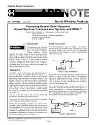
Circuit Ga in = V OH(MIN) – V OL(MAX)2 ⋅ VIN(MAX)Eq. 1.15Under these operating conditions, the differential output voltage of theinstrumentation amplifier circuit is now measured relative to V REF and not toGND. Thus, negative full-scale input signals produce output voltages near A2’s V OL ,and positive full-scale signals produce output voltages near A2’s V OH . Therefore,the circuit's input common-mode range and output dynamic range are optimized interms of the desired circuit gain and amplifier output voltage characteristics.For minimal impact of amplifier output load currents on V OH and V OL , circuitresistor values should be greater than 10kohm in most single-supply applications.Thus, Equations 1.11, 1.14, and 1.15 can all be used to design accurate andrepeatable two op amp instrumentation amplifier circuits with single-supply/rail-torailoperational amplifiers.One fundamental limitation of the two operational amplifier instrumentationcircuit is that since the two amplifiers are operating at different closed-loop gains(and thus at different bandwidths), there will be generally poor AC common-moderejection without the use of an AC CMR trim capacitor. For optimal AC CMRperformance, a trimming capacitor should be connected between the invertingterminal of A1 to ground.A TWO OP AMP, FET-INPUT INSTRUMENTATIONAMPLIFIERFigure 1.9 illustrates a two op amp instrumentation amplifier using the AD822, adual JFET-input, rail-to-rail output operational amplifier. The output offset voltageis set by V REF .15

A SINGLE-SUPPLY, PROGRAMMABLE, FET-INPUTINSTRUMENTATION AMPLIFIERFigure 1.9Dual operational amplifiers, like the AD822, make these types of instrumentationamplifiers both cost- and power-efficient. In fact, when operating on a single, +3 Vsupply, total circuit power consumption is less than 3.5mW. The AD822’s 2pA biascurrents minimize offset errors caused by unbalanced source impedances.Circuit performance is enhanced dramatically by the use of a matched resistornetwork. A thin-film resistor array sets the circuit gain to either 10 or 100 througha DPDT (double-pole, double-throw) switch. The array’s resistors are laser-trimmedfor a ratio match of 0.01%, and exhibit a maximum differential temperaturecoefficient of 5ppm/°C. Note that in this application circuit, the fifth gain-settingresistor is not used. The use of this gain trim resistor would introduce serious gainand linearity errors due to the resistance of the double-pole, double-throw switches.A performance summary and transient response of this instrumentation amplifier isshown in Figure 1.10. Note that the small-signal bandwidth of the circuit isindependent of supply voltage, and that the rail-to-rail output pulse response is wellbehaved.For greater bandwidth at the expense of higher supply current, thefunctionally similar AD823 can also be used.16

PERFORMANCE SUMMARY OF AD822 IN-AMPFigure 1.10THE THREE OP AMP INSTRUMENTATION AMPLIFIERTOPOLOGYFor the highest precision and performance, the three op amp instrumentationamplifier topology is optimum for bridge and other offset transducer applicationswhere high accuracy and low nonlinearity are required. This is at the expense ofadditional power consumption over the two op amp instrumentation circuit (3amplifiers versus 2 amplifiers). Furthermore, like the two op amp configuration, theinput amplifiers can use one dual op amp for tight matching of input offset voltagematching, input bias current, and open-loop gain. Or, a single quad operationalamplifier can be used for the whole circuit, including a reference voltage buffer, ifrequired.Single-supply/rail-to-rail amplifiers can be used in this topology, like that shown fortwo op amp designs, if the output characteristics of the single-supply/rail-to-railamplifiers are understood. As shown in Figure 1.11, a generalized, comprehensiveanalysis of the structure will illustrate the behavior of the nodal voltages andamplifier output currents as functions of the applied common-mode input voltage(V CM ), the applied differential (signal) voltage (V IN ), and the output referencevoltage (V REF ). As shown in Eq. 1.16 through 1.27, the nodal analysis was carriedout for positive-input differential voltages; because of the symmetry in the circuit,the expressions for the nodal voltages and amplifier output currents carried out fornegative-input differential voltages are identical.17

THE UBIQUITOUS 3 OP AMP INSTRUMENTATIONAMPLIFIER IN SINGLE-SUPPLY APPLICATIONSFigure 1.11Using half-circuit concepts and the principle of superposition, the signal voltageapplied to the non-inverting terminal of A1 is set to zero. Since the input signal isapplied to the non-inverting terminal of A2, then an expression for the outputvoltage of amplifier A1 (node A) for positive, differential input signals is given by Eq.1.16:V A =(–V IN +R1) ⎛ RG+ V CM⎝ ⎜ ⎞⎟ Eq. 1.16⎠Since the voltage at the inverting input of A1 must equal the voltage at its noninvertingterminal, then an expression for the voltage at amplifier A1’s invertingterminal (node B) is given by Eq. 1.17:V B = V CM Eq. 1.17In a similar manner, the voltage at A2’s inverting terminal must equal the voltageon A2’s non-inverting terminal:V C = V IN ++ V CM Eq. 1.18The expression for the output voltage of A2 (node D) shows that it is dependentupon both the input signal and the applied input common-mode voltage:V D =(V IN +⎛ R2 ⎞) ⎜1 + ⎟RG+ V CM Eq. 1.19⎝ ⎠At this point, it is worth noting the behavior of the nodal voltages of the inputamplifiers as functions of the applied differential input voltage and the inputcommon-mode voltage. From Eqs. 1.17 and 1.18, the common-mode component of18

the current through the gain setting resistor, R G ,is zero – the input stages simplybuffer the applied input common-mode voltage. In other words, the input stagecommon-mode gain is unity.On the other hand, the full differential input voltage appears across R G . In fact, Eq.1.16 shows that A1 multiplies and inverts the input differential voltage by a factor of(– R1/R G ), while Eq. 1.19 shows that A2 multiplies the input voltage by a factor of(1+ R1/R G ). For the case where the output subtractor stage is configured for a gainof 1, all the differential gain is set in the input stage. Therefore, the ratio of R1 toR G (or R2 to R G ) could be as small as 1:1 or as large as 5000:1. Therefore, to avoidinput amplifier output voltage saturation requires an upper and a lower bound beplaced on the total input voltage (defined to be common-mode plus differential-modevoltages). These bounds are set by the gain of the instrumentation amplifier and theoutput high and low voltage limits of the amplifier. The lower bound on the totalapplied input voltage is given by Eq. 1.20:⎛V IN(TOTAL) > V OL(MAX) + G-1 ⎞⎜ ⎟ (V ) Eq. 1.20⎝ 2 ⎠ IN +An upper bound on the total input voltage can be determined in a similar fashionand is also dependent on the circuit gain and the amplifier’s minimum output highvoltage:⎛V IN(TOTAL) < V OH(MIN) – G+ 1 ⎞⎜ ⎟ (V ) Eq. 1.21⎝ 2 ⎠ IN +For example, if a rail-to-rail operational amplifier exhibited a V OL(MAX) equal to10mV and a V OH(MIN) equal to 4.95V, and if the application required a circuit gainof 10 for a 1V full-scale output, then the total input voltage range would be boundedby:0.46 V < V IN(TOTAL) < 4.4 VTherefore, for the three op amp instrumentation circuit, the total applied inputvoltage range expressed in terms of circuit gain and amplifier output voltage limitsis given by:⎛V OL(MAX) + G-1 ⎞⎛(V ) < V2 IN + IN(TOTAL) < V OH(MIN) – G+1 ⎞⎜ ⎟⎜ ⎟ (V )⎝ ⎠⎝ 2 ⎠ IN +Eq. 1.2219

Since the non-inverting input of the subtractor amplifier A3 determines the voltageon its inverting terminal, an expression for the voltages at Nodes E and F is givenby Eq. 1.23:R6 R2V E = V F =(V IN + R4 + R6 RG+ V R6CMR4 + R6+ V R4) ⎛ ⎝ ⎜ ⎞⎛⎞ ⎛ ⎞ ⎛ ⎞⎟ ⎜1+ ⎟ ⎜ ⎟⎠REF ⎜ ⎟⎝ ⎠ ⎝ ⎠ ⎝ R4 + R6⎠Eq. 1.23For the case where R3, R4, R5, and R6 are all equal to R (typically the case forinstrumentation amplifier gains greater than or equal to 1), then these nodalvoltages will set up at one-half the applied output voltage reference (V REF ) and atone-half the applied input common-mode voltage (V CM ). Furthermore, thecomponent due to the amplified differential input signal is also attenuated by afactor of two. Finally, Eq. 1.24 shows an expression for the circuit’s output voltage inits familiar form for R4 = R3 and R6 = R5:R5 2R1V OUT =(V ) ⎛ IN + ⎝ ⎜ ⎞⎛⎞⎟ ⎜1 + ⎟R3⎠RG+ V REFEq. 1.24⎝ ⎠From Eq. 1.24, the circuit output voltage is only a function of the amplified inputdifferential voltage and the output reference voltage. Provided that R4 = R3 and R6= R5, the component of the output voltage due to the applied input common-modevoltage is completely suppressed. The only remaining error voltage is that due tothe finite CMR of A3 and the ratio match of R3 to R5 and R4 to R6. Also, in theabsence of either an input signal or an output reference voltage, A3’s output voltageis equal to zero; in a single-supply application where rail-to-rail output amplifiers areused, it is equal to V OL .To complete the analysis of this instrumentation circuit, expressions for operationalamplifier output stage currents have been developed and are shown in Eqs. 1.25through 1.27:⎛I OA1 = V IN +⎞ ⎡⎛R1 ⎞ R3 R2 R41+ + 1+ + V REF -VCM⎜⎝ R3 ⎟ ⎜ ⎟ ⎛⎠ ⎝ RG ⎠⎝ ⎜ ⎞ ⎛ ⎞⎟ ⎜ ⎟ ⎛ R1 ⎠ ⎝ RG ⎠ ⎝ ⎜ ⎞ ⎤⎢⎟ ⎥⎣⎢R4 + R6⎠⎦⎥R3⎛ R4 ⎞⎜ ⎟⎝ R4 + R6⎠Eq. 1.25⎧⎪I OA2 = (–V 1 + R2 1IN + RG R2 + 1R4 – 1 R6) ⎛ –⎝ ⎜ ⎞ ⎡⎛ ⎞⎤⎨ ⎟ ⎢⎜ ⎟⎠ ⎣R4 ⎝ R4 + R6⎠⎥⎩⎪⎦⎛⎜⎝1 ⎞ ⎫⎪⎟ ⎬R2⎠⎭⎪+ V REF – VCMR4 + R6Eq. 1.2620

I OA3 =−(V IN +) ⎛ R13 + R5 RG + R5 2⋅ R1 ⋅R5⎞+R3 R3 RG + V CM − VREF⎜⎟R ⎝⋅ ⎠ R3 + R5Eq. 1.27Recall in the analysis of the two-amplifier instrumentation circuit that amplifieroutput stage currents were defined to be positive, if current flow is into the device,the amplifier is sinking current. Conversely, if the nodal analysis shows that outputcurrents are negative quantities, then current flow is out of the amplifier, and theamplifier is sourcing current.Equation 1.25 illustrates that A1’s output stage must be able to sink current as afunction of the applied differential input voltage and the output reference voltage.On the other hand, A1’s output stage is required to source current throughout theapplied common-mode voltage. In the single-supply case where the circuit isrequired to sense small differential signals near ground, Eq. 1.16 and Eq. 1.25 bothillustrate that A1’s output stage is required to sink current while trying to maintaina more negative output voltage than its own negative supply. A1 cannot sustainthis operating point, and thus is forced into output saturation.As shown in Eq. 1.26, A2’s output stage sources current for positive input signalvoltages with no differential nor common-mode voltage constraints placed upon itsoutput by Eq. 1.19. A3’s output stage is also required to source current around itsfeedback resistor as a function of the positive input differential voltage. Note,however, that as a function of the applied common-mode voltage, it is required tosink current. Unfortunately Eq. 1.24 showed that in the absence of an input signal,A3’s output stage can be forced into saturation, trying to sink current whilemaintaining its output voltage at A3’s V OL .To circumvent circuit topological and amplifier output voltage limitations, the resultsshown in Eq. 1.14 and Eq. 1.15 for the two op amp instrumentation circuit applyequally well here. The output reference voltage is chosen in the middle of A1 andA2’s output voltage swing:V REF = V OH(MIN) + V OL(MAX)Eq. 1.142Similarly, output signal dynamic range and output SNR are maximized if the gain ofthe instrumentation circuit is set according to Eq. 1.15:Circuit Ga in = V OH(MIN) – V OL(MAX)2 ⋅ VIN(MAX)Eq. 1.15Under these operating conditions, the differential output voltage of theinstrumentation amplifier circuit is now measured relative to V REF and not toGND. Thus, negative full-scale input signals yield output voltages near A3’s V OL ,and positive full-scale signals produce output voltages near A3’s V OH . Thus, circuitinput common-mode range and output dynamic range are optimized in terms of thedesired circuit gain and amplifier output voltage characteristics.21

For minimal impact on V OH and V OL due to amplifier output load currents, circuitresistor values should be greater than 10kohm in single-supply applications. Thus,Equations 1.22, 1.14, and 1.15 can all be used to design accurate and repeatablethree op amp instrumentation amplifier circuits with single-supply/rail-to-railoperational amplifiers.A COMPOSITE, SINGLE-SUPPLY INSTRUMENTATIONAMPLIFIER [3]As it has been shown throughout this chapter, operation of high performance linearcircuits from a single, low-voltage supply (5V or less) is a common requirement.While there are many precision single supply operational amplifiers (some rail-rail),such as the OP213, the OP291, and the OP284, and some good single-supplyinstrumentation amplifiers, such as the AMP04 and the AD626 (both covered later),the highest performance instrumentation amplifiers are still specified for dualsupplyoperation.One way to achieve both high precision and single-supply operation takesadvantage of the fact that several popular transducers (e.g. strain gauges) providean output signal centered around the (approximate) mid-point of the supply voltage(or the reference voltage), where the inputs of the signal conditioning amplifierneed not operate near “ground” or the positive supply voltage.Under these conditions, a dual-supply instrumentation amplifier referenced to thesupply mid-point followed by a “rail-to-rail” operational amplifier gain stage providesvery high DC precision. Figure 1.12 illustrates one such high-performanceinstrumentation amplifier operating on a single, +5V supply. This circuit uses anAD620 low-cost precision instrumentation amplifier for the input stage, and anAD822 JFET-input dual rail-to-rail output operational amplifier for the output stage.A PRECISION SINGLE-SUPPLY INSTRUMENTATIONAMPLIFIER WITH RAIL-TO-RAIL OUTPUTFigure 1.1222

In this circuit, R1 and R2 form a voltage divider which splits the supply voltage inhalf to +2.5V, with fine adjustment provided by a trimming potentiometer, P1. Thisvoltage is applied to the input of an AD822 which buffers it and provides a lowimpedancesource needed to drive the AD620’s output reference port. The AD620’sREFERENCE input has a 10kohm input resistance and an input signal current ofup to 200µA. The other half of the AD822 is connected as a gain-of-3 inverter, sothat it can output ±2.5V, “rail-to-rail,” with only ±0.83V required of the AD620. Thisoutput voltage level of the AD620 is well within the AD620’s capability, thusensuring high linearity for the “dual-supply” front end. Note that the final outputvoltage must be measured with respect to the +2.5V reference, and not to GND.The general gain expression for this composite instrumentation amplifier is theproduct of the AD620 and the inverting amplifier gains:GAIN⎛ 49. 4kΩ ⎞= +RF⎜ ⎟ ⎛ ⎝ RG ⎠⎝ ⎜⎞1 ⎟RI ⎠Eq. 1.28For this example, an overall gain of 10 is realized with R G = 21.5kohm (closeststandard value). The table (Figure 1.13) summarizes various R G /gain values.In this application, the total input voltage applied to the inputs of the AD620 can beup to +3.5V with no loss in precision. For example, at an overall circuit gain of 10,the common-mode input voltage range spans 2.25V to 3.25V, allowing room for the±0.25V full-scale differential input voltage required to drive the output ±2.5V aboutV REF .The inverting configuration was chosen for the output buffer to facilitate systemoutput offset voltage adjustment by summing currents into the buffer’s feedbacksumming node. These offset currents can be provided by an external DAC, or froma resistor connected to a reference voltage.The AD822 rail-to-rail output stage exhibits a very clean transient response (notshown) and a small-signal bandwidth over 100kHz for gain configurations up to 300.Figure 1.13 summarizes the performance of this composite instrumentationamplifier. To reduce the effects of unwanted noise pickup, a capacitor isrecommended across A2’s feedback resistance to limit the circuit bandwidth to thefrequencies of interest. Also, to prevent the effects of input-stage rectification, anoptional 1kHz filter is recommended at the inputs of the AD620.23

PERFORMANCE SUMMARY OF THE +5V SINGLE-SUPPLYAD620/AD822 COMPOSITE INSTRUMENTATION AMPWITH RAIL-TO-RAIL OUTPUTSFigure 1.13LOW-SIDE AND HIGH-SIDE SIGNAL CONDITIONINGAs previous discussions have shown, single-supply and rail-to-rail operationalamplifiers in two and three op amp instrumentation amplifier circuits imposecertain limits on the usable input common-mode and output voltage ranges of thecircuit. There are, however, many single-supply applications where low- and highsidesignal conditioning is required. For these applications, novel circuit designtechniques allow sensing of very small differential signals at GND or at V POS . Twosuch devices, the AMP04 and AD626, have been designed specifically for theseapplications.As illustrated in Figure 1.14, the AMP04, a single-supply instrumentation amplifier,uses a inverting-mode output gain architecture, where an external resistor, R G(connected between the AMP04’s Pins 1 and 8), is used as the input resistor to A4,and an internal 100kohm thin-film resistor, R1, serves as the output amplifier’sfeedback resistance. Unity-gain input buffers A1 and A2 both serve two functions:they present a high impedance to the source, and provide a DC level shift to theapplied common-mode input voltage of one V BE for amplifiers A3 and A4. As aresult, their output stages can operate very close the negative supply withoutsaturating.The input buffers are designed with PNP transistors that allow the applied commonmodevoltage range to extend to 0V. In fact, the usable input common-mode voltagerange of the AMP04 actually extends 0.25V below the negative supply (although notguaranteed, applied input voltages to any integrated circuit should always remainwithin its total supply voltage range). On the other hand, since the input buffers arePNP stages, the input common-mode voltage range does not include the AMP04’spositive supply voltage. When the inputs are driven within 1V of the positive rail,24

the PNP input transistors are forced into cutoff; and, as a result, input offsetvoltages and bias currents increase, and CMR degrades.SINGLE SUPPLY INSTRUMENTATION AMP HANDLESZERO-VOLTS INPUT AND ZERO-VOLTS OUTPUT (AMP04)Figure 1.14A pulsed-bridge transducer-driver/amplifier illustrates the utility of this low-power,single-supply instrumentation amplifier circuit as shown in Figure 1.15. Commonlyavailable 350ohm strain-gauge bridges are difficult to apply in low-voltage, lowpowersystems for a number of reasons, including the requirements for high bridgedrive currents and high sensitivity. For low-speed measurements, power limitationscan be overcome by operating the bridge in a pulsed-power mode, reading theamplified output on a low-speed, low-duty-cycle basis.25

A LOW POWER, PULSED LOAD CELL BRIDGE AMPLIFIERFigure 1.15In this circuit, an externally generated 800µs TTL/CMOS pulse is applied to theSHUTDOWN input to the REF195, a +5V precision voltage reference. The REF195’sshutdown feature is used to switch between a normal +5V DC output if left open (orat logic HIGH), and a low-power-down standby state (5µA maximum current drain)with the shutdown pin held low. The switched 5V output from the REF195 drivesthe bridge and supplies power to the AMP04. The AMP04 is programmed for a gainof 20 by the 4.99kohm resistor, which should be a stable film type (TCR = 50ppm/°Cor better) in close physical proximity to the amplifier. Dynamic performance of thecircuit is excellent, because the AMP04’s output settles to within 0.5mV of its finalvalue in about 230µs (not shown).This approach allows fast measurement speed with a minimum standby power.Generally speaking, with all active circuitry essentially being switched by themeasurement pulse, the average current drain of this circuit is determined by itsduty cycle. On-state current drain is about 15mA from the 6V battery during themeasurement interval (90mW peak power). Therefore, an 800µs measurementstrobe once per second will dissipate an average of 72µW, to which is added the30µW standby power of the REF195. In any event, overall operation is enhanced bythe REF195’s low-dropout regulation characteristics. The REF195 can operate withsupply voltages as low as +5.4 V and still maintain +5V output operation.If low-frequency filtering is desired, an optional capacitor can be connected betweenpins 6 and 8 of the AMP04. However, a much longer strobe pulse must be used sothat the filter can settle to the circuit’s required accuracy. For example, if a 0.1µFcapacitor is used for noise filtering, then the R-C time constant formed with theAMP04’s internal 100kohm resistor is 10ms. Therefore, for a 10-bit settlingcriterion, 6.9 time constants, or 70ms, should be allowed. Obviously, this will placegreater demands upon system power, so trade-offs may be necessary in the amountof filtering used.26

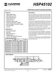
Of course, the amplified bridge output appears only during the measurementinterval, and is valid after 220µs unless filtering is used. During this time, a sampledinputADC (analog-to-digital converter) reads V OUT , eliminating the need for adedicated sample-and-hold circuit to retain the output voltage. If 10-bitmeasurements are sufficient, the 5V bridge drive can also be assumed to beconstant (for 10-bit accuracy), because the REF195 exhibits a ±1mV (±0.02 %)output voltage tolerance. For more accurate measurements, a ratiometric readingof the bridge status can be obtained by reading the bridge drive (V REF ) as well asV OUT .On the other hand, single-supply instrumentation amplifiers, like the AD626, shownin Figure 1.16, exhibit an input stage architecture that allows the sensing of smalldifferential input signals, not only at its positive supply, but beyond it as well. TheAD626 is a differential amplifier consisting of a precision balanced attenuator, a verylow-drift preamplifier (A1), and an output buffer amplifier (A2). It has beendesigned so that small differential signals can be accurately amplified and filtered inthe presence of large common-mode voltages, without the use of any other externalactive or passive components.AD626 SCHEMATIC ILLUSTRATES INPUT PROTECTIONAND SCALING RESISTORS AND ALLOWSINPUT COMMON MODE VOLTAGE UP TO 6 x (Vs - 1V)Figure 1.16The simplified equivalent circuit in Figure 1.16 illustrates the main elements of theAD626. The signal inputs at Pins 1 and 8 are first applied to the dual resistiveattenuators R1 through R4, whose purpose is to reduce the peak common-modevoltage at the inputs of A1. This allows the applied differential voltage to beaccurately amplified in the presence of large common-mode voltages six timesgreater than that which can be tolerated by the actual input to A1. As a result, inputcommon-mode rejection extends to 6×(V s – 1V). The overall common-mode error isminimized by precise laser trimming of R3 and R4, thus giving the AD626 acommon-mode rejection ratio (CMRR) of at least 10,000:1 (80dB).27

To minimize the effect of spurious RF signals at the inputs due to rectification at theinputs to A1, small filter capacitors C1 and C2, internal to the AD626, limit the inputbandwidth to 1MHz.The output of A1 is connected to the input of A2 via a 100kohm resistor (R12) toallow the low-pass filtering to the signals of interest. To use this feature, a capacitoris connected between Pin 4 and the circuit’s common. Equation 1.29 can be used todetermine the value of the capacitor, based on the corner frequency of this low-passfilter:C LP =1( Ω)2π⋅100 k ⋅fLPEq. 1.29where f LP = the desired corner frequency of the low-pass filter, in Hz.The 200kohm input impedance of the AD626 requires that the source resistancedriving this amplifier should be less than 1kohm to minimize gain error. Also, anymismatch between the total source resistance of either input will affect gainaccuracy and common-mode rejection. For example, when operating at a gain of 10,an 80ohm mismatch in the source resistance between the inputs will degrade circuitCMR to 68dB.Output amplifier, A2, operates at a gain of 2 or 20, thus setting the overall,precalibrated gain of the AD626 (with no external components) at 10 or 100. Thegain is set by the feedback network around amplifier A2.The output of A2 uses an internal 10kohm resistor to –V s to “pull down” its output.In single-supply applications where –V s equals GND, A2’s output can drive a10kohm ground-referenced load to at least +4.7V. The minimum nominal “zero”output voltage of the AD626 is 30mV.If pin 7 is left unconnected, the gain of the AD626 is 10. By connecting pin 7 to GND,the AD626’s gain can be set to 100. To adjust the gain of the AD626 for gainsbetween 10 and 100, a variable resistance network can be used between pin 7 andGND. This variable resistance network includes a fixed resistor with a rheostatconnectedpotentiometer in series. The interested reader should consult the AD626data sheet for complete details for adjusting the gain of the AD626. For theseapplications, a ±20% adjustment range in the gain is required. This is due to the onchipresistors absolute tolerance of 20% (these resistors, however, are ratiomatchedto within 0.1%).An example of the AD626 high-side sensing capabilities, Figure 1.17 illustrates atypical current sensor interface amplifier. The signal current is sensed across thecurrent shunt, R s . For reasons mentioned earlier, the value of the current shuntshould be less than 1ohm and should be selected so that the average differentialvoltage across this resistor is typically 100mV. To generate a full-scale outputvoltage of +4V, the AD626 is configured in a gain of 40. To accommodate thetolerance in the current shunt, the variable gain-setting resistor network shown in28

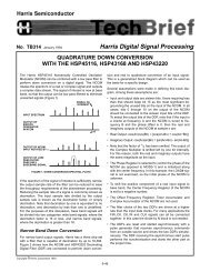
the circuit has an adjustment range of ±20%. Note that sufficient headroom existsin the gain trim to allow at least a 10% overrange (+4.4V).AD626 HIGH-SIDE CURRENT MONITOR INTERFACEFigure 1.17INSTRUMENTATION AMPLIFIER INPUT-STAGERECTIFICATIONA well-known phenomenon in analog integrated circuits is RF rectification,particularly in instrumentation amplifiers and operational amplifiers. Whileamplifying very small signals, these devices can rectify unwanted high-frequency,out-of-band signals. The results are DC errors at the output in addition to thewanted sensor signal. Unwanted out-of-band signals enter sensitive circuitsthrough the circuit's conductors which provide a direct path for interference tocouple into a circuit. These conductors pick up noise through capacitive, inductive,or radiation coupling. Regardless of the type of interference, the unwanted signal isa voltage which appears in series with the inputs.All instrumentation and operational amplifier input stages are either emittercoupled(BJT) or source-coupled (FET) differential pairs with resistive or currentsourceloading. Depending on the quiescent current level in the devices and thefrequency of the interference, these differential pairs can behave as high-frequencydetectors. As it has been shown in [1], this detection process produces spectralcomponents at the harmonics of the interference as well at DC. It is the DCcomponent that shifts internal bias levels of the input stages causing errors, whichcan lead to system inaccuracies. For a complete treatment of this issue, includinganalytical and empirical results, the interested reader should consult Reference [1].Since it is required to prevent unwanted signals and noise from entering the inputstages, input filtering techniques are used for these types of devices. As illustratedin Reference [1], this technique uses an equivalent approach suggested foroperational amplifiers. As shown in Figure 1.18, low-pass filters are used in series29

with the differential inputs to prevent unwanted noise from reaching the inputs.Here, capacitors, C X1 , C X2 , and C X3 , connected across the inputs of theinstrumentation amplifier, form common-mode (C X1 and C X2 ) and differentialmode(C X3 ) low-pass filters with the two resistors, R X . Time constants R X -C X1 andR X -C X2 should be well-matched (1% or better), because imbalances in theseimpedances can generate a differential error voltage which will be amplified.On the other hand, an additional benefit of using a differentially-connectedcapacitor is that it can reduce common-mode capacitive imbalance. This differentialconnection helps to preserve high-frequency AC common-mode rejection. Sinceseries resistors are required to form the low-pass filter, errors due to poor layout(CMR imbalance), component tolerance of R X (input bias current-induced offsetvoltage) and resistor thermal noise must be considered in the design process. Inapplications where the sensor is an RTD or a resistive strain gauge, R X can beomitted, provided the sensor is close to the amplifier.EXTERNAL COMMON-MODE AND DIFFERENTIAL-MODEINPUT FILTERS PREVENT RFI RECTIFICATION ININSTRUMENTATION AMPLIFIER CIRCUITSFigure 1.1830

REFERENCES1. Systems Application Guide, Chapter 1, pg. 21-55, Analog Devices,Incorporated, Norwood, MA, 1993.2. Linear Design Seminar, Section 1, pp. 19-22, Analog Devices,Incorporated, Norwood, MA, 1995.3. Lew Counts, Product Line Director, Advanced Linear Products,Analog Devices, Incorporated, personal communication, 1995.4. Walt Jung, and James Wong, Op amp selection minimizes impact ofsingle-supply design, EDN, May 27, 1993, pp. 119-124.5. E. Jacobsen, and J. Baum, Home-brewed circuits tailor sensor outputsto specialized needs, EDN, January 5, 1995, pp. 75-82.6. Walt Jung, Corporate Staff Applications Engineer, Analog Devices,Incorporated, personal communication, January 27, 1995.7. Walt Jung, Analog-Signal-Processing Concepts Get More Efficient,Electronic Design Analog Applications Issue, June 24, 1993,pp. 12-27.8. C.Kitchin and L.Counts , Instrumentation Amplifier ApplicationGuide, Analog Devices, Incorporated, Norwood, MA, 1991.31