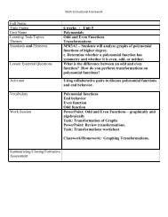
Acquisition Lesson Planning Form - Ciclt.net

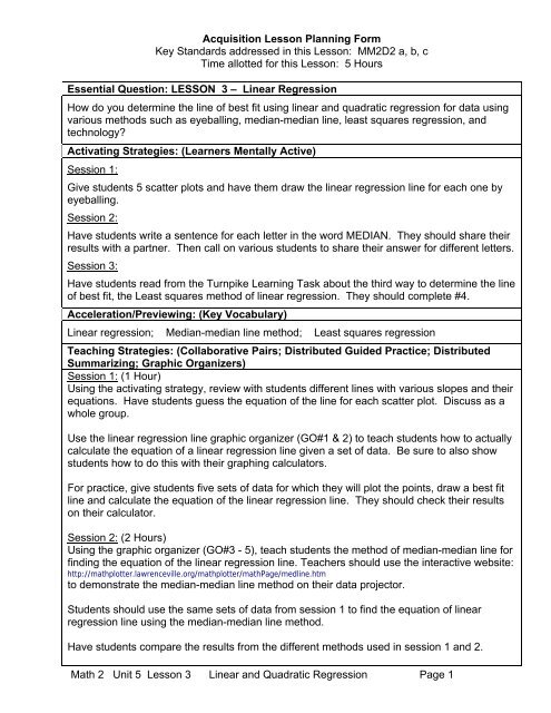
Acquisition Lesson Planning FormKey Standards addressed in this Lesson: MM2D2 a, b, cTime allotted for this Lesson: 5 HoursEssential Question: LESSON 3 – Linear RegressionHow do you determine the line of best fit using linear and quadratic regression for data usingvarious methods such as eyeballing, median-median line, least squares regression, andtechnology?Activating Strategies: (Learners Mentally Active)Session 1:Give students 5 scatter plots and have them draw the linear regression line for each one byeyeballing.Session 2:Have students write a sentence for each letter in the word MEDIAN. They should share theirresults with a partner. Then call on various students to share their answer for different letters.Session 3:Have students read from the Turnpike Learning Task about the third way to determine the lineof best fit, the Least squares method of linear regression. They should complete #4.Acceleration/Previewing: (Key Vocabulary)Linear regression; Median-median line method; Least squares regressionTeaching Strategies: (Collaborative Pairs; Distributed Guided Practice; DistributedSummarizing; Graphic Organizers)Session 1: (1 Hour)Using the activating strategy, review with students different lines with various slopes and theirequations. Have students guess the equation of the line for each scatter plot. Discuss as awhole group.Use the linear regression line graphic organizer (GO#1 & 2) to teach students how to actuallycalculate the equation of a linear regression line given a set of data. Be sure to also showstudents how to do this with their graphing calculators.For practice, give students five sets of data for which they will plot the points, draw a best fitline and calculate the equation of the linear regression line. They should check their resultson their calculator.Session 2: (2 Hours)Using the graphic organizer (GO#3 - 5), teach students the method of median-median line forfinding the equation of the linear regression line. Teachers should use the interactive website:http://mathplotter.lawrenceville.org/mathplotter/mathPage/medline.htmto demonstrate the median-median line method on their data projector.Students should use the same sets of data from session 1 to find the equation of linearregression line using the median-median line method.Have students compare the results from the different methods used in session 1 and 2.Math 2 Unit 5 Lesson 3 Linear and Quadratic Regression Page 1

Session 3: (2 Hours)In pairs, have students complete #5-6 from the learning task. In whole group, discussanswers to question #6.So that students can once again practice all three methods, have them complete #7-12 in thelearning task.Session 4: (1 Hour)Using Traveling on the Turnpike Learning Task Part 2, the students will make a connectionbetween piecewise functions and lines of best fit using least squares regression. Throughteacher guided instruction, the students and teacher will complete #13-22.Session 5: (2 Hours)Quadratic regression…Distributed Guided Practice/Summarizing Prompts: (Prompts Designed to InitiatePeriodic Practice or Summarizing)What is the correlation coefficient?Extending/Refining Strategies:Summarizing Strategies: Learners Summarize & Answer Essential QuestionSession 1:Traveling on the Turnpike Learning Task Part 1 #1-3. Be sure to write the equation of the linebeside the graph.Session 2:From the Turnpike Learning Task in session 1, students should find the equation of the linearregression line using the median-median line method. Draw this line on the same graph fromsession 1. Be sure to write the equation of the line beside the graph.Session 3:Give students a quiz: Students will be given a set of data of which they should plot the points,eyeball the line of best fit, use visual approximation to write an equation of the line, use themedian-median line method to write the equation of the line, and then use technology to findthe equation of the line using the least squares regression method. They should compare thethree equations and describe which one gives the most accurate representation.Session 5:Math 2 Unit 5 Lesson 3 Linear and Quadratic Regression Page 2

GO #1: How do we eyeball a line best fit a scatter plot?There are several lines passing through the scatter plot below.Which one do you think best fits the data?Line 2Line 1Line 3x y1 21 02 22 13 54 45 36 56 77 68 58 8Choose two points on each of the three lines and fine the equation of eachbefore you decide which one fits the best. Show your work below.Math 2 Unit 5 Lesson 3 Linear and Quadratic Regression Page 3

A linear regression line is astraight line thatapproximates the relationshipbetween two variablesrepresented by a set of data●●●●Find the linear regression lineby calculating the slope⎛ y2− y1⎞⎜m=⎟ and using the⎝ x2− x1⎠slope-intercept formy = mx + b of an equation of a( )line. Check with the linearregression on the graphingcalculator.1. Plot the following points on the grid below:(1, 3), (2, 2), (0, 1), (3,4)By eyeballing:Linear Regression Line: y = _____ x + ____Using the graphing calculator:Linear Regression Line: y = _____ x + ____2. Plot the following points on the grid below:(-4, 2), (1, -2), (-3, -1), (-1, 1)By eyeballing:Linear Regression Line: y = _____ x + ____Using the graphing calculator:Linear Regression Line: y = _____ x + ____Math 2 Unit 5 Lesson 3 Linear and Quadratic Regression Page 4

GO #3: How do we find the median-median line from a set ofdata?1 st Divide the points into 3 equal groups.We would have 4 points in each grouphere. If there were 1 extra point, itwould go in the center section. If therewere 2 extra points, 1 would be in eachof the two outside sections.x y1 21 02 22 13 54 25 36 26 77 98 58 8(7.5, 7.5)(4.5, 2.5)2 nd Find the median x-coordinate and the median y-coordinate in each group of points. This point mayor may not be on your graph. For example, in theleft section, the median x-coordinate is 1.5 and themedian y-coordinate is 1.5, so the point you find is(1.5, 1.5) and is marked by a .Math 2 Unit 5 Lesson 3 Linear and Quadratic Regression Page 5

3 rd Draw a line through thetwo points you found in theoutside sections. This linemay or may not pass throughthe original points on thegraph.(7.5, 7.5)(1.5, 1.5)(4.5, 2.5)5 th Draw a line between and parallel tothe two lines just drawn. This new lineshould be 1/3 of the distance from thefirst line to the second line. In otherwords, it should be closer to the linethrough the outside points. This is themedian-median line.4 th Draw a line passingthrough the point youfound in the centersection. This line shouldbe drawn parallel to theline you just drew throughthe outside points. .Math 2 Unit 5 Lesson 3 Linear and Quadratic Regression Page 6

Now that you have found the median-median line, write its equation. Choose two points on theline and use the point-slope formula to write the equation.Median-MedianLineChoosing the points (2, 1) and ((6, 5) on the median-median line, the slope would bem =yx22−−yx11=5 −1=6 − 243.Point-slope Formula:y – y 1 = m(x – x 1 )y – 1 = 34 (x – 2)y – 1 = 34 x - 38y = 34 x - 35is the equation of the median-median line of best fitMath 2 Unit 5 Lesson 3 Linear and Quadratic Regression Page 7

GO #4A median-median line is a linear regression linethat is found by dividing the data into thirds andfinding the median x- and y-value of each third. Twolines are drawn using the medians. The regressionline lies between these.●●●●●●1. Plot the following points on the grid below: (-1, -1), (2, 2), (0, 1), (3, 4), (-2, -3), (-3, -4)2. Divide the data into thirds. Find the three medians.Median1 = (__,__) Median 2 = (__,__) Median 3 = (__,__)3. Find the median-median line by hand.Median-median Line: y = _____ x + ____4. Now find the median-median line using the following formulay3− y1y + y2+ yMedian-median Line Formula y = ax + b,a = , b =x3− x1Median-median Line: y = _____ x + ____− a( x + x + ) 31 3 1 2xAre they the same? Why or why not? ___________________________________________________________________________________________________________Math 2 Unit 5 Lesson 3 Linear and Quadratic Regression Page 83

5. Plot the following points on the grid below: (-1, 0), (0, -1), (2, -1), (-2, 2), (-3, 4), (3, -3)6. Divide the data into thirds. Find the three medians.Median1 = (__,__) Median 2 = (__,__) Median 3 = (__,__)7. Find the median-median line by hand.Median-median Line: y = _____ x + ____8. Find the median-median line using the following formulay3− y1y + yMedian-median Line Formula y = ax + b,a = , b =x3− x1Median-median Line: y = _____ x + ____− a( x + x + ) 31 2+ y31 2x3Math 2 Unit 5 Lesson 3 Linear and Quadratic Regression Page 9

GO #5A least squares regression line minimizes the sum of the squares of the verticaldistances between the data points and any possible regression line.Find the linear regression line by using the graphing calculator.1. Plot the following points on the grid below: (1, 3), (2, 2), (0, 1), (3,4)Linear Regression Line: y = _____ x + ____2. Plot the following points on the grid below: (-4, 2), (1, -3), (0, -1), (-1, 1)Linear Regression Line: y = _____ x + ____Math 2 Unit 5 Lesson 3 Linear and Quadratic Regression Page 10

Traveling on the Turnpike Learning Task – Part IExamine the toll schedule given by the Ohio Turnpike Commission that is attached to this task.In this task, we will explore the relationship between the distance you travel (based on thenumbers of the exits at which you enter and leave the turnpike) and the amount of the toll.1. Suppose you get on the turnpike at Sandusky-Norwalk. Select five exits whose exitnumbers are larger than 118 (the Sandusky-Norwalk exit number). For the five exits youselect, graph the five ordered pairs of the form (exit #, toll).2. The points in the data set you selected for Item 1 are not all on the same line, but the trendof the data could be approximated by a line. Our goal is to write a linear function whosegraph provides a “line of best fit” to the points in the scatter plot. Look at the five datapoints you chose and plotted, and then decide where to draw a line that, in your opinion,best approximates all of the data points. Draw the line on your plot, and explain the reasonfor your choice of line.3. Now calculate the equation of the linear regression line based on the graphic organizer intoday’s lesson.Data Set 1 Data Set 2Exit numbersToll Fee ($)Exit numberslarger than exit 118larger than exit 118 Toll Fee ($)135 1.00through exit 215140 1.25135 1.00142 1.50151 2.00145 1.75173 3.50151 2.00193 4.75215 6.00yxMath 2 Unit 5 Lesson 3 Linear and Quadratic Regression Page 11

The third way to determine a line of best fit is using the least squares method of linearregression. The least squares method finds the line that minimizes the sum of the squares ofthe vertical distances from data points to points on the line. We will use technology to findleast squares regression lines. The various technological tools that are available use statisticalformulas to find the slope and y-intercept of this line. Interested students may want to find outmore about these formulas, but our focus in this task is learning characteristics of the leastsquares regression line and comparing it to visual and median-median regression lines.4. Use the least squares regression capabilities of your graphing utility to determine a line ofbest fit for your five data points. Graph this new line on the plot with your data and previousbest-fit lines.5. The least squares regression line is the line that minimizes the sum of the squares of thevertical distances between the data points and the approximation line. All otherapproximation lines have a greater sum of squares of vertical distances between datapoints and the approximation line. To verify this property, at least to verify it for the threeapproximation lines you have created, make three tables using the format indicated below– one for each proposed line of best fit (visual approximation, median-median, leastsquares regression) – and then compare the sums of the vertical distances and the sums ofthe squares of the vertical distances.Exit # Toll Predicted toll fromthe approximationline (using visualapproximation)Vertical distancebetween point forpredicted toll andpoint for actualtollSquare of thevertical distancebetween data pointand approximationpointSumExit # Toll Predicted toll fromthe approximationline (usingmedian-medianline)Vertical distancebetween point forpredicted toll andpoint for actualtollSquare of thevertical distancebetween data pointand approximationpointSumMath 2 Unit 5 Lesson 3 Linear and Quadratic Regression Page 12

Exit # Toll Predicted toll fromthe approximationline (using leastsquares, Item 4)Vertical distancebetween point forpredicted toll andpoint for actualtollSquare of thevertical distancebetween data pointand approximationpointSum6. The median-median method of linear regression is based on finding the median values ofdata points. Calculating the least squares method by hand requires using means andstandard deviations. From what you already know about medians and means as measuresof central tendency, what might be one reason to use the median-median line instead of themore common least squares regression line?7. Now, let’s look at the equation for the tolls if we get on the turnpike at Exit 118 and drove inthe other direction. Select five exits whose exit numbers are smaller than 118 (theSandusky-Norwalk exit number). For the five exits you select, graph the five ordered pairsof the form (exit #, toll).Data Set 3 Data Set 4Exit numbersExit numbersToll Fee ($)less than exit 118less than exit 118 Toll Fee ($)110 0.50through exit 291 1.75110 0.5081 2.2581 2.2571 3.0052 4.0064 3.2525 5.752 7.258. Find a visual regression of line for the five data points you selected in Item 7, and draw theline on your scatter plot.yx9. CalculatMath 2 Unit 5 Lesson 3 Linear and Quadratic Regression Page 13

e the median-median line for the five data points you selected in Item 7 and then checkyour results using technology. Draw this line on the same graph with your data points andthe line you found by visual linear regression.10. Using appropriate technology, determine the least squares regression line for the five datapoints you selected in Item 7 and draw it on the plot with your data and previous best-fitlines.11. Consider your least squares regression lines from Items 4 and 10. For each line, round theslope to three decimal places and interpret the rounded value in the context of this problem.Explain how you arrive at your interpretation.12. Consider your least squares regression lines from Item 10 again. Does the y-intercepthave a contextual meaning? If so, what does it represent?Math 2 Unit 5 Lesson 3 Linear and Quadratic Regression Page 14

Traveling on the Turnpike Learning Task – Part 2Our next goal is to find a function that models the toll schedule whenever we begin at theSandusky-Norwalk exit and travel in either direction. For this part we use two least squaresregression lines, one calculated for the points corresponding to all the exits from 118 to 215and the other calculated for the points corresponding to all the exits from 2 to 118.13. The least squares regression line for the data set of all ordered pairs of the form (exit #, toll)for the exits from 118 to 215 is given byy = 0.0629011x – 7.46324.a. Use technology to graph this least squares regression line.b. Find the x-intercept of the line.14. The least squares regression line for the data set of all ordered pairs of the form (exit #, toll)for the exits from 2 to 118 is given byy = – 0.0621573x + 7.34057.a. Use technology to graph this least squares regression line..b. Find the x-intercept of the line.15. We want to find a function that models the toll schedule whenever we begin at theSandusky-Norwalk exit and travel in either direction.a. How should the graphs of the linear functions from Items 13 and 14 be restricted so thatthe graphs can be combined to form a single piecewise function T that models the tollschedule for Ohio Turnpike users who start at the Sandusky-Norwalk exit?b. Graph the piecewise function T from part a in a viewing window with −25 ≤ x ≤225and−10 ≤ y ≤10. If possible, use a graphing utility that allows you to graph piecewisefunctions. Otherwise, graph by hand to include the required graphing window.c. Write the definition of the piecewise function T graphed in part b.Math 2 Unit 5 Lesson 3 Linear and Quadratic Regression Page 15

16. The graph above for Item 15 may remind you of the graph of the absolute value function,which you first encountered in Unit 1 of Mathematics I. The absolute value function is apiecewise function, and its definition can be written in a piecewise format.a. Draw the graph of ( x) xf = using a viewing window with − 5 ≤ x ≤ 5 .b. Identify the pieces of the function f that could be defined using a linear function, andthen list each linear function and the domain restriction needed to make a part of thegraph of f.FunctionDomainc. Combine the pieces listed in part b to write the absolute value function as a piecewisefunction.17. In your previous work with functions, you have explored the effects of transformations onthe graphs of functions. This item asks you to recall some of this information.a. Explain how the function g graphed at the right can be obtained by stretches and shiftsf x = x .of the absolute value function, ( )b. Write a formula for g(x) as a transformation of the absolute value function.c. Write a piecewise definition for the function g.18. We noted that the graph of the function T from Item 15 is similar to the graph of theabsolute value function. We can approximate T using transformations of the absolute valueMath 2 Unit 5 Lesson 3 Linear and Quadratic Regression Page 16

function. We’ll name this approximation of T by a translation of the absolute value functionto be the function S.a. Where should the vertex of the graph of the function S be located? Why?b. One of the characteristics of the absolute value functions is its symmetry. What kind ofsymmetry does the absolute value function have and what symmetry should the graphof S have? Why?c. Consider both parts of the toll graph T. Determine a vertical stretch for the absolutevalue function that you think will produce a function S to best approximate T. Explainyour choice.d. Based on your answers to parts a – c of this item, write a formula for a function S that isobtained by transformation of the absolute value function and, in your opinion, bestapproximates the toll function T.e. How well do you think the function S models the actual data from the Ohio Turnpikeschedule of tolls and why?For the remainder of this task, we will focus on the function S and use it to analyze additionalinformation about tolls while learning more about absolute value functions.19. Describe how you would use your function S from Item 18 to determine the amount of thetoll if a new exit were added between two existing exits. Choose a location to add an exitbetween two existing exits and test your strategy. Where did you place the exit, and howmuch was the toll? 1 Explain if your prediction is reasonable.20. We notice in the toll schedule that exits 151 and 152 have the same toll, $2.00. Now thatwe have a process for finding the toll at future new exits, we could use the underlying idea1 Question adapted from the NCTM Illuminations lesson “Taking Its Toll.” The entire activity can be found athttp://illuminations.nctm.org/LessonDetail.aspx?ID=L571 .Math 2 Unit 5 Lesson 3 Linear and Quadratic Regression Page 17

to ask new questions such as, “What are all the possible exits that would have a toll ofexactly $2.00 if we used the function S to find the initial toll approximation?”a. Based on the process from Item 19, for what toll values predicted by the function Swould we set the toll at $2.00?b. Use the graph of the function S to find all the possible exit numbers for which theprocess of Item 19 would yield a toll of exactly $2.00? Explain your process.21. Using the graph to determine the possible exits that correspond to a particular toll predictedby the function S depends on reading the graph with accuracy. In some cases it may bevery difficult to decide if a particular point on the graph of the function S is below, on , orabove the line corresponding to a particular y-value line just by examining the graph. Forthis reason, we need an algebraic method to find the x-value of any points with a particulary-value when the function is an absolute value function. We’ll explore the method with asimpler absolute value function and then return to our function S.h x = x−− sucha. uppose that we want to find all points on the graph of the function ( ) 6 3 7that h( x ) = 8 . What equation do we need to solve?b. How can we write the formula for the function h as a piecewise function?c. Use the piecewise rule for h to replace the one equation given as the answer for part awith two different equations to solve, and then solve the two equations.d. Verify that each of the solutions in part c gives a value of x such that h( x ) = 8 .22. Now we ask “For what exits, current or future, is the toll on the Ohio Turnpike $5.00 orgreater?”.Math 2 Unit 5 Lesson 3 Linear and Quadratic Regression Page 18

a. Use an algebraic method to answer the question, using the function S to find apredicted value of the toll and then rounding as in Item 19.b. Do these solutions agree with the toll schedule?c. Do these solutions agree with the graph?Math 2 Unit 5 Lesson 3 Linear and Quadratic Regression Page 19

Math 2 Unit 5 Lesson 3 Linear and Quadratic Regression Page 20

Orbital Debris Learning TaskWhenever a space shuttle is launched, mission-related debris are released as part of themission. Satellites that have exhausted their missions remain in orbit, and the bodies of manyof the rockets used to launch various spacecraft are still in space. Paint chips off spacecraftcontinue to float in orbit long after the spacecraft has returned to earth. All of these man-madeitems contribute to the debris in orbit about the Earth. The area where orbital debris is mostconcentrated is known as the LEO (low Earth orbit) and consists of space 200 and 2000 kmabove the Earth’s surface. Telecommunications satellites are found in the geostationary orbit,above the LEO; according to the orbital debris specialists, there is little debris in thegeostationary orbit.Orbital debris can collide with current and future spacecraft and with each other. Although allspacecraft collide with small particles during a mission, a collision with a particle 10 cm indiameter (the measure across the widest part) or larger can cause catastrophic damage to acraft.In response to the growing space pollution issue of orbital debris, the United States beganclose monitoring of orbital space debris, and, along with the United Nations, put into effect aplan to reduce the amount of orbital debris produced and left in space each year. In the UnitedStates, a plan for minimizing the creation of new orbital debris was proposed in 1997 andapproved in 2001. One provision of this plan includes engineering space shuttle missions andsatellite launches so that mission-related debris reenters the Earth’s atmosphere and eitherburns up in descent through the atmosphere or falls safely to Earth in an uninhabited area.All debris with a diameter of 10 cm or greater in low Earth orbit and with a diameter of 1 meteror greater in geostationary Earth orbit (GEO) are catalogued by the United States SpaceSurveillance Network. There are also hundreds of thousands of uncataloged smaller particlesin Earth orbit. The work of monitoring and reporting orbital debris is carried out at the NationalAeronautical and Space Administration (NASA) Orbital Debris Program Office at the JohnsonSpace Center in Houston, Texas. Scientists at the Johnson Space Center use sophisticatedmathematical models and complex computer software to track orbiting debris and spacecollisions involving orbital debris. Tracking debris is a complex activity because the debriscount changes so often. Throughout each year, new spacecraft are launched adding rocketbodies and other mission debris, and break-ups and collisions fragment large debris into manysmaller pieces. While these processes add to the debris, some debris that has been in orbitfor a long time falls back into the atmosphere to return to Earth or be burned up on reentry. Inthis task, we will model orbital debris data while we explore additional concepts aboutmodeling data.1. At the beginning of October 1997, there were 8545 man-made objects in Earth orbit. Overseventy percent of these were orbital debris: mission-related discards, rocket bodies, andfragmentation debris from break-ups and collisions. By late September 2006, there were9800 man-made objects in Earth orbit, about seventy percent of which were debris.a. The table below lists the total number of orbital debris, as cataloged by the US SpaceSurveillance Network, for the years listed in the table 2 .2 Data taken from October issues of the Orbital Debris Quarterly Newsletter available online athttp://orbitaldebris.jsc.nasa.gov/newsletter/newsletter.html . According to Nicholas L. Johnson,Math 2 Unit 5 Lesson 3 Linear and Quadratic Regression Page 21

Year 1997 1998 1999 2000 2001 2004 2005 2006Man-made OrbitalDebris (number ofobjects)6166 6132 5980 6134 6092 6307 6480 6791The first man-made object to orbit the Earth was Sputnik 1, launched by the Union ofSoviet Socialist Republics (USSR) on Oct. 4, 1957. The debris totals provided here arefrom dates near the end of the third quarter of each year. Thus, the dates for the datarepresent a whole number of years from the Sputnik 1 launch, and we can simplify ourdata by using the number of years since the launch as the first coordinate. Write pointscorresponding to the data in the table using the form(number of years since Sputnik 1 launch, number of man-made orbital debris).b. Make a scatterplot of the points from part a.c. Explain any trends in the data.One of our topics for this task is consideration of methods for deciding what type of function touse to model a set of data, that is, deciding whether to use a linear model for the data or use amodel based on another type of function, such as a quadratic function. Note that data that arebest modeled by only the increasing, or only the decreasing, part of a quadratic function mayappear linearly related .Statisticians use a number, called the correlation coefficient, as a measure of the extent towhich the data for two variables show a linear relationship. The correlation coefficient, usuallydenoted by r, measures the both the direction and strength of a linear relationship between twovariables.If the relationship between the data for two variables exactly fits a linear function with positiveslope, the correlation coefficient for the set of data is 1. The number 1 is largest possible valuefor a correlation coefficient. A positive correlation coefficient indicates that a linearapproximation of the data would have a positive slope. Thus, when a set of data has a positivecorrelation coefficient, an increase in one variable is associated with an increase in the othervariable, and a decrease in one variable is generally associated with a decrease in the othervariable. The closer a positive correlation coefficient is to 1, the stronger is the linearChief Scientist for Orbital Debris, NASA Johnson Space Center, via email reply in November2008, this data was current at the time of the newsletter printing but some of it was updatedlater because several months or even years may pass before all the data from a satellitefragmentation is detected and cataloged.Math 2 Unit 5 Lesson 3 Linear and Quadratic Regression Page 22

elationship between the variables; the closer a positive correlation coefficient is to 0, theweaker the relationship.If the relationship between the data for two variables exactly fits a linear function with anegative slope, the correlation coefficient is –1. The number –1 is smallest possible value for acorrelation coefficient. A negative correlation coefficient indicates that a linear approximationof the data would have a negative slope. Thus, when a set of data has a negative correlationcoefficient, an increase in the value of one variable is generally associated with a decrease inthe value of the other variable. The closer a negative correlation coefficient is to –1, thestronger the relationship; the closer a negative correlation coefficient is to 0, the weaker therelationship.A correlation coefficient of zero means that there is no linear relationship for the points in theset of data.1 ⎛ x ⎛ ⎞i− x ⎞ y −The formula for correlation coefficient is given by the equation:⎜iyr = ∑⎟⎜⎟ ,n −1⎝ sx ⎠⎝sy ⎠, , x , y are the data points, x is the mean of the x-values, y is thewhere ( x y ), ( x y ), …, ( )1 11 11 1mean of the y-values, sxis the standard deviation of the x-values, and s y is the standarddeviation of the y-values. In this task, you are expected to use appropriate technology, either acalculator or software package, to calculate the correlation coefficient.There is one important caution about correlation coefficient that must be emphasized:a strong correlation, even one with a coefficient of 1 or –1, does not indicate a causalrelationship between the variables. We will explore this caution further in another task.2. Use a calculator or other appropriate technology to find the correlation coefficient, r, foryour data points from Item 1.a. Based on the value of the correlation coefficient, what are the strength (weak,moderate, or strong) and direction (positive or negative) of any linear relationship forthis set of data?b. Using appropriate technology (graphing calculator, Excel, TI-Interactive, etc.), determinethe least-squares regression line for the data.c. Graph the least squares regression line from part b together with a scatterplot of thedata.Math 2 Unit 5 Lesson 3 Linear and Quadratic Regression Page 23

d. How well does the least squares regression line appear to fit the data?e. Find the sum of the squares of the vertical distances between points on the regressionline and the corresponding data points.f. Interpret the slope of your least squares regression line from part b.g. Interpret the y-intercept of your squares regression line from part b.Many data sets studied by scientists and engineers, like the one studied in Items 1 and 2, canbe viewed as functions since each input has a unique output. However, such real-life data areusually not modeled exactly by any function that we can build using basic functions ortransformations of basic functions. However, mathematical models built from transformationsof basic functions can provide useful information about the data. Thus, finding and comparingdifferent models is a useful endeavor.Linear functions are not the only functions we can use to model data. In the “Traveling on theTurnpike” task, you used least squares linear regression to build an absolute value function tomodel that data. In the remainder of this task, we explore using quadratic functions to modeldata, called quadratic regression. Modeling data with other polynomial functions andexponential functions is also possible. Although our study is limited to quadratic regression,we will see concepts the generalize for higher degree polynomials.3. This item explores quadratic regression for the data points from Item 1. Quadraticregression finds the quadratic function that minimizes the sum of the squares of the verticaldistances between points on the quadratic graph and the data points.a. Use a calculator or other appropriate technology to find the quadratic regressionequation for the data.b. Graph the quadratic regression curve from part b together with a scatterplot of the data.Math 2 Unit 5 Lesson 3 Linear and Quadratic Regression Page 24

c. How well does the parabola appear to fit the data?d. Find the sum of the squares of the vertical distances between points on the quadraticregression curve and the corresponding data points.e. Which function, the least squares linear regression or the quadratic regression, providesa better model for the data from Item 1? Explain your answer.f. The data in Item 1 were obtained from the quarterly news letter published by the NASAOrbital Debris Program Office. The newsletter was not published for a period includingthe third quarters of 2002 and 2003 so, for these two years, the count of man-madedebris in Earth orbit at the end of the third quarter was not available. Use your choice ofthe better model (from part e) to predict the amount of debris for these two years..Finding the answers for Item 3, part f is an example of interpolation. Interpolation is used tomake predictions within the domain of values of the independent variable. It is standard to finda regression curve for the purpose of finding one or more interpolated values.Extrapolation is the use of a regression curve to make predictions outside the domain ofvalues of the independent variable. Care must be taken to determine the feasibility ofextrapolation; that is, sufficient evidence should exist that the trend described by theregression curve would continue outside the present domain.4. Consider using your regression models for the data in Item 1 to estimate man-made orbitaldebris during the period 1957 – 1966.a. Discuss whether it is feasible to use your least squares linear regression to extrapolatevalues for 1957 – 1966.Math 2 Unit 5 Lesson 3 Linear and Quadratic Regression Page 25

. Discuss whether it is feasible to use your quadratic regression function to extrapolatevalues for 1957–1966.5. The amount of man-made debris can change in an instant when a satellite breaks apart orthere is a collision among two pieces of debris. Approximately 1500 new debris wereadded in 2007 as a result of the breakup of the Fengyun-1C and Upper AtmosphericResearch Satellites; these events made 2007 the worst ever year for producing new manmadedebris.a. The actual count of man-made debris in Earth orbit at the end of the third quarter of2007 was 9250. State the error in using your linear and quadratic models to predict thecount of man-made debris in Earth orbit at the end of the third quarter of 2007?b. The actual count of man-made debris in Earth orbit at the end of the third quarter of2008 was 9661. State the error in using your linear and quadratic models to predict thecount of man-made debris in Earth orbit at the end of the third quarter of 2008?c. If you found a new linear or quadratic regression function using the data from parts aand b above as well as the data from Item 1, part a, would you be confident in usingyour model above to predict the amount of man-made debris in Earth orbit for 2010?Explain.Math 2 Unit 5 Lesson 3 Linear and Quadratic Regression Page 26

6.1990 101995 192000 282005 40a. Based on 4a and your regression curves and plots in problem 2, which curve is a better fitfor the data? Explain your answer.b. Use your choice from 4b to predict the cumulative numberof LEO collisions in 2010.Math 2 Unit 5 Lesson 3 Linear and Quadratic Regression Page 27

Causation versus Correlation Learning TaskSTATS is a non-profit, non partisan research organization affiliated with George MasonUniversity. The following is reproduced from their website (http://www.stats.org/faq_vs.htmOne of the most common errors we find in the press is the confusion between correlation andcausation in scientific and health-related studies. In theory, these are easy to distinguish — anaction or occurrence can cause another (such as smoking causes lung cancer), or it cancorrelate with another (such as smoking is correlated with alcoholism). If one action causesanother, then they are most certainly correlated. But just because two things occur togetherdoes not mean that one caused the other, even if it seems to make sense.Unfortunately, our intuition can lead us astray when it comes to distinguishing betweencausality and correlation. For example, eating breakfast has long been correlated with successin school for elementary school children. It would be easy to conclude that eating breakfastcauses students to be better learners. It turns out, however, that those who don’t eat breakfastare also more likely to be absent or tardy — and it is absenteeism that is playing a significantrole in their poor performance. When researchers retested the breakfast theory, they foundthat, independent of other factors, breakfast only helps undernourished children perform better.Many many studies are actually designed to test a correlation, but are suggestive of “reasons”for the correlation. People learn of a study showing that “girls who watch soap operas are morelikely to have eating disorders” — a correlation between soap opera watching and eatingdisorders — but then they incorrectly conclude that watching soap operas gives girls eatingdisorders.In general, it is extremely difficult to establish causality between two correlated events orobservances. In contrast, there are many statistical tools to establish a statistically significantcorrelation.There are several reasons why common sense conclusions about cause and effect might bewrong. Correlated occurrences may be due to a common cause. For example, the fact that redhair is correlated with blue eyes stems from a common genetic specification which codes forboth. A correlation may also be observed when there is causality behind it — for example, it iswell-established that cigarette smoking not only correlates with lung cancer, but actuallycauses it. But in order to establish cause, we would have to rule out the possibility thatsmokers are more likely to live in urban areas, where there is more pollution — or any otherpossible explanation for the observed correlation.In many cases, it seems obvious that one action causes another. However, there are alsomany cases when it is not so clear (except perhaps to the already-convinced observer). In thecase of soap-opera watching anorexics, we can neither exclude nor embrace the hypothesisthat the television is a cause of the problem — additional research would be needed to make aconvincing argument for causality. Another hypothesis is that girls inclined to suffer poor bodyimage are drawn to soap operas on television because it satisfies some need related to theirpoor body image. Yet another hypothesis is that neither causes the other, but rather there is acommon trait — say, an overemphasis on appearance by the girls’ parents — that causes bothan interest in soap operas and an inclination to develop eating disorders. None of theseMath 2 Unit 5 Lesson 3 Linear and Quadratic Regression Page 28

hypotheses are tested in a study that simply asks who is watching soaps and who isdeveloping eating disorders, and finding a correlation between the two.How, then, does one ever establish causality? This is one of the most daunting challenges ofpublic health professionals and pharmaceutical companies. The most effective way of doingthis is through a controlled study. In a controlled study, two groups of people who arecomparable in almost every way are given two different sets of experiences (such one groupwatching soap operas and the other game shows), and the outcome is compared. If the twogroups have substantially different outcomes, then the different experiences may have causedthe different outcome.There are obvious ethical limits of controlled studies – it would be problematic to take twocomparable groups and make one smoke while denying cigarettes to the other in order to seeif cigarette smoking really causes lung cancer. This is why epidemiological (or observational)studies are so important. These are studies in which large groups of people are followed overtime, and their behavior and outcome is also observed. In these studies, it is extremely difficult(though sometimes still possible) to tease out cause and effect, versus a mere correlation.Typically, one can only establish correlation unless the effects are extremely notable and thereis no reasonable explanation that challenges causality. This is the case with cigarette smoking,for example. At the time that scientists, industry trade groups, activists and individuals weredebating whether the observed correlation between heavy cigarette smoking and lung cancerwas causal or not, many other hypotheses were considered (such as sleep deprivation orexcessive drinking) and each one dismissed as insufficiently describing the data. It is now awidespread belief among scientists and health professionals that smoking does indeed causelung cancer.When the stakes are high, people are much more likely to jump to causal conclusions. Thisseems to be doubly true when it comes to public suspicion about chemicals and environmentalpollution. There has been a lot of publicity over the purported relationship between autism andvaccinations, for example. As vaccination rates went up across the United States, so didautism. However, this correlation (which has led many to conclude that vaccination causesautism) has been widely dismissed by public health experts. The rise in autism rates is likely todo with increased awareness and diagnosis, or one of many other possible factors that havechanged over the past 50 years.In general, we should all be wary of our own bias; we like explanations. The media oftenconcludes a causal relationship among correlated observances when causality was not evenconsidered by the study itself. Without clear reasons to accept causality, we should onlyaccept correlation. Two events occurring in close proximity does not imply that one caused theother, even if it seems to makes perfect sense.Do the following activities with the aid of research on the topic of correlation versuscausation. An Internet search on this topic will produce a wealth of examples to consider.Most introductory statistics textbooks have a section on the topic.1. Find one example, or collect data to create an example of your own, of a strong correlation(either positive or negative) between variables where the idea that either one causes theother is clearly not reasonable.a) Describe the two variables that are correlated.Math 2 Unit 5 Lesson 3 Linear and Quadratic Regression Page 29

) Give the correlation coefficient or evidence to support the claim that there is a strongcorrelation.c) Write a sentence making the claim that one variable causes the second.d) Give an explanation of why the correlation may exist.e) Make a bibliography of all sources used.2. Find an example of a topic of current public interest where there is a correlation betweentwo quantities, call them A and B, that has been interpreted, at least in some media, as Acausing B.a) State the claim that A causes B providing the source of the claim and explanations ofterms as necessary.b) Discuss possible reasons that there may be a correlation without A actually causing B,such as a third variable C related to A and B.c) Make a bibliography of all sources used.Math 2 Unit 5 Lesson 3 Linear and Quadratic Regression Page 30

View Tube Learning TaskThis learning task requires you to work in pairs to collect and then analyze data.Supplies needed by each pair of students:• a cardboard tube, such as a paper towel or gift roll• yard stick or meter stick• masking tape• marker• strips of colored paperSet up for data collection:• Choose one student to be the viewer and one to be the recorder.• Choose a wall that is unobstructed for several feet in front of the wall and to whichobjects can be temporarily affixed with masking tape.• Use masking tape to create a line on the floor to measure the distance of an observerfrom the wall and use the yard stick, or meter stick, to set up a scale on the maskingtape line.• Tape the yard stick, or meter stick, to the wall so that it is oriented vertically and ispositioned above the point where the masking tape line intersects the wall. The centervalue of the yard stick, or meter stick, should be at eye level, approximately, for theviewer.Data collection:• Use the following steps for collecting each data.(i) The viewer chooses marked distance from the wall, stands at this mark, and looks atthe wall through the view tube, (being careful to hold it steady)(ii) The recorder used colored strips of paper and oral communication with the viewer todetermine the highest point and the lowest point on the yard stick, or meter stick,that are visible through the tube.(iii) The recorder writes down the viewer’s distance from the wall and the values of thehighest and lowest points visible to the viewer through the view tube.• Collect data for at least 6 different distances from the wall and increment the distancefrom the wall by the same amount each time as successive data is collected.• For each distance from the wall, calculate, the diameter of the viewing circle and thearea of the viewing circle.1. Consider the relationship between the diameter of the viewing circle and the distance fromthe wall.Math 2 Unit 5 Lesson 3 Linear and Quadratic Regression Page 31

a. Why is this relationship a function?b. What is the independent variable for the function?c. Using appropriate technology, graph the function for this relationship.d. Using appropriate technology (graphing calculator, Excel, TI-Interactive, etc.), determinethe least squares regression line and the correlation coefficient for the data.e. Graph the least squares regression line on the same axes with the data.f. Describe the direction and strength of the relationship between the diameter of theviewing circle and the distance from the wall.2. Consider the relationship between the area of the viewing circle and the distance from thewall.a. Why is this relationship a function?b. What is the independent variable for the function?.c. Using appropriate technology, graph the function.d. Using appropriate technology, determine the least squares quadratic regression for thedata.e. Graph the least squares quadratic regression on the same axes with the data.In Items 1 and 2, you calculated regression curves to get a line or quadratic of best fit to thedata. We now explore a mathematical tool that is used to determining whether a set of datafits a linear or quadratic model; this tool is called the method of finite differences.Math 2 Unit 5 Lesson 3 Linear and Quadratic Regression Page 32

3. Consider the basic linear equation y = 2x − 3. We know that the graph of this equation is astraight line.a. What are the slope and y-intercept of this line is 2?b. Complete the table of values below. In the last column, determine the difference ineach y-value and the one immediately preceding it. (The Greek letter delta, “Δ”, whichcorresponds to the English letter “D”, is used to indicate the difference, or change in, aquantity. Thus, the last column is labeled Δy.)x y Δy–2–1012c. What do you notice about the successive differences?d. How do the successive differences relate to the equation of the line? Why?e. Complete the table of values below and, in the last column, determine the difference ineach y-value and the one immediately preceding it.x y Δy–5–201511f. How can you use the Δy column of the table in part e to see that the given points fit alinear function?g. Complete the table of values below and, in the last column, determine the difference ineach y-value and the one immediately preceding it.x y ΔyMath 2 Unit 5 Lesson 3 Linear and Quadratic Regression Page 33

–5 –13–214710h. How can you use the Δy column of the table in part g to see that the given points fit alinear function?i. For any table of values, how can you determine whether the points fit a linear function?The differences in y-values for equally spaced x-values are called first differences. When firstdifferences are constant, we have constant slope and the data points fit a linear function. Thisbrings up the question of other polynomials. Is there a similar rule for quadratic, cubic, or otherpolynomial functions? In our study of quadratic functions, we saw that sums of arithmeticseries can be expressed using quadratic functions. An arithmetic sequence is formed bystarting with some number as first term and then adding the same number, the commondifference, to form each successive term. When we formed an arithmetic series, we summedup these terms. Thus, for the sum of an arithmetic series, it takes two steps of calculatingdifferences between terms to get back to the common difference of the original arithmeticsequence. Our next goal is to see that there is a similar situation for all quadratic functions.We start on the path to that goal by considering first differences for the general linear function.4. Every linear function has the form y = ax + b, where a and b are given real numberconstants. We’ll use a general linear function y = ax + b in each part below.a. Complete the table of values below, find the differences between successive y-values,and explain the result in relation to the formula for the general linear function.x y = ax + b First differences–2–1012b. Complete the table of values below and find the slope between each pair of successivepoints. What should this value be?x y = ax + b Slope between points–5–20Math 2 Unit 5 Lesson 3 Linear and Quadratic Regression Page 34

1511c. Assume you have a table of values for the general linear function in which the x-valuesare equally spaced 3-units apart, what will be the result of calculating first differences?d. Assume you have a table of values for the general linear function in which the x-valuesare equally spaced k-units apart, what happens with the calculation of first differences?e. Explain why the points in the following table of values fit a linear function.x y First differences–16 15–7 112 711 320 –1f. Find the slope of the linear function that fits the points in the table for part e.25. We consider the basic quadratic function y = ax + bx + c .a. Complete the table of values below. In this table, there is a fourth column for thesecond differences, which are the differences of the first differences. Calculate the firstdifferences and second differences also.x012342y = ax + bx + c First differences Seconddifferencesb. What do you notice about the table in part a above?Math 2 Unit 5 Lesson 3 Linear and Quadratic Regression Page 35

2c. Create another table of values for the general quadratic function y = ax + bx + c . Thistime start with an x-value other than 0 and choose x-values with a constant differenceother than 1.2x y = ax + bx + c First differences Seconddifferencesd. What happens with the second differences in the table from part c?From our calculations for Items 4 and 5, we have seen that, when we start with equally spacedx-values (that is, x-values that have a constant difference), linear functions have constant firstdifferences and quadratic functions have constant second differences. We have explored howthe constant slope of a line gives the constant first differences for linear functions. We cancalculate values of the general quadratic function for inputs of x, x + k, and x + 2k to prove that2the constant second difference for a general quadratic is always 2k a, where k is the constantdifference in the x-values. These results are part of a pattern for polynomial functions. Similarcalculations for general polynomials of higher degree show that, when we start with x-valuesthat have a constant difference, cubic functions have constant third differences, fourth degreepolynomials have constant fourth differences, and so forth for higher degree polynomials..2y = ax + bx + cFirst differences SeconddifferenceLeast squares regression techniques can be applied to functions and relationships that are notfunctions. Calculating first differences, second difference, third differences, and so forth todetermine whether a polynomial model fits a set of data points applies only to relationships thatdefine functions. When we have a set of data that defines a function, we can apply the methodof finite differences to determine whether the data fit a polynomial model.6. Consider the table of values below.Math 2 Unit 5 Lesson 3 Linear and Quadratic Regression Page 36

x y– 7 – 6– 5 – 5– 3 3– 1 221 563 1095 185a. Explain why it is possible to calculate finite differences for the data points in the table.b. Determine whether a linear, quadratic, cubic, or other polynomial model fits the data.Diameter of viewingcircle in centimetersArea of viewingcircle in sq. cms3 6. 10.5625 π ≈ 334 9.0 20.25 π ≈ 645 11.5 33.0625 π ≈ 1046 14.0 49 π ≈ 1547 16.5 68.0625 π ≈ 2148 19.0 90.25 π ≈ 284c. Use the method finite differences to determine if the data points for expressing thediameter of the viewing circles as a function of the distance from the wall fits apolynomial model, and if so, which model.d. Use the method finite differences to determine if the data points for expressing the areaof the viewing circles as a function of the distance from the wall fits a polynomial model,and if so, which model.e. When the teacher saw this student data, the teacher suspected that the students hadjust calculated two values and then made up the rest of the data. Why might theteacher have thought this?Math 2 Unit 5 Lesson 3 Linear and Quadratic Regression Page 37

7. Return to the data you calculated for the diameter and area of the viewing circle asfunctions of the distance from the wall.a. Use the method of finite differences to determine if your data for the diameter of theviewing circle as a function of the distance from the wall exactly fit a linear model.Distance fromthe wall in ftDiameter ofviewing circle ininchesΔyslopeb. If a set of data points exactly fit a linear model, what can you say about the leastsquares regression line?c. hat happens with first differences when data points do not exactly fit a linear model butthe data can be modeled very well by a regression line?d. Use the method of finite differences to determine if your data for the area of the viewingcircle as a function of the distance from the wall exactly fit a quadratic model.e. If a set of data points exactly fit a quadratic model, what can you say about the leastsquares regression line?Math 2 Unit 5 Lesson 3 Linear and Quadratic Regression Page 38

f. Compare your results with other groups of students in your class. What happens withsecond differences when data points do not exactly fit a linear model but the data canbe modeled very well by a least squares quadratic regression?Math 2 Unit 5 Lesson 3 Linear and Quadratic Regression Page 39