Chemistry 155 Introduction to Instrumental Analytical Chemistry

Chem 155 Unit 1 Page 1 of 313Chemistry 155Introduction to InstrumentalAnalytical ChemistryUnit 1Spring 2009San Jose State UniversityRoger TerrillPage 1 of 313

Chem 155 Unit 1 Page 2 of 3131 Overview and Review ........................................................................................ 72 Propagation of Error ......................................................................................... 563 Introduction to Spectrometric Methods ............................................................ 654 Photometric Methods and Spectroscopic Instrumentation ............................... 865 Radiation Transducers (Light Detectors): ...................................................... 1006 Monochromators for Atomic Spectroscopy: ................................................... 1147 Photometric Issues in Atomic Spectroscopy .................................................. 1348 Practical aspects of atomic spectroscopy: ..................................................... 1489 Atomic Emission Spectroscopy ...................................................................... 15910 Ultraviolet-Visible and Near Infrared Absorption .......................................... 17411 UV-Visible Spectroscopy of Molecules ........................................................ 19212 Intro to Fourier Transform Infrared Spectroscopy ........................................ 20813 Infrared Spectrometry: ................................................................................. 23114 Infrared Spectrometry - Applications ............................................................ 24415 Raman Spectroscopy: .................................................................................. 25616 Mass Spectrometry (MS) overview: ............................................................. 27617 Chromatography .......................................................................................... 291Page 2 of 313

Chem 155 Unit 1 Page 3 of 3131 Overview and Review ........................................................................................ 71.1 Tools of Instrumental Analytical Chem. ................................................ 81.2 Instrumental vs. Classical Methods. ................................................... 121.3 Vocabulary: Basic Instrumental .......................................................... 131.4 Vocabulary: Basic Statistics Review .................................................. 141.5 Statistics Review ................................................................................ 151.6 Calibration Curves and Sensitivity ...................................................... 231.7 Vocabulary: Properties of Measurements .......................................... 241.8 Detection Limit ................................................................................... 251.9 Linear Regression .............................................................................. 311.10 Experimental Design: ....................................................................... 351.11 Validation – Assurance of Accuracy: ................................................ 431.12 Spike Recovery Validates Sample Prep. .......................................... 451.13 Reagent Blanks for High Accuracy: .................................................. 461.14 Standard additions fix matrix effects:................................................ 471.15 Internal Standards ............................................................................ 522 Propagation of Error ......................................................................................... 563 Introduction to Spectrometric Methods ............................................................ 653.1 Electromagnetic Radiation: ................................................................ 663.2 Energy Nomogram ............................................................................. 673.3 Diffraction ........................................................................................... 683.4 Properties of Electromagnetic Radiation: ........................................... 714 Photometric Methods and Spectroscopic Instrumentation ............................... 864.1 General Photometric Designs for the Quantitation of Chemical Species................................................................................................................. 874.2 Block Diagrams .................................................................................. 884.3 Optical Materials ................................................................................ 894.4 Optical Sources .................................................................................. 904.5 Continuum Sources of Light: .............................................................. 914.6 Line Sources of Light: ........................................................................ 924.7 Laser Sources of Light: ...................................................................... 935 Radiation Transducers (Light Detectors): ...................................................... 1005.1 Desired Properties of a Detector: ..................................................... 1005.2 Photoelectric effect photometers ...................................................... 1015.3 Limitations to photoelectric detectors: .............................................. 1035.4 Operation of the PMT detector: ........................................................ 1045.5 PMT Gain Equation: ......................................................................... 1056 Monochromators for Atomic Spectroscopy: ................................................... 1146.1 Adjustable Wavelength Selectors ..................................................... 1156.2 Monochromator Designs: ................................................................. 1166.3 The Grating Equation: ...................................................................... 1176.4 Dispersion ........................................................................................ 1206.5 Angular dispersion: .......................................................................... 1216.6 Effective bandwidth .......................................................................... 1236.7 Bandwith and Atomic Spectroscopy ................................................. 124Page 3 of 313

Chem 155 Unit 1 Page 4 of 3136.8 Factors That Control Δλ EFF ............................................................... 1256.9 Resolution Defined ........................................................................... 1266.10 Grating Resolution ......................................................................... 1276.11 Grating Resolution Exercise: .......................................................... 1286.12 High Resolution and Echelle Monochromators .............................. 1297 Photometric Issues in Atomic Spectroscopy .................................................. 1348 Practical aspects of atomic spectroscopy: ..................................................... 1488.1 Nebulization (sample introduction): .................................................. 1498.2 Atomization ...................................................................................... 1538.3 Flame Chemistry and Matrix Effects ................................................ 1548.4 Flame as ‘sample holder’: ................................................................ 1558.5 Optimal observation height: .............................................................. 1568.6 Flame Chemistry and Interferences: ................................................ 1578.7 Matrix adjustments in atomic spectroscopy: ..................................... 1589 Atomic Emission Spectroscopy ...................................................................... 1599.1 AAS / AES Review: .......................................................................... 1609.2 Types of AES: .................................................................................. 1619.3 Inert-Gas Plasma Properties (ICP,DCP) .......................................... 1629.4 Predominant Species are Ar, Ar + , and electrons .............................. 1629.5 Inductively Coupled Plasma AES: ICP-AES .................................. 1639.6 ICP Torches ..................................................................................... 1649.7 Atomization in Ar-ICP ....................................................................... 1659.8 Direct Current Plasma AES: DCP-AES ........................................... 1669.9 Advantages of Emission Methods .................................................... 1679.10 Accuracy and Precision in AES ...................................................... 16910 Ultraviolet-Visible and Near Infrared Absorption .......................................... 17410.1 Overview ........................................................................................ 17410.2 The Blank ....................................................................................... 17510.3 Theory of light absorbance ............................................................. 17610.4 Extinction Cross Section Exercise: ................................................. 17710.5 Limitations to Beer’s Law: .............................................................. 17910.6 Noise in Absorbance Calculations: ................................................. 18210.7 Deviations due to Shifting Equilibria: .............................................. 18310.8 Monochromator Slit Convolution in UV-Vis: ................................... 18610.9 UV-Vis Instrumentation: ................................................................. 18810.10 Single vs. double-beam instruments: ........................................... 18911 UV-Visible Spectroscopy of Molecules ........................................................ 19211.1 Spectral Assignments ..................................................................... 19311.2 Classification of Electronic Transitions ........................................... 19411.3 Spectral Peak Broadening .............................................................. 19511.4 Aromatic UV-Visible absorptions: ................................................... 19811.5 UV-Visible Bands of Aqeuous Transition Metal Ions ...................... 19911.6 Charge-Transfer Complexes .......................................................... 20211.7 Lanthanide and Actinide Ions: ........................................................ 20311.8 Photometric Titration ...................................................................... 20411.9 Multi-component Analyses: ............................................................ 205Page 4 of 313

Chem 155 Unit 1 Page 5 of 31312 Intro to Fourier Transform Infrared Spectroscopy ........................................ 20812.1 Overview: ....................................................................................... 20912.2 IR Spectroscopy is Difficult! ............................................................ 21212.3 Monochromators Are Rarely Used in IR ......................................... 21312.4 Interferometers measure light field vs. time .................................... 21412.5 The Michelson interferometer: ........................................................ 21512.6 How is interferometry performed? .................................................. 21612.7 Signal Fluctuations for a Moving Mirror .......................................... 21712.8 Mono and polychromatic response ................................................ 21912.9 Interferograms are not informative: ................................................ 22012.10 Transforming time frequency domain signals: ......................... 22112.11 The Centerburst: .......................................................................... 22212.12 Time vs. frequency domain signals: ............................................. 22312.13 Advantages of Interferometry. ...................................................... 22412.14 Resolution in Interferometry ......................................................... 22512.15 Conclusions and Questions: ......................................................... 22912.16 Answers: ...................................................................................... 23013 Infrared Spectrometry: ................................................................................. 23113.1 Absorbance Bands Seen in the Infrared: ........................................ 23213.2 IR Selection Rules .......................................................................... 23313.3 Rotational Activity ........................................................................... 23513.4 Normal Modes of Vibration: ............................................................ 23613.5 Group frequencies: a pleasant fiction! ............................................ 23913.6 Summary: ....................................................................................... 24314 Infrared Spectrometry - Applications ............................................................ 24414.1 Strategies used to make IR spectrometry work - ............................ 24514.2 Solvents for IR spectroscopy: ......................................................... 24614.3 Handling of neat (pure – no solvent) liquids: .................................. 24614.4 Handling of solids: pelletizing: ........................................................ 24714.5 Handling of Solids: mulling: ............................................................ 24714.6 A general problem with pellets and mulls: ...................................... 24814.7 Group Frequencies Examples ........................................................ 24914.8 Fingerprint Examples ..................................................................... 25014.9 Diffuse Reflectance Methods: ........................................................ 25114.10 Quantitation of Diffuse Reflectance Spectra: ................................ 25214.11 Attenuated Total Reflection Spectra: ............................................ 25315 Raman Spectroscopy: .................................................................................. 25615.1 What a Raman Spectrum Looks Like ............................................. 25815.2 Quantum View of Raman Scattering. ............................................. 25915.3 Classical View of Raman Scattering .............................................. 26015.4 The classical model of Raman: ...................................................... 26215.5 The classical model: catastrophe! .................................................. 26315.6 Raman Activity: .............................................................................. 26415.7 Some general points regarding Raman: ......................................... 26615.8 Resonance Raman ........................................................................ 26815.9 Raman Exercises ........................................................................... 269Page 5 of 313

Chem 155 Unit 1 Page 6 of 31316 Mass Spectrometry (MS) overview: ............................................................. 27616.1 Example: of a GCMS instrument: ................................................... 27616.2 Block diagram of MS instrument. ................................................... 27716.3 Information from ion mass .............................................................. 27816.4 Ionization Sources .......................................................................... 27916.5 Mass Analyzers: ............................................................................. 28416.6 Mass Spec Questions: ................................................................... 28917 Chromatography .......................................................................................... 29117.1 General Elution Problem / Gradient Elution .................................... 30417.2 T-gradient example in GC of a complex mixture. ........................... 30617.3 High Performance Liquid Chromatography .................................... 30717.4 Types of Liquid Chromatography ................................................... 30817.5 Normal Phase: ............................................................................... 30817.6 HPLC System overview: ................................................................. 31117.7 Example of Reverse-phase HPLC stationary phase: ..................... 31217.8 Ideal qualities of HPLC stationary phase: ....................................... 313Page 6 of 313

Chem 155 Unit 1 Page 7 of 3131 Overview and ReviewSkoog Ch 1A,B,C (Lightly) 1D, 1E EmphasizedAnalytical Chemistry is Measurement Science.Simplistically, the Analytical Chemist answers thefollowing questions:What chemicals are present in a sample?QUALITATIVE ANALYSISAt what concentrations are they present?QUANTITATIVE ANALYSISAdditionally, Analytical Chemists are asked:• Where are the chemicals in the sample?• liver, kidney, brain• surface, bulk• What chemical forms are present?• Are metals complexed?• Are acids protonated?• Are polymers randomly coiled or crystalline?• Are aggregates present or are molecules insolution dissociate?• At what temperature does this chemicaldecompose?• Myriad questions about chemical states…Page 7 of 313

Chem 155 Unit 1 Page 8 of 3131.1 Tools of Instrumental Analytical Chem.1.1.1 Spectroscopy w/ Electromagnetic (EM)RadiationName of EM Wavelength Predominant Name ofregime:Excitation SpectroscopyGamma ray ≤ 0.1 nm Nuclear MossbauerX-Ray 0.1 to 10 nm Coreelectronx-ray absorption,fluorescence, xpsVacuum 10 - 180 nm Valence VuvUltravioletelectronUltraviolet 180 - 400 Valence Uv or uv-viselectronVisible 400-800 Valence Vis or uv-viselectronNear Infrared 800-2,500 Vibration Near IR or NIR(overtones)Infrared 2.5-40 μm Vibration IR or FTIRMicrowave 40 μm – 1mmrotationsMicrowave ≈30 mm Electron spinin mag fieldRadiowave ≈1 m Nuclear spinin mag fieldRotational ormicrowaveESR or EPRNMRPage 8 of 313

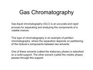
Chem 155 Unit 1 Page 9 of 3131.1.2 Chromatography – Chemical SeparationsDifferent chemicals flow through separationmedium (column or capillary) at different speeds‘plug’ of mixture goes in chemicals come out ofcolumn one-by-one (ideally)Gas Chromatography ‘GC’Powerful but Suitable for Volatile chemicals onlyLiquid Chromatography High Performance(pressure), ‘HPLC’ in it’s many forms –Electrophoresis -Liquids, pump with electriccurrent, capillary, gel, etc.Chromatogramabsorbancetime / sPage 9 of 313

Chem 155 Unit 1 Page 10 of 3131.1.3 Mass SpectrometryDetection method where sample is:volatilized,injected into vacuum chamber,ionized,usually fragmented,accelerated,ions are ‘weighed’ as M/z – mass charge.Often coupled to:chromatographlaser ablationatmospheric “sniffer”.Very sensitive (pg) quantitationPowerful identification toolPage 10 of 313

Chem 155 Unit 1 Page 11 of 3131.1.4 ElectrochemistrySimple, sensitive, limited to certain chemicalsIon selective electrodes (ISE’s):e.g. pH, pCl, pO 2 etc.ISE’s measure voltage across a selectivelypermeable membrane (e.g. glass for pH)E α log[concentration]ISE’s have incredible dynamic range!pH 4 pH 10[H+] = 0.0001 0.0000000001 MDynamic electrochemistry –measure current (i) resulting from redoxreactions at an driven by a controlled voltageat an electrode surfacei(E,t) α [concentration]1.1.5 GravimetryPrecipitate and weigh products –very precise, very limited1.1.6 Thermal AnalysisThermogravimetric Analysis TGAMass loss during heating – loss of waters ofhydration, or decomposition temperatureDifferential Scanning Calorimetry DSCHeat flow during heating or coolingPage 11 of 313

Chem 155 Unit 1 Page 12 of 3131.2 Instrumental vs. Classical Methods.SeparationClassicalMethods of Analytical Chemistry# ChemicalsIsolated / hrand amount(g)Extraction 1-2 gDistillation 1-2 gPrecipitation 1-2 gCrystallization 1-2 gInstrumentalHigh PerformanceLiquidChromatrographyGasChromatographyRelax, you don’t needto memorize this table– just humor Dr. Terrillwhile he talks about it.# ChemicalsIsolated / hrand amount(g)10 ng100 ngElectrophoresis 50 pgQualitativeSpeciationEstimated Number of uniquely identifiable molecules by methodCombination ofColor / SmellMelt / BoilingPoint,SolubilityWettingDensityHardness100’sUV-VisInfrared1,000’s100,000’sMass Spectrometry > 10 6NMRSpectroscopyBest Quantitative Precision and SensitivityTitration 0.1% 1 ppm> 10 6OpticalSpectroscopy 0.1% 10 -23 MQuantitationPrecisionGravimetry 0.01%1 ppmMassSpectrometry0.1%amount10 -4 %mass10 -13 MColorimetry10% 1 ppmNMRSpectroscopy 1%100pppmWhat are the more precise measurements that youhave made and what were they?Page 12 of 313

Chem 155 Unit 1 Page 13 of 3131.3 Vocabulary: Basic InstrumentalAnalyteThe chemical species that isbeing measured.MatrixThe liquid, solid or mixedmaterial in which the analytemust be determined.DetectorDevice that records physical orchemical quantity.Transducer The sensitive part of a detectorthat converts the chemical orphysical signal into an electricalsignal.SensorDevice that reversibly monitors aparticular chemical – e.g. pHelectrodeAnalog signal A transducer output such as avoltage, current or light intensity.Digital signal When an analog signal has beenconverted to a number, such‘3022’, it is referred to as a digitalsignal.Analog signals are susceptible to distortion, and soare usually converted into digital signals (numbers)promptly for storage, transmission or readout.Page 13 of 313

Chem 155 Unit 1 Page 14 of 3131.4 Vocabulary: Basic Statistics ReviewPrecisionRandom ErrorAccuracySystematic Error(bias)HistogramProbabilityDistributionIf repeated measurements of the same thing areall very close to one another, then ameasurement is precise. Note that precisemeasurements may not be accurate (see below).Random error is a measure of precision.Random differences between sequentialmeasurements reflect the random error.If a measurement of something is correct, i.e.close to the true value, then that measurement isaccurate.Systematic error is the difference between themean of a population of measurements and thetrue value.A graph of the number or frequency ofoccurences of a certain measurement versus themeasurement value.A theoretical curve of the probability of a certainmeasured value occurring versus the measuredvalue.A histogram of a set of data will often look like a Gaussian probability distribution.AverageThe sum of the measured .xvalues divided by the numbernnof measurements.MedianVariance (σ 2 )Standard Deviation(σ)Relative StandardDeviationPropagaion ofErrorx MEANHalf of the measurements fall above the medianvalue, and half fall below.A measurement ofprecision. The sum of thesquares of the randommeasurement errors.n 1A widely accepted‘standard’ measurement ofprecision. The square root nσof the variance.n 1The standard deviation divided by the mean, andoften expressed as : %RSD=σ/x MEAN 100%.σ 2 n x MEAN x n2When the mean of a set of measurement (x) hasa random error (σ x ), it is reported as x±σ x . If wewish to report the result of a calculation y=f(x)based on x, we propagate the error through thecalculation using a mathematical method.nx MEAN x n2Page 14 of 313

Chem 155 Unit 1 Page 15 of 3131.5 Statistics Review1.5.1 Precision and AccuracyHistogram of normally distributed events80MeanNumber of times it was observed604020Mean -onestandarddeviationMean +onestandarddeviation00 1 2 3 4 5 6Value observed1.5.2 Basic FormulaeHistogram of 1024 eventsMean : μlimN → ∞N∑ x NNPopulationStandardDeviation:σ xlimN → ∞x N − μ∑ ( )2NNAverage:x avg∑ x NNNSampleStandardDeviation:s xx N − x∑ ( avg )2NN−1Bias or absolute systematic error = x avg − μRelative standard deviation =sx avgPage 15 of 313

Chem 155 Unit 1 Page 16 of 313When you make real measurements of things you generally don’tknow the ‘true’ value of the thing that you are measuring. (Call thisthe true mean, μ, for now. For the purposes of this discussion let usassume that there is no systematic (accuracy) error (i.e. no bias).1.5.3 Confidence IntervalWHAT DO YOU DO TO ENSURE THAT YOUR ANSWER IS ASCLOSE AS POSSIBLE TO THE TRUTH?TAKE THE AVERAGEx AVGBut, you still don’t know the exact answer…SO WHAT DO YOU REALLY WANT TO SAY?I am highly confident that the true mean lies withinthis interval (e.g between 92 and 94 grams).In fact, there is only a 1 in 20 chance that I am wrong!How do you calculate what that interval is?You need to know:The average of the data set: xThe standard deviation: σ or sThe number of measurements (observations) made: NThis interval is called a confidence interval (CI). Which is better,abigger or a smaller CI?Smaller is better…How can you improve your CI?Make more measurements (N)Page 16 of 313

Chem 155 Unit 1 Page 17 of 313Confidence Interval (continued).If you know the standard deviation, σ, (less common case), then:The x% confidence interval for μ = x AVG ± zσ / N ½If you don’t know the standarddeviation, σ, (more commonly thecase), then:If you have only a roughestimate of x AVG , then you areless confident that it is close toμ, hence you divide by N ½ .The x% confidence interval for μ = x AVG ± ts / N ½In this case t is a function of NThis leaves only z and t – what are they? These numbers representthe multiple of one standard deviation (σ or s) that correspond to theconfidence interval. In the second case, s is only an estimate of σ, sothe error in s needs to be taken into account, so t is a function of the“number of degrees of freedom”. For our purposes, i.e. averagingmultiple identical measurements, the number of degrees of freedomis simply N-1.Page 17 of 313

Chem 155 Unit 1 Page 18 of 313An example:Assume that we do our best to measure the concentration of basicamines in a fish tank. Our answers are 4.2, 4.6, 4.0.N =3X AVG =(4.2+4.6+4.0) / 3 = 4.27s =(4.2-4.27) 2 +(4.6-4.27) 2 +(4.0-4.27) 23-1= 0.31Number of degrees of freedom for confidence interval =3-1=295% confidence limits for μ =5.45.04.27± (4.3*0.31) / (3 1/2 )= 4.27±0.93 or= 4.3 ± 0.9 or= 34to524.53.5Page 18 of 313

Chem 155 Unit 1 Page 19 of 3131.5.4 Confidence Interval (CI) in WordsConsider thisexperiment. You havea camera device thatmeasures thetemperature of objectsfrom a distance bymeasuring theirinfrared light emission.It is very convenientbut somewhat97.5, 96.0,99.197.32398.05599.051imprecise. Assume for the moment that the camera is perfectlyaccurate – that is, if you measure the same object with it many timesthe average temperature result will equal the true temperature.In order to evaluate the precision of your camera thermometer, youmeasure the temperature of each item three times. In each case youget an average and a standard deviation.PROBLEM 1: The average camera reading is sometimes higher thanthe true value, and sometimes lower, but you don’t know how toevaluate this fluctuation. In just a few words, how can youcharacterize this fluctuation?SOLUTION 1:Calculate the sample standard deviation.PROBLEM 2: A series of experiments, each of three measurementseach yields a set of sample standard deviations that also differenteach time! If you repeat the whole experiment, but this time youmeasure each sample ten times, then the standard deviations aremuch closer, but still not equal each time.Why does the sample standard deviation calculation give a differentresult each time? Assume for the moment that the cameraperformance (precision) is not changing.SOLUTION 2:Realize this fact: Sample standard deviations areonly estimates.Page 19 of 313

Chem 155 Unit 1 Page 21 of 313Use this table:% confidence interval°freedom 50 80 95 991 1.00 3.08 12.71 63.662 0.82 1.89 4.30 9.923 0.76 1.64 3.18 5.844 0.74 1.53 2.78 4.605 0.73 1.48 2.57 4.036 0.72 1.44 2.45 3.717 0.71 1.41 2.36 3.508 0.71 1.40 2.31 3.369 0.70 1.38 2.26 3.2510 0.70 1.37 2.23 3.1720 0.69 1.33 2.09 2.8550 0.68 1.30 2.01 2.68100 0.68 1.29 1.98 2.63Use this formula:CIμ± ⋅ts ⋅ NNote the following:For a straight average of Npoints, the number ofdegrees of freedom is N-1.Complete the following table:Passenger T AVG (°F) Stdev(°F)1 101.5 1.1Lowerboundaryof 80%CIUpperboundaryof 80%CIIs the probability thatthe passenger’sTemp is > 102°90% or more?2 98.57 0.173 103.93 0.047Page 21 of 313

Chem 155 Unit 1 Page 22 of 3131.5.6 t EXP PROBLEM:Another way of approaching this type of problem is to calculate anexperimental value of ‘t’ called t EXP.In the example below, we will compare a measured result with anexact one. The question one answers with t EXP is this: Am I confidentthat the observed value (x) differs from the expected value (μ)?Our threshold temperature, exactly 102° was tested, so we can makemeasurements and test the hypothesis that ‘the true temperature isgreater than 102°’.Given the following three measurements of a passenger’stemperature: 103.76°, 102.11°, 105.38° – calculate an experimentalvalue of the ‘t’ statistic for this population relative to the true value of102°. Average = 103.75, std dev = 1.34% confidence interval°freedom 50 80 95 991 1.00 3.08 12.71 63.662 0.82 1.89 4.30 9.923 0.76 1.64 3.18 5.84( x av − μ) ⋅ Nt expsμ = test value( 103.76−102) ⋅ 3t exp :=1.34t exp = 2.275Can you state with the given confidence that this person’stemperature differs from the expected value of 102°?99%? No95%? No80%? Yes50%? YesPage 22 of 313

Chem 155 Unit 1 Page 23 of 313C = analyte conc.m = slope calibration 1513.166Sb = signal for blankInstrument Signal (S)1.6 Calibration Curves and SensitivityCalibration Sensitvity:S = mC + S bS = instrument signalm = calibrationsensitivity10A highly sensitive instrument candiscriminate between small differences inanalyte concentration.ΔSΔC= mS ≈σ SiΔS5But, can wereallydistinguishΔCbetween smallchanges in0 00 20 40 60 80 100concentration?1000 C iAnalyte Concentration (C)γ = Analytical Sensitvityγ = m / σ Sγ = (ΔS/ΔC) / σ Sγ = 1/ΔC for the “ΔC”corresponding to σ Sm ≈andσ S ≈soγ ≈1 / γ = ‘noise’ inconcentration ≈σ C .So small γ is?GoodBadPage 23 of 313

Chem 155 Unit 1 Page 24 of 3131.7 Vocabulary: Properties of MeasurementsSensitivitySelectivitySpecimenSampleAnalyteCalibration CurveInterferantDetection Limit C MIN orC MLimit of Quantitation(LOQ)Limit of Linearity (LOL)Linear Dynamic Range(LDR)A detector or instrument that responds to only asmall change in analyte concentration issensitive. Numerically, the sensitivity of aninstrument is the slope of the calibration curve inuntis of: signal / unit concentration – often givenas ‘m’. Sometimes the detection limit (see below)is called the instrument sensitivity – but this is notcorrect.The ratio of the sensitivity of an instrument to ananalyte to that of an interferant.The material removed for analysis – e.g. a giventablet from an assembly line.The mixture that contains the chemical to bemeasured – e.g. the blood sample that we wantto measure iron in.The chemical that is being measured – e.g. theiron in the blood sample.A linear or non-linear function relating instrumentresponse (signal) to analyte concentration.Another chemical in the sample that either affectsthe instrument’s sensitivity to the sample or givesa signal of it’s own that may be indistinguishablefrom the analyte signal.The minimum detectable concentration ofanalyte. Usually defined as that concentrationthat gives a signal of magnitude equal to threetimes the standard deviation in the blank signal.The minimum concentration of analyte for whichan accurate determination of concentration canbe made. The LOQ is typically that concentrationfor which the signal is 10x the standard deviationof the blank signal.The largest concentration for which a calibrationcurve remains linear.The range of concentrations (or signal strengths)between the LOQ and the LOL. An instrument ismost useful within its’ LDR.Page 24 of 313

Chem 155 Unit 1 Page 25 of 3131.8 Detection LimitThe detection limit is denoted “C M ”C M is the minimum concentration that can be“detected,” or distinguished confidently from a blank.Let us define the minimum detectable signal changeas: ΔS MTherefore: ΔS M = mC M must be a multiple (n) of thenoise level in the blank: (σ b ).ΔS M ≡ 3σ b = mC MMinimumDetectable SignalSignal due toblankMinimumdetectableconcentrationBy convention, m=3.Derive a formula for C M based on σ B and m:mC M = 3σ bsoC M = 3σ b /mDerive a formula for C M based on γ :γ = m/σ so 1/γ = σ/mC M = 3σ/m = 3/γPage 25 of 313

Chem 155 Unit 1 Page 26 of 3131.8.1 A Graphical Look at Detection Limit (C MIN )Consider the minimum detectable signal in thecontext of the confidence interval:S MIN = 3σ b + S bTo what confidence interval does 3σ correspond?Assume N=2 (two replicate measurements of S b )zσ/N 1/2 = 3σ z/N 1/2 = 3 z = 3*1 1/2 = 3z = 3 corresponds to the 99.7% confidence intervalAnother way of saying this (crudely) is that weconsider a signal ‘detected’ when it falls outside of theboundaries corresponding to the 99.7% confidenceinterval for the blank signal.Page 26 of 313

Chem 155 Unit 1 Page 27 of 3131.8.2 Minimum Detectable Temperature Change?Using the thinking that we developed for the generalcase of signals with random error – what do you thinkis the probability that the following signal change isdue to random fluctuations?Page 27 of 313

Chem 155 Unit 1 Page 28 of 3131.8.3 Dynamic RangeLOQ = Limit of Quantitation (σ S /S ≈ 0.3)LOL = Limit of LinearityBetween LOQ and LOL your instrument is mostuseful!This is called:Linear Dynamic RangePage 28 of 313

Chem 155 Unit 1 Page 29 of 3131.8.4 SelectivitySometimes another chemical species will add to orsubtract from your analyte signal –S = m A C A + m B C B + m C C C + m D C D + … + S BAnalyte Interferants BlankSelectivity coefficients determine how serious aninterferant is to your determination of analyte C A :k B,A = m B /m A ,k C,A = m C /m A , etc…So:S = m A (C A + k B,A C B + k C,A C C + …) + S BPage 29 of 313

Chem 155 Unit 1 Page 30 of 3131.8.5 Direct InterferenceIn order to measure a concentration directly, withoutcorrections, k B,A , k C,A must be approximately:Zero!If there is interference, it is necessary to know both:k B,A , k C,AandC B , C Cbefore one can determine the desired quantity C A !Page 30 of 313

Chem 155 Unit 1 Page 31 of 3131.9 Linear RegressionLeast-SquaresRegression orLinear RegressionAssuming that a set of x,y data pairs are welldescribed by the linear function y = a+bx, andassuming that most error is in y (x is moreprecisely known) and the errors in y are not afunction of x, then the coefficients that minimizethe residual function:χ 2 = Σ(y I – (a + bx I )) 2can be found from the following equations:Non-linearRegressionStandard AdditionsPlotSample Matrix /Standards MatrixMatrix EffectInternal Standardsfrom Data Reduction and Error Analysis for thePhysical Sciences, Philip R. Bevington, cw. 1969Mc Graw Hill.Methods for fitting arbitrary curves to data sets.A nearly matrix-effect free form of analysis. Astandard additions plot is a linear plot ofinstrument signal versus quantity of a standardanalyte solution ‘spiked’ or added to the unknownanalyte sample. The unknown analyteconcentration is derived from the concentrationaxis-intercept of this plot.The matrix is the solution, including solvent(s)and all other solutes in which an analyte isdissolved or mixedA matrix effect refers to the case where theinstrumental sensitivity is different for the sampleand standards because of differences in thematrix.A calibration method in which fluctuation in theinstrument signals due to matrix effects are,ideally, cancelled out by monitoring thefluctuations in the instrument sensitivity tochemicals, internal standards, that are chemicallysimilar to the analyte.Page 31 of 313

Chem 155 Unit 1 Page 32 of 3131.9.1 Linear Least Squares CalibrationThe most common method for determining theconcentration of an unknown analyte is the simplecalibration curve.In the calibration curve method, one measures theinstrument signal for a range of analyteconcentrations (called standards) and develops anapproximate relationship (mathematically orgraphically) between some signal ‘S’ and analyteconcentration ‘C’.If the signal-concentration relationship is linear, then:S = S B + mC y = a + bxBut, one can not just draw the line between any twopoints because all the points have some error. So,one mathematically attempts to minimize theresiduals.χ 2 = Σ(y i – (a + bx i )) 21.51.5Instrument Signal (S)S iS iF i10.5F i10000 2 4 6 8 10Page 32 of 3130 C iAnalyte Concentration (C)

Chem 155 Unit 1 Page 33 of 313The values of a and b for which χ 2 is a minimum arethe following:The errors in the coefficients, σ a and σ b can be found,similarly, using:These quantities are best found using a computerprogram. Modern versions of Microsoft Excel willcalculate a and b for you (use ‘display equation’option on the ‘trend line’), and σ a and σ b if you havethe data analysis ‘toolpack’ option installed. Excel isalso fairly well suited to doing the sums and formulas.Page 33 of 313

Chem 155 Unit 1 Page 34 of 313See also, appendix a1C in Skoog, Holler and Nieman.But, be advised that there is a typo in older editions.Equation a1-32 should read:m = S XY /S XXAlso – it is a somewhat more subtle problem tocalculate the error in a concentration determined froma calibration curve of signal (y) versus concentration(x).You will need to follow Skoog appendix-a calculationsto deal with this problem in your lab reports whereyou determine an unknown concentration. M = thenumber of replicate analyses, N = the number of datapoints.Equation a1-37Skoog 5th edition.s cs y⋅m1M+1N+( ) 2yc avg− y avbm 2 ⋅S xxNote: when computing a confidence interval using thiss C value, the degrees of freedom are N-2. (See forexample Salter C., “Error Analysis Using theVariance-Covariance Matrix” J. Chem. Ed. 2000, 77,1239.Page 34 of 313

Chem 155 Unit 1 Page 35 of 3131.10 Experimental Design:Designing an experiment involves planning how youwill: make calibration and validation standards;prepare the sample for analysis; and perform themeasurements.1.10.1 Making a set of calibration standards.1. You need to know the dynamic range of yourinstrument.2. You need to know the sample sizerequirement of your instrument.3. You need to know the estimated expectedconcentration of your sample.4. You need to prepare and dilute your sampleuntil it is a. within the dynamic range of yourinstrument and b. such that there is enoughsolution to measure.5. You need to choose target standardconcentrations that bracket the expectedsample concentration generously – e.g. by afactor of 2 to 3. For example, if your expectedconcentration is 5.3 ppm, you may wish to makea calibration set that consists of standards thatare about 2,4,8,10 and 12 ppm.Page 35 of 313

Chem 155 Unit 1 Page 36 of 3136. You need to make a primary stock solution,the concentration of which you know accuratelyand precisely. This solution will usually bemore than twice as concentrated as your mostconcentrated calibration standard. You willdilute this primary stock solution to make thecalibration standards. You need to have enoughto make all of your calibration standards.7. You need to choose the pipets and volumetricflasks that you will use to perform the dilutions.This means that you plan the preparation ofeach standard. This takes some planning andcompromising and many choices – there aremany ways to do this correctly – there is morethan one right answer!8. Decide on and record a labeling system inyour notebook, collect the glassware, and dothe work. I have a labeling system for yourcaffeine, benzoic acid, iron and zinc standards –I need you to use these labels so that we cansort things out in the class.Page 36 of 313

Chem 155 Unit 1 Page 37 of 3131.10.2 Exercise in planning an analysis:Assume that you will be analyzing sucrose in cornsyrup sweetened ketchup packets. The packets arethought (i.e. expected) to contain about 0.8 grams ofcorn syrup that is about 70% sucrose by weight. TheHPLC instrument that you will be using can detectsucrose by refractive index in the 0.1-20 parts perthousand (ppth) range (this is the instrument’sdynamic range for sucrose). You have pure sucrosefor standards, and will be making five calibrationstandard solutions. The instrument requires between250 and 1000 μL of sample.You have the following glassware at your disposal:PipetsVolumetric FlasksVolume RelativePrecisionVolume RelativePrecision20-200 μL 5-1% 1 mL 1%1 mL 1% 5 mL 1%5 mL 1% 10 mL 1%10 mL 1% 25 mL 1%15 mL 1% 50 mL 1%20 mL 1% 100 mL 0.5%25 mL 0.5% 250 mL 0.5%50 mL 0.5% 1000 mL 0.25%Page 37 of 313

Chem 155 Unit 1 Page 38 of 3131.10.3 Plan the analysis!1. If you dissolve the packet in water, dilute it to100.0 mL and filter it, what will the approximatesucrose concentration be (ppth)?0.8 gsyrup0.7 gsucrose 1100 mLg syrup water1000 mgsucroseg sucrose1 mLwater1 gwater= 5.6 ppthIs this within the dynamic range?Would it be better to use 10, 25 or 50 mL ofwater?2. You need to prepare a stock solution of sucroseto make the calibration standards. Whatconcentration should this stock solution be?1, 10, 100 or 1000 ppth?3. How much sucrose would be required to make:1, 10, 100 or 1000 mL of this solution?1.0mL100 mgsucrose =1 mLsoution100 mgsucrose =0.100 gsucrose10 mL =>1.00 gsucrose100mL =>10.0 gsucrosePage 38 of 313

Chem 155 Unit 1 Page 39 of 3131.10.4 How to make primary stock solution:1. Weigh out the desired quantity of pure (e.g. dry,or oxide-free) analyte material.2. Dissolve this amount quantitatively, i.e. withoutany loss, in the desired solvent.3. Transfer this liquid quantitatively into thedesired volumetric flask.4. Dilute to volume with the desired solvent – thisprocess is important! It is often poor practice toadd 5 mL of ‘a’ to 5 mL of ‘b’ and anticipate thatthe final volume will be exactly 10 mL!Remember the words DILUTE TO VOLUME!Page 39 of 313

Chem 155 Unit 1 Page 40 of 3134. What concentrations ‘bracket’ the 5.6 ppthtarget?For example:5.2, 5.4, 5.6, 5.8, 6.0 ppth--- or ---1, 2, 4, 6, 8 ppth--- or ---1, 2, 5, 10, 15 ppth--- or ---0.050, 0.50, 5.0, 50, 500 ppthDo you need to makestandards on an evenspacing?No – but calibrationpoints above andbelow the std. areneeded.Does the analytehave to fall right in themiddle of thecalibration standards?No, but itminimizeserror!5. What volumes of standards should you prepare?How much is needed by the instrument?What is the smallest volume that you canconveniently and precisely measure?How expensive is the analyte and solvent?How expensive is it to dispose of the waste?0.1 or 1 or 10 or 100 or 1000 mLPage 40 of 313

Chem 155 Unit 1 Page 41 of 3136. How do you prepare the calibration series fromthe primary stock solution?Primary Stock (1) is diluted to make Calibration Standard (2)C 1 V 1 = C 2 V 2First calibration standard:10 mL of 1 ppth sucrose from 100 ppth stocksolution.C 1 = 100 ppthC 2 = 1 ppthV 2 = 10.0 mLV 1 = ? = volume to pipet overV 1 = C 2 V 2 /C 1Page 41 of 313

Chem 155 Unit 1 Page 42 of 3137. How to plan a set of standard preparations in theMS Excel spreadsheet program:Calibration Standard Preparation:Target Conc: Stock Conc: Final Volume: Volume to Pipet:C2 / ppt C1 / ppt V2 / mL V1=C2*V2/C11.00 100.0 10.00 0.100 mL2.00 100.0 10.00 0.200 mL5.00 100.0 10.00 0.500 mL10.00 100.0 10.00 1.000 mL15.00 100.0 10.00 1.500 mLCalibration StandTarget Conc: Stock Conc: Final Volume: Volume to Pipet:C2 / ppt C1 / ppt V2 / mL V1=C2*V2/C11 100 10 =A4*C4/B4 mL2 100 10 =A5*C5/B5 mL5 100 10 =A6*C6/B6 mL10 100 10 =A7*C7/B7 mL15 100 10 =A8*C8/B8 mLThese are formulas that you type intoExcel – normally only the result of theformula calculation is displayed.Page 42 of 313

Chem 155 Unit 1 Page 43 of 3131.11 Validation – Assurance of Accuracy:Calibration and linear regression optimizes theprecision of a calibration curve determination but acalibration curve can only be said to be accurate if:the analysis has been validatedAnother way of saying this is that a method is valid if:all significant sources of biashave been removedValidation addresses the various aspects of ananalysis that can ‘go wrong’ and give you a wronganswer.The table below lists some of the aspects of ananalysis that can be invalid, and suggests ways tovalidate them.Source of bias:Analyst erraticError in analysttechniqueCalibrationstandards are inerror (are not whatthey say the are)CalibrationmethodInstrumentfunction erraticInstrument driftPossible Solution(s):Analyst can repeat experimentDifferent analyst does same analysis andgets same result.Entire analysis Independent standardrepeated with measured periodically -indpendent called validation standardcalibration or QC standard (qualitystandard set control)Different calibration method used (standardadditions)Different instrument used (can be a differentkind of instrument)Periodically measure validation standard orinternal standardPage 43 of 313

Chem 155 Unit 1 Page 44 of 313In general validation of an analysis is done usingsome kind of independent analysis of the sample.• For the purposes of this class, if the two methodsagree (t-test does not show a difference) then themethod is said to be validated.• If the two methods disagree (i.e. there isevidence of bias), then there is evidence forsystematic error like a matrix effect, aninterferant, or a mistake in the preparation ofstandards or samples.If an analysis is repeated as described below, whataspects of the analysis are validated (i.e. what musthave been ‘good’ for the answers to have come outthe same)?Validation ApproachCompletely independentmeasurements of thesame sample using adifferent instrument ortechnique.Use the same method,but measureindependently preparedstandards as samples.Aspect(s) validatedCalibration method,including matrix effects.Instrument, includingdistortion and drift.You! The analyst, did itrightYou! The analyst made nomistakes in theimplementation of theprocedure.Page 44 of 313

Chem 155 Unit 1 Page 45 of 3131.12 Spike Recovery Validates Sample Prep.To do a spike recovery analysis, one takes replicatesamples and to a subset of them adds a spike ofanalyte before the sample prep begins. So, forexample, one could take four vitamin tablets, anddivide them into two groups of two. To one group onecould add some Fe, say half the amount originallyexpected. For example, if there is supposed to be 15mg of iron in the tablet, one could spike two sampleseach with 5 mg of iron and leave two unspiked.Acids etc.digestfilterDilute to100 mLvolumeAnalyze 140ppm14.0 mgfoundSampleSample+ 5.00mg spikedigestfilterDilute to100 mLvolumeAnalyze 187ppm18.7 mgfound18.7-14.0 = 4.7 mg of spike found: spikerecovery percent = 4.7 / 5.00 94%What does this say aboutour sample preparationmethod?We may be losing about6% of the analyte duringsample prep.Page 45 of 313

Chem 155 Unit 1 Page 46 of 3131.13 Reagent Blanks for High Accuracy:A reagent blank is a blank that is made by doingeverything for the sample prep etc. but without thesample:Acids etc usedin sample prep.digestfilterDilute to100 mLvolumeAnalyze 2.3ppm0.23 mgFe found“No Sample” sample.Ultrapurewater blankIn this example the reagent blank is analyzed againstultrapure water. The 0.23 mg Fe found in the reagentblank may be due to Fe impurities in the acids, but italso may be a matrix effect. In either case, itsuggests that we should do what in order to arrive ata more accurate result?Either:a. analyze all standards and samplesagainst reagent blanks orb. subtract the signal from the reagentblank against result from sample resultsmade with pure water blanks!Page 46 of 313

Chem 155 Unit 1 Page 47 of 3131.14 Standard additions fix matrix effects:Use the method of standard additions when matrixeffects degrade the accuracy of the calibration curves.There is one important assumption built into thecalibration curve idea. That assumption is thefollowing:the sensitivity of the instrument to the analyte in the standards isEQUAL TOthe sensitivity of the instrument to the analyte in the sample matrixWhy would the sensitivity be different?1. Many Instruments are sensitive to things like:1. pH 2. ionic strength 3.organiccomponents of the solvent matrix2. Sometimes other chemicals can change thecalibration sensitivity by:chemically binding to or interacting with theanalyte atom/moleculeThese two things are examples of:Matrix EffectsPage 47 of 313

Chem 155 Unit 1 Page 48 of 3131.14.1 How does one deal with matrix effects?1. Make the sample and standard matrix as nearlyidentical as possible:matrix matchingBut – matrix matching requires that you already knowa lot about your ‘unknown’ – often not the case. So,the matrix-immune alternative to the calibration curveis to:2. Use the method of: standard additions:In other words, the assumption built into thecalibration curve method is that the matrix effects arenegligible or identical for standards and samples. Ifthis can not be assumed, one must match the sampleand standard matrices.The way that the method of standards additions doeswith this is to dilute both standards and samples:in the same matrix (solution)Page 48 of 313

Chem 155 Unit 1 Page 49 of 3131.14.2 An Example of Standard Additions:1. The analyte sample is split up into e.g. 6 aliquots ofidentical, known volume – e.g. 1.00 ml.2. To each of these, a known quantity of standard(known as a spike) is added – e.g.0, 0.1, 0.2, 0.3, 0.4, 0.5 ml – standard is dissolvedin known matrix like water or 0.1M pH 7 phosphateetc.3. Each aliquot is diluted to a total volume.1. Add sample2. Add standard3. Dilute to volume,and mix mix mix!Note: you split and diluteyour sample – how doesthis impact the precision ofyour measurement?How does this processimpact the accuracy ofyour measurement?Page 49 of 313It decreases it!If volume change is big.It increases it!

Chem 155 Unit 1 Page 50 of 3131.14.3 Calculating Conc. w/ Standard Additions:a'ab'bOne way of analyzing this uses similar triangles:a / b =a’/b’The y-axis absorbance signal (S) is proportional to the moles ofanalyte (V X C X ) and standard (V S C S ).The x-axis is simply the standard ‘spike’ volume.The x-intercept is the hypothetical spike volume (V S ) 0 containing thesame amount of analyte as the sample.a is proportional to moles of analyte in the sample = V X C Xa’ is proportional to moles of std added = V S C Sb is (V S ) 0 – the x-intercept of the graphb’ is V S – the spike volumeSubstitute for a,a’,b,b’:V X C X(V S ) 0=V S C SV SSolve for C X :C X = C S (V S ) 0 /V XPage 50 of 313

Chem 155 Unit 1 Page 51 of 3131.14.4 Standard Additions by Linear Regression:Let:V X = volume of unknown analyte solution added to each flaskC X = concentration of unknown solutionV T = final, diluted volumeV S = volume of ‘spike’ added to unknown soln. before dilutionC S = concentration of analyte in spike solutionDilution Calc 1: (V 1 C 1 = V T C T C T = V 1 C 1 /V T )Contribution to concentration of analyte from sample:V X C X /V TDilution Calc 2:Contribution to concentration of analyte from spike:V S C S /V TTotal Signal (sensitivity = k) given that ‘x’ variable is C S .S = kV X C X /V T+ kV S C S /V TSlope = m =kC S /V Tintercept = b =kV X C X /V Twe can get b and m from linear regressionand we want C X … so … b/m = =so : C X =bC SmV XkV X C X /V TkC S /V TV X C X /C SPage 51 of 313

Chem 155 Unit 1 Page 52 of 3131.15 Internal StandardsInternal standards can correct for sampling, injection, optical pathlength and other instrument sensitivity variations.An internal standard is a substance added (or simply present) inconstant concentration in all samples, and standards.When something unexpected decreases the sensitivity of theinstrument (m) so the signal drops (S = mC + S B ) – it can beimpossible to distinguish this from a change in analyte concentrationwithout an internal standard.Consider the ratio of the blank corrected analyte ( S'S'ANmANCANCinternal standard (IS) signals (S): = = kS'm C CISISISANANIS= SAN− sB) to theAssumes for the moment that k is a constant, i.e. invariant to factorsaffecting overall instrumental sensitivity. As an example, let’sconsider k to be a correction for injection volume in achromatographic system. It is perfectly reasonable to assume that anaccidentally low or high injection volume would affect the internalstandard and analyte signals identically – e.g. if a given injection were6% high, then both analyte and internal standard peaks would be 6%larger than expected.If k is invariant to instrument fluctuations, then the true analyteconcentration can always be derived from the ratio of the correctedsignals so long as the internal standard concentration remainsconstant.Anlalyte conc. in a sample.S CC = 'AN ISANS'ISkwhere C ISis easily derived from a previously measuredkcalibration standard for which the analyte signal ( S'A − STD) andconcentration ( CA − STD) of the analyte and internal standardS'A−STDCIS−STDmAN( S'IS− STD, CIS−STD) are known: k ==S'C mIS−STDA−STDISPage 52 of 313From a calibration standard.

Chem 155 Unit 1 Page 53 of 313In other words, if C IS is held constant in all experiments, then theratio of the analyte to internal standard signals will beindependent of instrument sensitivity.When to use an internal standard?When substantial influence on instrument sensitivity is expected dueto variation in things like:Sample matrixTemperatureDetector sensitivityInjection volumeAmplifier (electronics) drift Flow rateAn internal standard must:a. not interfere with your analyteb. ideally have the same dependence on the chemical matrix,temperature (or other troublesome variable) as the analyte.Consider the ubiquitous ‘salt plate’ IR sampling method. A drop ofanalyte is sandwiched between two salt plates and this is placed inthe IR beam. The path-length is highly variable from experiment toexperiment. The signal A = εbC where ε is characteristic of themolecule, b is pathlength and C is concentration. If you are doing anexperiment to measure the increase in amide formation versus timeby the intensity of the amide bands near 1700 cm -1 . You could takesamples and measure them periodically, but the variability of thepathlength would distort the results.On the other hand, if all the samples were spiked with the sameamount of acetonitrile then the sharp nitrile stretch at 2250 cm -1 couldbe used as an internal standard.Page 53 of 313

Chem 155 Unit 1 Page 54 of 3131.15.1 Internal Standards Example:In HPLC the sample is injected into a flowing stream, and the signalis a peak in a plot of absorbance versus time (a chromatogram).Often the volume of the injection will vary from injection to injection,so the peaks will vary in size!Peak 1 is theinternal standard.100 ppm NaNO 3 ,480 All mAu . sabsorbance10.5Peaks 2, 3 and 4 are otheringredients in the sample.1Peak 5 is theanalyte, a caffeinestandard, 25 ppm,530 mAu . sabsorbance100 ppm NaNO 3 ,520 mAu . sabsorbance00 400 800 1200 1600 2000 2400 2800 3200 3600 4000time / s10.500 400 800 1200 1600 2000 2400 2800 3200 3600 4000time / s10.523Chromatogram1 is a standard.Did the caffeineconcentrationincrease fromchromatogram1 to 2?Did the caffeineconcentrationincrease inchromatogram1 to 3?Unknowncaffeine conc.630 mAu . s00 400 800 1200 1600 2000 2400 2800 3200 3600 4000time / sPage 54 of 313

Chem 155 Unit 1 Page 55 of 3131.15.2 Internal Standards CalculationHow about calculating the actual concentration of the sample in 3above?StandardS'A − STDCA − STDS'IS − STDCIS− STD530 mAu . s25 ppm480 mAu . s100 ppmSCA−STDIS−STDk ==S'IS−STDCA−STDS'ANmm' 530⋅100ANIS480⋅25= 4.417 unitless630 mAu . sSampleS'ISCISCANS'S'ISCk520 mAu . s100 ppmAN IS=630⋅100520⋅4.417= 27.4 ppmPage 55 of 313

Chem 155 Unit 2 Page 56 of 3132 Propagation of ErrorSkoog Chapters Covered:Appendix a1B-4 a1B-5 and – eqn. a1-28 table a1-5There is a general problem in experimental science and engineering:How to estimate the error in calculated results that are based onmeasurements that have error?Let’s consider the sum of two measurements a and b that both havesome fluctuation s a = 0.5 lb and s b = 0.5 lb.Let’s also pretend that we know the true values of a and b.True value of:a = 5.0 lbb = 5.0 lbLet’s say that we are weighing a and b and putting them into a box forshipment. We need to know the total weight. Our scale is really bad(poor precision, lots of fluctuation), and it can’t weigh both a and b atthe same time because it has a limited capacity. So, we have to firstweigh a, then b and then calculate the total weight. But we know thatthere is a problem with fluctuations, so we repeatedly weigh the sameitems a and b and do the following experiment:Characteristics of numbers insum ‘a’ and ‘b’Characteristics of sum‘c’Trial # Weight of: Deviation: Total DeviationA b da db weight: from avg:1 4.5 4.5 -0.5 -0.5 9.0 -12 5.5 4.5 +0.5 -0.5 10.0 03 4.5 5.5 -0.5 +0.5 10.0 04 5.5 5.5 +0.5 +0.5 11.0 +1average 5.0 5.0 0.5 0.5 10 0.5This is somewhat artificial and is not quite right, but it gives you thegeneral idea. Errors in a and b propagate into c.Page 56 of 313

Chem 155 Unit 2 Page 57 of 313From this example above, one would conclude that the fluctuation inthe sum is equal to the fluctuation in the numbers summed – but thisis not right.Which is bigger?a. the fluctuations in the individual numbers summedb. the fluctuations in the sumGraphically we consider here a similar case, for clarity we let a havea slightly larger fluctuation than b.a = 5 ± 2, b = 3± 1a+sa+b+sbtheoreticala+sa+b-sba-sa+b-sbcaa+saa-saa-sa+b+sb“Real”distributiontheoreticalPage 57 of 313

Chem 155 Unit 2 Page 58 of 313error propagation through sums:a := rnorm( 10000, 3,0.5)b := rnorm( 10000, 3,0.5)c:=a + b00002.78103.55406.334a=122.662.763b=123.3311.98c=125.9914.74432.52433.48236.00642.15743.84846.005mean( a) = 3.004stdev ( a) = 0.498mean( b) = 2.996stdev ( b) = 0.504mean( c) = 6stdev ( c) = 0.712a_distb_distc_dist:=:=:=histogram( 40,a)histogram( 40,b)histogram( 40,c)0.5 2 + 0.5 2 = 0.7071000a_dist j,1b_dist j,1500c_dist j 1,a dist j 0 b dist j 000 2 4 6 8 10, , c dist j 0Page 58 of 313

Chem 155 Unit 2 Page 59 of 313error propagation through products:c =c := i0123456789101112131415a ⋅b i i09.8818.8615.4738.7898.3018.0577.5619.9093.5897.4719.2066.0541.9440.6435.7738.27mean( c) = 9.003stdev ( c) = 2.156a_dist :=b_dist :=c_dist :=a_dist j,1b_dist j,1histogram( 40,a)histogram( 40,b)histogram( 40,c)1000500c_dist j, 100 5 10 15 20 25a_dist j, 0 , b_dist j,0 , c_dist j,0Page 59 of 313

Chem 155 Unit 2 Page 60 of 313For a simple example – if you construct a simple calibration curve ofinstrument signal versus concentration, and then use a real (i.e.noisy) signal to determine concentration.Errors propagate from S to C according to the sensitivity.Page 60 of 313

Chem 155 Unit 2 Page 61 of 313Let’s consider an example wherein the relationship between themeasured signal and the desired quantity is non-linear :AbsorbanceA = -log (P/Po)Absorbance is a nonlinear function oflight power - the measured quantity in aspectrophotometric experiment.Alog P P l21.5A i10.500 0.1 0.2 0.3 0.4 0.5 0.6 0.7 0.8 0.9 1P iObviously – the same error in P can give rise to different errors in A!This is a propagation of error problem. How can you calculate theerror in A that should result from a particular error in P?Page 61 of 313

Chem 155 Unit 2 Page 62 of 313Obviously, the answer has to do with the way that the dependentvariable (A) in this case changes as a function of the independentvariable (P).Consider a calculated value ‘S’ that depends on the measuredquantites, e.g. instrument signals, a,b,c…S = f(a,b,c…)In fact – the variance in S is proportional to the variance in a,b,c –and the proportionality is the partial derivative squared:(Skoog appendix a1B-4 has a derivation if you are curious)for: S f( a±σ a , b±σ b , c±σ c )σ S2⎛⎜⎝δSδa⎞ ⎟⎠2⋅σ a2+⎛⎜⎝δSδb⎞ ⎟⎠2⋅σ b2+⎛⎜⎝δSδc⎞ ⎟⎠2⋅σ c2So – let’s take an example:S = a+b-cfind σ S = f(S,a,σ a , b,σ b ,c,σ c )Note that the larger terms dominate!Page 62 of 313

Chem 155 Unit 2 Page 63 of 313Exercise: Prove the “multiplication / division rule”Show that for S = a*b/cσ S2S 2 σ a2a 2 σ b22σ cb 2 c 2Page 63 of 313

Chem 155 Unit 2 Page 64 of 313The propagation of error rules for special cases:Page 64 of 313