Mixture Design Tutorials - Statease.info

Section 7 – Mixture Design
Tutorials
Mixture Design and Analysis
Rev. 5/10/02
This tutorial shows how you can use Design-Expert ® software for mixture experiments.
A case study provides a real-life feel to the exercise. Due to the specific nature of the
case study, a number of features that could be helpful to you on mixtures will not be
exercised in this tutorial. Many of these features are used in the Factorial and Response
Surface tutorials, so you will benefit by doing them also.
We presume that you can handle the statistical aspects of mixture designs. If you need
further background, look in the Help system of Design-Expert. To learn all the tricks,
attend our Mixture Design For Optimal Formulation workshop. Call Stat-Ease for a
schedule or visit our web site (www.statease.com).
This tutorial provides only the essential program functions. For more details, check out
the Help system, which you can access at any time by pressing F1. Its hypertext search
capability makes it easy for you to track down the information you need.
The formulators measured two responses in a detergent formulation:
• Y1 - viscosity
• Y2 - turbidity.
while varying three components as shown:
• 3% ≤ A (water) ≤ 8%
• 2% ≤ B (alcohol) ≤ 4%
• 2% ≤ C (urea) ≤ 4%
They required that these three active components always equal nine weight-percent of
the total formulation, that is, A + B + C = 9%. The other components (held constant)
then must equal 91 weight-percent of the detergent.
The experimenters chose a standard mixture design called a simplex-lattice. They
augmented this design with axial check blends and the overall centroid. The vertices
and overall centroid were replicated, which increased the size of the experiment to a total
of 14 blends.
Design-Expert 6 User’s Guide Mixture Design Tutorials • 7-1

Design the Experiment
This case study leads you through all the steps of design and analysis for mixtures.
Follow up with the next tutorial to see how you can simultaneously optimize the two
responses.
Start the program by finding and double clicking on the Design-Expert icon. The menu
bar will display at the top of the program window. Take the quickest route to initiating a
new design by clicking on the blank-sheet icon � on the left of the toolbar. The other
route is via File, New Design (or associated Alt keys).
Main Menu and Tool Bar
Click on the Mixture tab. Design-Expert offers extensive choices for your design.
Detailed information on these can be found in the Help system.
Simplex Lattice Design
In this case, the formulator wants to use the default mixture design: the simplex-lattice,
but for 3 components, not 2. Click on the Mix Components pull down list and select
3. Enter the component and constraint information as shown below in the Name, Low
7-2 • Mixture Design Tutorials Design-Expert 6 User’s Guide

Rev. 5/10/02
and High fields, pressing the Tab key after each entry. Then enter 9 in the Total field
and % in the Units field.
Upon completing your data entry, your screen should look like the following screen.
Mixture Components - Entered Values
Continue with the process by pressing the Continue button at the lower right of the
screen. Immediately a warning appears.
Warning of Adjustment
Press OK. Notice that, although you entered the high limit for water as 8%, Design-
Expert adjusts it to 5%.
Mixture Components - Adjusted Values
It must do this because of the constraints:
1. All components must add to 9%.
2. Alcohol must be at least 2%.
3. Urea must be at least 2%.
That leaves 5% maximum of water (9 – 2 – 2 = 5) in any one experimental run. An
alternative way to adjust constraints would be to keep the upper limit of water at 8% and
then reduce the lower limits of the other two components to 0.5% each. Then the total
would meet the 9% goal. Design-Expert adjusts the upper constraint, but you can
override this by making your own adjustments. If you ask for unattainable lower limits
Design-Expert 6 User’s Guide Mixture Design Tutorials • 7-3

of your mixture components, the program will adjust the lower limit. In any case,
Design-Expert will help you build rational constraints.
Click on Continue to further specify the design.
Now you must choose the order of the model that you expect to be appropriate for the
system being studied. By default, Design-Expert uses Scheffe polynomials as mixture
models. In this case, you can assume that a quadratic polynomial, which includes
second order terms for curvature, will adequately model the responses. Leave the
default at Quadratic.
Simplex-Lattice Design Form
Via the following fields, Design-Expert provides options to strengthen the core simplex
design:
• “Augment design,” checked (�) by default, adds the overall centroid and
axial check blends to the design points.
• “Number of runs to replicate,” defaulted to 4, causes the specified number of
highest leverage experiments to be duplicated.
Accept these defaults by pressing Continue to the next step in the design process.
For Responses, select 2. Then enter the response Names and Units as shown
below.
Response Names and Units
You can step Back through the design forms and change what you want anywhere along
the way. When you press Continue on this page, Design-Expert will complete the
design setup for you.
7-4 • Mixture Design Tutorials Design-Expert 6 User’s Guide

Save the Data to a File
Rev. 5/10/02
Your standard (“Std”) order will most likely be different from the one we show below.
The software re-randomizes the run order each time a design is created. Always save
your design to disk to preserve a particular run order.
Completed Mixture Design - Run Order (Your run order may differ)
Now that you’ve invested some time into your design, it would be prudent to save your
work. Click on File menu item and select Save A s.
Save As Selection
The program displays a standard file dialog box. Use it to specify the name and
destination of your data file. Enter a file name in the field with the default extension of
dx6. (We suggest tut-mix). Then click on Save.
The three columns on the left of the design layout identify the experimental runs in
different ways – by standard order, by run order and by block number. Do a right click
with the mouse at the top of the column labeled Std. Then select Sort by Standard
Order.
Design-Expert 6 User’s Guide Mixture Design Tutorials • 7-5

Sorting by Standard Order
Components in Coded Values
It’s convenient to put the design in a coded format so calculations remain unaffected by
units of measure. You may be familiar with the coding used for factorial design, where -
1 designates the lowest level and +1 the highest level of each factor. Mixtures get
treated a bit differently, with a coding of 0 for lowest concentration and 1 for the highest
concentration. These coded values are called “Pseudocomponents.” They are calculated
from an intermediate stage called “real values.” Check these out by selecting Display
Options, Mixture Components, Real.
Components in Real Values
Real components are defined as:
Real = Actual / ( Total of Actuals)
Ri = Ai ∑A
/
For the first experiment in standard order:
R1 = 5/9 = 0.556
R2 = 2/9 = 0.222
R3 = 2/9 = 0.222
i
7-6 • Mixture Design Tutorials Design-Expert 6 User’s Guide

Edit the Design
Notice that the real values always sum to 1.0.
To look at the design in pseudo values, select Display Options, Mixture
Components, Pseudo.
Components in Pseudo Values
Pseudocomponents are defined as:
Pseudo = (Real − Li) / (1 − L) where
For the first experiment:
Li = lower constraint in real value
L =sum of lower constraints in real value
Pi = (Ri – Li) / (1 – L)
P1 = (0.556 – 0.333)/(1 – 0.777) = 1
P2 = (0.222 – 0.222)/(1 – 0.777) = 0
P3 = (0.222 – 0.222)/(1 – 0.777) = 0
Rev. 5/10/02
The value of one for P1 indicates that blend number one in standard order will be at the
richest possible level for water: 5%.
Now you will edit the design. In design selection you chose a simplex-lattice design to
fit a quadratic model. The design was augmented with the overall centroid and the axial
check blends. You asked that four experiments be replicated. Design-Expert chose the
four with the highest leverages: the three vertices and one edge. Assume that the
formulator wants to duplicate the overall centroid rather than the one edge. You can do
this in the design layout.
First, right click on the top of the Std column (the header) and Display Design ID,
then right click again and choose Sort by Design ID. The “ID” identifies unique
combinations and thus reveals duplicates explicitly. Now right click on the Block
column header and choose Display Point Type. This identifies the points and makes
it easier to find the ones you need. Look for the edge point that has been duplicated. It
will be a binary blend of two of the components, each with a pseudo value of 0.5, and
the remaining component with a pseudo value of 0. Click on the button just to the left of
Design-Expert 6 User’s Guide Mixture Design Tutorials • 7-7

the duplicated row to select it. Then eliminate it by right clicking on the row button
and selecting Delete Row(s).
Deleting a Duplicate Row (your duplicate may be a different edge point than shown)
Click Yes when prompted. Now locate the overall centroid, which is the row with equal
amounts of each factor: 0.333 in pseudocomponent coding. Click on the button just to
the left of the row. Then right click on the row button and select Duplicate.
Duplicating an Experiment
You can also add points by right clicking on the row button and selecting Insert Row.
You can edit component and response names by right clicking on the response column
heading and selecting Edit Info. Run or block numbers can also be changed.
Finally, since the design runs are changed, you should assign a new random run order.
Right click on the Run column heading and select Randomize. Then click on OK for
the default of All blocks.
Randomize Run Order Dialog Box
Having changed your experiment design, you should now save the changes. First put it
back into the form you will need to actually run the experiment: Select Display
7-8 • Mixture Design Tutorials Design-Expert 6 User’s Guide

Analyze the Results
Rev. 5/10/02
Options, Mixture Components, Actual and View, Run Order. Then select File,
Save to store the changes in your current file.
Assume that the experiments are now complete. You now need to enter the responses
into the Design-Expert software. For tutorial purposes, we see no benefit to making you
type all the numbers. Therefore, to save time, read the response data in from a file that
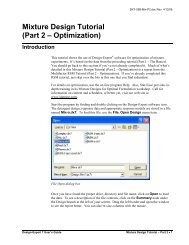
we’ve put on your program disk. Select File, Open Design. Click on the file called
Mix.dx6. Then press OK. You now should see response data (no need to type it in!).
Before moving on to the analysis, do a right mouse click on the top of the Block
column and select Display Point Type.
Showing Point Type on Filled-in Run Sheet (from file that comes with program)
Again do a right click on what is now labeled as the Type column. This time select
Sort by Point Type. You now get a very useful layout of the design.
Mixture Design Sorted by Point Type
Design-Expert 6 User’s Guide Mixture Design Tutorials • 7-9

The next step in the process is to analyze the data. Begin the analysis phase by clicking
on the node for Viscosity (to left of window).
First Step in the Analysis: Transformation Dialog Box
You now will work across the buttons at the top of the window. First, consider doing a
transformation on the response. In some cases this will improve the statistical properties
of the analysis. For example, when responses vary over several orders of magnitude, the
log scale usually works best. For this data, leave the selection at its default, None,
because no transformation will be needed.
Click on the Fit Summary button next. At this point Design-Expert fits linear,
quadratic, special cubic and full cubic polynomials to the response.
Fit Summary Table: Sequential Model Sum of Squares
7-10 • Mixture Design Tutorials Design-Expert 6 User’s Guide

Rev. 5/10/02
You may need to widen your window to get the entire output showing. Just move the
cursor to the left edge until it changes to a double-ended arrow. Then drag it open. In
similar fashion, you can also adjust column widths in any table or report. This may be
necessary to uncover the entire text. To move around the display, use the side and/or
bottom scroll bars, if necessary.
First, look for any warnings about aliasing. In this case, the full cubic model could not
be estimated by the chosen design - an augmented simplex design. Remember that you
chose only to fit a quadratic model, so this should be no surprise.
Next, you see the “Sequential Model Sum of Squares” table. The analysis proceeds
from a basis of the mean response. This is the default model if none of the factors cause
a significant effect on response. The output then shows the significance of each set of
additional terms:
• “Linear”: the significance of adding the linear terms after accounting for the
mean. (Due to the constraint that the three components must sum to a fixed
total, you will see only two degrees of freedom associated with the linear
mixture model.)
• “Quadratic”: the significance of adding the quadratic terms to the linear
terms already in the model.
• “Special Cubic”: the contribution of the special cubic terms beyond the
quadratic and linear terms.
• “Cubic”: the contribution of the full cubic terms beyond the special cubic,
quadratic, and linear terms. (In this case, these terms are aliased.)
For each set of terms, the probability (“Prob > F”) should be examined to see if it falls
below 0.05 (or whatever statistical significance level you choose). Adding terms up to
quadratic will significantly improve this particular model, but when you get to the
special cubic level, there’s no further improvement. The program automatically
underlines at least one “Suggested” model. Always confirm this suggestion by
reviewing all the tables under Fit Summary. See the on-line Help system for more
information about the procedure for choosing model(s).
Scroll down to see if the quadratic model adequately fits the data.
Fit Summary Table: Lack of Fit Tests
Design-Expert 6 User’s Guide Mixture Design Tutorials • 7-11

The lack of fit table compares the residual error to the pure error from replication. If the
residual error significantly exceeds the pure error, then something remains in the
residuals that can be removed by a more appropriate model. The residual error from the
linear model shows significant lack of fit (bad), while the quadratic, special cubic and
full cubic do not show significant lack of fit (good). At this point the quadratic model
looks very good. Now, scroll down to the last table: “Model Summary Statistics.”
Fit Summary Tables: Summary Statistics of Models Fit
The “Model Summary Statistics” lists several comparative measures for model selection.
Ignoring the aliased cubic model, the quadratic model comes out best: low standard
deviation (“Std Dev”), high “R-Squared” statistics and low “PRESS.”
Before moving on, you may want to print the Fit Summary tables by doing a File, Print.
These tables, or any selected subset, can be also cut and pasted into a word processor,
spreadsheet or any other Window’s application. You’re now ready to take an in-depth
look at the quadratic model.
Model Selection and Statistical Analysis
Click the Model button to move to the screen where you can select the desired model.
Model Dialog Box
7-12 • Mixture Design Tutorials Design-Expert 6 User’s Guide

Rev. 5/10/02
At this stage you could press the Add Term button and insert higher degree terms with
integer powers, depending on the number of components. Check Help for details. The
default automatically is a “Suggested” model from the Fit Summary screen. You may
select alternate models from the pull down list if you want. (Be sure to do this in the
rare cases when Design-Expert suggests more than one model.) On this screen you are
allowed to manually reduce the model by clicking off terms that are not statistically
significant. For example, in this case, you will see in a moment that the AB term is not
statistically significant.
Design-Expert also provides several automatic reduction algorithms as alternatives to the
manual method: Backward, Forward and Stepwise. Click the down arrow on the list box
if you’d like to try one. We recommend that you not reduce mixture models unless
you’re sure from subject matter knowledge that this makes sense.
Click the ANOVA button for the details on the quadratic model. There are two views
available for the ANOVA report. Choose View, ANOVA to see just the statistics.
Choose View, Annotated ANOVA to see the same statistics, but with text added to
help with the interpretation. The program will default to whichever view was last
chosen. In this case the ANOVA report provides all the details on the quadratic model.
ANOVA Table (Shown without annotations)
The statistics look very good. The model has a high F value, low probability values
(Prob > F) and more than adequate precision. The probability values show the
significance of each term. Because the mixture model does not contain an intercept
term, the main effect coefficients (linear terms) incorporate the overall average response
and are tested together. All the other statistics look good. Many of these you’ve seen
Design-Expert 6 User’s Guide Mixture Design Tutorials • 7-13

already in the “Model Summary Statistics” table. It’s now safe to look at the
coefficients and associated confidence intervals for the quadratic model. Scroll down to
see these statistics.
Post-ANOVA - Coefficients for the Quadratic Model
The standard error given is the standard deviation associated with the coefficient
estimates. This is used along with a t-value to generate a 95% confidence interval on
each coefficient. The interval should bracket the true coefficient 95% of the time.
Scroll down further to the next section of the output, which shows the predictive models
in terms of pseudo (coded), real (coded) and actual components.
Final Equation in Terms of Pseudo versus Real (Coded) Components
Final Equation in Terms of Actual Components
Design-Expert now uses the equations to make a list of actual versus predicted response
values. These can be seen by scrolling down to the last part of this output screen - the
“Diagnostics” table.
7-14 • Mixture Design Tutorials Design-Expert 6 User’s Guide

Review Diagnostic Graphs
Diagnostics Case Statistics (partially shown)
Rev. 5/10/02
The main thing to check in this table is the column labeled “Outlier t.” The program
flags any values that fall outside of plus or minus 3.5. These unusual runs should be
investigated for possible special causes. You might find something as simple as a
transposition in data entry, or it could be something more dramatic, or you may find no
special cause at all. Depending on your findings, you can decide to keep it in the data
set, delete it, or right-click the button next to the suspect run and select Toggle Ignore
Status.
Other problems in the analysis will become more evident in plots of these statistics. You
will do this in a moment. Before moving on, you may want to print these tables by
doing a File, Print.
Click on the Diagnostics button to open a palette of diagnostic tools.
Normal Probability Plot of Studentized Residuals
Design-Expert 6 User’s Guide Mixture Design Tutorials • 7-15

Examine Response Plots
As you can see, Design-Expert provides a complete selection of graphs that will help
you validate your statistical analysis. We suggest you look at these in “Studentized”
form. Notice that this option is checked by default. It allows you to view the residual
graphs in units of standard deviation, rather than the measured units of the response.
The diagnostics selection presents the most important graph by default: the normal
probability plot of studentized residuals. Departures from a straight line indicate nonnormality
of the error term, which may be corrected by a transformation. Use your
mouse to drag or rotate the line to fit the points. There are no indications of any
problems in our data. You can identify data points on the graph by using the mouse to
click on the points. Try it!
You will now construct another key residual plot: the studentized residuals versus the
predicted value. Click on the Predicted diagnostics selection to make the plot.
Plot of Residuals Versus Predicted Values
You want to see no pattern on this plot, just random scatter about the zero line as seen on
the plot above. Patterns in the plot of residuals versus predicted values might be
corrected by making a transformation of the response.
If desired, you may now look at the other residual plots offered by Design-Expert.
Check them out.
Finally, after passing all the diagnostic tests, the response data can be plotted. Select the
Model Graph button to produce the plots you want.
7-16 • Mixture Design Tutorials Design-Expert 6 User’s Guide

Trace Plot
Contour Plots
Select View, Trace for a silhouette of the response surface.
Response Trace Plot
Rev. 5/10/02
The trace plot shows the effects of changing each component along an imaginary line
from the reference blend (defaulted to the overall centroid) to the vertex. As the amount
of this component increases, the amounts of all other components decrease, but their
ratio to one another remains constant. Click on the curve for A. (It will change color).
Notice that viscosity is not very sensitive to this component.
If you experiment on more than three mixture components, use the trace plot to find
those components that most affect the response. Choose these influential components
for the axes on the contour plots. Set as constants those components that create
relatively small effects. Your 2D contour and 3D plots will then be sliced up in way
that’s most interesting visually.
The View, Contour menu selection generates the following plot.
Design-Expert 6 User’s Guide Mixture Design Tutorials • 7-17

Contour Plot
You can adjust contour levels in several ways:
1. Click and drag to change the level of any contour displayed. Try it!
2. Right click on the contour to Delete contour.
3. Right click anywhere on the graph to Add contour. Do it!
Here’s the best option of all: right click anywhere on the graph. Then select the Graph
preferences option.
Tools for Modifying Contour Graph
Pick the Contours option if it doesn’t come up by default. You now can see the actual
minimum (“Min”) and maximum (“Max”) predicted values. This helps you decide the
range for your contours. Click on the button labeled Incremental. Fill in the Start,
Step and Levels as shown below.
7-18 • Mixture Design Tutorials Design-Expert 6 User’s Guide

Incremental Option for Contour Levels
Rev. 5/10/02
Click on OK. Now the contours are “cleaned up.” Move the mouse pointer to the lower
center of the plot. Right click the mouse and Add flag.
Mixture Contour Plot With Flag Planted
Right click on the flag and Toggle size to produce detailed information about the
point.
Design-Expert 6 User’s Guide Mixture Design Tutorials • 7-19

Flag Toggled to Larger Size
The flag shows the predicted response at that point on the plot, plus:
• Lower 95% confidence bound of prediction
• Upper 95% confidence bound of prediction
• Standard error of the mean
• Standard error of one prediction
• Exact composition at the flag location
You can plant as many flags as you want. Go ahead, have some fun! Don’t bother
doing it now, but you can print the contour plot (or other model graphs) by selecting
File, Print.
3D plot of the Response Surface
To look at the surface in three dimensions, select View, 3D Surface.
3D Mixture Plot
7-20 • Mixture Design Tutorials Design-Expert 6 User’s Guide

Standard Error Plot
Rev. 5/10/02
Now try rotating the plot for a different perspective. Just use the hand to drag the rim of
each wheel. Watch the 3D surface change. It’s fun! See if you can get a better viewing
angle.
Control for Rotating 3D Response Plot
Press the Default button when you’re done playing. The graph then re-sets to its original
position. Notice that you can also specify the horizontal (“h”) and vertical (“v”)
coordinates.
It is now time to leave the contour plots and examine the standard error plot.
The standard error plot shows how the variance associated with prediction changes over
your design space. Select View, Standard E rror and 3D Surface to generate the
graph. In order to get a realistic view of the graph, let’s change the z-axis scale. Right
click somewhere on the graph and select the Graph Preferences option. Change the
Z axis scale (default choice) to these settings: Low of 2, High of 10, Ticks of 5 (the
default). Then click on OK and the graph should look like the one shown below.
Standard Error Plot with Z-Axis Modified
Design-Expert 6 User’s Guide Mixture Design Tutorials • 7-21

Response Prediction
Design-Expert allows you to generate predicted response(s) for any composition. To see
how this works, click on the Point Prediction node under optimization.
Point Prediction Results
You now see the predicted responses from this particular blend - the centroid. Be sure to
look at the 95% prediction interval (“PI low” to “PI high”). This tells you what to
expect for an individual confirmation test. You might be surprised at how much
variability could affect the outcome.
Although there’s no reason to do so now, you can print the results by using the File,
Print command.
The Factors Tool will open along with the point prediction window. Move the
floating tool as needed by clicking on the top border and dragging it. You can drag the
handy sliders on the component gauges to look at other blends. Note that in a mixture
you can only vary two of the three components independently. Can you find a
combination that produces viscosity of 43? (Hint: push Urea up a bit.) Don’t try too
hard, because in the next section of this tutorial you will make use of Design-Expert’s
optimization features to accomplish this objective.
Click on the Sheet button to get a convenient entry form for specific component values.
For example, to get the centroid back, enter the values shown below.
Factors Tool – Gauges versus Sheet View (with value being entered for Urea)
Click back to the Gauges view before proceeding.
7-22 • Mixture Design Tutorials Design-Expert 6 User’s Guide

Analyze the Data for the Second Response
Rev. 5/10/02
The last step is a BIG one. Analyze the data for the second response, turbidity (Y2). Be
sure you find the appropriate polynomial to fit the data, examine the residuals and plot
the response surface. (Hint: The correct model is special cubic.)
When you are done, use File, Save if you have made changes to your data. To leave
Design-Expert software, select File, Exit and you’re out of the program.
This tutorial gets you off to a good start using Design-Expert software for mixtures. We
suggest that you now go on to the Mixture Optimization Tutorial. You also may want to
do the tutorials on use of response surface methods (RSM) for process variables. To
learn more about mixture design, attend Mixture Design for Optimal Formulation, a
three-day workshop presented by Stat-Ease. Call or visit our web site
(www.statease.com) for a schedule.
Design-Expert 6 User’s Guide Mixture Design Tutorials • 7-23

Mixture Optimization Tutorial
This tutorial shows the use of Design-Expert software for optimization of mixture
experiments. It’s based on the data from the preceding tutorial. You should go back to
this section if you’ve not already completed it.
For details on optimization, use the on-line program Help. Also, Stat-Ease provides indepth
training in its Mixture Designs for Optimal Formulation workshop. Call for
information on content and schedules, or better yet, visit our web site at
www.statease.com.
Start the program by finding and double clicking on the Design-Expert software icon.
The detergent design, response data and appropriate response models are stored in a file
named Mix-a.dx6. To load this file, use the File, Open Design menu item.
File, Open Dialog Box
Once you have found the proper drive, directory and file name, click on Open to load
the data. To see a description of the data analysis, click on the Status icon under the
design node.
Design Status Screen
7-24 • Mixture Design Tutorials Design-Expert 6 User’s Guide

Numerical Optimization
Rev. 5/10/02
The file you loaded includes analyzed models as well as the raw data for each response.
Recall that the formulators chose a three-component simplex design to study a detergent
formulation. The components were water, alcohol and urea. The experimenters held all
other ingredients constant. They measured two responses: viscosity and turbidity. You
will optimize the mixture using their analyzed models. From the design status screen
you can see that we modeled viscosity with a quadratic mixture model and turbidity with
a special cubic model.
Design-Expert software’s numerical optimization will maximize (or minimize):
• A single response
• A single response, subject to upper and/or lower boundaries on other
responses
• Combinations of two or more responses.
We will lead you through a multiple response optimization (the latter option on the list
above). For an in-depth discussion of how Design-Expert does numerical optimization
see the on-line Help system. Press the Numerical optimization node to start the
process.
Setting Numerical Optimization Criteria
Now you get to the crucial phase of numerical optimization: assignment of optimization
parameters. For each component and response, you can establish a goal as well as set
lower and upper limits. These three parameters will be used to assign desirability
indices (di), which range from zero to one. Design-Expert can then search for the
Design-Expert 6 User’s Guide Mixture Design Tutorials • 7-25

greatest overall desirability. A desirability value of one represents the ideal case. A
zero indicates that one or more responses fall outside desirable limits.
You can set objectives for the components, but in this case leave them at their default
constraints. Move on to the responses. Click on Viscosity. Then click on the list
arrow by Goal and choose is target. Enter a value of 43, with a Lower Limit of 39
and an Upper Limit of 48. These limits indicate that it is most desirable to achieve the
targeted value of 43, but values in the range of 39-48 are acceptable. Values outside that
range are not acceptable. Your screen should now match the one shown below.
Setting Target for First Response
Now click on the other response, Turbidity. Select the Goal of is minimum, with a
Lower Limit of 800 and an Upper Limit of 900.
Aiming for Minimum on Second Response
7-26 • Mixture Design Tutorials Design-Expert 6 User’s Guide

These settings create the following desirability functions:
1. Viscosity:
• if less than 39, then desirability (di) equals zero
• from 39 to 43, di ramps up from zero to one
• from 43 to 48, di ramps back down to zero
• if greater than 48, then di equals zero.
2. Turbidity:
• if less than 800, then di equals one
• from 800 to 900, di ramps down from one to zero
• if over 900, then di equals zero.
Rev. 5/10/02
The user can select additional parameters, called weights, for each response. Weights
give added emphasis to upper or lower bounds or emphasize a target value. With a
weight of 1, the di will vary from zero to one in linear fashion. Weights greater than one
(maximum weight is 10) give more emphasis to the goal. Weights less than one
(minimum weight is 0.1) give less emphasis to the goal. Leave the Weights fields at
their default values of 1.
Importance is a relative scale for weighting each of the resulting di in the overall
desirability product. Set the most important response(s) to the highest level of five
pluses (+++++). The lowest rated response(s) should be set at only one plus (+).
Caution: setting all responses at the same importance scale defeats the purpose. It’s the
contrast in importance ratings that makes the difference. Leave the Importance for
both responses at the default setting of three pluses (+++) for this exercise, a medium
setting. See the on-line Help system for a more in-depth explanation of the construction
of the desirability function, and formulas for the weights and importance.
The Options button controls the number of cycles (searches) per optimization. If you
have a very complex combination of response surfaces, increasing the number of cycles
will give you more opportunities to find the optimal solution. The duplicate solution
filter, adjusted via a slider, establishes the minimum difference (the Epsilon) for
eliminating duplicate solutions. Push the slider to the right to filter out more solutions.
Moving the slider to the left creates the opposite effect – you get more solutions, some
of which may be nearly identical. For this case study, leave these options at their default
levels (shown below).
Optimization Options
Design-Expert 6 User’s Guide Mixture Design Tutorials • 7-27

Running the Optimization
Start the optimization by clicking on the Solutions button. After grinding through ten
cycles of optimization, the results appear. Each solution generated meets all your
criteria, with varying degrees of desirability. For each solution you want to look at:
• Factors - the composition at this optimum.
• Responses - the value of each response at this optimum.
• Desirability - the value at this optimum (ideally 1.0).
Design-Expert sorts the results for you. It shows the best solution first in report format.
You get a summary of all the cycles. If the report doesn’t fit in the window, move your
cursor to the left border and drag it open. In addition to the solutions, the report includes
a recap of your optimization specifications as well as the random starting points for the
search.
Your results will most likely NOT perfectly match those shown here. Also, the number
of solutions generated may be different.
Optimization Report (Your results may differ)
You should see at least one outcome at the bottom of the list of solutions that’s inferior
to the others. It will have a desirability well below the ideal of one. There may also be
some duplicates. These passed through the filter discussed earlier. If you want to adjust
the filter, go to the Options button and change the Duplicate Solutions Filter. Remember
that if you move the filter bar to the right you will decrease the number of solutions
7-28 • Mixture Design Tutorials Design-Expert 6 User’s Guide

shown. Likewise, moving the bar to the left increases the number of solutions. Go
ahead run and check Solutions with the filter set at one end or the other.
Rev. 5/10/02
The report on Solutions comes in two other formats – Ramps and Histograms. Click on
the Ramps option for a very handy display that shows solutions in the context of
desirability functions.
Optimization solutions, Ramps Option
In this case you may find as many as three distinct optimums. Because the software
begins its search at a random starting point, you may get somewhat different results than
those shown in this manual. The program will try to eliminate duplicates, but due to the
presence of plateaus (indicated by the multiple solutions with a desirability of one) you
may see several solutions that differ slightly.
The red dots indicate settings of input factors and the resulting predictions for each
response. Now press the different solution buttons while watching the dots. Do they
change much?
Now choose the Histogram option. Although not particularly interesting in this case,
the histogram shows graphically how well each factor and response achieved its goal.
Design-Expert 6 User’s Guide Mixture Design Tutorials • 7-29

Optimization Graphs
Optimization Solutions, Histogram
Click on the Graphs button to generate contour plots for each of the solutions. Pick the
last solution on your list: the worst one.
Contour Plot of Desirability, Worst Region
Pick a solution with a desirability of one to see how the optimum shifts. It should look a
lot better. If your best result shows a flag planted in a different location, but still on the
same hill, it’s because there’s a ridge-line where almost any spot will be good. When
7-30 • Mixture Design Tutorials Design-Expert 6 User’s Guide

Rev. 5/10/02
you view the 3D surface, this will become more apparent. The software will give
varying results on surfaces like this, so you should explore different solutions before
making a final recommendation. Once you settle on the best outcome (Solution 1),
right click on the flag planted at the optimum point and Toggle Size to display a larger
flag with the optimum coordinates displayed. Try it.
Contour Plot of Desirability, Larger Flag at Better Region (results may differ slightly)
Check the other solutions. They may change only slightly in some cases, especially
where there’s a relatively flat peak.
To view the responses associated with the desirability, select the desired Response
from the drop down list. For example, click on the response for Viscosity.
Viscosity Contour Plot (with optimum flagged)
Design-Expert 6 User’s Guide Mixture Design Tutorials • 7-31

Notice that the optimum is flagged. Now, go back to the Response selection of
Desirability. Then select View, 3D surface. Then go back to View and click to turn
the Show Legend off. Use the rotation tool to get the best vantage point to see the
three local peaks.
3D Desirability Plot with Show Legend Off
Right click on the graph and select Graph Preferences. Then click on the Graph
option to change Graph resolution to High.
Plotting at High Resolution
7-32 • Mixture Design Tutorials Design-Expert 6 User’s Guide

Rev. 5/10/02
The high resolution may look better, but be prepared for longer print times, so re-set
Graph resolution to Normal.
When you have more than three components to plot, Design-Expert software uses the
composition at the optimum as the default for the remaining constant axes. For example,
if you design for four components, the experimental space is a tetrahedron. Within this
three-dimensional space you may find several optimums, which require multiple
triangular “slices,” one for each optimum.
Adding Propagation of Error (POE) to the Optimization
If you have prior knowledge of the variation in your component amounts, this
information can be fed into Design-Expert software. Then you can generate propagation
of error (POE) plots that show how that error is transmitted to the response. Look for
compositions that minimize the transmitted variation, thus creating a formula that’s
robust to slight variations in the measured amounts.
Start by clicking on the Design node on the left side of the screen to get back to the
design layout. Then select View, Column Info Sheet. Enter the following
information into the Std. Dev. column: Water: 0.08, Alcohol: 0.06, Urea: 0.06, as
shown on the screen below.
Column Info Sheet with Standard Deviations Filled In
In order to generate the propagation of error graph, the analysis must be completed a
second time. Since you haven’t changed any other data, the software will remember
your previous analysis choices and you can simply click through the analysis buttons.
This time the Propagation of Error (POE) graph, which was grayed out before, will be
available from the Model Graph node.
Click on the Viscosity analysis node on the left to start the analysis again. Simply
click through the buttons across the top of the screen. When you get to the Model
Graphs button, select View, Propagation of Error. Also choose the 3D Surface
view. If it’s still in the high-resolution mode that you specified earlier, right click on the
graph and select Graph Preferences. Then click on the Graph option to change Graph
resolution to Normal. Now your screen should match what’s shown below.
Design-Expert 6 User’s Guide Mixture Design Tutorials • 7-33

3D Surface View of the POE Graph
Where the surface reaches a minimum is where the least amount of error is transmitted,
or propagated, to the viscosity response. At this composition the formulation will be
most robust to varying amounts of components. For additional details on the POE
technique and how to develop robust processes and products, attend Stat-Ease’s
workshop Robust Design, DOE Tools for Reducing Variability.
Now that you’ve found optimum conditions for the two responses, let’s go back and add
criteria for the propagation of error. Click on the Numerical optimization node. Set
the POE (Viscosity) Goal to is minimum with a Lower Limit of 5 and an Upper
Limit of 8
Set Goal and Limits for POE (Viscosity)
7-34 • Mixture Design Tutorials Design-Expert 6 User’s Guide

Rev. 5/10/02
Select POE (Turbidity) and set its Goal to is minimum with a Lower Limit of 90
and an Upper Limit of 120.
Criteria for POE (Turbidity)
Now click on the Solutions button to generate new solutions with the additional
criteria. The number 1 solution represents the formulation that best achieves the target
value of 43 for viscosity and minimizes turbidity, while at the same time finds the spot
with the minimum POE (most robust to slight variations in the component amounts).
Solutions Generated with Added POE Criteria (Your results may differ)
Be sure to review the alternative solutions, which may be nearly as good based on the
criteria you entered. In this case, the number 2 solution, which you may or may not get
due to the random nature of the optimization, increases the water level (presumably
cheaper) and reduces turbidity, so it may actually be preferred by the formulators.
Design-Expert 6 User’s Guide Mixture Design Tutorials • 7-35

Graphical Optimization
Select the Graphs button to see the number 1 solution flagged on a contour plot of
desirability.
Optimal solution with added POE criteria
By shading out regions that fall outside of specified contours, you can identify a
desirable “window” for each response. If plotted on clear view foils (overheads), all
response plots can be overlaid to identify the “sweet spot” for the mixture formulation –
an area where all specifications can be met. In this case, the response specifications are:
•
•
•
•
39 < Viscosity < 48
POE (Viscosity) < 8
Turbidity < 900
POE (Turbidity) < 120
To overlay the plots for all these responses, click on the Graphical optimization node at
the lower left of your screen. For the Viscosity response enter a Lower limit of 39
and an Upper limit of 48.
7-36 • Mixture Design Tutorials Design-Expert 6 User’s Guide

Setting Criteria for Graphical Optimization: Viscosity
Rev. 5/10/02
Click on the POE(Viscosity) response. Enter an Upper limit of 8. Leave the lower
limit blank. (You do not need to enter a lower limit for the graphical optimization to
work.)
Click on the Turbidity response and enter an Upper limit of 900. Finally, click on the
POE(Turbidity) response and enter an Upper limit of 120. (Neither of these
turbidity-related responses need a lower limit.)
Click on the Graph button to produce the display.
Graphical Optimization Display
Design-Expert 6 User’s Guide Mixture Design Tutorials • 7-37

Final Comments
The shaded areas on the graphical optimization plot do not meet the selection criteria.
The lines mark the boundaries on the responses. Unless you have changed your color
preferences, the yellow “window” shows where you can set the components to satisfy
the requirements on both responses. If there’s no window, or it’s too small, grab the
boundaries and widen them. Give this a try!
There’s virtually no limit to the number of responses you can optimize. Just be sure you
analyze them first, because the program needs models for every response. Also, you
must enter either a lower or an upper level to include a response in the optimization.
Move your mouse pointer into the yellow area, right click and select Add flag to plant a
flag showing details for any composition.
Graphical Optimization Plot - Mixture Prediction at Flagged Point
The flag shows the predicted viscosity and turbidity, and associated POE’s, at that point
on the plot.
Graphical optimization works great for three factors, but as the factors increase, it
becomes more and more tedious. With Design-Expert software, you can explore
multiple factors and multiple responses, and find solutions much more quickly, by using
the numerical optimization feature. Then finish up with a graphical overlay plot at the
optimum “slice.” If you want to learn more about mixture design, come to our Mixture
Designs For Optimal Formulation workshop. To get the latest class schedules, give Stat-
Ease a call.
7-38 • Mixture Design Tutorials Design-Expert 6 User’s Guide