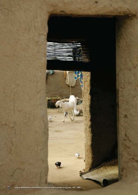
68<strong>Nature</strong>, distribution <strong>and</strong> evolution <strong>of</strong> poverty <strong>and</strong> <strong>in</strong>equality <strong>in</strong> Ug<strong>and</strong>a, 1992 - 2002
Appendix 1 | Expenditure-based small area estimationThe poverty mapp<strong>in</strong>g analysis undertaken was basedon a statistical technique, sometimes referred toas small area estimation. This approach comb<strong>in</strong>eshousehold welfare survey <strong>and</strong> census data (both collectedat approximately the same time) to estimate welfare orother <strong>in</strong>dicators for disaggregated geographic units such ascommunities. Researchers at the World Bank <strong>in</strong>itiated thisapproach <strong>in</strong> 1996 (Hentschel <strong>and</strong> Lanjouw, 1996) <strong>and</strong> the keymethodological paper is Elbers et al. (2003).The techniquescont<strong>in</strong>ue to be ref<strong>in</strong>ed with many collaborators <strong>and</strong> thereis now considerable reference material, most <strong>of</strong> which isavailable at www.worldbank.org. In this report, we give a brief<strong>and</strong> non--technical summary <strong>of</strong> the approach.The approach beg<strong>in</strong>s with the nationally representativehousehold welfare survey to acquire a reliable estimate <strong>of</strong>household expenditure (y). To calculate more specific povertymeasures l<strong>in</strong>ked to a poverty l<strong>in</strong>e, log-l<strong>in</strong>ear regressionsare estimated to model per capita expenditure us<strong>in</strong>g a set<strong>of</strong> explanatory variables (x) that are common to both thehousehold welfare survey <strong>and</strong> the census (e.g. householdsize, education, hous<strong>in</strong>g <strong>and</strong> <strong>in</strong>frastructure characteristics <strong>and</strong>demographic variables). These first-stage regression modelsare modelled at the lowest geographical level for which thehousehold welfare survey data is representative (Region),<strong>and</strong> a different first-stage model is estimated for each stratum(e.g. Region, urban <strong>and</strong> rural). Next, the estimated coefficientsfrom these regressions (<strong>in</strong>clud<strong>in</strong>g the estimated error termsassociated with those coefficients) are used to predict log percapita expenditure for every household <strong>in</strong> the census. Thesehousehold-unit data are then aggregated to small statisticalareas, such as sub-counties, to obta<strong>in</strong> robust estimates <strong>of</strong> thepercentage <strong>of</strong> households liv<strong>in</strong>g below the poverty l<strong>in</strong>e. Thesepoverty rates are used to produce a poverty map show<strong>in</strong>g thespatial distribution <strong>of</strong> poverty at the sub-county level, <strong>in</strong> thecase <strong>of</strong> Ug<strong>and</strong>a, which represents a significantly higher level<strong>of</strong> resolution than the region-level measures obta<strong>in</strong>able fromus<strong>in</strong>g the household welfare survey alone.In the first stage <strong>of</strong> the Ug<strong>and</strong>a analysis, variables with<strong>in</strong>the census <strong>and</strong> household survey were exam<strong>in</strong>ed <strong>in</strong> detail.The objective <strong>of</strong> this stage was to determ<strong>in</strong>e whether therewas a statistically similar distribution <strong>of</strong> the variables overhouseholds <strong>in</strong> the population census<strong>and</strong> <strong>in</strong> the household sample survey. Forexample, there are questions <strong>in</strong> both thepopulation census <strong>and</strong> <strong>in</strong> the householdsurvey about household size, level <strong>of</strong>education <strong>of</strong> the household head <strong>and</strong> type<strong>of</strong> hous<strong>in</strong>g. However, the exact questions<strong>and</strong> manner <strong>in</strong> which the answers arerecorded differ <strong>in</strong> some cases, e.g. theexact number <strong>of</strong> years <strong>of</strong> school<strong>in</strong>g for thehousehold head was asked <strong>and</strong> recorded<strong>in</strong> the survey, while whether they have aneducation at primary, secondary, or higherlevel is what was recorded <strong>in</strong> the census. Inmany cases, there were also discrepanciesbetween identically def<strong>in</strong>ed variables dueto regional variation <strong>in</strong> <strong>in</strong>terpretation,render<strong>in</strong>g certa<strong>in</strong> variables comparable <strong>in</strong>some regions <strong>and</strong> not <strong>in</strong> others.The next step was to <strong>in</strong>vestigate whetherthese common variables were statisticallysimilarly distributed over households <strong>in</strong>the population <strong>and</strong> those sampled by thesurvey. This assessment was based onthe follow<strong>in</strong>g statistics for each variableobta<strong>in</strong>ed from both the survey <strong>and</strong> thecensus for each stratum: (i) the mean, (ii)the st<strong>and</strong>ard error, (Hi) <strong>and</strong> the values forthe 1st, 5th, 10th, 25th, 50th, 75th, 90th, 95th<strong>and</strong> 99th percentiles. First, the census meanfor a particular variable was tested to seeif it lay with<strong>in</strong> the 95% confidence <strong>in</strong>tervalaround the household survey mean for thesame variable. Second, for dummy variables,means were checked to ensure they werenot smaller than 3 percent <strong>and</strong> not largerthan 97%, so that the variables constructedconta<strong>in</strong> some variation across households.The results <strong>of</strong> the comparison <strong>of</strong> variablemeans for the census <strong>and</strong> survey, by region<strong>and</strong> for urban <strong>and</strong> rural areas, are availablefrom the authors on request.<strong>Nature</strong>, distribution <strong>and</strong> evolution <strong>of</strong> poverty <strong>and</strong> <strong>in</strong>equality <strong>in</strong> Ug<strong>and</strong>a, 1992 - 2002 69