2000 - Draper Laboratory

More documents

Recommendations

Info

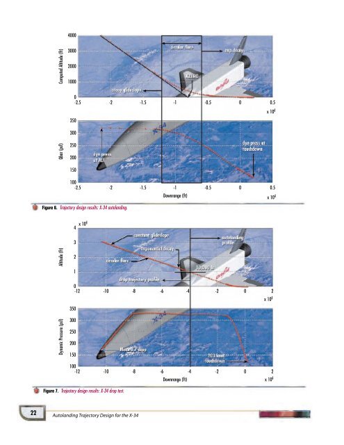
This method proved to be very robust. If the profile underconsideration is not within the physical envelope of the vehicle,then no solution will be found for Eqs. (26) and (27). In thiscase, the search for an acceptable angle of attack exceeds thelimits of the aerodynamic tables.This method of finding the control for a desired profile can beextended to include a higher-fidelity gravity field and higherordereffects due to a spinning, oblate earth. A thrust profilecould also be included, but the additional degree of freedomand additional constraints may alter the manner in which theequations are solved.TWO-POINT BOUNDARY VALUE PROBLEM FOR XZEROWe return to the problem of finding the intercept value of thesteep glideslope, XZERO, so that the terminal constraint ondynamic pressure is satisfied. To solve this two-point boundaryvalue problem, we employ a shooting technique. [5] Foreach estimate of XZERO, a trajectory is propagated by the procedureoutlined in the preceding section. This simulationyields the dynamic pressure and control history along the candidatealtitude profile specified by XZERO. The value of XZE-RO is changed via a secant root finding method in order tosatisfy the constraint on the touchdown dynamic pressure.Varying XZERO essentially determines downtrack distanceflown during autolanding. Decreasing XZERO decreases thelength of the autolanding trajectory as shown in Figure 5. Thisresults in a shorter time of flight so that less energy is dissipatedand the vehicle lands with a higher dynamic pressure.Figure 5.RESULTSEffect of changing XZERO.To demonstrate the trajectory design algorithms, the DRM5mission of the X-34 is used. This mission reaches a maximumspeed of Mach 2.7 before beginning the unpowered descentguidance. At the autolanding interface of 10,000 ft, the vehiclewill nominally have a dynamic pressure of 330 psf.The required touchdown dynamic pressure is 123 psf (whichequates to a ground speed of 203 kn). Using ALIP to solve thetwo-point boundary value problem for this condition yieldsan XZERO of 7865 ft. The final trajectory design and thedynamic pressure are shown in Figure 6. The upper part of thetrajectory has been omitted to show more detail during theflare segments. Notice that the dynamic pressure stays fairlyconstant during the steep glideslope due to the use of theequilibrium solution. The dynamic pressure decays during thecircular and exponential flares to reach the desired value.Obtaining this solution requires 12 s on a 300-MHz Pentium ina nonoptimized MATLAB environment. For a poor initial guessof XZERO, the results may take two or three times longer.High-fidelity X-34 simulation software was used to validatethe solution and assess the performance. The 6-degree-offreedommodel includes a spinning, oblate earth, sensor models,actuator models, and actual X-34 guidance, navigation,and control flight software. The altitude and dynamic pressurehistories are indistinguishable from the plots in Figure 6.EXTENDING THE METHOD BEYOND AUTOLANDINGThe success of the algorithms in designing trajectories motivatedan investigation as to the applicability of the techniquesto higher altitudes. The flight phase prior to autolanding iscalled Terminal Area Energy Management (TAEM), whichbegins at about Mach 3.5 and ends at ALI (10,000 ft) for the X-34. To extend the design approach into TAEM, the pattern ofthe autolanding flight segments (steep glideslope, circularflare, exponential flare, shallow glideslope) was repeated priorto the autolanding interface. Note that the shallow glideslopeof this series of geometric segments coincides with and isequal to the steep glideslope of the autolanding flight phases.This approach is demonstrated in Figure 7 for an unpowereddrop test of the X-34. In one of the early designs for DRM4, thevehicle is dropped from an L-1011 at Mach 0.7 and an altitudeof 35,000 ft. A new set of flight segments has been computedfor the trajectory above ALI. This required the solution of twoseparate two-point boundary value problems – one for thedrop (above ALI) and one for autolanding. The terminal constrainton the dynamic pressure for the upper segment wassimply the initial value for the autolanding trajectory (seeFigure 7). In theory, this approach of designing a trajectorywith the geometric segments as building blocks can continuewell into TAEM.CONCLUSIONSThe method employed by ALIP for constructing a trajectory ofwell-defined geometric segments holds great promise forrapid trajectory design of an onboard reference for the flightguidance system. The trajectory design algorithms are automatedand converge on a solution very quickly. Using theAutolanding Trajectory Design for the X-34 21
4000Computed Altitude (ft)3000<strong>2000</strong>10000-2.5 -2 -1.5 -1 -0.5 0 0.5x 10 4350300Qbar (psf)250200150100-2.5 -2 -1.5 -1 -0.5 0 0.5•Downrange (ft) x 10 4Figure 6. Trajectory design results: X-34 autolanding.4x 10 43Altitude (ft)210-12 -10 -8 -6 -4 -2 0 2x 10 4350Dynamic Pressure (psf)300250200150100-12 -10 -8 -6 -4 -2 0 2•Downrange (ft) x 10 4Figure 7. Trajectory design results: X-34 drop test.-22 Autolanding Trajectory Design for the X-34- --- -
Page 6 and 7: V 0 e jωt L R R R TL: (Z 0 ,β,I)C
Page 9 and 10: Figure 16 shows a fabricated "race-
Page 11 and 12: ACKNOWLEDGMENTS LEDGMENTSThe author
Page 13 and 14: aanan MillerRaanan Miller is a Seni
Page 15 and 16: The motivation for developing ALIP
Page 17 and 18: (4)where the state variables v and
Page 19: q’ = f 1 (q, α, h) (26)q = f 2 (
Page 23 and 24: eg H. Bartonbiographies biographies
Page 25 and 26: ActuatorsSensorsIntelligent Sensors
Page 27 and 28: Table 2. Potential sensors requirin
Page 29 and 30: Table 4. Comparison of single-chann
Page 31 and 32: Using many small I/O networks will
Page 33 and 34: Network Control ComputersTriple Twi
Page 35 and 36: Kaplesh KumarAnthony PetrovichTommy
Page 37 and 38: DESIGN CONSIDERATIONSThe overall go
Page 39 and 40: BIAS DRIFT STABILITYAn important re
Page 41 and 42: Hz291206002912050029120400291203002
Page 43 and 44: In order to show bias repeatability
Page 45 and 46: nthony PetrovichAnthony Petrovich i
Page 47 and 48: Ramses M. AgustinRami S. MangoubiRo
Page 49 and 50: v k is the sensor noise. In our cas
Page 51 and 52: The preceding performance criterion
Page 53 and 54: JET THRUST ESTIMATIONWe will first
Page 55 and 56: 1st measurement (nominal)0.010.0050
Page 57 and 58: 45004000350030002500Thrust (lb)2000
Page 59 and 60: amses AgustinbiographiesRamses Agus
Page 61 and 62: Jamie M. AndersonPeter A. Kerrebroc
Page 63 and 64: Figure 1. The Draper Laboratory VCU
Page 65 and 66: were adjusted to give good tracking
Page 67 and 68: 80604020Heading (deg)0-20-40-60-800
Page 69 and 70: Marc S. WeinbergII:"'JI.m-4..... 7.
Page 71 and 72:
where z i is measured from the arbi
Page 73 and 74:
L = beam lengthC = capacitance of e
Page 75 and 76:
3.02.52.0F/z ratio to linear1.51.00
Page 77 and 78:
The following pages contain the bib
Page 79 and 80:
errors. Numerical testing based on
Page 81 and 82:
of which are high performance and p
Page 83 and 84:
presented.The economic benefits of
Page 85 and 86:
over conventional analyzers. A plan
Page 87 and 88:
Smith, J.; Proulx, R.J.; Cefola, P.
Page 89 and 90:
using a dissolved wafer process wit
Page 91 and 92:
Donald E. GustafsonDavid J. LuciaAu
Page 93 and 94:
onald E. GustafsonbiographiesDonald
Page 95 and 96:
Greiff, Paul; Brezinski, PaulGetter
Page 97 and 98:
DOCTOR ROBERT D. MAURERDr. Maurer l
Page 99 and 100:
All Draper employees (excluding Off
Page 101:
Chauddhry, A.I.; Supervisors: Kang,
show all

2000 - Draper Laboratory

Create successful ePaper yourself

Delete template?

Save as template?