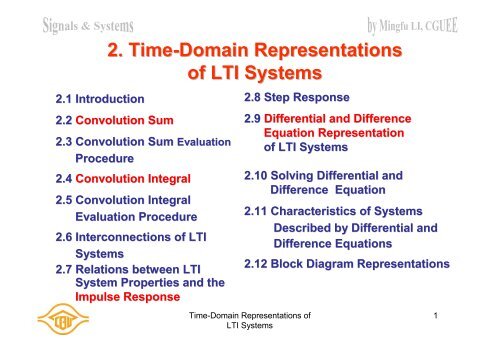
2. Time-Domain Representations of LTI Systems

2. Impulse Response of LTI System HOutput:Input x[n]LTI systemHyn H x n H x k n kk y n H x k n kk k 2.2 Convolution Sumy [ n] x[k]H{[n k]}Linearity(2.2)Output y[n]HomogeneityThe system output is a weighted sum of theresponse of the system to time-shifted impulses.For time-invariant system:H{ [n k]} h[ n k] (2.3)h[n] = H{[n]} impulseresponse of the LTI system Hk y [ n] x[k]h[n k](2.4)Convolution process:Fig. 2.2.Time-Domain Representations ofLTI Systems4

3. ConvolutionSum x n h n x k h n kk 2.2 Convolution Sumx[ 1][n 1]x[ 0] [n]x[ 1] n [ 1]x[ 2] n [ 2] kx [ n] x[k][n k]Time-Domain Representations ofLTI Systems5

2.3 Convolution Sum Evaluation ProcedureExample 2.2:Convolution Sum Evaluation by usingIntermediate Signaln3Consider a system with impulse response h n un 4Find the output of the system when the input is x [n] = u [n].Fig. 2.3 Fig. 2.3 depicts x[k] superimposed on the reflected and timeshiftedimpulse response h[nk].Find h[nk] :Time-Domain Representations ofLTI Systems9

2.3 Convolution Sum Evaluation Procedure1. When n < 0 :2. When n 0 :Time-Domain Representations ofLTI Systems10

2.3 Convolution Sum Evaluation ProcedureExample 2.3: Moving-Average System: Reflect-and-shiftConvolution Sum EvaluationThe output y[n] of the four-point moving-average system is related tothe input x[n] according to the formula31y n x n k4 k 0The impulse response h[n] of this system isobtained by letting x[n] = [n], which yields1h n u n u n4 4Fig. 2.4 (a).Determine the output of the system when theinput is the rectangular pulse defined as 10x n u n u nFig. 2.4 (b).Time-Domain Representations ofLTI Systems11

2.3 Convolution Sum Evaluation Procedure1. Refer to Fig. 2.4. Five intervals !2. 1’st interval : w n [k] = 01’st interval: n < 02’nd interval: 0 ≤n ≤33’rd interval: 3 < n ≤94th interval: 9 < n ≤125th interval: n > 12Time-Domain Representations ofLTI Systems12

2.3 Convolution Sum Evaluation Procedure3. 2’nd interval: 0 ≤n ≤34. 3’rd interval: 3 < n ≤95. 4th interval: 9 < n ≤12Time-Domain Representations ofLTI Systems13

2.3 Convolution Sum Evaluation Procedure6. 5th interval: n > 12Time-Domain Representations ofLTI Systems14

2. Impulse response of LTI system H :Output:2.4 Convolution Integral1. Weighted Superposition of Time-Shifted Functions x ( t) x()(t ) d y t H x t H x t d Input x(t)Time-Domain Representations ofLTI Systems LTI systemH3. h(t) = H{(t)} impulse response of the LTI system HIf the system is also time invariant, thenH{ (t )} h( t )(2.11)(2.10)y ( t) x()H{(t )} d y ( t) x()h(t ) d(2.12)4. Convolution integral:The shifting property of the impulse !(2.10)Fig. 2.9. x t h t x h t dLinearity propertyOutput y(t)A time-shifted impulse generates atime-shifted impulse response output24

2.5 Convolution Integral Evaluation Procedure1. Convolution Integral : y ( t)x( t)h( t) x()h(t ) d(2.13) h( )x(t ) dh(t)x( t)Commutative Law2. Convolution Evaluation Procedure :1) Graph both x() and h() .2) Reflect h() about = 0 to obtain h() and then shift h() by tunit to obtain h(t ) .3) Multiply x() and h(t ) .4) Increase the shift t (i.e., move h(t ) toward the right) until themathematical form for x()h(t ) changes.5) Discuss the values of t to obtain y(t) .Time-Domain Representations ofLTI Systems25

2.5 Convolution Integral Evaluation ProcedureExample 2.6: Reflect-and-shift Convolution EvaluationGiven x t u t 1 ut3 h t u t u t2Evaluate the convolution integral y(t) = x(t) h(t).1. Graph of x() and h(t ) :Fig. 2.11 (a).and as depicted in Fig. 2-10210,2. y( t)x( t)h( t) x ( )h(t ) dx()11 3h( t )1Time-Domain Representations ofLTI Systemst 2t 2 t t 2 t t t 226

2.5 Convolution Integral Evaluation Procedurey t0, t 1t 1, 1 t 35 t, 3 t 50, t 5Time-Domain Representations ofLTI Systems27

1. Parallel Connection of LTI Systems(2) Output :2.6 Interconnection of LTI Systems(1) Two LTI systems : Fig. 2.18(a).y( t) y ( t) y ( t)1 2x ( t) h ( t) x ( t) h ( t)1 2y( t) x( ) h ( t ) d x( ) h ( t )d1 21 2y( t) x( ) h ( t ) h ( t ) d x( ) h( t ) d x( t) h ( t)(3) Distributive property :x1 212( t)h( t)x( t)h( t)x( t){h ( t)h ( t)}(2.15)x1 212[ n]h[ n]x[ n]h[ n]x[ n]{h [ n]h [ n]}(2.16)Time-Domain Representations ofLTI Systemswhere h(t) = h 1 (t) + h 2 (t)Fig. 2.18(b)34

2.6 Interconnection of LTI Systems2. Cascade Connection of LTI Systems(1) Two LTI systems : Fig. 2.19(a).(2) The output is expressed in terms of z(t) as( t)z( t)h( t)(2.17)y2y(t) Substituting Eq. (2.19) for z(t) into Eq. (2.18) givesy( t) x( v) h ( v) h ( t ) dvd z()h2 ( t )1 2Define h(t) = h 1 (t) h 2 (t), thenh( t v ) h ( ) h ( t v ) d1 2d(2.18)(2.19)Fig. 2.19(b).Since z(t) is the output of the first system, so it can be expressed asx( )h 1()x()h1( dz ( ))y ( t))Change of variable= x() h1()h2( t dd y( t)x()h(t ) dx( t)h( t)(2.21)(2.20)Time-Domain Representations ofLTI Systems35

2.6 Interconnection of LTI Systems(3) Associative property :{ x(t)h1(t)}h2(t)x( t){h1( t)h2(t)}{2x[n]h1[n]}h2[n]x[ n]{h1[n]h[ n]}(4) Commutative property:Write h(t) = h 1 (t) h 2 (t) as the integralh( t) h ( ) h ( t ) d1 2 h( t)h1 ( t ) h2( )dh2(t)h1(t)Time-Domain Representations ofLTI SystemsChange of variable= t Fig. 2.19(c).Interchanging the order of the LTI systems in the cascade withoutaffecting the result:x( t) h ( t) h ( t) x ( t) h ( t) h ( t) , 1 2 2 1Commutative property forcontinuous-time case :h t)h( t)h( t)h( )1( 2 2 1t(2.24)(2.22)(2.25)(2.23)Commutative property fordiscrete-time case :h n]h[ n]h[ n]h[ ]1[ 2 2 1n(2.26)36

Example 2.11: Equivalent System to Four Interconnected SystemsConsider the interconnection of four LTI systems, as depicted in Fig.2.20. The impulse responses of the systems areh [ n]u[ n],1 2h [ n ] u [ n 2] u [ n ], h [ n][ n 2],[ ] n[ ].3 and h4 n u nFind the impulse response h[n] of the overall system.2.6 Interconnection of LTI Systems1. Parallel combination of h 1 [n] andh 2 [n] : h 12 [n] = h 1 [n] + h 2 [n]Fig. 2.21 (a).Time-Domain Representations ofLTI Systems37

2.6 Interconnection of LTI Systems2. h 12 [n] is in series with h 3 [n] : h 123 [n] = h 12 [n] h 3 [n]h 123 [n] = (h 1 [n] + h 2 [n]) h 3 [n]Fig. 2.21 (b).3. h 123 [n] is in parallel with h 4 [n] : h[n] = h 123 [n] h 4 [n]h[ n] ( h [ n] h [ n]) h [ n] h [ n],Fig. 2.21 (c).1 2 3 4Thus, substitute the specified forms of h 1 [n] and h 2 [n] to obtainh [ ] [ ] [ 2] [ ]12n u n u n u nu [ n 2]Convolving h 12 [n] with h 3 [n] givesh [ n] u [ n 2] [ n 2]123u [ n][ ] 1 nh n u [ n ].Time-Domain Representations ofLTI Systems38

2.6 Interconnection of LTI SystemsTable 2.1:summarizes the interconnection properties presented inthis section.Time-Domain Representations ofLTI Systems(2.27)39

2.7 Relations Between LTISystem Properties and the Impulse Response1. Memoryless LTI Systems(1) The output of a discrete-time LTI system :y[ n] h [ n] x [ n] h[ k] x[ n k]ky[n] h[ 2]x[n 2]h[ 1]x[n 1]h[0] x[n]h[1] x[n 1]h[2] x[n 2] (2) To be memoryless, y[n] must depend only on x[n] andtherefore cannot depend on x[nk] for k 0.A discrete-time LTI system is memoryless if and only ifh[ k] c [ k]Continuous-time system :(1) Output:y( t) h( ) x( t ) d,c is an arbitrary constant(2) A continuous-time LTI system ismemoryless if and only ifh( ) c ( )(2.27)c is an arbitrary constantTime-Domain Representations ofLTI Systems40

2.7 Relations Between LTISystem Properties and the Impulse Response2. Causal LTI SystemsThe output of a causal LTI system depends only on past or presentvalues of the input.Discrete-time system :1. Convolution sum : y[ n] h [ 2] x[ n 2] h [ 1] x[ n 1] h [0] x[ n]2. For a discrete-time causal LTIsystem,h[ k] 0 for k 0Continuous-time system:1. Convolution integral:y( t) h( ) x( t ) d.h [1] x[ n 1] h [2] x[ n 2] .2. For a continuous-time causal LTI system,h( ) 0 for 0Time-Domain Representations ofLTI Systems3. Convolution sum in new form:y[ n] h[ k] x[ n k].k 03. Convolution integral innew form:y( t) h( ) x( t ) d.041

2.7 Relations Between LTISystem Properties and the Impulse Response3. Stable LTI SystemsA system is BIBO stable if the output is guaranteed to be bounded forevery bounded input.Discrete-time case : Input x[ n] Mx Output : y[ n] My(1) The magnitude of output :y[ n] h[ n] x [ n] h[ k] x[ n k] y[ n] h[ k] x[ n k]k y[ n] h[ k] x[ n k] ab a bk (2) Assume that the input is bounded, i.e.,x[ n] Mx x[ n k ] Mxand it follows that xk y [ n]Mh[k](2.28)k a b a bHence, the output is bounded,or y[n] ≤for all n, providedthat the impulse response ofthe system is absolutelysummable.Time-Domain Representations ofLTI Systems42

2.7 Relations Between LTISystem Properties and the Impulse Response(3) Condition for impulse response of a stable discrete-time LTI system :k h[ k] .Continuous-time case :Condition for impulse response of a stable continuous-time LTIsystem : h( ) d.0Example 2.12: Properties of the First-Order Recursive SystemThe first-order system is described by the difference equationy[ n] y[ n 1] x [ n]and has the impulse responsenh[ n] u[ n]Is this system causal, memoryless, and BIBO stable?Time-Domain Representations ofLTI Systems43

2.7 Relations Between LTISystem Properties and the Impulse Response1. The system is causal, since h[n] = 0 for n < 0.2. The system is not memoryless, since h[n] 0 for n > 0.3. Stability : Checking whether the impulse response is absolutely summable?kkh[ k] if and only if < 1k k 0 k 0◆ Special case : A system can be unstable even though the impulseresponse has a finite value.1. Ideal integrator :2. Ideal accumulator : ty ( t)x()d(2.29)Input : x() = (), then theoutput is y(t) = h(t) = u(t).h(t) is not absolutely integrableIdeal integrator is not stable!nk y[ n] x[ k]Impulse response : h[n] = u[n]h[n] is not absolutely summableIdeal accumulator is not stable!Time-Domain Representations ofLTI Systems44

2.7 Relations Between LTISystem Properties and the Impulse Response4. Invertible Systems and DeconvolutionA system is invertible if the input to the system can be recovered fromthe output except for a constant scale factor.(1) h(t) = impulse response of LTI system, Fig. 2.24.(2) h inv (t) = impulse response of LTI inverse system(3) The process of recovering x(t) from h(t) x(t) is termeddeconvolution.(4) An inverse system performs deconvolution.x t h t h t x tin( ) ( ( ) v ( )) ( ).invh( t) h ( t) ( t)(2.30)inv(5) Discrete-time case: h[ n]h[ n] [ n](2.31)Continuous-timecaseTime-Domain Representations ofLTI Systems45

2.7 Relations Between LTISystem Properties and the Impulse Response★ Table 2.2 summarizes the relation between LTI system propertiesand impulse response characteristics.Time-Domain Representations ofLTI Systems48

2.8 Step Response1. The step response is defined as the output dueto a unit step input signal.2. Discrete-time LTI system:Let h[n] = impulse response and s[n] = step response.s[ n] h [ n]* u[ n] h[ k] u[ n k].k 3. Since u[nk] = 0 for k > n and u[nk] = 1for k ≤n, we havens[ n] h[ k].k The step response is the running sum of the impulseresponse.Time-Domain Representations ofLTI Systems49

2.8 Step Response◆ Continuous-time LTI system :s ( t)h( t)u( t) h()u(t ) dh()d(2.34)The step response s(t) is the running integral of the impulseresponse h(t).◆ Express the impulse response in terms of the stepresponse ash[ n] s [ n] s [ n 1] and h( t) s( t)dtExample 2.14: RC Circuit: Step ResponseThe impulse response of the RC circuit depicted in Fig. 2.12 ist1 RCh( t) e u( t)RCFind the step response of the circuit.tdTime-Domain Representations ofLTI Systems50

1. Step response:t 1 RCs( t) e u( ) d.RC2.8 Step ResponseFig. 2.25Time-Domain Representations ofLTI Systems51

2.9 Differential and DifferenceEquation Representations of LTI Systems1. Linear constant-coefficient differential equation :Nk 0akddtThe order of the differential or difference equation is (N, M),representing the number of energy storage devices in the system.Ex. RLC circuit depicted in Fig. 2.26.1. Input = voltage source x(t),output = loop current2. KVL Eq. :kky(t)Mk 0bkddtkkx(t)(2.35)d 1 tRy t L y t y d x tdt C Input = x(t), output = y(t)2. Linear constant-coefficient difference equation :Nk 0aky[n k] Mk 0bkx[n k](2.36)Input = x[n], output = y[n]Often, N M, and theorder is describedusing only N.Time-Domain Representations ofLTI Systems52

2.9 Differential and DifferenceEquation Representations of LTI Systems1 d2d dC dt2dt dt y t R y t L y t x tN = 2Ex. Accelerator modeled in Section 1.10 :22 d dny t y t y t x t2Q dt dtn where y(t) = the position of the proof mass, x(t) = externalacceleration.Time-Domain Representations ofLTI SystemsN = 2Ex. Second-order difference equation :1y[n]y[ n 1] y[n 2]x[ n]2x[n 1]4(2.37) N = 2Difference equations are easily rearranged to obtain recursiveformulas for computing the current output of the system from theinput signal and the past outputs.53

2.9 Differential and DifferenceEquation Representations of LTI SystemsEx. Eq. (2.36) can be rewritten asMN1 1y n b x n k a y n k ak0 k0 a0k 1kEx. Consider computing y[n] for n 0 from x[n] for thesecond-order difference equation (2.37).1. Eq. (2.37) can be rewritten as1y[ n]x[ n]2x[n 1]y[ n 1] y[n 2]42. Computing y[n] for n 0:1y[ 0] x[0] 2x[1]y[ 1] y[2]4(2.39)1y[1] x[1] 2x[0]y[0] y[1]4 (2.40)(2.38)Time-Domain Representations ofLTI Systems1y x x y y4 2 2 2 1 1 01y x x y y4 3 3 2 2 2 154

2.9 Differential and DifferenceEquation Representations of LTI Systems◆ Initial conditions : y[1] and y[2].◆ The initial conditions for Nth-order difference equation are the Nvalues , 1 ,..., 1 ,y N y N y◆ The initial conditions for Nth-order differential equation are the Nvalues2 N 1d d dy t y t y t y t , , ..., t0 , 2 N 1dt t0 dt t0 dtt0Time-Domain Representations ofLTI Systems55

2.9 Differential and DifferenceEquation Representations of LTI SystemsExample 2.15: Recursive Evaluation of a Difference EquationFind the first two output values y[0] and y[1] for the system describedby Eq. (2.38), assuming that the input is x[n] = (1/2) n u[n] and the initialconditions are y[1] = 1 and y[2] = 2.1. Substitute the appropriate values into Eq. (2.39) to obtain2. Substitute for y[0] in Eq. (2.40) to findTime-Domain Representations ofLTI Systems56

2.10 SolvingDifferential and Difference EquationsComplete solution: y = y (h) + y (p) ,1. The Homogeneous SolutionContinuous-time case:1. Homogeneous differential equation :2. Homogeneous solution :y( h)( t)Ni0c eir ti(2.41)k3. Characteristic eq. : a kr 0(2.42)k 0Discrete-time case:1. Homogeneous differential equation :2. Homogeneous solution :y( h)NNTime-Domain Representations ofLTI Systemsy (h) = homogeneous solution,y (p) = particular solutionNNk 0k 0kdaky tkdtk ha y n k h00Coefficients c i isdetermined by I.C.nN[ n]ciri(2.43) 3. Characteristic eq. : ka kr 0(2.44)i1Nk 062

If a root r j is repeated p timesin characteristic eqs., thecorresponding solutions arer t r t p1r tContinuous-time case : e , te , ..., t eExample 2.17: RC Circuit: Homogeneous Solutionj j jDiscrete-time case: r , nr , ..., n rn n p1nj j jThe RC circuit depicted in Fig. 2.30 is described by the differentialequationdy t RC y t x tdtDetermine the homogeneous solution of this equation.2.10 SolvingDifferential and Difference Equations1. Homogeneous Eq. :2. Homo. Sol. :3. Characteristic eq. :4. Homogeneous solution:Time-Domain Representations ofLTI Systems63

Example 2.18: First-Order Recursive System: Homogeneous SolutionFind the homogeneous solution for the first-order recursive systemdescribed by the difference equation y n y n 1 x n2.10 SolvingDifferential and Difference Equations1. Homogeneous Eq. :2. Homo. Sol. :3. Characteristic eq. :4. Homogeneous solution :Time-Domain Representations ofLTI Systems64

2.10 SolvingDifferential and Difference Equations2. The Particular SolutionA particular solution is usually obtained by assuming an output ofthe same general form as the input. Table 2.3Time-Domain Representations ofLTI Systems65

Example 2.19: First-Order Recursive System (Continued):Particular SolutionFind a particular solution for the first-order recursive system describedy n y n 1x nby the difference equation if the input is x[n] = (1/2) n .2.10 SolvingDifferential and Difference Equations1. Particular solution form :2. Substituting y (p) [n] and x[n] into the given difference Eq. :c p( 12)13. Particular solution :(2.45)Both sides of above eq. aremultiplied by (1/2) nTime-Domain Representations ofLTI Systems66

2.10 SolvingDifferential and Difference EquationsExample 2.20: RC Circuit (continued): Particular SolutionConsider the RC circuit of Example 2.17 and depicted in Fig. 2.30. Finda particular solution for this system with an input x(t) = cos( 0 t).1. Differential equation :2. Particular solution form :3. Substituting y (p) (t) and x(t) = cos( 0 t) into the given differential Eq. :c cos( t ) c sin( t ) RC c sin( t) RC c cos( t) cos( t)1 2 0 1 0 0 2 0 04. Coefficients c 1 and c 2 :5. Particular solution :Time-Domain Representations ofLTI Systems67

2.10 SolvingDifferential and Difference Equations3. The Complete SolutionComplete solution: y = y (h) + y (p)y (h) = homogeneous solution, y (p) = particular solutionThe procedure for finding complete solution of differential ordifference equations is summarized as follows :Procedure 2.3: Solving a Differential or Difference equation1. Find the form of the homogeneous solution y (h) from the roots ofthe characteristic equation.2. Find a particular solution y (p) by assuming that it is of the sameform as the input, yet is independent of all terms in thehomogeneous solution.3. Determine the coefficients in the homogeneous solution so thatthe complete solution y = y (h) + y (p) satisfies the initial conditions.★ Note that the initial translation is needed in some cases.Time-Domain Representations ofLTI Systems68

2.10 SolvingDifferential and Difference EquationsExample 2.21: First-Order Recursive System : Complete SolutionFind the complete solution for the first-order recursive systemdescribed by the difference equation 1y[ n] y[n 1]x[ n](2.46)4if the input is x[n] = (1/2) n u[n] and the initial condition is y[1] = 8.1. Homogeneous sol. : 2. Particular solution :3. Complete solution : (2.47)4. Coefficient c 1 determined by I.C. :I.C. : y 0 x 0 1 4 y 1We substitute y[0] = 3into Eq. (2.47), yielding5. Final solution :for n 0Time-Domain Representations ofLTI Systems69

2.10 SolvingDifferential and Difference EquationsExample 2.22: RC Circuit (continued): Complete ResponseFind the complete response of the RC circuit depicted in Fig. 2.30 toan input x(t) = cos(t)u(t) V, assuming normalized values R = 1 and C = 1 F and assuming that the initial voltage across thecapacitor is y(0 ) = 2 V.1. Homogeneous sol. :2. Particular solution: p 1RCy t cos2 t sin2 t V1 RC 1 RC 3. Complete solution : 0= 1R = 1 , C = 1 F4. Coefficient c 1 determined by I.C. : y(0 ) = y(0+ )0 1 1 12 ce cos0 sin 0 c c = 3/22 2 2Time-Domain Representations ofLTI Systems5. Final solution:70

2.11 Characteristics of Systems Describedby Differential and Difference EquationsComplete solution: y = y (n) + y (f)y (n) = natural response, y (f) = forced response1. The Natural Response (Zero(Input)Example 2.24: RC Circuit (continued): Natural ResponseThe system In Example 2.17 is described by the differential equationdy t RC y t x tdtFind the natural response of the this system, assuming thaty(0) = 2 V, R = 1 and C = 1 F. 1. Homogeneous sol. :2. I.C.: y(0) = 2 V3. Natural Response :Time-Domain Representations ofLTI Systems71

2.11 Characteristics of Systems Describedby Differential and Difference EquationsExample 2.25: First-Order Recursive System : Natural ResponseThe system in Example 2.21 is described by the difference equation1y n yn 1xn and the initial condition is y[1] = 8.4Find the natural response of this system.1. Homogeneous sol. :2. I.C.: y[1] = 83. Natural Response :Time-Domain Representations ofLTI Systems72

2.11 Characteristics of Systems Describedby Differential and Difference Equations2. The Forced Response (only valid for t 0 or n 0)The forced response is the system output due to the input signalassuming zero initial conditions.The at-rest conditions for a discrete-time system, y[N] = 0, …,y[1] = 0, must be translated forward to times n = 0, 1, …, N1before solving for the undetermined coefficients, such as whenone is determining the complete solution.Example 2.26: First-Order Recursive System : Forced ResponseThe system in Example 2.21 is described by the difference equation1y n yn 1xn4Find the forced response of this system if the input isx[n] = (1/2) n u[n].Time-Domain Representations ofLTI Systems73

2.11 Characteristics of Systems Describedby Differential and Difference Equations1. Complete solution :2. I.C.: Translate the at-rest condition y[1] to time n = 03. Finding c 1 :4. Forced response:Time-Domain Representations ofLTI Systems74

2.11 Characteristics of Systems Describedby Differential and Difference EquationsExample 2.27: RC Circuit (continued): Forced ResponseThe system In Example 2.17 is described by the differential equationdy t RC y t x tdtFind the forced response of the this system, assuming that x(t) =cos(t)u(t) V, R = 1 and C = 1 F.t1 11. Complete solution : y t ce cost sintV2 22. I.C. : y(0 ) = y(0 + ) = 0 c = 1/23. Forced response:From Example 2.22Time-Domain Representations ofLTI Systems75

2.11 Characteristics of Systems Describedby Differential and Difference Equations3. The Impulse ResponseRelation between step response and impulse response1. Continuous-time case : 2. Discrete-time case :dh n s [ n] s [ n 1]h( t) s( t)dt4. Linearity and Time InvarianceForced response LinearityInputx 1x 2x 1 + x 2Forcedresponsey 1(f)y 2(f)y 1(f)+ y 2(f)Initial Cond.I 1I 2I 1 + I 2Time-Domain Representations ofLTI SystemsNatural response LinearityNaturalresponsey 1(n)y 2(n)y 1(n)+ y 2(n)The complete response of an LTI system is not time invariant.Response due to initial condition will not shift with a time shiftof the input.76

2.11 Characteristics of Systems Describedby Differential and Difference Equations5. Roots of the Characteristic EquationRoots of characteristic equationForced response, natural response, stability, and response time.★ BIBO Stable:n1. Discrete-time case : r boundedr 1, for alliiii2. Continuous-time case : er t boundede r i0 ri1and e r i0 The system is said to be on the verge of instability.Time-Domain Representations ofLTI Systems77

End of Chapter 2Time-Domain Representations ofLTI Systems83