DIFFERENTIAL GEOMETRY: A First Course in Curves and Surfaces

DIFFERENTIALGEOMETRY:A First Course inCurves and SurfacesPreliminary VersionSummer, 2006Theodore ShifrinUniversity of GeorgiaDedicated to the memory of Shiing-Shen Chern,my adviser and friendc○2006 Theodore ShifrinNo portion of this work may be reproduced in any form without writtenpermission of the author.

§1. Examples, Arclength Parametrization 3(e) Now consider the twisted cubic in R 3 , illustrated in Figure 1.3, given byα(t) =(t, t 2 ,t 3 ), t ∈ R.Its projections in the xy-, xz-, and yz-coordinate planes are, respectively, y = x 2 , z = x 3 ,and z 2 = y 3 (the cuspidal cubic).(f) Our next example is a classic called the cycloid: Itisthe trajectory of a dot on a rollingwheel (circle). Consider the illustration in Figure 1.4. Assuming the wheel rolls withoutOPtaFigure 1.4slipping, the distance it travels along the ground is equal to the length of the circular arcsubtended by the angle through which it has turned. That is, if the radius of the circle is aand it has turned through angle t, then the point of contact with the x-axis, Q, isat unitsto the right. The vector from the origin to the point P can be expressed as the sum of thePOQCPaCt a cos ta sin tFigure 1.5three vectors −→ OQ, −→ QC, and −→ CP (see Figure 1.5):−→OP = −→ OQ + −→ QC + −→ CPand hence the function=(at, 0)+(0,a)+(−a sin t, −a cos t),α(t) =(at − a sin t, a − a cos t) =a(t − sin t, 1 − cos t),t ∈ Rgives a parametrization of the cycloid.(g) A (circular) helix is the screw-like path of a bug as it walks uphill on a right circular cylinderat a constant slope or pitch. If the cylinder has radius a and the slope is b/a, wecan imaginedrawing a line of that slope on a piece of paper 2πa units long, and then rolling the paperup into a cylinder. The line gives one revolution of the helix, as we can see in Figure 1.6. Ifwe take the axis of the cylinder to be vertical, the projection of the helix in the horizontalplane is a circle of radius a, and so we obtain the parametrization α(t) =(a cos t, a sin t, bt).

4 Chapter 1. Curves2πb2πaFigure 1.6Brief review of hyperbolic trigonometric functions. Just as the circle x 2 + y 2 = 1 isparametrized by (cos θ, sin θ), the portion of the hyperbola x 2 − y 2 =1lying to the right ofthe y-axis, as shown in Figure 1.7, is parametrized by (cosh t, sinh t), wherecosh t = et + e −tand sinh t = et − e −t.22By analogy with circular trigonometry, we set tanh t = sinh t1and secht =cosh t cosh t . The(cosh t, sinh t)Figure 1.7following formulas are easy to check:cosh 2 t − sinh 2 t =1, tanh 2 t + sech 2 t =1sinh ′ (t) =cosh t, cosh ′ (t) =sinh t, tanh ′ (t) =sech 2 t, sech ′ (t) =− tanh t secht.

§1. Examples, Arclength Parametrization 5(h) When a uniform and flexible chain hangs from two pegs, its weight is uniformly distributedalong its length. The shape it takes is called a catenary. 1 As we ask the reader to check inExercise 9, the catenary is the graph of f(x) =C cosh(x/C), for any constant C>0. ThisFigure 1.8curve will appear numerous times in this course.Example 2. One of the more interesting curves that arises “in nature” is the tractrix. 2 Thetraditional story is this: A dog is at the end of a 1-unit leash and buries a bone at (0, 1) as hisowner begins to walk down the x-axis, starting at the origin. The dog tries to get back to the bone,so he always pulls the leash taut as he is dragged along the tractrix by his owner. His pulling theleash taut means that the leash will be tangent to the curve. When the master is at (t, 0), let the(0,1)▽(x,y)tθFigure 1.9dog’s position be (x(t),y(t)), and let the leash make angle θ(t) with the positive x-axis. Then wehave x(t) =t + cos θ(t), y(t) =sin θ(t), sotan θ(t) = dydx = y′ (t)x ′ (t) = cos θ(t)θ′ (t)1 − sin θ(t)θ ′ (t) .Therefore, θ ′ (t) =sin θ(t). Separating variables and integrating, we have ∫ dθ/ sin θ = ∫ dt, andso t = − ln(csc θ + cot θ) +c for some constant c. Since θ = π/2 when t =0,wesee that c =0.Now, since csc θ + cot θ = 1+cos θ 2 cos 2 (θ/2)== cot(θ/2), we can rewrite this assin θ 2 sin(θ/2) cos(θ/2)t =lntan(θ/2). Thus, we can parametrize the tractrix byα(θ) = ( cos θ +lntan(θ/2), sin θ ) ,π/2 ≤ θ

6 Chapter 1. CurvesAlternatively, since tan(θ/2) = e t ,wehavesin θ =2sin(θ/2) cos(θ/2) =2et1+e 2t = 2e t = secht+ e−t cos θ = cos 2 (θ/2) − sin 2 (θ/2) = 1 − e2t1+e 2t = e−t − e te t = − tanh t,+ e−t and so we can parametrize the tractrix instead byβ(t) = ( t − tanh t, secht), t ≥ 0. ▽The fundamental concept underlying the geometry of curves is the arclength of a parametrizedcurve.Definition. If α: [a, b] → R 3 is a parametrized curve, then for any a ≤ t ≤ b, wedefine itsarclength from a to t to be s(t) =∫ ta‖α ′ (u)‖du.arclength of its trajectory—is the integral of its speed.That is, the distance a particle travels—theAn alternative approach is to start with the followingDefinition. Let α: [a, b] → R 3 be a (continuous) parametrized curve. Given a partition P ={a = t 0

§1. Examples, Arclength Parametrization 7Now, using this definition, we can prove that the distance a particle travels is the integral ofits speed. We will need to use the result of Exercise A.2.4.Proposition 1.1. Let α: [a, b] → R 3 be a piecewise-C 1 parametrized curve. Thenlength(α) =∫ ba‖α ′ (t)‖dt.Proof. Forany partition P of [a, b], we havek∑k∑∫ til(α, P) = ‖α(t i ) − α(t i−1 )‖ =α ′ (t)dt∥ t i−1∥ ≤so length(α) ≤i=1∫ bai=1k∑i=1‖α ′ (t)‖dt. The same holds on any interval.∫ tit i−1‖α ′ (t)‖dt =∫ ba‖α ′ (t)‖dt,Now, for a ≤ t ≤ b, define s(t) tobethe arclength of the curve α on the interval [a, t]. Thenfor h>0wehave‖α(t + h) − α(t)‖h≤s(t + h) − s(t)h≤ 1 h∫ t+ht‖α ′ (u)‖du,since s(t + h) − s(t) isthe arclength of the curve α on the interval [t, t + h]. (See Exercise 8 for thefirst inequality.) NowTherefore, by the squeeze principle,‖α(t + h) − α(t)‖lim= ‖α ′ 1(t)‖ = limh→0 + hh→0 + hs(t + h) − s(t)lim= ‖α ′ (t)‖.h→0 + h∫ t+ht‖α ′ (u)‖du.A similar argument works for h

8 Chapter 1. CurvesAn important observation from a theoretical standpoint is that any regular parametrized curvecan be reparametrized by arclength. For if α is regular, the arclength function s(t) =∫ ta‖α ′ (u)‖duis an increasing function (since s ′ (t) =‖α ′ (t)‖ > 0 for all t), and therefore has an inverse functiont = t(s). Then we can consider the parametrizationNote that the chain rule tells us thatβ(s) =α(t(s)).β ′ (s) =α ′ (t(s))t ′ (s) =α ′ (t(s))/s ′ (t(s)) = α ′ (t(s))/‖α ′ (t(s))‖is everywhere a unit vector; in other words, β moves with speed 1.EXERCISES 1.1*1. Parametrize the unit circle (less the point (−1, 0)) by the length t indicated in Figure 1.11.(x,y)(−1,0)tFigure 1.11♯ 2.Consider the helix α(t) =(a cos t, a sin t, bt). Calculate α ′ (t), ‖α ′ (t)‖, and reparametrize α byarclength.3. Let α(t) = ( √3 1cos t + √ 1 12sin t, √3 1cos t, √3 cos t − √ 12sin t ) .reparametrize α by arclength.Calculate α ′ (t), ‖α ′ (t)‖, and*4. Parametrize the graph y = f(x), a ≤ x ≤ b, and show that its arclength is given by thetraditional formula∫ b √length = 1+ ( f ′ (x) ) 2 dx.a5. a. Show that the arclength of the catenary α(t) =(t, cosh t) for 0 ≤ t ≤ b is sinh b.b. Reparametrize the catenary by arclength. (Hint: Find the inverse of sinh by using thequadratic formula.)*6. Consider the curve α(t) =(e t ,e −t , √ 2t). Calculate α ′ (t), ‖α ′ (t)‖, and reparametrize α byarclength, starting at t =0.

§1. Examples, Arclength Parametrization 97. Find the arclength of the tractrix, given in Example 2, starting at (0, 1) and proceeding to anarbitrary point.♯ 8.Let P, Q ∈ R 3 and let α: [a, b] → R 3 be any parametrized curve with α(a) =P , α(b) =Q.Let v = Q − P . Prove that length(α) ≥‖v‖, sothat the line segment from P to Q gives theshortest possible path. (Hint: Consider∫ baα ′ (t) · vdt and use the Cauchy-Schwarz inequalityu · v ≤‖u‖‖v‖. Ofcourse, with the alternative definition on p. 6, it’s even easier.)9. Consider a uniform cable with density δ hanging in equilibrium. As shown in Figure 1.12, thetension forces T(x +∆x), −T(x), and the weight of the piece of cable lying over [x, x +∆x]all balance. If the bottom of the cable is at x =0,T 0 is the magnitude of the tension there,T(x+∆x)θ +∆θ−T(x)θ −gδ∆sxx+∆xFigure 1.12and the cable is the graph y = f(x), show that f ′′ (x) = gδ √1+fT ′ (x) 2 . (Remember that0tan θ = f ′ (x).) Letting ∫ C = T 0 /gδ, show that f(x) =C cosh(x/C) +c for some constant c.du(Hint: To integrate √ , make the substitution u = sinh v.)1+u 210. As shown in Figure 1.13, Freddy Flintstone wishes to drive his car with square wheels along astrange road. How should you design the road so that his ride is perfectly smooth, i.e., so thatthe center of his wheel travels in a horizontal line? (Hints: Start with a square with verticesOCQPFigure 1.13at (±1, ±1), with center C at the origin. If α(s) =(x(s),y(s)) is an arclength parametrization

10 Chapter 1. Curvesof the road, starting at (0, −1), consider the vector −→ OC = −→ OP + −→ PQ+ −→ QC, where P = α(s) isthe point of contact and Q is the midpoint of the edge of the square. Use −→ QP = sα ′ (s) and thefact that −→ QC is a unit vector orthogonal to −→ QP . Express the fact that C moves horizontallyto show that s = − y′ (s)x ′ ;you will need to differentiate unexpectedly. Now use the result of(s)Exercise 4 to find y = f(x). Also see the hint for Exercise 9.)⎧⎨( )t, t sin(π/t) , t ≠011. Show that the curve α(t) =has infinite length on [0, 1]. (Hint: Considerl(α, P) with P = {0, 1/N, 2/(2N − 1), 1/(N − 1),...,1/2, 2/3,⎩(0, 0), t =01}.)12. Prove that no four distinct points on the twisted cubic (see Example 1(e)) lie on a plane.13. (a special case of a recent American Mathematical Monthly problem) Suppose α: [a, b] → R 2is a smooth parametrized plane curve (perhaps not arclength-parametrized). Prove that if thechord length ‖α(s) − α(t)‖ depends only on |s − t|, then α must be a (subset of) a line or acircle. (How many derivatives of α do you need to use?)2. Local Theory: Frenet FrameWhat distinguishes a circle or a helix from a line is their curvature, i.e., the tendency of thecurve to change direction. We shall now see that we can associate to each smooth (C 3 ) arclengthparametrizedcurve α a natural “moving frame” (an orthonormal basis for R 3 chosen at each pointon the curve, adapted to the geometry of the curve as much as possible).We begin with a fact from vector calculus which will appear throughout this course.Lemma 2.1. Suppose f, g :(a, b) → R 3 are differentiable and satisfy f(t) · g(t) =const for allt. Then f ′ (t) · g(t) =−f(t) · g ′ (t). Inparticular,‖f(t)‖ = const if and only if f(t) · f ′ (t) =0 for all t.Proof. Since a function is constant on an interval if and only if its derivative is everywherezero, we deduce from the product rule,(f · g) ′ (t) =f ′ (t) · g(t)+f(t) · g ′ (t),that if f · g is constant, then f · g ′ = −f ′ · g. Inparticular, ‖f‖ is constant if and only if ‖f‖ 2 = f · fis constant, and this occurs if and only if f · f ′ =0. □Remark. This result is intuitively clear. If a particle moves on a sphere centered at the origin,then its velocity vector must be orthogonal to its position vector; any component in the directionof the position vector would move the particle off the sphere. Similarly, suppose f and g haveconstant length and a constant angle between them. Then in order to maintain the constant angle,as f turns towards g, wesee that g must turn away from f at the same rate.Using Lemma 2.1 repeatedly, we now construct the Frenet frame of suitable regular curves. Weassume throughout that the curve α is parametrized by arclength. Then, for starters, α ′ (s) isthe

§2. Local Theory: Frenet Frame 11unit tangent vector to the curve, which we denote by T(s). Since T has constant length, T ′ (s) will beorthogonal to T(s). Assuming T ′ (s) ≠ 0, define the principal normal vector N(s) =T ′ (s)/‖T ′ (s)‖and the curvature κ(s) =‖T ′ (s)‖. Sofar, we haveT ′ (s) =κ(s)N(s).If κ(s) =0,the principal normal vector is not defined. Assuming κ ≠0,wecontinue. Define thebinormal vector B(s) =T(s) × N(s). Then {T(s), N(s), B(s)} form a right-handed orthonormalbasis for R 3 .Now, N ′ (s) must be a linear combination of T(s), N(s), and B(s). But we know from Lemma2.1 that N ′ (s) · N(s) = 0 and N ′ (s) · T(s) = −T ′ (s) · N(s) = −κ(s). We define the torsionτ(s) =N ′ (s) · B(s). This gives usN ′ (s) =−κ(s)T(s)+τ(s)B(s).Finally, B ′ (s) must be a linear combination of T(s), N(s), and B(s). Lemma 2.1 tells us thatB ′ (s) · B(s) =0,B ′ (s) · T(s) =−T ′ (s) · B(s) =0,and B ′ (s) · N(s) =−N ′ (s) · B(s) =−τ(s). Thus,In summary, we have:B ′ (s) =−τ(s)N(s).Frenet formulasT ′ (s) =N ′ (s) =−κ(s)T(s)B ′ (s) =κ(s)N(s)+ τ(s)B(s)−τ(s)N(s)The skew-symmetry of these equations is made clearest when we state the Frenet formulas inmatrix form: ⎡ ⎤ ⎡⎤ ⎡⎤| | | | | | 0 −κ(s) 0⎢ ⎣ T ′ (s) N ′ (s) B ′ ⎥ ⎢⎥ ⎢⎥(s) ⎦ = ⎣ T(s) N(s) B(s) ⎦ ⎣ κ(s) 0 −τ(s) ⎦ .| | | | | | 0 τ(s) 0Indeed, note that the coefficient matrix appearing on the right is skew-symmetric. This is the casewhenever we differentiate an orthogonal matrix depending on a parameter (s in this case). (SeeExercise A.1.4.)Note that, by definition, the curvature, κ, isalways nonnegative; the torsion, τ, however, has asign, as we shall now see.Example 1. Consider the helix, given by its arclength parametrization (see Exercise 1.1.2)α(s) = ( a cos(s/c),asin(s/c), bs/c ) , where c = √ a 2 + b 2 . Then we haveT(s) = 1 ( )−a sin(s/c),acos(s/c),bcT ′ (s) = 1 ( ) a ( )−a cos(s/c), −a sin(s/c), 0 = − cos(s/c), − sin(s/c), 0c 2 }{{} c 2.} {{ }κN

12 Chapter 1. CurvesSummarizing,κ(s) = a c 2 =Now we deal with B and the torsion:aa 2 + b 2 and N(s) = ( − cos(s/c), − sin(s/c), 0 ) .B(s) =T(s) × N(s) = 1 c(b sin(s/c), −b cos(s/c),a)B ′ (s) = 1 c 2 (b cos(s/c),bsin(s/c), 0)= −bc 2 N(s),so we infer that τ(s) = bc 2 = ba 2 + b 2 .Note that both the curvature and the torsion are constants. The torsion is positive when thehelix is “right-handed” (b >0) and negative when the helix is “left-handed” (b

§2. Local Theory: Frenet Frame 13Using the more casual—but convenient—Leibniz notation for derivatives,dTdt = dTdTdsdT= υκN or κN =ds dt ds = dt= 1 ds υExample 2. Let’s calculate the curvature of the tractrix (see Example 2 in Section 1). Usingthe first parametrization, we have α ′ (θ) =(− sin θ + csc θ, cos θ), and sodtdTdt .υ(θ) =‖α ′ (θ)‖ = √ (− sin θ + csc θ) 2 + cos 2 θ = √ csc 2 θ − 1=− cot θ.(Note the negative sign because π 2≤ θ0 and (sin θ, − cos θ) isaunit vector we conclude thatκ(θ) =− tan θ and N(θ) =(sin θ, − cos θ).Later on we will see an interesting geometric consequence of the equality of the curvature and the(absolute value of) the slope. ▽Example 3. Let’s calculate the “Frenet apparatus” for the parametrized curveα(t) =(3t − t 3 , 3t 2 , 3t + t 3 ).We begin by calculating α ′ and determining the unit tangent vector T and speed υ:Nowα ′ (t) =3(1 − t 2 , 2t, 1+t 2 ),υ(t) =‖α ′ (t)‖ =3 √ (1 − t 2 ) 2 +(2t) 2 +(1+t 2 ) 2 =3 √ 2(1 + t 2 ) 2 =3 √ 2(1 + t 2 )T(t) = √ 1 12 1+t 2 (1 − t2 , 2t, 1+t 2 )= √ 1 ( )1 − t22 1+t 2 , 2t1+t 2 , 1 .κN = dT dTds = dtdsdtso= 1 dTυ(t) dt(1 −4t√2 (1 + t 2 ) 2 , 2(1 − )t2 )(1 + t 2 ) 2 , 01=3 √ 2(1 + t 2 )1=3 √ 1 2√ ·2(1 + t 2 ) 2 1+t 2} {{ }κ(−2t1+t 2 , 1 − )t21+t 2 , 0 .} {{ }NHere we have factored out the length of the derivative vector and left ourselves with a unit vectorin its direction, which must be the principal normal N; the magnitude that is left must be theand

14 Chapter 1. Curvescurvature κ. Insummary, so far we haveκ(t) =13(1 + t 2 ) 2 and N(t) =(−2t1+t 2 , 1 − )t21+t 2 , 0 .Next we find the binormal B by calculating the cross productB(t) =T(t) × N(t) = √ 1 (− 1 − t22 1+t 2 , − 2t )1+t 2 , 1 .And now, at long last, we calculate the torsion by differentiating B:so τ(t) =κ(t) =−τN = dB dBds = dtds13(1 + t 2 ) 2 . ▽dt= 1 dBυ(t) dt()1 4t√2 (1 + t 2 ) 2 , 2(t2 − 1)(1 + t 2 ) 2 , 01=3 √ 2(1 + t 2 )(1= −3(1 + t 2 )} {{ 2 −2t1+t}2 , 1 − )t21+t 2 , 0 ,} {{ }τNNow we see that curvature enters naturally when we compute the acceleration of a movingparticle. Differentiating the formula (∗) onp.12, we obtainα ′′ (t) =υ ′ (t)T(s(t)) + υ(t)T ′ (s(t))s ′ (t)= υ ′ (t)T(s(t)) + υ(t) 2( κ(s(t))N(s(t)) ) .Suppressing the variables for a moment, we can rewrite this equation as(∗∗)α ′′ = υ ′ T + κυ 2 N.The tangential component of acceleration is the derivative of speed; the normal component (the“centripetal acceleration” in the case of circular motion) is the product of the curvature of the pathand the square of the speed. Thus, from the physics of the motion we can recover the curvature ofthe path:Proposition 2.2. Forany regular parametrized curve α, wehave κ = ‖α′ × α ′′ ‖‖α ′ ‖ 3 .Proof. Since α ′ × α ′′ =(υT) × (υ ′ T + κυ 2 N)=κυ 3 T × N and κυ 3 > 0, we obtain κυ 3 =‖α ′ × α ′′ ‖, and so κ = ‖α ′ × α ′′ ‖/υ 3 ,asdesired. □We next proceed to study various theoretical consequences of the Frenet formulas.Proposition 2.3. A space curve is a line if and only if its curvature is everywhere 0.Proof. The general line is given by α(s) =sv + c for some unit vector v and constant vectorc. Then α ′ (s) =T(s) =v is constant, so κ =0. Conversely, if κ =0,then T(s) =T 0 is a constant∫ svector, and, integrating, we obtain α(s) = T(u)du = sT 0 + c for some constant vector c. This0is, once again, the parametric equation of a line. □

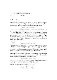
§2. Local Theory: Frenet Frame 15Example 4. Suppose all the tangent lines of a space curve pass through a fixed point. Whatcan we say about the curve? Without loss of generality, we take the fixed point to be the originand the curve to be arclength-parametrized by α. Then for every s we have α(s) =λ(s)T(s) forsome scalar function λ. Differentiating, we haveT(s) =α ′ (s) =λ ′ (s)T(s)+λ(s)T ′ (s) =λ ′ (s)T(s)+λ(s)κ(s)N(s).Then (λ ′ (s) − 1)T(s) +λ(s)κ(s)N(s) =0, so, since T(s) and N(s) are linearly independent, weinfer that λ(s) =s + c for some constant c and κ(s) =0. Therefore, the curve must be a linethrough the fixed point. ▽Somewhat more challenging is the followingProposition 2.4. A space curve is planar if and only if its torsion is everywhere 0. The onlyplanar curves with nonzero constant curvature are (portions of) circles.Proof. If a curve lies in a plane P, then T(s) and N(s) span the plane P 0 parallel to Pand passing through the origin. Therefore, B = T × N is a constant vector (the normal toP 0 ), and so B ′ = −τN = 0, from which we conclude that τ =0. Conversely, if τ =0,thebinormal vector B is a constant vector B 0 .Now, consider the function f(s) =α(s) · B 0 ;wehavef ′ (s) =α ′ (s) · B 0 = T(s) · B(s) =0,and so f(s) =c for some constant c. This means that α liesin the plane x · B 0 = c.We leave it to the reader to check in Exercise 2a. that a circle of radius a has constant curvature1/a. (This can also be deduced as a special case of the calculation in Example 1.) Now suppose aplanar curve α has constant curvature κ 0 . Consider the auxiliary function β(s) =α(s)+ 1 N(s).κ 0Then we have β ′ (s) =α ′ (s) + 1 (−κ 0 (s)T(s)) = T(s) − T(s) =0. Therefore β is a constantκ 0function, say β(s) =P for all s. Now we claim that α is a (subset of a) circle centered at P , for‖α(s) − P ‖ = ‖α(s) − β(s)‖ =1/κ 0 . □We have already seen that a circular helix has constant curvature and torsion. We leave itto the reader to check in Exercise 10 that these are the only curves with constant curvature andtorsion. Somewhat more interesting are the curves for which τ/κ is a constant.A generalized helix is a space curve with κ ≠0all of whose tangent vectors make a constantangle with a fixed direction. As shown in Figure 2.2, this curve lies on a generalized cylinder,formed by taking the union of the lines (rulings) in that fixed direction through each point of thecurve. We can now characterize generalized helices by the followingProposition 2.5. A curve is a generalized helix if and only if τ/κ is constant.Proof. Suppose α is an arclength-parametrized generalized helix. Then there is a (constant)unit vector A with the property that T · A = cos θ for some constant θ. Differentiating, we obtainκN · A =0,whence N · A =0. Differentiating yet again, we have(†)(−κT + τB) · A =0.Now, note that A lies in the plane spanned by T and B, and thus B · A = ± sin θ. Thus, we inferfrom equation (†) that τ/κ = ± cot θ, which is indeed constant.

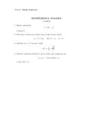
16 Chapter 1. CurvesFigure 2.2Conversely, if τ/κ is constant, set τ/κ = cot θ for some angle θ ∈ (0,π). Set A(s) =cos θT(s)+sin θB(s). Then A ′ (s) =(κ cos θ − τ sin θ)N(s) =0, soA(s) isaconstant unit vector A, andT(s) · A = cos θ is constant, as desired. □Example 5. In Example 3 we saw a curve α with κ = τ, sofrom the proof of Proposition 2.5 wesee that the curve should make a constant angle θ = π/4 with the vector A = 1 √2(T+B) =(0, 0, 1)(as should have been obvious from the formula for T alone). We verify this in Figure 2.3 by drawingα along with the vertical cylinder built on the projection of α onto the xy-plane. ▽Figure 2.3

§2. Local Theory: Frenet Frame 17The Frenet formulas actually characterize the local picture of a space curve.Proposition 2.6 (Local canonical form). Let α beasmooth (C 3 or better) arclength-parametrizedcurve. If α(0) = 0, then for s near 0, wehave() ( )α(s) = s − κ2 0κ06 s3 + ... T(0) +2 s2 + κ′ (0κ0 τ)06 s3 + ... N(0) +6 s3 + ... B(0).(Here κ 0 , τ 0 , and κ ′ 0 denote, respectively, the values of κ, τ, and κ′ at 0, and lims→0.../s 3 =0.)Proof. Using Taylor’s Theorem, we writeα(s) =α(0) + sα ′ (0) + 1 2 s2 α ′′ (0) + 1 6 s3 α ′′′ (0) + ...,where lims→0.../s 3 =0. Now,α(0) = 0, α ′ (0) = T(0), and α ′′ (0) = T ′ (0) = κ 0 N(0). Differentiatingagain, we have α ′′′ (0) = (κN) ′ (0) = κ ′ 0 N(0) + κ 0(−κ 0 T(0) + τ 0 B(0)). Substituting, we obtainas required.α(s) =sT(0) + 1 2 s2 κ 0 N(0) + 1 ( 6 s3 −κ 2 0T(0) + κ ′ 0N(0) + κ 0 τ 0 B(0) ) + ...() ( )= s − κ2 0κ06 s3 + ... T(0) +2 s2 + κ′ (0κ0 τ)06 s3 + ... N(0) +6 s3 + ... B(0),□We now introduce three fundamental planes at P = α(0):(i) the osculating plane, spanned by T(0) and N(0),(ii) the rectifying plane, spanned by T(0) and B(0), and(iii) the normal plane, spanned by N(0) and B(0).We see that, locally, the projections of α into these respective planes look like(i) (u, (κ 0 /2)u 2 + ...)(ii) (u, (κ 0 τ 0 /6)u 3 + ...), and(iii) (u 2 ,( √2τ03 √ κ 0)u 3 + ...),where limu→0.../u 3 =0.Thus, the projections of α into these planes look locally as shown in Figure2.4. The osculating (“kissing”) plane is the plane that comes closest to containing α near P (seeNBBTTNosculating plane rectifying plane normal planeFigure 2.4

18 Chapter 1. Curvesalso Exercise 23); the rectifying (“straightening”) plane is the one that comes closest to flatteningthe curve near P ; the normal plane is normal (perpendicular) to the curve at P . (Cf. Figure 1.3.)EXERCISES 1.21. Compute the curvature of the following arclength-parametrized curves:a. α(s) = ( √2 1 1cos s, √2 cos s, sin s )b. α(s) = (√ 1+s 2 , ln(s + √ 1+s 2 ) )*c. α(s) = ( 13 (1 + s)3/2 , 1 3 (1 − s)3/2 1, √2 s ) , s ∈ (−1, 1)2. Calculate the unit tangent vector, principal normal, and curvature of the following curves:a. a circle of radius a: α(t) =(a cos t, a sin t)b. α(t) =(t, cosh t)c. α(t) =(cos 3 t, sin 3 t), t ∈ (0,π/2)3. Calculate the Frenet apparatus (T, κ, N, B, and τ) ofthe following curves:*a. α(s) = ( 13 (1 + s)3/2 , 1 3 (1 − s)3/2 1, √2 s ) , s ∈ (−1, 1)b. α(t) = ( 12 et (sin t + cos t), 1 2 et (sin t − cos t),e t)*c. α(t) = (√ 1+t 2 ,t,ln(t + √ 1+t 2 ) )d. α(t) =(e t cos t, e t sin t, e t )e. α(t) =(cosh t, sinh t, t)♯ 4. Prove that the curvature of the plane curve y = f(x) isgiven by κ =♯ *5.|f ′′ |(1 + f ′2 ) 3/2 .Use Proposition 2.2 and the second parametrization of the tractrix given in Example 2 ofSection 1 to recompute the curvature.*6. By differentiating the equation B = T × N, derive the equation B ′ = −τN.♯ 7. Suppose α is an arclength-parametrized space curve with the property that ‖α(s)‖ ≤‖α(s 0 )‖ =R for all s sufficiently close to s 0 . Prove that κ(s 0 ) ≥ 1/R. (Hint: Consider the functionf(s) =‖α(s)‖ 2 . What do you know about f ′′ (s 0 )?)8. Let α be a regular (arclength-parametrized) curve with nonzero curvature. The normal line toα at α(s) isthe line through α(s) with direction vector N(s). Suppose all the normal lines toα pass through a fixed point. What can you say about the curve?9. a. Prove that if all the normal planes of a curve pass through a particular point, then thecurve lies on a sphere. (Hint: Apply Lemma 2.1.)*b. Prove that if all the osculating planes of a curve pass through a particular point, then thecurve is planar.10. Prove that if κ = κ 0 and τ = τ 0 are nonzero constants, then the curve is a (right) circular helix.(Hint: The only solutions of the differential equation y ′′ +k 2 y =0are y = c 1 cos(kt)+c 2 sin(kt).)

§2. Local Theory: Frenet Frame 19Remark. It is an amusing exercise to give a and b (in our formula for the circular helix)in terms of κ 0 and τ 0 .*11. Proceed as in the derivation of Proposition 2.2 to show thatτ = α′ · (α ′′ × α ′′′ )‖α ′ × α ′′ ‖ 2 .12. Let α be a C 4 arclength-parametrized curve with κ ≠0. Prove that α is a generalized helix ifand only if α ′′ · (α ′′′ × α (iv) )=0. (Here α (iv) denotes the fourth derivative of α.)13. Suppose κτ ≠0atP .Ofall the planes containing the tangent line to α at P , show that α lieslocally on both sides only of the osculating plane.14. Let α be a regular curve with κ ≠0atP . Prove that the planar curve obtained by projectingα into its osculating plane at P has the same curvature at P as α.15. A closed, planar curve C is said to have constant breadth µ if the distance between paralleltangent lines to C is always µ. (No, C needn’t be a circle. See Figure 2.5.) Assume for therest of this problem that the curve is C 2 and κ ≠0.(the Wankel engine design)Figure 2.5a. Let’s call two points with parallel tangent lines opposite. Prove that if C has constantbreadth µ, then the chord joining opposite points is normal to the curve at both points.(Hint: If β(s) isopposite α(s), then β(s) =α(s)+λ(s)T(s)+µN(s). First explain whythe coefficient of N is µ; then show that λ = 0.)b. Prove that the sum of the reciprocals of the curvature at opposite points is equal to µ.(Warning: If α is arclength-parametrized, β is quite unlikely to be.)16. Let α and β be two regular curves defined on [a, b]. We say β is an involute of α if, for eacht ∈ [a, b],(i) β(t) lies on the tangent line to α at α(t), and(ii) the tangent vectors to α and β at α(t) and β(t), respectively, are perpendicular.Reciprocally, we also refer to α as an evolute of β.a. Suppose α is arclength-parametrized. Show that β is an involute of α if and only ifβ(s) =α(s)+(c − s)T(s) for some constant c (here T(s) =α ′ (s)). We will normally refer

20 Chapter 1. Curvesto the curve β obtained with c =0asthe involute of α. Ifyou were to wrap a stringaround the curve α, starting at s =0,the involute is the path the end of the string followsas you unwrap it, always pulling the string taut, as illustrated in the case of a circle inFigure 2.6.PθFigure 2.6b. Show that the involute of a helix is a plane curve.c. Show that the involute of a catenary is a tractrix. (Hint: You do not need an arclengthparametrization!)d. If α is an arclength-parametrized plane curve, prove that the curve β given byβ(s) =α(s)+ 1κ(s) N(s)is the unique evolute of α lying in the plane of α. Prove, moreover, that this curve isregular if κ ′ ≠0. (Hint: Go back to the original definition.)17. Find the involute of the cycloid α(t) =(t + sin t, 1 − cos t), t ∈ [−π, π], using t =0asyourstarting point. Give a geometric description of your answer.18. Let α be a curve parametrized by arclength with κ, τ ≠0.a. Suppose α lies on the surface of a sphere centered at the origin (i.e., ‖α(s)‖ = const forall s). Prove that(⋆)( ( )τ 1 1 ′ ) ′κ + =0.τ κ(Hint: Write α = λT + µN + νB for some functions λ, µ, and ν, differentiate, and use thefact that {T, N, B} is a basis for R 3 .)b. Prove the converse: If α satisfies the differential equation (⋆), then α lies on the surfaceof some sphere. (Hint: Using the values of λ, µ, and ν you obtained in part a, show thatα − (λT + µN + νB) isaconstant vector, the candidate for the center of the sphere.)19. Two distinct parametrized curves α and β are called Bertrand mates if for each t, the normalline to α at α(t) equals the normal line to β at β(t). An example is pictured in Figure 2.7.Suppose α and β are Bertrand mates.

§2. Local Theory: Frenet Frame 21Figure 2.7a. If α is arclength-parametrized, show that β(s) =α(s)+r(s)N(s) and r(s) =const. Thus,corresponding points of α and β are a constant distance apart.b. Show that, moreover, the angle between the tangent vectors to α and β at correspondingpoints is constant. (Hint: If T α and T β are the unit tangent vectors to α and βrespectively, consider T α · T β .)c. Suppose α is arclength-parametrized and κτ ≠0. Show that α has a Bertrand mate β ifand only if there are constants r and c so that rκ + cτ =1.d. Given α, prove that if there is more than one curve β so that α and β are Bertrand mates,then there are infinitely many such curves β and this occurs if and only if α is a circularhelix.20. (See Exercise 19.) Suppose α and β are Bertrand mates. Prove that the torsion of α and thetorsion of β at corresponding points have constant product.21. Suppose Y is a C 2 vector function on [a, b] with ‖Y‖ =1and Y, Y ′ , and Y ′′ everywhere linearly∫ t (independent. For any nonzero constant c, define α(t) =c Y(u)×Y ′ (u) ) du, t ∈ [a, b]. Provethat the curve α has constant torsion 1/c. (Hint: Show that B = ±Y.)22. a. Let α be an arclength-parametrized plane curve. We create a “parallel” curve β by takingβ = α + εN (for a fixed small positive value of ε). Explain the terminology and expressthe curvature of β in terms of ε and the curvature of α.b. Now let α be an arclength-parametrized space curve. Show that we can obtain a “parallel”curve β by taking β = α + ε ( (cos θ)N + (sin θ)B ) for an appropriate function θ. Howmany such parallel curves are there?c. Sketch such a parallel curve for a circular helix α.23. Suppose α is an arclength-parametrized curve, P = α(0), and κ(0) ≠0. Use Proposition 2.6to establish the following:*a. Let Q = α(s) and R = α(t). Show that the plane spanned by P , Q, and R approachesthe osculating plane of α at P as s, t → 0.b. The osculating circle at P is the limiting position of the circle passing through P , Q, andR as s, t → 0. Prove that the osculating circle has center Z = P + ( 1/κ(0) ) N(0) andradius 1/κ(0).c. The osculating sphere at P is the limiting position of the sphere through P and threeneighboring points on the curve, as the latter points tend to P independently. Prove thata

22 Chapter 1. Curvesthe osculating sphere has center Z = P + ( 1/κ(0) ) N(0)+ ( 1/τ(0)(1/κ) ′ (0) ) B(0) and radius√(1/κ(0)) 2 +(1/τ(0)(1/κ) ′ (0)) 2 .d. How is the result of part c related to Exercise 18?24. a. Suppose β is a plane curve and C s is the circle centered at β(s) with radius r(s). Assumingβ and r are differentiable functions, show that the circle C s is contained inside the circleC t whenever t>sif and only if ‖β ′ (s)‖ ≤r ′ (s) for all s.b. Let α be arclength-parametrized plane curve and suppose κ is a decreasing function. Provethat the osculating circle at α(s) lies inside the osculating circle at α(t) whenever t>s.(See Exercise 23 for the definition of the osculating circle.)25. Suppose the front wheel of a bicycle follows the arclength-parametrized plane curve α. Determinethe path β of the rear wheel, 1 unit away, as shown in Figure 2.8. (Hint: If the frontFigure 2.8wheel is turned an angle θ from the axle of the bike, start by writing α − β in terms of θ, T,and N. Your goal should be a differential equation that θ must satisfy. Note that the path ofthe rear wheel will obviously depend on the initial condition θ(0). In all but the simplest ofcases, it may be impossible to solve the differential equation explicitly.)3. Some Global Results3.1. Space Curves. The fundamental notion in geometry (see Section 1 of the Appendix) isthat of congruence: When do two figures differ merely by a rigid motion? If the curve α ∗ is obtainedfrom the curve α by performing a rigid motion (composition of a translation and a rotation), thenthe Frenet frames at corresponding points differ by that same rigid motion, and the twisting of theframes (which is what gives curvature and torsion) should be the same. (Note that a reflection willnot affect the curvature, but will change the sign of the torsion.)Theorem 3.1 (Fundamental Theorem of Curve Theory). Two space curves C and C ∗ are congruent(i.e., differ by a rigid motion) if and only if the corresponding arclength parametrizationsα, α ∗ :[0,L] → R 3 have the property that κ(s) =κ ∗ (s) and τ(s) =τ ∗ (s) for all s ∈ [0,L].Proof. Suppose α ∗ =Ψ◦α for some rigid motion Ψ: R 3 → R 3 ,soΨ(x) =Ax + b for someb ∈ R 3 and some 3 × 3 orthogonal matrix A with det A > 0. Then α ∗ (s) = Aα(s) +b, so‖α ∗′ (s)‖ = ‖Aα ′ (s)‖ =1,since A is orthogonal. Therefore, α ∗ is likewise arclength-parametrized,

§3. Some Global Results 23and T ∗ (s) = AT(s). Differentiating again, κ ∗ (s)N ∗ (s) = κ(s)AN(s). Since A is orthogonal,‖AN(s)‖ is a unit vector, and so N ∗ (s) =AN(s) and κ ∗ (s) =κ(s). But then B ∗ (s) =T ∗ (s) ×N ∗ (s) = AT(s) × AN(s) = A(T(s) × N(s)) = AB(s), inasmuch as orthogonal matrices maporthonormal bases to orthonormal bases and det A>0 insures that orientation is preserved as well.Last, B ∗′ (s) =−τ ∗ (s)N ∗ (s) and B ∗′ (s) =AB ′ (s) =−τ(s)AN(s) =−τ(s)N ∗ (s), so τ ∗ (s) =τ(s),as required.Conversely, suppose κ = κ ∗ and τ = τ ∗ . Wenow define a rigid motion Ψ as follows. Letb = α ∗ (0) − α(0), and let A be the unique orthogonal matrix so that AT(0) = T ∗ (0), AN(0) =N ∗ (0), and AB(0) = B ∗ (0). A also has positive determinant, since both orthonormal bases areright-handed. Set ˜α =Ψ◦α. Wenow claim that α ∗ (s) = ˜α(s) for all s ∈ [0,L]. Note, by ourargument in the first part of the proof, that ˜κ = κ = κ ∗ and ˜τ = τ = τ ∗ . Considerf(s) = ˜T(s) · T ∗ (s)+Ñ(s) · N∗ (s)+ ˜B(s) · B ∗ (s).We now differentiate f, using the Frenet formulas.f ′ (s) = ( ˜T′ (s) · T ∗ (s)+ ˜T(s) · T ∗′ (s) ) + ( Ñ ′ (s) · N ∗ (s)+Ñ(s) · N∗′ (s) )+ ( ˜B′ (s) · B ∗ (s)+ ˜B(s) · B ∗′ (s) )= κ(s) ( Ñ(s) · T ∗ (s)+ ˜T(s) · N ∗ (s) ) − κ(s) ( ˜T(s) · N ∗ (s)+Ñ(s) · T∗ (s) )=0,+ τ(s) ( ˜B(s) · N ∗ (s)+Ñ(s) · B∗ (s) ) − τ(s) ( Ñ(s) · B ∗ (s)+ ˜B(s) · N ∗ (s) )since the first two terms cancel and the last two terms cancel. By construction, f(0) = 3, sof(s) =3forall s ∈ [0,L]. Since each of the individual dot products can be at most 1, the onlyway the sum can be 3 for all s is for each to be 1 for all s, and this in turn can happen onlywhen ˜T(s) =T ∗ (s), Ñ(s) =N ∗ (s), and ˜B(s) =B ∗ (s) for all s ∈ [0,L]. In particular, since˜α ′ (s) = ˜T(s) =T ∗ (s) =α ∗′ (s) and ˜α(0) = α ∗ (0), it follows that ˜α(s) =α ∗ (s) for all s ∈ [0,L], aswe wished to show. □Remark. The latter half of this proof can be replaced by asserting the uniqueness of solutionsof a system of differential equations, as we will see in a moment. Also see Exercise A.3.1 for amatrix-computational version of the proof we just did.Example 1. We now see that the only curves with constant κ and τ are circular helices.▽Perhaps more interesting is the existence question: Given continuous functions κ, τ :[0,L] → R(with κ everywhere positive), is there a space curve with those as its curvature and torsion? Theanswer is yes, and this is an immediate consequence of the fundamental existence theorem fordifferential equations, Theorem 3.1 of the Appendix. That is, we let⎡⎤⎡⎤| | |0 −κ(s) 0⎢F (s) = ⎣T(s) N(s) B(s)| | |⎥⎢⎦ and K(s) = ⎣κ(s) 0 −τ(s)0 τ(s) 0Then integrating the linear system of ordinary differential equations F ′ (s) =F (s)K(s), F (0) = F 0 ,gives us the Frenet frame everywhere along the curve, and we recover α by integrating T(s).⎥⎦ .

24 Chapter 1. CurvesWe turn now to the concept of total curvature of a closed space curve, which is the integral of itscurvature. That is, if α: [0,L] → R 3 is an arclength-parametrized curve with α(0) = α(L), its totalcurvature is∫ L0κ(s)ds. This quantity can be interpreted geometrically as follows: The Gauss mapof α is the map to the unit sphere, Σ, given by the unit tangent vector T: [0,L] → Σ; its image,Γ, is classically called the tangent indicatrix of α. Observe that—provided the Gauss map is one-TFigure 3.1to-one—the length of Γ is the total curvature of α, since length(Γ) =∫ L0‖T ′ (s)‖ds =∫ L0κ(s)ds.A preliminary question to ask is this: What curves Γ in the unit sphere can be the Gauss map ofsome closed space curve α? Since α(s) =α(0) +condition is that∫ L0∫ s0T(u)du, wesee that a necessary and sufficientT(s)ds = 0. (Note, however, that this depends on the arclength parametrizationof the original curve and is not a parametrization-independent condition on the image curveΓ ⊂ Σ.) We do, nevertheless, have the following geometric consequence of this condition. For any(unit) vector A, wehave0=A ·∫ L0T(s)ds =∫ L0(T(s) · A)ds,and so the average value of T · A must be 0. In particular, the tangent indicatrix must cross thegreat circle with normal vector A. That is, if the curve Γ is to be a tangent indicatrix, it must be“balanced” with respect to every direction A. Itisnatural to ask for the shortest curve(s) withthis property.If ξ ∈ Σ, let ξ ⊥ denote the (oriented) great circle with normal vector ξ.Proposition 3.2 (Crofton’s formula). Let Γ be apiecewise-C 1 curve on the sphere. Thenlength(Γ) = 1 ∫#(Γ ∩ ξ ⊥ )dξ4 Σ= π × (the average number of intersections of Γ with all great circles).(Here dξ represents the usual element of surface area on Σ.)Proof. We leave this to the reader in Exercise 11.□Remark. Although we don’t stop to justify it here, the set of ξ for which #(Γ ∩ ξ ⊥ )isinfiniteis a set of measure zero, and so the integral makes sense.

§3. Some Global Results 25Applying this to the case of the tangent indicatrix of a closed space curve, we deduce thefollowing classical result.Theorem 3.3 (Fenchel). The total curvature of any closed space curve is at least 2π, andequality holds if and only if the curve is a convex, planar curve.Proof. Let Γ be the tangent indicatrix of our space curve. ∫ For almost every ξ ∈ Σwehave#(Γ ∩ ξ ⊥ ) ≥ 2, and so it follows from Proposition 3.2 that κds = length(Γ) ≥ 1 (2)(4π) =2π.4Now, we claim that if Γ is a connected, closed curve in Σ of length ≤ 2π, then Γ lies in a closedhemisphere. It will follow, then, that if Γ is a tangent indicatrix of length 2π, itmust be a greatcircle. (For if Γ lies in the hemisphere A · x ≥ 0,∫ Lgreat circle A · x = 0.) It follows that the curve is planar.0T(s) · Ads =0forces T · A =0,soΓis thePNQΓ 1Γ 1Figure 3.2To prove the claim, we proceed as follows. Suppose length(Γ) ≤ 2π. Choose P and Q in Γso that the arcs Γ 1 = PQ ⌢and Γ 2 = QP ⌢have the same length. Choose N bisecting the shortergreat circle arc from P to Q, asshown in Figure 3.2. For convenience, we rotate the picture sothat N is the north pole of the sphere. Suppose now that the curve Γ 1 were to enter the southernhemisphere; let Γ 1 denote the reflection of Γ 1 across the north pole (following arcs of great circlethrough N). Now, Γ 1 ∪ Γ 1 is a closed curve containing a pair of antipodal points and therefore islonger than a great circle. (See Exercise 1.) Since Γ 1 ∪ Γ 1 has the same length as Γ, we see thatlength(Γ) > 2π, which is a contradiction. Therefore Γ indeed lies in the northern hemisphere. □We now sketch the proof of a result that has led to many interesting questions in higherdimensions. We say a simple closed space curve is knotted if we cannot fill it in with a disk.Theorem 3.4 (Fary-Milnor). If a simple closed space curve is knotted, then its total curvatureis at least 4π.Sketch of proof. Suppose the total curvature of C is less than 4π. Then the average number#(Γ∩ξ ⊥ ) < 4. Since this is generically an even number ≥ 2 (whenever the great circle isn’t tangentto Γ), there must be an open set of ξ’s for which we have #(Γ∩ξ ⊥ )=2. Choose one such, ξ 0 . Thismeans that the tangent vector to C is only perpendicular to ξ 0 twice, so the function f(x) =x · ξ 0has only two critical points. That is, the planes perpendicular to ξ 0 will (by Rolle’s Theorem)

26 Chapter 1. Curvesintersect C either in a line segment or in a single point (at the top and bottom); that is, by movingthese planes from the bottom of C to the top, we fill in a disk, so C is unknotted. □3.2. Plane Curves. We conclude this chapter with some results on plane curves. First, itmakes sense to consider curvature with a sign. Rather than proceeding as we did in Section 2,instead, given an arclength-parametrized curve α, define N(s) sothat {T(s), N(s)} is a righthandedbasis for R 2 (i.e., one turns counterclockwise from T(s) toN(s)), and then set T ′ (s) =κ(s)N(s), as before. So κ>0 when T is twisting counterclockwise and κ0}, U 2 = {(x, y) ∈ S 1 :x0}, and U 4 = {(x, y) ∈ S 1 : y

§3. Some Global Results 27Define θ(0) so that T(0) = ( cos θ(0), sin θ(0) ) . Let S = {s ∈ [0,L]:θ is defined and C 1 on[0,s]}, and let s 0 = sup S. Suppose first that s 0 0sothat0T(s) ∈ U i for all s with |s − s 0 |

28 Chapter 1. Curvesh(s,t)α(t)α(s)α(0)T(0)Figure 3.4Recall that one of the ways of characterizing a convex function f : R → R is that its graph lieon one side of each of its tangent lines. So we make the followingDefinition. The regular closed plane curve α is convex if it lies on one side of its tangent lineat each point.Proposition 3.8. A simple closed regular plane curve C is convex if and only if we can choosethe orientation of the curve so that κ ≥ 0 everywhere.Remark. We leave it to the reader in Exercise 2 to give a non-simple closed curve for whichthis result is false.Proof. Assume, without loss of generality, that T(0) =(1, 0) and the curve is oriented counterclockwise.Using the function θ constructed in Lemma 3.6, the condition that κ ≥ 0isequivalentto the condition that θ is a nondecreasing function with θ(L) =2π.Suppose first that θ is nondecreasing and C is not convex. Then we can find a point P = α(s 0 )on the curve and values s ′ 1 , s′ 2 so that α(s′ 1 ) and α(s′ 2 ) lie on opposite sides of the tangent line to Cat P . Then, by the maximum value theorem, there are values s 1 and s 2 so that α(s 1 )isthe greatestdistance “above” the tangent line and α(s 2 )isthe greatest distance “below.” Consider the unittangent vectors T(s 0 ), T(s 1 ), and T(s 2 ). Since these vectors are either parallel or anti-parallel,some pair must be identical. Letting the respective values of s be s ∗ and s ∗∗ with s ∗

§3. Some Global Results 29at M. Thus, it must be that PQ ⊂ C, soθ(s) =θ(s 1 )=θ(s 2 ) for all s ∈ [s 1 ,s 2 ]. Therefore, θ isnondecreasing, and we are done. □Definition. A critical point of κ is called a vertex of the curve C.A closed curve must have at least two vertices: the maximum and minimum points of κ. Everypoint of a circle is a vertex. We conclude with the followingProposition 3.9 (Four Vertex Theorem). A closed convex plane curve has at least four vertices.Proof. Suppose that C has fewer than four vertices. As we see from Figure 3.5, either κ musthave two critical points (maximum and minimum) or κ must have three critical points (maximum,0 L 0 LFigure 3.5minimum, and inflection point). More precisely, suppose that κ increases from P to Q and decreasesfrom Q to P . Without loss of generality, let P be the origin and suppose ∫ the equation of PQ ←→ isA · x =0. Choose A so that κ ′ (s) ≥ 0 precisely when A · α(s) ≥ 0. Then κ ′ (s)(A · α(s))ds > 0.Let à be the vector obtained by rotating A through an angle of π/2. Then, integrating by parts,we have∫∫∫− κ ′ (s)(A · α(s))ds = κ(s)(A · T(s))ds = κ(s)(à · N(s))dsCCC∫∫= à · κ(s)N(s)ds = à · T ′ (s)ds =0.From this contradiction, we infer that C must have at least four vertices.C3.3. The Isoperimetric Inequality. One of the classic questions in mathematics is thefollowing: Given a closed curve of length L, what shape will enclose the most area? A littleexperimentation will most likely lead the reader to theTheorem 3.10 (Isoperimetric Inequality). If a simple closed plane curve C has length L andencloses area A, thenand equality holds if and only if C is a circle.L 2 ≥ 4πA,CC□

30 Chapter 1. Curvesy( x(s) ,y(s))α(0)Cα(s 0 )( x(s),y(s) )xl 1 l 2CRFigure 3.6Proof. There are a number of different proofs, but we give one (due to E. Schmidt, 1939) basedon Green’s Theorem, Theorem 2.6 of the Appendix, and—not surprisingly—relying heavily on thegeometric-arithmetic mean inequality and the Cauchy-Schwarz inequality (see Exercise A.1.2). Wechoose parallel lines l 1 and l 2 tangent to, and enclosing, C, aspictured in Figure 3.6. We drawa circle C of radius R with those same tangent lines and put the origin at its center, with they-axis parallel to l i .Wenow parametrize C by arclength by α(s) =(x(s),y(s)), s ∈ [0,L], takingα(0) ∈ l 1 and α(s 0 ) ∈ l 2 .Wethen consider α: [0,L] → R 2 given by⎧α(s) = ( x(s), y(s) ) ⎨( √x(s), − R 2 − x(s) 2) , 0 ≤ s ≤ s 0= ( √⎩ x(s), R 2 − x(s) 2) , s 0 ≤ s ≤ L .(α needn’t be a parametrization of the circle C, since it may cover certain portions multiple times,but that’s no problem.) Letting A denote the area enclosed by C and A = πR 2 that enclosed byC, wehave (by Exercise A.2.5)A =∫ LA = πR 2 = −0∫ L0x(s)y ′ (s)dsy(s)x ′ (s)ds = −∫ L0y(s)x ′ (s)ds.Adding these equations and applying the Cauchy-Schwarz inequality, we have∫ LA + πR 2 (= x(s)y ′ (s) − y(s)x ′ (s) ) ∫ L ( ) (ds = x(s), y(s) · y ′ (s), −x ′ (s) ) ds(∗)≤0∫ L0‖ ( x(s), y(s) ) ‖‖ ( y ′ (s), −x ′ (s) ) ‖ds = RL,inasmuch as ‖(y ′ (s), −x ′ (s))‖ = ‖(x ′ (s),y ′ (s))‖ =1since α is arclength-parametrized. We nowrecall the arithmetic-geometric mean inequality:√ a + b ab ≤ for positive numbers a and b,20

§3. Some Global Results 31with equality holding if and only if a = b. Wetherefore have√A√πR 2 ≤ A + πR22≤ RL2 ,so 4πA ≤ L 2 .Now suppose equality holds here. Then we must have A = πR 2 and L =2πR. Itfollows thatthe curve C has the same breadth in all directions (since L now determines R). But equality mustalso hold in (∗), so the vectors α(s) = ( x(s), y(s) ) and ( y ′ (s), −x ′ (s) ) must be everywhere parallel.Since the first vector has length R and the second has length 1, we infer that(x(s), y(s))= R(y ′ (s), −x ′ (s) ) ,and so x(s) =Ry ′ (s). By our remark at the beginning of this paragraph, the same result will holdif we rotate the axes π/2; let y = y 0 be the line halfway between the enclosing horizontal lines l i .Now, substituting y − y 0 for x and −x for y, sowehavey(s) − y 0 = −Rx ′ (s), as well. Therefore,x(s) 2 + ( ) 2y(s) − y 0 = R 2 (x ′ (s) 2 + y ′ (s) 2 )=R 2 , and C is indeed a circle of radius R. □EXERCISES 1.31. a. Prove that the shortest path between two points on the unit sphere is the arc of a greatcircle connecting them. (Hint: Without loss of generality, take one point to be (0, 0, 1)and the other to be (sin u 0 , 0, cos u 0 ). Let α(t) =(sin u(t) cos v(t), sin u(t) sin v(t), cos u(t)),a ≤ t ≤ b, beanarbitrary path with u(a) =0,v(a) =0,u(b) =u 0 , v(b) =0, calculate thearclength of α, and show that it is smallest when v(t) =0for all t.)b. Prove that if P and Q are points on the unit sphere, then the shortest path between themhas length arccos(P · Q).2. Give a closed plane curve C with κ>0 that is not convex.3. Draw closed plane curves with rotation indices 0, 2, −2, and 3, respectively.*4. Suppose C is a simple closed plane curve with 0

32 Chapter 1. Curvesɛ2ɛ 1ɛ 3CFigure 3.78. Let C be a C 2 closed space curve, say parametrized by arclength by α: [0,L] → R 3 . A unitnormal field X on C is a C 1 vector-valued function with X(0) = X(L) and X(s) · T(s) =0and‖X(s)‖ =1for all s. Wedefine the twist of X to betw(C, X) = 12π∫ L0X ′ (s) · (T(s) × X(s))ds.a. Show that if X and X ∗ are two unit normal fields on C, then tw(C, X) and tw(C, X ∗ )differ by an integer. The fractional part of tw(C, X) (i.e., the twist mod 1) is called thetotal twist of C. (Hint: Write X(s) =cos θ(s)N(s)+sin θ(s)B(s).) ∫1b. Prove that the total twist of C equals the fractional part of τds.2π Cc. Prove that if a closed curve lies on a sphere, then its total twist is 0. (Hint: Choose anobvious candidate for X.)Remark. W. Scherrer proved in 1940 that if the total twist of every closed curve on asurface is 0, then that surface must be a (subset of a) plane or sphere.9. A convex plane curve can be determined by its tangent lines (cos θ)x+(sin θ)y = p(θ), called itssupport lines. The function p(θ) iscalled the support function. (Here θ is the polar coordinate.)a. Prove that the line given above is tangent to the curve at the pointα(θ) =(p(θ) cos θ − p ′ (θ) sin θ, p(θ) sin θ + p ′ (θ) cos θ).b. Prove that the curvature of the curve at α(θ) is1 /( p(θ)+p ′′ (θ) ) .c. Prove that the length of α is given by L =∫ 2π0p(θ)dθ.∫ 2πd. Prove that the area enclosed by α is given by A = 1 (p(θ) 2 − p ′ (θ) 2) dθ.2 0e. Use the answer to part c to reprove the result of Exercise 7.10. (See Exercise 1.2.22.) Under what circumstances does a closed space curve have a parallel curvethat is also closed? (Hint: Exercise 8 should be relevant.)11. Prove Proposition 3.2 as follows. Let α: [0,L] → Σbethe arclength parametrization of Γ,and define F: [0,L] × [0, 2π) → ΣbyF(s, φ) =ξ, where ξ ⊥ is the great circle making angle φwith Γ at α(s). Check that F takes on the value ξ precisely #(Γ ∩ ξ ⊥ ) times, so that F is a

§3. Some Global Results 33ξΓ⊥ξvα(s)TφvFigure 3.8“multi-parametrization” of Σ that gives us∫∫ L ∫ 2π#(Γ ∩ ξ ⊥ )dξ =∂F∥Σ0 0 ∂s × ∂F∂φ∥ dφds.Compute that∂F∥ ∂s × ∂F∂φ∥ = | sin φ| (this is the hard part) and finish the proof. (Hints: Aspictured in Figure 3.8, show v(s, φ) =cos φT(s)+sin φ(α(s) × T(s)) is the tangent vector tothe great circle ξ ⊥ and deduce that F(s, φ) =α(s) × v(s, φ). Show that ∂F ∂vand α ×∂φ ∂s areboth multiples of v.)12. Complete the details of the proof of the indicated step in the proof of Theorem 3.5, as follows.Pick an interior point s 0 ∈ ∆.a. Choose ˜θ(s 0 )sothat h(s 0 )= ( cos ˜θ(s 0 ), sin ˜θ(s 0 ) ) . Use the procedure of the proof ofLemma 3.6 to determine ˜θ uniquely as a function that is continuous on each ray −→ s 0 s forevery s ∈ ∆.b. Choose s 1 ∈ ∆. Show first (using the fact that a continuous function on the interval s 0 s 1is uniformly continuous) that there is δ>0sothat whenever ‖s − s ′ ‖ 0, show that there is a neighborhood U of s 1 so that whenever s ∈ U we have‖s − s 1 ‖

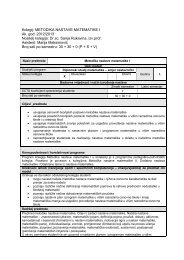
CHAPTER 2Surfaces: Local Theory1. Parametrized Surfaces and the First Fundamental FormLet U be an open set in R 2 .Afunction f : U → R m (for us, m =1and 3 will be most common)is called C 1 if f and its partial derivatives ∂f ∂fand are all continuous. We will ordinarily use∂u ∂v(u, v) ascoordinates in our parameter space, and (x, y, z) ascoordinates in R 3 . Similarly, for anyk ≥ 2, we say f is C k if all its partial derivatives of order up to k exist and are continuous. We say fis smooth if f is C k for every positive integer k. Wewill henceforth assume all our functions are C kfor k ≥ 3. One of the crucial results for differential geometry is that if f is C 2 , then(and similarly for higher-order derivatives).Notation: We will often also use subscripts to indicate partial derivatives, as follows:f uf vf uuf uv =(f u ) v↔↔↔↔∂f∂u∂f∂v∂ 2 f∂u 2∂ 2 f∂v∂u∂2 f∂u∂v =Definition. A regular parametrization of a subset M ⊂ R 3 isa(C 3 ) one-to-one functionx: U → M ⊂ R 3 so that x u × x v ≠ 0∂2 f∂v∂ufor some open set U ⊂ R 2 . 1 A connected subset M ⊂ R 3 is called a surface if each point has aneighborhood that is regularly parametrized.We might consider the curves on M obtained by fixing v = v 0 and varying u, called a u-curve,and obtained by fixing u = u 0 and varying v, called a v-curve; these are depicted in Figure 1.1. Atthe point P = x(u 0 ,v 0 ), we see that x u (u 0 ,v 0 )istangent to the u-curve and x v (u 0 ,v 0 )istangentto the v-curve. We are requiring that these vectors span a plane, whose normal vector is given byx u × x v .Example 1. We give some basic examples of parametrized surfaces. Note that our parametersdo not necessarily range over an open set of values.1 For technical reasons with which we shall not concern ourselves in this course, we should also require that theinverse function x −1 : x(U) → U be continuous.34

§1. Parametrized Surfaces and the First Fundamental Form 35vxx vx u ×x vv-curvex uuu-curveFigure 1.1(a) The graph of a function f : U → R, z = f(x, y), is parametrized by x(u, v) =(u, v, f(u, v)).Note that x u × x v =(−f u , −f v , 1) ≠ 0, sothis is always a regular parametrization.(b) The helicoid, asshown in Figure 1.2, is the surface formed by drawing horizontal rays fromFigure 1.2the axis of the helix α(t) =(cos t, sin t, bt) topoints on the helix:x(u, v) =(u cos v, u sin v, bv), u ≥ 0, v∈ R.Note that x u × x v =(b sin v, −b cos v, u) ≠ 0. The u-curves are rays and the v-curves arehelices.(c) The torus (surface of a doughnut) is formed by rotating a circle of radius b about a circleof radius a > b lying in an orthogonal plane, as pictured in Figure 1.3. The regularparametrization is given byx(u, v) =((a + b cos u) cos v, (a + b cos u) sin v, b sin u), 0 ≤ u, v < 2π.Then x u × x v = −b(a + b cos u) ( cos u cos v, cos u sin v, sin u ) , which is never 0.(d) The standard parametrization of the unit sphere Σ is given by spherical coordinates (φ, θ) ↔(u, v):x(u, v) =(sin u cos v, sin u sin v, cos u),0

36 Chapter 2. Surfaces: Local TheoryavubuFigure 1.3Since x u × x v = sin u(sin u cos v, sin u sin v, cos u) =(sin u)x(u, v), the parametrization isregular away from u =0,π, which we’ve excluded anyhow because x fails to be one-to-oneat such points. The u-curves are the so-called lines of longitude and the v-curves are thelines of latitude on the sphere.(e) Another interesting parametrization of the sphere is given by stereographic projection. (Cf.Exercise 1.1.1.) We parametrize the unit sphere less the north pole (0, 0, 1) by the xy-plane,(0,0,1)(x,y,z)(u,v,0)Figure 1.4assigning to each (u, v) the point (≠ (0, 0, 1)) where the line through (0, 0, 1) and (u, v, 0)intersects the unit sphere, as pictured in Figure 1.4. We leave it to the reader to derive thefollowing formula in Exercise 1:(x(u, v) =2uu 2 + v 2 +1 ,2vu 2 + v 2 +1 , u2 + v 2 )− 1u 2 + v 2 . ▽+1For our last examples, we give two general classes of surfaces that will appear throughout ourwork.

§1. Parametrized Surfaces and the First Fundamental Form 37Example 2. Let I ⊂ R be an interval, and let α(u) =(0,f(u),g(u)), u ∈ I, bearegularparametrized plane curve with f>0. Then the surface of revolution obtained by rotating α aboutthe z-axis is parametrized byx(u, v) = ( f(u) cos v, f(u) sin v, g(u) ) ,u ∈ I, 0 ≤ v

38 Chapter 2. Surfaces: Local Theoryhypothesis, the vectors x u and x v are linearly independent and must therefore span a plane. Wenow make this an officialDefinition. Let M be a regular parametrized surface, and let P ∈ M. Then choose a regularparametrization x: U → M ⊂ R 3 with P = x(u 0 ,v 0 ). We define the tangent plane of M at P tobe the subspace T P M spanned by x u and x v (evaluated at (u 0 ,v 0 )).Remark. The alert reader may wonder what happens if two people pick two different such localparametrizations of M near P .Dothey both provide the same plane T P M? This sort of questionis very common in differential geometry, and is not one we intend to belabor in this introductorycourse. However, to get a feel for how such arguments go, the reader may work Exercise 11.There are two unit vectors orthogonal to the tangent plane T P M. Given a regular parametrizationx, weknow that x u × x v is a nonzero vector orthogonal to the plane spanned by x u and x v ;we obtain the corresponding unit vector by takingn =x u × x v‖x u × x v ‖ .This is called the unit normal of the parametrized surface.Example 4. We know from basic geometry and vector calculus that the unit normal of theunit sphere centered at the origin should be the position vector itself. This is in fact what wediscovered in Example 1(d). ▽Example 5. Consider the helicoid given in Example 1(b). Then, as we saw, x u × x v =1(b sin v, −b cos v, u), and n = √u 2 + b (b sin v, −b cos v, u). As we move along a ruling v = v 0,2the normal starts horizontal at u =0(where the surface becomes vertical) and rotates in the planeorthogonal to the ruling, becoming more and more vertical as we move out the ruling. ▽We saw in Chapter 1 that the geometry of a space curve is best understood by calculating (atleast in principle) with an arclength parametrization. It would be nice, analogously, if we couldfind a parametrization x(u, v) ofasurface so that x u and x v form an orthonormal basis at eachpoint. We’ll see later that this can happen only very rarely. But it makes it natural to introducewhat is classically called the first fundamental form, I P (U, V) =U · V, for U, V ∈ T P M.Workingin a parametrization, we have the natural basis {x u , x v }, and so we defineE =I P (x u , x u )=x u · x uF =I P (x u , x v )=x u · x v = x v · x u =I P (x v , x u )G =I P (x v , x v )=x v · x v ,and it is often convenient to put these in as entries of a (symmetric) matrix:[ ]E FI P = .F GThen, given tangent vectors U = ax u + bx v and V = cx u + dx v ∈ T P M,wehaveU · V =I P (U, V) =(ax u + bx v ) · (cx u + dx v )=E(ac)+F (ad + bc)+G(bd).

§1. Parametrized Surfaces and the First Fundamental Form 39In particular, ‖U‖ 2 =I P (U, U) =Ea 2 +2Fab+ Gb 2 .Suppose M and M ∗ are surfaces. We say they are locally isometric if for each P ∈ M there are aregular parametrization x: U → M with x(u 0 ,v 0 )=P and a regular parametrization x ∗ : U → M ∗(using the same domain U ⊂ R 2 ) with the property that I P =I ∗ P ∗ whenever P = x(u, v) andP ∗ = x ∗ (u, v) for some (u, v) ∈ U. That is, the function f = x ∗ ◦x −1 : x(U) → x ∗ (U) isaone-to-onecorrespondence that preserves the first fundamental form and is therefore distance-preserving (seeExercise 3).Example 6. Parametrize a portion of the plane (say, a piece of paper) by x(u, v) =(u, v, 0) andaportion of a cylinder by x ∗ (u, v) =(cos u, sin u, v). Then it is easy to calculate that E = E ∗ =1,F = F ∗ =0,and G = G ∗ =1,sothese surfaces, pictured in Figure 1.6, are locally isometric. OnfoldsealFigure 1.6the other hand, if we let u vary from 0 to 2π, the rectangle and the cylinder are not globally isometricbecause points far away in the rectangle can become very close (or identical) in the cylinder. ▽If α(t) =x(u(t),v(t)) is a curve on the parametrized surface M with α(t 0 )=x(u 0 ,v 0 )=P ,then it is an immediate consequence of the chain rule, Theorem 2.2 of the Appendix, thatα ′ (t 0 )=u ′ (t 0 )x u (u 0 ,v 0 )+v ′ (t 0 )x v (u 0 ,v 0 ).(Customarily we will write simply x u , the point (u 0 ,v 0 )atwhich it is evaluated being assumed.)That is, if the tangent vector (u ′ (t 0 ),v ′ (t 0 )) back in the “parameter space” is (a, b), then the tangentvector to α at P is the corresponding linear combination ax u + bx v .Infancy terms, this is merelya consequence of the linearity of the derivative of x. Wesayaparametrization x(u, v) isconformal(a,b)xPx v(u 0 ,v 0 )x uax u + bx vFigure 1.7

40 Chapter 2. Surfaces: Local Theoryif angles measured in the uv-plane agree with corresponding angles in T P M for all P .Weleave itto the reader to check in Exercise 5 that this is equivalent to the conditions E = G, F =0.Sincewe have[EF]F=G[]x u · x u x u · x vx v · x u x v · x v⎡| |⎢= ⎣ x u x v| |⎤⎥⎦T ⎡| |⎢⎣ x u x v| |⎛⎡⎤⎞([]) x u · x u x u · x v 0EG − F 2 x u · x u x u · x v ⎜⎢⎥⎟= det= det ⎝⎣x v · x u x v · x v 0 ⎦⎠x v · x u x v · x v0 0 1⎛⎡⎤T ⎡ ⎤⎞⎛ ⎡ ⎤⎞| | | | | || | |= det ⎜⎢⎥ ⎢ ⎥⎝⎣x u x v n ⎦ ⎣ x u x v n ⎦⎟⎠ = ⎜ ⎢ ⎥⎟⎝det ⎣ x u x v n ⎦⎠| | | | | || | |which is the square of the volume of the parallelepiped spanned by x u , x v , and n. Since n is a unitvector orthogonal to the plane spanned by x u and x v , this is, in turn, the square of the area of theparallelogram spanned by x u and x v . That is,EG − F 2 = ‖x u × x v ‖ 2 ≠0.We remind the reader that we obtain the surface area of the parametrized surface x: U → M bycalculating the double integral∫∫ √‖x u × x v ‖dudv = EG − F 2 dudv.UU⎤⎥⎦ ,2,EXERCISES 2.11. Derive the formula given in Example 1(e) for the parametrization of the unit sphere.2. Compute I (i.e., E, F , and G) for the following parametrized surfaces.*a. the sphere of radius a: x(u, v) =a(sin u cos v, sin u sin v, cos u)b. the torus: x(u, v) =((a + b cos u) cos v, (a + b cos u) sin v, b sin u) (0

§1. Parametrized Surfaces and the First Fundamental Form 41*4. Show that if all the normal lines to a surface pass through a fixed point, then the surface is (aportion of) a sphere. (By the normal line to M at P we mean the line passing through P withdirection vector the unit normal at P .)5. Check that the parametrization x(u, v) isconformal if and only if E = G and F =0. (Hint:For =⇒, choose two convenient pairs of orthogonal directions.)*6. Check that the parametrization of the unit sphere by stereographic projection (see Example1(e)) is conformal.7. Consider the hyperboloid of one sheet, M, given by the equation x 2 + y 2 − z 2 =1.a. Show that x(u, v) =(cosh u cos v, cosh u sin v, sinh u) gives a parametrization of M as asurface of revolution.*b. Find two parametrizations ( of M as a ruled surface α(u)+vβ(u).uv +1c. Show that x(u, v) =uv − 1 , u − vuv − 1 , u + v )gives a parametrization of M where bothuv − 1sets of parameter curves are rulings.♯ 8.Given a ruled surface x(u, v) =α(u)+vβ(u) with α ′ ≠0and ‖β‖ =1;suppose that α ′ (u),β(u), and β ′ (u) are linearly dependent for every u. Prove that locally one of the following musthold:(i) β = const;(ii) there is a function λ so that α(u)+λ(u)β(u) =const;(iii) there is a function λ so that (α + λβ) ′ (u) isanonzero multiple of β(u) for every u.Describe the surface in each of these cases. (Hint: There are c 1 , c 2 , c 3 (functions of u), neversimultaneously 0, so that c 1 (u)α ′ (u)+c 2 (u)β(u)+c 3 (u)β ′ (u) =0 for all u. Consider separatelythe cases c 1 (u) =0and c 1 (u) ≠0.Inthe latter case, divide through.)9. (The Mercator projection) Mercator developed his system for mapping the earth, as pictured inuvFigure 1.8Figure 1.8, in 1569, about a century before the advent of calculus. We want a parametrizationx(u, v) ofthe sphere, u ∈ R, v ∈ [0, 2π), so that the u-curves are the longitudes and sothat the parametrization is conformal. Letting (φ, θ) bethe usual spherical coordinates, write

42 Chapter 2. Surfaces: Local Theoryφ = f(u) and θ = v. Show that conformality and symmetry about the equator will dictatef(u) =2arctan(e −u ). Deduce that(Cf. Example 2 in Section 1 of Chapter 1.)x(u, v) =(sechu cos v, sechu sin v, tanh u).10. A parametrization x(u, v) iscalled a Tschebyschev net if the opposite sides of any quadrilateralformed by the coordinate curves have equal length.a. Prove that this occurs if and only if ∂E∂v = ∂G =0. (Hint: Express the length of the∂uu-curves, u 0 ≤ u ≤ u 1 ,asanintegral and use the fact that this length is independent ofv.)b. Prove that we can locally reparametrize by ˜x(ũ, ṽ) soastoobtain Ẽ = ˜G =1, ˜F =cos θ(ũ, ṽ) (so that the ũ- and ṽ-curves are parametrized by arclength and meet at angle/θ). (Hint: Choose ũ as a function of u so that ˜xũ = x u (dũ/du) has unit length.)11. Suppose x and y are two parametrizations of a surface M near P .Sayx(u 0 ,v 0 )=P = y(s 0 ,t 0 ).Prove that Span(x u , x v )=Span(y s , y t ) (where the partial derivatives are all evaluated at theobvious points). (Hint: f = x −1 ◦y gives a C 1 map from an open set around (s 0 ,t 0 )toanopenset around (u 0 ,v 0 ). Apply the chain rule to show y s , y t ∈ Span(x u , x v ).)12. (A programmable calculator or Maple may be useful for parts of this problem.) A catenoid, aspictured in Figure 1.9, is parametrized byx(u, v) =(a cosh u cos v, a cosh u sin v, au), u ∈ R, 0 ≤ v0 fixed).Figure 1.9*a. Compute the surface area of that portion of the catenoid given by |u| ≤ 1/a. (Hint:cosh 2 u = 1 2(1 + cosh 2u).)b. Given the pair of parallel circles x 2 + y 2 = R 2 , |z| =1,for what values of R is there atleast one catenoid with the circles as boundary? (Hint: Graph f(t) =t cosh(1/t).)c. For the values of R in part b, compare the area of the catenoid(s) with 2πR 2 , the area ofthe pair of disks filling in the circles. For what values of R does the pair of disks have theleast area?13. There are two obvious families of circles on a torus. Find a third family. (Hint: Look for a planethat is tangent to the torus at two points. Using the parametrization of the torus, you should

§2. The Gauss Map and the Second Fundamental Form 43be able to find parametric equations for the curve in which the bitangent plane intersects thetorus.)2. The Gauss Map and the Second Fundamental FormGiven a regular parametrized surface M, the function n: M → Σ that assigns to each pointP ∈ M the unit normal n(P ), as pictured in Figure 2.1, is called the Gauss map of M. Asweshallsee in this chapter, most of the geometric information about our surface M is encapsulated in thePnn(P)Figure 2.1mapping n.Example 1. A few basic examples are these.(a) On a plane, the tangent plane never changes, so the Gauss map is a constant.(b) On a cylinder, the tangent plane is constant along the rulings, so the Gauss map sends theentire surface to an equator of the sphere.(c) On a sphere centered at the origin, the Gauss map is merely the (normalized) positionvector.(d) On a saddle surface (as pictured in Figure 2.1), the Gauss map appears to “reverse orientation”:As we move counterclockwise in a small circle around P ,wesee that the unit vectorn turns clockwise around n(P ). ▽Recall from the Appendix that for any function f on M (scalar- or vector-valued) and anytangent vector V ∈ T P M,wecan compute the directional derivative D V f(P )bychoosing a curveα: (−ε, ε) → M with α(0) = P and α ′ (0) = V and computing (f ◦α) ′ (0).To understand the shape of M at the point P , might try to understand the curvature at P ofvarious curves in M. Perhaps the most obvious thing to try is various normal slices of M. That is,we slice M with the plane through P spanned by n(P ) and a unit vector V ∈ T P M.Various suchnormal slices are shown for a saddle surface in Figure 2.2. Let α be the arclength-parametrizedcurve obtained by taking such a normal slice. We have α(0) = P and α ′ (0) = V. Then since thecurve lies the plane spanned by n(P ) and V, the principal normal of the curve at P must be ±n(P )(+ if the curve is curving towards n, − if it’s curving away). Applying Lemma 2.1 of Chapter 1

44 Chapter 2. Surfaces: Local TheoryFigure 2.2yet again, we have:(†)±κ = κN · n = T ′ (0) · n = −T · (n◦α) ′ (0) = −D V n(P ) · V.This leads us to study the directional derivative D V n(P ) more carefully.Proposition 2.1. For any V ∈ T P M, the directional derivative D V n(P ) ∈ T P M. Moreover,the linear map S P : T P M → T P M defined byS P (V) =−D V n(P )is a symmetric linear map; i.e., for any U, V ∈ T P M,wehave(∗)S P (U) · V = U · S P (V)S P is called the shape operator at P .Proof. Forany curve α: (−ε, ε) → M with α(0) = P and α ′ (0) = V, weobserve that n◦α hasconstant length 1. Thus, by Lemma 2.1 of Chapter 1, D V n(P )·n(P )=(n◦α) ′ (0)·(n◦α)(0) = 0, soD V n(P )isinthe tangent plane to M at P . That S P is a linear map is an immediate consequenceof Proposition 2.3 of the Appendix.Symmetry is our first important application of the equality of mixed partial derivatives. Firstwe verify (∗) when U = x u , V = x v . Note that n · x v =0,so0= ( n · x v)u = n u · x v + n · x vu .(Remember that we’re writing n u for D xu n.) Thus,S P (x u ) · x v = −D xu n(P ) · x v = −n u · x v = n · x vu= n · x uv = −n v · x u = −D xv n(P ) · x u = S P (x v ) · x u .

§2. The Gauss Map and the Second Fundamental Form 45Next, knowing this, we just write out general vectors U and V as linear combinations of x u andx v :IfU = ax u + bx v and V = cx u + dx v , thenS P (U) · V = S P (ax u + bx v ) · (cx u + dx v )= ( aS P (x u )+bS P (x v ) ) · (cx u + dx v )= acS P (x u ) · x u + adS P (x u ) · x v + bcS P (x v ) · x u + bdS P (x v ) · x v= acS P (x u ) · x u + adS P (x v ) · x u + bcS P (x u ) · x v + bdS P (x v ) · x v=(ax u + bx v ) · (cSP (x u )+dS P (x v ) ) = U · S P (V),as required.□Proposition 2.2. If the shape operator S P is O for all P ∈ M, then M is a subset of a plane.Proof. Since the directional derivative of the unit normal n is 0 in every direction at everypoint P ,wehaven u = n v = 0 for any (local) parametrization x(u, v) ofM. ByProposition 2.4 ofthe Appendix, it follows that n is constant. (This is why we assume our surfaces are connected.) □Example 2. Let M be a sphere of radius a centered at the origin. Then n = 1 x(u, v), so foraany P ,wehaveS P (x u )=−n u = − 1 a x u and S P (x v )=−n v = − 1 a x v,soS Pidentity map on each tangent plane. ▽is −1/a times theIt does not seem an easy task to give the matrix of the shape operator with respect to thebasis {x u , x v }. But, in general, the proof of Proposition 2.1 suggests that we define the secondfundamental form, as follows. If U, V ∈ T P M,wesetII P (U, V) =S P (U) · V.Note that the formula (†) onp.44shows that the curvature of the normal slice in direction V (with‖V‖ =1)is, in our new notation, given by±κ = −D V n(P ) · V = S P (V) · V =II P (V, V).As we did at the end of the previous section, we wish to give a matrix representation whenwe’re working with a parametrized surface. As we saw in the proof of Proposition 2.1, we havel =II P (x u , x u )= −D xu n · x u = x uu · nm =II P (x u , x v )= −D xu n · x v = x vu · n = x uv · n =II P (x v , x u )n =II P (x v , x v )=−D xv n · x v = x vv · n.(By the way, this explains the presence of the minus sign in the original definition of the shapeoperator.) We then write[ ] []l m x uu · n x uv · nII P = =.m n x uv · n x vv · nIf, as before, U = ax u + bx v and V = cx u + dx v , thenII P (U, V) =II P (ax u + bx v ,cx u + dx v )= acII P (x u , x u )+adII P (x u , x v )+bcII P (x v , x u )+bdII P (x v , x v )

46 Chapter 2. Surfaces: Local Theory= l(ac)+m(bc + ad)+n(bd).In the event that {x u , x v } is an orthonormal basis for T P M,wesee that the matrix II P representsthe shape operator S P . But it is not difficult to check (see Exercise 2) that, in general, the matrixof the linear map S P with respect to the basis {x u , x v } is given byI −1P II P =[EF] −1 [F lG m]m.nRemark. We proved in Proposition 2.1 that S P is a symmetric linear map. This means thatits matrix representation with respect to an orthonormal basis (or, more generally, orthogonal basiswith vectors of equal length) will be symmetric: In this case the matrix I P is a scalar multiple ofthe identity matrix and the matrix product remains symmetric.By the Spectral Theorem, Theorem 1.3 of the Appendix, S P has two real eigenvalues, traditionallydenoted k 1 (P ), k 2 (P ).Definition. The eigenvalues of S P are called the principal curvatures of M at P . Correspondingeigenvectors are called principal directions. A curve in M is called a line of curvature if itstangent vector at each point is a principal direction.Recall that it also follows from the Spectral Theorem that the principal directions are orthogonal,so we can always choose an orthonormal basis for T P M consisting of principal directions. Havingdone so, we can then easily determine the curvatures of normal slices in arbitrary directions, asfollows.Proposition 2.3 (Euler’s Formula). Let e 1 , e 2 be unit vectors in the principal directions atP with corresponding principal curvatures k 1 and k 2 . Suppose V = cos θe 1 + sin θe 2 for someθ ∈ [0, 2π), aspictured in Figure 2.3. Then II P (V, V) =k 1 cos 2 θ + k 2 sin 2 θ.e 2Vθ e 1Figure 2.3Proof. This is a straightforward computation: Since S P (e i )=k i e i for i =1, 2, we haveII P (V, V) =S P (V) · V = S P (cos θe 1 + sin θe 2 ) · (cos θe 1 + sin θe 2 )= (cos θk 1 e 1 + sin θk 2 e 2 ) · (cos θe 1 + sin θe 2 )=k 1 cos 2 θ + k 2 sin 2 θ,as required.□

§2. The Gauss Map and the Second Fundamental Form 47On a sphere, all normal slices have the same (nonzero) curvature. On the other hand, if we lookcarefully at Figure 2.2, we see that certain normal slices of a saddle surface are true lines. Thisleads us to make the followingDefinition. If the normal slice in direction V has zero curvature, i.e., if II P (V, V) =0, thenwe call V an asymptotic direction. 2 A curve in M is called an asymptotic curve if its tangent vectorat each point is an asymptotic direction.Example 3. If a surface M contains a line, that line is an asymptotic curve. For the normalslice in the direction of the line contains the line (and perhaps other things far away), which, ofcourse, has zero curvature. ▽Corollary 2.4. There is an asymptotic direction at P if and only if k 1 k 2 ≤ 0.Proof. k 2 =0if and only if e 2 is an asymptotic direction. Now suppose k 2 ≠0. IfV isa unit asymptotic vector making angle θ with e 1 , then we have k 1 cos 2 θ + k 2 sin 2 θ =0,and sotan 2 θ = −k 1 /k 2 ,sok 1 k 2 ≤ 0. Conversely, if k 1 k 2 ≤ 0, take θ with tan θ = ± √ −k 1 /k 2 , and thenV is an asymptotic direction. □Example 4. We consider the helicoid, as pictured in Figure 1.2. It is a ruled surface and sothe rulings are asymptotic curves. What is quite less obvious is that the family of helices on thesurface are also asymptotic curves. But, as we see in Figure 2.4, the normal slice tangent to thePFigure 2.4helix at P has an inflection point at P , and therefore the helix is an asymptotic curve. We ask thereader to check this by calculation in Exercise 5. ▽It is also an immediate consequence of Proposition 2.3 that the principal curvatures are themaximum and minimum (signed) curvatures of the various normal slices. Assume k 2 ≤ k 1 . Thenk 1 cos 2 θ + k 2 sin 2 θ = k 1 (1 − sin 2 θ)+k 2 sin 2 θ = k 1 +(k 2 − k 1 ) sin 2 θ ≤ k 12 Of course, V ̸=0 here. See Exercise 21 for an explanation of this terminology.

48 Chapter 2. Surfaces: Local Theory(and, similarly, ≥ k 2 ). Moreover, as the Spectral Theorem tells us, the maximum and minimumoccur at right angles to one another. Looking back at Figure 2.2, where the slices are taken at anglesin increments of π/8, we see that the normal slices that are “most curved” appear in the third andseventh frames; the asymptotic directions appear in the second and fourth frames. (Cf. Exercise8.)Next we come to one of the most important concepts in the geometry of surfaces:Definition. The product of the principal curvatures is called the Gaussian curvature: K =det S P = k 1 k 2 . The average of the principal curvatures is called the mean curvature: H = 1 2 trS P =12 (k 1 + k 2 ). We say M is a minimal surface if H =0.Note that whereas the signs of the principal curvatures change if we reverse the direction of theunit normal n, the Gaussian curvature K, being the product of both, is independent of the choiceof unit normal. (And the sign of the mean curvature depends on the choice.)Definition. Fix P ∈ M. We say P is an umbilic 3 if k 1 = k 2 . If k 1 = k 2 =0,wesayP is aplanar point. IfK =0but P is not a planar point, we say P is a parabolic point. IfK>0, we sayP is an elliptic point, and if K

§2. The Gauss Map and the Second Fundamental Form 49rectangle collapses to a line segment; for a saddle surface, orientation is reversed by n and so theGaussian curvature is negative.)Let’s close this section by revisiting our discussion of the curvature of normal slices. Suppose αis an arclength-parametrized curve lying on M with α(0) = P and α ′ (0) = V. Then the calculationin formula (†) onp.44shows thatII P (V, V) =κN · n;i.e., II P (V, V) gives the component of the curvature vector κN of α normal to the surface M atP , which we denote by κ n and call the normal curvature of α at P . What is remarkable aboutthis formula is that it shows that the normal curvature depends only on the direction of α at Pand otherwise not on the curve. (For the case of the normal slice, the normal curvature is, up to asign, all the curvature.) We immediately deduce the followingProposition 2.5 (Meusnier’s Formula). Let α be acurve on M passing through P with unittangent vector V. ThenII P (V, V) =κ n = κ cos φ,where φ is the angle between the principal normal, N, ofα and the surface normal, n, atP .In particular, if α is an asymptotic curve, then its normal curvature is 0 at each point.Example 6. Let’s now investigate a very interesting surface, called the pseudosphere, asshownin Figure 2.6. It is the surface of revolution obtained by rotating the tractrix (see Example 2 ofnNFigure 2.6Chapter 1, Section 1) about the x-axis, and so it is parametrized byx(u, v) =(u − tanh u, sechu cos v, sechu sin v),u > 0, v∈ [0, 2π).Note that the circles (of revolution) are lines of curvature: Either apply Exercise 13 or observe,directly, that the only component of the surface normal that changes as we move around the circle isnormal to the circle in the plane of the circle. Similarly, the various tractrices are lines of curvature:In the plane of one tractrix, the surface normal and the curve normal agree.Now, by Exercise 1.2.5, the curvature of the tractrix is κ =1/ sinh u; since N = n along thiscurve, we have k 1 = κ n =1/ sinh u. Now what about the circles? Here we have κ =1/sechu =cosh u, but this is not the normal curvature. The angle θ we see in Figure 1.9 of Chapter 1 isthe same as the angle φ between N and n in Figure 2.6 (to see why, see Figure 2.7). Thus, by

50 Chapter 2. Surfaces: Local TheorynN1tanh uθFigure 2.7Meusnier’s Formula, Proposition 2.5, we have k 2 = κ n = κ cos φ = (cosh u)(− tanh u) =− sinh u.Amazingly, then, we have K = k 1 k 2 =(1/ sinh u)(− sinh u) =−1. ▽Example 7. Let’s now consider the case of a general surface of revolution, parametrized as inExample 2 of Section 1, byx(u, v) = ( f(u) cos v, f(u) sin v, g(u) ) ,where f ′ (u) 2 +g ′ (u) 2 =1. Recall that the u-curves are called meridians and the v-curves are calledparallels. Thenand so we havex u = ( f ′ (u) cos v, f ′ (u) sin v, g ′ (u) )x v = ( −f(u) sin v, f(u) cos v, 0 )n = ( −g ′ (u) cos v, −g ′ (u) sin v, f ′ (u) )x uu = ( f ′′ (u) cos v, f ′′ (u) sin v, g ′′ (u) )x uv = ( −f ′ (u) sin v, f ′ (u) cos v, 0 )x vv = ( −f(u) cos v, −f(u) sin v, 0 ) ,E =1, F =0, G = f(u) 2 and l = f ′ (u)g ′′ (u) − f ′′ (u)g ′ (u), m =0, n = f(u)g ′ (u).By Exercise 2.2.1, then k 1 = f ′ (u)g ′′ (u) − f ′′ (u)g ′ (u) and k 2 = g ′ (u)/f(u). Thus,K = k 1 k 2 = ( f ′ (u)g ′′ (u) − f ′′ (u)g ′ (u) ) g ′ (u)f(u) = −f′′ (u)f(u) ,since from f ′ (u) 2 + g ′ (u) 2 =1we deduce that f ′ (u)f ′′ (u)+g ′ (u)g ′′ (u) =0,and sof ′ (u)g ′ (u)g ′′ (u) − f ′′ (u)g ′ (u) 2 = −(f ′ (u) 2 + g ′ (u) 2 )f ′′ (u) =−f ′′ (u).Note, as we observed in the special case of Example 6, that on every surface of revolution, themeridians and the parallels are lines of curvature. ▽

§2. The Gauss Map and the Second Fundamental Form 51EXERCISES 2.2*1. Check that the parameter curves are lines of curvature if and only if F = m =0. Show,moreover, that in this event, we have the principal curvatures k 1 = l/E and k 2 = n/G.♯ 2. a. Show that the matrix representing the linear map S P : T P M → T P M with respect to thebasis {x u , x v } isI −1P II P =[EF] −1 [F lG m]m.n(Hint: It suffices to check S P (x u ) · x u , S P (x u ) · x v , and so on.)ln − m2b. Deduce that K =EG − F 2 .3. Compute the second fundamental form II P of the following parametrized surfaces. Then calculatethe matrix of the shape operator, determine H and K.a. the cylinder: x(u, v) =(a cos u, a sin u, v)*b. the torus: x(u, v) =((a + b cos u) cos v, (a + b cos u) sin v, b sin u) (0

52 Chapter 2. Surfaces: Local Theoryc. (More challenging) Show that, more generally, for any θ and m ≥ 3, we haveH = 1 (( 2π ) ( 2π(m − 1) ) )κ n (θ)+κ n θ + + ···+ κn θ + .mmm10. a. Apply Meusnier’s Formula to a latitude circle on a sphere of radius a to calculate thenormal curvature.b. Prove that the curvature of any curve lying on the sphere of radius a satisfies κ ≥ 1/a.11. Prove or give a counterexample: If M is a surface with Gaussian curvature K>0, then thecurvature of any curve C ⊂ M is everywhere positive. (Remember that, by definition, κ ≥ 0.)♯ 12.Suppose that for every P ∈ M, the shape operator S P is some scalar multiple of the identity,i.e., S P (V) =k(P )V for all V ∈ T P M. (Here the scalar k(P )maywell depend on the pointP .)a. Differentiate the equationsD xu n = n u = − kx uD xv n = n v = − kx vappropriately to determine k u and k v and deduce that k must be constant.b. We showed in Proposition 2.2 that M is planar when k =0. Show that when k ≠0,M is(a portion of) a sphere.13. a. Prove that if α is a line of curvature in M, then (n◦α) ′ (t) =−k(t)α ′ (t), where k(t) istheprincipal curvature at α(t) inthe direction α ′ (t). (More colloquially, differentiating alongthe curve α, wejust write n ′ = −kα ′ .)b. Suppose two surfaces M and M ∗ intersect along a curve C. Suppose C is a line of curvaturein M. Prove that C is a line of curvature in M ∗ if and only if the angle between M andM ∗ is constant along C. (In the proof of ⇐=, be sure to include the case that M and M ∗intersect tangentially along C.)14. Prove or give a counterexample:a. If a curve is both an asymptotic curve and a line of curvature, then it must be planar.b. If a curve is planar and an asymptotic curve, then it must be a line.15. a. How is the Frenet frame along an asymptotic curve related to the geometry of the surface?b. Suppose K(P ) < 0. If C is an asymptotic curve with κ(P ) ≠0,prove that its torsionsatisfies |τ(P )| = √ −K(P ). (Hint: If we choose an orthonormal basis {U, V} for T P (M)with U tangent to C, what is the matrix for S P ? See the Remark on p. 46.)16. Continuing Exercise 15, show that if K(P ) < 0, then the two asymptotic curves have torsionof opposite signs at P .17. Prove that the only minimal ruled surface with no planar points is the helicoid. (Hint: Considerthe curves orthogonal to the rulings. Use Exercises 8b and 1.2.19.)

§2. The Gauss Map and the Second Fundamental Form 5318. Suppose U ⊂ R 3 is open and x: U → R 3 is a smooth map (of rank 3) so that x u , x v , and x ware always orthogonal. Then the level surfaces u = const, v = const, w = const form a triplyorthogonal system of surfaces.a. Show that the spherical coordinate mapping x(u, v, w) =(u sin v cos w, u sin v sin w, u cos v)furnishes an example.b. Prove that the curves of intersection of any pair of surfaces from different systems (e.g.,v = const and w = const) are lines of curvature in each of the respective surfaces. (Hint:Differentiate the various equations x u · x v =0,x v · x w =0,x u · x w =0with respect to themissing variable. What are the shape operators of the various surfaces?)19. In this exercise we analyze the surfaces of revolution that are minimal. It will be convenient towork with a meridian as a graph (y = h(u), z = u), as opposed to our customary parametrizationof surfaces of revolution.a. Use Exercise 1.2.4 and Proposition 2.5 to show that the principal curvatures arek 1 =h ′′(1 + h ′2 ) 3/2 and k 2 = − 1 h · 1√ .1+h ′2b. Deduce that H =0if and only if h(u)h ′′ (u) =1+h ′ (u) 2 .c. Solve the differential equation. (Hint: Either substitute z(u) =lnh(u)orintroduce w(u) =h ′ (u), find dw/dh, and integrate by separating variables.) You should find that h(u) =1ccosh(cu + b) for some constants b and c.20. By choosing coordinates in R 3 appropriately, we may arrange that P is the origin, the tangentplane T P M is the xy-plane, and the x- and y-axes are in the principal directions at P .a. Show that in these coordinates M is locally the graph z = f(x, y) = 1 2 (k 1x 2 + k 2 y 2 )+...,...where limx,y→0 x 2 + y 2 =0.(Youmay start with Taylor’s Theorem: if f is C2 ,wehavewheref(x, y) =f(0, 0) + f x (0, 0)x + f y (0, 0)y +limx,y→0...x 2 + y 2 = 0.)12(fxx (0, 0)x 2 +2f xy (0, 0)xy + f yy (0, 0)y 2) + ...,b. Show that if P is an elliptic point, then a neighborhood of P in M ∩ T P M is just theorigin itself. Show that if P is a hyperbolic point, such a neighborhood is a curve thatcrosses itself at P and whose tangent directions at P are the asymptotic directions. Whathappens in the case of a parabolic point?21. Let P ∈ M be a non-planar point, and if K ≥ 0, choose the unit normal so that l, n ≥ 0.a. We define the Dupin indicatrix to be the conic in T P M defined by the equation II P (V, V) =1. Show that if P is an elliptic point, the Dupin indicatrix is an ellipse; if P is a hyperbolicpoint, the Dupin indicatrix is a hyperbola; and if P is a parabolic point, the Dupinindicatrix is a pair of parallel lines.b. Show that if P is a hyperbolic point, the asymptotes of the Dupin indicatrix are given byII P (V, V) =0, i.e., the set of asymptotic directions.

54 Chapter 2. Surfaces: Local Theoryc. Suppose M is represented locally near P as in Exercise 20. Show that for small positivevalues of c, the intersection of M with the plane z = c “looks like” the Dupin indicatrix.How can you make this statement more precise?22. Suppose the surface M is given near P as a level surface of a smooth function f : R 3 → R with∇f(P ) ≠0.Aline L ⊂ R 3 is said to have (at least) k-point contact with M at P if, given anylinear parametrization α of L with α(0) = P , the function f = f ◦α vanishes to order k − 1,i.e., f(0) = f ′ (0) = ···= f (k−1) (0) = 0. (Such a line is to be visualized as the limit of lines thatintersect M at P and at k − 1 other points that approach P .)a. Show that L has 2-point contact with M at P if and only if L is tangent to M at P , i.e.,L ⊂ T P M.b. Show that L has 3-point contact with M at P if and only if L is an asymptotic directionat P . (Hint: It may be helpful to follow the setup of Exercise 20.)c. (Challenge) What does it mean for L to have 4-point contact with M at P ?3. The Codazzi and Gauss Equations and the Fundamental Theorem of SurfaceTheoryWe now wish to proceed towards a deeper understanding of Gaussian curvature. We have tothis point considered only the normal components of the second derivatives x uu , x uv , and x vv .Nowlet’s consider them in toto. Since {x u , x v , n} gives a basis for R 3 , there are functions Γuu, u Γuu,vΓuv u =Γvu, u Γuv v =Γvu, v Γvv, u and Γvv v so that(†)x uu =Γ u uux u +Γ v uux v + lnx uv =Γ u uvx u +Γ v uvx v + mnx vv =Γ uvvx u +Γ vvvx v + nn.(Note that x uv = x vu dictates the symmetries Γ uv • =Γ vu.) • The functions Γ •• • are called Christoffelsymbols.Example 1. Let’s compute the Christoffel symbols for the usual parametrization of the sphere.By straightforward calculation we obtainx u = (cos u cos v, cos u sin v, − sin u)x v =(− sin u sin v, sin u cos v, 0)x uu =(− sin u cos v, − sin u sin v, − cos u) =−x(u, v)x uv =(− cos u sin v, cos u cos v, 0)x vv =(− sin u cos v, − sin u sin v, 0) = − sin u(cos v, sin v, 0).(Note that the u-curves are great circles, parametrized by arclength, so it is no surprise that theacceleration vector x uu is inward-pointing of length 1. The v-curves are latitude circles of radiussin u, so, similarly, the acceleration vector x vv points inwards towards the center of the respectivecircle.)

§3. The Codazzi and Gauss Equations and the Fundamental Theorem of Surface Theory 55Since x uu lies entirely in the direction of n, wehave Γuu u =Γuu v =0. Now, byinspection,x uv = cot ux v ,soΓuv u =0and Γuv v = cot u. Last, as we can see in Figure 3.1, we have x vv =nx vvsin u cos uusin uux uFigure 3.1− sin u cos ux u − sin 2 un, soΓ uvv = − sin u cos u and Γ vvv =0.▽Now, dotting the equations in (†) with x u and x v givesx uu · x u =ΓuuE u +ΓuuFvx uu · x v =ΓuuF u +ΓuuGvx uv · x u =ΓuvE u +ΓuvFvx uv · x v =ΓuvF u +ΓuvGvNow observe thatx vv · x u =Γ uvvE +Γ vvvFx vv · x v =Γ uvvF +Γ vvvG.x uu · x u = 1 2 (x u · x u ) u = 1 2 E ux uv · x u = 1 2 (x u · x u ) v = 1 2 E vx uv · x v = 1 2 (x v · x v ) u = 1 2 G ux uu · x v =(x u · x v ) u − x u · x uv = F u − 1 2 E vx vv · x u =(x u · x v ) v − x uv · x v = F v − 1 2 G ux vv · x v = 1 2 (x v · x v ) v = 1 2 G vThus, we can rewrite our equations as follows:[ ][ ] [ ]E F Γuuu 1F G Γuuv =2 E uF u − 1 2 E =⇒v[ ][ ] [ ]E F Γuvu 1F G Γuvv =2 E v(‡)12 G =⇒u[ ][ ] [ ]E F Γvvu F v − 1F G Γvvv =2 G u12 G =⇒v[Γ u uuΓ v uu[Γ u uvΓ v uv[Γ uvvΓ vvv]=[E=F] [E=F] [EF] −1 [ ]1F2 E uG F u − 1 2 E v] −1 [ ]F 12 E v1G2 G u] −1 [ ]F F v − 1 2 G u1G2 G .v

56 Chapter 2. Surfaces: Local TheoryWhat is quite remarkable about these formulas is that the Christoffel symbols, which tell us aboutthe tangential component of the second derivatives x •• , can be computed just from knowing E, F ,and G, i.e., the first fundamental form.Example 2. Let’s now recompute the Christoffel symbols of the unit sphere and compare ouranswers with Example 1. Since E =1,F =0,and G = sin 2 u,wehave[ ] [ ][ ] [ ]Γuuu 1 0 0 0Γuuv =0 csc 2 =u 0 0[ ] [ ][ ] [ ]Γuvu 1 0 00Γuvv =0 csc 2 =u sin u cos u cot u[ ] [ ][] []Γvvu 1 0 − sin u cos u − sin u cos uΓvvv =0 csc 2 =.u 00Thus, the only nonzero Christoffel symbols are Γuv v =Γvu v = cot u and Γvv u = − sin u cos u, asbefore.▽By Exercise 2.2.2, the matrix of the shape operator S P with respect to the basis {x u , x v } is[ ] [ ] −1 [ ][]a c E F l m 1 lG − mF mG − nF==b d F G m n EG − F 2 .−lF + mE −mF + nENote that these coefficients tell us the derivatives of n with respect to u and v:(††)n u = D xu n = −S P (x u )=−(ax u + bx v )n v = D xv n = −S P (x v )=−(cx u + dx v ).We now differentiate the equations (†) again and use equality of mixed partial derivatives. Tostart, we havex uuv =(Γuu) u v x u +Γuux u uv +(Γuu) v v x v +Γuux v vv + l v n + ln v=(Γuu) u v x u +Γuu( u Γuuv x u +Γuvx v v + mn ) +(Γuu) v v x v +Γuuv (Γuvv x u +Γvvx v v + nn)+ l v n − l(cx u + dx v )= ( (Γuu) u v +ΓuuΓ u uv u +ΓuuΓ v vv u − lc ) x u + ( (Γuu) v v +ΓuuΓ u uv v +ΓuuΓ v vv v − ld ) x v+ ( Γuum u +Γuun v )+ l v n,and, similarly,x uvu = ( (Γ u uv) u +Γ u uvΓ u uu +Γ v uvΓ u uv − ma ) x u + ( (Γ v uv) u +Γ u uvΓ v uu +Γ v uvΓ v uv − mb ) x v+ ( lΓ u uv + mΓ v uv + m u)n.Since x uuv = x uvu ,wecompare the indicated components and obtain:(x u ): (Γuu) u v +ΓuuΓ v vv u − lc =(Γuv) u u +ΓuvΓ v uv u − ma(♦) (x v ): (Γuu) v v +ΓuuΓ u uv v +ΓuuΓ v vv v − ld =(Γuv) v u +ΓuvΓ u uu v +ΓuvΓ v uv v − mb(n): l v + mΓuu u + nΓuu v = m u + lΓuv u + mΓuv.v

§3. The Codazzi and Gauss Equations and the Fundamental Theorem of Surface Theory 57Analogously, comparing the indicated components of x uvv = x vvu ,wefind:(x u ): (Γuv) u v +ΓuvΓ u uv u +ΓuvΓ v vv u − mc =(Γvv) u u +Γ u(x v ): (Γuv) v v +ΓuvΓ u uv v − md =(Γvv) v u +ΓvvΓ uuu v − nb(n): m v + mΓuv u + nΓuv v = n u + lΓvv u + mΓvv.vThe two equations coming from the normal component give us theCodazzi equationsvvΓ u uu +Γ vvvΓ u uv − nal v − m u = lΓ u uv + m ( Γ v uv − Γ u uu)− nΓvuum v − n u = lΓ uvv + m ( Γ vvv − Γ u uv)− nΓvuv .ln − m2Using K =EG − F 2 and the formulas above for a, b, c, and d, the four equations involving the x uand x v components yield theGauss equationsEK = ( Γuuv )v − ( Γuvv )u +Γu uuΓuv v +ΓuuΓ v vFK = ( Γuvu )u − ( Γuuu )v +Γv uvΓuv u − ΓuuΓ v vvuFK = ( Γuvv )v − ( Γvvv )u +Γu uvΓuv v − ΓvvΓ uuuvGK = ( Γ uvv)u − ( Γ u uv)v +Γu vvΓ u uu +Γ vvvΓ u uv − ( Γ u uvFor example, to derive the first, we use the equation (♦) above:(Γvuu)v − ( Γ v uvvv − Γ u uvΓ v uu − ( Γ v uv)u +Γu uuΓ v uv +Γ v uuΓ vvv − Γ u uvΓ v uu − ( Γ v uv) 2 = ld − mb=) 2) 2 − Γvuv Γ uvv.1 ( ) E(ln − m 2 )l(−mF + nE)+m(lF − mE) =EG − F 2 EG − F 2 = EK.In an orthogonal parametrization (F = 0), we leave it to the reader to check in Exercise 2 thatK = − 1 ( (2 √ Ev) (√EG+ Gu) )(∗)√ .EG v EG uOne of the crowning results of local differential geometry is the followingTheorem 3.1 (Gauss’s Theorema Egregium). The Gaussian curvature is determined by onlythe first fundamental form I. That is, K can be computed from just E, F , G, and their first andsecond partial derivatives.Proof. From any of the Gauss equations, we see that K can be computed by knowing any oneof E, F , and G, together with the Christoffel symbols and their derivatives. But the equations (‡)show that the Christoffel symbols (and hence any of their derivatives) can be calculated in termsof E, F , and G and their partial derivatives. □Corollary 3.2. If two surfaces are locally isometric, their Gaussian curvatures at correspondingpoints are equal.

58 Chapter 2. Surfaces: Local TheoryFor example, the plane and cylinder are locally isometric, and hence the cylinder (as we wellknow) is flat. We now conclude that since the Gaussian curvature of a sphere is nonzero, a spherecannot be locally isometric to a plane. Thus, there is no way to map the earth “faithfully” (preservingdistance)—even locally—on a piece of paper. In some sense, the Mercator projection (seeExercise 2.1.9) is the best we can do, for, although it distorts distances, it does preserve angles.Let’s now apply the Codazzi equations to prove a rather striking result about surfaces withK =0everywhere, called flat surfaces.Proposition 3.3. Suppose M is a flat surface with no planar points. Then M is a ruled surfacewhose tangent plane is constant along the rulings.Proof. Since M has no planar points, we can choose k 1 =0and k 2 ≠0everywhere. Thenby Theorem 3.3 of the Appendix, there is a local parametrization of M so that the u-curves arethe first lines of curvature and the v-curves are the second lines of curvature. This means first ofall that F = m =0. Now, since k 1 =0,for any P ∈ M we have S P (x u )=0, and so n u = 0everywhere and n is constant along the u-curves.We now want to show that the u-curves are in fact lines. First, l =II(x u , x u )=−S P (x u )·x u =0and n ≠0,since k 2 ≠0.From the first of the Codazzi equations we now deduce thatand so Γ v uu =0. This means that0=l v − m u = lΓ u uv + m ( Γ v uv − Γ u uu)− nΓvuu = −nΓ v uu,x uu =Γ u uux u +Γ v uux v + ln =Γ u uux uis just a multiple of x u .Thus, the tangent vector x u never changes direction as we move along theu-curves, and this means that the u-curves must be lines. In conclusion, we have a ruled surfacewhose tangent plane is constant along rulings. □Remark. Such ruled surfaces are called developable. (See Exercise 10 and Exercise 2.1.8.) Theterminology comes from the fact that they can be rolled out—or “developed”—onto a plane.Next we prove a striking global result about compact surfaces. (Recall that a subset of R 3 iscompact if it is closed and bounded. The salient feature of compact sets is the maximum valuetheorem: A continuous real-valued function on a compact set achieves its maximum and minimumvalues.) We begin with a straightforwardProposition 3.4. Suppose M ⊂ R 3 is a compact surface. Then there is a point P ∈ M withK(P ) > 0.Proof. Because M is compact, the continuous function f(x) =‖x‖ achieves its maximum atsome point of M, and so there is a point P ∈ M farthest from the origin (which may or may not beinside M), as indicated in Figure 3.2. Let f(P )=R. AsExercise 1.2.7 shows, the curvature of anycurve α ⊂ M at P is at least 1/R, so—if we choose the unit normal n to be inward-pointing—everynormal curvature of M at P is at least 1/R. Itfollows that K(P ) ≥ 1/R 2 > 0. (That is, M is atleast as curved at P as the circumscribed sphere of radius R tangent to M at P .) □

§3. The Codazzi and Gauss Equations and the Fundamental Theorem of Surface Theory 590MPFigure 3.2The reader is asked in Exercise 16 to find surfaces of revolution of constant curvature. Thereare, interestingly, many nonobvious examples. However, if we restrict ourselves to smooth surfaces,we have the following beautifulTheorem 3.5 (Liebmann). If M is a smooth, compact surface of constant Gaussian curvatureK, then K>0 and M must be a sphere of radius 1/ √ K.We will need the followingLemma 3.6 (Hilbert). Suppose P is not an umbilic point and k 1 (P ) >k 2 (P ). Suppose k 1 hasalocal maximum at P and k 2 has a local minimum at P . Then K(P ) ≤ 0.Proof. We work in a “principal” coordinate parametrization, 4 so that the u-curves are linesof curvature with principal curvature k 1 and the v-curves are lines of curvature with principalcurvature k 2 . Then we have k 1 = l/E, k 2 = n/G, and F = m =0.Bythe Codazzi equations andthe equations (‡) onp.55,we have(⋆)l v = 1 2 E v(k 1 + k 2 ) and n u = 1 2 G u(k 1 + k 2 ).Since l = k 1 E,wehavel v =(k 1 ) v E + k 1 E v ; similarly, n u =(k 2 ) u G + k 2 G u . Using the equations(⋆), we then obtain(k 1 ) v = E v2E (k 2 − k 1 ) and (k 2 ) u = G u(⋆⋆)2G (k 1 − k 2 );since k 1 ≠ k 2 and (k 1 ) v =(k 2 ) u =0atP ,weinfer that E v = G u =0atP .Differentiating the equations (⋆⋆), and remembering that (k 1 ) u =(k 2 ) v =0atP as well, wehave at P :(k 1 ) vv = E vv2E (k 2 − k 1 ) ≤ 0 (because k 1 has a local maximum at P )(k 2 ) uu = G uu2G (k 1 − k 2 ) ≥ 0 (because k 2 has a local minimum at P ),4 Since locally there are no umbilic points, the existence of such a parametrization is an immediate consequenceof Theorem 3.3 of the Appendix.

60 Chapter 2. Surfaces: Local Theoryand so E vv ≥ 0 and G uu ≥ 0atP . Using the equation (∗) for the Gaussian curvature on p. 57, wesee that−2KEG = E vv + G uu + a(u, v)E v + b(u, v)G ufor some functions a(u, v) and b(u, v). So we conclude that K(P ) ≤ 0, as desired.Proof of Theorem 3.5. By Proposition 3.4, there is a point where M is positively curved,and since the Gaussian curvature is constant, we must have K>0. If every point is umbilic, thenby Exercise 2.2.12, we know that M is a sphere. If there is some non-umbilic point, the largerprincipal curvature, k 1 ,achieves its maximum value at some point P because M is compact. Then,since K = k 1 k 2 is constant, the function k 2 = K/k 1 must achieve its minimum at P . Since Pis necessarily a non-umbilic point (why?), it follows from Lemma 3.6 that K(P ) ≤ 0, which is acontradiction. □Remark. Hopf proved a stronger result, which requires techniques from complex analysis: IfM is a compact surface topologically equivalent to a sphere and having constant mean curvature,then M must be a sphere.We conclude this section with the analogue of Theorem 3.1 of Chapter 1.Theorem 3.7 (Fundamental Theorem of Surface Theory). Uniqueness: Two parametrized surfacesx, x ∗ : U → R 3 are congruent (i.e., differ by a rigid motion) if and only if I = I ∗ andII = ±II ∗ . Existence: Moreover, given differentiable functions E, F , G, l, m, and n with E>0 andEG− F 2 > 0 and satisfying the Codazzi and Gauss equations, there exists (locally) a parametrizedsurface x(u, v) with the respective I and II.Proof. The existence statement requires some theorems from partial differential equationsbeyond our reach at this stage. The uniqueness statement, however, is much like the proof ofTheorem 3.1 of Chapter 1. (The main technical difference is that we no longer are lucky enoughto be working with an orthonormal basis at each point, as we were with the Frenet frame.)First, suppose x ∗ =Ψ◦x for some rigid motion Ψ: R 3 → R 3 (i.e., Ψ(x) =Ax + b for someb ∈ R 3 and some 3×3 orthogonal matrix A). Since a translation doesn’t change partial derivatives,we may assume that b = 0. Now, since orthogonal matrices preserve length and dot product, wehave E ∗ = ‖x ∗ u‖ 2 = ‖Ax u ‖ 2 = ‖x u ‖ 2 = E, etc., so I = I ∗ . If det A>0, then n ∗ = An, whereas ifdet A0 and the negative when det A0 and II ∗ = −II ifdet A

§3. The Codazzi and Gauss Equations and the Fundamental Theorem of Surface Theory 61v ′ j(t) =3∑q ij v i (t) and vj ∗′ (t) =i=13∑q ij vi ∗ (t), j =1, 2, 3.(Note that the coefficient functions p i and q ij are the same for both the starred and unstarredequations.) If α(0) = α ∗ (0) and v i (0) = vi ∗(0), i =1, 2, 3, then α(t) =α∗ (t) and v i (t) =vi ∗ (t) forall t ∈ [0,b], i =1, 2, 3.Fix a point u 0 ∈ U. By composing x ∗ with a rigid motion, we may assume that at u 0 we havex = x ∗ , x u = x ∗ u, x v = x ∗ v, and n = n ∗ (why?). Choose an arbitrary u 1 ∈ U, and join u 0 to u 1by a path u(t), t ∈ [0,b], and apply the lemma with α = x◦u, v 1 = x u ◦u, v 2 = x v ◦u, v 3 = n◦u,p i = u ′ i , and the q ij prescribed by the equations (†) and (††). Since I = I ∗ and II = II ∗ , the sameequations hold for α ∗ = x ∗ ◦u, and so x(u 1 )=x ∗ (u 1 )asdesired. That is, the two parametrizedsurfaces are identical. □Proof of Lemma 3.8. Introduce the matrix function of t⎡⎤| | |⎢⎥M(t) = ⎣ v 1 (t) v 2 (t) v 3 (t) ⎦ ,| | |and analogously for M ∗ (t). Then the displayed equations in the statement of the Lemma can bewritten asi=1M ′ (t) =M(t)Q(t) and M ∗′ (t) =M ∗ (t)Q(t).On the other hand, we have M(t) T M(t) =G(t). Since the v i (t) form a basis for R 3 for eacht, weknow the matrix G is invertible. Now, differentiating the equation G(t)G −1 (t) =I yields(G −1 ) ′ (t) =−G −1 (t)G ′ (t)G −1 (t), and differentiating the equation G(t) =M(t) T M(t) yields G ′ (t) =M ′ (t) T M(t)+M(t) T M ′ (t) =Q(t) T G(t)+G(t)Q(t). Now consider(M ∗ G −1 M T ) ′ (t) =M ∗′ (t)G(t) −1 M(t) T + M ∗ (t)(G −1 ) ′ (t)M(t) T + M ∗ (t)G(t) −1 M ′ (t) T= M ∗ (t)Q(t)G(t) −1 M(t) T + M ∗ (t) ( −G(t) −1 G ′ (t)G(t) −1) M(t) T+ M ∗ (t)G(t) −1 Q(t) T M(t) T= M ∗ (t)Q(t)G(t) −1 M(t) T − M ∗ (t)G(t) −1 Q(t) T M(t) T − M ∗ (t)Q(t)G(t) −1 M(t) T+ M ∗ (t)G(t) −1 Q(t) T M(t) T = O.Since M(0) = M ∗ (0), we have M ∗ (0)G(0) −1 M(0) T = M(0)M(0) −1 M(0) T−1 M(0) T = I, and soM ∗ (t)G(t) −1 M(t) T = I for all t ∈ [0,b]. It follows that M ∗ (t) =M(t) for all t ∈ [0,b], and soα ∗′ (t) − α ′ (t) =0 for all t as well. Since α ∗ (0) = α(0), it follows that α ∗ (t) =α(t) for all t ∈ [0,b],as we wished to establish. □EXERCISES 2.31. Calculate the Christoffel symbols for a cone, x(u, v) =(u cos v, u sin v, u), both directly and byusing the formulas (‡).

62 Chapter 2. Surfaces: Local Theory2. Use the first Gauss equation to derive the formula (∗) given on p. 57 for Gaussian curvature.3. Check the Gaussian curvature of the sphere using the formula (∗) onp.57.4. Check that for a parametrized surface with E = G = λ(u, v) and F =0,the Gaussian curvatureis given by K = − 12λ ∇2 (ln λ). (Here ∇ 2 f = ∂2 f∂u 2 + ∂2 fis the Laplacian of f.)∂v2 5. Calculate the Christoffel symbols for the following parametrized surfaces. Then check in eachcase that the Codazzi equations and the first Gauss equation hold.a. the plane, parametrized by polar coordinates: x(u, v) =(u cos v, u sin v, 0)b. a helicoid: x(u, v) =(u cos v, u sin v, v)♯ c. a cone: x(u, v) =(u cos v, u sin v, cu), c ≠0♯ *d. a surface of revolution: x(u, v) = ( f(u) cos v, f(u) sin v, g(u) ) , with f ′ (u) 2 + g ′ (u) 2 =16. Prove there is no compact minimal surface M ⊂ R 3 .7. Decide whether there is a parametrized surface x(u, v) witha. E = G =1,F =0,l =1=−n, m =0b. E = G =1,F =0,l = e u = n, m =0c. E =1,F =0,G = cos 2 u, l = cos 2 u, m =0,n =18. a. Modify the proof of Theorem 3.5 to prove that a smooth, compact surface with K>0 andconstant mean curvature is a sphere.b. Give an example to show that the result of Lemma 3.6 fails if we assume k 1 has a localminimum and k 2 has a local maximum at P .9. Give examples of (locally) non-congruent parametrized surfaces x and x ∗ witha. I=I ∗b. II = II ∗ (Hint: Try reparametrizing some of our simplest surfaces.)10. Let x(u, v) =α(u) +vβ(u) beaparametrization of a ruled surface. Prove that the tangentplane is constant along rulings (i.e., the surface is flat) if and only if α ′ (u), β(u), and β ′ (u) arelinearly dependent for every u. (Hint: When is S(x v )=0? Alternatively, consider x u × x v andapply Exercise A.2.1.)11. Prove that α is a line of curvature in M if and only if the ruled surface formed by the surfacenormals along α is flat. (Hint: See Exercise 10.)12. Show that the Gaussian curvature of the parametrized surfacesx(u, v) =(u cos v, u sin v, v)y(u, v) =(u cos v, u sin v, ln u)is the same for each (u, v), and yet the first fundamental forms I x and I y do not agree. (Thus,the converse of Corollary 3.2 is false.)13. Suppose that the surface M is doubly ruled by orthogonal lines (i.e., through each point of Mthere pass two orthogonal lines).

§4. Covariant Differentiation, Parallel Translation, and Geodesics 63a. Using the Gauss equations, prove that K =0.b. Now deduce that M must be a plane.(Hint: As usual, assume the families of lines are u- and v-curves.)14. Suppose M is a surface with no umbilic points and one constant principal curvature k 1 ≠0.Prove that M is (a subset of) a tube of radius r =1/|k 1 | about a curve. That is, there is acurve α so that M is (a subset of) the union of circles of radius r in each normal plane, centeredalong the curve. (Hints: As usual, work with a parametrization where the u-curves are linesof curvature with principal curvature k 1 and the v-curves are lines of curvature with principalcurvature k 2 . Use the Codazzi equations to show that the u-curves have curvature |k 1 | and areplanar. Then define α appropriately and check that it is a regular curve.)15. Consider the parametrized surfacesx(u, v) =(− cosh u sin v, cosh u cos v, u)y(u, v) =(u cos v, u sin v, v)(a helicoid).(a catenoid)a. Compute the first and second fundamental forms of both surfaces, and check that bothsurfaces are minimal.b. Find the asymptotic curves on both surfaces.c. Show that we can locally reparametrize the helicoid in such a way as to make the firstfundamental forms of the two surfaces agree; this means that the two surfaces are locallyisometric. (Hint: See p. 39. Replace u with sinh u in the parametrization of the helicoid.Why is this legitimate?)d. Why are they not globally isometric?e. (for the student who’s seen a bit of complex variables) As a hint to what’s going on here,let z = u + iv and Z = x + iy, and check that, continuing to use the substitution frompart c, Z = (sin iz, cos iz, z). Understand now how one can obtain a one-parameter familyof isometric surfaces interpolating between the helicoid and the catenoid.16. Find all the surfaces of revolution of constant curvaturea. K =0b. K =1c. K = −1(Hint: There are more than you might suspect. But your answers will involve integrals youcannot express in terms of elementary functions.)4. Covariant Differentiation, Parallel Translation, and GeodesicsNow we turn to the “intrinsic” geometry of a surface, i.e., the geometry that can be observed byan inhabitant (for example, a flat ant) of the surface, who can only perceive what happens along (or,say, tangential to) the surface. Anyone who has studied Euclidean geometry knows how importantthe notion of parallelism is (and classical non-Euclidean geometry arises when one removes Euclid’s

64 Chapter 2. Surfaces: Local Theoryparallel postulate, which stipulates that given any line L in the plane and any point P not lying onL, there is a unique line through P parallel to L). It seems quite intuitive to say that, working justin R 3 ,two vectors V (thought of as being “tangent at P ”) and W (thought of as being “tangent atQ”) are parallel provided that we obtain W when we move V “parallel to itself” from P to Q; inother words, if W = V. But what would an inhabitant of the sphere say? How should he compareVWPQAre V and W parallel?Figure 4.1a tangent vector at one point of the sphere to a tangent vector at another and determine if they’re“parallel”? (See Figure 4.1.) Perhaps a better question is this: Given a curve α on the surface andavector field X defined along α, should we say X is parallel if it has zero derivative along α?We already know how an inhabitant differentiates a scalar function f : M → R, byconsideringthe directional derivative D V f for any tangent vector V ∈ T P M.Wenow begin with aDefinition. We say a function X: M → R 3 is a vector field on M if(1) X(P ) ∈ T P M for every P ∈ M, and(2) for any parametrization x: U → M, the function X◦x: U → R 3 is (continuously) differentiable.Now, we can differentiate a vector field X on M in the customary fashion: If V ∈ T P M,wechoose a curve α with α(0) = P and α ′ (0) = V and set D V X =(X◦α) ′ (0). (As usual, the chainrule tells us this is well-defined.) But the inhabitant of the surface can only see that portion of thisvector lying in the tangent plane. This brings us to theDefinition. Given a vector field X and V ∈ T P M,wedefine the covariant derivative∇ V X =(D V X) ‖ = the projection of D V X onto T P M = D V X − (D V X · n)n.Given a curve α in M, wesay the vector field X is covariant constant or parallel along α if∇ α ′ (t)X = 0 for all t. (This means that D α ′ (t)X =(X◦α) ′ (t) isamultiple of the normal vectorn(α(t)).)Example 1. Let M be asphere and let α be agreat circle in M. The derivative of the unittangent vector of α points towards the center of the circle, which is in this case the center of thesphere, and thus is completely normal to the sphere. Therefore, the unit tangent vector field ofα is parallel along α. Observe that the constant vector field (0, 0, 1) is parallel along the equatorz =0of a sphere centered at the origin. Is this true of any other constant vector field? ▽

§4. Covariant Differentiation, Parallel Translation, and Geodesics 65Example 2. A fundamental example requires that we revisit the Christoffel symbols. Given aparametrized surface x: U → M, wehave∇ xu x u =(x uu ) ‖ =Γ u uux u +Γ v uux v∇ xv x u =(x uv ) ‖ =Γ u uvx u +Γ v uvx v = ∇ xu x v ,∇ xv x v =(x vv ) ‖ =Γ uvvx u +Γ vvvx v .▽andThe first result we prove is the followingProposition 4.1. Given a curve α: [0, 1] → M with α(0) = P and X 0 ∈ T P M, there is aunique parallel vector field X defined along α with X(P )=X 0 .Proof. Assuming α lies in a parametrized portion x: U → M, set α(t) =x(u(t),v(t)) andwrite X(α(t)) = a(t)x u (u(t),v(t)) + b(t)x v (u(t),v(t)). Then α ′ (t) =u ′ (t)x u + v ′ (t)x v (where thethe cumbersome argument (u(t),v(t)) is understood). So, by the product rule and chain rule, wehave∇ α ′ (t)X = ( (X◦α) ′ (t) ) (‖ d (= a(t)xu (u(t),v(t)) + b(t)x v (u(t),v(t)) )) ‖dt( d ‖ ( ) d ‖= a ′ (t)x u + b ′ (t)x v + a(t) u(u(t),v(t)))dt x + b(t)dt x v(u(t),v(t))= a ′ (t)x u + b ′ (t)x v + a(t) ( u ′ (t)x uu + v ′ ) ‖ ((t)x uv + b(t) u ′ (t)x vu + v ′ ) ‖(t)x vv= a ′ (t)x u + b ′ (t)x v + a(t) ( u ′ (t)(Γuux u u +Γuux v v )+v ′ (t)(Γuvx u u +Γuvx v v ) )+ b(t) ( u ′ (t)(Γvux u u +Γvux v v )+v ′ (t)(Γvvx u u +Γvvx v v ) )= ( a ′ (t)+a(t)(Γuuu u ′ (t)+Γuvv u ′ (t)) + b(t)(Γvuu u ′ (t)+Γvvv u ′ (t)) ) x u+ ( b ′ (t)+a(t)(Γuuu v ′ (t)+Γuvv v ′ (t)) + b(t)(Γvuu v ′ (t)+Γvvv v ′ (t)) ) x v .Thus, to say X is parallel along the curve α is to say that a(t) and b(t) are solutions of the linearsystem of first order differential equationsa ′ (t)+a(t)(Γuuu u ′ (t)+Γuvv u ′ (t)) + b(t)(Γvuu u ′ (t)+Γvvv u ′ (t)) = 0(♣)b ′ (t)+a(t)(Γuuu v ′ (t)+Γuvv v ′ (t)) + b(t)(Γvuu v ′ (t)+Γvvv v ′ (t)) =0.By Theorem 3.2 of the Appendix, this system has a unique solution on [0, 1] once we specify a(0)and b(0), and hence we obtain a unique parallel vector field X with X(P )=X 0 . □Definition. If Q = α(1), we refer to X(Q) astheparallel translate of X 0 along α, orthe resultof parallel translation along α.Example 3. Fix a latitude circle u = u 0 (u 0 ≠0,π)onthe unit sphere and let’s calculate theeffect of parallel-translating the vector X 0 = x v starting at the point P given by u = u 0 , v =0,oncearound the circle, counterclockwise. We parametrize the curve by u(t) =u 0 , v(t) =t, 0≤ t ≤ 2π.Using our computation of the Christoffel symbols of the sphere in Example 1 or 2 of Section 3, weobtain from (♣) the differential equationsa ′ (t) =sin u 0 cos u 0 b(t), a(0) = 0

66 Chapter 2. Surfaces: Local Theoryb ′ (t) =− cot u 0 a(t), b(0) =1.We solve this system by differentiating the second equation again and substituting the first:Thus, the solution isb ′′ (t) =− cot u 0 a ′ (t) =− cos 2 u 0 b(t), b(0) = 1.a(t) =sin u 0 sin ( (cos u 0 )t ) , b(t) =cos ( (cos u 0 )t ) .Note that ‖X(α(t))‖ 2 = Ea(t) 2 +2Fa(t)b(t)+Gb(t) 2 = sin 2 u 0 for all t. That is, the original vectorX 0 rotates as we parallel translate it around the latitude circle, and its length is preserved. Aswe see in Figure 4.2, the vector rotates clockwise as we proceed around the latitude circle (in theP2π cos u 0u 0X 0Figure 4.2upper hemisphere). But this makes sense: If we just take the covariant derivative of the tangentvector to the circle, it points upwards (cf. Figure 3.1), so the vector field must rotate clockwise tocounteract that effect in order to remain parallel. ▽Example 4 (Foucault pendulum). Foucault observed in 1851 that the swing plane of a pendulumlocated on the latitude circle u = u 0 precesses with a period of T =24/ cos u 0 hours. Wecan use the result of Example 3 to explain this. We imagine the earth as fixed and “transport” theswinging pendulum once around the circle in 24 hours. If we make the pendulum very long andthe swing rather short, the motion will be “essentially” tangential to the surface of the earth. If wemove slowly around the circle, the forces will be “essentially” normal to the sphere: In particular,letting R denote the radius of the earth, the tangential component of the centripetal accelerationis (cf. Figure 3.1)( ) 2π 2(R sin u 0 ) cos u 0 ≤ 2π2 R24 24 2 ≈ 0.0558 ft/sec 2 ≈ 0.17%g.Thus, the “swing vector field” is, for all practical purposes, parallel along the curve. Therefore, it2πturns through an angle of 2π cos u 0 in one trip around the circle, so it takes(2π cos u 0 )/24 = 24cos u 0hours to return to its original swing plane. ▽

§4. Covariant Differentiation, Parallel Translation, and Geodesics 67Our experience in Example 3 suggests the followingProposition 4.2. Parallel translation preserves lengths and angles. That is, if X and Y areparallel vector fields along a curve α from P to Q, then ‖X(P )‖ = ‖X(Q)‖ and the angle betweenX(P ) and Y(P ) equals the angle between X(Q) and Y(Q).Proof. Consider f(t) =X(α(t)) · Y(α(t)). Thenf ′ (t) =(X◦α) ′ (t) · (Y◦α)(t)+(X◦α)(t) · (Y◦α) ′ (t)= D α ′ (t)X · Y + X · D α ′ (t)Y (1)= ∇ α ′ (t)X · Y + X ·∇ α ′ (t)Y (2)=0.Note that equality (1) holds because X and Y are tangent to M and hence their dot product withany vector normal to the surface is 0. Equality (2) holds because X and Y are assumed parallel alongα. Itfollows that the dot product X·Y remains constant along α. Taking Y = X, weinfer that ‖X‖(and similarly ‖Y‖) isconstant. Knowing that, using the famous formula cos θ = X · Y/‖X‖‖Y‖for the angle θ between X and Y, weinfer that the angle remains constant. □Now we change gears somewhat. We saw in Exercise 1.1.8 that the shortest path joining twopoints in R 3 is a line segment. One characterization of the line segment is that it never changesdirection, so that its unit tangent vector is parallel (so no distance is wasted by turning). It seemsplausible that the mythical inhabitant of our surface M might try to travel from one point toanother in M, staying in M, bysimilarly not turning; that is, so that his unit tangent vectorfield is parallel along his path. Physically, this means that if he travels at constant speed, anyacceleration should be normal to the surface. This leads us to the followingDefinition. We say a parametrized curve α in a surface M is a geodesic if its tangent vectoris parallel along the curve, i.e., if ∇ α ′α ′ =0.Recall that since parallel translation preserves lengths, α must have constant speed, although itmay not be arclength-parametrized. In general, we refer to an unparametrized curve as a geodesicif its arclength-reparametrization is in fact a geodesic.In general, given any arclength-parametrized curve α lying on M, wedefined its normal curvatureat the end of Section 2. Instead of using the Frenet frame, it is natural to consider the Darbouxframe for α, which takes into account the fact that α lies on the surface M. (Both are illustratedin Figure 4.3.) We take the right-handed orthonormal basis {T, n × T, n}; note that the first twoBn×TnNTThe Frenet and Darboux framesFigure 4.3vectors give a basis for T P M.Wecan decompose the curvature vectorκN = ( ) ( )κN · (n × T) (n × T)+ κN} {{ }} {{ · n } n.κ gκ n

68 Chapter 2. Surfaces: Local TheoryAs we saw before, κ n gives the normal component of the curvature vector; κ g gives the tangentialcomponent of the curvature vector and is called the geodesic curvature. This terminology arisesfrom the fact that α is a geodesic if and only if its geodesic curvature vanishes.Example 5. We saw in Example 1 that every great circle on a sphere is a geodesic. Are thereothers? Let α be a geodesic on a sphere centered at the origin. Since κ g =0,the accelerationvector α ′′ (s) must be a multiple of α(s) for every s, and so α ′′ × α = 0. Therefore α ′ × α = A isa constant vector, so α lies in the plane passing through the origin with normal vector A. That is,α is a great circle. ▽Using the equations (♣), let’s now give the equations for the curve α(t) =x(u(t),v(t)) to bea geodesic. Since X = α ′ (t) =u ′ (t)x u + v ′ (t)x v ,wehave a(t) =u ′ (t) and b(t) =v ′ (t), and theresulting equations are(♣♣)u ′′ (t)+Γ u uuu ′ (t) 2 +2Γ u uvu ′ (t)v ′ (t)+Γ uvvv ′ (t) 2 =0v ′′ (t)+Γ v uuu ′ (t) 2 +2Γ v uvu ′ (t)v ′ (t)+Γ vvvv ′ (t) 2 =0.The following result is a consequence of basic results on differential equations (see Theorem 3.1of the Appendix).Proposition 4.3. Given a point P ∈ M and V ∈ T P M, V ≠ 0, there exist ε>0 and a uniquegeodesic α: (−ε, ε) → M with α(0) = P and α ′ (0) = V.Example 6. We now use the equations (♣♣) tosolve for geodesics analytically in a few examples.(a) Let x(u, v) =(u, v) bethe obvious parametrization of the plane. Then all the Christoffelsymbols vanish and the geodesics are the solutions ofu ′′ (t) =v ′′ (t) =0,so we get the lines α(t) =(u(t),v(t)) = (a 1 t + b 1 ,a 2 t + b 2 ), as expected. Note that α doesin fact have constant speed.(b) Using the standard spherical coordinate parametrization of the sphere, we obtain (see Example1 or 2 of Section 3) the equations(∗)u ′′ (t) − sin u(t) cos u(t)v ′ (t) 2 =0=v ′′ (t)+2cotu(t)u ′ (t)v ′ (t).Well, one obvious set of solutions is to take u(t) =t, v(t) =v 0 (and these, indeed, givethe great circles through the north pole). More generally, let’s now impose the additionalcondition that the curve be arclength-parametrized:(∗∗)u ′ (t) 2 + sin 2 u(t)v ′ (t) 2 =1.Integrating the equation in (∗) weobtain ln v ′ (t) =−2lnsinu(t)+const, sov ′ c(t) =sin 2 u(t)

§4. Covariant Differentiation, Parallel Translation, and Geodesics 69for some constant c. Now, using (∗∗), and switching to Leibniz notation for obvious reasons,we obtain√dudt = ± 1 −dtc 2sin 2 u(t) ,dvdvdu = dt c csc 2 u= ± √du 1 − c 2 csc 2 u ;and sothus, separating variables givesdv = ±c csc2 udu√1 − c 2 csc 2 u = ± c csc 2 udu√(1 − c 2 ) − c 2 cot 2 u .Now we make the substitution c cot u = √ 1 − c 2 sin w; then we havec csc 2 ududv = ± √(1 − c 2 ) − c 2 cot 2 u = ∓dw,and so, at long last, we have w = ±v + a for some constant a. Thus,c cot u = √ 1 − c 2 sin w = √ 1 − c 2 sin(±v + a) = √ 1 − c 2 (sin a cos v ± cos a sin v),and so, finally, we have the equationc cos u + √ 1 − c 2 sin u(A cos v + B sin v) =0,which we should recognize as the equation of a great circle! (This curve lies on the plane√1 − c 2 (Ax + By)+cz = 0.) ▽We can now give a beautiful geometric description of the geodesics on a surface of revolution.Proposition 4.4 (Clairaut’s relation). The geodesics on a surface of revolution satisfy theequation(♦)r cos φ = const,where r is the distance from the axis of revolution and φ is the angle between the geodesic and theparallel. Conversely, any curve satisfying (♦) that is not a parallel is a geodesic.Proof. For the surface of revolution parametrized as in Example 7 of Section 2, we have E =1,F =0,G = f(u) 2 ,Γuv v =Γvu v = f ′ (u)/f(u), Γvv u = −f(u)f ′ (u), and all other Christoffel symbolsare 0 (see Exercise 2.3.5d.). Then the system (♣♣) ofdifferential equations becomes(† 1 )(† 2 )u ′′ − ff ′ (v ′ ) 2 =0v ′′ + 2f ′f u′ v ′ =0.Rewriting the equation († 2 ) and integrating, we obtainv ′′ (t)′v ′ (t) = −2f (u(t))u ′ (t)f(u(t))ln v ′ (t) =−2lnf(u(t)) + constv ′ c(t) =f(u(t)) 2 ,

70 Chapter 2. Surfaces: Local Theoryso along a geodesic the quantity f(u) 2 v ′ = Gv ′ is constant. We recognize this as the dot productof the tangent vector of our geodesic with the vector x v , and so we infer that ‖x v ‖ cos φ = r cos φis constant. (Recall that the tangent vector of the geodesic has constant length.)To this point we have seen that the equation († 2 )isequivalent to the condition r cos φ = const,provided we assume ‖α ′ ‖ 2 = u ′2 + Gv ′2 is constant as well. But ifwe differentiate and obtainu ′ (t) 2 + Gv ′ (t) 2 = u ′ (t) 2 + f(u(t)) 2 v ′ (t) 2 = const,u ′ (t)u ′′ (t)+f(u(t)) 2 v ′ (t)v ′′ (t)+f(u(t))f ′ (u(t))u ′ (t)v ′ (t) 2 =0;substituting for v ′′ (t) using († 2 ), we findu ′ (t) ( u ′′ (t) − f(u(t))f ′ (u(t))v ′ (t) 2) =0.In other words, provided u ′ (t) ≠0,aconstant-speed curve satisfying († 2 ) satisfies († 1 )aswell. (SeeExercise 5 for the case of the parallels.) □Remark. We can give a simple physical interpretation of Clairaut’s relation. Imagine a particleconstrained to move along a surface. If no external forces are acting, then angular momentum isconserved as the particle moves along a geodesic. In the case of our surface of revolution, the verticalcomponent of the angular momentum L = α × α ′ is—surprise, surprise!—f 2 v ′ , which we’ve shownis constant. Perhaps some forces normal to the surface are required to keep the particle on thesurface; then the resulting torques have no vertical component, inasmuch as (α × n) · (0, 0, 1) = 0.Returning to our original motivation for geodesics, we now prove the followingTheorem 4.5. Geodesics are locally distance-minimizing.Proof. Choose P ∈ M arbitrary and a geodesic γ through P . Start by drawing a curve C 0through P orthogonal to γ. Wenow choose a parametrization x(u, v) sothat x(0, 0) = P , theQv-curvesγPu-curvesC 0Figure 4.4u-curves are geodesics orthogonal to C 0 , and the v-curves are the orthogonal trajectories of theu-curves. (It follows from Theorem 3.3 of the Appendix that we can do this on some neighborhoodof P .) We wish to show that for any point Q = x(u 0 , 0) on γ, any path from P to Q is at least aslong as the length of the geodesic segment.In this parametrization we have F =0and E = E(u) (see Exercise 10). Now, if α(t) =x(u(t),v(t)), a ≤ t ≤ b, isany path from P = x(0, 0) to Q = x(u 0 , 0), we have∫ b √∫ b √length(α) = E(u(t))u ′ (t) 2 + G(u(t),v(t))v ′ (t) 2 dt ≥ E(u(t))|u ′ (t)|dtaa

§4. Covariant Differentiation, Parallel Translation, and Geodesics 71≥∫ u00√E(u)du,which is the length of the geodesic arc γ from P to Q.□(Cf. Exercise 1.3.1.)Example 7. Why is Theorem 4.5 a local statement? Well, consider a great circle on a sphere,as shown in Figure 4.5. If we go more than halfway around, we obviously have not taken theshortest path. ▽shortestPQlongerFigure 4.5Remark. It turns out that any surface can be endowed with a metric (or distance measure)by defining the distance between any two points to be the infimum (usually, the minimum) of thelengths of all piecewise-C 1 paths joining them. (Although the distance measure is different fromthe Euclidean distance as the surface sits in R 3 , the topology—notion of “neighborhood”—inducedby this metric structure is the induced topology that the surface inherits as a subspace of R 3 .) It isa consequence of the Hopf-Rinow Theorem (see M. doCarmo, Differential Geometry of Curves andSurfaces, Prentice Hall, 1976, p. 333, or M. Spivak, A Comprehensive Introduction to DifferentialGeometry, third edition, volume 1, Publish or Perish, Inc., 1999, p. 342) that in a surface in whichevery parametrized geodesic is defined for all time (a “complete” surface), every two points are infact joined by a geodesic of least length. The proof of this result is quite tantalizing: To find theshortest path from P to Q, one walks around the “geodesic circle” of points a small distance fromP and finds the point R on it closest to Q; one then proves that the unique geodesic emanatingfrom P that passes through R must eventually pass through Q, and there can be no shorter path.We referred earlier to two surfaces M and M ∗ as being globally isometric (e.g., in Example 6in Section 1). We can now give the official definition: There should be a function f : M → M ∗ thatestablishes a one-to-one correspondence and preserves distance—for any P, Q ∈ M, the distancebetween P and Q in M should be equal to the distance between f(P ) and f(Q) inM ∗ .EXERCISES 2.41. Determine the result of parallel translating the vector (0, 0, 1) once around the circle x 2 + y 2 =a 2 , z =0,onthe right circular cylinder x 2 + y 2 = a 2 .

72 Chapter 2. Surfaces: Local Theory2. Prove that κ 2 = κ 2 g + κ 2 n.3. Suppose α is a non-arclength-parametrized curve. Using the formula (∗∗) onp.14, prove thatthe velocity vector of α is parallel along α if and only if κ g =0and υ ′ =0.*4. Find the geodesic curvature κ g of a latitude circle u = u 0 on the unit spherea. directlyb. by applying the result of Exercise 25. Check that the parallel u = u 0 is a geodesic on the surface of revolution parametrized as inProposition 4.4 if and only if f ′ (u 0 )=0. Give a geometric interpretation of and explanationfor this result.6. Use the equations (♣) todetermine through what angle a vector turns when it is paralleltranslatedonce around the circle u = u 0 on the cone x(u, v) =(u cos v, u sin v, cu), c ≠0. (SeeExercise 2.3.5c.)7. a. Prove that if the surfaces M and M ∗ are tangent along the curve C, parallel translationalong C is the same in both surfaces.b. Use the result of part a to determine the effect of parallel translation around the latitudecircle u = u 0 on the unit sphere. Figure 4.6 and basic Euclidean geometry may be of help.(Cf. Example 3.)Figure 4.6*8. What curves lying on a sphere have constant geodesic curvature?9. Use the equations (♣♣) tofind the geodesics on the plane parametrized by polar coordinates.(Hint: Examine Example 6(b).)♯ 10. a. Suppose F =0and the u-curves are geodesics. Use the equations (♣♣) toprove that Eis a function of u only.b. Suppose F =0and the u- and v-curves are geodesics. Prove that the surface is flat.11. a. Prove that an arclength-parametrized curve α on a surface M with κ ≠0is a geodesic ifand only if n = ±N.b. Let α be a space curve, and let M be the ruled surface generated by its binormals. Provethat the curve is a geodesic on M.

§4. Covariant Differentiation, Parallel Translation, and Geodesics 7312. a. Prove that if a geodesic is planar and not a line, then it is a line of curvature. (Hint: UseExercise 11.)b. Prove that if every geodesic of a (connected) surface is planar, then the surface is containedin a plane or a sphere.13. Prove or give a counterexample:a. A line lying in a surface is both an asymptotic curve and a geodesic.b. If a curve is both an asymptotic curve and a geodesic, then it must be a line.c. If a curve is both a geodesic and a line of curvature, then it must be planar.14. Show that the geodesic curvature at P of a curve C in M is equal (in absolute value) to thecurvature at P of the projection of C into T P M.15. Check using Clairaut’s relation, Proposition 4.4, that great circles are geodesics on a sphere.(Hint: The result of Exercise A.1.3 may be useful.)16. Let M be asurface and P ∈ M. WesayU, V ∈ T P M are conjugate if II P (U, V) =0.a. Let C ⊂ M be a curve. Define the envelope M ∗ of the tangent planes to M along C tobe the ruled surface whose generator at P ∈ C is the limiting position as Q → P of theintersection line of the tangent planes to M at P and Q. Prove that the generator at P isconjugate to the tangent line to C at P .b. Prove that if C is nowhere tangent to an asymptotic direction, then M ∗ is smooth (at leastnear C). Prove, moreover, that M ∗ is tangent to M along C and is a developable (flatruled) surface.c. Apply part b to give a geometric way of computing parallel translation. In particular, dothis for a latitude circle on the sphere. (Cf. Exercise 7.)17. Suppose that on a surface M the parallel translation of a vector from one point to anotheris independent of the path chosen. Prove that M must be flat. (Hint: Fix an orthonormalbasis e o 1 , eo 2 for T P M and define vector fields e 1 , e 2 by parallel translating. Choose coordinatesso that the u-curves are always tangent to e 1 and the v-curves are always tangent to e 2 . SeeExercise 10.)18. Use the Clairaut relation, Proposition 4.4, to describe the geodesics on the torus as parametrizedin Example 1(c) of Section 1. (Start with a geodesic starting at and making angle φ 0 withthe outer parallel. Your description should distinguish between the cases cos φ 0 ≤ a−ba+b andcos φ 0 > a−ba+b. Which geodesics never cross the outer parallel at all? Also, remember thatthrough each point there is a unique geodesic in each direction.)19. Use the proof of the Clairaut relation, Proposition 4.4, to show that a geodesic on a surface ofrevolution is given in terms of the standard parametrization in Example 7 of Section 2 by∫v = cduf(u) √ f(u) 2 − c 2 + const.

74 Chapter 2. Surfaces: Local TheoryNow deduce that in the case of a non-arclength parametrization we obtain∫ √fv = c′ (u) 2 + g ′ (u) 2f(u) √ du + const.f(u) 2 − c2 20. Use Exercise 19 to show that any geodesic on the paraboloid z = x 2 + y 2 that is not a meridianintersects every meridian. (Hint: Show that it cannot approach a meridian asymptotically.)21. Use the Clairaut relation, Proposition 4.4, and Exercise 19 to describe the geodesics on thepseudosphere (see Example 6 of Section 2). Show, in particular, that the only geodesics thatare unbounded are the meridians.22. Consider the surface z = f(u, v). A curve α whose tangent vector projects to a scalar multipleof ∇f(u, v) ateachpoint P =(u, v, f(u, v)) is a curve of steepest ascent (why?). Suppose sucha curve α is also a geodesic.a. Prove that the projection of α into the uv-plane is a geodesic. (Hint: The vector tangentto the surface and orthogonal to α ′ is horizontal. Why? Compare the Darboux framesalong α and its projection.)b. Deduce that α is also a line of curvature. (Hint: See Exercise 12.)c. Show that if all the curves of steepest ascent are geodesics, then f satisfies the partialdifferential equationf u f v (f vv − f uu )+f uv (f 2 u − f 2 v )=0.(Hint: When are the integral curves of ∇f lines?)d. Show that the level curves of f are parallel (see Exercise 1.2.22). (Hint: Show that ‖∇f‖is constant along level curves.)e. Give a characterization of the surfaces with the property that all curves of steepest ascentare geodesics.

CHAPTER 3Surfaces: Further TopicsThe first section is required reading, but the remaining sections of this chapter are independentof one another.1. Holonomy and the Gauss-Bonnet TheoremLet’s now pursue the discussion of parallel translation that we began in Chapter 2. Let M be asurface and α a closed curve in M. Webegin by fixing a smoothly-varying orthonormal basis e 1 , e 2(a so-called framing) for the tangent planes of M in an open set of M containing α, asshown inFigure 1.2 below. Now we make the followinge 2e 2e 2e 1 e 2e 1ee 12e 1e 1αFigure 1.1Definition. Let α be a closed curve in a surface M. The angle through which a vector turnsrelative to the given framing as we parallel translate it once around the curve α is called theholonomy 1 around α.For example, if we take a framing around α by using the unit tangent vectors to α as our vectorse 1 , then, by the definition of a geodesic, there there will be zero holonomy around a closed geodesic(why?). For another example, if we use the framing on (most of) the sphere given by the tangentsto the lines of longitude and lines of latitude, the computation in Example 3 of Section 4 of Chapter2 shows that the holonomy around a latitude circle u = u 0 of the unit sphere is −2π cos u 0 .To make this more precise, for ease of understanding, let’s work in an orthogonal parametrization2 and define a framing by settinge 1 = x u√Eand e 2 = x v√G.1 from holo-+-nomy, the study of the whole2 This is no limitation away from umbilic points, as we can apply Theorem 3.3 of the Appendix and use coordinatescoming from the principal directions.75

76 Chapter 3. Surfaces: Further TopicsSince (much as in the case of curves) e 1 and e 2 give an orthonormal basis for the tangent space ofour surface at each point, all the intrinsic curvature information (such as given by the Christoffelsymbols) is encapsulated in knowing how e 1 twists towards e 2 as we move around the surface. Inparticular, if α(t) =x(u(t),v(t)), a ≤ t ≤ b, isaparametrized curve, we can setφ 12 (t) = d dt(e1 (u(t),v(t)) ) · e 2 (u(t),v(t)),which we may write more casually as e ′ 1 (t) · e 2(t), with the understanding that everything must bedone in terms of the parametrization. We emphasize that φ 12 depends in an essential way on theparametrized curve α. Perhaps it’s better, then, to writeφ 12 = ∇ α ′e 1 · e 2 .Note, moreover, that the proof of Proposition 4.2 of Chapter 2 shows that ∇ α ′e 2 · e 1 = −φ 12 and∇ α ′e 1 · e 1 = ∇ α ′e 2 · e 2 =0. (Why?)Remark. Although the notation seems cumbersome, it reminds us that φ 12 is measuring howe 1 twists towards e 2 as we move along the curve α. This notation will fit in a more general contextin Section 3.Suppose now that α is a closed curve and we are interested in the holonomy around α. Ife 1 happens to be parallel along α, then the holonomy will, of course, be 0. If not, let’s considerX(t) tobethe parallel translation of e 1 along α(t) and write X(t) =cos ψ(t)e 1 + sin ψ(t)e 2 , takingψ(0) = 0. Then X is parallel along α if and only if0 = ∇ α ′X = ∇ α ′(cos ψe 1 + sin ψe 2 )= cos ψ∇ α ′e 1 + sin ψ∇ α ′e 2 +(− sin ψe 1 + cos ψe 2 )ψ ′= cos ψφ 12 e 2 − sin ψφ 12 e 1 +(− sin ψe 1 + cos ψe 2 )ψ ′=(φ 12 + ψ ′ )(− sin ψe 1 + cos ψe 2 ).Thus, X is parallel along α if and only if ψ ′ (t) =−φ 12 (t). We therefore conclude:Proposition 1.1. The holonomy around the closed curve C equals ∆ψ = −∫ baφ 12 (t)dt.Example 1. Back to our example of the latitude circle u = u 0 on the unit sphere. Thene 1 = x u and e 2 =(1/ sin u)x v . Ifweparametrize the curve by taking t = v, 0≤ t ≤ 2π, then wehave (see Example 1 of Chapter 2, Section 3)∇ α ′e 1 = ∇ α ′x u = x uv = cot u 0 x v = cos u 0 e 2 ,and so φ 12 = cos u 0 . Therefore, the holonomy around the latitude circle (oriented counterclockwise)is ∆ψ = −∫ 2π0cos u 0 dt = −2π cos u 0 , confirming our previous results.Note that if we wish to parametrize the curve by arclength (as will be important shortly),we take s =(sin u 0 )v, 0≤ s ≤ 2π sin u 0 . Then, with respect to this parametrization, we haveφ 12 (s) =cot u 0 . (Why?) ▽

§1. Holonomy and the Gauss-Bonnet Theorem 77e 2α ′θe 1αFigure 1.2Suppose now that α is an arclength-parametrized curve and let’s write α(s) =x(u(s),v(s)) andT(s) =α ′ (s) =cos θ(s)e 1 + sin θ(s)e 2 , s ∈ [0,L], for a C 1 function θ(s) (cf. Lemma 3.6 of Chapter1), as indicated in Figure 1.2. A formula fundamental for the rest of our work is the following:Proposition 1.2. When α is an arclength-parametrized curve, the geodesic curvature of α isgiven byκ g (s) =φ 12 (s)+θ ′ 1(s) =2 √ (−Ev u ′ (s)+G u v ′ (s) ) + θ ′ (s).EGProof. Recall that κ g = κN · (n × T) =T ′ · (n × T). Now, since T = cos θe 1 + sin θe 2 ,n × T = − sin θe 1 + cos θe 2 (why?), and soκ g = ∇ T T · (− sin θe 1 + cos θe 2 )= ∇ T (cos θe 1 + sin θe 2 ) · (− sin θe 1 + cos θe 2 )= ( cos θ∇ T e 1 + sin θ∇ T e 2)· (− sin θe1 + cos θe 2 )+ ( (− sin θ)θ ′ (− sin θ)+(cos θ)θ ′ (cos θ) )= (cos 2 θ + sin 2 θ)(φ 12 + θ ′ )=φ 12 + θ ′ ,as required.Next, we have (taking full advantage of the orthogonality of x u and x v )φ 12 = d ( )xu x√ · √ vds E Gby the formulas (‡) onp.55.= 1 √EG(xuu u ′ + x uv v ′) · x v= 1 √EG((Γuuu x u +Γ v uux v )u ′ +(Γ u uvx u +Γ v uvx v )v ′) · x v= G √EG(Γvuu u ′ +Γ v uvv ′) =□12 √ EG(−Ev u ′ + G u v ′) ,Remark. The first equality in Proposition 1.2 should not be surprising in the least. Curvatureof a plane curve measures the rate at which its unit tangent vector turns relative to a fixed referencedirection. Similarly, the geodesic curvature of a curve in a surface measures the rate at which itsunit tangent vector turns relative to a parallel vector field along the curve; θ ′ measures its turningrelative to e 1 , which is itself turning at a rate given by φ 12 ,sothe geodesic curvature is the sum ofthose two rates.

78 Chapter 3. Surfaces: Further TopicsNow suppose that α is a closed curve bounding a region R ⊂ M. Wedenote the boundary ofR by ∂R. Then by Green’s Theorem (see Theorem 2.6 of the Appendix), we have∫ L∫ L1φ 12 (s)ds =00 2 √ (−Ev u ′ (s)+G u v ′ (s) ) ∫1ds =EG∂R 2 √ (−Ev du + G u dv )EG∫∫ ( ( Ev) (=R 2 √ EG+ Gu) )v 2 √ dudvEG u(†)∫∫ (1 (=R 2 √ Ev) (√EG+ Gu) ) √EGdudv√EG v EG u } {{ }dA∫∫= − KdARby the formula (∗) for Gaussian curvature on p. 57. (Recall from the end of Section 1 of Chapter2 that the element of surface area on a parametrized surface is given by dA = ‖x u × x v ‖dudv =√EG − F 2 dudv.)We now see that Gaussian curvature and holonomy are intimately related:Corollary 1.3. When R is a region with smooth boundary lying in an orthogonal parametrization,the holonomy around ∂R is ∆ψ = ∫∫ R KdA.Proof. This follows immediately from Proposition 1.1 and the formula (†) above.□We conclude further from Proposition 1.2 that∫ ∫κ g ds = φ 12 ds + θ(L) − θ(0) ,∂R∂R } {{ }∆θso the total angle through which the tangent vector to ∂R turns is given by∫ ∫∫∆θ = κ g ds + KdA.∂RRNow, when R is simply connected (i.e., can be continuously deformed to a point), it is not toosurprising that ∆θ =2π. Intuitively, as we shrink the curve to a point, e 1 becomes almost constantalong the curve, but the tangent vector must make one full rotation (as a consequence of theHopf Umlaufsatz, Theorem 3.5 of Chapter 1). Since ∆θ is an integral multiple of 2π that variescontinuously as we deform the curve, it must stay equal to 2π throughout.Corollary 1.4. If R is a simply connected region whose boundary curve is a geodesic, then∫∫KdA =∆θ =2π.RExample 2. We take R to be the upper hemisphere and use the usual spherical coordinatesparametrization. Then the unit tangent vector along ∂R is e 2 everywhere, so ∆θ =0,incontradictionwith Corollary 1.4. Alternatively, C = ∂R is a geodesic, so there should be zero holonomyaround C (computed with respect to this framing).How do we resolve this paradox? Well, although we’ve been sloppy about this point, thespherical coordinates parametrization actually “fails” at the north pole (since x v = 0). Indeed,there is no framing of the upper hemisphere with e 2 everywhere tangent to the equator. However,the reader can rest assured that there is some orthogonal parametrization of the upper hemisphere,

§1. Holonomy and the Gauss-Bonnet Theorem 79e.g., by stereographic projection from the south pole (cf. Example 1(e) in Section 1 of Chapter 2).▽Remark. In more advanced courses, the holonomy around the closed curve α is interpretedas a rotation of the tangent plane of M at α(0). That is, what matters is ∆ψ (mod 2π), i.e.,the change in angle disregarding multiples of 2π. This quantity does not depend on the choice offraming e 1 , e 2 .We now set to work on one of the crowning results of surface theory.Theorem 1.5 (Local Gauss-Bonnet). Suppose R is a simply connected region with piecewisesmooth boundary in a parametrized surface. If ∂R has exterior angles ɛ j , j =1,...,s, then∫ ∫∫s∑κ g ds + KdA+ ɛ j =2π.∂RRj=1ɛ2ɛ 1ɛ 3CFigure 1.3Note, as we indicate in Figure 1.3, that we measure exterior angles so that |ɛ j |≤π for all j.Proof. If ∂R is smooth, then from our earlier discussion we infer that∫ ∫∫κ g ds + KdA =∆θ =2π.∂RRBut the unit tangent vector turns less by the amount ∑ sj=1 ɛ j,sothe result follows. (We ask thereader to check the details in Exercise 11.) □Corollary 1.6. Forageodesic triangle (i.e., a region whose boundary consists of three geodesicsegments) R with interior angles ι 1 , ι 2 , ι 3 ,wehave ∫∫ R KdA =(ι 1 + ι 2 + ι 3 ) − π, the angle excess.Proof. Since the boundary consists of geodesic segments, the geodesic curvature integral dropsout, and we are left with∫∫3∑3∑3∑KdA =2π − ɛ j =2π − (π − ι j )= ι j − π,Ras required.□j=1Remark. It is worthwhile to consider the three special cases K =0,K =1,K = −1, aspictured in Figure 1.4. When M is flat, the sum of the angles of a triangle is π, asinthe Euclideancase. When M is positively curved, it takes more than π for the triangle to close up, and when Mj=1j=1

80 Chapter 3. Surfaces: Further TopicsK=0K=1 K=−1Figure 1.4is negatively curved, it takes less. Intuitively, this is because geodesics seem to “bow out” whenK>0 and “bow in” when K

§1. Holonomy and the Gauss-Bonnet Theorem 81nFigure 1.6(i) ∆ λ is the image of a triangle under an (orientation-preserving) orthogonal parametrization;(ii) ∆ λ ∩ ∆ µ is either empty, a single vertex, or a single edge;(iii) when ∆ λ ∩ ∆ µ consists of a single edge, the orientations of the edge are opposite in ∆ λand ∆ µ ; and(iv) at most one edge of ∆ λ is contained in the boundary of M.We now make a standardDefinition. Given a triangulation T of a surface M with V vertices, E edges, and F faces, wedefine the Euler characteristic χ(M,T) =V − E + F .Example 4. We can triangulate a disk as shown in Figure 1.7, obtaining χ =1. Without∆ 2∆ 1∆ 3 ∆ 4V−E+F = 9−18+10 = 1V−E+F = 5−8+4 = 1Figure 1.7being so pedantic as to require that each ∆ λ be the image of a triangle under an orthogonalparametrization, we might just think of the disk as a single triangle with its edges puffed out; thenwe would have χ = V − E + F =3− 3+1=1,aswell. We leave it to the reader to triangulate asphere and check that χ(Σ, T) =2. ▽The beautiful result to which we’ve been headed is now the followingTheorem 1.7 (Global Gauss-Bonnet). Let M be an oriented surface with piecewise-smoothboundary, equipped with a triangulation T as above. If ɛ k , k =1,...,l, are the exterior angles of∂M, then∫∂M∫∫κ g ds + KdA+Ml∑ɛ k =2πχ(M,T).Proof. As we illustrate in Figure 1.8, we will distinguish vertices on the boundary and in theinterior, denoting the respective total numbers by V b and V i . Similarly, we distinguish among edgesk=1

82 Chapter 3. Surfaces: Further Topicsinterior vertexinterior edge∆ µ∆ λFigure 1.8boundary edgesboundary vertexinterior/boundary edgeson the boundary, edges in the interior, and edges that join a boundary vertex to an interior vertex;we denote the respective numbers of these by E b , E i , and E ib .Now observe that∫∫m∑∫∫KdA = KdAR∆ λsince all the orientations are compatible, and∫κ g ds =∂Rλ=1m∑∫λ=1∂∆ λκ g dsbecause the line integrals over interior and interior/boundary edges cancel in pairs. Let ɛ λj , j =1, 2, 3, denote the exterior angles of the “triangle” ∆ λ . Then, applying Theorem 1.5 to ∆ λ ,wehave∫∫∫3∑κ g ds + KdA+ ɛ λj =2π,∂∆ λ ∆ λand now, summing over the triangles, we obtain∫ ∫∫κ g ds + KdA+∂MMm∑λ=1 j=1j=13∑ɛ λj =2πm =2πF .Now we must do some careful accounting: Letting ι λj denote the respective interior angles oftriangle ∆ λ ,wehave(∗)∑ɛ λj =∑(π − ι λj )=π(2E i + E ib ) − 2πV iinteriorverticesinteriorverticesinasmuch as each interior edge contributes two interior vertices, whereas each interior/boundaryedge contributes just one, and the interior angles at each interior vertex sum to 2π. Next,(∗∗)∑boundaryverticesɛ λj = πE ib +l∑ɛ k .k=1

§1. Holonomy and the Gauss-Bonnet Theorem 83To see this, we reason as follows. Given a boundary vertex v, denote by a superscript (v) therelevant angle or number for which the vertex v is involved. When v is a fixed smooth boundaryvertex, we haveπ = ∑ι (v)λ= ∑(π − ɛ (v)λ)=π(E(v) ib+1)− ∑ɛ (v)λ .v∈∆ λ v∈∆ λ v∈∆ λOn the other hand, when v is a fixed corner of ∂M with exterior angle ɛ k ,wehaveɛ k = π − ∑ι (v)λ= π − ∑(π − ɛ (v)λ)= ∑ɛ (v)λ− πE(v) ib .v∈∆ λ v∈∆ λ v∈∆ λThus,∑boundaryverticesɛ λj =∑v cornerɛ (v)λ + ∑v smoothɛ (v)λAdding equations (∗) and (∗∗) yields∑ɛ λj =λ,j∑interiorverticesɛ λj +( l∑= ɛ k +k=1∑boundaryvertices∑v corner)πE (v)ib+ ∑πE (v)ib=v smoothɛ λj =2π(E i + E ib − V i )+l∑ɛ k .k=1l∑ɛ k + πE ib .At long last, therefore, our reckoning concludes:∫ ∫∫l∑κ g ds + KdA+ ɛ k =2π ( )F − (E i + E ib )+V i =2π(V − E + F )=2πχ(M,T),∂MMk=1because we can deduce from the fact that the boundary curve ∂M is closed that V b = E b .We now derive some interesting conclusions:Corollary 1.8. The Euler characteristic χ(M,T) does not depend on the triangulation T ofM.Proof. The left-hand-side of the equality in Theorem 1.7 has nothing whatsoever to do withthe triangulation. □It is therefore legitimate to denote the Euler characteristic by χ(M), with no reference to thetriangulation. It is proved in a course in algebraic topology that the Euler characteristic is a“topological invariant”; i.e., if we deform the surface M in a bijective, continuous manner (so as toobtain a homeomorphic surface), the Euler characteristic does not change. We therefore deduce:Corollary 1.9. The quantity∫∂M∫∫κ g ds + KdA+Ml∑ɛ kk=1is a topological invariant, i.e., does not change as we deform the surface M.In particular, in the event that ∂M = ∅, sothe surface M is closed, wehaveCorollary 1.10. When M is a closed, oriented surface without boundary, we have∫∫KdA =2πχ(M).Mk=1□

84 Chapter 3. Surfaces: Further TopicsIt is very interesting that the total curvature does not change as we deform the surface, for example,as shown in Figure 1.9. In a topology course, one proves that any closed, oriented surface without∫∫MKdA = 4πFigure 1.9boundary must have the topological type of a sphere or of a g-holed torus for some positive integerg. Thus (cf. Exercises 5 and 6), the possible Euler characteristics of such a surface are 2, 0, −2,−4, ...; moreover, the integral ∫∫ MKdA determines the topological type of the surface.We conclude this section with a few applications of the Gauss-Bonnet Theorem.Example 5. Suppose M is a surface of nonpositive Gaussian curvature. Then there cannot bea geodesic 2-gon R on M that bounds a simply connected region. For if there were, by Theorem1.5 we would have∫∫0 ≥ KdA =2π − (ɛ 1 + ɛ 2 ) > 0,Rwhich is a contradiction. (Note that the exterior angles must be strictly less than π because thereis a unique (smooth) geodesic with a given tangent direction.) ▽Example 6. Suppose M is topologically equivalent to a cylinder and its Gaussian curvatureis negative. Then there is at most one simple closed geodesic in M. Note, first, as indicated inRα must be like one of theseFigure 1.10Figure 1.10, that if there is a simple closed geodesic α, itmust separate M (i.e., does not bounda region) or else it bounds a disk R, inwhich case we would have 0 > ∫∫ RKdA =2πχ(R) =2π,which is a contradiction. On the other hand, suppose there were two. If they don’t intersect, thenthey bound a cylinder R and we get 0 > ∫∫ RKdA =2πχ(R) =0,which is a contradiction. If theydo intersect, then we we have a geodesic 2-gon bounding a simply connected region, which cannothappen by Example 5. ▽

§1. Holonomy and the Gauss-Bonnet Theorem 85EXERCISES 3.11. Compute the holonomy around a parallel on*a. a torusb. the paraboloid x(u, v) =(u cos v, u sin v, u 2 )c. the catenoid x(u, v) =(cosh u cos v, cosh u sin v, u)2. Determine whether there can be a (smooth) closed geodesic on a surface whena. K>0b. K =0c. K0b. K =0c. K0 that is topologically a cylinder. Prove that there cannot betwo disjoint simple closed geodesics both going around the neck of the surface.9. Consider the paraboloid M parametrized by x(u, v) =(u cos v, u sin v, u 2 ), 0 ≤ u, 0≤ v ≤ 2π.Denote by M r that portion of the paraboloid defined by 0 ≤ u ≤ r. ∫a. Calculate the geodesic curvature of the boundary circle and compute κ g ds.∂M rb. Calculate χ(M r ).∫∫c. Use the Gauss-Bonnet Theorem to compute KdA. Find the limit as r →∞. (ThisM ris the total curvature of the paraboloid.)∫∫d. Calculate K directly (however you wish) and compute KdA explicitly.e. Explain the relation between the total curvature and the image of the Gauss map of M.10. Consider the pseudosphere (with boundary) M parametrized as in Example 6 of Chapter 2,Section 2, but here we take u ≥ 0. Denote by M r that portion defined by 0 ≤ u ≤ r. (Notethat we are including the boundary circle u = 0.)M

86 Chapter 3. Surfaces: Further Topicsa. Calculate the geodesic curvature of the circle u = u 0 and compute∫κ g ds.∂M rb. Calculate χ(M r ).∫∫c. Use the Gauss-Bonnet Theorem to compute KdA. Find the limit as r →∞. (ThisM ris the total curvature of the pseudosphere.)∫∫d. Calculate the area of M r directly, and use this to deduce the value of KdA.e. Explain the relation between the total curvature and the image of the Gauss map of M.11. Check the details of the proof of Theorem 1.5 in the presence of corners. (See Exercise 1.3.6.)12. a. Use Corollary 1.3 to prove that M is flat if and only if the holonomy around all (“small”)closed curves that bound a region in M is zero.b. Show that even on a flat surface, holonomy can be nontrivial around certain curves.13. Reprove the result of Exercise 2.3.13 by considering the holonomy around a (sufficiently small)quadrilateral formed by four of the lines. Does the result hold if there are two families ofgeodesics in M always intersecting at right angles?14. Suppose α is a closed space curve with κ ≠0. Assume that the normal indicatrix (i.e., thecurve traced out on the unit sphere by the principal normal) is a simple closed curve in theunit sphere. Prove then that it divides the unit sphere into two regions of equal area. (Hint:Apply the Gauss-Bonnet Theorem to one of those regions.)15. Suppose M ⊂ R 3 is a closed, oriented surface with no boundary with K>0. It follows thatM is topologically a sphere (why?). Prove that M is convex; i.e., for each P ∈ M, M lies ononly one side of the tangent plane T P M. (Hint: Use the Gauss-Bonnet Theorem and Gauss’soriginal interpretation of curvature indicated in the remark on p. 48 to show the Gauss mapmust be one-to-one. Then look at the end of the proof of Theorem 3.4 of Chapter 1.)M2. An Introduction to Hyperbolic GeometryHilbert proved in 1901 that there is no surface (without boundary) in R 3 with constant negativecurvature with the property that it is a closed subset of R 3 (i.e., every Cauchy sequence of pointsin the surface converges to a point of the surface). The pseudosphere fails the latter condition.Nevertheless, it is possible to give a definition of an “abstract surface” (not sitting inside R 3 )together with a first fundamental form. As we know, this will be all we need to calculate Christoffelsymbols, curvature (Theorem 3.1 of Chapter 2), geodesics, and so on.Definition. The hyperbolic plane H is defined to be the half-plane {(u, v) ∈ R 2 : v > 0},equipped with the first fundamental form I given by E = G =1/v 2 , F =0.Now, using the formulas (‡) onp.55, we find thatΓ u uu = E u2E =0Γv uu = − E v2G = 1 v

§2. An Introduction to Hyperbolic Geometry 87Γ u uv = E v2E = −1 vΓvv u = − G u2E =0Using the formula (∗) for Gaussian curvature on p. 57, we findK = − 1 ( (2 √ Ev) (√EG+ Gu) )√ = − v2EG v EG u 2Γ v uv = G u2G =0Γv vv = G v2G = −1 v .(− 2 v 3 · v2) v = −v2 2 ·2v 2 = −1.Thus, the hyperbolic plane has constant curvature −1. Note that it is a consequence of Corollary1.6 that the area of a geodesic triangle in H is equal to π − (ι 1 + ι 2 + ι 3 ).What are the geodesics in this surface? Using the equations (♣♣) onp.68, we obtain theequationsu ′′ − 2 v u′ v ′ = v ′′ + 1 v (u′2 − v ′2 )=0.Obviously, the vertical rays u = const give us solutions (with v(t) =c 1 e c2t ). Next we seek geodesicswith u ′ ≠0,sowelook for v as a function of u and obtain (with very careful use of the chain rule)d 2 vdu 2 = d ( ) v′du u ′ = u′ v ′′ − u ′′ v ′u ′2 · 1u ′= 1 ) (v ′2 − u ′2) ( )) 2− v ′ v u′ v ′( 1(u ′u ′3 v(= − 1 ( ) ) (v′ 21+v u ′ = − 1 1+vThis means we are left with the differential equation( )v d2 v dv 2du 2 + = d (v dv )= −1,du du duand integrating this twice gives us the solutionsu 2 + v 2 = au + b.( ) )dv2.duThat is, the geodesics in H are the vertical rays and the semicircles centered on the u-axis, aspictured in Figure 2.1. Note that any semicircle centered on the u-axis intersects each vertical linevuFigure 2.1at most one time. It now follows that any two points P, Q ∈ H are joined by a unique geodesic. If P

88 Chapter 3. Surfaces: Further Topicsand Q lie on a vertical line, then the vertical ray through them is the unique geodesic joining them.If P and Q do not lie on a vertical line, let C be the intersection of the perpendicular bisector ofPQ and the u-axis; then the semicircle centered at C is the unique geodesic joining P and Q.Example 1. Given P, Q ∈ H, wewould like to find a formula for the (geodesic) distanced(P, Q) between them. Let’s start with P =(u 0 ,a) and Q =(u 0 ,b), with 0

§2. An Introduction to Hyperbolic Geometry 89[ ] a b(i) Composition of functions corresponds to multiplication of the 2 × 2 matriceswith determinant 1, so we obtain a group.(ii) T maps H bijectively to H.(iii) T is an isometry of H.We leave it to the reader to check the first two in Exercise 6, and we check the third here. Giventhe point z = u + iv, wewant to compute the lengths of the vectors T u and T v at the image pointT (z) =x + iy and see that the two vectors are orthogonal. Note thatso y =so we have(a(u + iv)+b)(c(u − iv)+d)az + b (az + b)(cz + d)=cz + d |cz + d| 2 =|cz + d| 2(ac(u 2 + v 2 )+(ad + bc)u ) + i ( (ad − bc)v )=v|cz + d| 2 .Nowwehave3and, similarly, ˜G =x 2 v + y 2 vy 2x u + iy u = −ix v + y v = T ′ (z) =|cz + d| 2 ,(cz + d)a − (az + b)c(cz + d) 2 =Ẽ = x2 u + yu2y 2 = 1 y 2 |T ′ (z)| 2 = 1 y 2 · 1|cz + d| 4 = 1 v 2 = E,= G. Onthe other hand,˜F = x uy u + x v y vy 2 = x u(−x v )+x v (x u )y 2 =0=F,1(cz + d) 2 ,as desired.Now, as we verify in Exercise 10 or in Exercise 12, linear fractional transformations carrylines and circles in C to either lines or circles. Since our particular linear fractional transformationspreserve the real axis (∪{∞}) and preserve angles as well, it follows that vertical lines and semicirclescentered on the real axis map to one another. Thus, our isometries do in fact map geodesics togeodesics (how comforting!).If we think of H as modeling non-Euclidean geometry, with lines in our geometry being thegeodesics, note that given any line l and point P /∈ l, there are infinitely many lines passingthrough P “parallel” to (i.e., not intersecting) l. Aswesee in Figure 2.3, there are also two specialcdlPFigure 2.3lines through P that “meet l at infinity”; these are called ultraparallels.3 These are the Cauchy-Riemann equations from basic complex analysis.

90 Chapter 3. Surfaces: Further TopicsWe conclude with an interesting application. As we saw in the previous section, the Gauss-Bonnet Theorem gives a deep relation between the total curvature of a surface and its topologicalstructure (Euler characteristic). We know that if a compact surface M is topologically equivalent toa sphere, then its total curvature must be that of a round sphere, namely 4π. IfM is topologicallyequivalent to a torus, then (as the reader checked in Exercise 3.1.4) its total curvature must be0. We know that there is no way of making the torus in R 3 in such a way that it has constantFigure 2.4Gaussian curvature K =0(why?), but we can construct a flat torus in R 4 by takingx(u, v) =(cos u, sin u, cos v, sin v), 0 ≤ u, v ≤ 2π.(We take a piece of paper and identify opposite edges, as indicated in Figure 2.4; this can be rolledinto a cylinder in R 3 but into a torus only in R 4 .) So what happens with a 2-holed torus? Inthat case, χ(M) =−2, so the total curvature should be −4π, and we can reasonably ask if there’sa 2-holed torus with constant negative curvature. Note that we can obtain a 2-holed torus byidentifying pairs of edges on an octagon, as shown in Figure 2.5.dabcadcbFigure 2.5This leads us to wonder whether we might have regular n-gons R in H. Bythe Gauss-Bonnetformula, we would have area(R) =(n−2)π − ∑ ι j ,soit’s obviously necessary that ∑ ι j < (n−2)π.This shouldn’t be difficult so long as n ≥ 3. First, let’s convince ourselves that, given any pointP ∈ H, 0

§2. An Introduction to Hyperbolic Geometry 91PαrβQrRFigure 2.6(dividing the angle at P into n angles of 2π/n each), we obtain a regular n-gon with the propertythat ∑ ι j =2π, asshown (approximately?) in Figure 2.7 for the case n =8. The point is thatFigure 2.7because the interior angles add up to 2π, when we identify edges as in Figure 2.5, we will obtain asmooth 2-holed torus with constant curvature K = −1. The analogous construction works for theg-holed torus, constructing a regular 4g-gon whose interior angles sum to 2π.EXERCISES 3.21. Find the geodesic joining P and Q in H and calculate d(P, Q).*a. P =(0, 1), Q =(1, 2)b. P =(−1, 8), Q =(2, 7)c. P =(0, 9), Q =(4, 7)2. Suppose there is a geodesic perpendicular to two geodesics in H. What can you prove aboutthe latter two?3. Prove the angle-angle-angle congruence theorem for hyperbolic triangles: If ∠A ∼ = ∠A ′ , ∠B ∼ =∠B ′ , and ∠C ∼ = ∠C ′ , then △ABC ∼ = △A ′ B ′ C ′ . (Hint: Use an isometry to move A ′ to A, B ′along the geodesic from A to B, and C ′ along the geodesic from A to C.)

92 Chapter 3. Surfaces: Further Topics*4. Using Proposition 1.2, prove that horizontal lines have constant geodesic curvature κ g =1inH; prove that this is also true for circles tangent to the u-axis. (These curves are classicallycalled horocycles.)5. Prove that every curve in H of constant geodesic curvature κ g =1is of the form given inExercise 4. (Hints: Assume we start with an arclength parametrization (u(s),v(s)), and useProposition 1.2 to show that we have 1 = u′v + θ′ and u ′2 + v ′2 = v 2 . Obtain the differentialequation(v d2 v( dv) ) 2 3/2 ( dv) 2du 2 = 1+− − 1,duduand solve this by substituting z = dv/du and getting a separable differential equation fordz/dv.)6. Let T a,b,c,d (z) = az + b , a, b, c, d ∈ R, with ad − bc =1.cz + da. Suppose a ′ ,b ′ ,c ′ ,d ′ ∈ R and a ′ d ′ − b ′ c ′ =1. Check thatT a ′ ,b ′ ,c ′ ,d ′◦ T a,b,c,d = T a ′ a+b ′ c,a ′ b+b ′ d,c ′ a+d ′ c,c ′ b+d ′ d(a ′ a + b ′ c)(c ′ b + d ′ d) − (a ′ b + b ′ d)(c ′ a + d ′ c)=1.Show, moreover, that T d,−b,−c,a = T −1a,b,c,d . (Note that T a,b,c,d = T −a,−b,−c,−d . The readerwho’s taken group theory will recognize that we’re defining an isomorphism between thegroup of linear fractional transformations and the group SL(2, R)/{±I} of 2 × 2 matriceswith determinant 1, identifying a matrix and its additive inverse.)b. Let T = T a,b,c,d . Prove that if z = u + iv and v>0, then T (z) =x + iy with y>0.Deduce that T maps H to itself bijectively.7. Show that reflection across the geodesic u =0isgiven by r(z) =−z. Use this to determinethe form of the reflection across a general geodesic.8. The geodesic circle of radius R centered at P is the set of points Q so that d(P, Q) =R. Provethat geodesic circles in H are Euclidean circles. One way to proceed is as follows: The geodesiccircle centered at P =(0, 1) with radius R =lna must pass through (0,a) and (0, 1/a), andhence ought to be a Euclidean circle centered at (0, 1 2(a +1/a)). Check that all the points onthis circle are in fact a hyperbolic distance R away from P . (Hint: It is probably easiest towork with the cartesian equation of the circle.)Remark. This result can be established rather painlessly by using the Poincaré disk modelgiven in Exercise 15.and*9. What is the geodesic curvature of a geodesic circle of radius R in H? (See Exercises 4 and 8.)10. Recall (see, for example, p. 298 and pp. 350–1 of Shifrin’s Abstract Algebra: A GeometricApproach) that the cross ratio of four numbers A, B, P, Q ∈ C ∪ {∞} is defined to be[A : B : P : Q] = Q − A / Q − BP − A P − B .

§2. An Introduction to Hyperbolic Geometry 93a. Show that A, B, P , and Q lie on a line or circle if and only if their cross ratio is a realnumber.b. Prove that if S is a linear fractional transformation with S(A) = 0, S(B) = ∞, andS(P )=1, then S(Q) =[A : B : P : Q]. Use this to deduce that for any linear fractionaltransformation T ,wehave[T (A) :T (B) :T (P ):T (Q)] = [A : B : P : Q].c. Prove that linear fractional transformations map lines and circles to either lines or circles.(For which such transformations do lines necessarily map to lines?)d. Show that if A, B, P , and Q lie on a line or circle, then[A : B : P : Q] = AQ / BQAP BP .Conclude that d(P, Q) =| ln[A : B : P : Q]|, where A, B, P , and Q are as illustrated inFigure 2.2.e. Check that if T is a linear fractional transformation carrying A to 0, B to ∞, P to P ′ ,and Q to Q ′ , then d(P, Q) =d(P ′ ,Q ′ ).11. a. Let O be any point not lying on a circle C and let P and Q be points on the circle C sothat O, P , and Q are collinear. Let T be the point on C so that OT is tangent to C. Provethat (OP)(OQ) =(OT) 2 .b. Define inversion in the circle of radius R centered at O by sending a point P to the pointP ′ on the ray OP with (OP)(OP ′ )=R 2 . Show that an inversion in a circle centered atthe origin maps a circle C centered on the u-axis and not passing through O to anothercircle C ′ centered on the u-axis. (Hint: For any P ∈ C, let Q be the other point on Ccollinear with O and P , and let Q ′ be the image of Q under inversion. Use the result ofpart a to show that OP/OQ ′ is constant. If C is the center of C, let C ′ be the point onthe u-axis so that C ′ Q ′ ‖CP. Show that Q ′ traces out a circle C ′ centered at C ′ .)c. Show that inversion in the circle of radius R centered at O maps vertical lines to circlescentered on the u-axis and passing through O and vice-versa.12. a. Prove that every (orientation-preserving) isometry of H can be written as the compositionof linear fractional transformations of the formT 1 (z) =z + b for some b ∈ R and T 2 (z) =− 1 z .(Hint:[It’s]probably[ ]easiest to work[with]matrices. Show that you have matrices of the1 b 0 −11 0form , , and therefore , and that any matrix of determinant 1 can be0 1 1 0b 1obtained by row and column operations from these.)b. Prove that T 2 maps circles centered on the u-axis and vertical lines to circles centered onthe u-axis and vertical lines (not necessarily respectively). Either do this algebraically oruse Exercise 11.c. Use the results of parts a and b to prove that isometries of H map geodesics to geodesics.13. We say a linear fractional transformation T = T a,b,c,d is elliptic if it has one fixed point, parabolicif it has one fixed point at infinity, and hyperbolic if it has two fixed points at infinity.a. Show that T is elliptic if |a + d| < 2, parabolic if |a + d| =2,and hyperbolic if |a + d| > 2.

94 Chapter 3. Surfaces: Further Topicsb. Describe the three types of isometries geometrically. (Hint: In particular, what is therelation between horocycles and parabolic linear fractional transformations?)14. Suppose △ABC is a hyperbolic right triangle with “hypotenuse” c. Use Figure 2.8 to provethe following:sin ∠A = sinh asinh c ,tanh bcos ∠A = , cosh c = cosh a cosh b.tanh b(The last is the hyperbolic Pythagorean Theorem.) (Hint: Start by showing, for example, thatRψτBa cC brθAFigure 2.8cosh b = csc θ, cosh c =(1− cos ψ cos τ)/(sin ψ sin τ), and cos τ − cos ψ = sin τ cot θ. You willneed two equations trigonometrically relating R and r.)15. Given a point P on a surface M, wedefine the geodesic circle of radius R centered at P to bethe locus of points whose (geodesic) distance from P is R. Let C(R) denote its circumference.a. Show that on the unit sphere2πR − C(R)limR→0 + πR 3 = 1 3 .b. Show that the geodesic curvature κ g of a spherical geodesic circle of radius R iscot R ≈ 1 R2R(1 −3 + ...).The Poincaré disk is defined to be the “abstract surface” D = {(u, v) :u 2 + v 2 < 1} with the4first fundamental form given by E = G =(1 − u 2 − v 2 , F =0. This is called the hyperbolic) 2metric on D.c. Check that in D the geodesics through the origin are Euclidean line segments; concludethat the ( Euclidean ) circle of radius r centered at the origin is a hyperbolic circle of radius1+rR =ln , and so r = tanh R 1 − r2 .d. Check that the circumference of the hyperbolic circle is 2π sinh R ≈2π(R + R36 + ...), and so 2πR − C(R)limR→0 + πR 3 = − 1 3 .e. Compute (using a double integral) that the area of a disk of hyperbolic radius R is4π sinh 2 R 2≈ πR2 (1 + R212+ ...). Use the Gauss-Bonnet theorem to deduce that thegeodesic curvature κ g of the hyperbolic circle of radius R is coth R ≈ 1 R2R(1 +3 + ...).16. Here we give another model for hyperbolic geometry, called the Klein-Beltrami model. Considerthe following parametrization of the hyperbolic disk: Start with the open unit disk,

§3. Surface Theory with Differential Forms 95{x21 + x 2 2 < 1, x 3 =0 } ,vertically project to the southern hemisphere of the unit sphere, andthen stereographically project (from the north pole) back to the unit disk.a. Show that this mapping is given (in terms of polar coordinates) by()Rx(R, θ) =(r, θ) =1+ √ 1 − R ,θ .2Compute that the first fundamental form of the Poincaré metric on D (see Exercise 15),4E =(1 − r 2 ) 2 , F =0,G = 4r 2(1 − r 2 ) 2 ,isgiven in (R, θ) coordinates by Ẽ = 1(1 − R 2 ) 2 ,R˜F =0, ˜G 2= . (Hint: Compute carefully and economically!)1 − R2 b. Changing now to Euclidean coordinates (u, v), show thatÊ =whence you derive1 − v 2(1 − u 2 − v 2 ) 2 , ˆF =uv(1 − u 2 − v 2 ) 2 , Ĝ =Γuu u 2u=1 − u 2 − v 2 , Γ uu v =0,Γuv u v=1 − u 2 − v 2 , Γ uv v u=1 − u 2 − v 2 ,Γ uvv =0,Γ vvv =1 − u 2(1 − u 2 − v 2 ) 2 ,2v1 − u 2 − v 2 .c. Use part b to show that the geodesics of the disk using the first fundamental form Î arechords of the circle u 2 + v 2 =1. (Hint: Show (by using the chain rule) that the equationsfor a geodesic give d 2 v/du 2 = 0.) Discuss the advantages and disadvantages of this model(compared to Poincaré’s).d. Compute the distance from (0, 0) to (a, 0); compare with the formula for distance in thePoincaré model.e. Check your answer in part c by proving (geometrically?) that chords of the circle map byx to geodesics in the hyperbolic disk. (See Exercise 2.1.6.)3. Surface Theory with Differential FormsWe’ve seen that it can be quite awkward to work with coordinates to study surfaces. (Forexample, the Codazzi and Gauss Equations in Section 3 of Chapter 2 are far from beautiful.) Forthose who’ve learned about differential forms, we can given a quick and elegant treatment that isconceptually quite clean.We start (much like the situation with curves) with a moving frame e 1 , e 2 , e 3 on (an open subsetof) our (oriented) surface M. Here e i are vector fields defined on M with the properties that(i) {e 1 , e 2 , e 3 } gives an orthonormal basis for R 3 at each point (so the matrix with thoserespective column vectors is an orthogonal matrix);(ii) {e 1 , e 2 } is a basis for the tangent space of M and e 3 = n.

96 Chapter 3. Surfaces: Further TopicsHow do we know such a moving frame exists? If x: U → M is a parametrized surface, we can startwith our usual vectors x u , x v and apply the Gram-Schmidt process to obtain an orthonormal basis.Or, if U is a region containing no umbilic points, then we can choose e 1 and e 2 to be unit vectorspointing in the principal directions (this approach was tacit in many of our proofs earlier).If x: M → R 3 is the inclusion map (which we may choose, in a computational setting, toconsider as the parametrization mapping U → R 3 ), then we define 1-forms ω 1 ,ω 2 on M bydx = ω 1 e 1 + ω 2 e 2 ;i.e., for any V ∈ T P M,wehave V = ω 1 (V)e 1 + ω 2 (V)e 2 ,soω α (V) =I(V, e α ) for α =1, 2. So far,ω 1 and ω 2 keep track of how our point moves around on M. Next we want to see how the frameitself twists, so we define 1-forms ω ij , i, j =1, 2, 3, byde i =3∑ω ij e j .j=1Note that since e i · e j = const for any i, j =1, 2, 3, we have( 3∑ )0=d(e i · e j )=de i · e j + e i · de j = ω ik e k · e j += ω ij + ω ji ,k=1( 3∑k=1ω jk e k)· e iso ω ji = −ω ij for all i, j =1, 2, 3. (In particular, since e i is always a unit vector, ω ii =0for all i.)If V ∈ T P M, ω ij (V) tells us how fast e i is twisting towards e j at P as we move with velocity V.Note, in particular, that the shape operator is embodied in the equationde 3 = ω 31 e 1 + ω 32 e 2 = − ( ω 13 e 1 + ω 23 e 2).Then for any V ∈ T P M we have ω 13 (V) =II(V, e 1 ) and ω 23 (V) =II(V, e 2 ). Indeed, when wewriteω 13 = h 11 ω 1 + h 12 ω 2ω 23 = h 21 ω 1 + h 22 ω 2for appropriate coefficient functions h αβ ,wesee that the matrix of the shape operator S Prespect to the basis {e 1 , e 2 } for T P M is nothing but [ ]h αβ .Most of our results will come from the followingwithTheorem 3.1 (Structure Equations).dω 1 = ω 12 ∧ ω 2 and dω 2 = ω 1 ∧ ω 12 , and3∑dω ij = ω ik ∧ ω kj for all i, j =1, 2, 3.k=1Proof. From the properties of the exterior derivative, we have( 3∑ ) ( 3∑ )0 = d(dx) =dω 1 e 1 + dω 2 e 2 − ω 1 ∧ ω 1j e j − ω 2 ∧ ω 2j e jj=1j=1= ( dω 1 − ω 2 ∧ ω 21)e1 + ( dω 2 − ω 1 ∧ ω 12)e2 − ( ω 1 ∧ ω 13 + ω 2 ∧ ω 23)e3 ,

§3. Surface Theory with Differential Forms 97so from the fact that {e 1 , e 2 , e 3 } is a basis for R 3 we infer thatSimilarly, we obtaindω 1 = ω 2 ∧ ω 21 = −ω 2 ∧ ω 12 = ω 12 ∧ ω 2 and dω 2 = ω 1 ∧ ω 12 .( 3∑ )0 = d(de i )=d ω ik e k ==k=13∑dω ij e j −j=13∑k=1(dω ik e k − ω ik ∧3∑ ( 3∑ω ik ∧ ω kj)e j =j=1∑so dω ij − 3 ω ik ∧ ω kj =0for all i, j.k=1k=1We also have the following additional consequence of the proof:3∑ )ω kj e jj=13∑j=1(dω ij −Proposition 3.2. The shape operator is symmetric, i.e., h 12 = h 21 .□3∑ω ik ∧ ω kj)e j ,Proof. From the e 3 component of the equation d(dx) =0 in the proof of Theorem 3.1 we have0=ω 1 ∧ ω 13 + ω 2 ∧ ω 23 = ω 1 ∧ (h 11 ω 1 + h 12 ω 2 )+ω 2 ∧ (h 21 ω 1 + h 22 ω 2 )=(h 12 − h 21 )ω 1 ∧ ω 2 ,k=1so h 12 − h 21 =0.□Recall that V is a principal direction if de 3 (V) isascalar multiple of V. So e 1 and e 2 areprincipal directions if and only if h 12 =0and we have ω 13 = k 1 ω 1 and ω 23 = k 2 ω 2 , where k 1 andk 2 are, as usual, the principal curvatures.It is important to understand how our battery of forms changes if we change our moving frameby rotating e 1 , e 2 through some angle θ (which may be a function).Lemma 3.3. Suppose e 1 = cos θe 1 + sin θe 2 and e 2 = − sin θe 1 + cos θe 2 for some function θ.Then we haveω 1 = cos θω 1 + sin θω 2ω 2 = − sin θω 1 + cos θω 2ω 12 = ω 12 + dθω 13 = cos θω 13 + sin θω 23ω 23 = − sin θω 13 + cos θω 23Note, in particular, that ω 1 ∧ ω 2 = ω 1 ∧ ω 2 and ω 13 ∧ ω 23 = ω 13 ∧ ω 23 .Proof. We leave this to the reader in Exercise 1.□It is often convenient when we study curves in surfaces (as we did in Sections 3 and 4 of Chapter2) to use the Darboux frame, a moving frame for the surface adapted so that e 1 is tangent to thecurve. (See Exercise 3.) For example, α is a geodesic if and only if in terms of the Darboux framewe have ω 12 =0as a 1-form on α.Let’s now examine the structure equations more carefully.

98 Chapter 3. Surfaces: Further TopicsGauss equation: dω 12 = −ω 13 ∧ ω 23Codazzi equations: dω 13 = ω 12 ∧ ω 23dω 23 = −ω 12 ∧ ω 13Example 1. To illustrate the power of the moving frame approach, we reprove Proposition 3.3of Chapter 2: Suppose K =0and M has no planar points. Then we claim that M is ruled and thetangent plane of M is constant along the rulings. We work in a principal moving frame with k 1 =0,so ω 13 =0. Therefore, by the first Codazzi equation, dω 13 =0=ω 12 ∧ ω 23 = ω 12 ∧ k 2 ω 2 . Sincek 2 ≠0,wemust have ω 12 ∧ ω 2 =0,and so ω 12 = fω 2 for some function f. Therefore, ω 12 (e 1 )=0,and so de 1 (e 1 )=ω 12 (e 1 )e 2 + ω 13 (e 1 )e 3 = 0. It follows that e 1 stays constant as we move in thee 1 direction, so following the e 1 direction gives us a line. Moreover, de 3 (e 1 )=0 (since k 1 = 0), sothe tangent plane to M is constant along that line. ▽The Gauss equation is particularly interesting. First, note thatω 13 ∧ ω 23 =(h 11 ω 1 + h 12 ω 2 ) ∧ (h 12 ω 1 + h 22 ω 2 )=(h 11 h 22 − h 2 12)ω 1 ∧ ω 2 = KdA,where K = det [ h αβ]= det SP is the Gaussian curvature. So, the Gauss equation really reads:(⋆)dω 12 = −KdA.(How elegant!) Note, moreover, that, by Lemma 3.3, for any two moving frames e 1 , e 2 , e 3 ande 1 , e 2 , e 3 ,wehave dω 12 = dω 12 (which is good, since the right-hand side of (⋆) doesn’t depend onthe frame field). Next, we observe that, because of the first equations in Theorem 3.1, ω 12 canbe computed just from knowing ω 1 and ω 2 , hence depends just on the first fundamental form ofthe surface. (If we write ω 12 = Pω 1 + Qω 2 , then the first equation determines P and the seconddetermines Q.) We therefore arrive at a new proof of Gauss’s Theorema Egregium, Theorem 3.1of Chapter 2.Example 2. Let’s go back to our usual parametrization of the unit sphere,Then we havex(u, v) =(sin u cos v, sin u sin v, cos u), 0

§3. Surface Theory with Differential Forms 99The 1-form ω 12 is called the connection form and measures the tangential twist of e 1 . Just aswe saw in Section 1, then, ∇ V e 1 is the tangential component of D V e 1 = de 1 (V) =ω 12 (V)e 2 +ω 13 (V)e 3 , which is, of course, ω 12 (V)e 2 .From the Gauss equation and Stokes’s Theorem, the Gauss-Bonnet formula follows immediatelyfor an oriented surface M with (piecewise smooth) boundary ∂M on which we can globally definea moving frame. That is, we can reprove the Local Gauss-Bonnet formula, Theorem 1.5, quiteeffortlessly.Proof. We start with an arbitrary moving frame e 1 , e 2 , e 3 and take a Darboux frame e 1 , e 2 , e 3along ∂M. Wewrite e 1 = cos θe 1 +sin θe 2 and e 2 = − sin θe 1 +cos θe 2 (where θ is smoothly chosenalong the smooth pieces of ∂M and the exterior angle ɛ j at P j gives the “jump” of θ as we crossP j ). Then, by Stokes’s Theorem and Lemma 3.3, we have∫∫∫∫∫∫(KdA = − dω 12 = − ω 12 = − ω12 − dθ ) ∫= − κ g ds +(2π − ∑ ɛ j ).M(See Exercise 2.)□M∂M∂M∂MEXERCISES 3.31. Prove Lemma 3.3.2. Let e 1 , e 2 , e 3 be the Darboux frame along a curve α. Show that as a 1-form on α, ω 12 = κ g ω 1 .3. Suppose α is a curve lying in the surface M. Let e 1 , e 2 , e 3 be the Darboux frame along α (i.e.,amoving frame for the surface with e 1 tangent to α), and let e 1 = e 1 , e 2 , e 3 be the Frenetframe. Then, by analogy with Lemma 3.3, e 2 , e 3 are obtained from e 2 , e 3 by rotating throughsome angle θ. Show that, as 1-forms on α, wehave:ω 12 = κω 1 = cos θω 12 + sin θω 13ω 13 = 0 = − sin θω 12 + cos θω 13ω 23 = τω 1 = ω 23 + dθ.*4. Use Exercise 3 to prove Meusnier’s Theorem (Proposition 2.5 of Chapter 2).5. Use Exercise 3 to prove that if C ⊂ M is a line of curvature and the osculating plane of Cmakes a constant angle with the tangent plane of M, then C is planar.6. Using moving frames to redo Exercise 2.2.13.*7. Use moving frames to compute the Gaussian curvature of the torus, parametrized as in Example1(c) of Chapter 2.8. The vectors e 1 = v(1, 0) and e 2 = v(0, 1) give a moving frame at (u, v) ∈ H. Set ω 1 = du/vand ω 2 = dv/v.a. Check that for any V ∈ T (u,v) H, ω 1 (V) =I(V, e 1 ) and ω 2 (V) =I(V, e 2 ).

100 Chapter 3. Surfaces: Further Topicsb. Compute ω 12 and dω 12 and verify that K = −1.9. Use moving frames to redoa. Exercise 3.1.9b. Exercise 3.1.1010. a. Use moving frames to reprove the result of Exercise 2.3.13.b. Suppose there are two families of geodesics in M making a constant angle θ. Prove ordisprove: M is flat.11. Recall that locally any 1-form φ with dφ =0can be written in the form φ = df for somefunction f.a. Prove that if a surface M is flat, then locally we can find a moving frame e 1 , e 2 on M sothat ω 12 =0. (Hint: Start with an arbitrary moving frame.)b. Deduce that if M is flat, locally we can find a parametrization x of M with E = G =1and F =0. (That is, locally M is isometric to a plane.)12. (The Bäcklund transform) Suppose M and M are two surfaces in R 3 and f : M → M is asmooth bijective function with the properties that(i) the line from P to f(P )istangent to M at P and tangent to M at f(P );(ii) the distance between P and f(P )isaconstant r, independent of P ;(iii) the angle between n(P ) and n(f(P )) is a constant θ, independent of P .Prove that both M and M have constant curvature K = −(sin 2 θ)/r 2 . (Hints: Write P = f(P ),and let e 1 , e 2 , e 3 (resp. e 1 , e 2 , e 3 )bemoving frames at P (resp. P ) with e 1 = e 1 in the directionof −→P P . Letting x and x = f ◦x be local parametrizations, we have x = x + re 1 . Differentiatethis equation and deduce that ω 12 = cot θω 13 − 1 r ω 2.)4. Calculus of Variations and Surfaces of Constant Mean CurvatureEvery student of calculus is familiar with the necessary condition for a differentiable functionf : R n → R to have a local extreme point (minimum or maximum) at P :Wemust have ∇f(P )=0.Phrased slightly differently, for every vector V, the directional derivativef(P + εV) − f(P )D V f(P )=limε→0 εshould vanish. Moreover, if we are given a constraint set M = {x ∈ R n : g 1 (x) =0,g 2 (x) =0,...,g k (x) =0}, the method of Lagrange multipliers tells us that at a constrained extreme pointP we must havek∑∇f(P )= λ i ∇g i (P )i=1for some scalars λ 1 ,...,λ k . (There is also a nondegeneracy hypothesis here that ∇g 1 (P ),...,∇g k (P )be linearly independent.)Suppose we are given a regular parametrized surface x: U → R 3 and want to find—without thebenefit of the analysis of Section 4 of Chapter 2—a geodesic from P = x(u 0 ,v 0 )toQ = x(u 1 ,v 1 ).

§4. Calculus of Variations and Surfaces of Constant Mean Curvature 101Among all paths α: [0, 1] → M with α(0) = P and α(1) = Q, wewish to find the shortest. Thatis, we want to choose the path α(t) =x(u(t),v(t)) so as to minimize the integral∫ 10‖α ′ (t)‖dt =∫ 10√E(u(t),v(t))(u ′ (t)) 2 +2F (u(t),v(t))u ′ (t)v ′ (t)+G(u(t),v(t))(v ′ (t)) 2 dtsubject to the constraints that (u(0),v(0)) = (u 0 ,v 0 ) and (u(1),v(1)) = (u 1 ,v 1 ), as indicated inFigure 4.1. Now we’re doing a minimization problem in the space of all (C 1 ) curves (u(t),v(t)) with(u 1 ,v 1 ) PQ(u 0 ,v 0 )Figure 4.1(u(0),v(0)) = (u 0 ,v 0 ) and (u(1),v(1)) = (u 1 ,v 1 ). Even though we’re now working in an infinitedimensionalsetting, we should not panic. In classical terminology, we have a functional F definedon the space X of C 1 curves u: [0, 1] → R 3 , i.e.,(∗)F (u) =∫ 10f(t, u(t), u ′ (t))dt.For example, in the case of the arclength problem, we havef ( t, (u(t),v(t)), (u ′ (t),v ′ (t)) ) =√E(u(t),v(t))(u ′ (t)) 2 +2F (u(t),v(t))u ′ (t)v ′ (t)+G(u(t),v(t))(v ′ (t)) 2 .To say that a particular curve u ∗ is a local extreme point (with fixed endpoints) of the functionalF given in (∗) istosay that for any variation ξ :[0, 1] → R 2 with ξ(0) = ξ(1) = 0, the directionalderivativeshould vanish. This leads us to theD ξ F (u ∗ )=limε→0F (u ∗ + εξ) − F (u ∗ )ε= d dε∣ F (u ∗ + εξ)ε=0Theorem 4.1 (Euler-Lagrange Equations). If u ∗ is a local extreme point of the functional Fgiven above in (∗), then at u ∗ we have∂f∂u = d ( ) ∂fdt ∂u ′ ,evaluating these both at (t, u ∗ (t), u ∗′ (t)), for all 0 ≤ t ≤ 1.

102 Chapter 3. Surfaces: Further TopicsProof. Let ξ :[0, 1] → R 2 be a C 1 curve with ξ(0) = ξ(1) = 0. Then, using the fact that wecan pull the derivative under the integral sign (see Exercise 1) and then the chain rule, we haveddε∣ F (u ∗ + εξ) = d ∫ 1ε=0dε∣ f(t, u ∗ (t)+εξ(t), u ∗′ (t)+εξ ′ (t))dtε=0 0∫ 1∂=0 ∂ε∣ f(t, u ∗ (t)+εξ(t), u ∗′ (t)+εξ ′ (t))dtε=0∫ 1 ( ∂f=∂u (t, u∗ (t), u ∗′ (t)) · ξ(t)+ ∂f)∂u ′ (t, u∗ (t), u ∗′ (t)) · ξ ′ (t) dtand so, integrating by parts, we have==0∫ 10∫ 10( ∂f∂u · ξ(t) − d dt( ∂f∂u − d dt( ) ∂f)∂u ′ · ξ(t) dt + ∂f ] 1∂u ′ · ξ(t) 0( ∂f∂u ′ ) )· ξ(t)dt.Now, applying Exercise 2, since this holds for all C 1 ξ with ξ(0) = ξ(1) = 0, weinfer that∂f∂u − d ( ) ∂fdt ∂u ′ = 0,as desired. □Of course, the Euler-Lagrange equations really give a system of differential equations:∂f∂u = d ( ) ∂fdt ∂u(♣)′ ∂f∂v = d ( ) ∂fdt ∂v ′ .Example 1. Recall that for the unit sphere in the usual parametrization we have E =1,F =0,and G = sin 2 u. To find the shortest path from (u 0 ,v 0 )=(u 0 ,v 0 )tothepoint (u 1 ,v 1 )=(u 1 ,v 0 ),we want to minimize the functionalF (u, v) =∫ 10√(u ′ (t)) 2 + sin 2 u(t)(v ′ (t)) 2 dt.Assuming our critical path u ∗ is parametrized at constant speed, the equations (♣) give us v ′ (t) =const and u ′′ (t) =sin u(t) cos u(t)v ′ (t) 2 . (Cf. Example 6(b) in Section 4 of Chapter 2.) ▽We now come to two problems that interest us here: What is the surface of least area with agiven boundary curve? And what is the surface of least area containing a given volume? For thiswe must consider parametrized surfaces and hence functionals defined on functions of two variables.In particular, for functions x: D → R 3 defined on a given domain D ⊂ R 2 ,weconsider∫∫F (x) = ‖x u × x v ‖dudv.We seek a function x ∗ so that, for all variations ξ : D → R 3 with ξ = 0 on ∂D,D ξ F (u ∗ F (u ∗ + εξ) − F (u ∗ ))=lim= d ε→0 εdε∣ F (u ∗ + εξ) =0.ε=0D

§4. Calculus of Variations and Surfaces of Constant Mean Curvature 103Now we compute: Recalling that d dt ‖f(t)‖ = f(t) · f ′ (t)and setting x = x ∗ + εξ, wehave‖f(t)‖d1 (dε∣ ‖x u × x v ‖ =(ξuε=0‖x ∗ u × x ∗ × x ∗ v + x ∗ u × ξ v ) · (x ∗ u × x ∗ v) )v‖Next we observe that=(ξ u × x ∗ v + x ∗ u × ξ v ) · n.(ξ u × x ∗ v) · n = ( (ξ × x ∗ v) · n ) u − (ξ × x∗ uv) · n − (ξ × x ∗ v) · n u(x ∗ u × ξ v ) · n = ( (x ∗ u × ξ) · n ) v − (x∗ uv × ξ) · n − (x ∗ u × ξ) · n v ,and so, adding these equations, we obtain(ξ u × x ∗ v + x ∗ u × ξ v ) · n = ( (ξ × x ∗ v) · n ) u + ( (x ∗ u × ξ) · n ) v − ( (ξ × x ∗ v) · n u +(x ∗ u × ξ) · n v)= ( (ξ × x ∗ v) · n ) u − ( (ξ × x ∗ u) · n ) v − ( (ξ × x ∗ v) · n u +(x ∗ u × ξ) · n v)= ( (ξ × x ∗ v) · n ) u − ( (ξ × x ∗ u) · n ) v − ξ · (x ∗ v × n u + n v × x ∗ u).At the last step, we’ve used the identity (U × V) · W =(W × U) · V =(V × W) · U. Theappropriate way to integrate by parts in the two-dimensional setting is to apply Green’s Theorem,Theorem 2.6 of the Appendix, and so we let P =(ξ × x ∗ u) · n and Q =(ξ × x ∗ v) · n and obtain∫∫(ξ u × x ∗ v + x ∗ u × ξ v ) · ndudvD∫∫ ( ((ξ= × x∗v ) · n ) − ( (ξ × x ∗ uu) · n ) ) ∫∫dudv − ξ · (x ∗vv × n u + n v × x ∗ u)dudvD } {{ } } {{ }DQ uP v∫=∂D(ξ × x ∗ u) · n du +(ξ × x ∗} {{ }v) · n} {{ }PQ∫∫dv − ξ · (x ∗ v × n u + n v × x ∗ u)dudv.DSince ξ = 0 on ∂D, the line integral vanishes. Using the equations (††) onp.56, we find thatx ∗ v × n u = a(x ∗ u × x ∗ v) and n v × x ∗ u = d(x ∗ u × x ∗ v), so, at long last, we obtain∫∫∫∫ddε∣ ‖x u × x v ‖dudv = (ξ u × x ∗ v + x ∗ u × ξ v ) · ndudvε=0 DD∫∫= − ξ · (x ∗ v × n u + n v × x ∗ u)dudvD∫∫∫∫= − (a + d)ξ · (x ∗ u × x ∗ v)dudv = − 2Hξ · ndA,DDsince H = 1 2 trS P .We conclude from this, using a two-dimensional analogue of Exercise 2, the followingTheorem 4.2. Among all (parametrized) surfaces with a given boundary curve, the one ofleast area is minimal, i.e., has H =0.This result, indeed, is the origin of the terminology.Next, suppose we wish to characterize those closed surfaces of least area containing a givenvolume V .Tomake a parametrized surface closed, we require that x(u, v) =x 0 for all (u, v) ∈ ∂D.But how do we express the volume constraint in terms of x? The answer comes from the Divergence

104 Chapter 3. Surfaces: Further TopicsTheorem and is the three-dimensional analogue of the result of Exercise A.2.5: The volume enclosedby the parametrized surface x is given byvol(V )= 1 ∫∫x · ndA.3 DThus, the method of ∫∫Lagrange multipliers suggests that for a surface of least area there must be aconstant λ so that (2H − λ)ξ · ndA =0for all variations ξ with ξ = 0 on ∂D. Once again,Dusing a two-dimensional analogue of Exercise 2, we see that 2H − λ =0and hence H must beconstant. (Also see Exercise 6.) We conclude:Theorem 4.3. Among all (parametrized) surfaces containing a fixed volume, the one of leastarea has constant mean curvature.In particular, a soap bubble should have constant mean curvature. A nontrivial theorem ofAlexandrov, analogous to Theorem 3.5 of Chapter 2, states that a smooth, compact surface ofconstant mean curvature must be a sphere. So soap bubbles should be spheres. How do youexplain “double bubbles”?Example 2. If we ask which surfaces of revolution have constant mean curvature H 0 , thestatement of Exercise 2.2.19a. leads us to the differential equationh ′′(1 + h ′2 ) 3/2 − 1h(1 + h ′2 ) 1/2 =2H 0.(Here the surface is obtained by rotating the graph of h about the coordinate axis.) We can rewritethis equation as follows:and, multiplying through by h ′ ,−hh ′′ +(1+h ′2 )(1 + h ′2 ) 3/2 +2H 0 h =0(†)h ′ −hh′′ +(1+h ′2 )(1 + h ′2 ) 3/2 +2H 0 hh ′ =0( )h ′(1√ +2H 01+h ′2 2 h2) ′ =0h√ + H 0h 2 = const.1+h ′2We now show that such functions have a wonderful geometric characterization, as suggestedin Figure 4.2. Starting with an ellipse with semimajor axis a and semiminor axis b, weconsiderFigure 4.2

§4. Calculus of Variations and Surfaces of Constant Mean Curvature 105the locus of one focus as we roll the ellipse along the x-axis. By definition of an ellipse, we have‖ −−→ F 1 Q‖ + ‖ −−→ F 2 Q‖ =2a, and by Exercise 7, we have yy 2 = b 2 (see Figure 4.3). On the other hand, wededuce from Exercise 8 that −−→ F 1 Q is normal to the curve, and that, therefore, y = ‖ −−→ F 1 Q‖ cos φ. Sincethe “reflectivity” property of the ellipse tells us that ∠F 1 QP 1∼ = ∠F2 QP 2 ,wehave y 2 = ‖ −−→ F 2 Q‖ cos φ.Since cos φ = dx/ds and ds/dx = √ 1+(dy/dx) 2 ,wehaveF 1φxyP 1F 2y 2Q P 2Figure 4.3y + b2y = y + y 2 =2a cos φ =2a dxdsand so0=y 2 − 2ay dxds + b2 = y 2 − √ 2ay + 1+y ′2 b2 =0.Setting H 0 = −1/2a, wesee that this matches the equation (†) above.▽EXERCISES 3.4♯ 1. Suppose g :[0, 1] × (−1, 1) → R is continuous and let G(ε) = g(t, ε)dt. Prove that if ∂g0∂ε is∫ 1∫continuous, then G ′ ∂gε ∫ 1(0) =∂ε (t, 0)dt. (Hint: Consider h(ε) = ∂g(t, u)dtdu.)∂ε♯ 2. *a. Suppose f is a continuous function on [0, 1] and0∫ 1functions ξ on [0, 1]. Prove that f =0. (Hint: Take ξ = f.)b. Suppose f is a continuous function on [0, 1] and0∫ 10∫ 100f(t)ξ(t)dt = 0 for all continuousf(t)ξ(t)dt = 0 for all continuousfunctions ξ on [0, 1] with ξ(0) = ξ(1) = 0. Prove that f =0. (Hint: Take ξ = ψf for anappropriate continuous function ψ.)c. Deduce the same result for C 1 functions ξ.d. Deduce the same result for vector-valued functions f and ξ.3. Use the Euler-Lagrange equations to show that the shortest path joining two points in theEuclidean plane is a line segment.

106 Chapter 3. Surfaces: Further Topics4. Use the functional F (u) =∫ ba2πu(t) √ 1+(u ′ (t)) 2 dt to determine the surface of revolution ofleast area with two parallel circles (perhaps of different radii) as boundary. (Hint: You shouldend up with the same differential equation as in Exercise 2.2.19.)5. Prove the analogue of Theorem 4.3 for curves. That is, show that of all closed plane curvesenclosing a given area, the circle has the least perimeter. (Cf. Theorem 3.10 of Chapter 1. Hint:Start with Exercise A.2.5. Show that the constrained Euler-Lagrange equations imply that theextremizing curve has constant curvature. Exercise 1.2.4 and the chain rule will help.)6. Interpreting the integral∫ 10space of continuous functions on [0, 1], prove that iffunctions g with〈f ⊥ , 1〉 = 0.)∫ 10f(t)g(t)dt as an inner product (dot product) 〈f,g〉 on the vector∫ 10f(t)g(t)dt = 0 for all continuousg(t)dt =0,then f must be constant. (Hint: Write f = 〈f,1〉1+f ⊥ , where7. Prove the pedal property of the ellipse: The product of the distances from the foci to the tangentline of the ellipse at any point is a constant (in fact, the square of the semiminor axis).8. The curve α(s) rolls along the x-axis, starting at the point α(0) = 0. Apoint F is fixed relativeto the curve. Let β(s) bethe curve that F traces out. As indicated in Figure 4.4, let θ(s) beFθQF'Q'Figure 4.4[]the angle α ′ cos θ − sin θ(s) makes with the positive x-axis. Denote by R θ =the matrixsin θ cos θthat gives rotation of the plane through angle θ.a. Show that β(s) =(s, 0) + R −θ(s) (F − α(s)).b. Show that β ′ (s) · R −θ(s) (F − α(s)) = 0. That is, as F moves, instantaneously it rotatesabout the contact point on the x-axis. (Cf. Exercise A.1.4.)9. Find the path followed by the focus of the parabola y = x 2 /2asthe parabola rolls along thex-axis. The focus is originally at (0, 1/2). (Hint: See Example 2.)

APPENDIXReview of Linear Algebra and Calculus1. Linear Algebra ReviewRecall that the set {v 1 ,...,v k } of vectors in R n gives a basis for a subspace V of R n if andonly if every vector v ∈ V can be written uniquely as a linear combination v = c 1 v 1 + ···+ c k v k .In particular, v 1 ,...,v n will form a basis for R n if and only if the n × n matrix⎡⎤| | |⎢⎥A = ⎣ v 1 v 2 ··· v n ⎦| | |is invertible, and are said to be positively oriented if the determinant det A is positive. In particular,given two linearly independent vectors v, w ∈ R 3 , the set {v, w, v × w} always gives a positivelyoriented basis for R 3 .We say e 1 ,...,e k ∈ R n form an orthonormal set in R n if e i · e j =0for all i ≠ j and ‖e i ‖ =1for all i =1,...,k. Then we have the followingProposition 1.1. If {e 1 ,...,e n } is an orthonormal set of vectors in R n , then they form a basisfor R n and, given any v ∈ R n ∑,wehavev = n (v · e i )e i .i=1We sayann × n matrix A is orthogonal if A T A = I. Itiseasy to check that the column vectorsof A form an orthonormal basis for R n (and the same for the row vectors). Moreover, from thebasic formula Ax·y = x·A T y we deduce that if e 1 ,...,e k form an orthonormal set of vectors in R nand A is an orthogonal n × n matrix, then Ae 1 ,...,Ae k are likewise an orthonormal set of vectors.An important issue for differential geometry is to identify the isometries of R 3 (although thesame argument will work in any dimension). Recall that an isometry of R 3 is a function f : R 3 → R 3so that for any x, y ∈ R 3 ,wehave‖f(x) − f(y)‖ = ‖x − y‖. Wenowprove theTheorem 1.2. Any isometry f of R 3 can be written in the form f(x) =Ax + c for someorthogonal 3 × 3 matrix A and some vector c ∈ R 3 .Proof. Let f(0) =c, and replace f with the function f − c. Ittoo is an isometry (why?) andfixes the origin. Then ‖f(x)‖ = ‖f(x) − f(0)‖ = ‖x − 0‖ = ‖x‖, sothat f preserves lengths ofvectors. Using this fact, we prove that f(x) · f(y) =x · y for all x, y ∈ R 3 .Wehave‖f(x) − f(y)‖ 2 = ‖x − y‖ 2 =(x − y) · (x − y) =‖x‖ 2 − 2x · y + ‖y‖ 2 ;on the other hand, in a similar fashion,‖f(x) − f(y)‖ 2 = ‖f(x)‖ 2 − 2f(x) · f(y)+‖f(y)‖ 2 = ‖x‖ 2 − 2f(x) · f(y)+‖y‖ 2 .107

108 Appendix. Review of Linear Algebra and CalculusWe conclude that f(x) · f(y) =x · y, asdesired.We next prove that f must be a linear function. Let {e 1 , e 2 , e 3 } be the standard orthonormalbasis for R 3 , and let f(e j ) = v j , j = 1, 2, 3. It follows from what we’ve already proved that{v 1 , v 2 , v 3 } is also an orthonormal basis. Given an arbitrary vector x ∈ R 3 ∑, write x = 3 x i e i andf(x) =3 ∑j=1y j v j . Then it follows from Proposition 1.1 thaty i = f(x) · v i = x · e i = x i ,so f is in fact linear. The matrix A representing f with respect to the standard basis has as its j thcolumn the vector v j . Therefore, by our earlier remarks, A is an orthogonal matrix, as required. □Indeed, recall that if T : R n → R n is a linear map and B = {v 1 ,...,v k } is a basis for R n ,then the matrix for T with respect to the basis B is the matrix whose j th column consists of thecoefficients of T (v j ) with respect to the basis B. That is, it is the matrixi=1A = [ a ij], where T (vj )=n∑a ij v i .i=1Recall that if A is an n×n matrix (or T : R n → R n is a linear map), a nonzero vector x is calledan eigenvector if Ax = λx (T (x) =λx, resp.) for some scalar λ, called the associated eigenvalue.[ ] a bTheorem 1.3. A symmetric 2 × 2 matrix A = (or symmetric linear map T : R 2 → R 2 )b chas two real eigenvalues λ 1 and λ 2 , and, provided λ 1 ≠ λ 2 , the corresponding eigenvectors v 1 andv 2 are orthogonal.Proof. Consider the functionf : R 2 → R, f(x) =Ax · x = ax 2 1 +2bx 1 x 2 + cx 2 2.By the maximum value theorem, f has a minimum and a maximum subject to the constraintg(x) =x 2 1 + x2 2 =1. Say these occur, respectively, at v 1 and v 2 . By the method of Lagrangemultipliers, we infer that there are scalars λ i so that ∇f(v i )=λ i ∇g(v i ), i =1, 2. By Exercise5, this means Av i = λ i v i , and so the Lagrange multipliers are actually the associated eigenvalues.Nowλ 1 (v 1 · v 2 )=Av 1 · v 2 = v 1 · Av 2 = λ 2 (v 1 · v 2 ).It follows that if λ 1 ≠ λ 2 ,wemust have v 1 · v 2 =0,asdesired.□We recall that, in practice, we find the eigenvalues by solving for the roots[of the]characteristica bpolynomial p(t) =det(A − tI). In the case of a symmetric 2 × 2 matrix A = ,weobtain theb cpolynomial p(t) =t 2 − (a + c)t +(ac − b 2 ), whose roots areλ 1 = 1 ( √(a + c) − (a − c)22 +4b 2) and λ 2 = 1 2((a + c)+√(a − c) 2 +4b 2) .

§2. Calculus Review 109EXERCISES A.1♯ *1.Suppose {v 1 , v 2 } gives a basis for R 2 . Given vectors x, y ∈ R 2 , prove that x = y if and only ifx · v i = y · v i , i =1, 2.*2. The geometric-arithmetic mean inequality states that√ab ≤a + b2for positive numbers a and b,with equality holding if and only if a = b. Give a one-line proof using the Cauchy-Schwarzinequality:|u · v| ≤‖u‖‖v‖ for vectors u and v ∈ R n ,with equality holding if and only if one is a scalar multiple of the other.3. Let w, x, y, z ∈ R 3 . Prove that(w × x) · (y × z) =(w · y)(x · z) − (w · z)(x · y).(Hint: Both sides are linear in each of the four variables, so it suffices to check the result onbasis vectors.)♯ 4. Suppose A(t) isadifferentiable family of 3 × 3 orthogonal matrices. Prove that A(t) −1 A ′ (t) isalways skew-symmetric.[ ] a b5. If A = is a symmetric 2 × 2 matrix, set f(x) =Ax · x and check that ∇f(x) =2Ax.b c2. Calculus ReviewRecall that a function f : U → R defined on an open subset U ⊂ R n is C k (k =0, 1, 2,...,∞)if all its partial derivatives of order ≤ k exist and are continuous on U. We will use the notation∂f∂u and f ∂ 2 fu interchangeably, and similarly with higher order derivatives:∂v∂u = ∂ ( ∂f)is the∂v ∂usame as f uv , and so on.One of the extremely important results for differential geometry is the followingTheorem 2.1. If f is a C 2 function, then∂2 f∂u∂v = ∂2 f∂v∂u (or f uv = f vu ).The same results apply to vector-valued functions, working with component functions separately.If f : U → R is C 1 we can form its gradient by taking the vector ∇f = ( )f x1 ,f x2 ,...,f xn of itspartial derivatives. One of the most fundamental formulas in differential calculus is the chain rule:Theorem 2.2. Suppose f : R n → R and α: R → R n are differentiable. Then (f ◦α) ′ (t) =∇f(α(t)) · α ′ (t).

110 Appendix. Review of Linear Algebra and CalculusIn particular, if α(0) = P and α ′ (0) = V ∈ R n , then (f ◦α) ′ (0) = ∇f(P ) · V. This is somewhatsurprising, as the rate of change of f along α at P depends only on the tangent vector and onnothing more subtle about the curve.Proposition 2.3. D V f(P )=∇f(P ) · V. Thus, the directional derivative is a linear functionof V.Proof. If we take α(t) =P + tV, then by definition of the directional derivative, D V f(P )=(f ◦α) ′ (0) = ∇f(P ) · V. □Another important consequence of the chain rule, essential throughout differential geometry, is thefollowingProposition 2.4. Suppose S ⊂ R n is a subset with the property that any pair of points of Scan be joined by a C 1 curve. Then a C 1 function f : S → R with ∇f = 0 everywhere is a constantfunction.Proof. Fix P ∈ S and let Q ∈ S be arbitrary. Choose a C 1 curve α with α(0) = P andα(1) = Q. Then (f ◦α) ′ (t) =∇f(α(t)) · α ′ (t) =0for all t. Itisaconsequence of the Mean ValueTheorem in introductory calculus that a function g :[0, 1] → R that is continuous on [0, 1] andhas zero derivative throughout the interval must be a constant. Therefore, f(Q) =(f ◦α)(1) =(f ◦α)(0) = f(P ). It follows that f must be constant on S. □We will also have plenty of occasion to use the vector version of the product rule:Proposition 2.5. Suppose f, g : R → R 3 are differentiable. Then we have(f · g) ′ (t) =f ′ (t) · g(t)+f(t) · g ′ (t) and(f × g) ′ (t) =f ′ (t) × g(t)+f(t) × g ′ (t).Last, from vector integral calculus, we recall the analogue of the Fundamental Theorem ofCalculus in R 2 :Theorem 2.6 (Green’s Theorem). Let R ⊂ R 2 be a region, and let ∂R denote its boundarycurve, oriented counterclockwise (i.e., so that the region is to its “left”). Then∫∫∫ ( ∂QP (u, v)du + Q(u, v)dv =∂u − ∂P )dudv.∂v∂RRdcR∂RabFigure 2.1

§2. Calculus Review 111Proof. We give the proof here just for the case where R is a rectangle. Take R =[a, b] × [c, d],as shown in Figure 2.1. Now we merely calculate, using the Fundamental Theorem of Calculusappropriately:∫∫R( ∂Q∂u − ∂P )dudv =∂v=∫ dc∫ dc∫ b=∫=a∂R(∫ ba)∂Q∂u du dv −∫ ba(∫ d(Q(b, v) − Q(a, v))dv −∫ bP (u, c)du +∫ dccaQ(b, v)dv −P (u, v)du + Q(u, v)dv,)∂P∂v dv du( )P (u, d) − P (u, c) du∫ baP (u, d)du −∫ dcQ(a, v)dvas required.□EXERCISES A.2♯ 1.Suppose f :(a, b) → R n is C 1 and nowhere zero. Prove that f/‖f‖ is constant if and only iff ′ (t) =λ(t)f(t) for some continuous scalar function λ. (Hint: Set g = f/‖f‖ and differentiate.Why must g ′ · g = 0?)2. Suppose α: (a, b) → R 3 is twice-differentiable and λ is a nowhere-zero twice differentiablescalar function. Prove that α, α ′ , and α ′′ are everywhere linearly independent if and only ifλα, (λα) ′ , and (λα) ′′ are everywhere linearly independent.3. Let f, g : R → R 3 be C 1 vector functions. Supposef ′ (t) =a(t)f(t)+b(t)g(t)g ′ (t) =c(t)f(t) − a(t)g(t)for some continuous functions a, b, and c. Prove that the parallelogram spanned by f(t) andg(t) lies in a fixed plane and has constant area.♯ *4.Prove that for any continuous vector-valued function f :[a, b] → R 3 ,wehave∥∫ ba∫ bf(t)dt∥ ≤ ‖f(t)‖dt.a♯ 5.Let R ⊂ R 2 be a region. Prove that∫area(R) =∂R∫udv = − vdu = 1 ∫−vdu + udv.∂R 2 ∂R

112 Appendix. Review of Linear Algebra and Calculus3. Differential EquationsTheorem 3.1 (Fundamental Theorem of ODE’s). Suppose U ⊂ R n is open and I ⊂ R is anopen interval containing 0. Suppose x 0 ∈ U. Iff : U × I → R n is continuous, then the differentialequationdxdt = f(x,t), x(0) = x 0has a unique solution x = x(t, x 0 ) defined for all t in some interval I ′ ⊂ I. Moreover, If f is C k ,then x is C k as a function of both t and the initial condition x 0 (defined for t in some interval andx 0 in some open set).Of special interest to us will be linear differential equations.Theorem 3.2. Suppose A(t) is a continuous n × n matrix function on an interval I. Then thedifferential equationdxdt = A(t)x(t), x 0 = x 0 ,has a unique solution on the entire original interval I.For proofs of these, and related, theorems in differential equations, we refer the reader to anystandard differential equations text (e.g., Edwards and Penney, Boyce and DePrima, or Birkhoffand Rota).Theorem 3.3. Given two C k vector fields X and Y that are linearly independent on a neighborhoodU of 0 ∈ R 2 , locally we can choose coordinates (u, v) on U ′ ⊂ U so that X is tangent to theu-curves (i.e., the curves v = const) and Y is tangent to the v-curves (i.e., the curves u = const).Proof. We make a linear change of coordinates so that X(0) and Y(0) are the unit standardbasis vectors. Let x(t, x 0 )bethe solution of the differential equation dx/dt = X, x(0) = x 0 , givenby Theorem 3.1. On a neighborhood of 0, each point (x, y) can be written as(x, y) =x(t, (0,v))for some unique t and v, asillustrated in Figure 3.1. If we define the function f(t, v) =x(t, (0,v)) =coordinates (u,v)(0,v)Y(0)y(s,(u,0))x(t,(0,v))X(0)(u,0)Figure 3.1(x(t, v),y(t, v)), we note that f t = X(f(t, v)) and f v (0, 0) =(0, 1), so the derivative matrix Df(0, 0)

§3. Differential Equations 113is the identity matrix. It follows from the Inverse Function Theorem that (locally) we can solve for(t, v) asaC k function of (x, y). Note that the level curves of v have tangent vector X, asdesired.Now we repeat this procedure with the vector field Y. Let y(s, y 0 )bethe solution of thedifferential equation dy/ds = Y and write(x, y) =y(s, (u, 0))for some unique s and u. We similarly obtain (s, u) locally as a C k function of (x, y). We claimthat (u, v) give the desired coordinates. We only need to check that on a suitable neighborhoodof the origin they are independent; but from our earlier discussion we have v x =0,v y =1attheorigin, and, analogously, u x =1and u y =0,aswell. Thus, the derivative matrix of (u, v) istheidentity at the origin and the functions therefore give a local parametrization. □EXERCISES A.31. Suppose M(s) isadifferentiable 3 × 3 matrix function of s, K(s) isaskew-symmetric 3 × 3matrix function of s, andM ′ (s) =M(s)K(s), M(0) = O.Show that M(s) =O for all s by showing that the trace of (M T M) ′ (s) isidentically 0.2. (Gronwall inequality and consequences)a. Suppose f :[a, b) → R is differentiable, nonnegative, and f(a) =c>0. Suppose g :[a, b) →R is continuous and f ′ (t) ≤ g(t)f(t) for all t. Prove that(∫ t)f(t) ≤ c exp g(u)du for all t.ab. Conclude that if f(a) =0,then f(t) =0for all t.c. Suppose now v :[a, b) → R n is a differentiable vector function, and M(t) isacontinuousn × n matrix function for t ∈ [a, b), and v ′ (t) =M(t)v(t). Apply the result of part bto conclude that if v(a) =0, then v(t) =0 for all t. Deduce uniqueness of solutions tolinear first order differential equations for vector functions. (Hint: Let f(t) =‖v(t)‖ 2 andg(t) =2n max{|m ij (t)|}.)d. Use part c to deduce uniqueness of solutions to linear n th order differential equations.(Hint: Introduce new variables corresponding to higher derivatives.)

ANSWERS TO SELECTED EXERCISES1.1.1 α(t) = ( 1−t 21+t 2 ,2t1+t 2 ).1.1.4 We parametrize the curve by α(t) = (t, f(t)), a ≤ t ≤ b, and so length(α) =∫ ba ‖α′ (t)‖ dt = ∫ ba√1+(f ′ (t)) 2 dt.1.1.6 β(s) = ( 12 (√ s 2 +4+s), 1 2 (√ s 2 +4− s), √ 2 ln(( √ s 2 +4+s)/2) ) .1.2.1 c. κ =12 √ 2 √ 1−s 21.2.3 a. T = 1 2 (√ 1+s, − √ 1 − s, √ 12), κ =2 √ 2 √ , N =1/√ 2( √ 1 − s, √ 1+s, 0), B =1−s 212 (−√ 1+s, √ 1 − s, √ 12), τ =2 √ 2 √ ; c. T = √ √1(t, √1−s 2 2 1+t1+t 2 , 1), κ = τ =21/2(1 + t 2 ), N = √ 1 (1, 0, −t), B = √ √1(−t, √1+t 2 2 1+t1+t 2 , −1)21.2.5 κ =1/ sinh t (which we see, once again, is the absolute value of the slope).1.2.6 B ′ =(T×N) ′ = T ′ ×N+T×N ′ =(κN)×N+T×(−κT+τB) =τ(T×B) =τ(−N),as required.1.2.9 b. If all the osculating planes pass through the origin, then there are scalar functionsλ and µ so that 0 = α + λT + µN for all s. Differentiating and using the Frenetformulas, we obtain 0 = T + κλN + λ ′ T + µ ( −κT + τB ) + µ ′ N; collecting terms, wehave 0 = ( 1+λ ′ − κµ ) T + ( κλ + µ ′) N + µτB for all s. Since {T, N, B} is a basisfor R 3 ,weinfer, in particular, that µτ =0. (We could also just have taken the dotproduct of the entire expression with B.) µ(s) =0leads to a contradiction, so wemust have τ =0and so the curve is planar.1.2.11 We have α ′ × α ′′ = κυ 3 B, so α ′ × α ′′′ = (α ′ × α ′′ ) ′ = (κυ 3 B) ′ = (κυ 3 ) ′ B +(κυ 3 )(−τυN), so (α ′ × α ′′′ ) · α ′′ = −κ 2 τυ 6 . Therefore, τ = α ′ · (α ′′ × α ′′′ )/(κ 2 υ 6 ),and inserting the formula of Proposition 2.2 gives the result.1.2.23 a. Consider the unit normal A s,t to the plane through P = 0, Q = α(s), andR = α(t). Choosing coordinates so that T(0) = (1, 0, 0), N(0) = (0, 1, 0), andB(0) = (0, 0, 1), we apply Proposition 2.6 to obtainα(s) × α(t) =st(s − t) (−κ212 0 τ 0 st + ...,2κ 0 τ 0 (s + t)+...,−6κ 0 +2κ ′ 0 (s + t) − κ3 0 st + ...) ,α(s) × α(t)so A s,t =→ A =(0, 0, −1) as s, t → 0. Thus, the plane through P‖α(s) × α(t)‖with normal A is the osculating plane.114

SELECTED ANSWERS 1151.2.23 a. cont. Alternatively, let the equation of the plane through P , Q, and R beA s,t · x =0(where we choose A s,t to vary continuously with length 1). We wantto determine A = lim s,t→0 A s,t . For fixed s and t, consider the function F s,t (u) =A s,t · α(u). Then F s,t (0) = F s,t (s) =F s,t (t) =0, so, by the mean value theorem,there are ξ 1 and ξ 2 so that F s,t(ξ ′ 1 )=F s,t(ξ ′ 2 )=0,hence η so that F s,t(η) ′′ =0. NowF s,t(0) ′ = A s,t · T(0) and F s,t(0) ′′ = A s,t · κ 0 N(0). Since ξ i → 0 and η → 0ass, t → 0,we obtain A · T(0) = A · N(0) = 0, so A = ±B(0), as desired.1.3.4 Let L = length(C). Then by Theorem 3.5 we have 2π = ∫ L0 κ(s) ds ≤ ∫ L0cds = cL,so L ≥ 2π/c.2.1.2 a. E = a 2 , F =0,G = a 2 sin 2 u; d. E = G = a 2 cosh 2 u, F =02.1.4 Say all the normal lines pass through the origin. Then there is a function λ so thatx = λn. Differentiating, we have x u = λn u + λ u n and x v = λn v + λ v n. Dotting withn, weget 0 = λ u = λ v . Therefore, λ is a constant and so ‖x‖ = const. Alternatively,from the statement x = λn we proceed as follows. Since n · x u = n · x v =0,wehavex · x u = x · x v =0. Therefore, (x · x) u =(x · x) v =0,so‖x‖ 2 is constant.2.1.6 We check that E = G =4/(1 + u 2 + v 2 ) 2 and F =0,sothe result follows fromExercise 5.2.1.7 b. One of these is: x(u, v) =(cos u + v sin u, sin u − v cos u, v).2.1.12 a. If a cosh(1/a) =R, the area is 2π ( a + R √ R 2 − a 2) .2.2.1 If u- and v-curves are lines of curvature, then F =0(because principal directionsare orthogonal) and m = S(x u ) · x v = k 1 x u · x v =0. Conversely, setting S P (x u )=ax u + bx v ,weinfer that if F = m =0,then 0 = S P (x u ) · x v = Fa+ Gb = Gb, andso b =0. Therefore, x u (and, similarly, x v )isaneigenvector for S P . Moreover, ifS P (x u )=k 1 x u and S P (x v )=k 2 x v ,wedot with x u and x v , respectively, to obtainl = Ek 1 and n = Gk 2 .[]1/b 02.2.3 b. l = b, m = 0, n = cos u(a + b cos u), S P =,0 cos u/(a + b cos u)H = 1 12(b + cos u )a+b cos u , K =cos ub(a+b cos u) ; d. l = −a, m = 0, n = a, S P =[]−(1/a)sech 2 u 00 (1/a)sech 2 , H =0,K = −(1/a) 2 sech 4 u.u2.2.5 We know from Example 1 of Chapter 1, Section 2 that the principal normal of thehelix points along the ruling and is therefore orthogonal to n. Aswemove along aruling, n twists in a plane orthogonal to the ruling, so its directional derivative in thedirection of the ruling is orthogonal to the ruling.2.2.6 E = tanh 2 u, F =0,G = sech 2 u, −l = sech u tanh u = n, m =02.3.5 d. Γ v uv =Γ vvu = f ′ (u)/f(u), Γ uvv = −f(u)f ′ (u), all others 0.2.4.4 κ g = cot u 0 ;wecan also deduce this from Figure 3.1, as the curvature vector κN =(1/ sin u 0 )N has tangential component −(1/ sin u 0 ) cos u 0 x u = cot u 0 (n × T).

116 SELECTED ANSWERS2.4.8 Only circles. By Exercise 2 such a curve will also have constant curvature, and byMeusnier’s formula, Proposition 2.5, the angle φ between N and n = x is constant.Differentiating x · N = cos φ = const yields τ(x · B) =0. Either τ =0,inwhich casethe curve is planar, or else x·B =0,inwhich case x = ±N, soτ = N ′ ·B = ±x ′ ·B =±T · B =0. (In the latter case, the curve is a great circle.)3.1.1 a. 2π sin u 03.1.3 a. 1, b.,c. 3.3.2.1 a. The semicircle centered at (2, 0) of radius √ 5; d(P, Q) =ln ( (3 + √ 5)/2 ) .3.2.4 Show first that for an arclength parametrization κ g = u ′ (s)/v(s)+θ ′ (s). Take a circleof the form α(t) = ( a + b cos t, b(sin t +1) ) and show υ(t) =‖α ′ (t)‖ =1/(sin t + 1).3.2.9 κ g = coth R3.3.4 We have κ n =II(e 1 , e 1 )=−de 3 (e 1 ) · e 1 = ω 13 (e 1 ). Since e 3 = sin θe 2 + cos θe 3 ,the calculations of Exercise 3 show that ω 13 = sin θω 12 + cos θω 13 , so ω 13 (e 1 ) =sin θω 12 (e 1 )=κ sin θ. Here θ is the angle between e 3 and e 3 ,sothis agrees with ourprevious result.3.3.7 We have ω 1 = bdu(and ω 2 = (a)+ b cos u) dv, so ω 12 = − sin udv and dω 12 =cos ucos u− cos udu∧ dv = −ω 1 ∧ ω 2 ,soK =b(a + b cos u)b(a + b cos u) .3.4.2 a. Taking ξ = f gives us ∫ 10 f(t)2 dt =0. Since f(t) 2 ≥ 0 for all t, iff(t 0 ) ≠0,wehavean interval [t 0 − δ, t 0 + δ] onwhich f(t) 2 ≥ f(t 0 ) 2 /2, and so ∫ 10 f(t)2 dt ≥ f(t 0 ) 2 δ>0.3.4.9 y = 1 2 cosh(2x)A.1.1A.1.2A.2.4Consider z = x − y. Then we know that z · v i =0,i =1, 2. Since {v 1 , v 2 } is a basisfor R 2 , there are scalars a and b so that z = av 1 + bv 2 . Then z · z = z · (av 1 + bv 2 )=a(z · v 1 )+b(z · v 2 )=0,soz = 0, asdesired.Hint: Take u =( √ a, √ b) and v =( √ b, √ a).Let v = ∫ ba f(t) dt. If v ≠ 0, we have ‖v‖2 = v · ∫ ba f(t) dt = ∫ bav · f(t) dt ≤∫ ba ‖v‖‖f(t)‖ dt = ‖v‖ ∫ ba‖f(t)‖ dt (using the Cauchy-Schwarz inequality u · v ≤‖u‖‖v‖), so ‖v‖ ≤ ∫ ba‖f(t)‖ dt, asneeded.

INDEXangle excess, 79arclength, 6asymptotic curve, 47, 49, 52asymptotic direction, 47, 51, 53Bertrand mates, 20binormal vector, 11Bäcklund, 100C k ,1,34, 109catenary, 5catenoid, 42, 63Cauchy-Schwarz inequality, 109chain rule, 109characteristic polynomial, 108Christoffel symbols, 54Codazzi equations, 57–60, 98compact, 58conformal, 39connection form, 99convex, 28covariant constant, 64covariant derivative, 64Crofton’s formula, 24, 32cross ratio, 93cubiccuspidal, 2nodal, 2twisted, 3curvature, 11cycloid, 3Darboux frame, 67, 98, 99developable, see ruled surface, developabledirectrix, 37Dupin indicatrix, 53eigenvalue, 108eigenvector, 108elliptic point, 48Euler characteristic, 81exterior angle, 31, 79first fundamental form, 38flat, 58, 73, 80, 86, 98Frenet formulas, 11Frenet frame, 10functional, 101Gauss equation, 57, 60, 98Gauss map, 24, 43Gauss-Bonnet formula, 79, 82, 90, 99Gauss-Bonnet Theorem, 90global, 81local, 79Gaussian curvature, 48, 51, 54, 57, 78, 98constant, 59, 87generalized helix, 15geodesic, 67geodesic curvature, 68globally isometric, 71gradient, 109Gronwall inequality, 113H, 48helicoid, 35, 47, 52, 63helix, 3holonomy, 75, 78horocycle, 92hyperbolic plane, 87Klein-Beltrami model, 95Poincaré model, 94hyperbolic point, 48inversion, 93involute, 19117

118 INDEXisometry, 107K, 48k-point contact, 54knot, 25Laplacian, 62line of curvature, 46linear fractional transformation, 89locally isometric, 39mean curvature, 48meridian, 37, 50metric, 71Meusnier’s Formula, 49minimal surface, 48, 52, 62, 104moving frame, 96normal curvature, 49normal field, 32normal plane, 17oriented, 80orthogonal, 107orthonormal, 107osculating circle, 21osculating plane, 17, 21osculating sphere, 21parabolic point, 48parallel, 37, 50, 64, 72, 89parallel translate, 65parametrizationregular, 1, 34parametrized by arclength, 7parametrized curve, 1pedal property, 106planar point, 48Poincaré disk, 94positively oriented, 107principal curvatures, 46principal directions, 46, 51principal normal vector, 11profile curve, 37pseudosphere, 49regular, 1regular parametrization, 34rotation index, 26ruled surface, 37developable, 41, 58, 62, 73ruling, 37second fundamental form, 45, 51shape operator, 44, 51smooth, 1, 34spherical coordinates, 35stereographic projection, 36support line, 32surface, 34surface area, 40surface of revolution, 37symmetric, 44tangent indicatrix, 24tangent plane, 38Theorema Egregium, 57, 98torsion, 11torus, 35total curvature, 24, 84total twist, 32tractrix, 5, 13triply orthogonal system, 53Tschebyschev net, 42twist, 32u-, v-curves, 34ultraparallels, 89umbilic, 48unit normal, 38unit tangent vector, 11variation, 101vector field, 64velocity, 1vertex, 29rectifying plane, 17reflection, 92