- Page 1: Automatic generation of elevation d
- Page 5 and 6: Abstract This thesis consists of tw
- Page 7 and 8: Table of contents: Table of content
- Page 9 and 10: Table of contents: 5.3.2 The post-p
- Page 11 and 12: 1 Introduction 1 Introduction The s
- Page 13 and 14: 1 Introduction expectation that the
- Page 15 and 16: 1 Introduction Today, the Danish na
- Page 17: � C Description of the PIL progra
- Page 20 and 21: Automatic generation of elevation d
- Page 22 and 23: Automatic generation of elevation d
- Page 24 and 25: Automatic generation of elevation d
- Page 26 and 27: Automatic generation of elevation d
- Page 28 and 29: Automatic generation of elevation d
- Page 30 and 31: Automatic generation of elevation d
- Page 32 and 33: Automatic generation of elevation d
- Page 34 and 35: Automatic generation of elevation d
- Page 38 and 39: Automatic generation of elevation d
- Page 40 and 41: Automatic generation of elevation d
- Page 42 and 43: Automatic generation of elevation d
- Page 44 and 45: Automatic generation of elevation d
- Page 46 and 47: Automatic generation of elevation d
- Page 48 and 49: Automatic generation of elevation d
- Page 50 and 51: Automatic generation of elevation d
- Page 52 and 53: Automatic generation of elevation d
- Page 54 and 55: Automatic generation of elevation d
- Page 57 and 58: 5 Preparation for the grid generati
- Page 59 and 60: 5 Preparation for the grid generati
- Page 61 and 62: 5 Preparation for the grid generati
- Page 63: 5 Preparation for the grid generati
- Page 66 and 67: Automatic generation of elevation d
- Page 68 and 69: Automatic generation of elevation d
- Page 70 and 71: Automatic generation of elevation d
- Page 72 and 73: Automatic generation of elevation d
- Page 74 and 75: Automatic generation of elevation d
- Page 76 and 77: Automatic generation of elevation d
- Page 78 and 79: Automatic generation of elevation d
- Page 80 and 81: Automatic generation of elevation d
- Page 82 and 83: Automatic generation of elevation d
- Page 84 and 85: Automatic generation of elevation d
- Page 86 and 87:
Automatic generation of elevation d
- Page 88 and 89:
Automatic generation of elevation d
- Page 90 and 91:
Automatic generation of elevation d
- Page 92 and 93:
Automatic generation of elevation d
- Page 94 and 95:
Automatic generation of elevation d
- Page 96 and 97:
Automatic generation of elevation d
- Page 98 and 99:
Automatic generation of elevation d
- Page 100 and 101:
Automatic generation of elevation d
- Page 102 and 103:
Automatic generation of elevation d
- Page 104 and 105:
Automatic generation of elevation d
- Page 107 and 108:
9 Theory and practice 9 Theory and
- Page 109 and 110:
9 Theory and practice However, this
- Page 111 and 112:
9 Theory and practice Scale Resolut
- Page 113 and 114:
Conclusion and perspectives 10 Conc
- Page 115 and 116:
Conclusion and perspectives problem
- Page 117:
Conclusion and perspectives tem exi
- Page 120 and 121:
Automatic generation of elevation d
- Page 122 and 123:
Automatic generation of elevation d
- Page 124 and 125:
Automatic generation of elevation d
- Page 126 and 127:
Automatic generation of elevation d
- Page 129 and 130:
Appendices Version 1.1 Appendix A:
- Page 131 and 132:
Table of contents B.2.1.5 Evaluatio
- Page 133 and 134:
Appendix A
- Page 135 and 136:
A.1 ABM and FBM Appendix A: Correla
- Page 137 and 138:
The correlation coefficient may the
- Page 139 and 140:
A.1 ABM and FBM If the correlation
- Page 141 and 142:
A.1 ABM and FBM level values (edge
- Page 143 and 144:
A.1.2.3.2 The Förstner operator A.
- Page 145 and 146:
This is done by an adjustment by th
- Page 147 and 148:
A.1.2.3.5 Quality evaluation of the
- Page 149 and 150:
K 1 A.1 ABM and FBM By means of the
- Page 151 and 152:
A.1.4 FBM in one dimension A.1 ABM
- Page 153 and 154:
A.1 ABM and FBM Image pyramid Objec
- Page 155 and 156:
Appendix B
- Page 157 and 158:
B.1 Description of the data materia
- Page 159 and 160:
Figure B.1.2: The flight paths for
- Page 161 and 162:
581 981 580 583 583 952 506 963 563
- Page 163 and 164:
B.1 Description of the data materia
- Page 165 and 166:
B.2 Data capture B.2 Data capture T
- Page 167 and 168:
Figure B.2.3: Example of the rover
- Page 169 and 170:
y = 0.011 m z = 0.011 m B.2 Data ca
- Page 171 and 172:
B.2 Data capture The accuracy requi
- Page 173 and 174:
B.2 Data capture The standard devia
- Page 175 and 176:
Appendix C
- Page 177 and 178:
C.1 Description of the analysis pro
- Page 179 and 180:
C.1 Description of the analysis pro
- Page 181 and 182:
C.1.3.3 Calculation options C.1 Des
- Page 183 and 184:
C.1 Description of the analysis pro
- Page 185 and 186:
� � C.1 Description of the anal
- Page 187:
C.1 Description of the analysis pro
- Page 190 and 191:
Editing programme
- Page 192 and 193:
Editing programme Input file The in
- Page 194 and 195:
Editing programme
- Page 196 and 197:
Bundle adjustment 36 8961 56 58 53.
- Page 198 and 199:
Bundle adjustment E.2 Fixed bundle
- Page 200 and 201:
Bundle adjustment 110 0502 57 0 15.
- Page 202 and 203:
Bundle adjustment 575 -234337.117 2
- Page 204 and 205:
Bundle adjustment 1106 -236131.840
- Page 206 and 207:
Bundle adjustment E.5 Aerotriangula
- Page 208 and 209:
Bundle adjustment 990 -232553.563 2
- Page 210 and 211:
Bundle adjustment CORD 1013 -234859
- Page 212 and 213:
Bundle adjustment A 44 -234597.462
- Page 214 and 215:
Bundle adjustment 2067 -234543.779
- Page 216 and 217:
Bundle adjustment 4045 -235522.737
- Page 218 and 219:
Bundle adjustment 3007 -237016.604
- Page 220 and 221:
Bundle adjustment CORD 521 -236301.
- Page 222 and 223:
Bundle adjustment CORD 2090 -233083
- Page 224 and 225:
Bundle adjustment CORD 4065 -234549
- Page 227:
E.6 Aerotriangulation for images in
- Page 230 and 231:
Graphic online/offline Graphic onli
- Page 232 and 233:
Graphic online/offline
- Page 235 and 236:
Appendix G: Sizes of grid files G.1
- Page 237:
G.1 Sizes of grid files Appendix H
- Page 240 and 241:
Code specification Code specificati
- Page 242 and 243:
Code specification Code specificati
- Page 244 and 245:
Code specification Code specificati
- Page 246 and 247:
Code specification Code specificati
- Page 249 and 250:
I.1 Analysis calculations Appendix
- Page 251 and 252:
700 600 500 400 300 200 100 0 Forde
- Page 253 and 254:
700 600 500 400 300 200 100 0 I.1 A
- Page 255 and 256:
700 600 500 400 300 200 100 0 Forde
- Page 257 and 258:
700 600 500 400 300 200 100 I.1 Ana
- Page 259 and 260:
700 600 500 400 300 200 100 I.1 Ana
- Page 261 and 262:
450 400 350 300 250 200 150 100 50
- Page 263 and 264:
500 450 400 350 300 250 200 150 100
- Page 265 and 266:
1200 1000 800 600 400 200 0 I.1 Ana
- Page 267 and 268:
1200 1000 800 600 400 200 0 I.1 Ana
- Page 269 and 270:
1000 900 800 700 600 500 400 300 20
- Page 271 and 272:
700 600 500 400 300 200 100 0 I.1 A
- Page 273 and 274:
700 600 500 400 300 200 100 0 I.1 A
- Page 275 and 276:
800 700 600 500 400 300 200 100 0 I
- Page 277 and 278:
600 500 400 300 200 100 0 I.1 Analy
- Page 279 and 280:
600 500 400 300 200 100 I.1 Analysi
- Page 281 and 282:
1800 1600 1400 1200 1000 800 600 40
- Page 283 and 284:
1400 1200 1000 800 600 400 200 0 I.
- Page 285 and 286:
1200 1000 800 600 400 200 0 I.1 Ana
- Page 287 and 288:
1600 1400 1200 1000 800 600 400 200
- Page 289 and 290:
1400 1200 1000 800 600 400 200 0 I.
- Page 291 and 292:
1000 900 800 700 600 500 400 300 20
- Page 293 and 294:
1200 1000 800 600 400 200 0 I.1 Ana
- Page 295 and 296:
1000 900 800 700 600 500 400 300 20
- Page 297:
900 800 700 600 500 400 300 200 100
- Page 301 and 302:
J.1 Code specification and error ar
- Page 303 and 304:
J.1 Code specification and error ar
- Page 305 and 306:
J.1 Code specification and error ar
- Page 307 and 308:
J.1 Code specification and error ar
- Page 309 and 310:
J.1 Code specification and error ar
- Page 311:
J.1 Code specification and error ar
- Page 314 and 315:
Orthophoto and error arrows Error a
- Page 316 and 317:
Orthophoto and error arrows Error a
- Page 318 and 319:
Orthophoto and error arrows Error a
- Page 320 and 321:
Orthophoto and error arrows Error a
- Page 322 and 323:
Orthophoto and error arrows Error a
- Page 324 and 325:
Orthophoto and error arrows Error a
- Page 326 and 327:
Orthophoto and error arrows
- Page 329 and 330:
L.1 STND used as threshold Appendix
- Page 331:
L.1 STND used as threshold Distribu