Windthrow Hazard Mapping using GIS, Canadian Forest Products ...

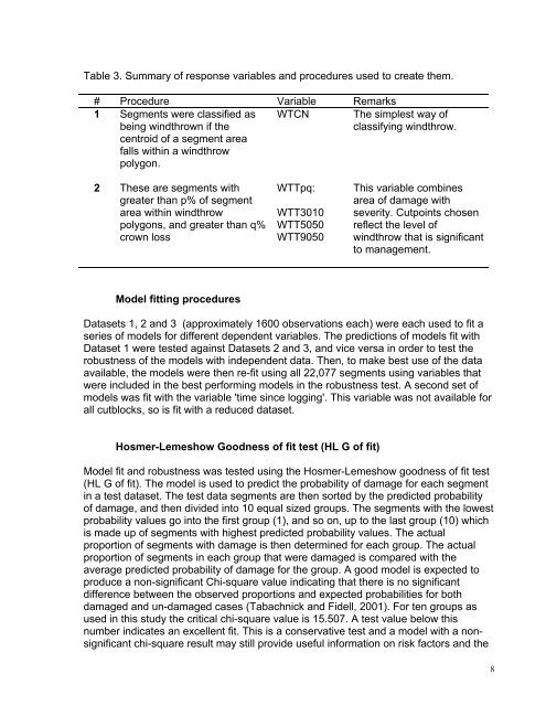
Table 3. Summary of response variables and procedures used to create them.# Procedure Variable Remarks1 Segments were classified asbeing windthrown if thecentroid of a segment areafalls within a windthrowpolygon.WTCN The simplest way ofclassifying windthrow.2 These are segments withgreater than p% of segmentarea within windthrowpolygons, and greater than q%crown lossWTTpq:WTT3010WTT5050WTT9050This variable combinesarea of damage withseverity. Cutpoints chosenreflect the level ofwindthrow that is significantto management.Model fitting proceduresDatasets 1, 2 and 3 (approximately 1600 observations each) were each used to fit aseries of models for different dependent variables. The predictions of models fit withDataset 1 were tested against Datasets 2 and 3, and vice versa in order to test therobustness of the models with independent data. Then, to make best use of the dataavailable, the models were then re-fit using all 22,077 segments using variables thatwere included in the best performing models in the robustness test. A second set ofmodels was fit with the variable 'time since logging'. This variable was not available forall cutblocks, so is fit with a reduced dataset.Hosmer-Lemeshow Goodness of fit test (HL G of fit)Model fit and robustness was tested using the Hosmer-Lemeshow goodness of fit test(HL G of fit). The model is used to predict the probability of damage for each segmentin a test dataset. The test data segments are then sorted by the predicted probabilityof damage, and then divided into 10 equal sized groups. The segments with the lowestprobability values go into the first group (1), and so on, up to the last group (10) whichis made up of segments with highest predicted probability values. The actualproportion of segments with damage is then determined for each group. The actualproportion of segments in each group that were damaged is compared with theaverage predicted probability of damage for the group. A good model is expected toproduce a non-significant Chi-square value indicating that there is no significantdifference between the observed proportions and expected probabilities for bothdamaged and un-damaged cases (Tabachnick and Fidell, 2001). For ten groups asused in this study the critical chi-square value is 15.507. A test value below thisnumber indicates an excellent fit. This is a conservative test and a model with a nonsignificantchi-square result may still provide useful information on risk factors and the8