A Dynamic Model of Housing Supply

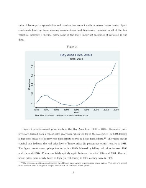
ates of house price appreciation and construction are not uniform across census tracts. Spaceconstraints limit me from showing cross-sectional and time-series variation in all of the keyvariables, however, I include below some of the more important measures of variation in thedata.Figure 2:Bay Area Price levels1988−2004Price level1 1.2 1.4 1.6 1.81988 1990 1992 1994 1996 1998 2000 2002 2004YearNote: Real price levels. 1988 real price level normalized to oneFigure 2 reports overall price levels in the Bay Area from 1988 to 2004. Estimated pricelevels are derived from a repeat sales analysis in which the log of the sales price (in 2000 dollars)is regressed on a set of county-year fixed effects as well as house fixed effects. 20 The values on thevertical axis indicate the real price level of house prices (in percentage terms) relative to 1988.The figure reveals a run up in prices in the late 1980s followed by falling real prices between 1990and the mid-1990s. Prices rose fairly quickly again between the mid-1990s and 2004. Overall,house prices were nearly twice as high (in real terms) in 2004 as they were in 1988.20 The section on estimation discusses the different approaches to measuring house prices. The use of a repeatsales analysis here is to give a simple illustration of trends in house prices.12