A Dynamic Model of Housing Supply

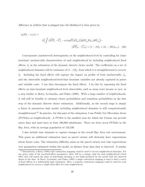
difference in utilities that is plugged into the likelihood is then given by:v 0 (Ω) − v 1 (x) =β( ∫ (ÊP′ n − Ĉ′ n − σ ɛ log[̂P 1 (Ω ′ nj)] )̂q(Ω ′ nj|Ω nj )dΩ ′ nj)−(ÊP nt − Ĉnt) + (1 − β)δ j + (δ t − βE t δ t+1 ) (24)I incorporate (unobserved) heterogeneity at the neighborhood level by controlling for (timeinvariant) unobservable characteristics of each neighborhood by including neighborhood fixedeffects, δ j in the estimation of the dynamic discrete choice model. The coefficients on a set ofneighborhood dummies will be estimates of (1 − β)δ j , from which it is straightforward to recoverδ j . Including the fixed effects will capture the impact on profits of both unobservable, ξ j ,and the observable neighborhood-level-time invariant variables not already captured in pricesand variable costs. I can then decompose the fixed effects. I do this by regressing the fixedeffects on time-invariant neighborhood level observables, such as mean tract income or race, ina step similar to Berry, Levinsohn, and Pakes (1995). With a large number of neighborhoods,it will still be feasible to estimate choice probabilities and transition probabilities in the firststep of the dynamic discrete choice estimation.Additionally, as the second stage is simplya linear in parameters logit model, including neighborhood dummies is still computationallystraightforward. 45 In practice, for this part of the estimation, I use Public Use Microdata Areas(PUMAs) as neighborhoods. A PUMA is the smallest area for which the Census can providemicro data and must have at least 100,000 inhabitants. There are forty seven PUMAs in theBay Area, with an average population of 123,539.I also include time dummies to capture changes in the overall Bay Area cost environment.This poses an additional estimation issue as parcel owners will obviously have expectationsabout future costs. The estimation difficulty arises as the parcel owners now take expectationsover parameters estimated within the model, as distinct from data that is observed. A similar45 Alternatively, a Berry (1994) style contraction mapping could be used to recover neighborhood dummies. Forany given value of the non-fixed-effect parameters, there will be a unique value for each neighborhood’s fixedeffect that will match the share of individuals choosing to not build predicted by the model with the observedshares in the data. In Berry, Levinsohn, and Pakes (1995) a single contraction mapping is used to find a vectorof fixed effects in a multinomial logit estimation. Here, a separate contraction mapping could be used for eachneighborhood to recover a single fixed effect for each neighborhood.30