A Dynamic Model of Housing Supply

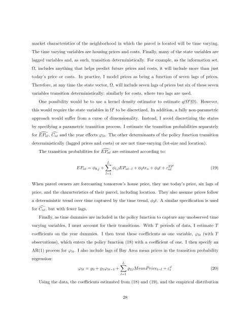
market characteristics of the neighborhood in which the parcel is located will be time varying.The time varying variables are housing prices and costs. Finally, many of the state variables arelagged variables and, as such, transition deterministically. For example, as the information set,Ω, includes anything that helps predict future prices and costs, it will include more than justtoday’s price or costs. In practice, I model prices as being a function of seven lags of prices.Therefore, at any time the state vector, Ω, will include seven lags of prices but six of these sevenvariables transition deterministically: similarly for costs, where two lags are used.One possibility would be to use a kernel density estimator to estimate q(Ω ′ |Ω). However,this would require the state variables in Ω ′ to be discretized. In addition, a fully non-parametricapproach would suffer from a curse of dimensionality. Instead, I avoid discretizing the statesby specifying a parametric transition process. I estimate the transition probabilities separatelyfor ÊP nt , Ĉnt and the year effects ϕ 5t . The other determinants of the policy function transitiondeterministically (lagged prices and costs) or are not time-varying (lot-size and location).The transition probabilities for ÊP nt are estimated according to:EP nt = φ 0,j +L∑l=1φ 1,l EP nt−l + φ 2 ′x n + φ 3 t + ε EPnt (19)When parcel owners are forecasting tomorrow’s house price, they use today’s price, six lags ofprice, and the characteristics of their parcel, including location. They also assume prices followa deterministic trend over time captured by the time trend, φ 3 t. A similar specification is usedfor Ĉnt, but with fewer lags.Finally, as time dummies are included in the policy function to capture any unobserved timevarying variables, I must account for their transitions. With T periods of data, I estimate Tcoefficients on the year dummies. I then treat these coefficients as one variable, ϕ 5t (with Tobservations), which enters the policy function (18) with a coefficient of one. I then specify anAR(1) process for ϕ 5t . I also include lags of Bay Area mean prices in the transition probabilityregression:L∑ϕ 5t = ϱ 0 + ϱ 1 ϕ 5t−1 + ϱ 2,l MeanP rice t−l + ε ϕ t (20)l=1Using the data, the coefficients estimated from (18) and (19), and the empirical distribution28