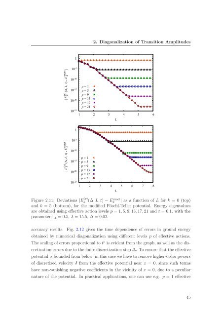
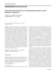
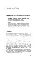
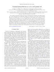
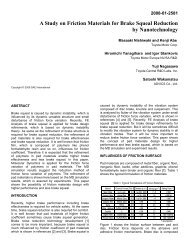
||2. Diagonalization of Transition Amplitudes| E 0(p) (∆, L, t) - E 0exact10 -5 110 -1010 -1510 -2010 -25p = 1p = 5p = 9p = 13p = 17p = 211 2 3 4 5 6L| E 5(p) (∆, L, t) - E 5exact10 -5 110 -1010 -1510 -2010 -25p = 1p = 5p = 9p = 13p = 17p = 211 2 3 4 5 6 7 8LFigure 2.11: Deviations |E (p)k(∆, L, t) − Eexact k | as a function of L for k = 0 (top)and k = 5 (bottom), for the modified Pöschl-Teller potential. Energy eigenvaluesare obta<strong>in</strong>ed us<strong>in</strong>g effective action levels p = 1, 5, 9, 13, 17, 21 and t = 0.1, with theparameters χ = 0.5, λ = 15.5, ∆ = 0.02.accuracy results. Fig. 2.12 gives the time dependence of errors <strong>in</strong> ground energyobta<strong>in</strong>ed by numerical diagonalization us<strong>in</strong>g different levels p of effective actions.The scal<strong>in</strong>g of errors proportional to t p is evident from the graph, as well as the discretizationerrors due to the f<strong>in</strong>ite discretization step ∆. To ensure that the effectivepotential is bounded from below, <strong>in</strong> this case we have to remove higher-order powersof discretized velocity δ from the effective potential near x = 0, s<strong>in</strong>ce such termshave non-vanish<strong>in</strong>g negative coefficients <strong>in</strong> the vic<strong>in</strong>ity of x = 0, due to a peculiarnature of the potential. In practical applications, one can use e.g. p = 1 effective45
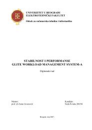
|2. Diagonalization of Transition Amplitudes10 5 0.001 0.01 0.1| E 0(p) (∆, L, t) - E 0exact10 -5 110 -1010 -1510 -20∆ = 0.05∆ = 0.10∆ = 0.2010 -25Figure 2.12: Deviations |E (p)k(∆, L, t) − Eexact k | as a function of t for k = 0, for themodified Pöschl-Teller potential. Energy eigenvalues are obta<strong>in</strong>ed us<strong>in</strong>g effectiveaction levels p = 1, 3, 5, 7, 9, 11, 13 and L = 5, with the parameters χ = 0.5, λ = 15.5,∆ = 0.02. Dashed l<strong>in</strong>es <strong>in</strong> correspond to the discretization error (2.19).taction (which does not depend on δ) near x = 0. As can be seen, this does not affectthe obta<strong>in</strong>ed numerical results.Table 2.3(top) gives the obta<strong>in</strong>ed energy spectra for the modified Pöschl-Tellerpotential with the parameters χ = 0.5, λ = 15.5. If necessary, the precision ofobta<strong>in</strong>ed energy levels can be further <strong>in</strong>creased by appropriately chang<strong>in</strong>g the discretizationparameters. Contrary to the situation for anharmonic oscillator, whererelative error of numerically calculated low-ly<strong>in</strong>g energy levels did not change significantly,here we see that the <strong>in</strong>crease <strong>in</strong> the error is substantial. This is causedby the fact that this potential has only a small f<strong>in</strong>ite set of discrete bound states, soenergy levels k ∼ 10 correspond to the very top of the discrete spectrum. In practicalapplications such pathological situations are not encountered, but as we can see,even this can be dealt with by the proper choice of discretization parameters. Thequality of numerically calculated eigenfunctions is assessed <strong>in</strong> Table 2.3(bottom),where we give a symmetric matrix of scalar products 〈ψ k |ψlexact 〉 of numerically calculatedand analytic eigenfunctions. As we can see, the overlap between analyticand numeric eigenfunctions is excellent, and they are orthogonal with high precision,which is preserved even for higher energy levels. We have also verified that forparameters given <strong>in</strong> the caption of Table 2.3 and with the discretization step of theorder ∆ = 10 −3 eigenfunctions of all bound states can be accurately reproduced.46
- Page 1 and 2:
UNIVERSITY OF BELGRADEFACULTY OF PH
- Page 3 and 4:
Thesis advisor, Committee member:Dr
- Page 6 and 7:
lence for Computer Modeling of Comp
- Page 8 and 9:
dobijanje kondenzata odabrani su at
- Page 10 and 11:
Uticaj slabih interakcija na fenome
- Page 12 and 13:
Abstract of the doctoral dissertati
- Page 14 and 15:
highly accurate information on ener
- Page 16 and 17: Keywords: cold quantum gases, Bose-
- Page 18 and 19: CONTENTS3.4.2 Time-of-flight graphs
- Page 20 and 21: NomenclatureRoman Symbolsagk BLMNn(
- Page 22 and 23: Chapter 1Introduction1.1 ForewordTh
- Page 24 and 25: ently explored to illustrate the ve
- Page 26 and 27: Summations in the last expression c
- Page 28 and 29: Figure 1.1: The hallmark of the Bos
- Page 30 and 31: we discuss in some detail the exper
- Page 32 and 33: In the first papers [3, 4], the TOF
- Page 34 and 35: where a BG is the off-resonant scat
- Page 36 and 37: system given by( ) ǫ Bog ⃗k =
- Page 38 and 39: Having the efficient numerical meth
- Page 40 and 41: Chapter 2Properties of quantum syst
- Page 42 and 43: 2. Diagonalization of Transition Am
- Page 44 and 45: 2. Diagonalization of Transition Am
- Page 46 and 47: 2. Diagonalization of Transition Am
- Page 48 and 49: 2. Diagonalization of Transition Am
- Page 50 and 51: 2. Diagonalization of Transition Am
- Page 52 and 53: 2. Diagonalization of Transition Am
- Page 54 and 55: 2. Diagonalization of Transition Am
- Page 56 and 57: 2. Diagonalization of Transition Am
- Page 58 and 59: 2. Diagonalization of Transition Am
- Page 60 and 61: 2. Diagonalization of Transition Am
- Page 62 and 63: 2. Diagonalization of Transition Am
- Page 64 and 65: 2. Diagonalization of Transition Am
- Page 68 and 69: 2. Diagonalization of Transition Am
- Page 70 and 71: 2. Diagonalization of Transition Am
- Page 72 and 73: 2. Diagonalization of Transition Am
- Page 74: 2. Diagonalization of Transition Am
- Page 77 and 78: 2. Diagonalization of Transition Am
- Page 79 and 80: magnetic field ⃗ B = 2M ⃗ Ω.3.
- Page 81 and 82: 3. Rotating ideal BECof the rotatio
- Page 83 and 84: 3. Rotating ideal BEC3.1 Numerical
- Page 85 and 86: 3. Rotating ideal BEC350300SC appro
- Page 87 and 88: 3. Rotating ideal BEC3.2 Finite num
- Page 89 and 90: 3. Rotating ideal BECN - N 03.0·10
- Page 91 and 92: 3. Rotating ideal BEC3.3 Global pro
- Page 93 and 94: 3. Rotating ideal BECever, it does
- Page 95 and 96: 3. Rotating ideal BECT c [nK]120110
- Page 97 and 98: 3. Rotating ideal BEC3.533210 3 κ
- Page 99 and 100: 3. Rotating ideal BECn(x, y)10·10
- Page 101 and 102: 3. Rotating ideal BECpancy numbers
- Page 103 and 104: 3. Rotating ideal BEC6·10 4 0 0.02
- Page 105 and 106: Chapter 4Mean-field description of
- Page 107 and 108: 4. Mean-field description of an int
- Page 109 and 110: 4. Mean-field description of an int
- Page 111 and 112: 4. Mean-field description of an int
- Page 113 and 114: 4. Mean-field description of an int
- Page 115 and 116: 4. Mean-field description of an int
- Page 117 and 118:
4. Mean-field description of an int
- Page 119 and 120:
4. Mean-field description of an int
- Page 121 and 122:
4. Mean-field description of an int
- Page 123 and 124:
4. Mean-field description of an int
- Page 125 and 126:
Chapter 5Nonlinear BEC dynamics by
- Page 127 and 128:
5. BEC excitation by modulation of
- Page 129 and 130:
5. BEC excitation by modulation of
- Page 131 and 132:
5. BEC excitation by modulation of
- Page 133 and 134:
5. BEC excitation by modulation of
- Page 135 and 136:
5. BEC excitation by modulation of
- Page 137 and 138:
5. BEC excitation by modulation of
- Page 139 and 140:
5. BEC excitation by modulation of
- Page 141 and 142:
5. BEC excitation by modulation of
- Page 143 and 144:
5. BEC excitation by modulation of
- Page 145 and 146:
5. BEC excitation by modulation of
- Page 147 and 148:
5. BEC excitation by modulation of
- Page 149 and 150:
where n = 1, 2, 3, . . . is an inte
- Page 151 and 152:
5. BEC excitation by modulation of
- Page 153 and 154:
5. BEC excitation by modulation of
- Page 155 and 156:
Chapter 6SummarySince the first exp
- Page 157 and 158:
short-range interactions.The excita
- Page 159 and 160:
of the ground state. Imaginary-time
- Page 161 and 162:
(A.13). With another boundary condi
- Page 163 and 164:
Appendix B Time-dependent variation
- Page 165 and 166:
List of papers by Ivana VidanovićT
- Page 167 and 168:
References[1] S. N. Bose, Plancks g
- Page 169 and 170:
REFERENCES[21] W. Ketterle, D. S. D
- Page 171 and 172:
REFERENCES[45] A. Bogojević, A. Ba
- Page 173 and 174:
REFERENCES[70] M. R. Matthews, B. P
- Page 175 and 176:
REFERENCES[94] M.-O. Mewes, M. R. A
- Page 177 and 178:
REFERENCES[116] K. Staliunas, S. Lo
- Page 179 and 180:
CURRICULUM VITAE - Ivana Vidanović