
Create successful ePaper yourself
Turn your PDF publications into a flip-book with our unique Google optimized e-Paper software.
MAGYAR NEMZETI BANK<br />
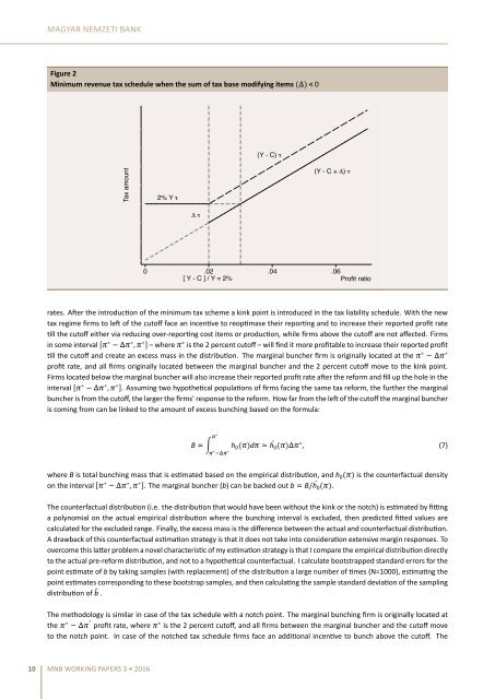
Figure 2<br />
Minimum revenue tax schedule when the sum of tax base modifying items () < 0<br />
Tax amount<br />
0 .01 .02 .03 .04 .05 .06 .07<br />
2% Y τ<br />
Δ τ<br />
(Y - C) τ<br />
(Y - C + Δ) τ<br />
0 .02 .04 .06<br />
[ Y - C ] / Y = 2%<br />
Profit ratio<br />
rates. Aer the introducon of the minimum tax scheme a kink point is introduced in the tax liability schedule. With the new<br />
tax regime firms to le of the cutoff face an incenve to reopmase their reporng and to increase their reported profit rate<br />
ll the cutoff either via reducing over-reporng cost items or producon, while firms above the cutoff are not affected. Firms<br />
in some interval [ ∗ ∗ , ∗ ] – where ∗ is the 2 percent cutoff – will find it more profitable to increase their reported profit<br />
ll the cutoff and create an excess mass in the distribuon. The marginal buncher firm is originally located at the ∗ ∗<br />
profit rate, and all firms originally located between the marginal buncher and the 2 percent cutoff move to the kink point.<br />
Firms located below the marginal buncher will also increase their reported profit rate aer the reform and fill up the hole in the<br />
interval [ ∗ ∗ , ∗ ]. Assuming two hypothecal populaons of firms facing the same tax reform, the further the marginal<br />
buncher is <strong>from</strong> the cutoff, the larger the firms’ response to the reform. How far <strong>from</strong> the le of the cutoff the marginal buncher<br />
is coming <strong>from</strong> can be linked to the amount of excess <strong>bunching</strong> based on the formula:<br />
∗<br />
B h 0 ()d ≃ h 0<br />
̄ () ∗ , (7)<br />
∗ ∗<br />
where B is total <strong>bunching</strong> mass that is esmated based on the empirical distribuon, and h 0 () is the counterfactual density<br />
on the interval [ ∗ ∗ , ∗ ]. The marginal buncher (b) can be backed out b B/ h 0<br />
̄ ().<br />
The counterfactual distribuon (i.e. the distribuon that would have been without the kink or the notch) is esmated by fing<br />
a polynomial on the actual empirical distribuon where the <strong>bunching</strong> interval is excluded, then predicted fied values are<br />
calculated for the excluded range. Finally, the excess mass is the difference between the actual and counterfactual distribuon.<br />
A drawback of this counterfactual esmaon strategy is that it does not take into consideraon extensive margin responses. To<br />
overcome this laer problem a novel characterisc of my esmaon strategy is that I compare the empirical distribuon directly<br />
to the actual pre-reform distribuon, and not to a hypothecal counterfactual. I calculate bootstrapped standard errors for the<br />
point esmate of b by taking samples (with replacement) of the distribuon a large number of mes (N=1000), esmang the<br />
point esmates corresponding to these bootstrap samples, and then calculang the sample standard deviaon of the sampling<br />
distribuon of b .<br />
The methodology is similar in case of the tax schedule with a notch point. The marginal <strong>bunching</strong> firm is originally located at<br />
the ∗ <br />
profit rate, where ∗ is the 2 percent cutoff, and all firms between the marginal buncher and the cutoff move<br />
to the notch point. In case of the notched tax schedule firms face an addional incenve to bunch above the cutoff. The<br />
10 MNB WORKING PAPERS 3 • 2016