Computer Algebra Recipes

2.1. PHASE-PLANE ANALYSIS 53
> a:=a; b:=b; c:=c; d:=d;
a := 0 b := ¡3 c := 2
d := 0
3
The quantities p = ¡(a + d) andq = ad¡ bc are calculated.
> p:=-(a+d); q:=a*d-b*c;
p := 0 q := 2
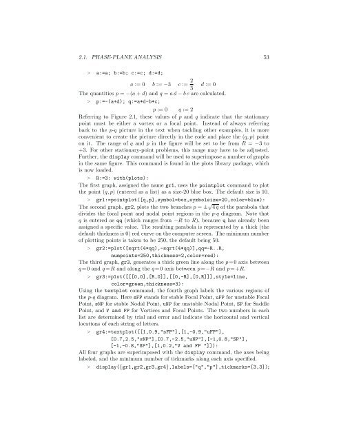
Referring to Figure 2.1, these values of p and q indicate that the stationary
point must be either a vortex or a focal point. Instead of always referring
back to the p-q picture in the text when tackling other examples, it is more
convenient to create the picture directly in the code and place the (q, p) point
on it. The range of q and p in the ¯gure will be set to be from R = ¡3 to
+3. For other stationary-point problems, this range may have to be adjusted.
Further, the display command will be used to superimpose a number of graphs
in the same ¯gure. This command is found in the plots library package, which
is now loaded.
> R:=3: with(plots):
The ¯rst graph, assigned the name gr1, usesthepointplot command to plot
the point (q, p) (entered as a list) as a size-20 blue box. The default size is 10.
> gr1:=pointplot([q,p],symbol=box,symbolsize=20,color=blue):
The second graph, gr2, plotsthetwobranchesp = § p 4 q of the parabola that
divides the focal point and nodal point regions in the p-q diagram. Note that
q is entered as qq (which ranges from ¡R to R), because q has already been
assigned a speci¯c value. The resulting parabola is represented by a thick (the
default thickness is 0) red curve on the computer screen. The minimum number
of plotting points is taken to be 250, the default being 50.
> gr2:=plot([sqrt(4*qq),-sqrt(4*qq)],qq=-R..R,
numpoints=250,thickness=2,color=red):
The third graph, gr3, generates a thick green line along the p=0 axis between
q =0 andq =R and along the q =0 axis between p=¡R and p=+R.
> gr3:=plot([[[0,0],[R,0]],[[0,-R],[0,R]]],style=line,
color=green,thickness=3):
Using the textplot command, the fourth graph labels the various regions of
the p-q diagram. Here sFP stands for stable Focal Point, uFP for unstable Focal
Point, sNP for stable Nodal Point, uNP for unstable Nodal Point, SP for Saddle
Point, and V and FP for Vortices and Focal Points. The two numbers in each
list are determined by trial and error and indicate the horizontal and vertical
locations of each string of letters.
> gr4:=textplot([[1,0.9,"sFP"],[1,-0.9,"uFP"],
[0.7,2.5,"sNP"],[0.7,-2.5,"uNP"],[-1,0.8,"SP"],
[-1,-0.8,"SP"],[1,0.2,"V and FP "]]):
All four graphs are superimposed with the display command, the axes being
labeled, and the minimum number of tickmarks along each axis speci¯ed.
> display(fgr1,gr2,gr3,gr4g,labels=["q","p"],tickmarks=[3,3]);