SOLWEIG 1.0 – Modelling spatial variations of 3D radiant fluxes and ...
SOLWEIG 1.0 – Modelling spatial variations of 3D radiant fluxes and ...
SOLWEIG 1.0 – Modelling spatial variations of 3D radiant fluxes and ...

Create successful ePaper yourself
Turn your PDF publications into a flip-book with our unique Google optimized e-Paper software.
710 Int J Biometeorol (2008) 52:697<strong>–</strong>713<br />
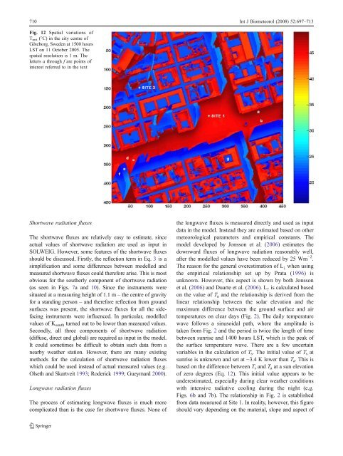
Fig. 12 Spatial <strong>variations</strong> <strong>of</strong><br />
T mrt (°C) in the city centre <strong>of</strong><br />
Göteborg, Sweden at 1500 hours<br />
LST on 11 October 2005. The<br />
<strong>spatial</strong> resolution is 1 m. The<br />
letters a through f are points <strong>of</strong><br />
interest referred to in the text<br />
Shortwave radiation <strong>fluxes</strong><br />
The shortwave <strong>fluxes</strong> are relatively easy to estimate, since<br />
actual values <strong>of</strong> shortwave radiation are used as input in<br />
<strong>SOLWEIG</strong>. However, some features <strong>of</strong> the shortwave <strong>fluxes</strong><br />
should be discussed. Firstly, the reflection term in Eq. 3 is a<br />
simplification <strong>and</strong> some differences between modelled <strong>and</strong><br />
measured shortwave <strong>fluxes</strong> could therefore arise. This is most<br />
obvious for the southerly component <strong>of</strong> shortwave radiation<br />
(asseeninFigs.7a <strong>and</strong>10). Since the instruments were<br />
situated at a measuring height <strong>of</strong> 1.1 m <strong>–</strong> the centre <strong>of</strong> gravity<br />
for a st<strong>and</strong>ing person <strong>–</strong> <strong>and</strong> therefore reflection from ground<br />
surfaces was present, the shortwave <strong>fluxes</strong> for all the sidefacing<br />
instruments were influenced. In particular, modelled<br />
values <strong>of</strong> K south turned out to be lower than measured values.<br />
Secondly, all three components <strong>of</strong> shortwave radiation<br />
(diffuse, direct <strong>and</strong> global) are required as input in the model.<br />
It could sometimes be difficult to obtain such data from a<br />
nearby weather station. However, there are many existing<br />
methods for the calculation <strong>of</strong> shortwave radiation <strong>fluxes</strong><br />
which could be used instead <strong>of</strong> actual measured values (e.g.<br />
Olseth <strong>and</strong> Skartveit 1993; Roderick 1999; Gueymard 2000).<br />
Longwave radiation <strong>fluxes</strong><br />
The process <strong>of</strong> estimating longwave <strong>fluxes</strong> is much more<br />
complicated than is the case for shortwave <strong>fluxes</strong>. None <strong>of</strong><br />
the longwave <strong>fluxes</strong> is measured directly <strong>and</strong> used as input<br />
data in the model. Instead they are estimated based on other<br />
meteorological parameters <strong>and</strong> empirical constants. The<br />
model developed by Jonsson et al. (2006) estimates the<br />
downward <strong>fluxes</strong> <strong>of</strong> longwave radiation reasonably well,<br />
after the modelled values have been reduced by 25 Wm −2 .<br />
The reason for the general overestimation <strong>of</strong> L↓ when using<br />
the empirical relationship set up by Prata (1996) is<br />
unknown. However, this aspect is shown by both Jonsson<br />
et al. (2006) <strong>and</strong> Duarte et al. (2006). L↑ is calculated based<br />
on the value <strong>of</strong> Ta <strong>and</strong> the relationship is derived from the<br />
linear relationship between the solar elevation <strong>and</strong> the<br />
maximum difference between the ground surface <strong>and</strong> air<br />
temperatures on clear days (Fig. 2). The daily temperature<br />
wave follows a sinusoidal path, where the amplitude is<br />
taken from Fig. 2 <strong>and</strong> the period is twice the length <strong>of</strong> time<br />
between sunrise <strong>and</strong> 1400 hours LST, which is the peak <strong>of</strong><br />
the surface temperature wave. There are a few uncertain<br />
variables in the calculation <strong>of</strong> Ts. The initial value <strong>of</strong> Ts at<br />
sunrise is unknown <strong>and</strong> set at −3.4 K lower than Ta. This is<br />
based on the difference between T s <strong>and</strong> T a at a sun elevation<br />
<strong>of</strong> zero degrees (Eq. 12). This initial value appears to be<br />
underestimated, especially during clear weather conditions<br />
with intensive radiative cooling during the night (e.g.<br />
Figs. 6b <strong>and</strong> 7b). The relationship in Fig. 2 is established<br />
from data measured at Site 1. In reality, however, this figure<br />
should vary depending on the material, slope <strong>and</strong> aspect <strong>of</strong>