Three-dimensional Lagrangian Tracer Modelling in Wadden Sea ...

CHAPTER 2. THEORY 9
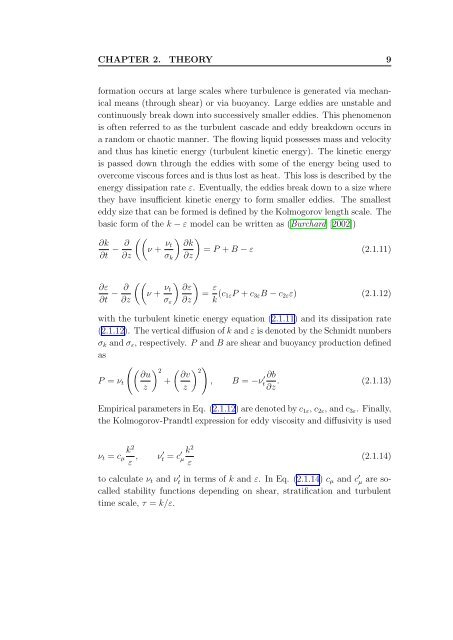
formation occurs at large scales where turbulence is generated via mechanical
means (through shear) or via buoyancy. Large eddies are unstable and
continuously break down into successively smaller eddies. This phenomenon
is often referred to as the turbulent cascade and eddy breakdown occurs in
a random or chaotic manner. The flowing liquid possesses mass and velocity
and thus has kinetic energy (turbulent kinetic energy). The kinetic energy
is passed down through the eddies with some of the energy being used to
overcome viscous forces and is thus lost as heat. This loss is described by the
energy dissipation rate ε. Eventually, the eddies break down to a size where
they have insufficient kinetic energy to form smaller eddies. The smallest
eddy size that can be formed is defined by the Kolmogorov length scale. The
basic form of the k − ε model can be written as (Burchard [2002])
∂k
∂t
− ∂
∂z
��
ν + νt
σk
� ∂k
∂z
�
= P + B − ε (2.1.11)
��
∂ε ∂
− ν +
∂t ∂z
νt
� �
∂ε
=
σε ∂z
ε
k (c1εP + c3εB − c2εε) (2.1.12)
with the turbulent kinetic energy equation (2.1.11) and its dissipation rate
(2.1.12). The vertical diffusion of k and ε is denoted by the Schmidt numbers
σk and σε, respectively. P and B are shear and buoyancy production defined
as
��∂u �2 � � �
2
∂v
P = νt + , B = −ν
z z
′ ∂b
t . (2.1.13)
∂z
Empirical parameters in Eq. (2.1.12) are denoted by c1ε, c2ε, and c3ε. Finally,
the Kolmogorov-Prandtl expression for eddy viscosity and diffusivity is used
k
νt = cµ
2
ε , ν′ t = c ′ k
µ
2
ε
(2.1.14)
to calculate νt and ν ′ t in terms of k and ε. In Eq. (2.1.14) cµ and c ′ µ are socalled
stability functions depending on shear, stratification and turbulent
time scale, τ = k/ε.