Three-dimensional Lagrangian Tracer Modelling in Wadden Sea ...

CHAPTER 2. THEORY 13
j
∆y
k
i
i
∆x
H, ζ, k, ε, ν , ν'
u, U
v, V
ρ, C i
u
w, k, ε, ν , ν'
t t
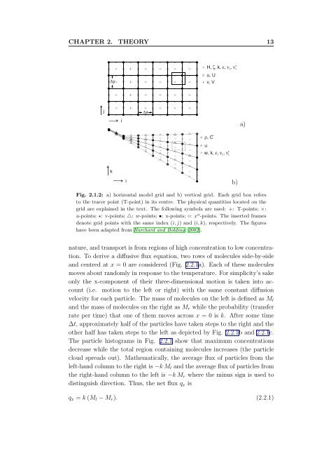
Fig. 2.1.2: a) horizontal model grid and b) vertical grid. Each grid box refers
to the tracer point (T-point) in its centre. The physical quantities located on the
grid are explained in the text. The following symbols are used: +: T-points; ×:
u-points; ⋆: v-points; △: w-points; •: x-points; ◦: x u -points. The inserted frames
denote grid points with the same index (i, j) and (i, k), respectively. The figures
have been adapted from Burchard and Bolding [2002].
nature, and transport is from regions of high concentration to low concentration.
To derive a diffusive flux equation, two rows of molecules side-by-side
and centred at x = 0 are considered (Fig. 2.2.1a). Each of these molecules
moves about randomly in response to the temperature. For simplicity’s sake
only the x-component of their three-dimensional motion is taken into account
(i.e. motion to the left or right) with the same constant diffusion
velocity for each particle. The mass of molecules on the left is defined as Ml
and the mass of molecules on the right as Mr while the probability (transfer
rate per time) that one of them moves across x = 0 is k. After some time
∆t, approximately half of the particles have taken steps to the right and the
other half has taken steps to the left as depicted by Fig. 2.2.1b and 2.2.1c.
The particle histograms in Fig. 2.2.1 show that maximum concentrations
decrease while the total region containing molecules increases (the particle
cloud spreads out). Mathematically, the average flux of particles from the
left-hand column to the right is −k Ml and the average flux of particles from
the right-hand column to the left is −k Mr where the minus sign is used to
distinguish direction. Thus, the net flux qx is
qx = k (Ml − Mr). (2.2.1)
t
t
b)
a)