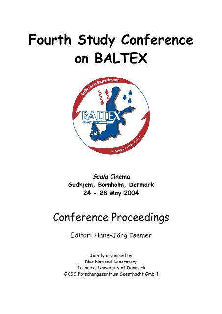
Fourth Study Conference on BALTEX Scala Cinema Gudhjem

<strong>Fourth</strong> <strong>Study</strong> <strong>Conference</strong>
on BALTEX
Scala Cinema
Gudhjem, Bornholm, Denmark
24 - 28 May 2004
<strong>Conference</strong> Proceedings
Editor: Hans-Jörg Isemer
Jointly organised by
Risø National Laboratory
Technical University of Denmark
GKSS Forschungszentrum Geesthacht GmbH

<strong>Conference</strong> Committee
Hartmut Graßl, MPI for Meteorology, Germany
Sven-Erik Gryning, Risø National Laboratory, Denmark
Hans-Jörg Isemer, GKSS Research Centre, Germany
Sirje Keevallik, Estonian Maritime Academy, Estonia
Andreas Lehmann, IfM Kiel, Germany
Anders Lindroth, Lund University, Sweden
Anders Omstedt, Göteborg University, Sweden
Dan Rosbjerg, Technical University of Denmark
Markku Rummukainen, SMHI, Sweden
Clemens Simmer, Bonn University, Germany

Preface
The 4 th <strong>Study</strong> <strong>Conference</strong> on BALTEX takes place at an important point of time of the programme.
After about 10 years of successful research dedicated to a better understanding of the
water and energy cycles of the Baltic Sea basin, BALTEX has recently defined revised objectives
for Phase II of the programme. A future focus of BALTEX will be on applications of its
past achievements to other fields, both in science research and beyond, where knowledge of
the water and energy cycle is of fundamental importance. Some of this <strong>Conference</strong>’s sessions
already reflect aspects of the revised BALTEX objectives for Phase II, such as investigations
on past and future climate as well as contributions to water resource management. At the <strong>Conference</strong>,
more than 110 presentations will be given originating from institutions and groups in
15 countries.
Timing and location of this <strong>Conference</strong> follow a meanwhile established BALTEX tradition:
The conduction of BALTEX <strong>Conference</strong>s on Baltic Sea islands in three years intervals. Following
previous BALTEX <strong>Study</strong> <strong>Conference</strong>s on Gotland in 1995, Rügen in 1998 and Åland
in 2001, the BALTEX community is assembling on the Danish island of Bornholm now in
2004. The <strong>Conference</strong> venue is the Scala Cinema in Gudhjem, a beautiful little fishing village
at the north-east coast of Bornholm.
This proceeding volume contains abstracts of all papers, both oral presentations and posters,
given at the <strong>Conference</strong>. They are ordered according to the <strong>Conference</strong> sessions and the <strong>Conference</strong>
programme (see separate booklet).
The conference has jointly been organized by the International BALTEX Secretariat at GKSS
Forschungszentrum Geesthacht GmbH, Risø National Laboratory and the Technical University
of Denmark. Local preparations for the <strong>Conference</strong> have significantly been supported by
Bornholms Booking Centre in Allinge. I like to thank particularly Hanne Vang, Hans Jørgen
Jensen, Henrik Hansen and Silke Köppen for their enthusiastic engagement.
Geesthacht, May 2004
Hans-Jörg Isemer
Editor

Sponsors of the <strong>Conference</strong> include:
Risø National Laboratory
Technical University of Denmark
GKSS Forschungszentrum Geesthacht GmbH
Gesellschaft zur Förderung des GKSS Forschungszentrums e.V.
Max-Planck-Institut für Meteorologie Hamburg
European Association for the Science of Air Pollution
(EURASAP)
Their support of the <strong>Conference</strong> is gratefully acknowledged.

- I -
Table of Abstracts
Title
Authors.......................................................................................................................................page
Activities of the GEWEX Hydrometeorology Panel GHP
John Roads ....................................................................................................................................................1
The Coordinated Enhanced Observing Period CEOP
Hartmut Graßl ...............................................................................................................................................2
BONUS for the Baltic Sea Science - Network of Funding Agencies
Kaisa Kononen ..............................................................................................................................................4
Remote Sensing of Atmospheric Properties above the Baltic Region
Jürgen Fischer, P. Albert, R. Preusker (Invited)............................................................................................5
Review of Major CLIWA-NET Results
Erik van Meijgaard, S. Crewell, A. Feijt, C. Simmer (Invited).....................................................................6
North European Radar Products and Research for BALTEX
Jarmo Koistinen, D. B. Michelson ................................................................................................................8
Precipitation Type Statistics in the Baltic Region Derived from Three Years of BALTEX Radar
Data Centre (BRDC) Data
Ralf Bennartz, A. Walther.............................................................................................................................9
Cloud Properties Above the Baltic Region
Rene Preusker, L. Schüller, J. Fischer.........................................................................................................10
Assimilation of New Land Surface Data Sets in Weather Prediction Models
Matthias Drusch (Invited)............................................................................................................................11
A Continental Scale Soil Moisture Retrieval Algorithm, ist Derivation and its Application to
Model Data
Ralf Lindau, C. Simmer ..............................................................................................................................12
Analysis of Model Predicted Liquid Water Path and Liquid Water Vertical Distribution using
Observations from CLIWA-NET
Erik van Meijgaard, S. Crewell, U. Löhnert................................................................................................14
Vertical Structure and Weather Radar Estimation of Rain
Gerhard Peters, B. Fischer...........................................................................................................................16
Comparison of Model and Cloud Radar Derived Cloud Vertical Structure and Overlap for the
BALTEX BRIDGE Campaign.
Ulrika Willén...............................................................................................................................................18
CERES and Surface Radiation Budget Data for BALTEX
G. Louis Smith, B. A. Wielicki, P. W. Stackhouse.....................................................................................19

- II -
Coastal Wind Mapping from Satellite SAR: Possibilities and Limitations
Charlotte B. Hasager, M. B. Christiansen ...................................................................................................21
Clouds and Water Vapor over the Baltic Sea 2001-2003: First Results of the new
Preliminary DWD Climate Monitoring Programme
Peter Bissolli, H. Nitsche, W. Rosenow......................................................................................................23
Broadband Cloud Albedo from MODIS
Anja Hünerbein, R. Preusker, J. Fischer .....................................................................................................25
High Frequency Single Board Doppler Minisodar for Rain, Hail, Snow, Graupel and Mixed Phase
Precipitation Measurements
Shixuan Pang, H. Graßl...............................................................................................................................26
Observation of Clouds and Water Vapour with Satellites
Maximilian Reuter, P. Lorenz, J. Fischer....................................................................................................27
GPS-Based Integrated Water Vapour Estimation on Static and Moving
Platforms for Verification of Regional Climate Model REMO
Torben Schüler, A. Posfay, E. Krueger, G. W. Hein, D. Jacob...................................................................28
Validation of Boundary Layer Parameters and Extension of Boundary Conditions of the Climate
Model REMO – Estimation of Leaf Area Index from NOAA-AVHRR-Data
Birgit Streckenbach, E. Reimer...................................................................................................................30
Determination and Comparison of Evapotranspiration with Remote Sensing
and Numerical Modelling in the LITFASS Area
Antje Tittebrand, C. Heret, B. Ketzer, F. H. Berger....................................................................................31
Spatial Variability of Snow Cover and its Implication for the Forest Regeneration at the Northern
Climatological Tree-line (Finnish Lapland)
Andrea Vajda, A. Venäläinen, P. Hänninen, R. Sutinen .............................................................................33
EVA-GRIPS: Regional Evaporation at Grid and Pixel Scale over Heterogeneous Land Surfaces
Heinz-Theo Mengelkamp and the EVA-GRIPS Team (invited).................................................................35
LITFASS-2003 - A Land Surface / Atmosphere Interaction Experiment: Energy and Water Vapour
Fluxes at Different Scales
Frank Beyrich, J. Bange, C. Bernhofer, H. A. R. de Bruin, T. Foken, B. Hennemuth, S. Huneke, W.
Kohsiek, J.-P. Leps, H. Lohse, A. Lüdi, M. Mauder, W. Meijninger, R. Queck, P. Zittel .........................37
Calibrated Surface Temperature Maps of Heterogeneous Terrain Derived from Helipod and
German Air Force Tornado Flights during LITFASS-2003
Jens Bange, S. Wilken, T. Spieß, P. Zittel...................................................................................................39
The Marine Boundary Layer – New Findings from the Östergarnsholm Air-Sea Interaction Site in
the Baltic Sea
Ann-Sofie Smedman, U. Högström (invited)..............................................................................................41
Characteristics of the Atmospheric Boundary Layer over Baltic Sea Ice
Burghard Brümmer, A. Kirchgäßner, G. Müller .........................................................................................43

- III -
Sensitivity in Calculation of Turbulent Fluxes over Sea to the State of the Surface Waves
Anna Rutgersson, A.-S. Smedman, B. Carlsson .........................................................................................44
Is the Critical Bulk Richardson Number Constant ?
Sven-Erik Gryning, E. Batchvarova............................................................................................................46
Measured Drop Size Distributions: Differences over Land and Sea
M. Clemens, K. Bumke...............................................................................................................................48
MESAN Mesoscale Analysis of Total Cloud Cover
Günther Haase, T. Landelius.......................................................................................................................50
A new 3-hourly Precipitation Dataset for NWP Model Verification and Data Assimilation Studies
Franz Rubel, P. Skomorowski, K. Brugger.................................................................................................52
Relationships Between Precipitable Water and Geographical Latitude in the Baltic Region
Erko Jakobson, H. Ohvril, O. Okulov, N. Laulainen ..................................................................................53
Analysis of the Role of Atmospheric Cyclones in the Moisture Transport from the Atlantic Ocean to
Europe and European Precipitation
Irina Rudeva, S. Gulev, O. Zolina, E. Ruprecht..........................................................................................55
Meteorological Peculiarities of Maximum Rainfall-induced Runoff Formation in Lithuania
Egidijus Rimkus, J. Rimkuviene .................................................................................................................57
Baltic Sea Inflow Events
Jan Piechura (invited) ..................................................................................................................................59
The Different Baltic Inflows in Autumn 2002 and Winter 2003
Rainer Feistel, G. Nausch............................................................................................................................61
Observations of Turbulent Kinetic Energy Dissipation in the Surface Mixed Layer of the Baltic Sea
Under Varying Forcing
Hans Ulrich Lass, H. Prandke .....................................................................................................................63
The Impacts of Synoptic Situations on Extreme Precipitation in the Raba Valley
(Gaik-Brzezowa)
Agnieszka Saramak .....................................................................................................................................65
Improved Method for the Determination of Turbulent Surface Fluxes Using Low-Level Flights and
Inverse Modelling
Jens Bange, T. Spieß, P. Zittel ....................................................................................................................67
The Helicopter-Borne Turbulence Probe Helipod in LITFASS Field Campaigns:
Strategies and Results
Peter Zittel, T. Spieß, J. Bange....................................................................................................................69
CEOP Reference Site Data from Lindenberg: Be Aware of Terrain Heterogeneity !
Frank Beyrich, W. K. Adam........................................................................................................................71
The BALTEX Hydrological Data Centre, BHDC
Bengt Carlsson ............................................................................................................................................73

- IV -
Hydrological and Hydrochemical Surface Water Monitoring Network in the Republic of Belarus
Ryhor Chekan, V. Korneev .........................................................................................................................75
Sea-level Monitoring at MARNET Stations in the Southern Baltic Sea
Lutz Eberlein, R. Dietrich, M. Neukamm, G. Liebsch................................................................................77
A Comparison Between the ERA40 and the SMHI Gridded Meteorological Data Bases with
Applications to Baltic Sea Modelling
Anders Omstedt, Y. Chen, K. Wesslander ..................................................................................................78
Evaluation of Atmosphere-ocean Heat Fluxes over the Baltic Sea using a Number of Gridded
Meteorological Databases
Anna Rutgersson, A. Omstedt, G. Nilsson..................................................................................................80
Variability of Ångström Coefficients during Summer in Estonia
Hilda Teral, H. Ohvril, N. Laulainen...........................................................................................................82
BASEWECS – Baltic Sea Water and Energy Cycle
Andreas Lehmann, W. Krauss (invited) ......................................................................................................84
Influence of Atmospheric Forcing on Simulations with a General Circulation Model of the Baltic
Sea
Frank Janssen, T. Seifert .............................................................................................................................85
The BALTEX/BRIDGE Water Budget and Heat Balances Calculated from Baltic Sea Modelling
and Available Meteorological, Hydrological and Ocean Data
Anders Omstedt (invited) ............................................................................................................................86
A 10 Years Simulations of the Baltic Sea Hydrography with Special Attention to the Sea Level
Fluctuations
Kai Myrberg, O. Andrejev, B. Sjöberg .......................................................................................................88
Atypical Coastal Gradients in the Wind Speed and Air Humidity over the Baltic Sea
Timo Vihma ................................................................................................................................................90
On Variability of the Riverine Waters in the Gulf of Gdansk – A Model <strong>Study</strong>
Andrzej Jankowski ......................................................................................................................................92
Operational Hydrodynamic Model for Forecasting of Extreme Hydrological Conditions in the Oder
Estuary
Halina Kowalewska-Kalkowska, M. Kowalewski......................................................................................94
Continental-Scale Water-Balance Modelling of the Baltic and other Large Catchments
Elin Widén, Chong-yu Xu, S. Halldin.........................................................................................................95
ICTS (Inter-CSE Transferability <strong>Study</strong>): An Application of CEOP Data
Burghardt Rockel, J. Roads, I. Meinke .......................................................................................................97
Introducing Lateral Subsurface Flow in Permafrost Conditions in a Distributed Land Surface
Scheme
Petra Koudelova, T. Koike..........................................................................................................................98

- V -
Parameter Estimation of the SVAT Schemes TERRA/LM and REMO/ECHAM using a Multicriteria
Method
Klaus-Peter Johnsen, S. Huneke, J. Geyer, H.-T. Mengelkamp................................................................100
Comparison of Methods for Area-averaging Surface Energy Fluxes over Heterogeneous Land
Surfaces Using High-resolution Nonhydrostatic Simulations
Günther Heinemann, M. Kerschgens ........................................................................................................102
Modelling the Impact of Inertia-Gravity Waves on Wind and Precipitation
Christoph Zülicke, D. Peters .....................................................................................................................103
Objective Calibration of the Land Surface Model SEWAB
Sven Huneke, K.-P. Johnsen, J. Geyer, H. Lohse, H.-T. Mengelkamp.....................................................105
Validation of Boundary Layer Parameters and Extension of Boundary Conditions of Climate Model
REMO – Snow Cover
Michael Woldt, E. Reimer.........................................................................................................................107
Upwelling in the Baltic Sea - A Numerical Model Case <strong>Study</strong> -
Andreas Lehmann, H.-H. Hinrichsen........................................................................................................108
Simulated Dynamical Processes in the South Baltic from a Coupled Ice-Ocean Model.
Robert Osinski...........................................................................................................................................109
Simulation of Bottom Water Inflow in the Bornholm Basin
Valeriy Tsarev ...........................................................................................................................................110
Regional Climate Modelling over Estonia: Some Preliminary Results with the RegCM3
Oliver Tomingas, P. Post, J. Jaagus ..........................................................................................................112
Distribution of Snow Cover over Northern Eurasia
Lev Kitaev, E. Førland, V. Rasuvaev, O. E. Tveito, O. Krüger (invited) .................................................114
Ice Regime of Rivers in Latvia in Relation to Climatic Variability and North Atlantic Oscillation
Maris Klavins, T. Frisk, A. Briede, V. Rodinov, I. Kokorite....................................................................116
Changes in Lake Võrtsjärv Ice Regime During the Second Half of the 20th Century Characterized
by Monthly Zonal Circulation Index
Arvo Järvet ................................................................................................................................................118
Statistical Precipitation Downscaling in Central Sweden. Intercomparison of Different Approaches
Fredrik Wetterhall, S. Halldin, C.-Y. Xu ..................................................................................................120
Interannual Changes in Heavy Precipitation in Europe from Station and NWP Data
Olga Zolina, A. Kapala, C. Simmer, S. Gulev ..........................................................................................122
Long-term Changes in Cyclone Trajectories in Northern Europe
Mait Sepp, P. Post, J. Jaagus .....................................................................................................................124
Innterannual Variability and Trends in the Central Netherlands Temperature over the Past Two
Centuries
Aad van Ulden...........................................................................................................................................126

- VI -
Storminess on the Western Coast of Estonia in Relation to Large-Scale Atmospheric Circulation
Jaak Jaagus, P. Post, O. Tomingas ............................................................................................................127
Trends in Wind Speed over the Gulf of Finland 1961-2000
Sirje Keevallik, T. Soomere ......................................................................................................................129
Wind Energy Prognoses for the Baltic Region
Sara C. Pryor, R. J. Barthelmie, J. T. Schoof ............................................................................................131
Detection of Climate Change in the Baltic Sea Area Using Matching Pursuit
Christin Pettersen, A. Omstedt, H. O. Mofjeld, J. E. Overland, D. B. Percival ........................................133
What Causes Stagnation of the Baltic Sea Deepwater?
Markus H. E. Meier, F. Kauker.................................................................................................................134
Calculation of Extreme Water Levels in the Eastern Gulf of Finland
Konstantin Klevanny.................................................................................................................................136
Investigations of Variations in Water Level Times-Series at the German Baltic Sea Coastline
Jürgen Jensen, C. Mudersbach ..................................................................................................................138
Long-term Trends in the Surface Salinity and Temperature in the Baltic Sea
Anniina Kiiltomäki, T. Stipa, M. Raateoja, P. Maunula ...........................................................................140
Calculation of the Annual Discharge of the Neman River in Byelorussia
A. A. Volchak............................................................................................................................................141
An Overview of Long-term Time Series of Temperature, Salinity and Oxygen in the Baltic Sea.
Karin Wesslander, P. Axe, M. Green, A. Omstedt, A. Svansson..............................................................143
Baltic Sea Saltwater Inflow 2003 – Simulated with the Coupled Regional Climate Model System
BALTIMOS
Daniela Jacob, P. Lorenz, A. Lehmann (invited) ......................................................................................145
Comparison of Simulations with the Atmosphere-Only Regional Climate Model REMO against
Simulations with the Fully Coupled Regional Climate Model System BALTIMOS
Philip Lorenz, D. Jacob .............................................................................................................................146
Significance of Feedback in Land-Use Change Studies
Jesper Overgaard, M. B. Butts, D. Rosbjerg .............................................................................................147
Recent Development of a Regional Air/Land Surface/Sea/Ice Coupling Modeling System, “the
RCAO Experience”
Markku Rummukainen (invited) ...............................................................................................................148
Comparison of Observed and Modelled Sea-level Heights in order to Validate and Improve the
Oceanographic Model
Kristin Novotny, G. Liebsch, R. Dietrich, A. Lehmann............................................................................150
Air-sea Fluxes Including Molecular and Turbulent Transports in Both Spheres
Christoph Zülicke......................................................................................................................................151

- VII -
The Realism of the ECHAM5.2 Models to Simulate the Hydrological Cycle in the Arctic and Baltic
Area
Klaus Arpe, S. Hagemann, D. Jacob, E. Roeckner ...................................................................................153
Analysis of the Water Cycle for the BALTEX Basin with an Integrated Atmospheric Hydrological
Ocean Model
Karl-Gerd Richter, P. Lorenz, M. Ebel, D. Jacob .....................................................................................154
Classification of Precipitation Type and its Diurnal Cycle in REMO Simulation and in Observations
Andi Walther, R. Bennartz, D. Jacob, J. Fischer.......................................................................................156
Use of Hydrological Data and Climate Scenarios for Climate Change Detection in the Baltic Basin
Sten Bergström, J. Andréasson, L. P. Graham, G. Lindström (invited) ....................................................158
Prediction of Regional Scenarios and Uncertainties for Defining European Climate Change Risks
and Effects PRUDENCE – An Extract with a Northern European Focus
Jens Hesselberg Christensen (invited).......................................................................................................160
Simulated Sea Surface Temperature and Sea Ice in Different Climates of the Baltic
Ralf Döscher, M. H. E. Meier ...................................................................................................................162
Using Multiple RCM Simulations to Investigate Climate Change Effects on River Flow to the Baltic
Sea
L. Phil Graham ..........................................................................................................................................164
Predicted Changes of Discharge into the Baltic Sea under Climate Change Conditions Simulated by
a Multi-model Ensemble
Stefan Hagemann, D. Jacob ......................................................................................................................166
Present-Day and Future Precipitation in the Baltic Region as Simulated in Regional Climate Models
Erik Kjellström..........................................................................................................................................167
Extreme Precipitation on a Sub-daily Scale Simulated with an RCM: Present Day and Future
Climate
Ole Bøssing Christensen, A. Guldberg, A. T. Jørgensen, R. M. Hohansen, M. Grum, J. Linde, J. H.
Christensen ................................................................................................................................................169
Modelling Sea Level Variability in Different Climates of the Baltic Sea
Markus H. E. Meier, B. Broman, E. Kjellström........................................................................................170
Impact of Climate Change Effects on Sea-Level Rise in Combination with an Altered River Flow in
the Lake Mälar Region
Gunn Persson, L. P. Graham, J. Andréasson, M. H. E. Meier ..................................................................172
Expected Changes in Water Resources Availability and Water Quality with Respect to Climate
Change in the Elbe River Basin
Valentina Krysanova, F. Hattermann (invited)..........................................................................................174
Assessment of Ecological Situation in Small Streams and Lakes in the Neva Basin under
Anthropogenic Impact of St.Petersburg
Valery Vuglinsky, T. Gronskaya...............................................................................................................176

- VIII -
Flood in Gdańsk in 2001, Reasons, Run, and Mitigation Measures
Wojciech Majewski...................................................................................................................................178
The Drought of the Year 2003 on the Area of the Odra River Catchment
Alfred Dubicki...........................................................................................................................................180
Climate and Water Resources of Belarus
Michail Kalinin .........................................................................................................................................181
Generating Synthetic Daily Weather Data for Modelling of Environmental Processes
Leszek Kuchar...........................................................................................................................................183
Water Sub-model of a Dynamic Agro-ecosystem Model and an Empirical Equation for
Evapotranspiration
Jüri Kadaja.................................................................................................................................................184
Modelling Riverine Nutrient Input to the Baltic Sea and Water Quality Measures in Sweden
Berit Arheimer...........................................................................................................................................186
Analysis of Water Quality Changes and Hydrodynamic Model of Nutrient Loads in the Western
Dvina/ Daugava River
Vladimir Korneev, R. Chekan...................................................................................................................188

Adam, W. K. ............................................. 71
Albert, P. ..................................................... 5
Andréasson, J. ................................. 158, 172
Andrejev, O. .............................................. 88
Arheimer, B............................................. 186
Arpe, K.................................................... 153
Axe, P...................................................... 143
Bange, J. .................................. 37, 39, 67, 69
Barthelmie, R. J...................................... 131
Batchvarova, E. ......................................... 46
Bennartz, R.......................................... 9, 156
Berger, F. H............................................... 31
Bergström, S............................................ 158
Bernhofer, C. ............................................. 37
Beyrich, F. ........................................... 37, 71
Bissolli, P. ................................................. 23
Briede, A. ................................................ 116
Broman, B. .............................................. 170
Brugger, K................................................. 52
Brümmer, B............................................... 43
Bumke, K. ................................................. 48
Butts, M. B. ............................................. 147
Carlsson, B. ......................................... 44, 73
Chekan, R. ......................................... 75, 188
Chen, Y...................................................... 78
Christensen, J.-H. ............................ 160, 169
Christensen, O. B..................................... 169
Christiansen, M. ........................................ 21
Clemens, M. ............................................. 48
Crewell, S. ............................................. 6, 14
De Bruin, H. A. R...................................... 37
Dietrich, R. ........................................ 77, 150
Döscher, R............................................... 162
Drusch, M.................................................. 11
Dubicki, A. .............................................. 180
Ebel, M. ................................................... 154
Eberlein, L................................................. 77
Feijt, A......................................................... 6
Feistel, R.................................................... 61
Fischer, B. ................................................. 16
Fischer, J............................ 5, 10, 25, 27, 156
Foken, T. ................................................... 37
Førland, E. ............................................... 114
Frisk, T. ................................................... 116
Geyer, J............................................ 100, 105
Graham, L. P. .......................... 158, 164, 172
Graßl, H................................................. 2, 26
Green, M.................................................. 143
Gronskaya, T. .......................................... 176
Grum, M. ................................................. 169
Gryning, S.-E............................................. 46
Guldberg, A............................................. 169
- IX -
Author Index
Gulev, S. ............................................55, 122
Haase, G.....................................................50
Hagemann, S....................................153, 166
Halldin, S. ..........................................95, 120
Hänninen, P................................................33
Hasager, C..................................................21
Hattermann, F. .........................................174
Hein, G. W.................................................28
Heinemann, G..........................................102
Hennemuth, B. ...........................................37
Heret, C......................................................31
Hinrichsen, H.-H......................................108
Högström, U. .............................................41
Hohansen, R.............................................169
Huneke, S...................................37, 100, 105
Hünerbein, A..............................................25
Jaagus, J. ..................................112, 124, 127
Jacob, D. ....28, 145, 146, 153, 154, 156, 166
Jakobson, E................................................53
Jankowski, A..............................................92
Janssen, F...................................................85
Järvet, A...................................................118
Jensen, J. ..................................................138
Johnsen, K.-P...................................100, 105
Jørgensen, A. ...........................................169
Kadaja, J. .................................................184
Kalinin, M................................................181
Kapala, A. ................................................122
Kauker, F. ................................................134
Keevallik, S..............................................129
Kerschgens, M. ........................................102
Ketzer, B. ...................................................31
Kiiltomäki, A. ..........................................140
Kirchgäßner, A. .........................................43
Kitaev, L. .................................................114
Kjellström, E....................................167, 170
Klavins, M. ..............................................116
Klevanny, K.............................................136
Kohsiek, W. ...............................................37
Koike, T. ....................................................98
Koistinen, J. .................................................8
Kokorite, I................................................116
Kononen, K..................................................4
Korneev, V.........................................75, 188
Koudelova, P..............................................98
Kowalewska-Kalkowska, H.......................94
Kowalewski, M..........................................94
Krauss, W. .................................................84
Krueger, E..................................................28
Krüger, O. ................................................114
Krysanova, V. ..........................................174
Kuchar, L. ................................................183

Landelius, T............................................... 50
Lass, H. U.................................................. 63
Laulainen, N. ....................................... 53, 82
Lehmann, A....................... 84, 108, 145, 150
Leps, J.-P. .................................................. 37
Liebsch, G. ........................................ 77, 150
Lindau, R................................................... 12
Linde, J. ................................................... 169
Lindström, G. .......................................... 158
Löhnert, U. ................................................ 14
Lohse, H. ........................................... 37, 105
Lorenz, P. .......................... 27, 145, 146, 154
Lüdi, A. ..................................................... 37
Majewski ................................................. 178
Mauder, M................................................. 37
Maunula, P. ............................................. 140
Meier, M. H. E. ............... 134, 162, 170, 172
Meijninger, W. .......................................... 37
Meinke, I. .................................................. 97
Mengelkamp, H.-T. ................... 35, 100, 105
Michelson, D. B. ......................................... 8
Mofjeld, H. ............................................. 133
Mudersbach, C. ....................................... 138
Müller, G. .................................................. 43
Myrberg, K. ............................................... 88
Nausch, G.................................................. 61
Neukamm, M............................................. 77
Nilsson, G.................................................. 80
Nitsche, H.................................................. 23
Novotny, K.............................................. 150
Ohvril, H.............................................. 53, 82
Okulov, O.................................................. 53
Omstedt, A. ................... 78, 80, 86, 133, 143
Osinski, R. ............................................... 109
Overgaard, J. ........................................... 147
Overland, J. ............................................. 133
Pang, S....................................................... 26
Percival, D............................................... 133
Persson, G................................................ 172
Peters, D. ................................................. 103
Peters, G. ................................................... 16
Pettersen, C.............................................. 133
Piechura, J. ................................................ 59
Posfay, A. .................................................. 28
Post, P...................................... 112, 124, 127
Prandke, H................................................. 63
Preusker,R. ...................................... 5, 10, 25
Pryor, S.................................................... 131
Queck, R.................................................... 37
Raateoja, M. ............................................ 140
Rasuvaev, V. ........................................... 114
Reimer, E........................................... 30, 107
Reuter, M................................................... 27
Richter, K.-G. .......................................... 154
Rimkus, E. ................................................. 57
Rimkuviene, J............................................ 57
- X -
Roads, J..................................................1, 97
Rockel, B. ..................................................97
Rodinov, V...............................................116
Roeckner, E..............................................153
Rosbjerg, D. ............................................147
Rosenow, W...............................................23
Rubel, F......................................................52
Ruprecht, E. ...............................................55
Rudeva, I....................................................55
Rummukainen, M. ...................................148
Rutgersson, A. .....................................44, 80
Saramak, A. ...............................................65
Schoof, J. T..............................................131
Schüler, T...................................................28
Schüller, K. ................................................10
Seifert, T. ...................................................85
Sepp, M....................................................124
Simmer, C. .....................................6, 12, 122
Sjöberg, B. .................................................88
Skomorowski, P.........................................52
Smedman, A.-S....................................41, 44
Smith, G. L. ...............................................19
Soomere, T...............................................129
Spieß, T..........................................39, 67, 69
Stackhouse, P. W. ......................................19
Stipa, T.....................................................140
Streckenbach, B. ........................................30
Sutinen, R. .................................................33
Svansson, A. ............................................143
Teral, H......................................................82
Tittebrand, A..............................................31
Tomingas, O. ...................................112, 127
Tsarev, V..................................................110
Tveito, O. E..............................................114
Vajda, A.....................................................33
Van Meijgaard, E...................................6, 14
Van Ulden, A. ..........................................126
Venäläinen, A. ...........................................33
Vihma, T....................................................90
Volchak, A...............................................141
Vuglinsky, V............................................176
Walther, A............................................9, 156
Wesslander, K....................................78, 143
Wetterhall, F. ...........................................120
Widén, E. ...................................................95
Wielicki, B. A............................................19
Wilken, S. ..................................................39
Willén, U....................................................18
Woldt, M..................................................107
Xu, C.-Y.............................................95, 120
Zittel, P. ...................................37, 39, 67, 69
Zolina, O............................................55, 122
Zülicke, C. .......................................103, 151

- 1 -
Activities of the GEWEX Hydrometeorology Panel (GHP)
J. Roads (GHP chair)
University of California, San Diego, 9500 Gilman Drive MC 0224, La Jolla, CA 92093-0224
During the past decade, the Global Energy and Water
Cycle Experiment (GEWEX), under the auspices of the
World Climate Research Program (WCRP), has
coordinated the activities of the Continental Scale
Experiments (CSEs) and other global land surface
research through the GEWEX Hydrometeorology Panel
(GHP). The GHP contributes to specific GEWEX
objectives such as "determining the hydrological cycle
and energy fluxes, modeling the global hydrological
cycle and its impact, developing a capability to predict
variations in global and regional hydrological processes
and fostering the development of observing techniques,
data management and assimilation systems." GHP
activities include diagnosis, simulation and prediction of
regional water balances by various process and modeling
studies aimed at understanding and predicting the
variability of the global water cycle, with an emphasis on
regional coupled land-atmosphere processes in different
climate regimes. This talk will provide an overview of
past, present and future GHP efforts to develop a water
and energy budget synthesis over the individual CSEs.
For example, during summer, atmospheric water vapor,
precipitation and evaporation as well as surface and
atmospheric radiative heating increase and the dry static
energy convergence decreases almost everywhere. We
can further distinguish differences between hydrologic
cycles in midlatitudes and monsoon regions. The
monsoon hydrologic cycle shows increased moisture
convergence, soil moisture, runoff, but decreased sensible
heating with increasing surface temperature. The
midlatitude hydrologic cycle, on the other hand, shows
decreased moisture convergence and surface water and
increased sensible heating.

- 2 -
The Coordinated Enhanced Observing Period - CEOP
Hartmut Graßl
Meteorological Institute, University of Hamburg; Max Planck Institute for Meteorology, Hamburg, Germany
Figure 1: Global map showing locations of 36 CEOP reference sites plotted on top of the annual mean precipitation depth for
1988 to 1997, see also http://www.joss.ucar.edu/ghp/ceopdm/ref_site.html
To understand model and predict large scale circulation
patterns (including teleconnections), especially the
monsoon systems and their inter-annual variability,
global observing systems are a prerequisite. These
observing systems are undergoing a dramatic change at
present. In situ networks decay nearly everywhere,
experimental passive and active satellite sensors with
unprecedented spectral, and spatial resolution are
becoming numerous, operational meteorological satellites
have become more sophisticated, and upper ocean
observing system is in the build-up phase.
On the other hand, the successful implementation of the
continental Scale Experiments (CSEs) of the Global
Energy and Water Cycle Experiment (GEWEX) has
given – often for the first time – energy and water
budgets for large river basins or hydro-meteorological
units (CSEs).
Therefore, time had come for the World Climate
Research Programme (WCRP) to realize one of its
visions: To predict – to the extent possible – climate
anomalies on times scales up to inter-annual for any
larger river catchment. Stimulated by some scientists
from CSEs in monsoon areas the idea was born to
organize a common enhanced observing period of the
CSEs.
The pillars of CEOP – I see it as the pilot experiment to
install a modern global system – are: Firstly, well
equipped reference stations (see figure 1) in many climate
zones, preferably within CSEs, capable of determining
the local energy budget and vertical profiles of key
meteorological variables; secondly, the new experimental
earth observation satellites with their numerous new or
improved sensors giving the full 3-dimensional global
view of as many as possible atmospheric parameters;
thirdly, the assimilation of the global satellite data sets
into numerical weather prediction models to generate the
best global analyses to date.
CEOP is now in full swing, as the observing period has
been fixed for October 2002 to December 2004. It
became an element of WCRP that goes beyond GEWEX,
that has the support of the Climate Variability and
Predictability (CLIVAR) study and the Climate and
Cryosphere (CliC) project of WCRP. CEOP was able to
establish rapidly three major of data centres that check,
archive and distribute data from the reference sites
(NCAR, Boulder, Colorado, USA), from the new satellite
sensors (University of Tokyo, Tokyo, Japan) and from up
to 10 NWP centres (ICSU World Data Centre for
Climate, Hamburg, Germany).
The Baltic Sea Experiment (BALTEX) community is a
strong contributor to CEOP because four out of 36
reference sites are delivering high quality data into the

eference site archive (Cabauw, Netherlands; Lindenberg,
Germany; Norunda, Sweden; Sodankylä, Finland) and all
NWP analyses are archived and disseminated by the
World Data Centre for Climate in Hamburg, located at
the German Climate Computing Centre (DKRZ). It is for
the first time that NWP centres are delivering their
analysis into an ICSU WDC for free access by the
scientific community. I would like to call on the climate
modelling community, also within BALTEX, to take the
chance, e.g. for a model performance test, by using
analyses from the best NWP centres in the world to
answer their research questions.
The next meeting of the Scientific Steering Committee
for CEOP in spring 2005 will decide whether and how a
phase II of CEOP will be able to harvest what the major
goals have been. Firstly to improve climate anomaly
predictions by adding the contribution residing in the
water storage capacity of soils, and secondly, to transfer
coupled atmosphere/land-models to large basins outside
the CSEs of GEWEX.
As CEOP has been accepted by the Integrated Observing
Strategy Partnership (IGOS-P, a consortium stimulated
by space agencies and embracing UN institutions and
Global Change Research Programmes) as the pilot
experiment of its water theme, also a path for a smooth
transition from CEOP Phase II to the planned large
Climate Observation and Prediction Experiment (COPE)
of WCRP has to be found. The stimulators of CEOP did
not envisage that their initiative has built the bridges to
large global endeavors.
- 3 -

- 4 -
Bonus for the Baltic Sea Science - Network of Funding Agencies
Kaisa Kononen (co-ordinator)
Academy of Finland, Vilhonvuorenkatu 6, P.O.Box 99, FIN-00501 Helsinki, Finland email: kaisa.kononen@aka.fi
1. What is BONUS?
BONUS is an EU 6 th Framework Programme ERA-NET
project with a total funding of 3.03 million euros for years
2004-2007. The project brings together the key research
funding organisations in all EU Member States around the
Baltic Sea. The aim is to gradually and systematically create
conditions for a joint Baltic Sea research and researcher
training programme. BONUS operates in close connection
with the scientific and management actors.
2. Why BONUS and how?
The objective of BONUS is
to form a network and partnership of key agencies funding
research aiming at deepening the understanding of
conditions for science-based management of environmental
issues in the Baltic Sea
The ‘status quo’ in ongoing research, research funding,
marine research programme management and infrastructures
is examined and the necessary communication and
networking tools are established. The needs and conditions
of a joint research programme from scientific and
administrative point of view are examined. The integration
of the new EU Member States to the common funding
scheme is considered in one of the tasks. Finally, an Action
Plan for creating joint research programmes, including all
jointly agreed procedures of programme management and
aspects of common use of marine research infrastructure is
produced. An additional activity is the development of a
common postgraduate training scheme.
3. Who are BONUS partners?
The consortium is composed of altogether 11 partners: 10
research funding organisations from 8 countries and one
international organisation. In addition, BONUS links 7
funding organisations as observers, which increases the
number on involved organisations to 18 and countries to 9.
Co-ordinator
Academy of Finland, Research Council for Biosciences and
Environment,
Programme Manager Kaisa Kononen
(kaisa.kononen@aka.fi)
Partners
- Academy of Finland, Co-ordinator
- Forschungszentrum Juelich - Projekttraeger Juelich,
Germany
- Danish Research Agency (Danish Natural Science
Council )
- Estonian Science Foundation
- International Council for the Exploration of the Sea
- Ministry of Education and Science of the Republic
of Lithuania
- Latvian Council of Science
- Ministry of Scientific Research and Information
Technology, Poland
- Foundation for Strategic Environmental Research,
Sweden
- The Swedish Research Council for Environment,
Agricultural Sciences and Spatial Planning
- Swedish Environmental Protection Agency
Observers
- Deutsche Bundesstiftung Umwelt
- Deutsche Forschungsgemeinschaft
- Estonian Ministry of Environment
- Latvian Environment Agency
- Mar and Tor Nessling Foundation, Finland
- Nordic Council of Ministers: Marine and air pollution
group
4. Who will participate BONUS?
BONUS will not offer funding for networking of
scientists. Neither is it going to fund research itself.
Instead, BONUS will make the national research funding
to co-operate. Participants in BONUS workshops and
meetings will include marine research programme
managers, science advisers, legal counsels and finance
managers in the funding organisations. In addition,
teaching professors in marine sciences, marine research
infrastructure managers and scientists will be invited to
specific workshops.
5. Further information
Kaisa Kononen
Programme Manager
BONUS Network Co-ordinator
Academy of Finland
P.O.Box 99
00501 Helsinki
Finland
www.balticsearesearch.net
www.bonusportal.org

- 5 -
Remote Sensing of Atmospheric Properties Above the Baltic Region
Jürgen Fischer, Peter Albert and Rene Preusker
Institut für Weltraumwissenschaften, Freie Universität Berlin, Germany
Carl-Heinrich Becker Weg 6-10
D-12165 Berlin
e-mail: anja.hünerbein@wew.fu-berlin.de
1. Introduction
The observation of water vapour and cloud properties from
the polar orbiting satellites ENVISAT, TERRA and AQUA
has improved the understanding of their spatial and temporal
variability. The columnar water vapour are retrieved from
measurements in the near-infrared with an accuracy which
has been not reached before the satellite instruments MODIS
(Moderate Resolution Imaging Spectroradiometer) and
MERIS (Medium Resolution Imaging Spectrometer) has
been launched in 1999 and 2002. The unique spectral
channels within the oxygen A-band absorption of MERIS
are suited to improve the retrieval of cloud top pressure.
MODIS has dedicated channels within the CO2 absorption
band at 15 µm which also leads to a more precise retrieval of
the cloud top pressure. Both, MODIS and MERIS
measurements are used to observe water vapour and cloud
properties above the Baltic region.
2. Results
The algorithms for the retrieval of the atmospheric
properties are validated for MODIS and MERIS
measurements. Figure 1 exemplarily shows a scatter plot of
columnar water vapour measured by GPS stations vs.
MERIS measurements. The measurements are taken over
Germany between October 2002 and September 2003. Both,
the rms of 0.17g/cm 2 and a bias of 0.03g/cm 2 , indicate that
the MERIS water vapour retrieval above land surfaces is of
high quality. The accuracy of the MODIS water retrieval is
in the same range as shown for MERIS. Small scale
variations of the water vapour fields can be observed with
the Full Resolution (300*260 m 2 ) MERIS images (Figure 2).
MODIS and MERIS data are used to estimate daily and
monthly means of the water vapour fields above Europe.
Figure 1. Scatter plot of columnar water vapour measured
by GPS stations vs. MERIS measurements. Measurements
are taken over Germany between October 2002 and
September 2003 .
The cloud top pressure is more difficult to validate, because
there are only a few independent measurements, such as
from cloud radars, are available. The accuracy of the cloud
top pressure retrieval which can be achieved from MODIS
Figure 2. Integrated water vapour taken from a Full
Resolution MERIS image (12th of August 2003).
and MERIS measurements depends on the cloud type and
the existence of multi-layer clouds. A comparison of
MODIS and MERIS cloud top pressure retrievals are
shown in figure 3. MODIS observes more high clouds
which is caused by the measurements in the thermal
infrared which are more sensitive to high thin clouds,
which are more difficult to detect from MERIS
measurements in the near infrared.
Observations from the satellite instruments MERIS and
MODIS will help to study the atmospheric variability and
contribute to the aims of GEWEX.
Figure 3. Scatter diagram of the median MODIS and the
median MERIS cloud top heights for all considered
scenes.
References
Albert, P., R. Bennartz, R. Preusker, R. Leinweber, J.
Fischer: Remote Sensing of atmospheric water vapor
using the Moderate Resolution Imaging Spectrometer
(MODIS), Geophysical Research Letters, in press,
2004
Preusker, R. J. Fischer, P. Albert, R. Bennartz, and L.
Schüller: Cloud-top pressure retrieval using the
oxygen A-band in the IRS_3 MOS instrument, IJRS,
excepted, 2004.

-6-
Review of Major CLIWA-NET Results
Erik van Meijgaard 1 , Susanne Crewell 2 , Arnout Feijt 1 and Clemens Simmer 2
1 Royal Netherlands Meteorological Institute, PO Box 201, 3730 AE De Bilt, The Netherlands; e-mail: vanmeijg@knmi.nl
2 Meteorological Institute University of Bonn, Auf dem Hügel 20, 53121 Bonn, Germany
1. Introduction
The Cloud Liquid Water Network project CLIWA-NET
aimed at the improvement of the parameterization of cloud
processes in atmospheric models with a focus on vertically
integrated cloud liquid water and the vertical structure of
clouds. To achieve this goal a prototype of a European
Cloud Observation Network (ECON) consisting of groundbased
stations and satellite measurements was operated
during three enhanced observation phases (EOP) all part of
BRIDGE – the major field experiment of BALTEX. The
usefulness of these data for the objective evaluation of
atmospheric models for weather and climate prediction has
been demonstrated. Furthermore, the observations were
analysed for their potential as an adequate observing system
for the detection of aircraft icing conditions. As microwave
radiometry is the most accurate way to measure liquid water
path existing radiometers from different partners in Europe
should be incorporated in ECON. In order to allow such a
system to become operational in the future the design of a
low-cost microwave radiometer in co-operation with
industry was another CLIWA-NET objective.
2. Scientific achievements
The prototype of ECON was successfully implemented
during three observational periods. The first two campaigns
(CNNI: Aug/Sep 2000, and CNNII: Apr/May 2001) were
conducted on the continental scale covering the Baltic
catchment, while BBC (Aug/Sep 2001) focused on the
regional scale. To achieve ECON, existing observation
systems (microwave radiometer and auxiliary instruments)
were distributed and operated by the various partners:
UNIBE, KNMI, CCLRC, GKSS, HUT, Chalmers, CNRS,
DWD, MIUB, IfM and IRE.
Harmonized retrieval algorithms to derive liquid water path
(LWP) and integrated water vapour (IWV) were developed
for all stations and campaigns. Quality checked time series
of LWP, IWV, cloud base height, infrared temperature and
different rain flags for all stations during all campaigns were
produced.
Figure 1. Cloud classification based on the synergy of
different sensors and corresponding LWP time series.
The microwave intercomparison campaign (MICAM)
performed during the BBC campaign verified the good
quality of liquid water path measurements during the
previous CNN campaigns. However, the uncertainty of
current gas absorption models and the inherent retrieval
ambiguities limit the accuracy of standard dual frequency
systems to about 30 g m -2 . These models need to be further
constrained.
The combination of different advanced remote sensing
instruments at the Cabauw site during the BBC campaign
including cloud radar revealed the complex vertical
structure of clouds (Fig. 1). It was found that
simultaneous precipitation detection is mandatory for
consistent analysis (see also van Meijgaard et al., 2004). It
also allowed the application of a newly developed
synergetic algorithm to derive simultaneously temperature,
humidity and liquid water profiles and their respective
uncertainties.
Radial
blower
Shutter
Figure 2. Photo of the low cost radiometer
Rain
sensor
GPS
Based on lidar ceilometer measurements a climatology of
super-cooled layers over the Netherlands was derived. The
combination with cloud radar and microwave radiometer
measurements allowed the identification of some of their
properties: Often ice crystals are falling out of thin layers
consisting of super-cooled water. Most of these layers
contain little water (

minute averages around the satellite overpass time are
compared with satellite values derived from a 10x10 km 2
area centered around the ground-based site.
Figure 3. LWP as retrieved from NOAA-16 AVHRR
versus LWP as derived from microwave radiometers
at the sites Cabauw, Chilbolton, and Lindenberg for
CNN-2 and for Cabauw for BBC. The blue line results
from linear regression; the red line is the equality line.
Methodologies focusing on the evaluation of model
predicted cloud parameters (ECMWF, DWD-LM, SMHI-
RCA, and KNMI-RACMO) with CLIWA-NET inferred
observations have been developed and examined in various
applications, e.g. a statistical evaluation of LWP and the
representation of vertically distributed liquid water content
based on ground-based observations (van Meijgaard et al.,
2004), and a comparison of a model predicted LWP-field
with satellite retrieved spatial distributions.
The sensitivity of cloud and precipitation parameters on the
horizontal resolution in the range of 10 to 1 km has been
examined by conducting numerical experiments with the
Lokal-Modell (MIUB). Domain averaged LWP, and, in
particular, precipitation are found to be strongly enhanced
by increasing horizontal resolution. Figure 4 shows that
horizontal refinement indeed improves the statistical
behaviour of clouds, in particular the intermittency. Size
distributions of model resolved convective cells, however,
Figure 4. Time series of LWP at station Potsdam.
Microwave radiometer measurements (black lines) are
filtered with the advective timescale to be
representative for each model resolution.
are found to strongly depend on the employed horizontal
resolution indicating that a form of parametrized convection
is still required at these grid spacings.
-7-
Total cloud amounts derived from two satellite systems,
i.e. ISCCP and AVHRR, are found to be significantly
different for the BALTEX area with the ISCCP cloud
amount being much larger than the AVHRR cloud
amount. The AVHRR amounts, in turn, are found to be
larger than ground-based (synop) estimates. Model
predicted cloud amounts from different cloud schemes
appear to be closer to the AVHRR amount or even lower.
Refinement of the vertical model mesh results in a better
resolution of cloud processes. In general, it also results in
a better representation of macroscopic cloud parameters
like cloud amount and the vertical distribution of clouds
(Willén, 2004). Typical errors, however, like a tendency to
simulate cloud base height at too low altitudes are not
remedied completely.
A detailed overview of the results from the entire CLIWA-
NET project is given in the Final Report (Crewell et al.,
2003).
3. Conclusions and Perspectives
Within CLIWA-NET we have successfully operated the
prototype of a European Cloud Observation Network
during three enhanced operational campaigns. A low-cost
microwave radiometer was designed and a first prototype
is built. The data from the measurement campaigns
allowed the evaluation of the full cloud cycle in numerical
models along with cloud interactions with other portions
of the water and radiation cycles. Guided by the
observations certain deficiencies in the representation of
clouds in numerical models could be identified. A clear
outcome from the model evaluation studies was the need
for long-term and comprehensive observations.
In future, the CLIWA-NET observations will form a key
dataset for a number of applications: to further develop
and test parameterization techniques for clouds and cloud
interactions in models for weather and climate prediction;
to develop and test algorithms for ground-based and space
borne remote sensing; to study super-cooled water layers,
to derive statistics for attenuation at higher microwave
frequencies; etc. In this perspective, the Eurat initiative is
worth mentioning which strives for continuation of
CLIWA-NET and related projects in a (semi) permanent
framework. The low-cost microwave radiometer offers the
potential to make a European Cloud Observation possible.
References
Crewell, S., C. Simmer, A. Feijt, E. van Meijgaard,
CLIWA-NET: BALTEX BRIDGE Cloud Liquid
Water Network Final Report, BALTEX publication no.
26, 53 p, 2003
Feijt, A., D. Jolivet, R. Koelemeijer, R. Dlholposky and H.
Deneke, Recent improvements to LWP retrievals from
AVHRR, accepted by Atmos. Res.
Löhnert, U., S. Crewell and C. Simmer, An integrated
approach towards retrieving physically consistent
profiles of temperature, humidity and cloud liquid
water, accepted by J. Appl. Meteor.
Meijgaard, E. van, S. Crewell and U. Löhnert, Analysis of
model predicted liquid water path and liquid water
vertical distribution using observations from CLIWA-
NET, This <strong>Conference</strong>, 2004.
Willén, U., Comparion of model and cloud radar derived
cloud vertical structure and overlap for the BALTEX
BRIDGE campaign, This <strong>Conference</strong>, 2004.
Acknowledgements: Part of this work was done within
the CLIWA-NET project sponsored by the EU under
contract number EVK2CT-1999-00007.

- 8 -
North European Radar Products and Research for BALTEX
Jarmo Koistinen¹ and Daniel Michelson²
¹Finnish Meteorological Institute, P.O.Box 503, FI-00101 Helsinki, Finland, Jarmo.Koistinen@fmi.fi
²Swedish Meteorological and Hydrological Institute, SE-601 76, Norrköping, Sweden
1.Introduction
The status of the BALTEX Working Group on Radar
(WGR), the BALTRAD network, the Radar Data Centre
(BRDC), and the BRDC methods, products and datasets are
presented. Ongoing practical and scientific work, future
plans and relations to scientific and operational radar
communities will be described. The presentation is an
updated version of the respective summary given by
Koistinen and Michelson (2002) in the previous BALTEX
<strong>Study</strong> <strong>Conference</strong>.
2.BALTRAD production
From the outset of the BALTEX Main Experiment, the
BALTEX Radar Data Centre (BRDC) has been providing
datasets for use by research groups both within and outside
the BALTEX community. These homogeneous datasets
consist of the following composites from approximately 30
radars:radar reflectivity factor (every 15 minutes) and
gauge-adjusted accumulated precipitation (12-hourly and 3hourly
accumulations). The space resolution of these
products is 2 km * 2 km and the common area of radar
coverage consists 70 % of the Baltic Sea catchment area.
Almost all of the radars are equipped with Doppler
capability providing vertical profiles of wind speed,
direction, and reflectivity every 15 minutes above each radar
in vertical slices of 200 m. These products will be presented
and described. Changes to the BRDC product flora and
dataset format will also be presented.
3.Research and development
The BALTEX radar community in each participating
institute has put largest effort to create high quality
precipitation and Doppler wind products. Thus the main
research effort has concentrated to developing methods and
algorithms for improved quality and accuracy in the
BALTRAD products rather than to e.g. water cycle and
precipitation. Such research is performed more among other
users of BALTRAD products, e.g. in NWP modeling and in
climate research. R&D forums, in addition to BALTEX,
have been e.g. EU research programmes, COST actions
(720, 722), EUMETNET programmes (OPERA) and
International Radar <strong>Conference</strong>s (ERAD, AMS). Research
applications, which are already included or are under
development in the BALTRAD production or in the
applications of BALTRAD products are e.g.
- Optimal clutter thresholding in the Doppler signal
processing.
- Hardware calibration monitoring applying overlapping
reflectivity fields at neighboring radars and microwave
emission from the sun.
- Optimal site selection for new radars and reinstallations of
old radars to avoid beam blocking and sea clutter effects.
- Filtering of non meteorological echoes (birds, insects,
ships, sea clutter, interference from external microwave
sources) by computer vision methods.
- Combination of analyzed 2 m temperatures and Meteosat
IR data to identify and remove non-precipitating echoes in
BALTRAD composite imagery.
- A new dealiasing technique for use with ambiguous
radar radial winds.
- New variational assimilation schemes for Doppler winds
into the NWP model HIRLAM.
- New vertical reflectivity profile correction techniques
for radar network composites to further improve radarbased
precipitation estimates at ground level. Validation of
the methods.
- A gauge-radar integration and adjustment technique for
BALTRAD precipitation accumulation products.
- Use of radar-based and microwave link-based
precipitation estimates in hydrological models.
- Real time spatial analysis of the hydrometeor water
phase at ground level for improved conversion of the radar
reflectivity factor to precipitation intensity.
- Diagnosis of hail in the reflectivity fields to avoid overly
large rainfall intensity estimates.
- Exchange and compositing of data applying directly the
quality weighed measured 3D polar data volumes instead
of interpolated 2D Cartesian products.
Main results of these R&D will be highlighted in the
BALTEX <strong>Study</strong> <strong>Conference</strong>.
As the objective, to reach high and homogeneous quality
and accuracy in the BALTRAD products as well as high
availability of polar data, is common with BALTRAD and
with the real time operational NORDRAD network, their
mutual synergy has been integrated. The WGR and
NORDRAD performed a joint radar Workshop in
November 2003, in which all quality issues were
considered and weighted nationally, according to the local
severity of the issue. The outcome in the second joint
Workshop will be a proposal for new NORDRAD
research and development projects . Their objectives are to
reduce the most significant remaining quality problems in
the network data. When the deliverables will be
implemented in NORDRAD, they will automatically
benefit also BALTRAD production.
4.Future plans
As a consequence of the research and development efforts
BALTRAD products are obviously the best available
international radar composites for research. This will be
even more true the longer is the database in time. For
climatological precipitation studies, especially in meso
scale and over the Baltic Sea, a period of 10 years would
be excellent. The vision in the WGR is to create such a
long time series of data. In case that a BALTEX
mechanism for BALTRAD production will not exist for
the whole time period, the joint WGR-NORDRAD
community suggests that NORDRAD should take
responsibility of the production of North European radar
composites for scientific purposes..
References
Koistinen J. and D. B. Michelson, 2002: BALTEX
weather radar-based precipitation products and their
accuracies. Boreal Env. Res., 7, 253-263.

- 9 -
Precipitation Type Statistics in the Baltic Region Derived from Three Years
of BALTEX Radar Data Centre (BRDC) Data
Ralf Bennartz 1,2 and Andi Walther 2
1 University of Wisconsin, Atmospheric and Oceanic Sciences, Madison, Wisconsin, US, bennartz@aos.wisc.edu
2 Free University of Berlin, Inst. For Space Sciences, Berlin, Germany
1. Abstract
A method to classify precipitation events based on their
spatial extend and texture has been developed. The method
allows to distinguish large-scale precipitation features
typically associated with frontal systems from more smallscale
features which are usually found in isolated
convective cells. We use the Baltic Radar Data Centre
(Michelson et al., 2000) composite images to classify
precipitation events based on their temporal and spatial
characteristics. The questions we wish to address are:
− How much precipitation falls directly associated with
frontal overpasses?
− What is the annual cycle and interannual variability of
the frontal precipitation events?
− Can we use the diagnostic tools to validate regional
climate models for the current state and thus assign
error margins to climate change scenarios?
We present the classification method and results for the
Baltic area for a three year period starting January 2000.
2. Introduction
Previous radar work has mainly emphasized the distinction
between different types of cloud microphysical processes
that trigger precipitation. These classifications typically
assign a precipitation event either the classes stratiform or
convective based on the main cloud microphysical processes
that drive the precipitation event ( e.g. Steiner et al. (1995),
Biggerstaff and Listemaa (2000) or Anagnostou and
Kummerow (1997). While these classifications are of great
importance to understand the day to day variability of radar
events and also to understand the variability in the relation
between rain rate and radar reflectivity, they clearly can not
serve to answer the above questions.
The classification approach we take is therefore not strictly
microphysical but distinguishes between different types of
precipitation based on the large scale characteristics of radar
composites. Such characteristics include the horizontal
extend of individual precipitating system, their spatial
homogeneity, as well as their temporal variation. We show
that this classification allows to distinguish between
precipitation events associated with fronts and precipitation
events that are triggered by convection.
In the subsequent considerations we will therefore
distinguish between frontal precipitation and convective
precipitation events. Both the terms frontal and convective
are hereafter used to describe the weather situation that
triggers the precipitation event and not the microphysical
processes that lead to precipitation formation. It might well
be that within a frontal precipitation event precipitation is
formed via strong updrafts and hence is convective in a
microphysical sense (embedded convection). Similarly,
even the most intensive convectively driven precipitation
events usually consist of parts where precipitation
generation is driven by stratiform processes (e. g. stratiform
tail). It is therefore important to note that we use the terms
frontal and convective in a synoptic sense.
3. Results
Figure 1 shows the amount of precipitation events not
associated with frontal passages for the years 2000 until
2002. In the summer month up to 90 % of the
precipitation events are due to isolated convective events.
A strong interannual variability can also be observed. In
2000 a single maximum of convective precipitation occurs
in July and August. In the years 2001 and 2002 two
maxima can be identified, one in May and one in July,
August. Frontal passages prevail in various periods in the
fall an winter season.
Figure 1. Percentage of convective precipitation in the
BRDC-area for as a function of local time for the period
January 2000 until December 2002.
References
Anagnostou, N. E. and Kummerow, C,1997: Stratiform
and convective classification of rainfall using SSM/I
85-Ghz brightness temperature observations, Journal
of Atmospheric and Oceanic Technology, 14, 570-
575.
Biggerstaff, M.I. and Listemaa, S., 2000: An improved for
convective/ stratiform echo classification using radar
reflectivity. Journal of Applied Meteorology, 39,
2129-2150.
Michelson, D. and Andersson, T. and Koistinen, J. and
Collier, C. and Riedl, J. and Szturc, J. and Gjertsen, U.
and Nielsen, A. and Overgaard, S., 2000: BALTEX
Radar DATA Centre Products and their
Methodologies, SMHI-Report 90, SMHI, SE-60176
Norrköping, Sweden.
Steiner, M. and Houze Jr. , R. A. and Yuter, S., 1997:
Climatological characterizations of three-dimensional
storm structure from operational radar and rain gauge
data. Journal of Applied Meteorology, 34, 1978-2007.

- 10 -
Cloud Properties Above the Baltic Region
Rene Preusker, Lothar Schüller and Jürgen Fischer
Institut für Weltraumwissenschaften, Freie Universität Berlin, Germany
Carl-Heinrich Becker Weg 6-10
D-12165 Berlin
e-mail: anja.huenerbein@wew.fu-berlin.de
1. Introduction
One of the most significant components of the Earth’s
energy balance is the cloud-reflection of incoming solar
radiation back to space. The radiative budged is modified by
the makro- and micro-physical cloud properties. A number
of algorithms have been developed to estimate the most
important cloud properties from satellite measurements,
such as for NASA’s Moderate Resolution Imaging
Spectrometer (MODIS) and ESA’s Medium Resolution
Spectrometer (MERIS).
2. Method
The microphysical properties of boundary layer
stratocumulus and stratus clouds are most sensitive to
changes in the availability of cloud condensation nuclei.
Since the liquid water content typically increases linearly
with height above cloud base and the cloud droplet number
concentration, CDNC, is almost constant, the droplet mean
volume radius also increases with height above cloud base
(Brenguier et al., 2000). These observations led to the
development of a new algorithm which estimates CDNC
and the cloud geometrical thickness.
The algorithm is based on the adiabatic growth of the cloud
droplets, assuming a linear vertical profile of LWC and
constant CDNC, re (h)
, at a height h above cloud base:
re ( h)
= ( Ah)
1 / 3(
kN)
−1/
3
,
where N is the constant value of CDNC, A is a thermodynamical
constant that depends on the temperature at cloud
base, and k is a parameter that accounts for the difference
between the mean surface and mean volume radii of the
droplet size distribution.
The retrieval technique is based on radiative transfer
calculations in a cloud layer that is represented as a stack
of sub-layers. The CDNC value is assumed constant
throughout the cloud layer, horizontally and vertically, and
LWC increases linearly with height above cloud base.
Furthermore the cloud optical thickness and the cloud top
pressure is estimated from the spectral measurements of
MERIS and MODIS.
3. Results
The cloud droplet number concentrations are estimated
from MODIS TERRA on a daily basis and the mean of
March 2003 are shown in Figure 1. The higher number of
CDNC above the North Sea is obvious and due to the
continental influence and likely due to anthropogenic
impact. The latter statement has to be proven by long term
and more detail investigations.
The cloud optical thickness is significant higher along the
Norwegian mountains, while the cloud fraction is more or
less homogeneously distributed above Scandinavia.
References
Brenguier, J. L., H. Pawlowska, L. Schüller, R. Preusker,
J. Fischer, and Y. Fouquart : Radiative properties of
boundary layer clouds: droplet effective radius versus
number concentration. J. Atmos. Sci., 57, 803-821,
2000.
Schüller,L., R. Bennartz, J. Fischer, and J.-L. Brenguier: A
MODIS algorithm for the retrieval of droplet number
concentration and geometrical thicknesses of
stratiform marine boundary layer clouds", J. Appl.
Met.
Figure 1. Monthly mean of cloud droplet number concentration – March 2003.

- 11 -
Assimilation of New Land Surface Data Sets in Weather Prediction Models
Matthias Drusch
ECMWF, Shinfield Park, Reading RG2 9AX, UK, dar@ecmwf.int
1. Introduction
A well-posed analysis is a better estimate of the true state
than either the background (a-priori) information coming
from a numerical weather prediction model or the
observation data sets available. Consequently, any analysis
is a useful product in itself as a comprehensive diagnostic
part of the state of the atmosphere, the ocean or the land
surface. Analysis or re-analysis products are used for
scientific applications comprising the development of
parameterizations, retrieval algorithms and calibration /
validation studies. For numerical modelling applications and
weather forecasting, the analysis products are used as the
initial state and for quality checks for other observations.
2. Motivation
In atmospheric sciences and numerical weather prediction
data assimilation has been a major research topic for the last
20 years and the current schemes are well developed. The
leading operational weather prediction centres either run 3
or 4 dimensional variational data assimilation systems and
analysis increments are typically small compared with the
change made by the background forecast from the preceding
analysis. Simmons (2003) compared mean-square changes in
500 hPa height produced by the background forecasts from
06UTC to 12UTC and by the 12UTC analysis for the year
2001 from the 3D-Var ERA-40 data assimilation. Meansquare
analysis increments were found to be smaller than the
background –forecast changes by an order of magnitude or
more. In contrast, analysis increments of snow water
equivalent (SWE) and soil moisture are a sizeable part of the
land surfaces’ water budget.
3. Soil Moisture
Current operational soil moisture analyses methods use
screen level parameters, namely 2m air temperature and
relative humidity, only. For July 1988 mean soil moisture
analysis increments varying from -5 to 5 mm/day were
obtained for the BALTEX area (nudging, land surface
scheme without tiles). Slightly smaller increments could be
obtained through a more advanced analysis (optimal
interpolation) and the use of the tiled ECMWF land surface
scheme (Viterbo, personal communication). However,
atmospheric screen level parameters are proxy data for root
zone soil moisture and it is desirable to include
hyperspectral satellite data in the soil moisture analysis.
Due to penetration depths ranging from several millimetres
(X-band) to centimetres (L-band) the frequency range from
11 to 1.4 GHz can be used for surface soil moisture
retrievals and data assimilation applications. Although it is
well known that L-band sensors are the most promising
instruments current research also addresses higher frequency
applications, since space-borne observations at C- and Xband
have been available since the late 70’s (SMMR, TMI,
AMSR-E, AMSR). Satellite-borne passive microwave
observations at L-band will be available from 2007 on
through the SMOS (Soil Moisture / Ocean Salinity) mission.
Within the framework of the various Land Data
Assimilation Studies (LDAS) for Europe (ELDAS), North
America (NLDAS) and the Globe (GLDAS) new
assimilation techniques for satellite observations have
been developed and tested.
In order to investigate potential benefits of L-band data,
brightness temperatures and screen level parameters were
assimilated in different combinations using a simplified
Extended Kalman Filter (sEKF) and the single column
version of the ECMWF forecast model. When compared
to observations it could be shown that the sEKF
assimilation based on the synergy of the different
observations gives more consistent results with regard to
the prediction of net radiation, heat fluxes and nearsurface
soil moisture (Seuffert et al., 2003).
4. Snow Water Equivalent
The current snow depth analysis at ECMWF has been
operational since 1987 with modifications made in 2001.
The spatial interpolation scheme (Cressman analysis)
relies on in-situ observations, which are available in realtime,
the 6 hour short range forecast of the Integrated
Forecast System (IFS) and the snow climatology
published by Foster and Davy (1988). When compared to
satellite derived snow extent, it was found that the analysis
overestimates snow extent as defined through model grid
boxes characterized by SWE exceeding 0 mm. In addition,
interannual variability was underestimated through the
impact of the climatology. Significant differences between
the analysis and the satellite data were present in large
parts of central and south-east Europe and the southern
part of Sweden. Daily maps of NOAA NESDIS snow
extent have been incorporated in the Cresman analysis
scheme (Drusch et al., 2003). The revised analysis results
in larger negative SWE increments and exhibits a better
agreement with independent high resolution snow cover
observations derived from the Moderate Resolution
Imaging Spectroradiometer (MODIS).
References
Drusch, M., D. Vasiljevic, and P. Viterbo, 2003:
ECMWFs global snow analysis: Assessment and
revision based on satellite observation, submitted to J.
Applied Meteorology
Foster, D.J. and R.D. Davy, Global snow depth
climatology. U.S. Air Force Environmental Tech.
Applications Center/TN-88/006, 48 pp, 1988
Simmons, A., Observations, assimilation and the
improvement of global weather prediction – Some
results from operational forecasting and ERA-40,
Seminar Proceedings Recent developments in data
assimilation for atmosphere and ocean, ECMWF, pp.
1-28, 2003
Seuffert, G., Wilker, H., Viterbo, P., Drusch, M., and J.-F.
Mahfouf, The usage of screen level parameters and
microwave brightness temperature for soil moisture
analysis, accepted for publication in J. Hydromet.,
2003

- 12 -
A Continental Scale Soil Moisture Retrieval Algorithm, its Derivation and
its Application to Model Data
Ralf Lindau and Clemens Simmer
Meteorological Institute, University of Bonn, email: rlindau@uni-bonn.de
1. Introduction
Soil moisture acts as a kind of memory that remembers the
weather of past weeks. Wet soils are able to maintain an
increased evaporation over several days despite lacking
precipitation. There is no doubt that soil moisture plays an
important role within the complex interactions between the
different components that constitute our climate. The
adequate treatment of soil moisture is therefore crucial for
any climate model. However, area-covering measurements
of soil moisture as they were appropriate for a model
validation are not available. In this respect, microwave
measurements from satellite can be useful, but reliable
retrieval algorithms for soil moisture are derived so far only
for semi-arid regions where the disturbing signal from the
vegetation remains small. Further limitations for microwave
satellite data are caused by their small penetration depth
which allows to detect soil moisture only within the
uppermost centimetres of soil. Information from the
underneath soil is only indirectly attainable. However, for
hydrological purposes the soil moisture within a much
thicker layer, typically the uppermost meter of soil, is of
interest. As 1 meter soil moisture is not derivable from
satellite data alone, supplementary data is required
additionally.
2. Data
Aiming at a retrieval algorithm long-term measurements of
soil moisture from the former Soviet Union are analysed.
The data compiled by Vinnikov and Yeserkepova, (1991)
cover a broad spectrum of climate zones existing between
the subtropical deserts and the arctic tundras. The data set
comprises soil moisture measurements of the upper one
meter of soil layer at 50 stations. In general, measurements
are taken each 10 days during the period 1952 to 1985.
However, the temporal data coverage is incomplete so that
Figure 1. Local longtime means of soil moisture as
measured and as retrieved.
Figure 2. Global long-time mean soil moisture as
retrieved by equation (1).
in total 17748 observations are available. Further, we
restricted our calculations to the period 1979 to 1985, in
which all additional supplementary data sets used later are
available.
The variance of soil moisture shows a pronounced
dominance of the spatial variability between the long-term
means at each station. About 85% of the total variance is
attributed to this purely spatial variance. Thus, aiming at a
soil moisture algorithm for decadal and continental
applications the first and most important step is to explain
this temporally constant variance. In this context it is
beneficial that globally available constant fields of
climatological means are sufficient for this purpose.
We used the following four parameters to determine the
climatological soil moisture: The long-time mean
precipitation from GPCP (Global Precipitation
Climatology Project), the vegetation density from the
UMD-1km Land Cover Data of the Maryland University,
and soil texture and terrain slope both from FAO (Food
and Agriculture Organization of the UN).
3. Derivation
With a simple linear regression of the form
SM0 = -1.56 slo -15.8 veg + 600 RR + 30.0 txt - 6.6 (1)
we found a correlation of 0.854 (fig.1) between the
measured station averages and the theoretically predicted
values SM 0 given in eq.(1). A global application of this
algorithm yields reasonable results (fig.2).
Although the major part of the variance is explained by
eq.(1), SM0 can only provide temporally constant soil
moisture at each station, so that an improvement by a
second step is of course necessary. We used three
temporally varying parameters to determine additionally
the temporal variance at each station. These are the
currently present precipitation (again from GPCP), the air
temperature from Willmott & Robeson (1995), and the
brightness temperature from SMMR (Scanning

Multichannel Microwave Radiometer flown on Nimbus-7).
A linear regression yields:
SM1 = -1.32 t' + 21.52 rr'' - 1.341 tb10h + 5.5 (2)
where t' denotes the anomaly against the long-time local air
temperature averaged over the last 3 month. rr'' is the
anomaly against the long-term local annual cycle of rainfall
averaged over the past two months, and tb10h the
horizontally polarized brightness temperature from satellite.
A correlation of 0.609 is attained which might seem to be
relatively weak. But we have to keep in mind that the
remaining part of the variance (about 15% of the total
variance) is considered here which includes nearly the
complete error variance of the soil moisture observations.
Hence, it is more difficult to explain a larger part of it,
(which is on the other hand small compared to the total
variance).
Thus, soil moisture can be derived with a correlation of
nearly 0.8 by combining eq.(1) and eq.(2). It is obvious that
about three quarters of the spatial variance is explained in
this way, as it is treated explicitly in equation and figure 1.
For the temporal variance the circumstances are more
complicated since observation errors, annual cycle and interannual
variability are lumped together. To asses the
performance of the algorithm we computed the mean
monthly soil moisture for the entire region and compared the
results to the measurements. The mean annual cycle is
reproduced with an excellent correlation of 0.979. An
analogous procedure provides for the inter-annual variability
a value of 0.525.
4. Verification
In order to assess the algorithm's quality, it has to be applied
to independent data. Spread over Illinois, 19 soil moisture
stations operate since several decades. We extracted
measurements from the period 1979 to 1999 and computed
the long-time mean soil moisture in the uppermost meter at
each station. Such temporal averages are alternatively
derived with our proposed retrieval algorithm by using
globally available information of four climatological
parameters as given in eq.(1). An excellent agreement
between algorithm and measurement is found. The measured
total mean of 330 mm is reproduced with a deviation of only
4 mm. The accomplished quality control is quite an acid test
since the algorithm is transferred to another continent and
into a climate region with soil moistures much higher than
those prevailing in the former Soviet Union where the
algorithm has been derived.
However, at first glance the correlation between
measurements and retrieval appears with 0.235 rather low.
The explanation becomes obvious when we compare the
error variance of the algorithm with the variability that is
covered by the Illinois measurements. The error variance of
the algorithm appears as unexplained variance in figure 1
and amounts to about 51 mm 2 which is even larger than the
variability comprised in the Illinois dataset. Thus,
considered on continental scale all 19 stations in Illinois are
located in immediate mutual proximity, and represent
effectively only a single site. Hence, the detected low
correlation is a foregone conclusion.
5. Application
In the following, the presented algorithm is used to validate
the soil moisture of REMO (REgional MOdel). A ten-year
climate run provided by the MPI for Meteorology in
Hamburg is examined in two aspects according to the twostep
retrieval algorithm. The first is concerned with long-
- 13 -
Figure 3. Long-time mean soil moisture from
REMO (right) and from the retrieval (left).
term averages, the second is addressed to the temporal
variance. As an exemplary region the Oder catchment is
analysed. The modelled long-time mean soil moisture
averaged over the entire model area is almost identical to
the corresponding total mean retrieved by the algorithm.
However, strong regional differences occur especially near
the border between Sweden and Finland where the
prescribed model soil type cause extremely high soil
moistures. If true at all, such extreme values are not
resolvable by the algorithm, because the used datasets
have a coarser resolution than the model. For the Oder
catchment the temporal evolution of soil moisture is
computed as it is modelled by REMO and as it is retrieved
by our algorithm. The model shows in general a more
pronounced annual cycle and inter-annual variations found
in the model are not reflected in the retrieval. However,
the total averages are again in good agreement showing
that no regional bias is found for this particular catchment.
6. Conclusions
The major part of soil moisture variance originates from
spatial differences between long-time means at each
location. Our algorithm is capable to reproduce this
variance to a large extend by using easily available data,
i.e. precipitation, vegetation density, soil texture and
terrain slope. In a second step the temporal variance is
explained so that the retrieved annual cycle is found to be
in good agreement with the measurements. Independent
soil moisture measurements from Illinois confirm the
quality of the presented retrieval algorithm.
Using the retrieval as validation for modelled soil moisture
from REMO, large differences occur in both, the regional
long-term mean soil moisture and the temporal variance
within a region. However, total averages are in good
agreement.
References
Vinnikov, K. Ya. & I. B. Yeserkepova, Soil moisture:
empirical data and model results. J. Climate, 4, pp. 66-79,
1991.
Willmott, C. J. & S. M. Robeson, Climatologically Aided
Interpolation (CAI) of Terrestrial Air Temperature.
International Journal of Climatology, 15, pp. 221-229,
1995.

-14-
Analysis of Model Predicted Liquid Water Path and Liquid Water Vertical
Distribution using Observations from CLIWA-NET
Erik van Meijgaard 1 , Susanne Crewell 2 and Ulrich Löhnert 2
1 Royal Netherlands Meteorological Institute, PO Box 201, 3730 AE De Bilt, The Netherlands; e-mail: vanmeijg@knmi.nl
2 Meteorological Institute University of Bonn, Auf dem Hügel 20, 53121 Bonn, Germany
1. Introduction
The main objectives of the BALTEX Cloud Liquid Water
Network project (CLIWA-NET; 2000-2003) were i) to
implement a prototype of a European cloud observational
network, ii) to contribute to the program of the continental–
scale experiment BALTEX, and iii) to objectively evaluate
cloud related output of atmospheric models for weather and
climate prediction. A ground-based network was established
during three campaigns by co-ordinating the use of existing
passive microwave radiometers, infrared radiometers, lidar
ceilometers and, at a limited number of sites, cloud radar.
The first two campaigns (CNNI: Aug/Sep 2000, and CNNII:
Apr/May 2001) were conducted on the continental scale
covering the Baltic catchment, while BBC (Aug/Sep 2001)
focused on the regional scale. Four European NWP/climate
models were involved in an objective evaluation of cloud
related output produced by short-term forecasts. In this
contribution we focus on the evaluation of liquid water path
and the vertical distribution of cloud liquid water based on
observations from ground-based measurements. Concerning
LWP, the work expands on a paper presented at the previous
<strong>Study</strong> <strong>Conference</strong> on BALTEX when preliminary results
were presented on the basis of CNNI observations (van
Meijgaard and Mathieu, 2001). A detailed overview of the
results from the entire CLIWA-NET project is given in the
Final Report (Crewell et al., 2003).
2. Liquid Water Path
Time series of observed liquid water path (LWP) have been
inferred from continuous microwave radiometer (MRAD)
measurements on basis of harmonized retrieval algorithms
applicable to the available types of radiometers. In analyzing
the data precise knowledge of rain events turned out to be
critical for the validation of observations. Due to rainfall,
MRAD-measurements are meaningless as long as the water
on the instrument has not completely evaporated. Rain
detection, preferably with in-situ instruments, was used to
filter out all MRAD measurements synchronous with rain
events.
Information on cloud base parameters inferred from
synchronous and collocating measurements with lidar
ceilometer and IR radiometer was found very useful in
classifying the cloud component of the atmospheric
conditions. It has been used to identify the presence and
altitude of clouds, allowing the distinction of ice and water
clouds. Isolated periods with conditions free of water clouds
have been used to assess MRAD inferred LWP biases. For
the purpose of model evaluation a procedure has been
developed to quantify the bias correction. Provided such
conditions occurred with sufficient regularity this correction
method is considered to significantly reduce the systematic
bias in observed LWP that originates from instrumental
drifts and uncertainties in the retrieval assumptions.
Four European institutes participated in the evaluation of
model predicted cloud parameters. ECMWF with the global
forecast model operated at an effective horizontal resolution
of 45 km and with 60 layers in the vertical, DWD with the
Lokal Modell (LM) operated in non-hydrostatic mode at a
resolution of 7 km and with 35 layers in the vertical, the
Rossby Center with a climate version of HIRLAM, here
0
N[%] LWP[g/m2]
0
N[%] LWP[g/m2]
0
N[%] LWP[g/m2]
LWP[g/m2]
N[%]
OBS
60
30
0
75
50
150
100
50
0
75
50
25
0
200
100
0
30
20
10
0
5
0
50
25
0
Gotland
Onsala
ECMWF
Potsdam
Lindenberg
LM
Cabauw
RCA
Chilbolton
Bern
RACMO
I)
II)
IIc)
III)
CNN2-mean
Figure 1. Model predicted and observed LWP and
relative occurrence (N) for the CNN2 campaign. The
classes I), II), IIc) and III) are described in the text.
The central values in the observations refer to an
aggregation time of 30 minutes. The uncertainty bars
combine the sensitivity to variations in the employed
cloud base thresholds and variations in aggregation
times in the range from 10 to 60 minutes.
referred to as RCA, and KNMI with RACMO carrying the
physics of the ECHAM4 model. The latter two models
have been operated with a horizontal grid spacing of 18
km and with 24 model layers, and are forced from the
lateral boundaries by ECMWF analyses. The output from
all models refers to a 12 to 36 hour window taken from
each daily forecast initiated at 12 UTC.
Results of a comparison of statistical properties derived
from the observations and model predictions are shown in
Figure 1. (van Meijgaard and Crewell, 2004). With the
help of cloud base observations and rain detection various
atmospheric conditions have been sampled. The model

output has been processed in an equivalent way. In Figure 1,
the conditions are defined as follows from top to bottom: I)
non-precipitating periods, II) non-precipitating water clouds
with cloud base below 3000 m and warmer than 0 o C, IIc)
overcast conditions, being a subset of II) that is found fully
cloudy during a time interval, and III) periods free of water
clouds with cloud base above 5000 m and colder than -30 o C.
Class II) and III) are exclusive and fall in class I). For each
class the frequency rate of occurrence (N) and the mean
LWP amount are shown. In general, the model predictions
are found very consistent in mutual respect, although
exceptions can be noticed. Compared to the observations, all
models tend to overpredict precipitation, in particular the
RCA-model. The models tend to slightly overpredict the
amount of non-precipitating water clouds. On average, three
models predict LWP in the right order of magnitude,
whereas the LM significantly underpredicts LWP.
Concerning overcast conditions, model predicted LWP
values are found in the same range as observed, but the
spread among the stations is large. The occurrence of these
conditions is greatly underestimated. During CNN2, models
fairly well predicted the amount of (water) cloud free
situations with the exception of Gotland and Onsala. It is
nicely confirmed that observed mean LWP in this condition
is indeed very close to zero.
3. Cloud Liquid Water Vertical Distribution
During the BBC-campaign centered at Cabauw in the
Netherlands, the multitude of instruments including cloud
radar allowed for the application of a synergetic retrieval
algorithm, which simultaneously derives cloud liquid water
content (LWC), temperature and humidity profiles during
non-precipitating conditions. This integrated profiling
technique (IPT) combines brightness temperatures measured
at 19 frequencies, cloud radar reflectivity profiles, cloud
base height, and operational radiosonde data within an
optimal estimation framework (Löhnert et al., 2001).
The model predicted vertical structure of cloud liquid water
has been evaluated on the basis of the IPT retrievals at
Cabauw. Results are shown in Figure 2. The model
predictions are confined to time slots for which profile
information was successfully retrieved from the
measurements. Model predicted profiles are furthermore
restricted to cases without (model) precipitation reaching the
surface. Significant differences are found between the
various model predictions both in total LWC-amounts as in
the altitude where the LWC is largest on average. RCA and
RACMO predict this height to occur at 1000 m, which is
significantly below the observed height of about 1600 m.
The LWC amounts found by these models are in the same
order of magnitude as observed. The ECMWF model, on the
other hand, puts the level with largest LWC at almost 2000
m, which is beyond the observed height. LWC-amounts in
the ECMWF-model are considerably larger than observed.
Contrary to this result, the LM predicts the level of the
maximum below 1000 m and its profile exhibits much
smaller amounts of LWC than is observed.
4. Conclusions
The recent CLIWA-NET observational campaigns have
provided a wealth of cloud parameters, including liquid
water path and vertical profiles of cloud liquid water. In
analyzing the observations precise knowledge of rainfall
occurrence turned out to be critical. In general, all models
overpredict the occurrence of precipitation. On average,
models predict LWP values in the right order of magnitude
as observed, but the spread among the models is
considerable. The ability of models to represent certain
cloud scenes varies from reasonable to poor. In particular,
-15-
Height[m]
4000
3000
2000
1000
OBS-MRAD
ECMWF_60L
DWD_LM_35L
RCA_40L
RACMO_24L
0
0 30 60 90
LWC [mg/m3]
Figure 2. Mean retrieved and model predicted
liquid water profiles at Cabauw during about 7% of
the BBC campaign time. Model profiles are
synchronous with the IPT retrieved profiles.
the occurrence of overcast conditions is greatly
underestimated by all models. With respect to the vertical
distribution of liquid water the models show huge
differences among themselves and no model is capable of
matching the retrieved LWC profiles. Numerous possible
reasons can be thought of to explain the found
shortcomings of these state-of-the-art atmospheric models
in representing cloud liquid water parameters. The
challenge in future will be to go beyond an evaluation of
the model performance and to exploit the observational
datasets for testing and improving the actual cloud
parametric assumptions.
References
Crewell, S., C. Simmer, A. Feijt, E. van Meijgaard,
CLIWA-NET: BALTEX BRIDGE Cloud Liquid
Water Network Final Report, BALTEX publication no.
26, 53 p, 2003
Löhnert, U., S. Crewell, A. Macke and C.Simmer,
Profiling cloud liquid water by combining active and
passive microwave measurements with cloud model
statistics, J. Atmos. Oceanic Technol., 18(8), pp 1354-
1366, 2001
Meijgaard, E. van, and A. Mathieu, Analysis of model
predicted liquid water path using observations from
CLIWA-NET, Proceedings 3 rd <strong>Study</strong> <strong>Conference</strong> on
BALTEX, Mariehamn, Åland, Finland, 2-6 July 2001
Meijgaard, E. van, and S. Crewell, Comparison of model
predicted liquid water path with ground-based
measurements during CLIWA-NET, submitted to
Atmos Res., 2004
Acknowledgements: Part of this work was done within
the CLIWA-NET project sponsored by the EU under
contract number EVK2CT-1999-00007.

- 16 -
Vertical Structure and Weather Radar Estimation of Rain
Gerhard Peters and Bernd Fischer
Meteorological Institute, University Hamburg, peters@miraculix.dkrz.de
1. Introduction
Although radar is the most important data source for the
aerial distribution of precipitation, quantitative precipitation
estimation (QPE) with radar is still far from being satisfying.
One major source of uncertainty is related to the fact that the
minimum height of the radar scattering volume increases
with increasing distance from the radar due to the earth’s
curvature. The precipitation observed aloft is usually not
identical with the precipitation hitting the surface. The
mitigation of this well known ambiguity – often referred to
as vertical reflectivity profile (VRP) – is one of the most
important steps towards radar based QPE and is the objective
of many studies during the last decades (e.g. Koistinen
1991). For the BALTEX area the VRP has been addressed
by Michelson and Koistinen (2000) by introducing climatologic
range dependent calibration factors on the basis of rain
gauge data. A review on radar based QPE with the
BALTRAD network can be found in Koistinen and Michelson
(2002). The obvious benefit of climatologic calibrations
is to eliminate the mean bias. In order to reduce remaining
random errors, various approaches are conceivable, which
include real-time calibrations, improved knowledge about
processes determining the VRP and/or observations of the
actual VRP simultaneously with radar reflectivity fields. The
two latter approaches would help to establish proxy
variables for the VRP, which are observable with radar
alone or with auxiliary measurements.
Here we report on an on-going study in the frame of the
DEKLIM project APOLAS to obtain typical profiles of rain
and its micro-physical properties using vertically pointing
Doppler radars. We show that the Z-R-relation has a heightdependence,
which is particularly distinct at high rain rates
(> 20 mmh -1 ), and that its neglect can lead to significant
underestimation of rain fall in severe rain events
2. The Data Set
Low-power vertically pointing micro rain radars (MRR)
operating at 24.1 GHz, designed for long term unattended
operation were set up at various sites in and around the
Baltic Sea. They provide Doppler spectra of precipitation in
range gates of 100 m depth from 100 to 3000 m height with
1 min time resolution. Here we report on results obtained on
the peninsula Zingst at the German Baltic coast (54.43°N,
12.67°E). Data spanning an observation period of three
years were analyzed. The Doppler spectra were transformed
into drop size distributions according to the method
described by Atlas et al. (1973). The retrieval algorithm and
performance characteristics of the MRR are described in
more detail in Peters et al. (2002). In this context a “rain
event” is a one minute measuring interval during which rain
with more than 0.02 mmh -1 and less than 200 mmh -1 was
detected by the MRR. In order to avoid extra difficulties
related to the ice phase, only data obtained during the warm
season (May to September) within the lower 1500 m height
were analyzed. The data were stratified into rain rate classes
according to the mean rain rate observed during the
corresponding rain event. “Mean” refers to the spatial
average within the analyzed height range (100 – 1500 m).
Each rain rate class comprises one decade with the limits
0.02, 0.2, 2, 20, 200 mmh -1 . The number of observations
falling into each class is given in table 1.
Year 2000 2001 2002
Rain Rate mm/h
0.02-0.2 6478 7068 4383
0.2-2 7841 9262 5246
2-20 2422 3742 2354
20-200 96 249 213
Table 1: Number of observations in each rain rate class
in each year
3. Data Analysis
From the Doppler spectra of each rain event various moments
and rain parameters were calculated. The corresponding
parameter-profiles were averaged separately for
each rain fall class. Results for some parameters are shown
in figure 1. In order to get an indication of the representativeness
of the results the profiles were averaged separately
for each year.
The upper row shows the radar reflectivity Z, the basic observed
variable of weather radars. (It is derived here from
the drop size distribution using the relation
Z = ∑i N(
D
i
) ∆(
D
i
) D
6
i
rather than from the received power, in order to assure
comparability with results obtained with longer-wave
weather radars, where the Rayleigh approximation of the
scattering cross section holds for all drop diameters Di.
N(Di)∆(Di) is the number of drops corresponding to the i th
line of the Doppler spectrum.)
Generally Z decreases slightly with increasing height. The
prevailing reasons for this common behavior are probably
different in the different rain rate classes. Only a small
fraction of the gradient can be explained by the gradient of
flux velocity due to the air density gradient. The attenuation
is already eliminated in the profiles by applying the
single particle extinction coefficient to the drop size
distributions and assuming that attenuation is negligible
the lowest range gates. At low rain rates the gradient is
probably due to the low upper cloud boundary: Drizzle typically
originates from shallow clouds in this area. At
higher rain rates – at least in the highest rain rate class –
the upper cloud boundary is certainly above 1500 m. Here
another process must be responsible for the gradient. We
believe that the primary reason is here the transformation
of the drop size distribution on the fall path. This hypothesis
is supported by the mean fall velocity, represented by
the first moment of the Doppler spectra in the middle row
of figure 1. In the highest rain rate class the mean fall velocity
shows a very strong negative gradient although the
air density gradient implicates the opposite sign for any given
drop size. A possible explanation is that small drops
existing aloft are wiped out by coalescence with larger
drops, and that this process is not in balance with the break
up of large drops. The significance of such process - particularly
at high rain rates - is in qualitative agreement with
theory (Hu and Srivastava 1994). This transformation of
drop size distribution implicates of course a corresponding

height dependence of the Z-R-relation. The third row of figure
1 shows the ratio of rain rates obtained using the dropsize
analysis of the MRR divided by the corresponding rain
rate, which follows from a fixed Z-R-relation. (Here
1.
42
Z = 350 ⋅ R was used). One recognizes that a fixed Z-Rrelation
leads particularly at high rain rates to a height dependent
deviation between both estimates. According to
these findings high rain rates would be significantly underestimated
with weather radar, if Z-R-relations are employed
which were established at the surface (as usually).
References
Atlas, D., Srivastava, R., Sekhon, R., Doppler radar
characteristics of precipitation at vertical incidence. Rev.
Geophys. Space Phys. 11, 1-35, 1973.
Hu, Z., and R.C. Srivastava, Evolution of rain drop size
distribution by coalescence, breakup, and evaporation,
theory and observations, J. Atmos. Sci., 52, 1761-1783,
1994.
2000
z [m]
z [m]
z [m]
1400
1200
1000
800
600
400
200
1400
1200
1000
800
600
400
200
0
0
1400
1200
1000
800
600
400
200
0
3
- 17 -
Koistinen, J., Operational correction of radar rainfall
errors due to vertical reflectivity profile. In: Proc. 25 th
Conf. on Radar Met. AMS, 91-94, 1991
Koistinen, J. and D. B. Michelson, BALTEX weather
radar-based precipitation products and their
accuracies, BOREAL ENVIRONMENT RESEARCH
Vol. 7, No. 3: 253-263, 2002
Michelson, Daniel B., J. Koistinen, Gauge-Radar Network
Adjustment for the Baltic Sea Experiment, Phys.
Chem. Earth (B), Vol. 25, No. 10-12, 915-920, 2000
Peters, G., B. Fischer and T. Andersson, Rain observations
with a vertically looking Micro Rain Radar (MRR),
BOREAL ENVIRONMENTAL RESEARCH, Vol. 7,
No. 4, 353-362, 2002.
5 10 15 20 25 30 35 40 45 50 55 5 10 15 20 25 30 35 40 45 50 55 5 10 15 20 25 30 35 40 45 50 55
Z [dBZ] Z [dBZ]
Z [dBZ]
4
5
6 7
v_1.moment [m/s]
8
3
4
5
6 7
v_1.moment [m/s]
0 1 2 3 4 5 6 0 1 2 3 4 5 6 0 1 2 3 4 5 6
R/R
Z
3
2001 2002
4 5 6 7 8
v_1.moment [m/s]
R/R R/R
Z Z
R [mm/h] 0.02 .. 0.2 0.2 .. 2 2 .. 20 20 ..
Figure 1. Mean profiles of various rain parameters, stratified in 4 rain rate classes for 3 years. Upper row: Radar
reflectivity. Middle row: Mean fall velocity. Lower row: Rain rate, derived from N(D), divided by rain rate, derived from Z-
R-relation.
8

- 18 -
Comparison of Model and Cloud Radar Derived Cloud Vertical Structure
and Overlap for the BALTEX BRIDGE Campaign.
Ulrika Willén
Swedish Meteorological and Hydrological Institute (SMHI), 601 76 Norrköping, Sweden, Ulrika.Willen@smhi.se
1. Introduction
The vertical distribution of clouds has a large impact on the
radiative heating and cooling rates of the atmosphere and the
surface. Assumptions regarding the vertical cloud overlap in
a grid column are required in climate models for the
radiative transfer calculations. These various assumptions
can lead to large differences in subsequent radiative heating
rates of the atmosphere and the surface. The cloud overlap
assumption can be assessed by comparing the model output
with ground based cloud profiling radar data for particular
locations and limited time periods. Simulated cloud vertical
structure and different assumed cloud overlap assumptions
have been evaluated with cloud radar data from the
BALTEX BRIDGE campaign of the CLIWA-NET project.
2. Models
Model data from four European institutes, the ECMWF
(European Centre for Medium range Weather Forecasts),
KNMI (Royal Netherlands Meteorological Institute), SMHI
(Swedish Meteorological and Hydrological Institute) and
DWD (Deutscher Wetterdienst) were used. The ECMWF
global forecast model was run with 55km horizontal
resolution and 60 vertical eta levels, the regional climate
models from KNMI and SMHI, RACMO and RCA
respectively, were run with 18km horizontal resolution and
24 vertical eta levels. Finally, the non-hydrostatic local
model, LM, from DWD was run at 7 km horizontal
resolution and 35 vertical levels.
Height (km)
14
12
10
8
6
4
2
August
RADAR
ECMWF
RACMO
RCA
LM
0
0 10 20 30 40 50
Mean Cloud Fraction (%)
3. Results
The mean vertical cloud fraction for the models and the
KNMI radar at Cabauw in the Netherlands, are shown in
figure 1. The models overestimate high and low level
clouds and tend to underestimate cloud fraction at midlevels.
Excluding optically thin high clouds from the
model output give better agreement with the radar and
satellite observations.
The general assumption of random overlap for non
continuous clouds was supported by the observations,
while continuous clouds were found to be maximum
overlapped for layers close and tending to random overlap
for two layers further apart, as previous studies also show,
Hogan and Illingworth (2001). However, the integrated
overlap where all layers are taken into account was often
random also for continuous clouds.
The sensitivity of the results to different horizontal and
vertical resolutions of the model and observations will be
presented and the impact on the temperature and the long
wave and short wave fluxes will be discussed.
References
Hogan R.J., and A.J. Illingworth, Deriving cloud overlap
statistics from radar. Quart. J. Roy. Meteor. Soc. 126,
2903-2909, 2001
Height (km)
14
12
10
8
6
4
2
September
0
0 10 20 30 40 50
Mean Cloud Fraction (%)
Figure 1. Mean cloud fraction at Cabauw for the KNMI radar and the models for August and September 2001.

- 19 -
CERES and Surface Radiation Budget Data for BALTEX
G. Louis Smith, Bruce A. Wielicki and Paul W. Stackhouse
Langley Research Centre, NASA, Hampton, Virginia 23681, USA; g.l.smith@larc.nasa.gov
1. Introduction
The Clouds and Earth Radiant Energy System (CERES)
project has the objective of measuring shortwave and
longwave radiances from the Earth, from which the fluxes of
reflected solar radiation and of Earth emitted radiation at the
"top of the atmosphere" (TOA) can be computed. In
addition, other data are used with these measurements to
compute the radiation fluxes at the surface and at levels in
the atmosphere. These results will provide information about
the time-varying geographical distribution of heating by the
Sun and cooling of the Earth by outgoing longwave
radiation (Wielicki et al., 1996). Thus, CERES data products
are important to the Global Energy and Water Experiment
(GEWEX). As the premier regional project of GEWEX,
BALTEX has as a primary objective to understand better the
energy budget over the Baltic Sea Basin, which drives the
regional weather and climate. CERES data products will be
a valuable resource for scientists investigating processes
over the BALTEX region. This paper gives a brief overview
of CERES and description of the data products.
2. CERES Overview
There are two CERES instruments on the Terra and two on
the Aqua spacecraft. Both Terra and Aqua are in Sunsynchronous
orbits with an altitude of 705 km. Terra crosses
the Equator north-bound at 2230 hours and Aqua crosses the
Equator north-bound at 1330 hours local time (Smith et al.,
2004). Thus, every day CERES flies over the BALTEX
region near noon and at two times each night. On each
spacecraft, one CERES instrument scans in a cross-track
mode in order to map the radiation field geographically and
the second CERES instrument scans in azimuth as well as in
nadir angle so as to provide data from which improved
models of the anisotropy of the radiation fields have been
derived (Loeb et al.; 2003, 2004). The second CERES
instrument can also be used in a programmable azimuth
mode to support field programs. The spatial resolution of the
CERES measurements is 20 km near nadir.
CERES instruments began operating on the Terra spacecraft
in February 2000 and on the Aqua spacecraft in June 2002
(Smith et al., 2003), so that the data record covers the
BRIDGE Extensive Observing Periods and Coordinated
Observational Periods, as fig. 1 shows.
Figure 1. Time line of BRIDGE and CERES.
3. CERES Data Products
Because of the wide variety of application of radiation
budget data, from local process studies to climate studies,
there are a number of data products (Wielicki et al., 1998).
The first product of scientific use is the ES-8, which
provides data for each CERES measurement in terms of
radiance, the location of the pixel on Earth in terms of
latitude and longitude, the zenith and azimuth angles of
the spacecraft from the Earth location, the type of scene
(land, ocean, cloud, etc.), and the shortwave and longwave
fluxes at TOA.
The fluxes from the individual measurements are averaged
over a 2.5 o latitude-longitude grid, and then averaged over
the diurnal cycle (by use of a model of the diurnal cycle)
to produce a daily map of radiation fluxes for the globe.
These daily values form the ES-9 product. The daily
radiation flux values are next averaged over a month to
produce monthly-mean grid values of radiation fluxes,
which are archived as ES-4. These maps are useful for
climate studies.
For some applications of CERES data to BALTEX, it may
be desirable to begin with the individual measurements
from the ES-8 and to grid them e.g. on the REMO grid.
The ES-4, -8 and –9 data products are computed in the
same manner as were the data products for the Earth
Radiation Budget Experiment (ERBE) and are directly
comparable to ERBE results.
Since the improved radiation anisotropy models have been
developed, they are now used to compute improved values
of fluxes. These models require additional information
about the scene, which is derived from MODIS (Moderate
Resolution Imaging Spectroradiometer) instruments,
which are also on the Terra and Aqua spacecraft. Data
from these instruments are used to compute cloud fraction,
cloud top height, optical depth, water content and phase of
the droplets. CERES measurements together with this
information are used to compute the radiation flux at TOA
and the surface for each CERES footprint. This data
product is called the Single Scanner Footprint (SSF).
Instantaneous TOA and surface fluxes from the SSF are
averaged over a quasi-equal angle grid with 1 o resolution
at the Equator. These values are archived as a product,
(SFC) which contains daily values for one month.
Monthly average gridded values are then computed as the
SRBAVG product
The SSF is also used with meteorological data to compute
the radiation fluxes within the atmosphere at 500 mb and
the tropopause. This information and the cloud properties
are archived as the Clouds and Radiative Swath (CRS).
Next these results are gridded (FSW) and averaged over a
month to give monthly-mean maps (AVG).
The CERES scanners can be programmed to operate with
any prescribed azimuth as a function of time. Thus, as the
spacecraft flies over a given point, e.g. a location for a
field mission, the instrument will rotate in azimuth as it
scans, producing multiple measurements of the location.
This feature has been used to support a number of projects
(Szewczyk and Priestley; 2003, 2004)

4. Historical Radiation Budget Archives
A major avenue of climate research is the study of the
historical record. The ERBE project flew a scanning
radiometer on the NOAA-9 and –10 spacecraft. The scanner
aboard the NOAA-9 provided data from January 1985
through January 1987 and the scanner aboard NOAA-10
operated from October 1986 to May 1989. An ERBE
scanning radiometer also flew aboard the dedicated Earth
Radiation Budget Satellite, but its orbital inclination was
57 o , so that it did not give good views of the BALTEX
region. The NOAA-9 and -10 were in near-polar orbits, so
that they each flew over the BALTEX region twice each
day. Measurements from these instruments were used to
generate data products such as the CERES ES-4, -8 and -9.
5. Surface Radiation Budget
The Surface Radiation Budget (SRB) program is supported
by NASA as a part of GEWEX. An eight-year data set for
the period July 1983 through June 1991 is available for
study (Whitlock et al., 1995; Gupta et al., 1999). This data
set includes downward, upward and net shortwave and
longwave radiation fluxes at the surface using a 2.5 o quasiequal
area grid over the globe with daily and monthly-mean
values. An improved SRB data set with a 1 o resolution
covering 148 months from July 1983 through October 1995
has been developed (Stackhouse et al., 2002) and will be
made available in the near future. Surface radiation budget
data are available in the CERES data products SSF, SFC and
SRBAVG as discussed earlier, covering February 2000 up to
the present.
6. Concluding Remarks
CERES, ERBE and Surface Radiation Budget data can be
accessed from the Atmospheric Sciences Data Centre at
http://www.eosweb.larc.nasa.gov
These data will be invaluable for investigating the energetics
of weather and climate processes over the BALTEX region.
The validation of data is always an issue. Smith et al. (2004)
give an overview for the validation of TOA fluxes. The
above web site also contains descriptions of the extensive
validation programs for the cloud properties and surface
radiation fluxes derived from CERES measurements.
Nevertheless, the many and varied measurement stations and
projects in the BALTEX program provide opportunities for
additional validation of CERES data products in this region.
7. Acknowledgements
This work was supported at the Langley Research Centre by
the Clouds and Earth Radiant Energy System (CERES)
program and the Surface Radiation Budget Program of the
Earth Science Enterprise of NASA. GLS is supported by
contract to the National Institute of Aerospace.
References
Gupta, S. K., N. A. Ritchey, A. C. Wilber, C. H. Whitlock,
G. G. Gibson, and P. W. Stackhouse Jr., A climatology
of surface radiation budget derived from
satellite data. J. Climate, 12, pp. 2691-2710, 1999.
Loeb, N.G., N.M. Smith, S. Kato, W.F. Miller, S.K. Gupta,
P. Minnis, and B.A. Wielicki, Angular distribution
models for top-of-atmosphere radiative flux estimation
from the Clouds and the Earth’s Radiant Energy System
instrument on the Tropical Rainfall Measuring Mission
Satellite. Part I: Methodology, J. Appl. Meteor., 42, pp.
240-265, 2003.
- 20 -
Loeb, N.G., K. Loukachine, N.M. Smith, B.A. Wielicki,
and D.F. Young, Angular distribution models for topof-atmosphere
radiative flux estimation from the
Clouds and the Earth’s Radiant Energy System
instrument on the Tropical Rainfall Measuring
Mission Satellite. Part II: Validation, J. Appl. Meteor.
(in press), 2004.
Smith, G. L., B. A. Wielicki, B. R. Barkstrom, R. B. Lee,
R. B. K. J. Priestley, T. P. Charlock, P. Minnis. D. P.
Kratz, N. G. Loeb, Clouds and Earth Radiant Energy
System (CERES): An Overview, Ad. Space Res., in
press, 2004.
Stackhouse, P. W., S. K. Gupta, S. J. Cox, J. C. Mikovitz,
and M. Chiacchio, 2002: New results from the
NASA/GEWEX surface radiation budget project:
Evaluating El Nino effects at different scales. Proc.
11th <strong>Conference</strong> on Atmospheric Radiation (AMS), pp.
199-202, 2002.
Szewczyk, Z. P. and K. J. Priestley, CERES instruments
special coverage for field campaigns, Proc. Internat.
Rem. Sens. Envir., 10-14 Nov., Honolulu, 2003.
Szewczyk, Z. P. and K. J. Priestley, Automated
programmable scanning plane orientation of CERES
instruments, AIAA, 5-9 Jan., 2004.
Whitlock, C. H., T. P. Charlock, W. F. Staylor, R. T.
Pinker, I. Lazlo, A. Ohmura, H. Gilgen, T.
Konzelmann, R. C. DiPasquale, C. D. Moats, S. R.
Lecroy, and N. A. Ritchie, First global WCRP surface
radiation budget data set. Bull. Amer. Met. Soc., 76,
pp. 905-922, 1995.
Wielicki, B. A., B. R. Barkstrom, E. F. Harrison, R. B.
Lee III, G. L. Smith and J. E. Cooper, Clouds and the
Earth's Radiant Energy System (CERES): An Earth
Observing System Experiment, Bull. Amer. Met. Soc.,
77, pp. 853-868, 1996.
Wielicki, B. A., B. R. Barkstrom, B. A. Baum, T. P.
Charlock, R. N. Green, D. P. Kratz, R. B. Lee III, P.
Minnis, G. L. Smith, T. Wong, D. F. Young, R. D.
Cess, J. A. Coakley Jr., D. H. Crommelynck, L.
Donner, R. Kandel, M. D. King, J. Miller, V.
Ramanathan, D. A. Randall, L. L. Stowe, and R. M.
Welch, Clouds and the Earth's Radiant Energy System
(CERES): algorithm overview, IEEE Trans. Geosci.
and Rem. Sens., 36, pp. 1127-1141, 1998.

- 21 -
Coastal Wind Mapping from Satellite SAR: Possibilities and Limitations
Charlotte Bay Hasager and Merete Bruun Christiansen
Risø National Laboratory, Wind Energy Department, Meteorology Program, VEA-118, Frederiksborgvej 399,
DK-4000 Roskilde, Denmark
charlotte.hasager@risoe.dk, phone +45 4677 5014, fax +45 4677 5970
Abstract
Satellite remote sensing of ocean wind fields from Synthetic
Aperture Radar (SAR) observations is presented. The study
is based on a series of more than 60 satellite scenes from the
Horns Rev in the North Sea. The wind climate from the
coastline and 80 km offshore is mapped in detail with a
resolution of 400 m by 400 m grid cells. Spatial variations in
wind speed as a function of wind direction and fetch are
observed and discussed. The satellite wind fields are
compared to in-situ observations from a tall offshore
meteorological mast at which wind speed at 4 levels and
temperatures at two levels are analyzed. The mast is located
14 km offshore and the wind climate is observed
continuously since May 1999. At the site, the Horns Rev
wind farm is in operation since December 2002. The study
also includes a demonstration of the possibility to map the
wake effect of the wind farm from satellite SAR
observations. The wake is observed as a reduction in mean
wind speed behind the wind farm compared to the upwind
conditions.
1. On ERS-2 SAR satellite images
The European Space Agency (ESA) has from year 1991 to
1996 received SAR imagery from the ERS-1 satellite and
from year 1995 to present from the ERS-2 satellite. Both are
in polar sun-synchron orbit and carry identical instruments
namely the SAR scanner. It records C-band VV polarized
observations. The Earth is mapped with a spatial resolution
around 25 m by 25 m within a 100 km broad swath. For a
given local site (e.g. in the North Sea), the number of
observations is around three scenes per month.
2. On retrieval of offshore winds from ERS-2
SAR satellite images
In the current project, the method for retrieval of ocean
winds from the ERS-2 SAR satellite images is based on
application of an empirical geophysical model function
developed for satellite scatterometer observations. It is the
CMOD4 model by Stoffelen & Anderson (1997) that is used
through a software developed at the Nansen Environmental
and Remote Sensing Centre in Norway (Furevik & Espedal
2002). The CMOD4 model is only able to solve for wind
speed under the condition that the wind direction is known a
priori.
Briefly described the normalized radar cross section
(backscattered values) measured by the SAR is a function of
the surface roughness of the ocean. The ocean surface
roughness is a function of the near-instantaneous wind field.
The surface wind generate a spectrum of capillary and short
gravity waves. For a given wind direction in relation to the
satellite SAR viewing geometry, the mean wind speed at 10
m height above sea level is related to this wave spectrum. To
reduce speckle error inherent in the SAR system, a grid cell
size of 400 m by 400 m grid is used for the wind speed
mapping.
Wind direction estimation from SAR streak directional
analysis using two-dimensional Fast Fourier Transform
(Gerling 1986) is available in the software by (Furevik &
Espedal 2002). Streaks in SAR images are associated with
Langmuir cells and boundary layer rolls.
3. The data set
ERS-2 SAR scenes are collected between May 1999 and
January 2004 from the Horns Rev site in the North Sea. In
November 2001 construction activities began, and the
image data then may be disturbed by these activities and
are not included in the general study of the wind climate at
Horns Rev. It is important to select only observations
without any disturbances when the major aim is to verify
the applicability of the CMOD4 algorithm for the site of
investigation. At Horns Rev meteorological observations
are collected at a tall meteorological mast located 14 km
offshore and owned and managed by Elsam Engineering.
The data are kindly made available for the study. Further
details on the meteorological data are available by
(Sommer 2003). The processing of the met-data is
described in (Hasager et al. 2004). Most importantly, the
observations are averaged into hourly mean values at the
time of the satellite overpasses and corrected for sea level
changes. Observations from 4 heights (15, 30, 45 and 62
m) are extrapolated by the neutral log-wind profile to 10 m
height. This is the height corresponding to SAR satellitebased
wind speed maps.
4. Results
The result of comparing CMOD4 to in-situ observations
from the met-mast is described in (Hasager et al. 2004). It
was tested to use the in-situ wind direction as a priori
information to CMOD4. It was also tested to use wind
direction retrieved from analysis of streaks in the SAR
images. The in-situ wind direction seems to provide the
best estimate as the standard error from linear regression
between in-situ wind speed and SAR-retrieved wind speed
was the lowest (around 0.9 ms -1 ).
Mean ocean wind speed maps at the Horns Rev site
separated into onshore and offshore flow condition are
calculated based on 20 and 16 SAR scenes, respectively.
In-situ wind direction is used as input to CMOD4. The socalled
wind index defined as SAR mean wind speed
normalized with in-situ mean wind speed are shown in
figure 1.
A raw ERS-2 SAR scene is shown in figure 2, and here
the wind farm is clearly visible. It is the 80 small white
dots in a trapezoid-shaped outlay. On this day (July 30th,
2002) the wind was easterly around 7 ms -1 but no wake

ehind the turbines is found as the wind farm was still in the
construction phase and the turbines not operating.
Onshore wind index (193-258 degrees, 20 cases)
55.8
55.6
Jutland
55.4
7.5 7.7 7.9 8.1
55.2
8.3
Longitude (degrees)
Offshore wind index (88-130 degrees, 16 cases)
55.8
55.6
Jutland
55.4
7.5 7.7 7.9 8.1
55.2
8.3
Longitude (degrees)
Latitude (degrees)
Latitude (degrees)
1-1.1
0.9-1
0.8-0.9
0.7-0.8
0.6-0.7
0.5-0.6
0.4-0.5
Figure 1. Regional wind index map for onshore conditions
(upper panel) and offshore conditions (lower panel). The star
indicates the met-mast.
Figure 2. ERS-2 SAR scene from RAPIDS
(http://www.rapids.nl) showing Horns Rev wind farm.
5. Discussion
The advantage of using satellite-based ocean wind mapping
is that it is possible to provide spatial wind information
rather than point observations as from a met-mast. The
limitation of SAR-based wind mapping is the poorer
absolute accuracy (around 1 to 2 ms -1 ) compared to classical
wind observations. The relative accuracy in SAR-based
wind mapping is around 0.6ms -1 . This is a limitation of the
system due to speckle noise.
The wind index maps show that for onshore conditions the
SAR wind speed is approximately the same as the in-situ
wind speed. The wind index is between 0.9 and 1.1, i.e.
slightly below or above the in-situ data. Only close to the
coastline is a reduction in wind speed found. For offshore
cases the wind index is always below 0.9 and near the metmast
the index ranges between 0.7 and 0.8. Closer to the
- 22 -
coastline a further reduction in wind speed is found. This
is anticipated as it is well-known that the wind speed is
lower near the coast and gradually increases offshore. The
decrease in wind speed is faster for onshore flow that
offshore flow according to figure 1. These observations
may be relevant for verification of modeled winds in the
coastal zone.
A discussion of the applicability of the CMOD4 algorithm
in the coastal zone is also relevant. For onshore cases the
SAR wind maps compare very well to in-situ data,
whereas a negative bias in the SAR wind maps is found
for offshore flow. It may be that the ocean surface
roughness (wave spectrum of capillary and short gravity
waves) is not in equilibrium with the winds observed at
the met-mast for offshore flow but only for onshore.
The Horns Rev wind farm is in operation and a series of
ERS-2 SAR scenes are received from ESA for an
investigation of the wake effect. It is found that the mean
wind is reduced behind the wind farm and the
observations compare reasonably to wake models. The
wake effect is characterized by a lower mean wind speed
downwind of the wind farm compared to the upwind
conditions as the wind farm. The results are preliminary.
6. Conclusion
Satellite SAR observations can be used to assess the mean
wind climate in a coastal region. Differences between
onshore and offshore mean flow patterns are identified.
There is a high spatial gradient for onshore flow (quick
slow down just upwind of the coastline) and a moderate
gradient for offshore flow (moderate speed-up as the wind
moves from land to sea). Wake effects can clearly be
identified in ERS-2 SAR satellite scenes.
7. Acknowledgements
Danish Research Agency (SAT-WIND Sagsnr. 2058-03-
0006 and SAR-WAKE Sagsnr. 26-02-0312) are
acknowledged for funding, ESA (EO-1356, AO-153) for
ERS-2 SAR scenes, and Elsam Engineering A/S for in-situ
met-data.
References
Furevik, B. & Espedal, H., Wind Energy Mapping using
SAR, Canadian Journal of Remote Sensing 28: 196-
204, 2002
Gerling, T. W., Structure of the surface wind field from
the SEASAT, SAR. Journal of Geophysical Research
91: 2308-2320, 1986
Hasager, C. B., Dellwik, E., Nielsen, M. & Furevik, B.,
Validation of ERS-2 SAR offshore wind-speed maps
in the North Sea. International Journal of Remote
Sensing accepted, 2004
Sommer, A., Offshore measurements of wind and waves
at Horns Rev and Laesoe, Denmark. Athena.
OWEMES 10-12 April 2003, Naples, Italy, 65-79,
2003
Stoffelen, A. & Anderson, D. L. T., Scatterometer data
interpretation: Estimation and validation of the
transfer fuction CMOD4. Journal of Geophysical
Research 102: 5767-5780, 1997

- 23 -
Clouds and Water Vapor over the Baltic Sea 2001-2003: First Results of the
new Preliminary DWD Climate Monitoring Programme
Peter Bissolli, Helga Nitsche and Wolfgang Rosenow
Deutscher Wetterdienst (DWD, German Meteorological Service), P.O. Box 10 04 65, D-63004 Offenbach, Germany
Email: peter.bissolli@dwd.de
1. DWD Climate Monitoring Programme
The German Meteorological Service (DWD) starts a new
Climate Monitoring Programme this year. The main
objective of this programme is combining climate data of
various sources (satellite measurements, ground-based
observations at weather and climate stations, model output
results of weather forecast models) to value-added climate
monitoring products.
The climate elements which are considered in this
programme are preferably those which are in particular
important for the hydrological cycle and the energy balance
on the earth and in the atmosphere. They are listed in Fig. 1.
Clouds
• fractional cloud cover
• cloud cover in layers
• frequency of cloud type
Water vapour content (PW)
Frequency of fog
Radiation at the Surface
• Global radiation
• Downward longwave radiation
• Radiation balance
Heat fluxes
at the surface
Radiation balance
at the top of the atmosphere
Energy balance
in an atmospheric volume
Energy balance
at the surface
Figure 1. Climate elements of the new DWD Climate
Monitoring Programme.
The climate monitoring programme will run operationally
on a monthly basis. Presently it is still under construction. In
a first stage the system will be implemented only with the
two elements total fractional cloud cover and water vapor
content (precipitable water). Later on, the other elements
will be added to the system, so that finally the whole energy
balance at the earth’s surface and in an atmospheric volume
(column) from the earth to the top of the atmosphere can be
derived. The evaluation area covers Europe and the North
Atlantic, so the Baltic Sea area is included.
The basic concept of the monitoring programme consists at
the moment of constructing maps of monthly averages and
their anomalies in comparison to the reference period 1971-
2000, and also diagrams of daily averages and monthly
mean diurnal cycles. A continuous validation and
homogeneity checks are also planned. Other evaluation
methods, e.g. derivation of special climate indices and time
series analysis will be implemented later. More details of the
climate monitoring programme with first examples are
described by Bissolli et al. (2002).
Some preliminary products of cloud cover and precipitable
water exist already for recent years and are generated
operationally every month. This paper concentrates on an
evaluation and interpretation of a selection of these products
for the time period 2001-2003. It refers in particular to the
Baltic Sea region and its surroundings, to contribute to the
understanding of present climate variability in this region in
comparison to other parts of Europe.
2. Cloud Cover Results
The present operational cloud cover product is based on
the so called DWD “Satellite Weather”. The “Satellite
Weather” is an assimilation procedure using hourly
METEOSAT satellite data, observations at synoptical and
radiosonde stations, but also numerical weather prediction
results. The method is described by Rosenow et al. (2001).
In regions with a high density of synoptical data, the
analysis results are mainly determined by these data, in
other areas, e.g. over the oceans, cloud cover is derived
directly from classified (clustered) satellite information
using threshold value tests.
The algorithm is fast and it provides immediately hourly
products in METEOSAT pixel resolution (ca. 10 km over
the Baltic Sea) which can be used for nowcasting
purposes. Here, in this context, daily, monthly, seasonal,
half-yearly and yearly averages are taken for
climatological analyses.
As an example, monthly averages of selected months from
each season are shown in Fig. 2 for the years 2001-2003.
Jan 2001 Jan 2002 Jan 2003
Apr 2001
Apr 2002
Apr 2003
Jul 2001 Jul 2002 Jul 2003
Oct 2001 Oct 2002 Oct 2003
Figure 2. Monthly averages of cloud cover over the
Baltic Sea area based on the DWD “Satellite
Weather” product for selected months of each
season of the years 2001-2003. Colours are half octa
intervals (see legend on the right).
The results show a high year-to-year variability of the
monthly mean cloud pattern in all seasons. The cloudiness
over the Baltic Sea is influenced by cloud advection from
the east, but it profits also from lee effects due to the
mountain chain in western Scandinavia.

3. Water Vapor Results
The present water vapor product is a satellite-only product,
based on operational ATOVS (Advanced TIROS
observation of vertical sounding) products of NOAA
satellites distributed by GTS (SATEMs). It describes the
total precipitable water or integrated water vapor from the
surface up to 300 hPa given in mm water column
corresponding to the amount of water if all water vapor of
the unit column would fall out as precipitation. In this case a
simple merging of all available NOAA satellites was applied
and missing grid points were interpolated daily by an inverse
distance method (Shepard 1968; Willmot et al. 1984).
Monthly averages from gridded daily values have been
developed as a preliminary product for the Satellite
Application Facility on Climate Monitoring of EUMETSAT
(Woick et al. 2000). In near future, this product will be
replaced by a new humidity composite product, derived by
merging of data from various satellite data sources.
In Fig. 3 monthly averages of the water vapor amount for
January, April, July and October 2001-2003 over Europe are
shown.
Figure 3. Monthly averages for January, April, July
and October of the precipitable water over Europe for
the years 2001-2003 in a 1° regular grid resolution.
Colours represent 3mm intervals (see legend below).
Main influence on the precipitable water has the air
temperature. Thus a clear dependency on the latitude can be
seen with increasing values from north to south and a clear
seasonal course with highest values in July and August and
lowest values in January and February. Differences between
the years correspond to the humidity advection and
temperature distribution within the individual months.
- 24 -
4. Conclusions
First results of the products of the new DWD satellite
based climate monitoring programme reveal some basic
patterns of climate variability over Europe and the North
Atlantic, and in particular also over large catchments like
the Baltic Sea area. Especially the averaged cloud cover
patterns show the variability of large-scale circulation
processes and orographical impacts, while the water vapor
is influenced mainly by the latitudinal temperature
distribution.
After realization of the operational monitoring of the
remaining climate elements mentioned above, some of the
climate variability might be explained by special processes
of energy transformation and thus a physical explanation
of climate variations in various scales might be possible.
References
Bissolli, P., Nitsche H., Dittmann, E., Müller-
Westermeier, G., Rosenow, W., SAT-KLIM: the
satellite climate monitoring programme of the German
Meteorological Service, Proceedings of the 2002
EUMETSAT Met. Sat. Conf., EUMETSAT Publ., EUM
P 36, pp. 661-668, 2002.
Rosenow, W., Güldner, J., Spänkuch, D., The “Satellite
Weather” of the German Weather Service – an
assimilation procedure with a spectral component,
Proceedings of the 2001 EUMETSAT Met. Data
User’s Conf., EUMETSAT Publ., EUM P 33, pp. 541-
545, 2001.
Shepard, D., A two-dimensional interpolation function for
irregularly-spaced data, Proc. 23rd National
<strong>Conference</strong> ACM, ACM, pp. 517-524, 1968.
Willmot, C.J., Rowe, C..M., Philpot, W.D., Legates, D.R.,
A Program for Interpolation and Contouring
Geographic Data, University of Delaware, Center for
Climatic Research, 1984.
Woick, H., Wollenweber, G., Karlsson, K.G., Feijt, A.,
Gratzki, A., Hollmann, R., Laine, R., Dewitte, S.,
Löwe, P., Nitsche, H., The SAF on Climate
Monitoring; objectives and concept, Proceedings of
the 2000 EUMETSAT Met. Sat. Data User’s Conf.,
EUMETSAT Publ., EUM P 29, pp. 609-612, 2000.

- 25 -
Broadband Cloud Albedo from MODIS
Anja Hünerbein, Rene Preusker, Jürgen Fischer
Institut für Weltraumwissenschaften, Freie Universität Berlin, Germany
Carl-Heinrich Becker Weg 6-10, D-12165 Berlin, e-mail: anja.huenerbein@wew.fu-berlin.de
1. Introduction
One of the significant components of Earth’s energy balance
is the cloud-reflection of incoming solar radiation back to
space. The radiative budged is modified by the components
of the Earth-atmosphere system such as clouds, aerosols and
the surface. Accurate global observation of top of the
atmosphere (ToA) radiative flux is crucial for improving
global climate models and for the understanding of climate
processes. An algorithm of the estimation of broadband
albedo above clouds is developed for the Moderate
Resolution Imaging Spectroradiometer (MODIS) King et al.
(1992).
2. Materials and Methods
Basic idea is to use a forward model to get the upward flux
at ToA and a inverse model to get a relation between the
measured MODIS radiance and the simulated upward flux.
The forward model is based on a radiative transfer model
(MOMO) Fell and Fischer (2001) and for the inverse model
a neural network is used.
Besides the physical properties of the cloud like
stratification, particle radius, cloud height and thickness the
ToA albedo depends on several additional parameters such
as ground reflection, aerosol and water vapour. The radiative
transfer model MOMO is used for the radiative properties to
receive upward radiance at ToA. The model assumes a plan
parallel atmosphere, however any vertical inhomogeneity
and media of any optical thickness as well as any spectral
resolution can be considered. The simulations are
monochromatic. The spectrum (200-3700nm) of the solar is
divided in 183 individual narrow bands. The simulated
monochromatic upward radiance is integrated over
wavelength and weighted with incoming radiance at ToA to
receive the upward flux. Arbitrary chosen cases are
simulated to represent natural variability of the atmosphere.
Thereafter the model is used to simulate the radiance in the
short-wave MODIS channel for each defined case. The
simulated dataset is used for neural network training. The
input parameters are the spherical angles, surface type, water
vapour and the radiance of the MODIS channels. The
artificial neural network estimates the upward flux at ToA
on a pixel by pixel basis.
3. Results
Clouds and Earth’s Radiant Energy System (CERES) NASA
(2004) also onboard the Terra platform is chosen to compare
the results of the developed algorithm. CERES data is
processed by the ERBE-like Inversion Subsystem to provide
estimates of radiant flux at the ToA. The spatial resolution
of CERES is 20 km, while MODIS has a 1km resolution.
That is why CERES images like figure1 has smoother
pattern than MODIS’ images. A close look is given in figure
2, where one cross section is shown. MODIS has a higher
variability than CERES, but the values are in the same
range. Comparison has shown the results being reasonable.
This method allows a rapid processing of satellite data and
will be incorporated into the near-real-time processing at the
Frei Universität Berlin.
Figure 1. On the left sight: neural network derived cloud
albedo [W/m²] for MODIS and on the left sight: upward
short-wave radiance [W/m²] from CERES for the
16.06.2002 at 9.32 am.
Figure 2. Cross section from figure 1 for latitudes 54°,
red line is upward short-wave radiance [W/m²] of CERES,
black line is cloud albedo [W/m²] from MODIS
References
Fell, F., and J. Fischer, Numerical simulation of the light
field in the atmosphere-ocean system using the matrixoperator
method, J. Quant. Spectroscop. Radiat.
Transfer, Vol. 69, pp. 351-388, 2001
King, M. D., Y. J. Kaufman, W.P. Menzel and D. Tanré,
Remote sensing of cloud, aerosol, and water vapour
properties from the Moderate Resolution Imaging
Spectroradiometer (MODIS), IEEE Trans. Geosci.
Remote. Sensing, Vol.30, 1992
NASA, Langley Atmospheric Science Data Hierarchical
Data Format Web site, URL =
http://eosweb/HBDOC/hdf.html, 2004

- 26 -
High Frequency Single Board Doppler Minisodar for Rain, Hail, Snow,
Graupel and Mixed Phase Precipitation Measurements
Shixuan Pang and Hartmut Graßl
Max-Planck-Institut für Meteorologie, Bundesstrasse 55, D-20146 Hamburg, Germany
As a main ground-based precipitation remote sensing
method the conventional microwave radars may suffer
from large uncertainties arising from an unknown vertical
wind and a significant difference of refractive indices
between ice and liquid water. The former causes a rain
rate observation error up to a factor of 2, while the latter
causes a huge uncertainty up to a factor of 8 for the case
of rainfall with hailstones (e.g. Wilson 1970: Lee 1988;
Gossard et al. 1990).
However, for acoustic precipitation remote sensing there
are no such problems, because:
(1) Acoustic refractive index is about 1000 times stronger
than that of microwaves, therefore, a high frequency
Doppler sodar can measure both the turbulence spectrum
(vertical mean wind measurement) and precipitation
spectrum simultaneously, the vertical wind and spectrum
broadening effects can thus be removed.
(2) Acoustic refractive indices of ice and water are almost
identical, whereas for microwave the one of ice is only
about 20% of that for water. Therefore, the rain sodar
retrieval can be directly applied to the event of rainfall
with hailstones without any necessity to distinguish rain
or hail, dry or wet etc. However, if hailstones are
predominant, which can be easily identified by the
location of the Doppler spectrum peak, the ice density of
0.9g/cm3 has to be included in the retrieval. For large
hailstones the Mie calculation has to be applied to the
retrieval, in fact, we use the Rayleigh-Gans
approximation instead.
(3) Acoustic wave attenuation in ice and water is very
small and can be neglected, while the microwave
attenuations in ice and water are large and very different
for e.g. X-band wavelength and higher frequency.
Moreover, they show also a strong temperature
dependence. Obviously, the difficulty arises from the
strong dependence of microwave wave attenuation on the
precipitation intensity.
However, major limitations and difficulties for a high
frequency sodar are (1) the strong acoustic attenuation by
air, which significantly limits the sounding height, (2)
sensitive to ambient acoustic noise and mechanical
vibration and (3) acoustic disturbance for the neighbor.
Based on DSP (Digital Signal Processing) technique we
have developed a single board high frequency Doppler
minisodar with high reliability, accuracy, resolution and
flexibility but at very low cost. To develop a new sodar
using software as much as possible instead of hardware is
the main guide for our design. Since 25 Oct 2002 a nonattended
automatic single board minisodar is continually
operating at Westermarkelsdorf Weather Station in north
Germany.
During stratiform rain events the minisodar observation
shows good agreement with a Joss-Waldvogel
disdrometer and an optical rain gauge developed by the
Institute for Marine Science at Kiel University. However,
for heavy showers the minisodar observes higher rain
rates than all other sensors. The comparison between
drop size distributions measured by the minisodar and J-
W disdrometer clearly indicates that such an
underestimate by J-W disdrometer is probably due to the
loss of small drops and the neglect of hailstones.
The snow and graupel acoustic retrievals are quite
different from the one of rain and hail. We are developing
a statistical method, at first, to identify the kind of
precipitation by means of a pattern analysis of measured
spectrum, then to retrieve with different algorithms the
corresponding particle size distribution, and precipitation
rate.
The continually non-attended automatic in situ operation
of the minisodar indicates its capability for all kinds of
precipitation measurements. The high frequency
minisodar could become a routine device for all kinds of
precipitation ground truth measurements.
Reference
Wilson, J.W., Integration of radar and raingage data for
improved rainfall measurement, J. Appl. Meteorol.,
Vol.9, 489-497, 1970
Lee, A.C.L., The influence of vertical air velocity on the
remote microwave measurement of rain,
J. Atmos. Oceanic Technol., Vol.5, 727-735, 1988
Gossard, E.E., R.G. Strauch and R.R. Rogers, Evolution
of dropsize distributions in liquid precipitation
observed by ground based Doppler radar, J. Atmos.
Oceanic Technol., Vol.7, 815-828, 1990

- 27 -
Observation of Clouds and Water Vapour with Satellites
M. Reuter 1 , P. Lorenz 2 , J. Fischer 1
1 Institut fuer Weltraumwissenschaften, Freie Universitaet Berlin, max.reuter@wew.fu-berlin.de
2 MPI fuer Meteorologie Hamburg
1. Introduction
Most interaction processes between earth surface and
atmosphere as well as those between different atmospheric
layers are significantly affected by clouds. This interaction
results on the one hand from the dynamic and
thermodynamic processes connected to clouds and on the
other hand from their dominant feedback on the radiation
and water budget. For this reason it is indispensable to
achieve a realistic representation of clouds and their
properties and of the atmospheric water vapour content in
climate models. Precondition for improving existing climate
models and their physical parameterizations is their
validation by comparing with observations. In this context
the following parameters are of special interest: cloud
optical thickness (COT), broadband albedo (BB-albedo),
integrated water vapour (IWV), cloud droplet number
concentration (CDNC), cloud top pressure (CTP), cloud
droplet effective radius (CER), fractional cloud coverage
(FCC). Modern temporally, spatially and spectrally high
resolving sensors like SEVIRI on MSG, MODIS on AQUA
and MERIS on ENVISAT offer an excellent access to these
parameters. Sensors like METEOSAT that have been
working operationally for long time provide important data
also especially in respect of long time series. The multitude
of available sensors on different satellites allows
predications on the product quality by intercomparison. The
geostationary operating satellites METEOSAT and MSG
provide a high time resolution and are therefore suitable for
deriving diurnal cycles and analyzing processes on short
time scales. The sensors on the polar orbiters AQUA and
ENVISAT provide higher spatial and spectral resolution and
therefore more information on spatial scales far below the
horizontal resolution of regional climate models like
BALTIMOS (BALTEX Integrated Model System) as well
as superior access to microphysical cloud parameters.
The investigation of those parameters above including the
comparison with the climate model BALTIMOS is object of
the subproject “observation of clouds with satellites” of the
BALTIMOS project embedded in the DEKLIM project.
2. Results
Comparisons of the parameter IWV and FCC derived from
satellite data with those from the climate model BALTIMOS
will be presented. BALTIMOS was driven in “climate
mode” unlike in “forecast mode”. This causes that only
statistical comparisons are applicable. Spatial distributions
of the average, standard deviation (Figure 1. ) and the data
density as well as histograms (Figure 2. , left), contour
diagrams (Figure 3. ), diurnal (Figure 2. , right), and annual
cycles will be shown. The differences will be discussed
considering the characteristics of the climate model and the
satellite data algorithms.
Figure 1. Spatial distribution of IWV standard deviation
in 2002 (cloud free cases over land only). Left:
BALTIMOS; right: MODIS.
Figure 2. Data from cloud free cases over land in 2002.
Red: MODIS, black: BALTIMOS. Left: Histogram of
IWV. Right: Annual cycle of IWV, bars representing the
standard deviation.
Figure 3. Annual and diurnal distribution of FCC
derived from METEOSAT in the period from 01.1998 to
12.2002

- 28 -
GPS-Based Integrated Water Vapour Estimation on Static and Moving
Platforms for Verification of Regional Climate Model REMO
Torben Schüler 1 , Andrea Posfay 1 , Eva Krueger 1 , Günter W. Hein 1 and Daniela Jacob 2
1 University FAF Munich, Institute of Geodesy and Navigation, D-85579 Neubiberg, torben.schueler@unibw-muenchen.de
2 Max-Planck-Institute for Meteorology, D-20146 Hamburg, jacob@dkrz.de
1. Introduction
Knowledge of the distribution of water vapour is essential
for our understanding of global and regional climate as this
greenhouse gas is associated with a large latent energy
influencing the vertical stability of the atmosphere
significantly. As a consequence, water vapour measurements
with sufficient temporal and spatial resolution are needed for
the validation of climate models such as the coupled climate
model REMO-LARSIM-BSMO developed for the region of
the Baltic Sea and its catchment.
Figure 1. Results presented within the scope of this paper
were carried out as part of the BALTIMOS consortium and
funded by the German climate research programme
DEKLIM.
Precise carrier-phase measurements of GPS receivers allow
to estimate tropospheric delays which can be easily
converted into integrated water vapour (IWV) contents. This
method has proven to be of great value when static, i.e. nonmoving
GPS receivers on the ground are used, see for
instance Schueler (2001).
On the other hand, very little efforts have been devoted to
apply existing GPS technology to sense integrated water
vapour contents on moving platforms like ships allowing to
obtain measurements in areas which usually suffer from
sparse data coverage. Experiments on board of two vessels
cruising the Baltic Sea were conducted within the scope of
this work representing a new and innovative approach.
This presentation will outline both some verification results
collected using static reference networks in the Baltic region
as well as results obtained with the kinematic processing
technique on the two ships used for this study.
2. Static Water Vapour Estimation
GPS-based water vapour estimation has meanwhile become
a routinely used technique and, consequently, it is applied
to the verification and validation of the REMO climate
model.
GPS data from the IGS as well as the EUREF networks were
processed by using the modified software package TropAC
of the Institute of Geodesy and Navigation (University FAF
Munich) in order to determine the tropospheric propagation
delay in zenith direction (ZTD). For a total of up to 63
stations these ZTD data were converted into IWV via a
separation of the ZTD into the hydrostatic and the wet
component for the validation period 1999-2002 with
further data tracing back to 1993. The surface pressure at
the site and the mean temperature of the troposphere are
needed for the conversion process. These data were
extracted from numerical weather models (NWM).
Additionally radiosonde data of 6 sites were used for the
validation process. Surface meteorological data of selected
IGS stations serve for the validation of REMO pressure
and temperature data.
The technique and the error budget of static GPS water
vapour estimation will be briefly discussed in the
presentation as well as some results of the validation
activities.
3. Kinematic Water Vapour Estimation
The aspects of water vapour estimation will, however,
receive more attention in this presentation since this
application is essentially new and still in the process of
development and thus represents an innovative step
forward in science.
GPS-receivers of type Trimble 4000 SSE were installed on
two vessels for collection of measurements. The first one
on research vessel Alkor of the Institute of Marine
Research (University Kiel) in cooperation with the
Institute of Meteorology (University Hamburg). Two
campaigns within the BRIDGE phase (June 2001 and
Oct./Nov. 2001) were conducted. These field experiments
are particularly valuable since high resolution radiosonde
data were collected by the research crew allowing to
precisely derive the IWV content in order to assess the
quality of the GPS-derived water vapour samples.
Figure 2. Sample ground track of oil recovery vessel
“Bottsand” in the Baltic Sea on 18 August 2002.
Furthermore, a GPS-receiver was operated on the oil
recovery vessel Bottsand from October 2001 till January
2003. This ship is operated by the German Navy and
regularly cruises the Baltic Sea from Warnemuende to
Luebeck and Kiel. It therefore served as a kind of
operational kinematic platform for GPS water vapour
estimation over sea during the BRIDGE period. Figure 2

shows a ground-track of the vessel representing one GPS
experiment. More than 100 experiments of this kind were
successfully carried out in 2002.
These experiments are certainly of added value since only
few data are available on the open sea and, as a
consequence, this technique can close gaps with respect to
integrated water vapour samples.
4. Results
Results collected in static networks underline the good
performance of the regional climate model REMO. Monthly
mean values usually reveal prediction errors of less than 1
kg/m² with maximum discrepancies in the range of 2 kg/m²
and a mean standard deviation of better than 0.5 kg/m².
Kinematic GPS results processed for data colleted on
research vessel Alkor will be presented as one example and
show a good agreement with the radiosonde results as well
as with results from numerical weather models. The shortterm
agreement with the REMO climate model is in the
range of 3.5 kg/m² for this example which only represents a
snapshot, of course. It is expected that more results on
kinematic GPS water vapour estimation will be ready for
presentation right at the conference.
References
Schueler, T., On Ground-Based GPS Tropospheric Delay
Estimation, Dissertation, Schriftenreihe, Studiengang
Geodäsie und Geoinformation, University FAF Munich,
Neubiberg, Vol. 73, No., 360 pages, 2001
- 29 -

- 30 -
Validation of Boundary Layer Parameters and Extension of Boundary
Conditions of the Climate Model REMO – Estimation of Leaf Area Index
from NOAA-AVHRR-Data
Birgit Streckenbach und Eberhard Reimer
Institute of Meteorology, Free University of Berlin, Carl-Heinrich-Becker-Weg 6-10, streckba@zedat.fu-berlin.de
1. Introduction
At this time the climate model REMO of the Max-Planck-
Institute Hamburg works with fixed regional vegetation
parameters for every month of the year. To obtain a better
adaptation to real conditions the estimation of the annual
changes in vegetation, especially deciduous forests, which
significantly influence the boundary layer processes and in
particular the moisture budget, is necessary. The Leaf Area
Index (LAI) is a characteristic indicator for the type of
vegetation and its activity.
2. Data and Method
At the Institute of Meteorology of the Free University Berlin
NOAA-AVHRR data for the European region are available
day by day since 1989. The data are corrected to eliminate
typical errors referring to calibration and shift in observation
time. They are also adjusted to geographic coordinates and
to a land mask.
On the basis of these data from 1995 until 2002 during the
vegetation period (April-September) the LAI in the Baltic
region was predicted pixelwise from the Normalized
Difference Vegetation Index (NDVI) for 1km x 1km resolution
using an algorithm from Sellers et al. (1996).
At first 10 day composites of the NDVI were created to
eliminate the disturbing influence of cloudiness. Missing or
incorrect pixels were completed in time by harmonic
analysis and regionally by pixel neighbourhood reconstruction.
From these NDVI values the Fraction of Absorbed
Photosynthetic Active Radiation (FAPAR) was predicted
and then the LAI was determined using a modified USGS
land cover classification. Finally the 1km x 1km, 10 day
averaged LAI data were converted into the 1/6 degree
resolution of the REMO climate model.
3. Results
In Figures 1 and 2 the Normalized Difference Vegetation
Index and the Leaf Area Index are shown for the second
decade of June 2000 in the Western part of the BALTEX
region, derived from NOAA-AVHRR data. with a resolution
of 1km x 1km.The regional variability of the NDVI values is
not very strong.. In difference the LAI shows very high
values in the Southern parts of Scandinavia and in the Alps
region. The landuse in these region is characterised by
agriculture, grassland and deciduous forests. This figure is a
good example for the LAI as indicator for the activity of
vegetation and biomass production. For the detection of the
interannual LAI development and its changes from year to
year in dependence of the weather conditions LAI data sets
over a period of seven years for the whole BALTEX region
were created. They allow to make statistical evaluation and
to test the sensitvity of the REMO model against varying
vegetation parameters. To validate the used land cover
classification ASTER and Landsat7 scenes with a resolution
of 250m up to 15m for single days were evaluated and
compared with the NOAA data sets (DBS GmbH Mohnen).
Figure 1. High resolution NDVI for the Western part of
the BALTEX region (June 2000)
Figure 2. High resolution LAI for the Western part of the
BALTEX region (June 2000)
References
Sellers, P.J., Los, S.O., Tucker, C.J., Justice, C.O.,
Dazlich, D.A., Collatz, G.J. and D.A. Randall, A
revised land surface parameterization (SiB2) for
atmospheric GCMs. Part II: The generation of global
fields of terrestrial biophysical parameters from
satellite data. Journal of Climate, Vol. 9, pp. 706-737,
1996

- 31 -
Determination and Comparison of Evapotranspiration with Remote
Sensing and Numerical Modelling in the LITFASS Area
A. Tittebrand , C. Heret , B. Ketzer and F.H. Berger
Institute for Hydrology and Meteorology, University of Dresden (atibrand@forst.tu-dresden.de)
1. Introduction
This study is part of the network project EVA_GRIPS. The
aim of our subproject is the determination and scaling up of
biophysical land surface properties, radiant- and energy flux
densities with modelling (LM) and remote sensing data
analysis (NOAA-AVHRR, Landsat-7 ETM+) with different
spatial resolutions.
The area of interest is the LITFASS-area (20 x 20 km 2 ), a
highly heterogeneous landscape around the meteorological
observatory of the DWD in Lindenberg (50 km southeastern
from Berlin).
2. Methods
To infer radiant and energy flux densities from a given
landscape several methods are possible. First modelling
efforts are used. The Lokal-Modell (LM) of the DWD is an
non-hydrostatic mesoscale model for Central and Western
Europe. It contains 35 layers, 10 layers within 1500 m above
model orography, and offers results with a spatial resolution
of 7 km.
Second simulations with the LM were combined with
observations from satellites. On the one hand we want to
compare the determined results, on the other hand the
satellite data can offer realistic input-parameters for the LM
to improve the simulations. The used satellite systems are
NOAA-AVHRR and LANDSAT-ETM with different spatial
resolution (NOAA-AVHRR: 1 km, LANDSAT-ETM:
30 m). For the utilisation of the NOAA-data the modular
and hierarchic analysis scheme SESAT (Berger, 2001) was
used, The computation of the Landsat data was realised with
similar algorithms. To remark and remove atmospheric
effects simulations with radiative transfer codes like
LOWTRAN-7 and 6S are necessary.
During the Litfass03 field campaign in May/June 2003,
which offers validation data, a defect of Landsat’s scan line
corrector occurred, so the two cloud free Landsat scenes for
this time are currently not available. That is why we chose a
golden day (30.05.2003) where at least NOAA-AVHRR
results in addition to LM values can be provided.
Nevertheless it is advantageously to use Landsat scenes
because of the very high spatial resolution and to realise
methods for scaling up. So we decided to find a common
date for compensation (17.04.2003), for which the fluxes,
especially the evapotranspiration, can be computed with a
variety of methods (LM, NOAA, Landsat).
The results of evapotranspiration, inferred with different
spatial resolution could be averaged to the LM-grid-cells
(7 x 7 km²) in LITFASS-area. Specific results will be given
for the two datasets: first for April 17 (Landsat data
available) and second for May 30 (only with the AVHRR
dataset and LM results).
3. Results
A first demonstration of the evapotranspiration (LE),
determined with Landsat data and averaged to the LMresolution
for the 17th of April, is shown in Fig 1.
a)
b)
Figure 1: Landsat-LE (a) and averaged (b) to the
LM-grid

Figure 2: original LM with standard parameter of land
surface
In Fig. 2 results of the evapotranspiraion of the original LM
with given land surface parameters is presented. Obviously
there is one grid-cell that reacts in another way than the
others. The reason is the given soiltype within the LM. For
the grid-cell of Lindenberg, the soiltype is definded to be
‘sand’, while the other grid-cells are considered to be
‘loam’. Only for the sand-grid there are values of LE which
get about 150 W/m². However, the soiltype ‘sand’ is more
realistic for this region.
A comparison of the averaged LE of Landsat (Fig. 1b) and
the original LM-results of LE shows a good agreement
according to the spatial distribution but not to the values of
evapotranspiration. The reason for this difference is the
parametrisation of the land surface properties within the LM.
Due to an adaption to actual land use parameters an
improvement of the LM output can be achieved.
- 32 -
Figure 3: modified LM with a common soiltype (sand)
for each grid-cell and lower soil moisture values within
the LM
In Fig. 3, the results of LE are given, based on a common
soiltype (sand) for the whole area of interest. Additionally
a correction of the soil moisture was made, because the
LM standard parametrisation for soil moisture is
unrealistic high in comparison to measured values.
The general distribution of the spatial patterns are
comparable, the values of LE are definitely higher and
correspond better with the Landsat results than in Fig.2.
References
Berger, F.: Bestimmung des Energiehaushaltes am
Erdboden mit Hilfe von Satellitendaten. Tharandter
Klimaprotokolle 5, 206 pp., 2001
Doms, G.; Schättler, U. : The Nonhydrostatic Limited-
Area Model LM (Lokal-Modell) of DWD. Part 1:
Scientific Documentation 174 pp. 1999

- 33 -
Spatial Variability of Snow Cover and its Implication for the Forest
Regeneration at the Northern Climatological Tree-line (Finnish Lapland)
Andrea Vajda 1 , Ari Venäläinen 1 , Pekka Hänninen 2 and Raimo Sutinen 3
1 Finnish Meteorological Institute, PO Box 503, FIN-00101 Helsinki, Finland, e-mail: claudia.vajda@fmi.fi
2 Geological Survey of Finland, PO Box 96, FIN-02151 Espoo, Finland
3 Geological Survey of Finland, PO Box 77, FIN-96101 Rovaniemi, Finland
1. Introduction
The presence of permanent snow cover for 200-220 days of
the year has a determining role in the energy, hydrological
and ecological processes at the climate-driven spruce (Picea
abies) timberline in Lapland. Due to its high albedo values,
the snow cover modifies the surface radiation budget,
changes the aerodynamic characteristics of the surface, and
influences significantly the runoff (Harding et al. 2001). An
important interaction exists between snow and vegetation.
Thick snow cover may provide protection for plants during
winter by reducing or preventing soil frost. There is a
feedback mechanism, through which vegetation influences
the accumulation, spatial distribution and physical
characteristics of snow cover (Scott et al. 1995, Press et al.
1998, Sturm et al. 2001, Liston et al. 2002), e.g. more
vegetation captures and holds more snow, the length of the
snow-covered period increases and melt water production
increases late in the melt season. Disturbances, such as
forest fires or forest harvesting change the vegetation pattern
and influence in this way the spatial variation of snow cover.
This variability in altered snow conditions (in subarctic
Fennoscandia) is still poorly understood.
The objective of the current study is to examine how
vegetation influences the spatial variation of snow depth on
the small scale at the fire-disturbed (in 1960) tree-line in the
Tuntsa area of Finnish Lapland. Despite intensive planting
attempts, reforestation has largely failed in the study area.
This study aims at providing new information about the
feedback mechanisms between the atmosphere and the
surface in the sensitive region near the climatological
borderline of forests. In addition, the study compares two
different snow-depth measurement methods: the traditional
manual measurement and radar measurement.
2. Methods and data
Snow depth and density were measured on a 1*0.6 km site
over two vegetation types, the spruce-dominated fire refuge
and post-fire treeless tundra. The snow thickness was
determined manually and with radar. The spatial variation of
wind speed and direction over the study area was estimated
using the WAsP model (Wind Atlas Analysis and
Application Program) described by Troen and Peterson
(1989). Based on the measured wind climate from two
representative stations and using a 10*10 m resource grid
squares, we calculated the mean wind speed and wind speed
distribution (Weibull A and k) at a height of 10 metres above
the surface. For a more substantial analysis the mean wind
speed was calculated for one location in the middle of the
study area at heights of 10 and 2 metres. Based on the
manual and radar snow measurements, maps giving the
spatial distribution of snow depth were prepared using the
kriging spatial interpolation method for the same 10*10 m
grid squares that were used in the wind simulations. Thus
the snow depth of every grid-square was calculated, so the
spatial distribution of snow depth could be compared with
surface characteristics, wind flow and vegetation types.
3. Results
The correlation (0.84) between the datasets of the two
types of measurements was high; however the radar
measurements provide a more detailed picture of snow
thickness. Due to its high resolution (10 cm), the radar is
capable of detecting small relief variations, which affect
the snow thickness at the respective location. According to
the spatial variation of the differences between the manual
measurement and radar values, the usual deviation is 5-15
cm, with larger values in the S and SE part of the western
edge of the area studied (30-45 cm) and in some places in
the transition between the forest and the open area.
Although radar measurements give a better depiction of
the spatial variation of the snow cover than the manual
ones, manual measurements can be regarded as being
more precise in measurement location.
The simulated wintertime, October-March, wind climate
for Tuntsa indicates a mean wind speed of 3.9 m s -1 at a
height of 10 metres above the surface. The most frequent
(14%) wind direction was from the sector 225-255 and the
most frequent wind speed range, using a 1 m s -1 class
interval, was 5-6 m s -1 (10.1%). The spatial distribution of
the average wind speed is mainly influenced by the
surface roughness. A strong mean wind (3.5-4 m s -1 ) is
frequent over the open area, with the highest value (4.5 m
s -1 ) in these locations and in the south-east. Over the
transition between the forest and the open area the wind
speed is higher as well, as consequence of winds from the
northern and eastern sectors, which only decrease
gradually over the surface with a higher roughness.
Snow depth (cm)
> 140
130 - 140
120 - 130
110 - 120
100 - 110
90 - 100
80 - 90
70 - 80
60 - 70
50 - 60
40 - 50
30 - 40
< 30
A B
Figure 1. Snow-depth distribution based on the
manually measured data (A) and radar data (B).
The spatial distribution of snow cover is mainly influenced
by the vegetation type and the wind velocity (linear
regression coefficient: 0.90). The distribution of snow
cover (Fig. 1) indicates the lower snow depths (40-70 cm)

in the northern zone and on the eastern edge of the area
studied, coinciding with the open area covered by tundra
vegetation. Within these, the lowest values (30 cm) are
found in the part with the highest wind speed. In the forest -
where the wind speed is lower and thus is also drifting of the
snow - the snow accumulation was greater, 70-120 cm. The
largest snow depths (130-140 cm) were found in the
transition between the forest and the open area, where the
snow accumulated from snowfall and a large amount was
transported and deposited by the wind. Inside of the forest
the snow depth showed a uniform distribution.
4. Discussion and conclusions
The analyses of the manual and radar snow measurement
indicate some differences between the snow depths. These
differences are generated by the more frequent data
capturing (every 5 m) by radar than with the manual
measurement (50m) and thus the radar could detect small
variations in the ground and snow cover. On the other hand,
obstacles situated under the snow cover could introduce
imprecision into the radar measurements.
The distribution of snow accumulation varied in relation to
the type of vegetation and wind velocity, while the influence
of elevation was less demonstrable, because of the flat
features of the experimental site (the maximum variability of
the isolines is only 20 m). The snow drifting in the open
tundra resulted in a 30 cm thinner snow cover and almost
half of water equivalent compared to the spruce forest
values. In similar conditions in Canada (northern Québec) to
those of the studied site, the snow cover showed a 20-40 cm
decrease in the deforestation zone (Arseneault and Payette
1992); the zone was probably caused by a post-fire
exclusion of conifers and by the substitution of those by
lichen-tundra vegetation unable to trap drifting snow. The
forest edge constitutes a distinct snow-depth category with
its highest snow thickness, caused by the deposition of the
transported snow.
Beside the influence of vegetation on the distribution of
snow accumulation, the influence of snow on the vegetation
may not be ignored. In the region studied, near the
borderline of the forest, any changes in surface conditions
may create negative feedbacks, which prevent or retard the
returning of the vegetation to its original state. The
accumulation of snow and the microclimatological
conditions induced by the variations in snow cover and local
meteorological conditions (radiation, temperature,
evaporation and wind) cause differences in growth
- 34 -
conditions. The reduced snow cover on the open tundra
results in more unfavourable climatic and soil conditions
for the recovery of the forest. Snow could also give plants
protection against the large number of reindeer - 12 080 a
year (Kemppainen et al. 2001) - that are herded in the
Tuntsa region. Reindeer grazing and trampling causes
negative feedback on the vegetation. In the unforested
area, where snow drifting is more accentuated and the
snow accumulation is lower, reindeers can significantly
retard or even prevent the regeneration of vegetation.
References
Arseneault, D. & Payette, S. A postfire shift from lichenspruce
to lichen-tundra vegetation at tree line. Ecology
73(3): 1067-1081, 1992.
Harding, R.J. & Pomeroy, J.W. The energy balance of the
winter boreal landscape. Journal of Climate 9: 2778-
2787, 1996.
Kemppainen, J., Kettunen, J. & Nieminen, M. Poron
taloudellinen hyödyntäminen – Esiselvitys. Kala- ja
riistaraportteja 237. 27 pp, 2001. Available from:
http://www2.rktl.fi/julkaisut/raportit/raportti237.pdf
Liston, G.E., McFadden, J.P., Sturm, M. & Pielke, R.A.
Modelled changes in arctic tundra snow, energy and
moisture fluxes due to increased shrubs. Global
Change Biology 8: 17-32, 2002.
Press, M.C., Potter, J.A., Burke, M.J.W., Callaghan, T.V.
& Lee, J.A. Responses of a subarctic dwarf shrub
health community to simulated environmental change.
Journal of Ecology 86: 315-327, 1998.
Scott, P.A. & Rouse, W.R. Impacts of increased winter
snow cover on upland tundra vegetation: a case
example. Climate Research 5(1): 25-30, 1995.
Sturm, M., McFadden, J.P., Liston, G.E., Chapin III, F.S.,
Racine, C.H. & Holmgren, J. Snow-shrub interactions
in arctic tundra: a hypothesis with climatic
implications. Journal of Climate 14: 336-344, 2001.
Troen, I. & Peterson, E.L. European wind atlas. Risø
National Laboratory, Roskilde, Denmark. 656 pp,
1989.

- 35 -
EVA-GRIPS: Regional Evaporation at Grid and Pixel Scale over
Heterogeneous Land Surfaces
Heinz-Theo Mengelkamp and the EVA-GRIPS Team
GKSS Research Center, D-21502 Geesthacht, Germany, (mengelkamp@gkss.de)
1. Introduction
The determination of the area-averaged evaporation and
sensible heat flux over a heterogeneous land surface is
fundamental for the simulation of the regional energy and
water budget. This is also the major issue of
EVA_GRIPS. EVA-GRIPS is funded under cluster 3
“Regional Process Studies in the Baltic Sea Area
(BALTEX)” of the Climate Research Programme
(DEKLIM) of the German Federal Ministry of Education
and Research. Through a combination of near-surface and
boundary layer observations, the analysis of satellite data
and numerical simulations EVA-GRIPS aims at testing
and implementing concepts for the description of areaaveraged
turbulent fluxes in land surface schemes. The
spatial scale considered in EVA-GRIPS corresponds to
the grid scale of a regional atmospheric NWP or climate
model (here in particular the "Lokal-Modell", LM, of the
Deutscher Wetterdienst, DWD, and the model REMO of
the BALTIMOS group), but also to the pixel scale of
currently available satellite images.
Experiment and modelling activities focus on an area of
roughly 20 x 20 km 2 around the Meteorological
Observatory Lindenberg (MOL) of DWD. The
continuous measurement program of the MOL as a CEOP
reference site formed the basis for a major field
experiment in May and June, 2003.
Eddy correlation instruments were placed at 13 sites over
different land use types and vertical profiles in the
boundary layer were sampled by lidar and radar. A set of
scintillometers, a helicopter borne turbulence probe
HELIPOD and an infrared camera for surface
photography on board a Tornado aircraft as well as
satellite images completed the set of instruments. The
spatial sampling and footprint scales of this suite of
measurement systems covered five orders of magnitude
(10 -1 .. 10 4 m for the sampling scale) and three orders of
magnitude (10 1 .. 10 4 m for the footprint scale),
respectively.
2. Some Results
Pronounced differences in surface characteristics (e.g.
surface temperature) can be found over the different types
of land use in the experimental area.
These differences in land use and surface characteristics
result in significant evaporation differences both in
numerical models and estimates from satellite data
(Figure 2). The intercomparison of LM results and
NOAA images reveals differences in magnitude of the
evaporation and its spatial patterns due to surface
heterogeneity.
Fig. 1: Regional distribution of surface temperature in
the experimental area measured by the Helipod during a
grid flight pattern on June 17, 2003 (picture by J. Bange,
TU Braunschweig)
Fig. 2: Calibrated infrared surface temperature. Photo
taken from the Tornado aircraft over a small part of the
experimental area on June 17, 2003 (picture by J. Bange,
TU Braunschweig)

Fig. 3: Evaporation over the experimental area on May
30, 2003, around noon, LM simulation –above- and
derived from NOAA data – below - (figure by C. Heret
and F. Berger, TU Dresden)
Locally measured water vapour fluxes over different
types of land use were found to show significant
differences. Area averages of grid-size representative
fluxes will be derived from the surface observations over
various land use types by a suitable averaging strategy
and will be compared to the fluxes determined from areaaveraging
measurement systems (Helipod,
scintillometers, lidar-radar combination).
- 36 -
Fig. 4: Diurnal cycle of latent heat flux over various land
use types for June 7, 2003 (figure by M. Mauder,
University of Bayreuth, including data by GKSS, DWD
and TU Braunschweig)
EVA-GRIPS will combine model and satellite data with
the in-situ measurements to finally analyse the
representativeness and validity of the evaporation
parameterisation in atmospheric models.
The EVA-GRIPS Team:
GKSS Forschungszentrum Geesthacht GmbH
H.-T. Mengelkamp, S. Huneke, K.-P. Johnsen, H. Lohse
(DWD) – Meteorol. Obs. Lindenberg (MOL)
F. Beyrich, J.-P. Leps
Meteorologisches Institut der Universität Bonn
C. Simmer, F. Ament
Inst. f. Geophys. und Meteorol. der Universität Köln
G. Heinemann
TU Dresden, Institut für Hydrologie und Meteorologie
F. Berger, V. Goldberg, A. Tittebrand, C. Heret
Inst. f. Meteorologie und Klimatologie, Univ. Hannover
S. Raasch, J. Uhlenbrock
Universität Bayreuth, Abteilung Mikrometeorologie
T. Foken, M. Mauder
TU Braunschweig, Inst. f. Luft- und Raumfahrtsysteme
J. Bange, P. Zittel, S. Wilken, S. Contius
Max-Planck-Institut für Meteorologie, Hamburg
B. Hennemuth, P. Günnewig, G. Peters, J. Bösenberg
University of Wageningen/KNMI, The Netherlands
W. Kohsiek, W. Meijninger

- 37 -
LITFASS-2003 - A Land Surface / Atmosphere Interaction Experiment:
Energy and Water Vapour Fluxes at Different Scales
Frank Beyrich 1 , Jens Bange 4 , Christian Bernhofer 6 , Henk A.R. de Bruin 8 , Thomas Foken 5 , Barbara
Hennemuth 2 , Sven Huneke 3 , Wim Kohsiek 7 , Jens-Peter Leps 1 , Horst Lohse 3 , Andreas Lüdi 9 ,
Matthias Mauder 5 , Wouter Meijninger 8 , Ronald Queck 6 and Peter Zittel 4
1 Meteorologisches Observatorium Lindenberg, Deutscher Wetterdienst (DWD), Am Observatorium 12, D-15848 Tauche /
OT Lindenberg, Germany, frank.beyrich@dwd.de
2 Max-Planck Institut für Meteorologie, Hamburg, Germany,
3 Institut für Küstenforschung - GKSS Forschungszentrum Geesthacht, Germany
4 Institut für Luft- und Raumfahrtsysteme, Technische Universität Braunschweig, Germany
5 Abteilung Mikrometeorologie, Universität Bayreuth, Germany
6 Institut für Meteorolgie und Hydrologie, Technische Universität Dresden, Germany
7 Koninklijk Nederlands Meteorologisch Instituut (KNMI), De Bilt, The Netherlands
8 Wageningen Universiteit, Leerstoelgroep Meteorologie en Luchtkwaliteit, Wageningen, The Netherlands
9 Institut für Angewandte Physik, Universität Bern, Switzerland
1. Introduction
Land surface - atmosphere interaction processes play an
important role in the energy and water cycle over a wide
magnitude of scales. Relevant process parameters are, i.a.,
net radiation, turbulent fluxes of energy and momentum,
evapotranspiration, and storage / transport of heat and water
in the soil. An adequate description of these processes in
numerical weather prediction and climate models is
fundamental for a reliable simulation of near surface
weather and climate conditions. However, considerable
deficits are still to be noticed concerning our understanding
and ability to properly describe these processes consistently
over a variety of scales ranging from the local patch to the
regional landscape scale. To overcome these deficits, both
experimental and modelling activities have to contribute.
2. LITFASS-2003
The LITFASS-2003 experiment was organised within the
frame of the EVA_GRIPS project (Mengelkamp et al., this
issue) in order to provide a comprehensive data set on land
surface and boundary layer processes over a heterogeneous
landscape. It took place in the area around the
Meteorological Observatory Lindenberg (MOL) of the
German Meteorological Service (DWD) between May 19,
and June 17, 2003. Energy and water vapour fluxes at
different scales have been determined from a combination of
ground-based in-situ and remote sensing instruments, and
airborne measurements. The measurement program
comprised, i.a.:
• 13 micrometeorological stations operated over different
surfaces representing the major land use types in the
area (forest, water, and different types of agricultural
farmland: grass, triticale, rape, maize),
• large aperture optical scintillometers (LAS) and a
microwave scintillometer (MWS) set up along three
different paths over distances of 3 to 10 km,
• synchronised high-resolution (10 seconds sampling
rate) measurements of water vapour and vertical
velocity profiles by a Lidar-/RASS-combination,
• more than 60 flight hours with a turbulence sonde
carried by a Helicopter (the Helipod).
The measurement strategy is illustrated in Figure 1.
Figure 1. Measurement strategy during the
LITFASS-2003 experiment (red circles:
micrometeorological stations, red lines: LAS / MWS
paths, blue lines: Helipod grid flight pattern)
3. Results
Local energy and water vapour flux measurements over
the different types of land use showed significant
differences which were most pronounced between the
major land use classes (forest, low vegetation - farmland,
and water). This is illustrated in Figure 2. However,
significant differences have also been found between the
different types of agricultural farmland.
Pronounced flux differences between forest, agriculture,
and water have been measured over the whole experiment
period as can be seen from Figure 3. Turbulent heat
transport over the forest is always much larger than over
low vegetation. Evaporation over the forest became
comparably high only after rain events with a delay of
about one day (e.g., on May 21-22, June 07, June 10).

Figure 2. Diurnal cycle of the sensible (H) and latent (LE)
heat fluxes over the major land use classes in the LITFASS
area on May 25, 2003.
LE in mm
Heat flux in W/m 2
10
9
8
7
6
5
4
3
2
1
0
500
400
300
200
100
0
00:00 06:00 12:00 18:00 00:00
-100
-200
21.05.03
23.05.03
25.05.03
27.05.03
29.05.03
31.05.03
02.06.03
UTC
04.06.03
Date
Figure 3. Daily sums of turbulent heat transport (H)
and evaporation (LE) from the major land use classes
in the LITFASS area during the LITFASS-2003
experiment
Taking into account the considerable differences in the
energy fluxes between the various land use types at local
scales, the question arises how these data can be aggregated
into area-representative flux values. Both, scintillometer
measurements along a path of 3 ... 10 km length and the
Helipod measurements along flight legs of 10 ... 15 km
length are assumed to provide a reasonable estimate of area
averaged fluxes. For the sensible heat flux, reasonable
agreement has been found between the scintillometer data
and an average from the surface measurements
characterising the surface types upwind of the scintillometer
paths (Figure 4). Also, the heat flux values derived from the
Helipod measurements along low-level flight legs fit well
into the picture obtained from the surface and scintillometer
data.
For the latent heat flux (Figure 5), larger differences have
been found between the different types of measurements.
Systematically higher latent heat fluxes have been derived
from the microwave scintillometer data when compared to
an average of the eddy covariance measurements, and quite
some scatter has to be noticed in the Helipod fluxes.
A comparison of sensible and latent heat fluxes derived from
Helipod measurements along flight legs over the major land
use types against surface measurements shows reasonable
agreement within the uncertainty of the derived fluxes
(Figure 6).
06.06.03
08.06.03
10.06.03
12.06.03
H (grassland)
H (forest)
H (Lake)
LE (grassland)
LE (forest)
LE (Lake)
14.06.03
16.06.03
18.06.03
-200
0
200
400
600
800
1000
1200
1400
1600
1800
- 38 -
H in J/cm 2
Sensible heat flux in W/m 2
500
400
300
200
100
-100
-200
Figure 4. Diurnal cycle of the sensible heat flux over the
mainly forested and mainly agricultural parts of the
LITFASS area as derived from local eddy-covariance,
LAS, and Helipod measurements on May 25, 2003.
Latent heat flux in W/m 2
0
00:00 06:00 12:00 18:00 00:00
500
400
300
200
100
0
00:00 06:00 12:00 18:00 00:00
-100
-200
Figure 5. Diurnal cycle of the latent heat flux over the
mainly forested and mainly agricultural parts of the
LITFASS area as derived from local eddy-covariance,
MWS, and Helipod measurements on May 25, 2003.
Heat flux at ground level [W/m 2 ]
350
300
250
200
150
100
50
0
-50
Figure 6. Comparison of locally measured surface fluxes
over the main land use classes in the LITFASS area
against Helipod measurements along flight legs above the
major land use types (catalogue flight) carried out on May
30, 2003.
UTC
UTC
-50 50 150 250 350
Heat flux Helipod [W/m 2 ]
Forest (in-situ)
Farmland (in-situ, mean)
Scintillometer (forest)
Scintillometer (farmland)
Helipod (forest)
Helipod (farmland)
Forest (in-situ)
Farmland (in-situ, mean)
Scintillometer (farmland)
Helipod (forest)
Helipod (farmland)
H (farmland)
H (lake)
H (forest)
LE (farmland)
LE (lake)
LE (forest)

-39-
Calibrated Surface Temperature Maps of Heterogeneous Terrain Derived
from Helipod and German Air Force Tornado Flights during LITFASS-
2003
Jens Bange, Stephan Wilken, Thomas Spieß, and Peter Zittel
Aerospace Systems, TU Braunschweig, Hermann-Blenk-Str. 23, 38108 Braunschweig - Germany. E-Mail: j.bange@tu-bs.de
1. Introduction
Complementary to the ground-based measurement systems,
the remote sensing, and the numerical models in the
LITFASS-2003 field experiment, two air-borne systems
were employed: The helicopter-borne turbulence probe
Helipod (Fig. 1; e.g. Bange and Roth 1999, Bange et al.
2002) of the Technical University of Braunschweig and
Tornado aircraft (Fig. 2) of the 51 th Recon. Sqr. of the
German Air Force.
Fig. 1: The helicopter-borne turbulence probe Helipod.
Fig. 2: A German Air Force RECCE Tornado.
The Tornado aircraft were equipped with a line-scanning
infra-red (IR) camera that provided high-contrast images of
the surface temperature variations. These images were
calibrated using absolute surface temperature measurements
performed with the Helipod. It is expected that the resulting
high-resolution temperature maps will help with the
initialization and verification of numerical models of the
atmosphere, especially with the parameterization and
initialization of Large Eddy Simulations (LES): The surface
temperature together with an estimation of the surface
roughness may offer a reasonable alternate to pre-defined
turbulent surface fluxes.
2. Experimental Set-Up and Strategy
The LITFASS experimental site is characterized by
heterogeneity on nearly every length scale (Fig. 3) which
is quite characteristic for areas within the BALTIC region.
This distinct heterogeneity makes it difficult to define
area-averaged turbulent fluxes or representative sub-scale
parameterizations for numerical models.
Fig. 3: Land-use of the experimental site in 2003.
To receive an impression of the variety of surface
temperatures of the individual surface types within the
site, Tornado aircraft photographed on several days the 20
km x 20 km area within 20 minutes. Since these images
(located in 2 km wide stripes under the airplanes flight
path) show only temperature contrasts they need to be
calibrated. To do so the Helipod performed low-level grid
flights in close temporal connection to the Tornado flights.
Since the Helipod's IR sensor was not able to do line
scans, the results were thin lines of the absolutely
measured surface temperature through the experimental
site (Fig. 4 and 5). The size of the Helipod flight mesh and
the size of the Tornado IR images were chosen in a way
that every IR images contained at least one Helipod flight
section.
Fig. 4: Helipod flight mesh and a geo-referenced IR
image provided by a Tornado flight.

3. Image Calibration
The images required very accurate navigation data sets of
both Helipod and Tornado. Beside the measurement of
position and attitude it was necessary to make assumptions
about the internal algorithms that control the aperture stop of
the Tornado IR camera. So after recalculation of the images
horizontal shift, deformation, and non-uniform exposure, a
proper calibration of the image gray scale with the surface
temperature (Helipod measurements) became feasible (Fig.
5 and 6). A detailed description of these algorithms will be
published soon.
Fig. 5: Tornado image containing two Helipod flights.
Fig. 6: Same as Fig. 5, after the calibration. The color
scale covers temperatures between 19° C (forest) and
63° C (roofs).
-40-
4. Results and Conclusions
Since the Tornado IR camera used analog technique
(chemical films) the spatial resolution is in the order of a
meter or (depending on aircraft's altitude) even better. The
first impressive result of the analysis of these
photographies is that the heterogeneity of the experimental
site was much stronger than assumed by the numerical
models used so far. Especially the influence of the water
content of different soil types is clearly visible. But even
in a uniformly planted field the temperature variations
were large due to the varying water content of the soil.
The measurements at several ground stations give the
opportunity for data quality control and cross-validation.
The deviation from ground-based measurements was
always smaller than 2 K. The temperature accuracy of the
calibrated images (in comparison with the Helipod data)
was better than 2 K in 95 % of all properly calibrated
images. Some images (marked with an 'I' in Fig. 7) show
systematic temperature bias due to a lack of absolute
temperature measurements.
Fig. 7: Calibrated temperature map of the LITFASS-
2003 experimental site.
Acknowledgments
We are deeply grateful to the 51st reconnaissance
squadron (AG 51) 'Immelmann' of the German Air Force
in Jagel. We are much obliged to the crew of the FJS
Helicopter Service in Damme (Germany). The Helipod
flights were funded by the German government (BMBF:
EVA-GRIPS within DEKLIM, grant no. 01-LD-0301
References
Bange J. and Roth R.: Helicopter-Borne Flux Measurements
in the Nocturnal Boundary Layer Over Land - a
Case <strong>Study</strong>. Boundary-Layer Meteorol., 92, 295-325,
1999.
Bange J., Beyrich F., and Engelbart D.A.M.: Airborne
Measurements of Turbulent Fluxes during LITFASS-
98: A Case <strong>Study</strong> about Method and Significance.
Theor. Appl. Climatol., 73, 35-51, 2002.

- 41 -
The Marine Boundary Layer – New Findings from the Östergarnsholm
Air-Sea Interaction Site in the Baltic Sea
Ann-Sofi Smedman and Ulf Högström
Department of Earth Sciences, Meteorology, Uppsala University, Villavaegen 16, 75236 Uppsala, Sweden
Email: annsofi@big.met.uu.se
1. Site and measurements
Östergarnsholm is situated 4 km east of the big island
Gotland (see Figure 1). It is a low island with no trees. In
spring 1995 a 30 m tower was erected at the southernmost
tip of the island. The base of the tower is situated at just
about 1 m above mean sea level, the actual sea level
varying within about ± half a meter of that (actual sea
level is gauged at the coast of Gotland). The distance from
the tower to the shoreline in calm conditions is only a few
tens of meters in the sector from northeast over south to
southwest. The slope of the sea floor outside
Östergarnsholm is about 1:30 at 500 m from the shore.
���
���
*RWODQG
������
�������
������
���
��� ���
�
�
��
7RZHU
gVWHUJDUQVKROP
�
�
��
� � � �
��
�
7RZHU
��
��
:DYH EXR\
Figure 1. Experimental site on Östergarnsholm (‘Tower’)
and the location for the wave buoy.
At about 10 km from the peninsula the depth is 50 m,
reaching below 100 m further out. The approximate sector
100-220 o is characterized by more than 150 km undisturbed
upwind over water fetch. At 4 km southeast of the tower a
3D Waverider Buoy (run and owned by Dr. Kimmo
Kahma, the Finnish Institute of Marine Research, FIMR,
Helsinki, Finland) is anchored in 40 m deep water. Wave
data is recorded once an hour. The directional spectrum is
calculated from 1600 s of data onboard the buoy.
The Östergarnsholm tower is instrumented with Solent R2
sonic anemometers at 9, 17 and 25 m above the tower base,
the signals being recorded at 20 Hz. Slow response
(‘profile’) sensors for wind speed and direction and
temperature (sampling rate 1 Hz) are mounted on five
levels between 7 and 29 m above the tower base. Rapid
humidity and CO2 fluctuations are recorded with an openpath
instrument, at 10 m.
A fundamental methodological question is related to the
general validity of the Östergarnsholm data in representing
open ocean conditions. A method was developed to identify
the effective upwind ‘footprint area’ for the turbulent flux
measured at each of the three heights on the tower.
From a map of the bottom topography around
Östergarnsholm it was possible to calculate the water depth
and hence, with the dispersion relation for shallow water
waves, the phase speed of the dominating waves of the
‘footprint area’ and to derive a weighted phase speed
average over the effective ‘footprint’ for any incident wave
field.
Our results so far strongly corroborate the conclusion that
the measurements at Östergarnsholm within the
undisturbed wind direction sector are in close agreement
with results obtained during many measurements in the
open ocean for young waves (see below).
2. Results
The Östergarnsholm air-sea interaction research project has
led to fundamentally new understanding of the marine
atmospheric boundary layer, MABL, and the exchange
process at the surface of the ocean:
1. The MABL is very much influenced by the state
of the sea
2. For growing sea (young waves) travelling slower
than the wind, the turbulence structure in the
MABL resembles the boundary layer over land
3. As soon as some waves are travelling faster than
the wind, mature sea or mixed sea, the MABL
starts to deviate from the boundary layer (BL)
over land
4. For swell conditions when long waves travelling
faster than the wind dominate, the MABL is quite
different from the BL over land.
3. Basic characterization of the state of the MABL and
the characteristics of the neutral MABL.
It is clear from the analysis that Monin-Obukhov similarity
theory (MO theory) is not always valid in the MABL.
As discussed later, the M-O parameter z/L is found to be a
complicated mixture of stability in a proper sense and wave
influences in the MABL
As a basic criterion of atmospheric stability, we therefore
simply adopted the sign of the flux of virtual potential
temperature at the surface in Smedman et al. (2003) and
other papers. For neutrality we adopted in that paper the
criterion that the magnitude of the heat flux is below a
certain limit and wind speed above some chosen value.
Analysis of that data subset revealed convincingly that
neutrality is not a sufficient criterion for a logarithmic wind
law to ensure. The governing factor turned out to be the
relative amount of long waves in the wave spectrum.
Therefore, we introduced the parameter E1/E 2, where E 1 is
the energy of waves travelling faster than the wind at 10 m
height, U10, and E 2 the corresponding energy of waves
travelling slower than U 10. It was shown that the E 2
component of the wave field is a strong function of U10,
whereas E 1 is unrelated to the local wind. A true
logarithmic wind law ensues only for E1/E 2 < 0.05.

A similar criterion was also adopted for growing sea. For
this data subset the roughness length z0 divided by the
standard deviation of the surface elevation was plotted as a
function of wave age, u */c p. Drennan et al. (2002) had
shown that data for growing sea gathered from several
oceanic experiments collapse in this representation, and it
was very satisfactory to find that our Östergarnsholm data
did so as well. Plotting the drag coefficient C D against u */c p
for the general neutral case, clearly showed that a
significant ordering of the data in bands according to E 1/E 2
occurs, i.e. the wave influence is governed by two
independent parameters, u */c p and E 1/E 2.
4. Unstable conditions, swell and inactive turbulence.
It was demonstrated in Smedman et al. (1999) that during
conditions of pronounced swell having roughly the same
direction as the near-surface wind, the flux of momentum at
the surface is strongly reduced, giving consequently a small
value for u *. This was shown to be due to upward transport
of momentum by the long waves. The shorter waves still
produce some drag, causing an ‘ordinary’ downward
transport of momentum. Sometimes the upward transport
dominates, so that the net transport is positive. This means
that even for cases with a small positive heat flux, the value
of –L, where L is the Obukhov length will also be small,
giving large negative values in the unstable surface layer of
z/L.
In an earlier study in similar conditions, based on a
combination of airborne and tower-mounted measurements,
it was shown that turbulence of boundary-layer scale was
produced at the top of the unstable boundary layer (at
around 1000 m) and brought down to the surface layer by
the pressure transport term. In the surface layer it
contributed to the turbulence level but not to the shearing
stress, leading thus to excessive values of dimensionless
standard deviation of the wind components. It was
concluded that this mechanism is identical to Townsend’s
(1961) ‘inactive’ turbulence. Analysis of the turbulence
kinetic energy budget gave the same conclusion: energy
was brought down from higher layers into the surface layer
by the pressure transport term.
As discussed in Rutgersson et al. (2001) in spite of the fact
that the heat flux may be quite small, the turbulence
structure of the unstable MABL resembles that of a BL in
the state of free convection, giving spectra that scale with
the depth of the entire convective boundary layer, zi.
Wind component spectra in the unstable MABL are very
sensitive to the wave state. The wave signal is clearly seen
in spectra for the vertical component; the wave influence is
transferred to the horizontal component spectra and to
higher frequencies by the cascade process. This may result
in –5/3 slope at high enough frequency, but the ratio S w/S u
is found to be around 1.0 or 1.1 instead of 1.3 as predicted
for local isotropy. It was also demonstrated that for growing
sea and near-neutral conditions, wind component spectra
are identical to those found during similar conditions over
land, including having the predicted 4/3 ratio for Sw/S u.
5. General features of the stable MABL
It has been shown that sometimes when the atmospheric
stratification is stable, a regime with ‘quasi-frictional
decoupling’ occurs at Östergarnsholm. A physical
mechanism that probably explains this phenomenon is
called ‘shear sheltering’. It occurs when there is a low-level
wind maximum present near the surface (at between 40 and
- 42 -
300 m above the water surface). As shown by Hunt and
Durbin (1999), a layer with strong vorticity, like a low-level
jet, prevents eddies of a certain size range to penetrate from
higher layers in the boundary layer down to the surface,
thus reducing both turbulent transport and turbulence
intensity in the stable surface layer. Low-level jets are
shown to be a very common phenomenon in the Baltic Sea
during the season when the surface of the sea is colder than
surrounding land. An analogy in space to the well-known
nocturnal jet then develops. When the MABL is stable, very
little influence from waves can be seen
6. The exchange of sensible heat.
It is demonstrated that, for unstable conditions, the neutral
Stanton number C HN follows the theoretical prediction of
surface renewal theory (Liu et al., 1979) for wind speeds up
to about 10 ms -1 . With increasing wind speed, C HN
increases rapidly, being 20 – 40% higher than predicted by
surface renewal theory at 14 ms -1 . For stable conditions, the
data are quite scattered, being generally about 25% below
the corresponding value for unstable conditions. For high
winds, it decreases, however, significantly with wind speed,
so that for 14 ms -1 , the ratio (C HN) unst/(C HN) stable ≈ 3. This
increase in C HN with wind speed for unstable conditions
and simultaneous decrease for stable conditions is in
agreement with predictions from the spray theory of
Andreas (1992).
For stable conditions, it was further shown that for cases
when a low-level jet was observed, CHN is reduced by about
a factor of two compared to the typical situation.
References
Andreas, E., Sea spray and the turbulent air-sea heat fluxes.
J. Geophys. Res. 97, 11429-11441, 1992.
Drennan, W.M., H.C. Graber, D. Hauser and C. Quentin,
On the wave age dependence of wind stress over pure sea.
J. Geophys. Res.,10. 200210292000JC00715, 2003.
Hunt, J.C.R. and P.A. Durbin, Perturbed vortical layers
and shear sheltering. Fluid Dyn. Res., 24, 375-404, 1999.
Liu, W.T., Katsaros, K.B. and Businger, J.A., Bulk
parameterization of air-sea exchanges of heat and water
vapor including the molecular constraints at the interface. J.
Atm.Sci. , 36, 1722-1735, 1979.
Rutgersson,A., A. Smedman and U. Högström, The use of
conventional stability parameters during swell. J. Geophys.
Res., 106, C11, 27.117-27.134, 2001.
Smedman, A., U. H ögström, H. Bergström, A. Rutgersson,
K. K. Kahma and H. Pettersson, A case-study of air-sea
interaction during swell conditions. J. Geophys. Res.,
104(C11), 25833-25851, 1999..
Smedman, A, X. Guo-Larsen, U. Högström, K. Kahma and
H. Pettersson, The effect of sea state on the monmentum
exchange over the sea during neutral conditions. J.
Geophys. Res., 108(C11) 3367, 2003.
Townsend, A. A., Equilibrium layers and wall turbulence.
J. fluid. Mech., 11, 97-120, 1961.

- 43 -
Characteristics of the Atmospheric Boundary Layer over Baltic Sea Ice
Burghard Brümmer, Amélie Kirchgäßner und Gerd Müller
University of Hamburg, Meteorological Institute, Bundesstr. 55, 20146 Hamburg, Germany, bruemmer@dkrz.de
1. Introduction
The annual maximum ice cover of the Baltic Sea varied
between 5.2 and 40.5 ⋅ 10 4 km 2 (for comparison: area of
Germany 35 ⋅ 10 4 km 2 ) in the last 50 years. Beside the
annual variation a large intra-seasonal variation of the ice
cover is caused by more or less frequent changes of cold
and warm weather episodes. The presence of sea ice
strongly influences the air-sea energy exchange and the
vertical structure of the atmospheric boundary layer
structure. During two field campaigns, BASIS (BALTEX
Air Sea Ice <strong>Study</strong>) 1998 and 2001, the atmospheric
boundary layer over sea ice in the Bay of Bothnia was
measured. A wide spectrum of boundary layer characteristics
was encountered with weather conditions ranging
from cold-air advection with -25°C to warm-air advection
with +5°C as they are typical for each winter. This study
uses radiosonde and surface measurements over landfast
ice at two stations (ship and ice camp at about 100 km
distance) during 28 days and measurements along 6000
flight kilometres over landfast ice, drift ice and open
water by two aircraft on 16 different days.
2. Results
The paper presents results with respect to the underlying
ice surface (surface temperature and albedo), the horizontal
inhomogeneity of the heat and moisture fluxes at the
air-ice/water interface, and the vertical structure (temperature
inversions, low-level jet) of the atmospheric
boundary layer.
The albedo of landfast ice varied between 0.35 and 0.90
and correlates well with the air temperature. The albedo
of drift ice had always values between the albedo values
for landfast ice and open water and shows a linear relationship
to the surface temperature of the drift ice.
The turbulent heat fluxes ranged from -100 to 250 Wm -2
and the turbulent moisture flux from -20 to 250 Wm -2 .
The smallest fluxes occurred with strong advection of
warm and moist air from Southwest and the largest fluxes
with strong advection of cold and dry air from Northwest
to Northeast. In case of warm-air advection with TAir >
0°C the heat flux was horizontally homogeneous because
under melting conditions open water, drift ice and landfast
ice have about the same surface temperature. Large
horizontal flux variability was present in case of cold-air
advection and ranged from -10 Wm -2 over landfast ice to
250 Wm -2 over thin drift ice and open water (Fig. 1). The
average heat flux over landfast ice is negative.
The atmospheric boundary layer was capped by a temperature
inversion below 1 km in 96 % of the time. A
surface-based inversion and surface-based isothermal
layer occurred in 59 % and an elevated inversion in 37 %
of the time (Table 1). On the average, the surface-based
inversion extended to 165 m with a temperature increase
of 2.3 K, while the elevated inversion hat its base at 340
m and was 185 m thick with a temperature increase of 2.0
K. A weak diurnal cycle was present with less frequent
surface-based inversions and more frequent elevated
inversions around the noon time.
A low-level jet below 0.8 km was present in 86 % of the
time. On the average it occurred at 243 m height with a
speed of 13.3 ms -1 which was 7.1 ms -1 higher than the 10
m wind speed (Table 2). The low-level jet was situated
most often around the inversion top in case of surfacebased
inversions and around the inversion base in case of
elevated inversions.
The results for the atmospheric boundary layer over
Baltic Sea ice are compared with results of a similar
study for the Arctic sea ice.
Fig. 1: Satellite heat flux H averaged over 4 km measured
by Dornier aircraft on 21 Feb 2001 at 10-15 m
height over various surface types.
1998 2001
A K F A D
No. of Temp. Profiles 68 71 35 27 42
Sfc Inversions (%)
Sfc. Isotherm. Layers (%)
Elevated Inversions (%)
56 51 17
10 14 9
34 35 74
67 40
11 14
19 45
Table 1: Number of temperature profiles measured by
radiosonde (A = RV Aranda, K = Kokkola) and aircraft
(F = Falcon, D = Dornier) and percentage frequency of
surface-based inversions, surface-based isothermal layers
and elevated inversions.
1998 A
K
F
2001 A
D
N Us (ms -1 ) ULLJ (ms -1 ) hLLJ (m)
51
55
19
23
35
7.0
4.0
7.2
6.9
7.5
14.4
13.3
10.0
12.6
14.0
255
279
220
243
183
Total 183 6.2 13.3 243
Table 2: Number (N) and mean characteristics of the
low-level jet LLJ (hLLJ = height of LLJ, U LLJ = wind
speed of LLJ, Us = wind speed in the surface layer
measured by radiosonde (A = RV Aranda, K = Kokkola)
and aircraft (F = Falcon, D = Dornier).

- 44 -
Sensitivity in Calculation of Turbulent Fluxes over Sea to the State of the
Surface Waves
Anna Rutgersson, Ann-Sofi Smedman and Björn Carlsson
Department of Earth Sciences, Meteorology, Uppsala University, Uppsala, Sweden.
anna.rutgersson@geo.uu.se
1. Introduction
It has been shown in numerous investigations, from the
Baltic Sea as well as other regions that the state of the waves
influences the overlying atmosphere. Relatively recently it
was found that also the situation with long waves (swell)
changes the structure of the atmosphere. This has been seen
and shown for many atmospheric parameters in Smedman et
al. (1999), Rutgersson et al. (2001) and other investigations.
In numerical wave models the process of including also
swell effects is now starting and has been shown to be of
importance for surface fluxes (Kudryavtsev and Makin,
2003). To find out if the effect of swell is so important that it
should be included in atmospheric and ocean models we are
investigating the sensitivity of turbulent fluxes in different
models to wave effects.
2. Methods
The specific situation of interest here is the situation where
we have long waves (or swell). Then the waves are not
locally generated by the wind, but have travelled from other
regions. These situations have been shown to occur
frequently over the Baltic Sea (Rutgersson et al., 2001). In
Guo Larsén et al., (2003a and b) and Rutgersson et al.,
(2001) new values for the dimensionless gradients as well as
transfer coefficients for heat and momentum have been
determined for the situation when we have long waves. In
Figure 1 the non-dimensional wind gradient (Φm)
φ
m
∂U
zκ
=
∂z
u
*
at 10 and 26 meters is shown when swell is present. Data is
from the Östergarnsholm-site in the Baltic Sea. As is clear
from the figure the gradients differ significantly from the
expected value (represented by the solid line). Effect of
changed in transfer coefficients and gradients are
investigated when calculating the surface fluxes from bulkformulations.
Bulk-formulations are frequently used when
estimating surface fluxes in different types of databases
(ship data, satellite data and also in gridded synoptic
databases). Thus, if waves influence surface fluxes
calculated by bulk-formulations is of great importance to
know when determining for example heat and water budgets
over the Baltic Sea.
In most models transfer coefficients are calculated with
assumptions based on previous knowledge of air-sea
interaction. It is possible to assume that the wave effect is
smaller in a model, since models tend to adjust themselves
to a changed parameterisation. The sensitivity is investigated
in a ocean process-oriented model, PROBE-Baltic covering
the Baltic Sea (Omstedt and Axell, 2003) and forced with
gridded meteorological data.
The regional climate model RCA (Rummukainen et al.,
2001) is used for limited periods to investigate the possible
results of introducing wave-effects in surface fluxes in a
regional climate model-system covering the Baltic Sea
region.
Figure 1. Non-dimensional wind gradient at 10 and 26
metres for the situation when swell is present (filled
symbols). The solid lines represent the expected gradients
for different values of the atmospheric stability (z/L).
3. Results
Since there generally exist no information about the state
of the waves in most models it is not possible to include a
full description of the wave effects, but we are instead
investigating the sensitivity of the models to possible wave
effects. This is important to know before starting to couple
to an ocean wave model. In Figure 2 the surface stress is
calculated using a bulk-formulation developed for the
situation with swell (red-dashed curve) and a state-of-theart
bulk-formulation not including wave effects (blue-solid
curve). The period is one with very well developed swell
and the red curve thus agrees well with the measured
surface stress (green pluses). It is here interesting to note
that the blue curve is about 40% larger that the red and
would thus give an overestimation of the flux using
ordinary bulk methods with about 40%. This is expected
to be larger than for sensible and latent heat fluxes.

Figure 2. Surface stress from two days in September 1995.
Pluses are directly measured surface stress, red-dashed line
is calculated using a revised bulk-formulation valid for swell
and blue-solid line is calculated a generally used bulkformulation.
References
Guo Larsén, X., and Smedman, A.-S., Impact of waves on
air-sea exchange of sensible heat in the Baltic Sea.
Submitted to Q. J. R. Meteorol. Soc., 2003a
Guo Larsén, X., Makin, V. and Smedman, A.-S., Impact of
waves on the sea drag: measurements in the Baltic Sea
and a model interpretation. Submitted to The Global
Atmosphere and Ocean System., 2003b
Kudryavstev, V. N. and Makin, V. K., Impact of Swell on
marine Atmospheric Boundary Layer, Submitted to J.
Phys. Ocean., 2003
Omstedt, A. and L., Axell. Modeling the variations of
salinity and temperature in the large Gulfs of the Baltic
Sea. Continental Shelf Research, 23, 265-294, 2003
Rummukainen, M., J. Räisänen, B. Bringfelt, A. Ullerstig,
A. Omstedt, U. Willen, U. Hansson and C. Jones. A
regional climate model for northern Europe – model
description and results from the downscaling of two
GCM control simulations. Climate Dyn., 2001
Rutgersson, A., Smedman, A.-S., Högström, U., Use of
conventional stability parameters during swell, J.
Geophys. Res., 106 , 27,117-27,134., 2001
Smedman, A., Högström, U., Bergström, H., Rutgersson, A.,
Kahma, K., and H. Pettersson, A case-study of air-sea
interaction during swell conditions, J. Geophys. Res,
104, 25,833-25,851, 1999
- 45 -

- 46 -
Is the Critical Bulk Richardson Number Constant ?
Sven-Erik Gryning 1 and Ekaterina Batchvarova 1,2
1) Wind Energy Department, Risø National Laboratory, DK-4000 Roskilde, DENMARK, Sven-Erik.Gryning@risoe.dk
2) National Institute of Meteorology and Hydrology, Bulgarian Academy of Sciences, 1784 Sofia, BULGARIA
1. Introduction
Water that evaporates from the sea surface into the
atmosphere becomes mixed throughout the boundary layer
up to the top that acts as a lid. The depth of the boundary
layer therefore is one of the parameters that controls the
water content in the air over the sea, and therefore has a
feedback on the evaporation from the water surface. It is
also one of the fundamental parameters used to characterise
the structure of the boundary layer.
The height of the boundary layer can be determined from
routinely available weather forecasts. Such forecasts are
based on simulations with Numerical Weather Prediction
models (NWP). The height of the boundary layer does not
form a part of the output from NWP models, but has to be
estimated from the available output data, usually by use of a
bulk Richardson number. Starting at the lower model level
the bulk Richardson number is determined at successive
greater heights by use of linear interpolation between
adjacent model levels. The boundary-layer top is assigned to
the height where the Richardson number exceeds a given
value, named the critical Richardson number and
traditionally taken to be 0.25. Here we discuss the value of
the critical Richardson number for the marine atmospheric
boundary layer.
2. NWP model
The study is based on output from The HIgh Resolution
Limited Area Model HIRLAM. Operationally, local
versions of the HIRLAM model are used, and in this study
we use HIRLAM data provided by the Swedish
Meteorological and Hydrological Institute. The horizontal
grid resolution is 22.5 times 22.5 km and there are 31
vertical levels. Output from the simulations includes hourly
profiles of wind (easterly u and northerly component v ),
temperature and humidity as function of the geopotential
height (given at the approximate levels 30, 150, 350, 600,
950, 1300, 1750, 2200, 2650…metres).
We compare two methods to extract the boundary-layer
height from the HIRLAM output data; both are based on a
bulk Richardson-number approach, but they differ in the
way the wind speed is taken into account. For both methods
the boundary-layer height is defined as the height where the
bulk Richardson number reaches a critical value.
Sørensen (1998) suggests the bulk Richardson number for
the layer between the surface and the height z above the
surface:
Ri
B
g z(
θv
( z)
−θ
v ( s))
= 2 2
θ ( s)(
u(
z)
+ v(
z)
)
v
. (1)
The quantities θ v (s)
and θ v (z)
are the virtual potential
temperatures at the surface (taken by Sørensen (1998) as the
lowest model level) and height z , respectively, u (z)
and
v (z)
are the horizontal wind components at height z , and
g is acceleration due to gravity.
Vogelezang and Holtslag (1996) suggest a bulk Richardsonnumber
where the wind is defined with respect to the lowest
model level s (here 30-m), and a term that accounts for
surface friction:
Ri
B
=
θ ( s)
v
g z(
θ ( z)
−θ
( s))
v v
2
2 2
[ ( u(
z)
− u(
s))
+ ( v(
z)
− v(
s))
+ bu
]
where b is a parameterisation constant, recommended to
be taken as 100.
Let us in gross terms consider the development of the
atmospheric boundary layer over land (high surface
roughness) and water (low surface roughness) for one and
the same heat fluxes. The height of the boundary layer
primarily is controlled by the heat flux as discussed by
Batchvarova and Gryning (1991). In both of the bulk
Richardson numbers, Eqs. (1) and (2), the effect of the
wind is accounted for in the denominator. Over water
owing to the small roughness length the wind speed is
typically higher than over land and with smaller friction
velocity. At a given height the Richardson number
suggested by Sørensen (1998) would tend to be smaller
over water than over land, and hence the critical
Richardson over water should be smaller than the critical
Richardson number over land The effect of surface
roughness on the critical Richardson number for the
Vogelezang and Holtslag (1996) method is less evident, as
this method accounts for the wind both through the wind
2
2
profile, [ ( u( z)
u(
s))
+ ( v(
z)
− v(
s))
]
2
*
velocity b u .
*
(2)
− and the friction
3. Observations
The study is based on observation of the height of the
marine atmospheric boundary layer carried out from 24
October to 5 November 1998, where a total of 24
radiosoundings were performed at Christiansø. Figure 1
shows a map of the southern part of the Baltic Sea with the
position of Christiansø marked with a cross.
NORTHING (km)
6300
6200
6100
Baltic Sea
6000
-50 0 50 100 150 200 250
EASTING (km)
Figure 1. Map of the southern part of the Baltic Sea with
land surfaces dotted. Bornholm is the island in the centre.
The cross shows the location of Christiansø east of
Bornholm. Co-ordinates refer to UTM34.

During the experiment the water was generally warmer than
the air, which is a very typical feature for the Baltic Sea
during the late summer, autumn and early winter. This
results in the generation of a convectively driven boundary
layer over the water.
The soundings were performed daily at noon with an ascent
velocity of about 1-3 m s -1 . During the days from 31 October
to 2 November the radiosounding programme was
intensified to 4 to 6 soundings per day. The depth of the
boundary layer was subjectively estimated from the
soundings, based mainly on the profile of the potential
temperature, and taken as the height where the potential
temperature starts to increase, simultaneously considering
the humidity profile.
The analysis is solely based on measurements from the
period 30 October to 3 November where the wind directions
(west-north-east) result in a water fetch from the closest
upwind coast to Christiansø of the order of 100 km or more.
In the beginning of the period the wind speed is fairly high,
followed by moderate values at the end. Gryning and
Batchvarova (2002) give details.
Both of the above presented bulk Richardson-number
methods to extract the boundary-layer height from the
output of Numerical Weather Prediction (NWP) models
were applied to the hourly output from the HIRLAM model.
The result from the analysis using the bulk Richardson
numbers suggested by Sørensen (1998) and by Vogelezang
and Holtslag (1996) are - as expected from the foregoing
discussion - that the generally recommended value of the
critical Richardson number of 0.25 resulted in overprediction
of the height of the marine atmospheric boundary
layer (Gryning and Batchvarova, 2002).
The critical Richardson number that subjectively gave the
overall best fit to the measurements was found to be 0.03 for
the method suggested by Sørensen (1998) and 0.05 for
Vogelezang and Holtslag (1996). This is illustrated in Figure
2 where it also is evident that the Vogelezang and Holtslag
(1996) method for this limited set of measurements gives a
slightly better overall fit than Sørensen (1998)’s method.
MARINE ATMOSPHERIC
BOUNDARY-LAYER HEIGHT (m)
1200
800
400
0
30-Oct 31-Oct 1-Nov 2-Nov 3-Nov 4-Nov
Figure 2. Height of the marine atmospheric boundary layer.
The dashed line illustrates the boundary-layer height
predicted by the method of Sørensen (1998) when applying
a critical Richardson number of 0.03, the full line shows the
predictions of the Vogelezang and Holtslag (1996) with a
critical Richardson number of 0.05. Bullets show
measurements.
- 47 -
4. Conclusions
Over water, owing to the small roughness length, the wind
speed is typically high. Considering the formulation of the
bulk Richardson numbers put forward by by Sørensen
(1998) and Vogelezang and Holtslag (1996), this suggests
a dependence between the critical Richardson number and
the surface roughness. The dependence is not necessarily
the same for the two bulk Richardson-numbers because
Eq. (1) by Sørensen (1998) is formulated with the use of
the wind velocity and Eq. (2) by Vogelezang and Holtslag
(1996) with the wind profile. In an experimental campaign
in the Baltic Sea, it was found that the predicted marine
boundary-layer height in general is too large which
suggest that the marine critical Richardson number is
smaller than 0.25 – we found critical Richardson numbers
around 0.03 to 0.05 to perform best over the sea. It was
observed that the sensitivity to the value of the critical
Richardson number is much less for the Richardson
number suggested by Vogelezang and Holtslag (1996)
than it is for the Richardson number in Sørensen (1998).
Recently it has been suggested that also for stable
conditions the critical value of the Richardson number is
not constant. In conclusion, the traditionally used value
0.25 for the critical Richardson number is a simplification.
It seems that the critical Richardson is not constant but a
function of both surface roughness and stability.
5. Acknowledgements
It is a pleasure to acknowledge fruitful co-operation with
Anna Rutgersson and Ann-Sofi Smedman. We thank the
Swedish Meteorological and Hydrological Institute for the
data from the HIRLAM simulations. The measurements
were carried out as a part of a Pilot study on Evaporation
and Precipitation over the Baltic Sea (PEP-in-BALTEX)
supported by the European Union (ENVC4-CT97-0484).
Finally, the analysis was supported by NATO Linkage
Grant (EST-CLG-979863).
References
Batchvarova E and Gryning S.E., 1991: Applied model for
the growth of the daytime mixed layer. Boundary-
Layer Meteorol. 56, 261-274.
Gryning S.E. and E. Batchvarova, Marine boundary layer
and turbulent fluxes over the Baltic Sea:
measurements and modelling. Boundary-Layer
Meteorol., 103, 29-47, 2002.
Sørensen J. H., Sensitivity of the DERMA Long-Range
Gaussian Dispersion Model to Meteorological Input
and Diffusion Parameters. Atmos. Environ., 24, 4195-
4206, 1998.
Vogelezang, D. H. P. and A. A. M. Holtslag, Evaluation
and Model Impacts of Alternative Boundary-Layer
Height Formulations. Boundary-Layer Meteorol., 81,
245-269, 1996.

- 48 -
Measured Drop Size Distributions: Differences over Land and Sea
Marco Clemens and Karl Bumke
Leibniz-Institute of Marine Science at the University of Kiel IFM-GEOMAR, Düsternbrooker Weg 20, 24105 Kiel, Germany
mclemens@ifm-geomar.de
1. Introduction
Weather radar technology allows to get detailed information
about actual precipitation fields. For the BALTEX area
weather radars are not only used over land. NORDRAD, the
Nordic weather radar network, is also applied over the Baltic
Sea for the monitoring of precipitation. The necessary radar
nowcasting algorithms lack the knowledge of the relation
between radar reflectivity Z and rain rate R, which strongly
depends on drop size distributions.
A study of Strümpel (2001) shows that correlation lengths of
precipitation fields derived from radar measurements change
significantly at the transition zone from land to sea. Subject
of the present study is whether changes in correlation
lengths are caused by differences in drop size spectra over
land and sea. That implies an investigation of the properties
of different instruments which are suitable for drop size
spectra and precipitation measurements.
2. Optical disdrometer
The optical disdrometer (Großklaus et al., 1998) uses the
principle of light extinction by rain drops passing an
illuminated cylindrical volume of 22 mm in diameter and
120 mm length. This sensitive volume is kept perpendicular
to the local wind direction by a wind vane. The size and the
residence time within the sensitive volume of each drop is
measured separately. That allows to estimate drop size
distributions and, when the falling velocities of the drops are
known, to calculate precipitation rates. Both, drop size
spectra and precipitation rates, are corrected for fringe
effects caused by drops just grazing the sensitive volume of
the optical disdrometer and for coincidences. Due to its
construction the optical disdrometer is also particularly
suitable for measurements under high wind conditions.
3. Comparison to an impact disdrometer
Simultaneous measurements of the IfM optical disdrometer
(OD) with other instruments like the Joss-Waldvogel (JW)
disdrometer (Joss and Waldvogel, 1967) and the Micro-
Rain-Radar (MRR), a vertical looking device (Peters et al.,
2002), were performed at several sites within the frame of
APOLAS (accurate areal precipitation measurements over
land and sea) in DEKLIM.
Figure 1 gives a comparison of precipitation rates measured
by the OD and the JW. The precipitation rates, based on 1
minute measurements, are highly correlated. In contrast
there are large differences in spectral rain rates (Figure 2).
That might be due to differences in the spectral resolution of
both instruments. The JW sorts drops in 20 size intervals
ranging from 0.3 to 5.5 mm in diameter with a non-uniform
width ranging from 0.1 up to 0.5 mm diameter increasing
with drop size. The OD counts drops in 121 intervals of
diameter, ranging from 0.37 to 6.37 mm in constant intervals
of 0.05 mm. Since smallest resolvable drops are of the same
order, this cannot give an explanation for the missing small
drops in the JW measurements. But Tokay et al. (2001) have
also reported that the JW underreported small drops. Further
MRR measurements give significantly more small drops
than the JW. Another feature in the JW spectra (Figure 2)
is a gap between 1.3 and 2.0 mm in diameter. This
indicates that the JW possibly mismatches drops to their
correct size range. These are obviously not caused by the
limited spectral resolution of the JW. This is supported by
Figure 3, which shows for the same situation the spectral
rain rates for the optical disdrometer artificially reduced in
spectral resolution to make it comparable to the JW.
Figure 1. Comparison of 1 minute measurements of
precipitation rates in mm h -1 of the optical disdrometer
with measurements of a Joss-Waldvogel disdrometer in
Westermarkelsdorf in October 2002. The line gives the 1:1
relation. The correlation coefficient is 0.98, mean wind
speed is about 2ms -1 , and number of measurements is 707.
Figure 2. Spectral rain rates for measurements in
Westermarkelsdorf with a JW (dashed line) and OD (full
line) for precipitation rates ranging from 5 to 10mmh -1 .
Spectral rain rates are normalized to classes of drop
diameter of 1 mm width.
Additionally the influence of the wind speed on the
measurements with the JW was investigated. Figures 4(a)
and (b) depict a comparison between the OD and the JW.

While the number of smallest drops measured by the OD is
independent of wind speed, the number of detected small
drops drastically decreases with wind speed for the JW
measurements.
Figure 3. Same as in Figure 2, but now the spectral
resolution of the OD was reduced to that of the JW.
a) b)
Figure 4. (a) gives the spectral rain rates of the OD
and the JW for situations with wind speeds less than
5ms -1 and (b) for situations with wind speeds ranging
from 5 to 10ms -1 .
4. Measured drop size spectra
Drop size spectra were measured in Westermarkelsdorf on
the island of Fehmarn, in Zingst, on a building of the IFM-
GEOMAR, and on the R/V Alkor by ODs. Measured drop
size distributions are analyzed for different ranges of rain
rates under the assumption that low rain rates are more
likely connected with stratiform rain, while high
precipitation rates are more typical for convective
precipitation events.
Examples of measured drop size spectra are given in Figure
5 for the Baltic Sea area, R/V Alkor, and for a coastal
station, Westermarkelsdorf. Differences between coastal
measurements and those over the Baltic Sea occur mainly in
the number of small drops. Measurements over the sea
contain less small drops than measurements over land.
5. Conclusions
Measurements of drop size spectra over land and sea
indicate significant differences. This indicates that relations
like the Z/R-relation differ over land and sea, which should
have an impact on precipitation rates retrieved from remote
sensing measurements like radar estimates.
- 49 -
Figure 5. Drop size spectra measured over sea on board
the R/V ALKOR (top) and over land in
Westermarkelsdorf (bottom) for different precipitation
rates.
6. Acknowledgements
This work is funded by the Bundesministerium für
Forschung und Bildung within the frame of DEKLIM
(APOLAS). We thank the Deutscher Wetterdienst (DWD)
in Westermarkelsdorf and the Umweltbundesamt in Zingst
for the possibility to perform measurements at their
stations. The Joss-Waldvogel data were made at our
disposal by A. Wagner and J. Seltmann (both DWD-
Hohenpeißenberg), Micro rain radar data by G. Peters
(Meteorological Institute Hamburg).
References
Großklaus, M., K. Uhlig, and L. Hasse, An optical
disdrometer for use in high wind speeds, J. Atmos.
Oceanic Technol., 15, pp. 1051-1059, 1999
Joss, J. and A. Waldvogel, A raindrop spectrograph with
automatic analysis of raindrops, Pure Appl. Geophys.,
68, pp. 240-246, 1967
Strümpel, S., Vergleich von BALTRAD Niederschlagsfeldern
mit anderen Methoden der Niederschlagsmessung.
diploma thesis, Institut für Meereskunde,
Kiel, Germany, 118 p., 2001
Peters, G., B. Fischer, and T. Andersson, Rain
observations with a vertically looking micro rain radar
(MRR), Boreal Environm. Res., 7, pp. 353-362, 2002
Tokay, A., A. Kruger, and W.F. Krajewski, Comparison
of drop size distribution measurements by impact and
optical disdrometers, J. Appl. Meteor., 40, pp. 2083-
2097, 2001

- 50 -
MESAN Mesoscale Analysis of Total Cloud Cover
Günther Haase and Tomas Landelius
Swedish Meteorological and Hydrological Institute (SMHI), S – 60176 Norrköping, Sweden, e-mail: gunther.haase@smhi.se
1. Introduction
The real-time Mesoscale Analysis System (MESAN) has
been designed to provide objective and spatially continuous
fields of parameters relevant in meteorology and hydrology:
precipitation, 2 m temperature and humidity, wind at 10 m
level, visibility, and clouds (Häggmark et al. 2000). This is
conducted hourly at a spatial resolution of 0.2° covering the
BALTEX (Baltic Sea Experiment) area (Fig. 1).
Figure 1. MESAN domain.
The basis of the analysis system is the optimal interpolation
technique. Input data to MESAN are surface and METAR
observations, weather radar and satellite imageries,
numerical weather prediction (NWP) model fields,
physiographic data, and climate-related information. Users
of MESAN information are e.g. forecast meteorologists, a
hydrological model, and commercial interests. This paper
aims to present the most recent developments of total cloud
cover analysis within MESAN.
2. Total Cloud Cover Analysis
Cloud cover information is received from different sources:
manned and automatic stations, METAR observations,
geostationary (METEOSAT) and polar (NOAA) satellites.
As first guess, HIRLAM (High Resolution Limited Area
Model; Undén et al. 2002) forecasts with the same spatial
resolution as MESAN are used.
a) current status
Beside direct measurements, total cloud cover is estimated
from the IR-channel on METEOSAT and NOAA,
respectively. When the difference between MESAN’s 2 m
temperature and the brightness temperature (effective
radiation temperature of a black body) measured by the
satellite is greater than two standard deviations from the
mean difference between the two temperatures during cloud
free situations, it is assumed that clouds are present
(Häggmark et al. 2000). Inversions are treated separately.
Additionally, total cloud cover estimates are derived from
the operational cloud classification scheme (CCS)
SCANDIA (Karlsson 1996, 2003). This is a multi-spectral
scheme based on NOAA AVHRR (Advanced Very High
Resolution Radiometer) data which utilizes the horizontal
structure of clouds to distinguish between different cloud
types. Since SCANDIA has problems for low sun
elevations it is not used when the sun angle is between 2
and 6 degrees and in cases with very skew observation
angles.
b) recent developments
In June 2003 a new project called MESAN-Y was initiated
at SMHI in order to improve the precipitation and cloud
analysis. This paper will only address the latter.
A novel CCS has been developed within EUMETSAT’s
SAFNWC (Satellite Application Facility to support
Nowcasting and Very Short Range Forecasting) project
(Dybbroe and Thoss 2003; Dybbroe et al. 2003a, 2003b).
The scheme, which became recently operational, is based
on AVHRR data as received from the current NOAA (15
and onwards) and future satellites. The main output of the
cloud type product is summarized in Tab. 1.
Table 1. Cloud types as defined within the
EUMETSAT SAFNWC project.
0 Non-processed
1 Cloud free land
2 Cloud free sea
3 Land contaminated by snow
4 Sea contaminated by snow/ice
5 Very low stratiform clouds (include fog)
6 Very low cumuliform clouds
7 Low stratiform clouds
8 Low cumuliform clouds
9 Medium level stratiform clouds
10 Medium level cumuliform clouds
11 High stratiform clouds
12 High cumuliform clouds
13 Very high stratiform clouds
14 Very high cumuliform clouds
15 High semitransparent very thin cirrus
16 High semitransparent thin cirrus
17 High semitransparent thick cirrus
18 High semitransparent cirrus above low or
medium level clouds
19 Fractional clouds (sub-pixel water clouds)
20 Undefined
Concerning total cloud cover estimates for MESAN, there
are three major benefits for replacing the SCANDIA CCS
by the new SAFNWC products: i) the spatial resolution of
the new CCS (1 km) is much higher, ii) the new CCS
includes so called quality flags (Tab. 2), which indicate for
each pixel its reliability and iii) the SAFNWC products
will be available for future satellite generations whereas

SCANDIA will not be supported any longer. Furthermore,
all SAFNWC products are stored in the HDF5 data format.
Table 2. Cloud type quality flags as defined within
the EUMETSAT SAFNWC project.
0 Land
1 Coast
2 Night
3 Twilight
4 Sunglint
5 High terrain
6 Low level inversion
7 NWP data present
8 AVHRR channel missing
9 Low quality
10 Reclassified after spatial smoothing
11 Stratiform – cumuliform separation
In a first step, we estimated the total cloud cover using the
observed cloud types (Tab. 1) and quality flags (Tab. 2) as
weights. This is done separately for each satellite swath
within a time window of 30 minutes around each analysis
time.
3. Future plans
In the next stage, cloud classified MSG (METEOSAT
Second Generation) imagery will be applied as well. Since
its spatial resolution and its quality characteristics are
completely different compared with the NOAA products, a
weighting algorithm has to be developed in order to combine
both data sources in time and space. In this context, the
observed cloud types and quality flags will become
important. Afterwards, a validation study against daytime
observations at manned stations is planned.
Automatic stations underestimate total cloudiness in some
situations because they can not measure clouds over 3800 m.
By means of the new total cloud cover product erroneous
measurements can easier be detected and eliminated.
Finally, it is assumed that SAFNWC data will also help
improving the quality of other MESAN cloud parameters as
well (e.g. cloud cover of low, medium, and high level
clouds; cloud base and top height).
References
Dybbroe, A., Karlsson, K.-G. and Thoss, A., NWCSAF
AVHRR cloud detection and analysis using dynamic
thresholds and radiative transfer modeling — part one:
Algorithm description, J. Appl. Meteor., submitted,
2003a.
Dybbroe, A., Karlsson, K.-G. and Thoss, A., NWCSAF
AVHRR cloud detection and analysis using dynamic
thresholds and radiative transfer modeling — part two:
Tuning and Validation, J. Appl. Meteor., submitted,
2003b.
Dybbroe, A. and Thoss, A., Scientific user manual for the
AVHRR/AMSU cloud and precipitation products of the
SAFNWC/PPS, 2003. Available from SMHI, S – 60176
Norrköping, Sweden (http://www.smhi.se/saf).
Häggmark, L., Ivarsson, K.-I., Gollvik, S. and Olofsson, P.-
O., Mesan, an operational mesoscale analysis system,
Tellus, 52A, 2—20, 2000.
- 51 -
Karlsson, K.-G., Cloud classifications with the SCANDIA
model, Reports Meteorology and Climatology, 67,
1996. Available from SMHI, S – 60176 Norrköping,
Sweden.
Karlsson, K.-G., A 10 year cloud climatology over
Scandinavia derived from NOAA Advanced Very
High Resolution Radiometer imagery, Int. J.
Climatology, 23, 1023—1044, 2003.
Undén, P., Rontu, L., Järvinen, H., Lynch, P., Calvo, J.,
Cats, G., Cuxart, J., Eerola, K., Fortelius, C., Garcia-
Moya, J. A., Jones, C., Lenderlink, G., McDonald, A.,
McGrath, R., Navascues, B., Nielsen, N. W., and V.
Ødegaard, V., Rodriguez, E., Rummukainen, M., and
R. Rõõm, R., Sattler, K., Sass, B. H., Savijärvi, H.,
Schreur, B. W., Sigg, R., The, H., and Tijm, A.,
HIRLAM-5 Scientific Documentation, 2002.
Available from SMHI, S – 60176 Norrköping,
Sweden.

- 52 -
A New 3-hourly Precipitation Dataset for NWP Model Verification and
Data Assimilation Studies
Franz Rubel, Paul Skomorowski and Katharina Brugger
Working Group Biometeorology, Department of Natural Sciences, Veterinärplatz 1, 1210 Vienna, Austria
franz.rubel@vu-wien.ac.at
1. Introduction
Within the framework of ELDAS, a project on the
development of a European Land Data Assimilation System
to predict floods and droughts, the BALTEX/PIDCAP
initiative on the collection and analysis of precipitation
observations has been continued. Goal is to provide
precipitation fields on a regular 0.2-degree latitude/longitude
grid (Rubel, 2004). These fields serve as ground truth for
NWP model verification; NWP centres involved are KNMI,
DWD, ECMWF, INM and Meteo France, respectively.
Further these daily precipitation fields are used to generate
3-hourly fields by disaggregating them with additional
information from weather radars. The latter will be used as
forcing data for the ELDAS soil moisture assimilation.
2. Data and Method
For the ELDAS precipitation dataset with daily resolution
about 1,000 synoptic and 19,000 climate precipitation
gauges from 15 countries of the European Union and
forthcoming member states have been collected. Thus, this
dataset is one of the most extensive archives of European
precipitation data. For the analysis the Precipitation
Correction and Analysis (PCA) model (Rubel and Hantel,
2001), developed during the NEWBALTIC I and II, has
been applied. Over France gridded data from MeteoFrance
have been blended.
Figure 1. Merged BALTRAD-CERAD precipitation fields,
calibrated with the daily precipitation gauge analysis for 10
July 2000, 9:00 UTC (left) and 12:00 UTC (right). Units
mm/3hours.
The PCA model consists of two components: (1) a module
for the reduction of the systematic measurement error of
the rain gauges (Rubel and Hantel, 1999) and (2) a
geostatistical module for the analysis of areal precipitation
estimates (including the interpolation error).
For the ELDAS precipitation dataset with 3-hourly
resolution accumulated radar fields from the Baltic radar
network (BALTRAD) and the Central European radar
network (CERAD) have been used. In particular for the
CERAD data it was necessary to develop and apply a
clutter removal algorithm to reduce artefacts. Finally, the
radar estimates have been calibrated on a daily basis with
the ground truth fields analysed from precipitation gauges.
To provide precipitation fields without missing values,
ERA-40 re-analyses fields have been blended over data
sparse regions.
3. Results
The 3-hourly precipitation fields are available for the
ELDAS reference period Oct. 1999 to Dec. 2000 and
designed to NWP community specifications, that is
maximum spatial coverage and high temporal resolution.
It is planned to store the files in GRIB format and make
the dataset available via the ECMWF Mars archive.
Additionally, the dataset will be archived at the Global
Precipitation Climatology Centre (GPCC).
References
Rubel, F., A New European Precipitation Dataset for
NWP Model Verification and Data Assimilation
Studies, Research Activities in Atmospheric and
Oceanic Modelling, Report No. 34, submitted, 2004
Rubel, F., and M. Hantel, Correction of daily rain gauge
measurements in the Baltic Sea drainage basin, Nord.
Hydrol., 30, pp. 191-208, 1999
Rubel, F., and M. Hantel, BALTEX 1/6-degree daily
precipitation climatology 1996-1998, Meteorol. Atm.
Phys., 77, pp. 155-166, 2001
Acknowledgments
C. Graute (BMDC), B. vd Hurk (KNMI), P. Le Moigne
and J. Noilhan (Meteo France), A. Menochet (BADC), U.
Gjertsen and E. Forland (DNMI), B. Navascues and E.
Rodriguez Camino (INM), P. Viterbo (ECMWF), L.
Haimberger (IMGW), B. Rudolf and P. Otto (GPCC), T.
Sheridan and A. Murphy (Met Eireann) contributed to the
gauge data collection. D. Michelson (BRDC) and K. Köck
(TU-Graz) provided the weather radar data.

- 53 -
Relationships Between Precipitable Water and Geographical Latitude in the
Baltic Region
Erko Jakobson 1 , Hanno Ohvril 1 , Oleg Okulov 2 , Nels Laulainen 3
1 Institute of Environmental Physics, University of Tartu, ohvril@ut.ee
2 Tiirikoja Lake Station, Estonian Meteorological and Hydrological Institute
3 Pacific Northwest National Laboratory, Richland, USA
1. Introduction
Water vapor, one of the most variable atmospheric
substances, is an important link in the hydrological cycle
and is the most important greenhouse gas. Beside this, it also
has a significant influence on the accuracy of satellite
monitoring information (satellite images) and of the GPS
applications.
Quantitatively, the total amount of water vapor in the zenith
direction, W (also called precipitable water vapor,
column(ar) water vapor, integrated water vapor, water
equivalent, or simply, precipitable water), is expressed as
mass per unit area. This unit, mass per unit area, is in
practice usually considered as the thickness of the layer of
liquid water that would be formed if all the vapor in the
zenith direction were condensed at the surface of a unit area:
1 mm of the layer corresponds to 1 kg m –2 , and 1 cm to
1 g cm –2 . In this research we quantify relationships between
precipitable water and the degree of geographical latitude in
the Baltic area.
2. Databases
Night-time radiosonde reports (00 UTC) from 17 aerologic
stations for 1989–2002 in the Baltic area (Table 1, Fig. 1)
were used to obtain values of W. The northernmost of
stations, Sodankylä (67.36°N), is located just beyond the
polar circle (66.55°), while the southermost, Wroclaw
(51.78°N), is situated 15.5 degrees southward.
Table 1. List of stations.
Nr Station Code Lat Long Elev
1 Sodankylä 2836 67.36 26.65 179 m
2 Lulea 2185 65.55 22.13 34 m
3 Sundsvall 2365 62.53 17.45 6 m
4 Jyvaskylä 2935 62.4 25.68 145 m
5 Jokioinen 2963 60.81 23.5 103 m
6 Voejkovo (St Ptrb) 26063 59.95 30.7 78 m
7 Tallinn 26038 59.38 24.58 34 m
8 Göteborg 2527 57.66 12.5 164 m
9 Riga 26422 56.96 24.05 26 m
10 Koebenhavn 6181 55.76 12.53 42 m
11 Leba 12120 54.75 17.53 6 m
12 Visby 2591 57.65 18.35 47 m
13 Schleswig 10035 54.53 9.55 48 m
14 Legionowo 12374 52.4 20.96 96 m
15 Greifswald 10184 54.1 13.4 6 m
16 Lindenberg 10393 52.21 14.11 115 m
17 Wroclaw 12425 51.78 16.88 122 m
Usually radiosondes are launched twice daily, at 00 UTC
and 12 UTC. We omitted the 12 UTC observations for
several reasons.
Figure 1. Map of considered stations.
First, and this is the main reason, the set of 12 UTC
soundings is less complete. For example, in Tallinn, the 12
UTC observations were stopped after 11.01.2001. Second,
the diurnal course of precipitable water is weak.
According to an investigation made in Podsdam (52.38 N,
13.06 E, 81 m ASL) by Güldner and Spänkuch (1999)
during 1–14 August 1997, when W was rather constant at
about 25 mm, the interdiurnal variation (difference
between the extremal values) was about 2.2 mm or less
than 10% of the daily mean of W.
Precipitable water measured at 11 UTC corresponded to
the daily mean. Note that 12 UTC = 12:52:16 Local Mean
Time in Potsdam, or the difference between local time and
UTC in Potsdam is about + 1 h. From 13 to 21 UTC there
was a broad maximum exceeding the daily mean by 0.6–
1.2 mm. At 24 (or 00) UTC the daily mean was reached
again. The lowest values of W, about 1 mm less from the
daily mean, one met from 03 to 07 UTC. In the Potsdam
experiment the 12 UTC values of W exceeded the 00 UTC
ones by 0.3 mm.
The Potsdam’s result does not coincide with the parameterization
of precipitable water according to radiosoundings
in the Tallinn Aerological Station (59.48 N,
24.60 E, 37 m ASL) during 12 years, 1990–2001. Okulov
et al. (2002) found that results for 00 UTC (= 01:38:24
Local Mean Time in Tallinn) systematically exceeded 12
UTC soundings:
W(12 UTC) = 1.58 e0 + 0.68 (mm), (1)
W(00 UTC) = 1.67 e0 + 0.49 (mm), (2)
where e0 is surface water vapor pressure in mbars. For a
typical summer value, e0 = 15 mbar, these equations give:

W(12 UTC) = 24.4 mm, W(00 UTC) = 25.5 mm, the
difference, ∆ W = – 1.1 mm, or – 4.5% from the daily mean
of W, is considerably less than standard deviation of
precipitable water in Tallinn (3.3 mm).
W (mm)
W (mm)
W (mm)
W (mm)
45
40
35
30
25
20
15
10
5
0
45
40
35
30
25
20
15
10
5
0
45
40
35
30
25
20
15
10
5
0
45
40
35
30
25
20
15
10
5
0
Spring: R 2 = 0.93
50 52 54 56 58 60 62 64 66 68
Summer: R 2 = 0.67
50 52 54 56 58 60 62 64 66 68
Autumn: R 2 = 0.95
50 52 54 56 58 60 62 64 66 68
Winter: R 2 = 0.86
50 52 54 56 58 60 62 64 66 68
Latitude degree, φ
Figure 2. Precipitable water as a function of geographical
latitude. Bold straight line on each graph – seasonal average
for 1989–2002. Thin continuous lines just above and below
the seasonal mean – extremal monthly mean values. Dotted
lines – the highest and lowest instant values of precipitable
water during a season.
Apparently, the diurnal cycle of precipitable water depends
on geographical location and is disguised by the variability
resulting from air mass changes.
Sounding profiles, in low vertical resolution WMO TEMP
format, are accessible for public use at the Web site of the
University of Wyoming (http://www.uwyo.edu). We have
considered only soundings with at least 14 levels, usually
15–30 levels were represented. For each sounding
precipitable water is already calculated and presented on the
Web site. Although the calculation scheme is not presented,
- 54 -
it appeared that for each level z, using observed relative
humidity RH, and temperature T(z), water vapor pressure
e(z) = R H·E(T) was calculated. Then, assimilating water
vapor as a perfect gas, its density was found and integrated
along the vertical profile. It should be mentioned, that
following the WMO recommendations, saturation water
vapor pressures E(T), for temperatures less than 0°C, were
also calculated with respect to water (WMO, 1988).
3. Precipitable water versus the latitude degree
In order to study tendency of increase of precipitable
water W in southern direction, we averaged the 00 UTC
values of W over four seasons:
1) spring (M – March, A – April, M – May),
2) summer (J – June, J – July, A – August),
3) autumn (S – Sept., O – October, N – November),
4) winter (D – December, J – January, F – February).
For all seasons a linear formula
W (season) = a·ϕ + b (3)
expressed latitudinal dependence of seasonal means of W
on the latitude degree ϕ (Table 2). Scatter of seasonal
means of precipitable water from the linear law is greatest
during summer and winter (R 2 = 0.67 and 0.86
respectively) when atmosphere is horizontally less mixed.
Table 2. Coefficients a, b and correlation R 2 .
Season a b R 2
Spring – 0.382 33.5 0.934
Summer – 0.345 41.3 0.675
Autumn – 0.406 37.7 0.945
Winter –0.287 25.2 0.862
Figure 2, besides a visual confirmation of applicability of
linear formula (3) for seasonal means of precipitable
water, contains information on extremal (maximal and
minimal) instant values of W, and monthly mean extremal
values during each season. For example, instant values of
precipitable water in the Baltic region never exceeded 45
mm, and monthly means 33 mm. During the winter season
the lowest values of W are in the range 1–2 mm.
Acknowledgements
This investigation was supported by national grants
No. 4140, No. 5475 and No. 5857 of the Estonian Science
Foundation. University of Wyoming is highly appreciated
for making accessible the sounding profiles.
References
WMO, Technical regulations, vol. 1, General
meteorological standards and recommended practices,
Appendix B, p.1-Ap-B-3, 1988.
Güldner J., Spänkuch D., Results of year-round remotely
sensed integrated water vapor by ground-based
microwave radiometry, J. Appl. Met., 38, 981–989,
1999.
Okulov O., Ohvril H., Kivi R., Atmospheric precipitable
water in Estonia, 1990–2002, Boreal Environment
Research, 7, 291–300, 2002.

- 55 -
Analysis of the Role of Atmospheric Cyclones in the Moisture Transport
from the Atlantic Ocean to Europe and European Precipitation
Irina Rudeva(1), Sergey Gulev(1), Olga Zolina(1) and Eberhard Ruprecht(2)
1 P.P.Shirshov Institute of Oceanology, RAS, 36 Nakhimovsky av., 117218 Moscow, Russia; rudeva@sail.msk.ru
2 Institut für Meereskunde, Düsternbrooker Weg 20, D-24105 Kiel, Germany
1. Introduction
We analyse in this study the structure of mesoscale and
synoptic-scale precipitation fields associated with midlatitudinal
cyclones over the North Atlantic and Western
Europe, using observational data, available form the routine
merchant ship observations over the ocean and from rain
gauges over the continent. The main objective is to design
composites of precipitation fields, co-located with the major
structural elements of the propagating cyclones during their
life cycle. Of a particular interest is to link the cyclone
characteristics with the intensity of rainfall and to
quantitatively describe the projections of atmospheric
moisture transport over the Atlantic Ocean onto European
precipiation variability.
2. Data and preprocessing
Cyclone tracks and characteristics of the cyclone life cycle
(intensity, deepening rate, life time, propagation velocity)
were obtained from the tracking of 6-hourly sea level
pressure fields from NCEP/NCAR Reanalysis for the period
from 1948 to 2002 (Gulev et al. 2001, Zolina and Gulev
2002). Tracking was carried out by the numerical scheme,
searching the consequent locations of cyclone centers and
accounting for the cyclone propagation through the
dynamical interpolation. Besides the locations of the cyclone
centers and central pressure, we also analysed the vorticity,
pressure gradient and the other parameters which allow for
the co-location of the cyclone structure with cloud and
precipitation fields.
Over the mid-latitudinal North Atlnatic precipitation
estimates were derived from the Voluntary Observing Ship
(VOS) data using indirect information reported by VOS
(past and present weather code, humidity, cloudiness). The
VOS data were taken from the latest updates of the I-
COADS (International Comprehensive Ocean-Atmosphere
Data Set (Woodruff et al. 1998). Retrievals of the
precipitation intensity from the weather code and
meteorological observations were done according to the
experimental relationships. Sampling density of the VOS
observations over the North Atlantic Ocean for selected
years and time periods allows for quite reliable description
of synoptic-scale to meso-scale features of precipitation in
the propagating synoptic transients. Figure 1 shows an
example of VOS data points distribution for 06:00 UTC
26.03.94 overplotted with sea level (SLP) field for this
moment.
Over European continent precipitation estimates were taken
from the long-term station rain gauge observations, available
from different collections of daily and higher resolution
precipitation data sets. These collections consist of the
KNMI European Climate Assessment data set, NCDC
collection of station observations of precipitation and
precipitation data from Russian Metoffice (Zolina et al.
2004). The best sampling density over the continent is
available for the period starting from 1994 onwards.
Transport of moisture by mean flow and atmospheric
cyclones has been quantified using the method developed
by Ruprecht et al. (2002) on the basis of reanalyses data.
3. Results overview
Ensembles of precipitation composites were performed for
different typical cyclone life cycles over the midlatitudinal
ocean (for the well sampled cases and periods)
and over the continent. Composites were designed by
performing statistical analysis over precipitation and cloud
cover fields for similar cyclones in different regions of the
North Atlantic and over western Europe. In order to
achieve an effective co-location the composites have been
performed for the different stages of the cyclone
development over the North Atlantic mid latitudes. Of a
special importance on this stage was the definition and
quantification of the cyclones are and its association with
the local pressure gradients, vorticity and parameters of
the cyclone life cycle.
The composites for the precipitation derived from the
VOS data were then compared with those derived from the
reanalyses in order to quantify to what extent the NWP
(numerical weather prediction) products can adequately
represent the mesoscale precipitation structure. We show
in particular, that the relative comparability is higher over
the oceans rather than over the continental Europe. On the
other hand, it is still unclear whether this can be attributed
to better skills of reanalyses to represent the precipitation
structure over the ocean, or to a better quality of in-situ
data over the continents.
-100 -80 -60 -40 -20 0 20
80
80
70
70
60
60
50
50
40
40
30
30
20
20
10
10
-100 -80 -60 -40 -20 0 20
Figure 1. Spatial distribution of the VOS
observations over the North Atlantic and the
corresponding SLP field for 06:00 UTC 26.03.94.
Finally, we analysed interannual variability of the cyclone
life cycle and associated precipitation patterns over the
North Atlantic and Europe. This variability is considered
in a view of the leading climate modes in the Atlantic-
European sector (North Atlantic Oscillation and others). In
particular, we tried to link changes in the Atlantic midlatitudinal
precipitation and the cyclone water vapour
content over the North Atlantic with the statistical

characteristics of precipitation over European continent
during different phases of the North Atlantic Oscillation.
Results show that although the NAO-related variability is
largely responsible for the precipitation patterns associated
with mid-latitudinal cyclones, there is a significant portion
of variance, driven by processes, not associated with NAO.
We also analysed the precipitation patterns and the moisture
transport characteristics during periods of 1960s - 1970s and
the last two decades and found that these periods
demonstrate strong differences not only in the magnitude of
the processes, but also in spatial patterns even under same
(positive or negative) NAO phases, that might result form
the NAO regime shift in the late 1970s.
4. Acknowledgements
This study is supported by Russian Foundation for Basic
Research (grant 02-56331) and the joint project “North
Atlantic Oscillation: regional impacts on European weather
and climate”, funded by Volkswagen Stiftung (Hannover,
Germany).
References
Gulev, S.K., O. Zolina, and S. Grigoriev, Extratropical
cyclone variability in the Northern Hemisphere winter
from the NCEP/NCAR Reanalysis data, Clim.
Dynamics, 17, pp. 795-809, 2001.
Ruprecht, E., S. S. Schroeder and S. Ubl, On the relation
between NAO and water vapour transport towards
Europe, Meteorologische Zeitschrift, 11, pp. 701-702,
2002.
Woodruff, S.D., H.F. Diaz, J.D. Elms, S.J. Worley, 1998:
COADS Release 2 data and metadata enhancements for
improvements of marine surface flux fields. Phys. Chem.
Earth, 23, 5/6, 517-526.
Zolina, O., and S.K. Gulev, Improving accuracy of mapping
cyclone numbers and frequencies, Mon. Wea. Rev., 130,
pp. 748-759, 2002.
Zolina, O., A. Kapala, C .Simmer, and S.K. Gulev, 2004:
Analyses of extreme precipitation over Europe from
different reanalyses: A comparative assessment. Global
and Planetary Change, submitted.
- 56 -

- 57 -
Meteorological Peculiarities of Maximum Rainfall-induced Runoff
Formation in Lithuania
Egidijus Rimkus and Jurgita Rimkuviene
Department of Hydrology and Climatology, Vilnius University, Ciurlionio 21/27, 2009 Vilnius, Lithuania
egidijus.rimkus@gf.vu.lt
1. Introduction
During warm season heavy or continuous rainfall is the
main cause in rainfall-induced runoff (further – RIR)
formation. RIR means relatively high water level
(discharge) in the rivers. Depending on meteorological
conditions of seasons RIR is formed from one to threefour
times a year in Lithuania. The study is focused on
one RIR during the warm season when the highest warm
season discharge occurs.
2. Data and methods
30 Lithuanian rivers or their parts were chosen for the
analysis. For the study purpose daily discharge data of 34
water gauging stations were used. The discharge database
for period 1968-1998 was created. Catchments areas
varies from 35 to 5320 km². Lithuania territory is divided
into four main hydrological regions: Baltic seashore,
Zemaiciai Highland, Middle Plain and South-East
(Fig. 1). RIR formation conditions analysis was made
only for three of them due to lack of data for small Baltic
seashore region.
Figure 1. Hydrological regions of Lithuania
Daily meteorological data from 37 weather stations were
used in this work (from 3 to 6 weather stations for every
catchment). Mean precipitation amount in catchments
areas were calculated using Inverse Distance Weighted
method (ArcView Spatial Analyst software was used).
Analysis of synoptic processes which leads RIR
formation was made. Synoptic processes were divided
into 5 types:
A – Western cyclones, moving from the Atlantic Ocean
and carrying wet marine air masses in their southern
parts;
B – Southern cyclones, developed in the wet subtropical
air masses;
C – Low pressure fields with stationary undulate cold
atmosphere fronts;
D – non-gradient pressure fields where intense
convective development are related to small area
cyclonogenetic processes;
E – complex of synoptic processes: long rainy periods
are influenced by different types of synoptic processes.
3. Precipitation amount
Reoccurrence of RIR cases differed in 3 hydrological
regions of Lithuania. RIR mostly occurs in May in the
Middle Plain and South-East hydrological region (33,8
and 34,8% accordingly). Rainfall in May could be
effectively transformed to surface runoff, because of low
evapotranspiration due to relatively low temperature and
the soil still saturated with water (after snow melting
process). Zemaiciai Highland is characterized by slightly
different reoccurrence of RIR. The most rainy months in
Western Lithuania are August and September (July is the
most rainy period in the major part of Lithuania).
Western cyclones frequently bring to the Lithuanian
territory relatively warm and wet air masses in
September, thus numerous rainfalls occur in Zemaiciai
Highland. For this reason more often RIR occurs in
September (28%).
During the warm period maximum RIR would usually be
formed by 41mm precipitation on average in the river
catchments in 1968-1998. Precipitation amount mostly
depends on geographic location (maximum RIR is
formed by 45 mm precipitation on average in Zemaiciai
Highland; while in the Middle Plain this amount reduces
to 39 mm). RIR was influenced by more intensive but
relatively less amount and short duration rainfall in the
small catchments. Nevertheless, the catchment area does
not influence amount of precipitation so much.
Does data from one rain gauge station can precisely
reflect precipitation amount in different scale catchment
areas were analyzed in this study. The data accuracy
decreases with the increase of the catchment area and the
distance to the center. Error size mostly depends on
catchment area (r=0,76) and less on the distance between
precipitation gauging station and catchment geometric
center (r=0,66). The authors for parameters integration
suggest to employ emphyrically based index k:
k = , where l – distance between precipitation
l F
1000
gauging station and catchment geometric center (km),
F – catchment area (km²). Correlation coefficient
between index k and average size of error (%) reaches
0,84 (Fig. 2).
Standard deviation of precipitation that falls on within the
river catchment is also the function of the catchment area
(r=0,88). Thus, precipitation dispersion coefficient
pd= σ (where σ - spatial standard deviation, F-
F
catchment area) was calculated for the purpose of
comparison of spatial dispersion in different size
catchments. The highest dispersion coefficient was

investigated in the seaside of the Baltic Sea (the highest
west-east gradients of precipitation amounts) as well as in
the region of carved relief (relief peculiarities re-forms
precipitation field and increases its heterogeneity).
%
40
35
30
25
20
15
10
5
0
y = 17,529x + 9,7535
r = 0,84
0.0 0.2 0.4 0.6 0.8 1.0 1.2
Figure 2. Mean error of precipitation amount measured
in the rain gauge station, that is the nearest from
geometric center of catchment (%, from mean
precipitation amount in whole catchment area)
dependence on parameter k.
The highest dispersion of precipitation field during D
type synoptic process was observed. Discrete convective
cells in the periphery of anticyclones or non-gradient
pressure fields predetermine high uneveness of
precipitation field. Precipitation dispersion values of
other types synoptic processes are quite similar in whole
Lithuanian teritorry, however some regional differences
associated with their movement trajectory are noticeable.
The later is access of barical systems to different parts of
Lithuania, the higher is uneveness of precipitation.
Precipitation field of southern cyclones (type B) is mostly
uneven in Zemaiciai Highland, whereas western cyclones
(type A) - in Middle Plain and South-East hydrological
regions.
4. Prevailing synoptic processes
Maximum rainfall runoff formation is usually caused by
a complex of synoptic processes that last more than 5
days (type E - 34%) in the Lithuanian territory. In the
k
- 58 -
result of such type of synoptic process the greatest
amount of precipitation fell down, however, precipitation
intensity was relatively low because of its duration. Type
E the most frequently occurred in the Middle Plain and
South-East hydrological regions of Lithuania – 41%,
whereas such synoptic processes occurred more rarely in
the Zemaiciai Highland region – 22%.
Western cyclones are the most important synoptic system
influencing RIR formation in Zemaiciai Highland
(A type – 39%). Low pressure systems, moving from the
Atlantic Ocean, bring extremely high amount of
precipitation to the western part of Lithuanian territory
(16,2 mm/per day of average precipitation – during the
maximum RIR formation). This situation is especially
characteristic for September – it makes 74% of the cases.
In spring it is opposite – influence of southern cyclones
(type B) is stronger. Warm and wet air vortexes come
from Subtropics, whereas the Atlantic Ocean as well as
the Baltic Sea are not warm enough.
RIR in April and May are mostly related to Southern
cyclones (type B) in the Middle Plain. Influence of
Western cyclones increases towards autumn (35% in
September). Unlike Western Lithuania, type E is very
frequent in the Middle Plain: type E influenced 61% of
RIR formation in July there.
RIR has been mostly formed due to the influence of
complex of synoptic processes (type E) in South-East
hydrological region. Influence of Western cyclones is
less (hardly 13%), whereas Southern cyclones (type B)
are more frequent than in other regions of Lithuania
(28%). RIR influenced by Southern cyclones in spring
and summer prevails over type E, frequency of which
increases towards autumn.
RIR, related to undulate atmosphere fronts in low
pressure fields (type C) occurred rarely (15%). Frequency
and duration of the rainy period (based on type C) is
similar and comparable in all Lithuanian territory,
however amount of precipitation is slightly higher in
Zemaiciai Highland.
Maximum RIR due to D-type synoptic processes is
possible only in case of relatively rainless period and low
intensity cyclonic circulation. D type synoptic processes
were estimated barely 1%.

Baltic Sea Inflow Events
Jan Piechura
- 59 -
Institute of Oceanology, PAS, Powstańców Warszawy 55, Sopot, Poland, e-mail: piechura@iopan.gda.pl
Abstract
After nearly a decade (since 1993) without any major
inflow, during August 2002 – July 2003 we observed at
least two small and one medium size inflows. All of them
were quite unusual: Small inflows occurred during
summer of 2002 (R. Feistel et al 2003) and again summer
2003 and brought unusually warm water (T>11-12 o C) to
the Baltic Sea while the medium size inflow took place in
January 2003 and brought unusually cold water ( ≈1 o C)
into the Baltic Sea (J. Piechura and A. Beszczyńska-
Möller, 2003).
Warm inflows
Because of their lower density, summer inflow events
were moving to the east along the deep channels and
basins of the Baltic Proper in the intermediate layers (in
the Bornholm Deep) first and only in Słupsk Channel and
Gdansk Deep they occupied the bottom layer as well
(fig.1).
The warm water occupied the layer of 40-70 m in the
Bornholm Deep and 65 m to the bottom in the Slupsk
Channel, and these layers’ temperatures were 10-11 o C
and 8-9 o C, respectively. Some amount of warm water is
found in the near bottom layer on the slope towards the
Gdansk Deep; its temperature is lower with about 6 o C.
On top of this layer remains cold, so called winter water,
which is much stronger and colder (4-6 o C) in the Slupsk
Channel and Gdansk Deep than in the Bornholm deep (6-
7 o C).
In January, the warm layer moved to the east, now it was
observed in central and eastern parts of the Bornholm
Deep (layer of 50-75 m) in the Slupsk Channel (60 m -
bottom) and on the slope towards Gdansk Deep (80 mbottom).
It’s temperature was lower (8-10 o C in the
Bornholm Deep, 6-9 o C in Slupsk Furrow) except near to
the Gdansk Deep where temperature rose to 6-8 o C. The
eastward movement of the warm layer the decrease of it’s
temperature continued in February.
Cold Inflow
Cold waters brought by the winter inflow occupied the
bottom layer everywhere. Relatively unchanged they
were found in Arkona Basin, Bornholm Gate and
Bornholm Deep only. Very intensive mixing occurred in
the Bornholm Deep in particular, causing strongly mixed
waters to move father to the east.
Inflowing cold and salty water pushed ambient waters
upwards and to the east. The halocline in the Bornholm
Deep was shifted up by 20-30 m. Moving into Slupsk
Furrow inflow/mixed waters have to pass over Slupsk
Sill. This overflow has a splash – like character similar to
that observed in May 1995.
The full cycle of the overflow event lasted for about 30
hours. Pulsating manner of the flow is also confirmed by
observations made in December 2003 in the Slupsk
Channel (fig.2).
At depth of about 70 m currents direction changes
rapidly and its speed increased from less than 10 cm . s -1
to nearly 45 cm . s -1 . At the same time temperature and
salinity increased by nearly 5 o C and 5 psu, respectively,
and fell down again. It took about 50 hours for this body
of warm, salty water to pass over moored instruments
anchored in this area.
Mesoscale eddies were observed all the time, particularly
numerous in the Bornholm Basin. Most provably those
eddies were responsible for intensive mixing of inflowing
and ambient waters.
References
Rainer Feistel, Günther Nausch, Volker Mohrholz,
Elżbieta Łysiak-Pastuszak, Torsten Seifert,
Wolfgang Matthäus, Siegfried Krüger, Ian Sehestad
Hansen, Warm waters of summer 2002 in the deep
Baltic Proper, Oceanologia, 45(4), 571-592, 2003
Jan Piechura, Agnieszka Beszczyńska-Möller, Inflow
waters in the deep regions of the souther Baltic Sea
– transport and transformations, Oceanologia,45(4),
593-621, 2003

- 60 -
Top
Figure 1 (Piechura): Temperature
distribution after the warm inflow event 2003
(Nov 2003, Jan 2004, Feb 2004, from top to
bottom).
Left
Figure 2 (Piechura): Changes of
temperature, salinity and current (speed,
direction) in the Slupsk Furrow during
December 2003.

- 61 -
The Different Baltic Inflows in Autumn 2002 and Winter 2003
Rainer Feistel, Günther Nausch
Baltic Sea Research Institute, Seestr. 15, D-18119 Warnemünde, rainer.feistel@io-warnemuende.de
1. Late summer inflow 2002
In August and September 2002, Germany and
surrounding regions suffered from a lingering humid
‘Mediterranean’ heat period with calm southerly or
south-easterly winds. Unusually frequently, so-called Vbor
Adriatic Lows crossed the Alps northward and poured
down torrential rains locally at an amount not seen for a
century or longer, causing substantial flooding, human
tragedies and economic damage.
Between the end of June and the middle of September,
moderate winds with easterly component prevailed over
the western Baltic Sea. At the Darss Sill, for the same
period of about 6 weeks the MARNET measuring mast
recorded an almost permanent bottom layer of about 5 m
thickness with salinities up to 22 psu and temperatures up
to 18°C (Fig. 1). The Baltic Sea filling factor as indicated
by the Landsort level gauge was constantly below
average and showed only insignificant fluctuations but no
sudden level rise as is typical for inflow events otherwise.
Despite of the continuous surface outflow, substantial
amounts of Kattegat waters were persistently flowing for
more than eight weeks along the ground in the opposite
direction and accumulating in adjacent deeper basins.
Figure 1. Vertical salinity profile at the Darss Sill mast in
autumn 2002 (color map), compared with Landsort sea
level (white curve)
This late-summer inflow of 2002 into the Baltic Sea was
an extraordinary process in various respects:
• according to the criteria of Franck et al. (1987), it is not
even considered as a relevant major inflow for its low
surface salinity at the Darss Sill; none the less, it left
traces in various deep Baltic basins for several months;
• it was apparently not driven by westerly gales and the
related sea level differences between the Kattegat and the
south-western Baltic;
• its net salt inflow occurred in conjunction with a net
volume outflow from the Baltic Sea;
• it displayed a strong salinity stratification while passing
the Darss Sill mast;
• it was almost exclusively fed in by the Great Belt with
extremely small contributions from the Sound;
• its dynamic details have not yet been properly reflected
by numerical models;
• it coincided with the appearance of a very pronounced,
permanent thermocline in the Belt Sea and widespread,
severe oxygen deficiency conditions in its surface layer;
• although it carried mainly oxygen-poor water over the
Darss Sill, it did ventilate the previously anoxic Gdañsk
Basin soon afterwards;
• it brought exceptionally warm water into deep basins,
for example, the warmest water on record at 100 m depth
in the Gdañsk and Gotland Basins (Fig. 2);
• its warm signals contrast in a remarkable way to the
subsequent cold inflow of January 2003;
• it had an unexpected impact on the ecosystem, which is
currently still being investigated;
• a comparable process has never before been described
for the Baltic Sea.
Figure 2. Above: T-S diagram of selected maximum
temperature samples collected in autumn 2002. Symbols
show the region (DS = Darss Sill, AB = Arkona Basin,
BB = Bornhom Basin, SC = Stolpe Channel, GB =
Gotland Basin) together with the sampling month. Red
marks correspond to the August/September inflow, blue
ones to the one in October. Below: T-O2 diagram for the
same sample set.

2. Winter inflow 2003
After the very strong inflow of North Sea waters into the
Baltic Sea in winter 1975/76, only moderate such events
have been observed from then on, and with even strongly
decreased frequency, compared to the century before.
The latest of these now rare events happened in 1977 and
1993. After that, the lasting stagnation period caused
strong oxygen deficiency and increasing hydrogen
sulphide concentrations in depth levels below 70 m (Fig.
3).
Figure 3. Near-bottom distribution of oxygen and
hydrogen sulphide in autumn 2002
Recently, they have been followed by one of comparable
importance in January 2003. After the classification
scheme of Franck et al. (1987), the current inflow with
intensity Q = 12 ranks only in the range of the weak ones,
but it has been recognised with general attention
especially due to the extreme anoxic situation observed in
the Baltic deep waters during the last years (Nausch et al.,
2003).
The cold, oxygen-rich inflow from the Kattegat into the
western Baltic in January 2003 was first occasionally
noticed by the Swedish r/v “Argos” but could be
confirmed by Darss Sill mast data a few days later when
the highly saline waters were recorded there for several
consecutive days. Motivated by that, the Baltic Research
Institute Warnemünde (IOW) carried out a short ad-hoc
expedition with r/v “Prof. A. Penck”.
At the Arkona Basin buoy, the inflow waters arrived with
a further delay of some days and reached the Bornholm
Basin already by the end of January. The successive
penetration into deeper basins could be tracked by regular
Baltic monitoring cruises in February, March, May,
August and October 2003. By inspection of additional
CTD profiles, a more detailed insight could be gained
into the spatial and temporal structures along the
- 62 -
propagation path. At the end of April, the inflow signal
could be detected by a mooring in the Gotland Deep by a
dramatic decrease of temperatures. In May, the central
Gotland Basin station reached oxygen concentrations
near the bottom which belong to the highest ever
recorded there. The oxygen depletion during spring and
summer 2003 could not turn back the central Baltic
basins to anoxic conditions (Fig. 4), on the opposite, the
renewal waters have propagated further north and
reached the Farö Deep in winter 2003/2004.
Figure 4. Near-bottom distribution of oxygen and
hydrogen sulphide in autumn 2003
References
R. Feistel, G. Nausch, V. Mohrholz, E. Lysiak-Pastuszak,
T. Seifert, W. Matthäus, S. Krüger, J. Sehested
Hansen,
Warm Waters of Summer 2002 in the Deep Baltic Proper,
Oceanologia, 45, pp. 571-592, 2003a
R. Feistel, G. Nausch, W. Matthäus, E. Hagen, Temporal
and Spatial Evolution of the Baltic Deep Water
Renewal in Spring 2003, Oceanologia 45, pp. 623-
642, 2003b
H. Franck, W. Matthäus, R. Sammler, Major inflows of
saline water into the Baltic Sea during the present
century. Gerlands Beiträge zur Geophysik 96, pp.
517-531, 1987
G. Nausch, R. Feistel, H. U. Lass, K. Nagel, H. Siegel,
Hydrographisch-chemische Zustandseinschätzung der
Ostsee 2002. - Meereswissenschaftliche Berichte 55,
pp.1-71, 2003

- 63 -
Observations of Turbulent Kinetic Energy Dissipation in the Surface Mixed
Layer of the Baltic Sea Under Varying Forcing
Hans Ulrich Lass and Hartmut Prandke
Baltic Sea Research Institute Warnemünde, Seestrasse 15, D-18119 Rostock, Germany, lass@io-warnemuende.de
1. Introduction
An understanding of turbulence is a key goal of the
dynamics of the surface layer of the ocean since turbulent
processes are crucial in controlling the exchange of
momentum, dissolved and particular matter between the
atmosphere and the ocean. Until recently our knowledge of
turbulence in the surface mixed layer has been severely
limited by the difficulties of making measurements of the
fluctuating velocity components near the sea surface remote
from a disturbing platform (ship) carrying the necessary
equipment.
Using free falling dissipation profiler the high wave number
range of the turbulence was accessible. Oakey and Elliott
(1982) could show that a constant fraction of the energy flux
3
8u
in the atmospheric boundary layer, namely * , appears as
dissipation in the mixed layer. Measurements below
breaking surface waves revealed a layer of enhanced
dissipation where dissipation could not be scaled by the
wall-layer scaling, Agrawal et al. (1992). Anis and Moum
(1995) observed by means of a rising dissipation profiler
vertical profiles of dissipation in the surface boundary layer.
They observed a depth dependence of the dissipation close
to exponential with a decay rate on the order of the inverse
wave number of the waves, suggesting wave-related
turbulence in the upper part of the ocean surface boundary
layer. Moreover, they suggest that high levels of turbulent
kinetic energy are produced in a thin surface layer with
thickness of the order of the height of the breaking waves.
Shallow (50 m deep) banks in the central parts of the tide
less Baltic Sea provide a suitable site for performing reliable
turbulence measurements with bottom mounted instrument
carrier. This gives a good opportunity to study the surface
mixed layer dynamics in relation to surface gravity waves in
a stratified water body remote from the shores.
2. Methods and Data
Measurements have been performed in the central Baltic
Sea, in September 2001, July and October 2002 aiming at
the estimation of the turbulent energy balance of the surface
mixed layer under varying atmospheric forcing. Time series
of profiles of turbulent kinetic energy dissipation were
measured by a rising dissipation profiler. The profiler was
positioned with bottom mounted idler pulley outside the area
where the ambient turbulence is disturbed by the anchored
ship, see Figure 1 (for details, see Prandke et al., 2000). The
dissipation profiler started from a depth well below the
seasonal thermocline and rose up to the sea surface. Six
profiles were taken every hour in a burst mode.
Complementary measurements comprised time series of
hourly CTD profiles extending from the sea surface to close
to the bottom, of hourly current profiles measured with a
bottom mounted ADCP, of hourly wave spectra measured
with a pressure recorder SBE 26 moored at about 5 m below
the sea surface, of momentum and of buoyancy fluxes
through the sea surface calculated from continuous time
series of the corresponding meteorological parameters
measured on board the research vessel.
Figure 1. Scheme of dissipation measurements with a
rising dissipation profiler from the anchored R/V Prof. A.
Penck
3. Results
The wind forcing at the sea surface usually was
characterised by a sequence of calm phases followed by
wind events of moderate strength during the observations.
The typical summer stratification of the Baltic Sea
consisted during all three experiments of warm brackish
surface water and 4°C cold intermediate winter water.
Both layers were separated by a strong thermocline
located at about 20 – 30 m depth. Wind events forced
groups of inertial waves, while weak inertial oscillations
where prevailing as a typical background motion.
Two physically different dissipation regimes could be
observed, see Figure 2. The first, the internal dissipation
regime, was quite independent of the local wind speed. It
featured a maximum located in the seasonal thermocline
and was most intense after wind events that generated
strong inertial waves. The second regime, the surface
dissipation regime, was closely correlated to the local
wind speed. It had a maximum at the sea surface. An
injection layer of turbulent energy was observed near the
sea surface which was roughly one significant wave height
thick. About one third of the total turbulent energy flux
through the sea surface was dissipated within the injection
layer.
A transport layer of turbulence was observed below the
injection layer. The dissipation rate of turbulent energy
decayed exponentially with depth within the transport
layer. The decay rate depends on the local wind speed.
The dissipation rate of the transport layer decreased to
values of the internal dissipation regime at a depth
zi=2U^2/g, where U is the wind speed at 10 m above the
sea surface and g is the gravity of the earth.

The vertical integrated dissipation rate of the surface
dissipation regime is balanced by the flux of turbulent
kinetic energy through the sea surface (but is larger than
8u*^3 according to Oakey and Elliott, 1982). This flux was
found to be not significantly different from the energy loss
of surface waves by wave breaking according to Longuett-
Higgins (1969) or Phillips (1985).
The surface dissipation regime can be described by the
3
kz
ε ( z) = ε
relation
oe
αu*
, where ε = and k is
o
3H
the characteristic wave number of the wind waves
k =
g
2
U10
. H sig is the significant wave height,
sig
u
2
*
τ
=
ρ
with the wind stress τ and the density of sea water ρ0 and the
wind velocity at 10 m height above the sea surface U 10.
Depth [m]
REYNOLDS 08/2001
0
-5
-10
-15
-20
-25
-30
Epsilon [W/kg] (color) - Temperature [°C] (contour)
31.08.2001 01.09.2001 02.09.2001 03.09.2001 04.09.2001 05.09.2001 06.09.2001 07.09.2001
Figure 2. Isopleths of dissipation of turbulent kinetic
energy (grey scale coded) and water temperature (contour
lines) during the cruise. The gaps are due to technical
problems with the stern anchor of the research vessel.
The normalised dissipation rate measured in the surface
regime is shown in Figure 3.
Figure 3. Profiles of turbulent kinetic energy dissipation
normalised with respect to depth and dissipation.
The vertical integrated turbulent dissipation during strong
buoyancy loss in autumn 2002 was not balanced by the loss
of potential energy loss through surface fluxes. There are
indications that the corresponding potential energy was
provided by differential advection due to horizontal density
gradients.
o
- 64 -
1E-004
5E-005
2E-005
1E-005
5E-006
2E-006
1E-006
5E-007
2E-007
1E-007
5E-008
2E-008
1E-008
5E-009
2E-009
1E-009
5E-010
References
Agrawal, Y. C., E. A. Terray, M. A. Donelan, P. A.
Hwang, A. J. Williams III, W. M. Drennan, K. K.
Kahma, and S. A. Kitaigorodskii, Enhanced
dissipation of kinetic energy beneth surface waves.
Nature, 359, 219-220, 1992.
Anis, A. and J. N. Moum, Surface Wave – Turbulence
Interactions: Scaling ε(z) near the sea surface. J. Phys.
Oceanogr., 25, 2025 – 2045, 1995.
Longuett-Higgins, M. S., On wave breaking and the
equilibrium spectrum of wind-generated waves. Proc.
Roy. Soc. A., 310, 151-159, 1969.
Oakey, N. S. and J. A. Elliott, Dissipation within the
surface mixed layer. J. Phys. Oceanogr., 12, 171-185,
1982.
Phillips, O. M., Spectral and statistical properties of the
equilibrium range in wind-generated gravity waves. J.
Fluid Mech. 156, 505-532, 1985
Prandke, H., K. Holtsch, and A. Stips, MITEC technology
development: The microstructure/turbulence
measuring system MSS. Tech. Rep. EUR 19733 EN,
European Commission, 2000.

- 65 -
The Influence of Synoptic Situations on Extreme Precipitation in the Raba
Valley (Gaik-Brzezowa)
Agnieszka Saramak
Jagiellonian University, Institute of Geography and Spatial Management, Department of Climatology, ul. Grodzka 64,
31-044 Cracow, Poland, e-mail: janusz@uj.edu.pl
1. Introduction
Atmospheric circulation is a factor, which affects the climate
both in global and local scale. The type of synoptic situation
determines direction of air movement as well as atmospheric
front motion. The type of synoptic situation affects also
radiation, which is closely connected with air movement,
Niedźwiedź (1981).
The aim of the paper is to describe dependence between
precipitation (mainly heavy precipitation) and the type of
synoptic situation in Gaik-Brzezowa, located in the drainage
basin of the Baltic.
Analysis is based on 30-year database of precipitation.
2. <strong>Study</strong> area and database
The area of research represents a fragment of the Raba river
basin, with the relief of the Carpathians Foothills, in the
South of Poland, which belongs to the drainage basin of the
Baltic. The research station Gaik-Brzezowa is the station of
Department of Climatology, Institute of Geography and
Spatial Management, Jagiellonian University.
Analysis includes database of precipitation in warm months
of year (April-October) during the period 1971-2000. Total
sum of precipitation was gathered by using two measuring
devices: Hellman’s rain-gauge and pluviograph, situated
about 2 meters away one from another.
3. Methods of analysis
In this study, the types of synoptic situations formulated by
Niedźwiedź were used. They describe the character of
pressure system (cyclone, anticyclone) and direction of air
movement. There are 21 types of atmospheric circulation:
Na, NEa, Ea, SEa, Sa, SWa, Wa, NWa, Ca, Ka, Nc, NEc,
Ec, SEc, Sc, SWc, Wc, NWc, Cc, Bc, X, where:
a – anticyclone system;
c – cyclone system;
N, NE, E, SE, S, SW, W, NW – direction of air movement;
Ca – centre of anticyclone;
Ka – a ridge of high pressure;
Cc – centre of cyclone;
Bc – a trough of low pressure;
X – situations unclassified
According to research concerning meteorological reasons of
high precipitation in this area, made by some Polish
researchers, e.g. Cebulak (1992), Milata (1955), Niedźwiedź
(1972, 1981, 1988), there are three genetic types of extreme
precipitation:
� local, short-lasting downpours, rainstorm – connected
with convection or dislocation of atmospheric front,
mainly cold front;
� continuous rainfalls, which comprise large parts of the
territory and last some days – related to the cyclone
system, moving from the Mediterranean Sea trajectory
V-b (van Bebbera); additional factor of increasing total
amount of precipitation is the mountain’s barrier causes
convection;
� short-lasting downpours superimpose on continuous
rainfalls, spatially diverse – connected with
dislocation of atmospheric front, mainly warm front
4. Individual precipitation
The analysis concerning the influence of the type synoptic
situations on the precipitation is based on studies of the
single precipitation. The rainfall is considered as being
single (also called as individual), when the duration
between two falls of rain is at least two hours. Such
duration was established in order to compare the results
obtained with the standardized works done in the Institute
of Meteorology and Water Resources in Poland.
The analysis based on individual downpours presents
more detailed description of extreme phenomena of
precipitation.
5. Results
The analysis of frequency of variable amount rainfalls
showed, that the most common precipitation was the one
with the total amount less or equal than 5,0 mm (Fig.1). It
was 76,1% of all rainfalls. Among these rainfalls almost
60% there were rains of amounts 0,1-1,0 mm. However
for instance rains higher than 20,0 mm made up only 4,6%
of the precipitation total during the April-October period
in the years 1971-2000. Therefore, despite the fact that
extreme downpours make up only some percent of total
sum of precipitation, they are the most crucial for
hydrological and morphological processes.
76,1%
0,4%
11,3%
4,8%
3,2%
1,6%
1,2%
0,5%
0,4%
0,3%
0,3%
0,1 - 5,0 5,1 - 10,0 10,1 - 15,0 15,1 - 20,0
20,1 - 25,0 25,1 - 30,0 30,1 - 35,0 35,1 - 40,0
40,1 - 45,0 45,1 - 50,0 < 50,0 mm
Figure 1. Average frequency of rainfalls of variable
amounts (each group represents 5 mm) at the Gaik-
Brzezowa Station, April-October, 1971-2000

In this paper the main aim is to show the meteorological
reasons for the occurrence of the extreme precipitation. The
question arises whether there is a close connection between
the specific type of synoptic situation and the occurrence of
extreme rainfalls.
References
Cebulak Elżbieta, Wpływ sytuacji synoptycznej na
maksymalne opady dobowe w dorzeczu górnej Wisły,
Folia Geographica, Seria Geographica-Physica, No. 23,
pp. 81-95, 1992
Milata Władysław, Synoptyka wielkich opadów
atmosferycznych w Karpatach, Przegląd
Meteorologiczny i Hydrologiczny, No. 6, pp. 210-217,
1955
Niedźwiedź Tadeusz, Heavy rainfall in the Polish
Carpathians during the flood in July 1970, Studia
Geomorphologica Carpatho.-Balcanica, No. 6, pp.
194-199 , 1972
Niedźwiedź Tadeusz, Sytuacje synoptyczne i ich wpływ na
zróżnicowanie przestrzenne wybranych elementów
klimatu w dorzeczu górnej Wisły, Rozprawy
Habilitacyjne UJ, No. 58, 1981
Niedźwiedź Tadeusz, Catalogue of synoptic situations in the
upper Vistula river basin (1951-1985), Zeszyty
Naukowe UJ, Prace Geograficzne, No. 71, pp. 37-86,
1988
- 66 -

-67-
Improved Method for the Determination of Turbulent Surface Fluxes Using
Low-Level Flights and Inverse Modelling
Jens Bange, Thomas Spieß, and Peter Zittel
Aerospace Systems, TU Braunschweig, Hermann-Blenk-Str. 23, 38108 Braunschweig - Germany. E-Mail: j.bange@tu-bs.de
1. Introduction
The determination of area-averaged vertical turbulent fluxes
of heat, humidity, and momentum at surface level from
flight measurements in the framework of a joint field
experiment is an useful task for several reasons. E.g., the
measured area-averaged fluxes act as ground-truth data for
remotely sensed data. This ground-truth is also the base for
the development of averaging strategies of ground-based
point measurements in a heterogeneous terrain. Large eddy
simulations (LES) can be initialized or verified, as well as
forecast models. The knowledge achieved from the analysis
of turbulent fluxes under various terrain and synoptic
conditions helps to improve the numerical weather
prediction as well as the climate models.
Figure . 1 : 3D box flight pattern.
2. Flight Strategies
Generally aircraft are very suitable instruments to measure
area-averaged turbulent fluxes. For the determination of the
mean surface heat flux in a convective boundary layer
(CBL), the usual method is to fly square-shaped flight
patterns at at least three different altitudes within the CBL
(3D-box flights, see Fig. 1).At each flight level z the areaaveraged
flux (in this example the vertical flux of sensible
heat) is determined by averaging over all four flight legs
(straight flight sections). Assuming a linear heat flux profile
in the CBL the area-averaged fluxes are then extrapolated to
the ground. The drawbacks of this method are obvious:First,
flights at minimum three different altitudes are necessary,
which consumes time and money. Second, for the time of
flights stationarity or at least a linear temporal development
of the CBL must be assumed. And third, a linear flux profile
through the entire atmospheric boundary layer (ABL) must
be assumed, which is not problematic for the heat fluxes in a
CBL, but unlikely for momentum and latent heat near the
surface and for other types of thermal stratification.
Grunwald et al. (1998) introduced the low-level flight
method (LLF) to determine the surface fluxes from flights at
only one low altitude by solving the budget equation. For the
turbulent sensible heat flux H, this is:
1 ∂H
∂θ
⎛ ∂θ
∂θ
⎞
⋅ = − − ⎜u
⋅ + v ⋅ ⎟
ρ ⋅ cP ∂z
∂t
⎝ ∂x
∂y
⎠
where u and v are the mean horizontal wind velocities, and
θ is the mean potential temperature. The LLF strategy
consumes less flight time and has therefore big advantages
compared to the 3D method. Of course assumptions for
the vertical profiles of the fluxes between the surface and
the flight level have to be made further on. And the LLF
method requires additional measurements with e.g.
ground-based systems to receive the horizontal gradients
and the temporal development of temperature, humidity,
and wind. Therefore with the LLF method alone an
airborne system can not be used autonomously but
depends on supporting systems.
3. The Inverse Method
To obtain a stand-alone procedure the low-level flights
were combined with the inverse theory (e.g., Tarantola
1987) to calculate the missing parameters in the budget
equations. The inverse modeling technique uses a
measured data set dobs of an atmospheric quantity and an
assumed model relationship G that describes physical
processes of the quantity to reproduce the measured data
as a set of parameters m (Wolff and Bange 2000). In other
words the technique uses appropriate model assumptions
that are based on theoretical assumptions to fit measured
data. For the energy budget (2) we assumed a linear
relationship (linear operator G) between the model
parameters m and the measurements dobs:
r
d obs
= G
= m
r
( m)
0
r r r r
+ m x + m y + m z + m t
1
with Cartesian coordinates x, y, z and time t, and
r
⎛ ∂d
⎜
⎝ ∂x
( ) ⎟ m m = ⎜ obs
obs
K ,
, K,
2
3
r
∂d
∂t
⎞
⎠
4
(1)
(2)
1 , 4
(3)
For the turbulent sensible heat flux H, the data dobs(x;y; z)
represent the measured potential temperature θ. To
reproduce the potential temperature, the inverse model
was initialized with a realistic range of values of the mean
potential temperature gradient and the mean temporal
development of θ. Also, the statistical uncertainties of the
sensors and the probing strategy were taken into account.
The output m of the inverse model then provided the
gradient and the temporal development of the mean
potential temperature. The vertical gradient of the heat
flux was then calculated by inserting the parameters m
from the inverse model output into the budget equation
(2). Finally the surface heat flux was calculated by
integrating (2) assuming a linear profile of H:

( z )
∂H
H = H f − z f ⋅
∂z
0 (4)
with flight level zf .
Thus the combination of low-level flights with an inverse
model (LLF+IM) allows the determination of the areaaveraged
turbulent surface fluxes from square-shaped flight
patterns at only one low altitude (e.g. at 100 m or
less)without any supporting data from other systems.
4. Verification in LES
Simulated flight measurements over homogeneous and
heterogeneous terrain in a LES (Schröter et al. 2000) were
consulted to verify the LLF+IM method. Area- and timeaveraged
turbulent fluxes were derived directly from the
LES model. These 'true' data were then used to quantify
statistical and systematic errors of the inverse method.
Within the LES model virtual measurement flights at five
altitudes within the artificial CBL were performed using a
3D box pattern, Both the mean fluxes and the extrapolated
(using LLF+IM) surface fluxes agreed very well with the
given 'true' data.
Figure . 2 : Sensible heat flux measured with Do 128
and Helipod during the LITFASS-98 joint field
experiment.
5. LITFASS-98 Measurements
During the LITFASS-98 experiment (Beyrich et al. 2002)
airborne measurements using the helicopter-borne
turbulence probe Helipod (Bange and Roth 1999) and the
research aircraft Do 128 (Corsmeier et al. 2001) were
performed to determine area-averaged vertical turbulent
fluxes. Both systems are equipped with sophisticated sensors
to measure turbulent fluctuations and fluxes very precisely.
The experimental site near the meteorological observatory at
Lindenberg / Germany was characterized by its strong
heterogeneity. Both airborne systems flew synchronously
3D box patterns. The area-averaged fluxes (Fig. 2) agreed
very well at common flight levels. The linear extrapolation
to the ground led to values within the statistical uncertainty
of ground-based measurements.
The analysis of only the lowest flight levels yield even better
results: Using the LLF+IM method (blue lines) very similar
vertical gradients of the heat flux were calculated for both
airborne systems. With only a small discrepancy of less than
10 Wm -2 to each other, the extrapolated lines calculated with
LLF+IM matched the ground-based micro-meteorological
stations and the scintillometer, as well as the upper tower
measurements.
-68-
6. Tharandt 2001 Experiment
During the Tharandt experiment in the framework of the
STINHO-1campaign a low-level grid pattern was flown
with the Do 128 research aircraft. The site consisted
mainly of a large forest surrounded by grassland and
agriculture. The difference in surface temperature was
clearly visible in the infra-red measurements performed by
the Do 128. Due to its larger surface roughness it was
expected that the forest developed larger sensible heat flux
than the surrounding grass, even though the surface
temperature of the latter was significantly higher. To
prove this thesis the LLF-IM method was applied to the
airborne measurements at about 150 m above the ground
(Fig. 3). Although the heat fluxes measured at the flight
altitude differed only by a few Wm -2 from each other, at
the surface the flux above the forest was about 10 Wm -2
larger than above the surrounding grassland. This was due
to the clearly larger vertical flux gradient that belonged to
the forest. At about 350 m above the ground the
extrapolated flux profiles of grassland and wood were
united. Whether this is a kind of a turbulent flux blending
height will be subject to further research.
Figure . 3 : Sensible heat flux measured with the Do
128 aircraft over Tharandt forest and grassland in
2001.
References
Bange, J. and R. Roth, 1999: Helicopter-Borne Flux
Measurements in the Nocturnal Boundary Layer Over
Land - a Case <strong>Study</strong>. Boundary- Layer Meteorol., 92,
295-325, 1999..
Beyrich, F., H.-J. Herzog, and J. Neisser: The LITFASS
Project of DWD and the LITFASS- 98 Experiment:
The Project Strategy and the Experimental Setup.
Theor. Appl. Climatol., 73, 3-18, 2002.
Corsmeier, U., R. Hankers, and A. Wieser: Airborne
Turbulence Measurements in the Lower Troposphere
Onboard the Research Aircraft Dornier 128-6, D-
IBUF. Meteor. Z., N. F., 4, 315-329, 2001.
Grunwald, J., N. Kalthoff, F. Fiedler, and U. Corsmeier:
Application of Different Flight Strategies to
Determine Areally Averaged Turbulent Fluxes. Beitr.
Phys. Atmosph., 71, 283-302, 1998.
Schröter, M., J. Bange, and S. Raasch: Simulated Airborne
Flux Measurements in a LES Generated Convective
Boundary Layer. Boundary-Layer Meteorol., 95, 437-
456, 2000.
Tarantola, A.: Inverse Problem Theory. Elsevier,
Amsterdam, 613 pp, 1987.
Wolff, M. and J. Bange: Inverse Method as an Analysing
Tool for Airborne Measurements. Meteor. Z., N. F., 9,
361-376, 2000.

-69-
The Helicopter-Borne Turbulence Probe Helipod in LITFASS Field
Campaigns: Strategies and Results
Peter Zittel, Thomas Spieß, and Jens Bange
Aerospace Systems, TU Braunschweig, Hermann-Blenk-Str. 23, 38110 Braunschweig – Germany. E-mail: p.zittel@tu-bs.de
1. Introduction
The LITFASS experiments (Lindenberg Inhomogeneous
Terrain – Fluxes between Atmosphere and Surface: a Long
– Term <strong>Study</strong>) within the German research programs
VERTIKO and EVA-GRIPS aimed at the spatial and
temporal variability of the turbulent fluxes of heat and
humidity above heterogeneous terrain. As experimental site
a 20 km x 20 km terrain near MOLindenberg was chosen,
which contains forest, fields, grassland, and lakes. The site
was considered to be typical for Central Europe and the
BALTEX region. The helicopter-borne turbulence probe
Helipod (Fig. 1; e.g. Bange and Roth 1999) performed a
total of 105 hours of measurements in 2002 and 2003. The
data sampled on various flight patterns can be used as a
reference for ground stations, remote-sensing systems, and
numerical models.
Figure 1. The helicopter-borne turbulence measurement
system Helipod is an autonomously operating sensor system,
attached to a 15 m rope. It operates at 40 m/s air speed and
measures wind vector, temperature, and humidity at a rate of
100 Hz.
2. Flight Pattern
The turbulent structure of the atmospheric boundary layer
(ABL) was examined using several flight patterns like the
low-level Grid (flat convection and reference data), Big Grid
/ Extended Big Grid (area–averaged turbulent fluxes,
calibration of German Air Force Tornado infrared images),
Vertical Grid, 3D-Box, Catalog, Stations (reference for the
ground stations), and Fishbone (calibration of numerical
models). Additionally vertical profiles up to 1500 m were
performed. The flights were carried out in various situations
(e. g., well-mixed layer, flat convection in the developing
ABL, ground-based inversion) all above heterogeneous
terrain.
Catalog flights (Fig. 2) were performed at noon and the
early afternoon at different altitudes in the ABL above
different surface types like grassland, forest, lake, and a mix
of all. The length of the legs was approximate 8 to 14 km.
This flight pattern was used to determine turbulent fluxes
and their length-scale (MR-Decomposition and wavelet
analysis) above homogeneous section.
The flight pattern 3D-Box (Fig. 3) was flown at three
heights during the early afternoon in the convective ABL.
The length of these legs was 10 km. The 3D-Box was used
to determine area-averaged turbulent fluxes and other
statistics and spectra at different heights. Additionally,
vertical latent and sensible heat flux were determined with
the inverse method (Bange et al., 2002, Zittel et al., 2003)
for comparison (Fig. 7).
Figure 2. The flight pattern Catalog above homogeneous
patches within the heterogeneous terrain. Along the flight
path the surface temperature is plotted.
Figure 3. The flight 3D-Box: A square-shaped flight
pattern of 10 km x 10 km with square-shaped flights
between 140 m and 700 m altitude.
The flight pattern Vertical Grid (Fig. 4) was flown at noon
and early afternoon at several altitudes within the ABL.
The 12 km legs were oriented in the mean wind direction
in order to compare Helipod and LIDAR flux
measurements within the boundary layer.

Figure 4. The flight pattern Vertical Grid.
3. Results
Fig. 5 shows the profile of the latent heat flux from Helipod
Vertical Grid flights and measurements of a DIfferential
Absorption Lidar (DIAL). The fluxes agree well at all
altitudes.
Figure 5. Comparison Helipod and DIAL measurements.
From Helipod’s ‘Catalog’ flight pattern the sensible heat
fluxes above different surface types were calculated (Fig. 6).
At the lowest flight level the various surface types
(grassland, agriculture, lake, forest, and the mix) caused
significant differences in the fluxes. This effect decreased
with altitude. Since each surface type seemed to have its
own linear flux profile it may be thought about how mixed
the mixed layer really was?
The Fig. 7 shows area-averaged turbulent fluxes that were
calculated from Helipod and research aircraft Do 128
measurements. The surface fluxes were determined using
two different methods: The conventional 3D-method and a
combination of low-level flights (Grunwald et al. 1998) with
inverse models (LLF+IM). The results were compared to
ground station and wind profiler/RASS data. The LLF+IM
method yield clearly better agreement with the ground-based
measurements than the usual 3D method.
-70-
Figure 6. Sensible heat flux above different surface
types
Figure 7. Area-average fluxes from different methods
(LLF+IM, 3D-method)
References
Bange J., and R. Roth: Helicopter-Borne Flux
Measurements in the Nocturnal Boundary Layer Over
Land – a Case <strong>Study</strong>. Boundary-Layer Meteorol., 92,
295-325, 1999
Bange, J., F. Beyrich, and D.A.M. Engelbart: Airborne
Measurements during LITFASS-98: A Case <strong>Study</strong>
about Method and Significance, Theor. Appl.
Climatol., 73, 35-51, 2002
Grunwald, J., N. Kalkhoff, F. Fiedler, and U. Corsmeier,:
Application of Different Flight Strategies to
Determine Areally Averaged Turbulent Fluxes. Beitr.
Phys. Atmosph., 71, 283-302, 1998
Zittel, P., T. Spiess, and J. Bange: Area-Average
Turbulent Fluxes from Airborne Measurements over
Heterogeneous Terrain using he Inverse Method and
MR Cospectra. EGS-EGU-EUG joint Assembly,
P1108, 2003

- 71 -
CEOP Reference Site Data from Lindenberg:
Be Aware of Terrain Heterogeneity !
Frank Beyrich and Wolfgang K. Adam
Meteorologisches Observatorium Lindenberg, Deutscher Wetterdienst (DWD), Am Observatorium 12, D-15848 Tauche / OT
Lindenberg, Germany, frank.beyrich@dwd.de
1. Background and Objective
The Coordinated Enhanced Observing Period (CEOP) is
being developed and implemented within the Global Energy
and Water Cycle Experiment (GEWEX) of the World
Climate Research Programme (WCRP). The fundamental
issue for CEOP is to improve both our understanding of
water and energy fluxes and reservoirs over land areas and
our ability to properly describe and predict the overall cycles
and budgets of water and energy over these regions at time
scales from diurnal to annual. The CEOP implementation
strategy includes the collection, central archiving and
management of
• data from the full spectrum of available experimental
and operational satellites,
• comprehensive land surface / atmosphere data sets
collected at a number of world-wide distributed
reference sites, and
• model output products from leading NWP and climate
modeling centers around the world
over a time period of at least two consecutive full-year
cycles (October 2002 to December 2004). In this way,
CEOP might be considered as a prototype project for a
future global earth observing system.
2. CEOP Reference Sites
36 sites have been presently nominated as CEOP reference
sites. They represent the different geographical and climate
conditions around the globe. Main contributions come from
the various Continental Scale Experiments (CSEs) within
GEWEX (e.g., GAPP, MAGS, LBA, and BALTEX). Four
European sites have agreed to act as European reference
sites and to provide data for CEOP, all of which are also
reference sites in BALTEX: Sodankylä, Norunda, Cabauw,
and Lindenberg.
A standard data set has been defined which should be made
available from all the reference sites in order to be converted
into a common data format at the CEOP Central Data
Archive (CDA). This includes:
• standard surface meteorology data (pressure, wind,
temperature, humidity, precipitation),
• high-resolution radiosonde data,
• short- and longwave radiation fluxes (both downward
and upward),
• soil parameters (soil temperature, soil moisture),
• energy fluxes (soil heat flux, turbulent fluxes of
momentum, sensible and latent heat),
• tower data of wind, temperature and moisture.
These data have to be provided from each of the reference
sites
• within a certain time frame,
• in a well-defined data format,
• with quality flags assigned to each measured value, and
• with a time resolution of 30 minutes (except for the
radiosoundings).
In addition to these standard data, each site can offer to
provide additional data upon users request.
3. CEOP data from Lindenberg
The Meteorological Observatory Lindenberg (MOL) of
the German Meteorological Service (DWD) performs a
comprehensive operational monitoring program of the
physical structure of the atmosphere including in-situ and
remote sensing vertical soundings and the operation of a
boundary layer field site (in German: "Grenzschicht-
Messfeld" - GM) near Falkenberg, 5 km to the South of
the observatory site (e.g. Neisser et al., 2002).
Lindenberg represents moderate mid-latitude climate
conditions at the transition between marine and
continental influences. Monthly mean temperatures vary
between -1.2 °C (January) and 17.9 °C (July), and the
mean annual precipitation sum (1961-1990) is 563 mm.
The full set of measurements defined to form the standard
reference site data set for CEOP is available from MOL.
In addition, the following data are offered upon request:
• vertical wind and temperature profiles across the
(lower) troposphere from the operation of a wind
profiler radar / RASS system,
• vertical profiles of absolute humidity from the
operation of a microwave radiometer profiler,
• cloud heights measured by a laser ceilometer.
4. Heterogeneous terrain conditions
The topography around Lindenberg exhibits a slightly
undulating surface with height differences between about
40 m and 130 m above sea level. The land use (see
Figure 1) is dominated by a mixture of forest (43 %) and
agricultural farmland (45 %) with a number of small and
medium-sized lakes embedded (7 %). This type of
landscape is rather typical for large parts of northern
Central Europe south of the Baltic Sea.
Figure 1. Aerial View across the heterogeneous
landscape around Lindenberg (with GM Falkenberg
indicated by an arrow)

To study land-surface atmosphere interaction processes
under heterogeneous terrain conditions is one of the major
research activities of the MOL. In addition to the operational
boundary layer measurement program at the GM
Falkenberg, micrometeorological measurements have been
performed both at a forest and at a lake site during the last 4
years. Moreover, major field experiments have been
organised in 1998 (Beyrich et al., 2002) and in 2003
(Beyrich et al., this volume) for detailed studies of land
surface and boundary layer processes.
The terrain heterogeneity is a fact the user of the CEOP data
from Lindenberg should be aware of when performing
validation studies against model output or satellite data. It is
obvious, that the two major land use classes - forest and
agricultural farmland - behave different with respect to
surface - atmosphere exchange processes. This is illustrated
in Figures 2 showing the averaged diurnal cycle of the mean
(2 m) air temperature, net radiation and sensible heat fluxes
during two months of CEOP EOP1 and EOP3, respectively.
Mean air temperature may differ by about 1 K which is
mainly due to the topography. Differences in net radiation
during daytime amount up to about 25 %, and the
differences in the sensible heat flux are even more
pronounced (up to about a factor of 2 or 100 %).
Temperature in deg C
Net radiation in W/m 2
Sensible heat flux in W/m 2
26
24
22
20
18
16
14
12
T, July 2001
Grassland
Forest
10
00:00 03:00 06:00 09:00 12:00
UTC
15:00 18:00 21:00 00:00
600
500
400
300
200
100
0
00:00 03:00 06:00 09:00 12:00 15:00 18:00 21:00 00:00
-100
250
200
150
100
50
-50
Rn, July 2001
H, July 2001
UTC
Grassland
Forest
0
00:00 03:00 06:00 09:00 12:00 15:00 18:00 21:00 00:00
UTC
Grassland
Forest
Figure 2. Mean diurnal cycle of air temperature, net
radiation and sensible heat flux during July, 2001 and
February, 2003 at GM Falkenberg (farmland) and at
the Kehrigk forest site (pine forest, 12 km West of
Falkenberg)
- 72 -
The Lindenberg data for CEOP available via the CDA so
far include the near surface measurements carried out at
GM Falkenberg, representing the farmland part of the
area, and hence only half of the truth. When comparing
model output against our measurements, the user should
be aware of what type of land use his model assumes for
the Lindenberg grid cell. This may be highly dependent on
grid size, actual position of the grid cell, and on the
scheme applied to describe land surface characteristics
(dominant land use, tile / mosaic approach etc.). Data from
the forest site (representing the second half of the truth)
may be made available upon request.
References
Beyrich, F., H.-J. Herzog, J. Neisser: The LITFASS
project of DWD and the LITFASS-98 experiment: The
project strategy and the experimental setup. Theor.
Appl. Climatol. 73, 3-18, 2002
Neisser, J., W. Adam, F. Beyrich, U. Leiterer, H.
Steinhagen: Atmospheric boundary layer monitoring
at the Meteorological Observatory Lindenberg as a
part of the "Lindenberg Column": Facilities and
selected results. Meteorol. Z. (N.F.) 11, 241-253, 2002
Temperature in deg C
Net radiation in W/m 2
Sensible heat flux in W/m 2
2
1
0
00:00 03:00 06:00 09:00 12:00 15:00 18:00 21:00 00:00
-1
-2
-3
-4
-5
-6
250
200
150
100
50
-50
-100
T, February 2003
Rn, February 2003
UTC
Grassland
Forest
0
00:00 03:00 06:00 09:00 12:00 15:00 18:00 21:00 00:00
100
80
60
40
20
-20
-40
H, February 2003
UTC
Grassland
Forest
0
00:00 03:00 06:00 09:00 12:00 15:00 18:00 21:00 00:00
UTC
Grassland
Forest

- 73 -
The BALTEX Hydrological Data Centre, BHDC
Bengt Carlsson
Swedish Meteorological and Hydrological Institute, SE - 60176 Norrköping, Sweden, Bengt.Carlsson@smhi.se
1. The BALTEX HDC
SMHI in Norrköping, Sweden, hosts the BALTEX
Hydrological Data Centre. The main objective is to
concentrate specific types of hydrological data and
information about this data at one location.
http://www.smhi.se/bhdc gives you all necessary
information about what data is available and how to
receive data from the BHDC
The BHDC data base today consists of:
Daily runoff data from runoff stations, Figure 1.
Monthly runoff data from coast sections, Figure 2.
Gridded meteorological data (1 deg. lat x 1 deg. long.)
interpolated from synoptic stations, Figure 3.
Hydrological and meteorological data from the special
study Torne River basin and runoff data from the special
study basins of the Daugava and Odra rivers.
2. Data policy
The regulations for the use of data are set through
agreements between SMHI - BALTEX HDC and the
providing institute, and user of the data and the SMHI -
BALTEX HDC
Data delivery by the BALTEX HDC is strictly limited to
groups of scientists which are officially registered as
BALTEX Data Users. The delivery of data from the
supplying institute will be free of charge. The istribution
costs at the BALTEX HDC will be covered by the user.
3. Data management
The data collected by the BHDC is supplied mainly by
the different national institutes in the countries
participating in BALTEX. The structure of the daily
runoff data base is identical to the one that SMHI
currently uses for the Swedish national runoff network.
In that way BHDC can benefit from any progress being
made to the current data base structure at SMHI. Meta
data and other hydrological data are stored in different
data bases designed solely for these purposes. Data from
the data base will be provided to BALTEX Data Users
upon request
4. Time periods of data
The Warsaw hydrology workshop suggested including
daily runoff data for the period 1980 and onwards in the
archives of BHDC. The Status report 2003 describes the
status of the data base today.
Monthly runoff data is collected from 1950 and onwards.
Other hydrological data will be collected depending on
their availability and specific requirements from the
BALTEX modelling community. Most of these data are
not measured routinely and are only available from
specific experiments.
Figure 1. Daily Runoff Stations in the Baltic Sea
Drainage Basin

Figure 2. Monthly runoff from Finland, Russia,
Estonia, Latvia, Lithuania, Poland and Germany to the
Baltic Sea are calculated from measurements at the
stations near the coast. Runoff from Sweden is calculated
with use of all stations near the coast (>100), and divided
in 40 coast sections. The Danish calculations are made
with a similar method resulting in nine sections. As a
whole more then 200 stations are used and about 86% of
the total area is covered by measurements.
- 74 -
Figure 3. The synoptic meteorological data set covers
the whole Baltic Sea drainage basin with a grid of (1×1)º
squares. The grid extends over the area: Latitude N 49.5º
- 71.5º, Longitude E 7.5º - 39.5º. Time resolution: UTC
00, 03, 06, 09, 12, 15, 18, 21. The present available time
period is from 1979 to 1999. This Figure shows the
synoptic stations reporting on December 1999.
Reference
Carlsson,B , Hydrological Data Centre for Baltex, Status
Report 2003. Swedish Meteorological and
Hydrological Institute, 2003.

- 75 -
Hydrological and Hydrochemical Surface Water Monitoring Network in the
Republic of Belarus
Ryhor Chekan 1 and Vladimir Korneev 2
1 Republican Hydrometeorogical Centre , 110 Skaryna Avenue, 220023, Minsk, Republic of Belarus, tel. +375-172-64-03-20,
fax +375-172-64-03-35, e-mail: chek@by.mecom.ru
2 Central Research Institute for Complex Use of Water Resources (CRICUWR), ½ Slavinskogo Str., 220086, Minsk, Republic
of Belarus, tel. +375-172-63-48-33, fax +375-172-63-48-33, e-mail: cricuwr@infonet.by, v_korneev@yahoo.com
1. Introduction
The rivers of the Republic of Belarus are related to two
seas basins - Baltic and Black. These rivers are divided
by a watershed of these seas. The river basins of Vistula
(the Western Bug), Neman, Western Dvina and Neva
(Lovat) belong to the Baltic Sea. Dnepr flows to the
Black Sea. The distribution of the territory of Belarus
with respect to river basin is presented in table 1.
Table 1.
Name of
river basin
The area of territory of Byelorussia
belonging to these river basins,
km 2
Limits of change of the surface of
flow, m (Baltic Sea Coordinate
System Units)
Western 33149 294,6 -
Dvina
96,4
Lovat 483 233,1 -
144,6
Neman 45530 350,1 -
79,7
Western 9944 254,8 -
Bug
119,0
Dnepr 67545 350,1 -
(without
Pripyat)
101,4
Pripyat 50899 334,0 -
102,8
Total 207600 350,1 -
79,7
Average height of a river basin
above a level of the Baltic sea, m
Density of a river network (in view
of the rivers not less than 5 km),
km/km 2
156 0,26
174 0,22
174 0,27
149 0,21
164 0,25
145 0,23
160 0,25
The Republic of Belarus is fairly well supplied with
water resources. The available natural water resources
are quite sufficient for meeting the current and future
needs for water. In Belarus, 2% of available surface
water and 7% of groundwater resources are used. Water
resources of the Belarus range up to 57,9 km 3 in an
average year, of which 34 km 3 are formed within the
country. Rivers of the Black Sea basin and rivers of the
Baltic Sea basin account for about 55% and 45% of
annual water discharge, respectively. A major portion of
river flow (about 59%) is formed within the country.
Water inflow from the territories of neighboring
countries (Russia and the Ukraine) reaches 41%. Part of
the river flow is accumulated in lakes and watercollecting
areas of the republic (6,7 km 3 and 3,1 km 3 ,
respectively) [4]. Belarus has more than 10000 lakes
with the total area of about 150000 ha, 130 000
reservoirs with the total area of 80000 ha and over
20000 rivers with the total length of 90600 km.
Common average long-term drain of the rivers basins of
Belarus is 57,9 km 3 (of which 34,0 km 3 are formed
within Belarus).
The department of Hydrometeorology is responsible
for the organization for the hydrological, hydrochemical
and hydrobiological monitoring. This department is
under the Ministry of Natural Resources and
Environmental Protection.
The observation of surface waters is carried out by
the monitoring network of hydrological, hydrochemical
and hydrobiological monitoring.
The important part of the monitoring is the release of
the cadastral documents containing analyzed and
processed results of hydrological observations. The State
Water Cadastre is published as Hydrological year-books
incl. «Resources of surface waters », «Hydrological
characteristics», «Long-term hydrological
characteristics», «Change of a hydrographic network»,
«Water resources, their use and quality».
2. Hydrological monitoring network
Observations over a hydrological regime on the
territory of Belarus are started at the end of the 19 th
century (1876 - 1881). From the beginning of
observations until now a total of 705 stations have been
operated. At present, there are 122 river monitoring
stations being operated by the Department of
Hydrometeorology of the Ministry of Natural Resources
and Environmental Protection. The distribution of
monitoring stations is presented in table 2.
Table 2
Amount of hydrological stations
River basin Summary which function
now
Western Dvina 103 17
Neman (without
Vilia)
89 12
Vilia 39 11
Western Bug 35 11
Dnepr (without
Pripyat)
245 36
Summary 705 122
Permanent hydrological observations are carried out
at 84 rivers and channels (122 posts), 14 lakes and water
reservoirs (14 posts).
107 out of 122 monitoring stations are water
discharge stations, at 77 hydrological posts observations

of snow deposit and snow cover are additionally being
carried out. 36 stations operate on the small rivers with
the catchment area about 500 км 2 and less. 67 posts are
involved in operative information exchange.
The main task of the hydrological monitoring
network is the reception of information on presence of
resources of surface waters, their geographic distribution
and variability in time. The information about
frequency of high waters and droughts are in particular
important in this context. The minimal density of
hydrological posts for the flat Byelorussian territories
should be 1 station per 1875 км 2 , according to
recommendations of the World Meteorological
Organization (WMO). The present density of
hydrological posts in the territory of Belarus is 1 station
per 1945 км 2 . Therefore, in order to meet the
recommendations of WMO Belarus should operate at
least 111 hydrological posts.
Along the main streams of the big rivers there should
be enough of hydrological stations for the purposes of
interpolation of water discharges between stations. It is
necessary to note, that the hydrological network of
Belarus corresponds to related requirements of WMO.
But there is a problem concerning observations on small
rivers. According to recommendations of WMO the
station density of hydrological posts should be equal for
small and main rivers. Water discharge of small rivers
may be highly influenced by local factors. Absence of a
monitoring network is felt very sharply even on rivers
with catchments areas of 10 км 2 and less for high
industrial developed regions where the smallest rivers
are important.
3. Hydrochemical monitoring network
The hydrochemical monitoring network includes 129
monitoring sites in rivers and 25 monitoring sites on
lakes. The distributions of a river monitoring stations in
Belarus due to EUROWATERNET (EWN)
classification is presented in table 3. The area of Belarus
is 207,6 thousands km 2 . The requirement of
EUROWATERNET is one monitoring river station per
1 thousands km 2 . Due to this requirement in Belarus
should be about 208 monitoring stations.
Table 3
Target number of station due to the EWN
requirement
208
Number of rivers/tributaries 55
Total Number of stations 129
Number of representative (R) 129
Number of reference (B) 0
Number of largest (L) 77 (incl. flux)
Number of flux (F) 10
No stations on small rivers 2
No on medium rivers 10
No on large rivers 26
No on very large rivers 14
No on largest rivers 77
There appears to be a rather even geographic
distribution of stations across the country but there is
still a higher station density at the largest rivers in the
regions/catchments of the country.
- 76 -
A major concern is the station division into upstream
and downstream stations. The downstream stations may
be perfectly representative of urban pressures but they
need to make sure that they are not in fact “Impact
stations”, lying in the mixing zone of point sources.
Taking into account the complexity of this question and
necessity of additional researches all these stations
should be related to the representative stations in this
stage. If the present deficit in station density will be
improved following the requirements of EWN-basic,
stations at smaller rivers and in other sub-catchments
should be selected as reference stations to get a
representative overview of all rivers in Belarus – at
present the station distribution is biased towards the
largest rivers.
The requirement of EUROWATERNET for the
density of the basic hydrochemical monitoring network
in lakes is one monitoring lake station per 1750 km 2 .
Due to this requirement, taking into account the total
number, size and distribution of lakes, there should be
118 lake monitoring stations in Belarus. Therefore the
amount of lake monitoring station in Belarus is presently
not adequate for a representative assessment.
In the future, the surface water monitoring
(hydrological and hydrochemical) in Belarus requires an
increase of the station density in particular on small
rivers, and also the establishment of transboundary
monitoring. The implementation of improved
technologies is also important.
References
State Water Cadastre. The annual data about quality of
surface waters (for 1990-2002),2003
National System of Monitoring Republic of Belarus.
Results of observations for 2001 year. Annual
report. Minsk 2002.
World Meteorological Organization. Guide to
hydrological practices No. 168. 1994
EUROWATERNET. The European Environmental
Agency’s Monitoring and Information. Network for
Inland Water Resources. Technical Guidelines for
Implementation. Technical Report No. 7.
Copenhagen, 1998.
Grigory Chekan, Alexander Stankevich, Vladimir
Korneev. System of monitoring and assessment of
the transboundary river basins in Belarus.
International <strong>Conference</strong> on Hydrological
Challenges in Transboundary Water Resources
Management. Koblenz, Germany 25-27 September
2001

-77-
Sea-level Monitoring at MARNET Stations in the Southern Baltic Sea
Lutz Eberlein 1 , Reinhard Dietrich 1 , Marko Neukamm 1 , Gunter Liebsch 2
1 TU Dresden, Institut für Planetare Geodäsie,D-01062Dresden, Germany, eberlein@ipg.geo.tu-dresden
2 now: Bundesamt für Kartographie und Geodäsie, Außenstelle Leipzig, Karl-Rothe-Straße 10-14,D-04105 Leipzig
Motivation
The availability of instantaneous offshore sea-level heights
with a high temporal resolution is a valuable complement to
already existing information like measurements of tide
gauges along the coastline, sea-level heights obtained by
satellite altimeter missions or sea-level heights predicted by
oceanographic models. Liebsch et al. (2003)
Realization
For the monitoring of instantaneous sea-level variations at
the open sea permanently operating platforms offer optimum
conditions. In the Southern Baltic Sea there exist two
platforms within the “Marine Environmental Monitoring
Network (MARNET)” BSH (2004) of the “Bundesamt für
Seeschifffahrt und Hydrographie (BSH)”, which is operated
by the “Institut für Ostseeforschung Warnemünde (IOW)”.
Our institute has designed a multi-sensor observation system
for the determination of sea-level heights at these MARNET
stations. The system consists of a pressure and a radar
gauge, an inclinometer, a geodetic GPS system and a data
logger (Fig.1). The two systems were installed in November
2002 and in February 2003.
Measurements are carried out every hour with a sampling
interval of 15 minutes. The sampling rate is 0.2 seconds for
the pressure gauge and 1 second for the other sensors.
The observation concept is completed by a GPS reference
station, which was installed at the top of the lighthouse of
the island Hiddensee (Fig. 2).
One problem to be solved for the multi-sensor system was to
determine the eccentricity between the sensors, especially
between the GPS antenna and the pressure gauge under
offshore terms with sufficiet accuracy.
We will discuss the technical design, the data processing and
the quality management of the multi-sensor system in order
to get sea-level heights with an accuracy of a few
centimeters. We will show results, e.g. comparisons of the
pressure and the radar gauge.
References
BSH, Marines Umweltmessnetz des BSH in Nord- und
Ostsee, http://www.bsh.de/de/
Meeresdaten/Beobachtungen/MARNET-
Messnetz/Langtext.PDF, 2004
G.Liebsch et al., Realisation of a Multisensoral
Observation System for the Determination of Offshore
Sea-Level Heights, Poster EGS-AGU-EUG Joint
Assembly, Nice, France, 06-11 April 2003
Figure . 1 Components of the multi-sensor system
Figure . 2 Location of the MARNET and GPS
Reference stations

- 78 -
A Comparison between the ERA40 and the SMHI Gridded Meteorological
Data Bases with Applications to Baltic Sea Modelling
Anders Omstedt, Youmin Chen and Karin Wesslander
Göteborg University, Department of Earth Sciences: Oceanography. Box 460, SE-405 30 Göteborg Sweden. E-mail:
Anders.Omstedt@gvc.gu.se
1. Introduction
The last decade have considerable improved our possibility
to get forcing data for ocean and hydrological modelling and
process studies. For meteorological forcing of ocean models,
synoptic station values without horizontal interpolations are
available from the BALTEX data centers but also gridded
data sets (SMHI 1 0 x1 0 ). The gridded data set from SMHI has
played an important role within the BALTEX project both
within ocean and hydrological modelling. Meteorological
gridded data sets are also available from other sources
(ERA40 from European Centre for Medium-Range Weather
Forecasts, NCEP/NCAR from US-National Ocean and
Atmosphere Administration). The aim in this study is to
compare the ERA40 and the SMHI 1 0 x1 0 data for the Baltic
Sea. In the work we investigate meteorological parameters
such as wind speed, air temperature, humidity, cloudiness
and precipitation. We also use Baltic Sea modelling and
independent marine observations to evaluate the
meteorological forcing fields.
2. Gridded meteorological data
The ERA40 reanalyse project has been a major undertaking
by the ECMWF (http://www.ecmwf.int/research/era/) and
covers the period from 1957 to 2002. Through a
combination of a large number observations of different
origins and numerical modelling many different
meteorological parameters have been analysed and made
available to the research community.
The gridded data set from SMHI (SMHI 1 0 x1 0 ) covers the
period 1970 to 2003 with mainly meteorological surface
parameters. This data set is available from the BALTEX
Hydrological Data Centre (BHDC,
http://www.gkss.de/baltex/) and shortly described in
Omstedt et al. (1997).
The time period from 1 January 1971 to 31 December 2000
was used in the comparison. The two data sets have both a
resolution of 1 0 x1 0 a resolution that does not resolve the
complex geometry of the Baltic Sea. The land influence due
to coarse resolution has been analysed in the SMHI 1 0 x1 0
data set by Rutgersson et al., (2001) and Omstedt and Axell
(2003) introduced some correction methods.
3. Air temperature
The comparison of air temperatures from the Eastern
Gotland Basin are illustrated in Figure 1 and 2 as an
example of the study. In general, the SMHI 1 0 x1 0 data is
slightly colder and with larger standard deviation.
20
16
12
8
4
0
GO(TA-M)
ERA40
SMHI
-4
0 100 200
Time (Julian day)
300 400
Figure 1. A comparison between ERA40 (black line)
and SMHI 1 0 x1 0 (blue line) air temperatures above Eastern
Gotland Basin. Daily means averaged over a 30-years
period.
5
4
3
2
1
GO(TA-STD)
ERA40
SMHI
0 100 200 300 400
Time (Julian day)
Figure 2. A comparison between ERA40 (black line)
and SMHI 1 0 x1 0 (blue line) air temperatures above Eastern
Gotland Basin) Daily standard deviation averaged over a
30-years period.
4. Total cloudiness
The total cloudiness is compared in Figure 3 and 4. The
mean and standard deviation show large similarities.
Cloud climatology based on satellite data has found a
good agreement with the ERA-40 data (Karlsson, 2003).

1
0.8
0.6
0.4
0.2
GO(CLD-M)
ERA40
SMHI
0 100 200 300 400
Time (Julian day)
Figure 3. A comparison between ERA40 (black line) and
SMHI 1 0 x1 0 (blue line) total cloudiness above Eastern
Gotland Basin). Daily means averaged over a 30-years
period.
0.35
0.3
0.25
0.2
0.15
0.1
GO(CLD-STD)
ERA40
SMHI
0 100 200 300 400
Time (Julian day)
Figure 4. A comparison between ERA40 (black line) and
SMHI 1 0 x1 0 (blue line) total cloudiness above Eastern
Gotland Basin). Daily standard deviation averaged over a
30-years period.
5. Baltic Sea modelling
In Figure 5, the modelling of sea ice is examined using the
PROBE-Baltic (Omstedt and Axell, 2003) model forced
with the two different meteorological data sets. The
agreements are good between the two data sets. However
both calculations over estimate ice during mild winters. This
indicates that the two data sets have a bias towards land
influence, which makes Baltic Sea winter conditions over
sea slightly too cold.
- 79 -
Figure 5. Annual maximum ice extent in the Baltic Sea:
A comparison between observed (green line) and
modelled data using ERA40 forcing (black line) and
SMHI 1 0 x1 0 forcing (blue line).
6. Discussion
Several aspects of the two different data sets will be
discussed during the conference. In general there is a good
agreement between the two data sets. The ERA40 data
offer much more variables for investigations compared to
the SMHI 1 0 x1 0 data set. However, the SMHI 1 0 x1 0 data is
continuously up dated and could therefore work as a
complement to ERA40 from 2001 and onwards. The
precipitation data over the Baltic Sea seems, however, too
low in the ERA40 data.
References
Karlsson, K.-G., (2003). A 10 year cloud climatology over
Scandinavia derived from NOAA Advanced Very
High Resolution Radiometer imagery. International
Journal of Climatology, 23, 1023-1044.
Omstedt, A. and L., Axell (2003). Modeling the variations
of salinity and temperature in the large Gulfs of the
Baltic Sea. Continental Shelf Research, 23, 265-294
Rutgersson, A., Bumke, K., Clemens, M., Foltescu, V.,
Lindau, R., Michelson, D., Omstedt , A., (2001).
Precipitation Estimates over the Baltic Sea: Present
State of the Art, Nordic Hydrology, 32(4), 285-314.
Omstedt, A., Meuller, L., and L., Nyberg (1997) Interannual,
seasonal and regional variations of precipitation and
evaporation over the Baltic Sea. Ambio, 26, No. 8, 484-
492.

- 80 -
Evaluation of Atmosphere - Ocean Heat Fluxes over the Baltic Sea Using a
Number of Gridded Meteorological Databases
Anna Rutgersson 1 , Anders Omstedt 2 and Gabriella Nilsson 1
1 Department of Earth Science, Meteorology, Uppsala University, Uppsala, Sweden, anna.rutgersson@met.uu.se
2 Department of Earth Science, Oceanography, Göteborg University, Göteborg, Sweden.
1. Introduction
The water cycle and energy budget for the Baltic Sea have
been evaluated and analysed in a number of investigations.
Still, different methods give different results depending on
the method used and the time period of interest. Estimated
net-precipitation (precipitation minus evaporation) over the
Baltic Sea usually is between 1500 and 2000 m 3 s -1 with an
estimated bias of about 1000 m 3 s -1 (Meier and Döscher
2002; Rutgersson et al., 2002). Net heat exchange was in
Omstedt and Rutgersson (2001) shown to be 1 Wm -2 and
thus the Baltic Sea thermodynamically behaves like a lake.
As data are being more refined and accurate the estimates of
parameters like net precipitation and net heat exchange have
the possibility of being more certain.
In this investigation we are using a number of gridded
meteorological databases to evaluate differences in surface
heat fluxes and to give some errorbars in the determination
of the Baltic Sea energy budget. We are using Re-Analysis
data from the ECMWF (ERA40) and the gridded data-base
SMHI(1×1)˚, available from the BALTEX Hydrological
Data Centre. The data have been evaluated for limited
periods using in-situ measurements from the island of
Östergarnsholm in the Baltic Sea as well modelled data
based on Baltic Sea ocean modelling. Also gridded fluxes
from satellite-derived data is used.
2. Methods
In the ECMWF Re-Analysis project (ERA), observational
data is assimilated using the ECMWF operational global
model (http://www.ecmwf.int/research/era). For this project
all available observational data is used, including satellite
data, synoptic data, ship and buoy data as well as other
sources. The data used in the present investigation (ERA40)
covers the time-period 1958 to 2002. The ERA40-data is
used in a number of applications, forcing regional- and
meso-scale models as well as making climate statistics. Thus
it is of great importance to know the accuracy for various
regions.
ERA40 data is evaluated using in-situ measurements from
one site in the Baltic Sea. The meteorological measurements
are taken at the small very flat island of Östergarnsholm,
about 4 km east of Gotland. The data include slow
meteorological measurements as well as turbulence data. In
Smedman et al. (1999) further information on the
measurements is found. The analysed period is from 1995
too 2002 and all available data are used to give relatively
good coverage over different seasons and situations. Both
mean meteorological parameters (as temperature, windsspeed
and humidity) and turbulent fluxes are analysed for
this period.
Using a system with an ocean model forced with synoptic
data SMHI(1×1)˚ (see Rutgersson et al, 2001) gives a
consistent system with information of both mean
meteorological parameters, sea surface data and surface
fluxes. SMHI(1×1)˚ is a gridded synoptic database using
700-800 daily observations in the Nordic region. These are
interpolated in space using optimum interpolation and
used to force the ocean process-oriented model PROBE-
Baltic covering the Baltic Sea (Omstedt and Axell, 2003).
Also satellite-based (Graßl et al., 2000) and ship-based
(daSilva et al., 1994) gridded fluxes are used for the
evaluation. In the Hamburg Ocean Atmosphere Paramters
and Fluxes from Satellite Data (HOAPS) a number of
satellite-derived parameters covering the entire globe is
available for the period July 1987 to December 1998.
Monthly, seasonal and annual fields are available and also
possibly higher temporal and spatial resolution
(http://www.mpimet.mpg.de/Depts/Physik /HOAPS).
3. Results
The presentation will cover analyses of atmosphere-ocean
heat fluxes and implication on the BALTEX heat budget.
Evaluation of specific parameters in the ERA40 database
will be shown, using the other data-sources.
Figure 1. Latent (a) and sensible (b) heat fluxes from
direct measurements at the site Östergarnsholm (blue
crosses) and calculated with the ocean model forced with
the SMHI(1×1)˚ data base (red lines). Time period is days
of October 1998.
In Figure 1 sensible and latent heat fluxes from a Baltic
Sea ocean model forced with SMHI(1×1)˚ data base are
shown for October 1998. The agreement with the directly
measured fluxes from the Östergarnsholm site is relatively
good.
Figure 2 shows monthly averages of sensible and latent
heat flux for the period 1988 to 1997 for satellite-derived
data from HOAPS and the ocean model forced with
SMHI(1×1)˚ the data are averages over the entire Baltic
Sea.

Figure 2. Monhly mean values of latent (a) and sensible (b)
heat flux for the Baltic Sea from HOAPS (green circles) and
the ocean model forced with SMHI(1×1)˚ data (blue stars).
Error-bars show one standard deviation of the variability.
HOAPS give larger values of the latent heat fluxes during
summer and fall and lower values of the sensible heat flux
during fall and winter. The differences are significant and of
the order of 20 Wm -2 as monthly averages.
References
Da Silva, A., Young, C. C. and Levitus, C., Atlas of Surface
Marine Data 1994 Vol. 1. Algoritms and Procedures,
NOAA Atlas NESDIS 6, U.S. Dept. of Commerce,
Washington D.C., 83 pp., 1994
Graßl, H., Jost, V., Kumar, R., Schulz, J., Bauer, P., and
Schlüssel, P., The Hamburg ocean-atmosphere
parameters and fluxes from satellite data (HOAPS): A
climatological atlas of satellite derived air-seainteraction
parameters over the oceans, Max-Plack-
Institut für Meteorologie, Rep. No. 312, 130 pp., 2000
Meier, H. E. M. and Döscher, R., Simulated water and heat
cycles of the Baltic Sea using a 3D coupled atmosphereice-ocean
model, Boreal Environ. Res., 7, 327-334, 2002
Omstedt, A. and L., Axell. Modeling the variations of
salinity and temperature in the large Gulfs of the Baltic
Sea. Continental Shelf Research, 23, 265-294, 2003
Omstedt, A. and A. Rutgersson. Closing the Water and Heat
Cycle of the Baltic Sea. Meteorol. Z., 9, 57-64
Rutgersson, A., Smedman, A. and Omstedt, A., Measured
and simulated latent and sensible heat fluxes at two
marine sites in the Baltic Sea, Boundary- Layer
Meteorol., 99, 53-84, 2001
Rutgersson, A. A. Omstedt and J. Räisänen, Net
precipitation over the Baltic Sea during present and
future climate conditions, Climate Research., 22, 27-39,
2002
Smedman, A., Högström, U., Bergström, H., Rutgersson, A.,
Kahma, K., and H. Pettersson, A case-study of air-sea
interaction during swell conditions, J. Geophys. Res,
104, 25,833-25,851, 1999
- 81 -

- 82 -
Variability of Ångström Coefficients during Summer in Estonia
Hilda Teral 1 , Hanno Ohvril 1 , Nels Laulainen 2
1 Institute of Environmental Physics, University of Tartu, ohvril@ut.ee
2 Pacific Northwest National Laboratory, Richland, USA
1. The Ångström formula
Generalizing his own and colleagues’ experimental results,
Anders Ångström (1888–1981), (1929, 1930) proposed the
use of certain quantities α and β for a description of the
spectral variability of atmospheric columnar aerosol optical
thickness δAER (λ):
δAER (λ) = β (λ) – α , (1)
where λ is in µm. Physically it is more correct to normalize
λ with a certain wavelength λ0, following Ångström’s
approach, λ0 = 1 µm = 1000 nm (Shifrin, 1995):
− α
⎛ ⎞
⎜ λ
δ
⎟
AER
( λ)
= β . (2)
⎜ ⎟
⎝
λ
0 ⎠
A basic wavelength λ0 allows application of a power-law
dependence to a dimensionless variable λ/λ0 and to interpret
the coefficient β as the atmospheric columnar aerosol optical
thickness at a wavelength λ0 :
( )
β = δAER
λ0
. (3)
Thus, β is known as the Ångström turbidity coefficient. The
other Ångström coefficient, α, is linked with the size distribution
of aerosol particles. It is significant, that (in the case
of spherical particles and the Junge size distribution), the
Ångström’s formula was confirmed theoretically [Junge,
1955; Ångström, 1964].
Concerning α, its maximum value, α = 4, corresponds to
molecular (Rayleigh) scattering. For different conditions in
the real atmosphere, Ångström himself (1929) found it to
have a value between 1.0 and 1.5. As an exception of this
rule he noted hazy days of the summer 1912, when the
eruption of Mt Katmai caused decrease of α down to 0.5–
0.7. Thirty years later Ångström concluded “that α varies
within a comparatively small range and that under average
conditions, at a rather variety of stations, it has a value close
to 1.3 ± 0.2 [Ångström, 1961].
For the determination of the Ångström turbidity coefficient
β only one measurement of spectral irradiance, at λ = 1000
nm, is needed. A symbol β1000 is then used (Martinez-Lozano
et al., 1998). For the determination of both coefficients,
α and β, spectral transmittancies of the “aerosol layer” at
two wavelengths are needed. Usually these coefficients are
determined by a linear fit to
ln δAER (λ) = ln β – α ln λ (4)
and they enable a good general description of aerosol
particles and an indication of their size [Molineaux and
Ineichen, 1996]. However, it should be noted that the
Ångström formula is only a convenient approximation, not
necessarily valid over all spectral ranges and atmospheric
conditions (Martinez-Lozano et al., 1998). In this work we
try to assess the applicability of the Ångström formula in
Estonia and the variability of the Ångström coefficients.
2. AERONET sunphotometer at Toravere
The installation of an AERONET (AErosol RObotic
NETwork) autonomous sunphotometer Cimel CE 318-1
(generously provided by B. Holben, NASA Goddard
Space Flight Center) at Toravere (58°15′, 26°27′, 70 ASL)
in the spring of 2002, allowed Estonian atmospheric
phycisists, in addition to traditional broadband actinometry,
to start regular spectral investigations. The sunphotometer
made measurements of direct solar beam in
seven spectral bands (340, 380, 440, 500, 670, 870, 1020
nm) when only the solar disc was free of clouds.
A program of automatic data processing includes the calculation
of Aerosol Optical Thicknesses (AOT) δAER (λ),
which appear, corresponding to different quality levels, on
the AERONET homepage (http://aeronet.gsfc.nasa.gov/).
Level 1.0 contains unscreened data. Data at Level 1.5 are
automatically screened. Level 2.0 is quality assured, which
means pre-, and (NB!), postinstallation field calibration at
NASA and manual inspection.
Summer 2002 Level 2.0 data include 68 observational
days (in June 16, July 24, August 28, days, respectively).
The total number of measurement series, at all seven
wavelengths, was 1602. Actually AERONET measurements
were continued in September, but this is a transitional
month in Estonia, when the weather conditons
change, and the behaviour of the AOT is more
complicated.
3. Evaluation of applicability of the Ångström
formula
If the parameters ln δAER (λ) and ln λ lie on a straight line
(4), the Ångström formula is suitable for a general description
of the corresponding aerosol particles.
R
Correlation coefficients for the Ångström formula, 340-1020
nm, summer 2002, Toravere, Estonia
-1.01
-1.00
-0.99
-0.98
-0.97
-0.96
-0.95
-0.94
-0.93
151
June
182
July
Julian day
213
August
244
Figure 1. Coefficients of correlation R (note that they
are negative) characterizing the fit of the Ångström
formula at Toravere, Estonia, in summer 2002. Each point
corresponds to a measurement series of 7 spectral bands in
range 340–1020 nm. In total 1602 points (series) are
shown. Julian day is counted from 1 to 365.

In the case of an ideal fit, the correlation coefficient R
between ln δAER (λ) and ln λ should be equal to minus one.
Lower absolute values, ⏐R⏐ < 1, indicate deviations from
linearity or errors in the determination of aerosol optical
thicknesses δAER (λ) or both. Figure 1 gives a visual
impression of all 1602 correlation coefficients R for summer
2002.
In 98.5 % of the considered cases (1579 series), the
correlation ⏐R⏐was stronger than 0.97. Only in the rest of
23 of cases the correlation was 0.93–97%. High correlations
indicate, on one hand, the applicability of the Ångström
formula at TOravere in summer 2002, and on the other, the
high accuracy of measurements performed by the
AERONET system.
The Ångström wavelength exponent α, varying in the range
0.54–1.96 (Fig. 2), had monthly mean values α = 1.45, 1.48
and 1.42, respectively, in June, July and August. The mean
for all three months was α = 1.45, which exceeds
Ångström’s classic value of α = 1.3.
alpha
2.50
2.00
1.50
1.00
0.50
Ångström alpha, 340-1020 nm, summer 2002, Toravere,
Estonia
0.00
June July August
151 182 213 244
Julian day
Figure 2. Ångström wavelength exponent α in summer
2002 at Toravere, 1602 points shown.
The Ångström turbidity coefficient β, found according to Eq
(4), varied during summer 2002 between 0.018 and 0.602.
The mean β values from June to August were 0.053, 0.087
and 0.132. The total summer mean was β = 0.0907. As seen
in Fig. 3, higher peaks occurred in July and August,
especially in the second half of August. Apparently, these
peaks were related to extended forest and bog fires in
Estonia and nearby Russian territories.
beta
0.70
0.60
0.50
0.40
0.30
0.20
0.10
0.00
Ångström beta, summer 2002, Toravere, Estonia
151
June
182
July
Julian day
213
August
244
Figure 3. Temporal variation of the Ångström turbidity
coefficient β in summer 2002 at Toravere.
Deviation from the Ångström formula occurs on very clear
days, i.e. in cases of very low AOT. As seen in Fig. 4, all
values of lower correlation, ⏐R⏐< 0.97 take place when the
AOT(500 nm) < 0.2. On these days spectral behaviour of
AOT(λ) often is anomalous in region 670–1020 nm and
does not fit the Ångström formula. This may be the result of
several factors: 1) errors in the AOD observations
themselves; 2) uncertainties in estimating light absorption
by water vapor and ozone: and 3) unique aerosol size
distributions that are not approximated by a power law
- 83 -
(Junge) distribution. In the cases of greater turbidity, when
the AOT(500) > 0.2, the Ångström formula fits well,
correlation ⏐R⏐ > 0.97.
R
Correlation coefficients for the Ångström formula, 340-1020
nm, summer 2002, Toravere, Estonia
-1.01
-1.00
-0.99
-0.98
-0.97
-0.96
-0.95
-0.94
-0.93
0.0 0.1 0.2 0.3 0.4 0.5 0.6 0.7 0.8 0.9 1.0 1.1 1.2 1.3 1.4
AOT(500 nm)
Figure 4. Correlation coefficients R versus AOT (500
nm). The Ångström formula fits better at greater turbidity.
4. Conclusion
Analysis of 1602 observations made by the AERONET
sunphotometer at Toravere in summer 2002 proved that
spectral behaviour of aerosol optical thicknesses can be
expressed by the Ångström formula. Monthly mean values
of the Ångström wavelength exponent were: α = 1.42–
1.48, and of the turbidity coefficient: β = 0.053–0.132.
The Ångström formula fits better at greater turbidity.
Acknowledgements
This investigation was supported by national grants No.
4140 and No 5857 of the Estonian Science Foundation.
The AERONET team and the Estonian Principal
Investigator Dr. O. Kärner, together with Dr. M. Sulev, are
highly appreciated for installation and maintainance of the
device, and making accessible the unique observation
data.
References
Ångström, A., On the atmospheric transmission of sun
radiation and on dust in the air. Geografiska annaler,
11, pp. 156–166, 1929.
Ångström, A., On the atmospheric transmission of sun
radiation. II. Geografiska annaler, 12, pp. 130–159,
1930.
Ångström, A., Techniques of determing the turbidity of
the atmosphere. Tellus XIII, 2, pp. 214–223, 1961.
Ångström, A., The parameters of atmospheric turbidity.
Tellus XVI, 1, pp. 64–75, 1964.
Junge, Chr., The size distribution and aging of natural
aerosols as determined from electrical and optical data
on the atmosphere. J. Meteor. 12, pp. 13–25, 1955.
Martinez-Lozano, J.A., Utrillas, M.P., Cachorro, V.E., The
parameterization of the aerosol optical depth using the
Ångström power law. Solar Energy. 63, pp. 303–311,
1998.
Molineaux, B., Ineichen, P., Impact of Pinatubo aerosols
on the seasonal trends of global, direct and diffuse
irradiance in two northern mid-latitudes. Solar Energy.
58, 1–3, pp. 91–101, 1996.
Shifrin, K.S., Simple relationships for the Ångström
parameter of disperse systems. Appl. Opt. 34, 21, pp.
4480–4485, 1995.

- 84 -
BASEWECS – Baltic Sea Water and Energy Cycle
Andreas Lehmann and Wolfgang Krauss
Institute for Marine Sciences Kiel, alehmann@ifm-geomar.de
1. Introduction
BASEWECS is a contribution to the German Climate
research program DEKLIM. The project started in May
2001 and will continue until April 2004. BASEWECS aims
at the investigation of the influence of the Baltic Sea and its
annual ice coverage on the water and energy budget of the
BALTEX area. The main objective is the determination of
the energy and water budget of the Baltic Sea for the
BRIDGE period, October 1999 to February 2002.
Additionally mean climate conditions of the Baltic Sea as
well as its variability including the detailed analysis of
extreme events have been investigated. Modeling results
from the BRIDGE-period have been related to present
climate conditions based on an analysis of the past 24 years
(1979-2002). An accurate determination of the energy and
water cycle can only be obtained by the combined usage of
coupled models and observations. Numerical investigations
within BASEWECS have been performed by a threedimensional
coupled sea ice-ocean model (Lehmann and
Hinrichsen, 2000).
2. Energy, water, salt and sea ice cycle of the
Baltic Sea
The water budget of the Baltic Sea is determined by river
runoff, the net effect of precipitation minus evaporation, inand
outflow through the Danish Sounds and variations of the
mean sea level (storage). River runoff and sea levels along
the coasts can easily be measured by corresponding
observational systems. Whereas, the highly fluctuating inand
outflow through the Danish Sounds can only be
recorded by sophisticated technical equipment.
Measurements of precipitation over the open sea are difficult
to obtain because of high spatial and temporal variability.
For the energy budget, the net consumption of radiation
depends strongly on cloud cover and the sea surface
temperature. The evolution of the heat content of the Baltic
Sea is controlled by heat exchange with the atmosphere and
internal heat fluxes which in turn are due to advection and
turbulent mixing. Sea ice modifies heat and momentum
fluxes between ocean and atmosphere (Figure 1)
Figure 1. Main components of the energy and water cycle.
Within BASEWECS the following objectives have been
investigated and will be presented at the 4 th <strong>Study</strong>
<strong>Conference</strong> on BALTEX.
• Modeling the response of the Baltic Sea
(stratification, currents and sea surface elevation)
during the BRIDGE period; calculation of
the salt, heat and sea ice budgets;
• Analysis of a 24 years model run to obtain the
present climate conditions and their variability,
and relation of the results for the BRIDGE
period to this climatology;
• Validation of model results against temperature,
salinity, current measurements and sea level
elevations;
• Determination of heat, salt and volume fluxes
within the Baltic Sea sub-basins and between the
Baltic Sea and the North Sea.
Figure 2. Annual means of volume fluxes through a
section along 13.5 o E and the net fresh water flux for the
period from 1979 to 2002.
References
Lehmann, A. and H.-H. Hinrichsen, On the thermo-haline
variability of the Baltic Sea, J. Mar. Sys., 25, 333-357,
2000.

- 85 -
Influence of Atmospheric Forcing on Simulations with a General
Circulation Model of the Baltic Sea
Frank Janssen, Torsten Seifert
Baltic Sea Research Institute, Seestrasse 15, D-18119 Rostock, Germany, frank.janssen@io-warnemuende.de
1. Introduction
Numerical models play an important role in enhancing our
knowledge of the functioning of the Baltic Sea system. A
hierarchy of models from simple box-models to
sophisticated 3D general circulation models has been
applied to all kinds of problems and the influence of the
chosen model type on the results has often been discussed.
But irrespective of the model type selected the results
depend strongly on the upper and lateral boundary
conditions. This study deals with the influence of the upper
boundary condition, i.e. the atmospheric forcing, on multi
year simulations of the Baltic Sea physical environment with
a 3D circulation model. Four atmospheric datasets have been
selected and the ocean model is forced with the different
atmospheric data during the 10 year simulation period 1981-
1990. An intercomparison of the simulation results as well
as a validation with observations is carried out.
2. Material and Methods
From the several available atmospheric datasets which cover
the Baltic four have been selected for this study. Two of
them (ERA-15, NCEP) are extracted from global re-analysis
datasets. A regionalized version of the ERA-15 data comes
from the regional atmospheric REMO and the fourth
candidate is the dataset compiled within the BALTEX
project.
The ocean model is the general circulation model MOM3
adapted to the Baltic Sea with a horizontal resolution of
3’ x 6’ and 77 levels.
3. Discussion
Figure 1 shows a comparison of 2m air temperature and
wind speed in the central Baltic Sea. Both datasets have a
pronounced annual cycle in wind speed but the REMO data
are more than 1m/s higher throughout the year. In contrast to
the wind speed the air temperature is significantly lower in
the REMO dataset with the largest differences during winter.
[m/s]
S
W
]
[°C
T AIR
10
5
2
1
0
15
10
5
-2 0
1 2 3 4 5 6 7 8 9 10 11 12
REMO
ERA-15
REMO - ERA-15
mean annual wind speed
mean annual air temperature
1 2 3 4 5 6 7 8 9 10 11 12
time [month]
Figure 1: Mean annual cycle during the period 1980-1990
of wind speed and air temperature in the central Baltic Sea
(57°N, 20°E) from two different forcing datasets.
Both atmospheric variables contribute to the oceanatmosphere
heat fluxes and therefore a strong impact on the
ocean surface can be anticipated. The salinity distributions
in figure 2 clearly indicate that the influence is not
confined to the ocean surface layer.
y sa _ y era15_bio_hv_p2c
p a _J0 pos o 5 8 , 0 3
ra15_bio_hv_p2c era15_bio_hv_p2c
remo_bio_hv_p2c remo_bio_hv_
12
12
12
12
50
12
12
50
50
50
50
50 11
11
11
11
100
100
10 100 10 100
10 100
10
150
150 9
150 9
150
9
150 9
200
200
8
7
200
8
7
200
8
7
200
8
7
83 84 80 85 81 86 82 87 83 88 89 84 90 85 80 86 81 87 82 88 83 89 84 90 85
80
86
80 81
87
82
88
83
89
84
90
85 86 80 87 81 88 82 89 83 90 84 85 80 86 81 87
depth [m]
depth [m]
remo_bio_hv_p2c remo_bio_hv_p2c - era15_bio_hv_p2c - era15_bio_hv_p2c
depth [m]
depth [m]
[psu]
S [psu]
[psu]
S [psu]
hv_p2c - era15_bio_hv_p2c
2
[psu]
depth [m]
50
50
1
-0.2
1
-0.2
1
-0.2
100
100
0
-0.4
0
-0.4
0
-0.4
150
150
-0.6
-0.6
-0.6
200
200
-1
-0.8
-1
-0.8 -1
-0.8
-2
-2
83 84 80 85 81 86 82 87 83 88 89 84 85 86 87 88 89 90
80 81 -2 82 83 84 85 86 87
time [a] time 90 85 86 87 88 89 90
80 [a] 81 82 83 84 85 80 86 81 8782 888389849085 86808781 -2
83 84 85 86 87 88 89 90
80 81 82 83 84 85 86 87 88 8882 89 8983 90 9084
85 86 87
time [a]
80 81 82 83 84 85 86 87 88 89 90
time [a]
time 80 [a] 81
time [a]
time [a]
80 81
[psu]
2
depth [m]
[psu]
∆ S
bott
2
[psu]
depth [m]
S [psu]
[psu]
∆ S
bott
Figure 2. Upper panel: Salinity in the central Gotland
Basin (BMP Station J01) from two model runs. Lower
panel: Difference between the two simulations.
4. Conclusions
Preliminary model results show that the atmospheric
forcing has a strong impact on the quality of the
simulation. This impact affects not only the upper layer
but the whole system. A comprehensive analysis of the
forcing is therefore needed in order to decide which
properties of a forcing dataset are reliable before the
parameterizations of the ocean model are re-calibrated.
Furthermore, not only the differences between the type of
the used models should be discussed when model results
are compared. Differences in the forcing data should be
discussed with the same emphasis.

- 86 -
The BALTEX/Bridge Water Budget and Heat Balances Calculated from
Baltic Sea Modelling and Available Meteorological, Hydrological and Ocean
Data.
Anders Omstedt
Göteborg University, Department of Earth Sciences: Oceanography. Box 460, SE-405 30 Göteborg Sweden
1. Introduction
This work have analysed the Baltic Sea water and heat
balances for the BALTEX/BRIDGE study period and put
these into a climatic perspective. The study period – the
three years starting October 1999 – was a time of enhanced
observational and modelling activities in the Baltic Sea
region and of the major field activity of BALTEX Phase I
programme. The present study follows the example of
earlier work (Omstedt and Rutgersson, 2000, Rurgersson et
al., 2002), where Baltic Sea modelling is used as a tool for
synthesising available data and closing the water and heat
balances. The modelling approach was validated with
independent data sets of observations from salinity,
temperature and sea ice. The model simulation was also
compared with the coupled atmosphere-Baltic Sea model
system HIRLAM-BALTEX that was run in a delayed data
assimilation mode (Omstedt and Nohr, 2004).
2. Basic questions
The basic questions raised in the present study are:
What are the values for the individual- terms in the
BALTEX/Bridge water and heat balances and do they stand
out from present climate conditions? How accurate can the
water and heat balances of the Baltic Sea be estimated? And,
can detection of climate change signals be done easier in the
water and heat balance components compared to parameters
such as e.g. temperature, cloudiness and precipitation?
3. Material and methods
The meteorological forcing data were extracted from the
SMHI gridded database, which has a time resolution of 3
hours and 1 × 1-degree grid resolution, available from the
BALTEX Hydrological Data Centre (BHDC). The included
meteorological parameters are: U- and V-components of
geostrophic winds, temperature at 2 m. relative humidity at 2
m., total cloudiness, surface pressure and precipitation. The
river runoff data were also made available from BHDC as
monthly mean observed and calculated data. The water level
forcing from the North Sea was calculated on the basis of
daily mean sea levels from the Kattegat. Annual maximum
ice extent values were made available by the Finnish
Institute of Marine Research.
For validation, vertical profiles of observed salinity and
temperature were extracted from the Swedish national
database, SHARK, and made available by the Ocean Data
Centre of BALTEX (ODCB). The observed temperature and
salinity profiles were used as a check of the accuracy in the
water and heat balance calculations.
In calculating the water and heat cycles, the PROBE-Baltic
model was used without any data assimilation. This is a
process-oriented, time-dependent coupled basin model, a
description of which is given in Omstedt and Axell (2003).
4. Results
4.1 Water balance
The annual means of the dominating water balance
components are illustrated in Figure 1. The water balance
values for the BALTEX/BRIDGE period are in line with
those of the longer time period with one important
exception. The net precipitation was calculated as negative
during 2002. This clearly deviates from the findings of
earlier studies which have analyzed net precipitation over
other recent periods. This is due to the unusually year,
2002, which had a particularly warm and dry autumn with
low winds. Autumn of 2002 also witnessed an unusual
inflow event, when warm, saline bottom water flowed into
the Baltic Sea.
Figure 1. Baltic Sea (excluding the Kattegat and the Belt
Sea) annual means of inflows and outflows (a), river
runoff (b), net precipitation (c), and net volume change
(d). The BALTEX/BRIDGE period is marked.
4.2 Heat balance
The annual means of the dominating heat fluxes appear in
Figure 2. The estimated net heat loss during the
BALTEX/BRIDGE period was zero, while for the whole
period it was –1 Wm -2 . This is in good accordance with
earlier results, and is important as it illustrates that the
Baltic Sea is almost in local balance with the atmosphere
over long time scales.

The largest inter-annual variability was found in short-wave
radiation, which ranged between –74.1 and –93.3 Wm -2 . The
sensible (Fh) and the latent (F e) heat flux inter-annual
variability’s were in the range of ±5 Wm -2 and ± 8 Wm -2
respectively. It is interesting to note that the inter-annual
variation in net heat loss was largest during the
BALTEX/BRIDGE period..
Fluxes (Wm −2 )
Fluxes (Wm −2 )
Fluxes (Wm −2 )
Fluxes (Wm −2 )
50
40
30
20
10
F
l
F
e
F
h
0
1972 1976 1980 1984 1988 1992 1996 2000
100
90
80
70
F
n
60
o
−F
s
50
1972 1976 1980 1984 1988 1992 1996 2000
8
6
4
2
0
i
F
w
i
F
s
−2
1972 1976 1980 1984 1988 1992 1996 2000
20
15
F
loss
(d)
10
5
0
−5
−10
(F ) = −1.2
loss mean
−15
1972 1976 1980 1984 1988 1992 1996 2000
Time (yr)
Figure 2. Annual means of: sensible heat (F h), latent heat
(Fe), net long-wave radiation (F l), net heat flux (F n
=F h+F e+F l), sun radiation to the open water surface (F so), sun
radiation through ice (Fsi), heat flow from water to ice (F wi),
and net Baltic Sea heat loss F loss = (1-A i)((F so+F h+F e+F l)+
Ai(F si+ F wi), where A i is the ice concentration
5. Conclusions
The conclusions from the paper can be summarized as
follows:
• Current Baltic Sea modeling and the
meteorological and hydrological data available
from the BALTEX data centers indicate that the
net water balance and the net heat flux can be
estimated with good (mean errors over decadal
time scales are about 600 m 3 /s and 2 Wm -2
•
respectively) accuracy. The accuracy of the
individual terms is still unknown.
Negative net precipitation was calculated for
2002; this stands out from the rest of the 30-year
period when annual mean net precipitation rates
were always positive. The calculated inter-annual
variability of the net heat loss between atmosphere
and Baltic Sea during the BALTEX/BRIDGE
period indicated large variations (±10 Wm -2 ).
• The Baltic Sea annual mean temperature has not
increased during studied period despite an
atmospheric warming of 1 ( 0 C). The reason was
explained by the heat balance that indicated no
trend in the Baltic Sea net heat loss.
(a)
(b)
(c)
- 87 -
Detection of climate change signals can be found in
different time series. Here we have examined both time
series of mean meteorological conditions over the Baltic
Sea and the corresponding calculated water and heat
balances. The water and heat balances involve many
different processes that may cause positive or negative
feed back mechanisms. Despite observed atmosphere
warming over the Baltic Sea during the studied 30 year
period, no trends were observed in the annual mean water
temperature or the net heat loss. The reason was that the
increased net heat flux was balanced by an increase in sun
radiation. Detection of climate change signals were not
easier to observe in the water and heat balance studies, but
these studies gave information that could explain more
about how the climate system responds to changes in
forcing. Water and heat balance calculations should
therefore be used as climate tools together with trend
analysis in characterizing the climate change.
References
Omstedt, A. and L., Axell (2003). Modeling the variations
of salinity and temperature in the large Gulfs of the
Baltic Sea. Continental Shelf Research, 23, 265-294
Omstedt, A and A, Rutgersson (2000). Closing the water
and heat cycles of the Baltic Sea. Meteorol. Z., 9, 57-
64.
Rutgersson, A, Omstedt, A and J, Räisänen (2002).Net
precipitation over the Baltic Sea during present and
future climate conditions. Climate Research, 22, 27-
39.
Omstedt, A and C, Nohr (2004). Calculating the water and
heat balances of the Baltic Sea using ocean modelling
and available meteorological, hydrological and ocean
data. Submitted

- 88 -
A 10 Years Simulations of the Baltic Sea Hydrography With Special
Attention to the Sea Level Fluctuations
Kai Myrberg 1 , Oleg Andrejev 1 and Björn Sjöberg 2
1 Finnish Institute of Marine Research, P.O. Box 33, 00931 Helsinki, Finland. myrberg@fimr.fi
2 Swedish Meteorological and Hydrological Institute, Nya Varvet 31, 426 71, Västra Frölunda, Sweden.
1. Introduction
Many modeling studies have been devoted during the last
years to study long-term energy and water balance of the
Baltic with various aspects under the BALTEXprogramme
and also in different other projects (see. e.g.
Lehmann and Hinrichnsen, 2000, Meier, 2002, Omstedt
and Axell, 2003). In this study a three-dimensional
baroclinic prognostic model of the Baltic Sea (Andrejev
and Sokolov, 1989, Myrberg and Andrejev 2003,
Andrejev et al. 2004a, Andrejev et al. 2004b) is applied
to study the sea-level variability in the Baltic Sea. The
model results are compared with observed sea-levels at
numerous stations. The model results for salinity and
temperature are also compared with the observations of a
few Baltic monitoring stations. Also the results of salinity
and sea-level simulations during major inflow in 1993
are shortly discussed.
2. The model simulations
A baroclinic prognostic model of the Baltic Sea
(Andrejev and Sokolov, 1989, Myrberg and Andrejev
2003, Andrejev et al. 2004a, Andrejev et al. 2004b) with
a horizontal resolution of 2 nautical miles and 40 vertical
levels was used to simulate the hydrography of the Baltic
for a 10-years period (1991-2000). The open boundary of
the model is placed across the northern Kattegat where
sea-levels observed in Göteborg and Fredrikshamn are
given at 3h hour intervals. The model is forced by the
SMHI meteorological data with a spatial resolution of
1*1 degree. The monthly mean values of river discharges
for 1970-1990 (Bergström and Carlsson, 1994) were
used. The initial temperature and salinity fields were
assembled using a data assimilation system due to
Sokolov et al. (1997) which in turn is coupled to a Baltic
environment database (Wulff and Rahm, 1991). The spinup
period of the model was from 1 June 1990 to
December 31, 1990.
3. Main results
At first the results of the simulations were compared with
the observations of a few Baltic monitoring stations (BY-
5, BY-15, BY-31 and NB1). The comparisons showed
that the model can well reproduce the long-term main
changes of temperature and salinity but some problems
are found which might be coupled with inaccuracies in
the meteorological forcing, parameterization of the
vertical turbulence etc.
Special attention is given to the comparison of calculated
and observed sea-levels (see Fig.1). Observations from
many stations along the Baltic coast were chosen for this
purpose. The model reproduced the sea-level fluctuation
with relatively good accuracy. Nevertheless periods of
disagreement between the calculated and observed sea
level occur sometimes. Such factors as the
parameterization of the water exchange between the
Baltic and the North seas (including that the resolution of
the model 2 nm is most probably not high enough) and
the accuracy of the meteorological forcing play an
important role in the accuracy of the results. A statistical
analysis is shown to explain the discrepancies between
the observations and the model results in detail.
A special simulation was carried out to study the Baltic
major inflow in 1993. In the presentation it will be shown
(see also Fig.2.) that the model reproduce well the inflow
event and related changes in sea-levels and salinity as
well as the penetration of the saline water into the Baltic
Sea. A total volume of about 295-340 km 3 of inflowing
water could be estimated by the model being close to the
observed values.
Figure 1. Time-evolution (days) of the sea-level at
Helsinki station during January 1- April, 30 1992. The
observations are marked with a blue line whereas the
model results are marked with a red line.
Figure 2. The sea-level in Landsort for the period
December 1, 1992 to January 31, 1993.

References
Andrejev, O, Sokolov, A.1989. Numerical modelling of
the water dynamics and passive pollutant transport in
the Neva inlet. Meteorologia i Hydrologia 12, 75-85
(in Russian).
Andrejev, O., Myrberg, K., Alenius, P. and Lundberg, P.
2004a. Mean circulation and water exchange in the
Gulf of Finland – a study based on three-dimensional
modeling. Bor. Env. Res. 9, 1-16.
Andrejev, O., Myrberg, K. and Lundberg, P. 2004b. Age
and renewal time of water masses in a semi-enclosed
basin - Application to the Gulf of Finland. Tellus (in
press).
Bergström, S. and Carlsson, B. 1994. River runoff to the
Baltic Sea: 1950-1970. Ambio 23, 280-287.
Lehmann A. and Hinrichsen, H-H. 2000. On the
thermohaline variability of the Baltic Sea. J. of Mar.
Syst. 25, 333-357.
Matthäus, W. 1993. Major inflows of highly saline waters
in the Baltic -a review. ICES.C.M: 1993/C51, 16 pp.
- 89 -
Meier, H.E.M. 2002. Regional ocean climate simulations,
with a 3D-ice-ocean model for the Baltic Sea. Part 1:
model experiments and results for temperature and
salinity. Clim. Dyn., 19, 237-253.
Myrberg, K. and Andrejev, O. 2003. Main upwelling
regions in the Baltic Sea – statistical analysis based
on three-dimensional modeling. Bor. Env. Res. 8,
97-112.
Omstedt, A. and Axell, L. 2003. Modeling the variations
of salinity and temperature in the large Gulfs of the
Baltic Sea. Cont. Shelf. Res., 23, 265-294.
Sokolov, A., Andrejev, O., Wulff, F. and Rodriguez
Medina, M.1997. The data assimilation system for
data analysis in the Baltic Sea. System Ecology
contributions, No.3, Stockholm University, Sweden,
66 pp.
Wulff, F. and Rahm, L. 1991. A database and its tools.
In: Wulff, F. (Ed.), Chapter 13: Large-scale
environmental effects and ecological processes in the
Baltic Sea. Research programme for the period 1990-
95 and background documents. SNV Report 3856,
217-225.

- 90 -
Atypical Coastal Gradients in the Wind Speed and Air Humidity over the
Baltic Sea
Timo Vihma
Finnish Institute of Marine Research, P.O. Box 33, 00931 Helsinki, Finland. vihma@fimr.fi
1. Introduction
A major part of the Baltic Sea locates within 100 km from
the nearest coast. In this scale, the structure of the
atmospheric boundary layer (ABL) is usually affected by the
fetch from coast. Quantitative knowledge on the coastal
influence on the ABL is important for example for the
estimation of regional evaporation over the Baltic Sea (e.g.
Bumke et al., 1998).
During off-shore winds, the wind speed typically increases
with fetch from the coast. This is due to the smaller
aerodynamic roughness of the sea compared to the land
surface. Sometimes, however, the wind speed decreases with
fetch. The decrease may be related to mesoscale
circulations, baroclinicity, or a coastal change in ABL
stratification.
The air specific and relative humidity usually increase with
fetch over the sea. In cold temperatures, however, the
surface sensible heat flux may so much exceed the latent
heat flux that the relative humidity decreases with fetch over
the sea. In rare occassions, the air specific humidity may
also exceed the saturation specific humidity corresponding
to the sea surface temperature. Then the latent heat flux is
from air to sea, and also the air specific humidity decreases
with fetch.
The monthly mean coastal gradients of various marine
meteorological quantities are illustrated in Mietus (1998).
The objective of the present study is to quantify the
conditions in which the above-mentioned atypical coastal
gradients may occur.
2. Model Simulations
We apply a two-dimensional mesoscale model (Alestalo and
Savijärvi, 1985) to simulate off-shore flow over the Baltic
Sea under various combinations of boundary conditions. The
model is forced by a large-scale pressure gradient. The
model has a 2-km grid resolution with 100 grid points in the
horizontal and 50 in the vertical. To study the combined
effect of a coastal change in surface roughness and surface
temperature on the wind speed, we make a set of steadystate
model runs with the sea surface temperature prescribed
to 0°C (spring conditions). The land surface temperature is
modelled, and the solar radiation is calculated for 1 May at
60°N. The initial 2-m air temperature at the inflow boundary
ranges from 0 to +15°C (11 different values) in the various
simulations, and the geostrophic wind speed ranges from 2
to 20 m/s (10 different values), yielding a matrix of 110
steady-state simulations. Further, the sensitivity of the model
results to the parameterizations of surface roughness was
studied by running the set of 110 simulations with various
com-binations of roughness length z0 for land (z0 = 0.01 – 1
m) and sea (z0 according to Wu (1980), Taylor (2002), and
the Charnock formula). In addition, model runs were made
with a prescribed neutral stratification over the land surface.
To study the effect of fetch on the air relative and specific
humidity, we made another group of steady-state simulations
with the inflow air temperature and relative humidity
ranging from -15 to 15°C and from 70 to 100%,
respectively. The geostrophic wind speed ranges from 5 to
15 m/s.
3. Results
The model results suggest that, if the stratification over the
land surface is neutral, the 10-m wind speed (U10m) is
higher over the sea than over the land even in cases of
very stable stratification over the cold sea. Further, U10m
increases with fetch over the sea.
10 m wind speed (m/s)
Initial T(2m) over land
4.5
4
Ug = 6 m/s
0 o C
15 o C
3.5
−20 0 20 40
distance from the coast (km)
Increase in U(10m) over 10 km (m / s)
15
10
5
0
5 10 15 20
Geostrophic wind speed (m / s)
1.5
1
0.5
Figure 1. Model results for the coastal gradients in the 10m
wind speed: cross-section of the wind speed in model
runs with UG = 6 m/s and initial T2m over land ranging
from 0 to 15°C (11 lines for various values of T2m), and
(below) increase in the wind speed over a 10 km fetch
over the sea in model runs with various boundary
conditions with respect to UG and initial T2m over land.
The results are calculated for 1 May at 60°N at 3 p.m.
0

On the other hand, if the stratification over the land surface
is convective, a sea-breeze circulation is generated, and in
the surface layer it opposes the off-shore wind. In such
conditions, the wind speed over the sea may remain
practically constant or slightly decrease with fetch. The
latter holds especially if the stratification over the sea is
stable. An example is shown in Figure 1. In conditions of a
very weak geostrophic wind (UG ≤ 4 m/s), the off-shore
component of U10m becomes negative, but an along-shore
component develops keeping the wind speed almost constant
with fetch over the first 10 km off the coast. In all
stratification conditions over the sea, the wind speed starts to
increase more after a fetch of approximately 30 km (Figure
1), which is beyond the influence of the mesoscale
circulation cell. From the point of view of the wind field
over the sea, the mesoscale conditions, such as the land-sea
temperature difference, were more important than the
parameterization method for the sea surface roughness.
Considering the coastal gradients in air humidity, the initial
model results suggest that in mid-winter conditions the
relative humidity often decreases with fetch over the sea.
This is qualitatively in agreement with Mietus (1988).
According to the model results, a decrease of specific
humidity with fetch is much more rare, but it may take place
in conditions realistic for spring and early summer. This is in
agreement with certain cases reported in Niros et al. (2002).
A more detailed comparison of the model results with
coastal, archipelago, and lighthouse stations is under work.
References
Alestalo, M., and Savijärvi, H., Mesoscale circu-lations in a
hydrostatic model: coastal convergence and orographic
lifting, Tellus 37A, 156-162, 1985.
Bumke, K, U. Karger, L. Hasse, and K. Niekamp, Evaporation
over the Baltic Sea as an example of a semienclosed
sea, Contr. Atmos. Phys., 71, 249-261, 1998.
Mietus, M., The climate of the Baltic Sea basin, Marine
Meteorology and Related Activities, Report No. 41,
WMO/TD No. 933, World Meteorological Organization,
Geneve, 62 + 134 p., 1998.
Niros, A., T. Vihma and J. Launiainen, Marine meteorological
conditions and air-sea exchange processes over
the Baltic Sea in 1990s, Geophysica, 38, 59-87, 2002.
Taylor, P. K., Air-sea interaction / momentum, heat and
vapour fluxes, In: Holton, J. P., Curry, J. A. ja Pyle, J.
(eds.), Encyclopedia of Atmospheric Sciences. Academic
Press, London, p. 93-102, 2002.
Wu, J., Wind-stress coefficients over sea surface in nearneutral
conditions, a revisit, J. Phys. Oceanogr., 10, 727-
240, 1980.
- 91 -

- 92 -
On Variability of the Riverine Waters in the Gulf of Gdansk - a Model
<strong>Study</strong>
Andrzej Jankowski
Institute of Oceanology of PAS., Powstańców Warszawy 55, 81-712 Sopot, Poland, e-mail: jankowsk@iopan.gda.pl
1. Introduction
A three−dimensional baroclinic σ-coordinate model was
used to investigate the development and evolution of
buoyant river plumes in the Gulf of Gdansk (Gdansk Basin).
Situated in the southern part of the Gdansk Basin, the Gulf
of Gdansk, is one of the Baltic's open gulfs. Its
hydrological regime is formed by atmospheric forcing and,
due to wide and deep connection with the open sea, under
influence of the Baltic proper (Majewski 1990). Its surface
waters are influenced by riverine inflows among which the
greater significance has those of the Vistula River (with
mean annual discharge about 1000 m3/s Cyberski 1997),
the biggest river in the region. The mixed river waters can
be observed at the open boundary of the Gulf of Gdansk or
even futher after the strong flood events. The inflow of
riverine waters substantially modifies the environmental
conditions in the surface water of the Gulf by reducing its
salinity as well as contaminating it with their pollution load
(Andrulewicz 1996, Cyberska and Krzyminski 1988, 1996).
The purpose of this study is to obtain more detailed
information on fate of riverine water as it mixes and moves
around with the currents and winds in the Gulf of Gdansk
and to test the capabilities of the model to simulate the
characteristic features of the spreading of the riverine waters
during summer flood event.
2. Model
The model is based on the Princeton Ocean Model (POM) -
code of Blumberg and Mellor 1987 adapted to the Baltic Sea
conditions (Jankowski 2002a). POM is based on a standard
formulation of the conservation equations for momentum
and mass, utilizing the hydrostatic and the Boussinesq
approximation. The model uses Smagorinsky (1963)
parameterization for the horizontal mixing (turbulent
exchange). To calculate the vertical eddy viscosity and
diffusion coefficients a second turbulence closure scheme
(Mellor and Yamada 1974, 1982) is applied. The model
domain comprises the whole Baltic Sea with the Gulf of
Bothnia, the Gulf of Finland and the Gulf of Riga as well as
the Danish Straits and Kattegat and Skagerrak. At the open
boundary in the Skagerrak simplified radiation-type
boundary conditions are applied. The bottom topography of
the Baltic Sea used in the model is based on data from
Seifert and Kayser (1995). A “C” numerical grid (Mesinger
and Arakawa 1976) is applied. With a horizontal resolution
of ≈ 5 km and with 24 σ-levels in vertical, the model
enables variability as well as mesoscale features of the order
of 10 km of currents and thermohaline fields in the Baltic
Sea to be investigated.
To date, the model has been investigated to simulate major
features of the coastal area of the Southern Baltic
(Jankowski, 2002a, 2002b).
3. Model experiments
The climatological forcings were coupled to the model by
means of the so-called method of ’relaxation towards
climatology’ ( cf. Lehmann 1995). Wind field is estimated
from atmospheric surface pressure charts and surface heat
fluxes at the sea surface are calculated with standard bulk
formulae.
In order to simulate the characteristic features of wind-
and river inflow-induced variability of hydrodynamic
conditions in the Gdansk Basin, the prognostic hindcast
calculations were performed for summer period of 1980
(summer flood event in the Vistula catchment). Model
runs, starting with climatological montly means of
temperature and salinity were carried out for the period of
1 st July to 31 st August 1980. For this simulation the model
was forced by realistic forcing estimated on 3-hourly
atmospheric data (pressure, air temperature, relative
humidity and the wind - field) taken from (BED, 2000)
and by climatological forcings.
A comparison of computed and measured temperature and
salinity shows that the model reproduces the vertical
structure of seawater temperature and salinity in a good
agreement to the in situ observations.
Besides the realistic meteorological forcing the spatially
uniform winds from 8 directions and without wind were
also considered. The winds from 8 directions: SE, S, SW,
W, NW, N, NE and E, of constant speed over the whole
Baltic area. The wind stress was assumed to be in a range
from 0.025 to 0.1 N/m2.
4. Results and comments
The sea water salinity was used as a natural tracer for
visualization of spreading of riverine waters in the Gulf of
Gdansk. The numerical experiments visualize the
patterns of weak saline surface water (riverine plume)
propagation on their way from the Vistula mouth toward
the open boundary of the Gulf of Gdansk.
The results show that local hydrodynamics near the river
mouth, and consequently the spreading of the river plume,
are highly dependent on the driving river discharge and
wind field characteristics.
In the absence of wind forcing the modeled river plumes
typically consist of an offshore bulge and a alongshore
currents in the counterclockwise direction.
In the presence of wind forcing the favorable conditions
for offshore removal of coastal low-salinity waters include
favorable wind stress and circulation pattern highly
dependent on open sea hydrodynamic conditions.
The results of simulations with space uniform winds
showed that the surface water plume can be particularly
sensitive to the wind stress because it is thin. Its extent
is influenced by the wind stress and varied depending on
the orientation of the wind stress.
The values of area of mixing zone (salinity < 7 PSU) vary
from 1100-1200 km˛ (wind from E and NE) to 400-500
km2 (winds from W and SW). Under stronger winds the
area of mixing zone decrease almost twice. These findings
and general response of surface waters to river run-off
and winds are in agreement with in situ measurements(e.g.

Cyberska 1989, Cyberska and Krzyminski 1988) as well as
with theoretical and numerical investigations (cf. Fennel
and Mutzke 1997).
It is believed that the results of numerical simulation help to
understand the distribution and temporally changes of the
surface waters as well as the hydrodynamics of the Vistula
river plume during the flood events in summer period.
References
Andrulewicz G., Regional characteristics of the Gdansk
Basin, [in:] An Assesment of the Effects of Pollution in
the Polish Marine Area of the Baltic Sea, 1989-1993,
Oceanoogical. Studies, 25, No. 1-2, 11-16, 1996
BED, Atmospheric inputs, [in:] The BED database,
http://data.ecology.su.se//Models//bedcontent.htm, 2000
Blumberg, A. F., Mellor G. L., A description of a threedimensional
coastal ocean circulation model, [in:]
Three-Dimensional Coastal ocean Models, edited by N.
Heaps, 208 pp., American Geophysical Union , 1987
Bock K.-H. Monatskarten des Salzgehaltes der Ostsee,
dargestellt fuer verschiedene Tiefenhorizonte. Dt.
hydrogr. Z., Erg.-H. R. B., No.12, Hamburg. 148 pp. ,
1971
Cyberska B., Krzyminski W.,Extention of the Vistula Water
in the Gulf of Gdansk, Proc. 16th CBO, Kiel, vol. 1,
290-304, 1988
Cyberska B., Thermohaline conditions in the Gdansk Basin,
Oceanological Studies, 25, No. 1-2, 17-39, 1996
Cyberski J., Riverine water outflow into the Gulf of Gdansk,
Oceanological Studies, 26, No. 4, 1997, 65-75, 1997
Fennel W., Mutzke A., The initial evolution of a buoyant
plume, J. Mar. Sys., 12 (1-4), 53-68, 1997
Jankowski A., Application of the σ-coordinate baroclinic
model to the Baltic Sea, Oceanologia, 44, No. 1, 59-80,
2002a
Jankowski A., Variability of coastal water hydrodynamics
in the Southern Baltic hindcast modelling of an
upwelling event along the Polish coast, Oceanologia,
44, No. 4, 395-418, 2002b
Lehmann A., A three-dimensional baroclinic eddyresolving
model of the Baltic Sea., Tellus, vol. 47A, No.
5:2, 1013 – 1031, 1995
Lenz W., Monatskarten der Temperatur der Ostsee,
dargestellt fuer verschiedene Tiefenhorizonte. Dt.
hydrogr. Z., Erg.-H. R. B., No.11, Hamburg, 148 pp. ,
1971
Majewski A. (ed.), , The Gulf of Gdansk, Wydawnictwa
Geologiczne, Warszawa, 1990, pp. 501 (in Polish)
Mesinger F., Arakawa A., Numerical models used in
atmospheric models, GARP Publications Series, No.
17, 1, WMO - ICSU, 64 pp., 1976
Mellor G. L., Yamada, T., A hierarchy of turbulence
closure models for planetary boundary layers, J. Atmos.
Sci., 13, 1791-1806 , 1974
Mellor G. L., Yamada T., 1982, Development of a turbulent
closure model for geophysical fluid problems, Rev.
Geophys., 20, 851-875 , 1982
- 93 -
Oey, L.-Y., Chen P., A model simulation of circulation in
the northeast Atlantic shelves and seas, J. Geophys.
Res., 97, 20087-20115 , 1992
Seifert T., Kayser, B., A high resolution spherical grid
topography of the Baltic Sea, Meereswissenschaftliche
Berichte, No. 9, Institut für Ostseeforschung,
Warnemünde, 72-88., 1995

- 94 -
Operational Hydrodynamic Model for Forecasting of Extreme Hydrological
Conditions in the Oder Estuary
Halina Kowalewska-Kalkowska 1 , Marek Kowalewski 2
1 Institute of Marine Sciences, University of Szczecin, Waska 13, 71-415 Szczecin, Poland, e-mail: halkalk@univ.szczecin.pl
2 Institute of Oceanography, University of Gdansk, Marszalka Pilsudskiego 46, 81-378 Gdynia, e-mail: ocemk@univ.gda.pl
1. Introduction
The Oder Estuary is of significant economical importance
because of the location of the large Szczecin – Swinoujscie
port in the mouth of the Oder River and the convenient
system of waterways linking Silesia with the Baltic Sea.
Navigation of ships and barges, the port operations such as
transport, freight handling and storage of goods depend to a
large degree on actual local weather conditions. The area is
exposed among others to storm surges caused by
fluctuations of the large-scale wind field over the Baltic.
Hence forecasts of water level, currents as well as water
physical features are crucial for emergency command
centres and services, responsible for safety of navigation and
work in ports, flood protection of coastal areas, especially
protection of depression areas, polders and areas close to
river.
2. Methods
In order to forecast hydrological conditions in the region a
three-dimensional operational hydrodynamic model that was
developed at Institute of Oceanography, Gdansk University
was applied (Kowalewski, 1997). Firstly the model was
designed for the whole Baltic Sea. Theoretical and
numerical solutions of the model were based on the coastal
ocean circulation model known as POM (the Princeton
Ocean Model), described in detail by Blumerg & Mellor
(1987) and Mellor (1996). The model was adapted to the
Baltic conditions and for the 48-hour digital meteorological
forecast of ICM (Interdisciplinary Centre of Mathematical
and Computational Modelling, University of Warsaw). To
parameterize vertical mixing processes, the scheme of
second order turbulence closure was used as in POM
(Mellor & Yamada, 1982). To obtain a proper
approximation of water exchange with the North Sea, the
Baltic comprises also the Danish Straits. The open boundary
was situated between the Kattegat and Skagerrak where
radiation boundary conditions were accepted for flows.
In the Oder Estuary model there were applied two grids with
different spatial steps: 5 nautical miles for the Baltic Sea and
0.5 NM for the Pomeranian Bay and the Szczecin Lagoon to
Police at the Oder mouth. Because of backwater occurrence
in the Oder mouth there was developed a simplified
operational model of river discharge based on water budget
in a stream channel. Discharge calculations are performed
automatically basing on water level data from three gauging
stations situated in the Oder mouth (Gozdowice,
Widuchowa and Szczecin), published on the web site of
Institute of Meteorology and Water Management (IMWM).
3. Results
Linking the Oder discharge model with the hydrodynamic
model of the Baltic Sea as one system made possible to
simulate operationally hydrological conditions in the Oder
estuary and give proper a 24-hour and a 48-hour forecast.
The model enables to forecast water levels, currents, water
temperature and salinity in the Pomeranian Bay as well as in
the Szczecin Lagoon, with special emphasis put on the
Szczecin – Swinoujscie Fairway.
Verification of the model was based on empirical and
calculated series of water level, currents, water
temperature and salinity in the Pomeranian Bay as well as
in the Szczecin Lagoon by calculating the standard
statistical parameters and correlation coefficient as well as
carrying out the t-test for independent samples. The
empirical series of data from 2002 were taken from
websites of IMWM (Poland) and BSH (Germany). In
addition the observations from Master’s Office of
Szczecin-Swinoujscie Harbour were also used.
The best agreement between observed and computed data
series was achieved for water level (correlation
coefficients R were between 0.94 and 0.96) and water
temperature (R exceeded 0.99) of coastal waters of the
Pomeranian Bay as well as the Szczecin Lagoon.
Modelled current and salinity values were of weaker but
statistically significant importance.
Good agreement between observed and computed data
allowed to consider the model as a reliable tool for
forecasting of extreme events like storm surges. In such
situations of high amplitude of water level and its rapid
changes like in February 2002 the model reflects properly
the hydrological situation.
Quick website access for the hydrological forecast allows
potential users to predict day by day processes that may
affect different areas of living and can be useful for
improvement of safety of navigation and work in ports,
flood protection of coastal areas as well as for studying
coastal processes in the estuary. Further improvement of
the model will be performed in order to acquire better
agreement between observed and computed data.
Acknowledgements
The work was supported by the State Committee for
Scientific Research under research project: <strong>Study</strong> on
operational system of forecasting of hydrological
conditions in the Oder Estuary (3 PO4E 041 22).
References
Blumberg, A. F. & G. L. Mellor, A description of a threedimensional
coastal ocean circulation model. In:
Heaps, N. S. (ed.): Three-dimensional coastal ocean
models. Am. Geophys. Union., 1-16, 1987
Kowalewski, M., A three-dimensional hydrodynamic
model of the Gulf of Gdańsk. Oceanol. Stud. 26 (4),
77–98, 1997
Mellor, G. L., User’s guide for a three-dimensional,
primitive equation, numerical ocean model. Prog.
Atmos. Ocean. Sci., Princeton University, 35pp., 1996.
Mellor, G. L. & T. Yamada, Development of a turbulent
closure model for geophysical fluid problems. Rev.
Geophys. 20, 851-875, 1982.

- 95 -
Continental-Scale Water-Balance Modelling of the Baltic and Other Large
Catchments
Elin Widén, Chong-yu Xu and Sven Halldin
Air and Water Science, Department of Earth Sciences, Uppsala University, Villavägen 16, SE-752 36 Uppsala, SWEDEN.
Corresponding author: Elin.Widen@hyd.uu.se
1. Introduction
Climate-change impact studies have primarily been
performed in developed, data-rich regions of the world.
There is a need to extend such studies to regions and seasons
where climate change is expected to show its largest impact,
i.e., high-latitude winter conditions and data-sparse regions
where man is living on sustainability margins. In this study,
we discuss the applicability at the continental scale of the
global-scale WASMOD-M model for simulation of
streamflow in present and future climates. The study
emphasises development of parameter-estimation schemes
and testing transferability of estimated parameters and
parameter-estimation schemes over regions and across
scales. The continental-scale applications will be performed
in a high-latitude, data-rich region (the Baltic-Sea
catchment) and a low-latitude, data-poor region (the Yellow-
River basin).
2. Existing models
Development of continental-scale hydrologic models has
been carried out at the world’s largest river basins. Two
types of macro-scale hydrological models are currently
being developed. The first type is the macro-scale waterbalance
model, MWB, (e.g., “Macro-PDM” of Arnell, 1999)
based on water-balance accounting. This type provides no
GCM-coupling and runs “off-line”. The second type is the
macroscale land-surface hydrological model, MHM, (e.g.
Figure 1. The Simplified flowchart of the WASMOD model system.
the VIC model of Liang et al., 1994) which aims at the
improvement of land-surface-hydrologic characteristics of
global-climate models, regional-climate models and mesoscale
meteorological models. Existing global hydrological
models tend to overestimate runoff in arid regions and
underestimate runoff in sub-arctic regions (e.g., Gerten
et al., 2003). Graham’s (2000) study with the HBV-Baltic
model represents one of the few hydrological-modelling
applications to the Baltic catchment.
Previous studies reveal that the main challenges remain in
(1) how to define the most useful physical characteristics,
(2) how to find successful regression equation for all
sensitive parameters and not just for some of them, (3)
how to test the transferability of regression equations from
catchment to regional scale and from sub-catchment
resolution to grid resolution, and to quantify the
uncertainty, and (4) how to verify model state variables in
a gridded model from observations of runoff and from
other observations.
3. WASMOD-M
Our global hydrological model, WASMOD-M (Waterand
Snow-Balance Modelling System at Macro-Scale) is a
further development of the catchment-scale WASMOD
(Xu, 2002). WASMOD (Figure 1) was taken as our
starting point since it works with a flexible time step (from
day to month), and can accept flexible input data

depending on the availability and climatic conditions (Xu,
2002). It has few parameters, all of which can be related to
physical catchment characteristics at different spatial scales.
It has been successfully applied in Europe to ungauged
catchments in Belgium, Sweden and Denmark (Xu, 1999,
Müller-Wohlfeil et al., 2003). WASMOD-M is presently
running on the global scale. This study is a first step towards
applying it to a smaller continental scale, initially the Baltic-
Sea and the Yellow-River basins.
The level of complexity, i.e., the degree to which different
processes can be explicitly incorporated in a global- or
continental-scale model primarily depends on the presence
and quality of input and validation data. With a given
dataset, we will compare different process formulations to
evaluate model sensitivity to this.
4. Data
WASMOD-M is run globally with freely available datasets.
Precipitation, temperature and vapour, gridded to 0.5 o × 0.5 o
(lat-long), are taken from CRU TS 2.0 (Mitchell et al.
submitted). Catchment boundaries and flow paths at the
same resolution are taken from the STN-30p dataset
(Vörösmarty et al., 2000). This dataset has been coregistered
with GRDC gauging stations in the work with
“UNH-GRDC Composite Runoff Fields” (Fekete et al.
1999). Since these runoff data are only provided as longterm
averages, monthly runoff data for model tuning and
validation are taken from the GHCDN dataset (Dettinger
and Diaz, 2000). A subset of the GHCDN stations fitting the
co-registered stations by Fekete et al. (1999) was chosen.
Land-use data are from the UMD 8-km global classification
by Hansen et al. (2000).
5. Continental-scale application
The continental-scale project is open for collaboration and
we are looking forward to establish contacts with
hydrologists, climatologists, and meteorologists working in
either the Baltic-Sea or the Yellow-River regions.
We are presently investigating the availability of highquality
data with a higher spatial resolution than 0.5 o × 0.5 o
before we can delimit the boundaries of the continental-scale
applications. Preliminary results with the global-scale
resolution over northern-Europe show that the model, which
is not calibrated in the traditional sense, is “reasonably”
accurate. It has problems to simulate runoff in some areas,
partly because the model has no distribution of properties
(e.g., precipitation) within the cells and partly because the
model does not account for transmission losses in the river
channel.
References
Arnell, N.W., A simple water balance model for the
simulation of streamflow over a large geographic
domain, Journal of Hydrology, Vol. 217, No. 3-4, pp.
314-335, 1999
Dettinger, M.D., Diaz, H.F. Global Characteristics of Stream
Flow Seasonality and Variability, Journal of
Hydrometeorology, Vol. 1, No. 3., pp 289-310, 2000
Fekete, B. M., Vörösmarty, C. J., and Grabs, W., Global,
Composite Runoff Fields Based on Observed River
Discharge and Simulated Water Balances, Tech. Report
22, Global Runoff Data Cent., Koblenz, Germany, 1999
Gerten, D., Schaphoff, S., Haberlandt, U., Lucht, W., Sitch,
S., Terrestrial vegetation and water balance––
hydrological evaluation of a dynamic global vegetation
- 96 -
model, Journal of Hydrology, Vol. 286, No. 1-4, pp.
249-270, 2004
Graham, P. L., Large-scale hydrologic modeling in the
Baltic basin, Doctoral Thesis, Trita-AMI. PDH. 1033,
Department of Civil and Environmental Engineering,
Royal Institute of Technology, Stockholm, 2000
Hansen, M., DeFries, R., Townshend, J. R. G. and
Sohlberg, R., Global land cover classification at 1km
resolution using a decision tree classifier,
International Journal of Remote Sensing, Vol 21, pp.
1331-1365, 2000
Liang, X., Lettenmaier, D.P., Wood, E. and Burges, S.J.,
A simple hydrologically based model of land surface
water and energy fluxes for general circulation
models, Journal Geophysical Research, Vol. 99, No.
D7, pp. 14415-14428, 1994
Mitchell, T.D., Carter, T.R., Jones, P.D., Hulme,M., New,
M., A comprehensive set of high-resolution grids of
monthly climate for Europe and the globe: the
observed record (1901-2000) and 16 scenarios (2001-
2100), Journal of Climate, submitted, 2003
Müller-Wohlfeil, D-I., Xu, C-Y., Legard Iversen, H.,
Estimation of monthly river discharge from Danish
catchments, Nordic Hydrology, Vol. 34 (4), 295-320,
2003
Xu, C-Y., Estimation of parameters of a conceptual water
balance model for ungauged catchments, Water
Resources Management 13(5): 353-368, 1999
Xu, C-Y., WASMOD – The water and snow balance
modeling system. In: Singh, V.J. & Frevert, D.K.
(Editors), Mathematical Models of Small Watershed
Hydrology and Applications (Chapter 17). Chelsey,
Michigan: Water Resources Publications, LLC, pp.
555-590, 2002
Vörösmarty C.J., Fekete B.M., Meybeck M., Lammers
R.B., Global system of rivers: Its role in organizing
continental land mass and defining land-to-ocean
linkages, Global Biogeochemical Cycles, Vol. 14, No.
2, pp. 599-621, 2000

- 97 -
ICTS (Inter-CSE Transferability <strong>Study</strong>): An Application of CEOP Data
Burkhardt Rockel 1 , John Roads 2 , Insa Meinke 2
1 GKSS Research Centre Geesthacht, Max-Planck-Straße 1, 21502 Geesthacht, rockel@gkss.de
2 Experimental Climate Prediction Center, Scripps Institution of Oceanography, UCSD, 0224, La Jolla, California 92093
1. Introduction
Within GEWEX the CEOP (Coordinated Enhanced
Observing Period, see also WEB page http://monsoon.t.utokyo.ac.jp/ceop/index.html
) initiative has been started. One
aim of CEOP is to bring together data sets from satellite
measurements, synoptical observations (at reference sites)
and analyses of numerical weather prediction centres.
Primary focus is a two years annual data set 2003/2004.
Three main data centres have been established to store the
data. Reference site data archive is at UCAR which also the
focus point of the overall data management
(http://www.joss.ucar.edu/ghp/ceopdm). Satellite data
archive is at the University of Tokyo (http://monsoon.t.utokyo.ac.jp/ceop).
Model data are stored in the CERA data
bank at the German Climate Research Centre (DKRZ)
http://www.mad.zmaw.de/CEOP/.
The Inter-CSE Transferability <strong>Study</strong> (ICTS) makes use of
the CEOP data archive and contributes to the transferability
working group (TWG) within the GEWEX Hydrological
Panel (GHP).
2. ICTS
In the ITCS regional models from different Continental
Scale Experiments (CSEs) will be transferred from their
“home” CSE to other CSEs involved in GEWEX. The
models will be initialized and forced at their boundaries by
several state of the art Global Circulation Models (GCMs).
At http://www.joss.ucar.edu/ghp/ceopdm/model/model.html
one can find a list of global analyses data and associated
data centres. In the first step data from global NCEP reanalysis
will be used. Later other global data sets from the
CEOP model data archive will be taken into account. For
evaluation CEOP data from the CEOP reference site data
archive and the CEOP satellite data archive will be
considered. Main emphasis is on the energy and water cycle
components.
This study contributes to type 2 (“Home-based” global
model; Embedded Regional Model Comparative Evaluation
with “Home-based” Regional Model Output during CEOP
plus CEOP Validation Data) and type 4 (Regional Model
embedded in different global models to evaluate the effects
of initial and boundary conditions from the different global
models) of the transferability studies defined in CEOP.
There are three major benefits of this study within WESP
(Water and Energy Simulation and Prediction):
• It is an example for application of CEOP data
(model data, satellite data, and reference site data).
• It fulfills the requirement of transferring regional
models to other regions.
• It contributes to water and energy budget studies.
3. Model Areas
Presently two centers (ECPC and GKSS) co-operate in
ICTS. They participate with the regional spectral model
(RSM) and the climate version of the Lokalmodell (CLM) .
The first step in the model set-up was to find the appropriate
computation area over the different CSEs. Several points
have to be taken into account in this process (e.g.
orography at the boundaries of the simulation areas;
inclusion of main typical synoptic features). With the
expertise of regional modelers from each CSE currently
five areas has been defined (see figure).
Figure 1. Model areas (magenta outlines) and reference
sites (red dots)
Area 1 is used within MAGS (Mackenzie GEWEX
<strong>Study</strong>). Area 2 covers GAPP (GEWEX Americas
Prediction Project) and was defined within the
PIRCS(Project to Intercompare Regional Climate
Simulations) group. Area 3 is based on the Eta-model
area. It covers both the LBA (Large-Scale-Biosphere-
Atmopsphere Experiment in Amazonia) and the LaPlata
region. Area 4 is used for BALTEX. It is taken from the
definition of the CLM area within the EU-project
PRUDENCE (Prediction of Regional scenarios and
Uncertainties for Defining EuropeaN Climate change risks
and Effects). Area 5 covers the MDB (Murray-Darling-
Basin Water Budget Project) region. The selection of this
area is based on experiences during a case study in the
GEWEX Cloud System <strong>Study</strong> (GCSS). The areas for
GAME (GEWEX Asian Monsoon Experiment) and
AMMA (African Monsoon Multidisciplinary Analysis)
are not defined yet.
4. First Steps
In the first step the main focus is on the areas 2 and 4
(GAPP and BALTEX) since these are the areas where
participants from ECPC and GKSS have most experience.
The horizontal resolution of the regional models is about
50 km. Forcing data are from NCEP re-analysis.
Simulations over other CSEs, with forcings from other
GCM analyses, and at higher resolution are options for
future activities in ICTS.
On the BALTEX conference progress in ICTS will be
presented. Main emphasis will be on results from the first
simulations and the experiences made in applying the data
from different CEOP data archives.

- 98 -
Introducing Lateral Subsurface Flow in Permafrost Conditions in a
Distributed Land Surface Scheme
Petra Koudelova, Toshio Koike
Dept. of Civil Engineering, The University of Tokyo, 7-3-1 Hongo, Bunkyo-ku, Tokyo, 113-8656, Japan
e-mail: petra@hydra.t.u-tokyo.ac.jp
1. Introduction
Specific features are associated with perennially frozen soil
(permafrost). When soil freezes, its hydraulic conductivity
dramatically decreases, making frozen soil an impervious
table for water flow, and thus most hydrologic processes are
confined to the active layer above the frozen table. The
water phase transitions involve consumption or release of a
considerable amount of fusion heat and they affect thermal
characteristics of soil due to the different thermal
characteristics of water and ice. Because of its effects on
thermal and hydrological regimes, frozen soil is an
important factor in land surface processes. Therefore, it is
essential to incorporate soil freezing/thawing process in land
surface schemes (LSSs). Li and Koike (2003) give a short
review of recently introduced frozen soil parameterizations
(FSPs) incorporated in LSSs. As a part of 1-D LSSs, these
parameterizations treat vertical hydrological processes
associated with frozen soil.
However, frozen soil also influences lateral transport of
water leading to areal redistribution of surface wetness and
surface fluxes. In hilly regions, lateral flow is a dominant
process affecting spatial distribution of surface wetness and
thus, it is important to introduce lateral flow effects in LSSs.
Koike and Koudelova (2003) showed the impact of surface
lateral flow on water budget and surface fluxes over a
mountain catchment in the Tibetan Plateau.
Beside the overland flow, subsurface lateral flow can
significantly contribute to the spatial soil moisture
distribution when hilly terrain is combined with permafrost.
Since frozen soil serves as an impervious bed, liquid water
accumulates above it. Consequently, overlying soil becomes
saturated, which results in the saturated flow along a slope.
Accordingly, the top of the slope is dryer than the bottom
part, which leads to different thermal properties of soil along
the slope. Due to the lower liquid soil moisture content, the
upper part of the slope thaws faster than the bottom.
In this study, we introduce a quasi-3D land surface scheme,
which accounts for both vertical and horizontal hydrologic
processes associated with permafrost conditions. The
attribute “quasi-3D” expresses an explicit linkage between
the vertical and horizontal parts of the model. The model is
developed by implementing the land surface scheme SiB2
(Sellers et al., 1996) incorporating a FSP (Li and Koike,
2003) in a Distributed Hydrologic Model (DHM). We carry
out a numerical experiment, in which the model is applied to
a single slope using CEOP Tibet forcing data.
2. Model description
In the coupled model, the SiB2 is embedded into the
framework of the DHM and solves all the vertical processes
for each grid cell individually using the meteorological
forcing data. The SiB2 generates the saturated zone above
the frozen table and surface runoff, which are then treated by
the saturated zone and the surface flow components of the
DHM. The updated values of the saturated zone and the
surface water storage are used as an initial state in the next
time step in the SiB2. Most of the parts of the original SiB2
are kept unchanged but several modifications were
necessary to involve the FSP and water input due to the
lateral flow. Implementation of the SiB2 in the framework
of the DHM and coupling with the surface flow and the
river flow components of the DHM is introduced in Koike
and Koudelova (2003). Here, we focus on generation of
the saturated zone above the frozen table and the
consequent saturated flow.
The FSP, which is described in details in Li and Koike
(2003), predicts frozen/thawed depth and phase changes of
soil water content over time. The three-layer soil model in
SiB2 is maintained in the FSP, but the governing
equations of water balance and surface heat balance are
modified to involve the soil freezing/thawing process. The
resolution of the three SiB2 soil layers is, however, too
coarse for the prediction of saturated zone above the
frozen table. Therefore, we introduce a multi-layer soil
model in this study. The calculation of liquid water and ice
contents is kept unchanged. The solution of vertical
unsaturated flow is expanded for the multi-layer structure.
The unsaturated flow proceeds only within the active layer.
The depth of the saturated zone is determined after the
unsaturated flow calculation. Firstly, the layers above the
frozen table are checked for the saturation, starting from
the bottom one. If there is a continuous saturated zone
comprising at least one layer just above the frozen table, it
represents the saturated zone. If the bottom layer is not
saturated, the concept of Ishidaira et al. (1998) is adopted.
It is assumed that the bottom layer is wetter than the upper
ones. If this assumption is valid, the thickness of saturated
zone is determined from the equation:
( D − D′
) l , −1
Dθ = D′
θ + θ , (1)
l , b
s , b
b
where D is the thickness of the bottom layer, D’ is the
thickness of the saturated zone, θl,b is the average
volumetric liquid content in the bottom layer b, θl,b-1 is the
average volumetric liquid content in the layer b-1, and θs,b is the saturated water content in the bottom layer. If the
condition θl,b > θl,b-1 is not fulfilled or if the active layer
consists of only the uppermost layer, the value of θl,b-1 in
the Eq. (1) is replaced with 0.9θl,b. 2-D subsurface saturated flow scheme is based on the
groundwater component of the DHM, which employs a
non-steady Boussinesq equation. In the case of frozen soil,
the impervious bed moves up or down over time according
to the freezing/thawing process. Moreover, the thickness
of saturated zone may vary greatly along a slope and over
time. Accordingly, the depth of the impervious bed and
the saturated zone are calculated every time step in SiB2.
Interactions between the saturated zone and overlying soil
are neglected in 2-D subsurface flow routing. The
moisture available for routing is determined by subtracting
the residual liquid content from the saturated value. The
obtained value represents the aquifer storage coefficient
and is calculated in each time step. The growth/drop of
water head due to the saturated flow is converted into the
increase/decrease of liquid soil moisture content in the
affected layers. The updated values of soil moisture are
used as initial conditions for the next time step in SiB2.

The subsurface flow calculation is followed by the 2-D
overland flow component.
3. Numerical Experiment
The main aim of the numerical experiment is to show the
effects of surface and subsurface lateral flows on a local
water budget in hilly permafrost regions. Therefore, we set
up a simple catchment represented by a single slope
inclining in one direction only. The catchment follows a real
slope in the CEOP Tibet observation area. The model is run
using the forcing data provided by the CEOP Tibet 2002
observation. The simulation period is about 40 days starting
on April 1 st , when soil is frozen up to the surface along the
whole slope. Due to the lack of the observation of soil
moisture and temperature, we apply hypothetical initial
conditions. We set up two scenarios. One scenario (C1)
starts with homogeneous initial conditions along the slope
represented by water content at saturation (ice + liquid). The
second scenario (C2) starts with heterogeneous initial
conditions represented by different soil water content along
the slope, being at saturation at the bottom and gradually
decreasing upward the slope. Forcing data and all of the
parameters associated with soil and vegetation are
homogeneous over the catchment and are identical for both
scenarios. The results are shown in Figure 1 – 3.
vwc (m 3 m -3 )
vwc (m 3 m -3 )
Soil moisture - C1 scenario
0.5
2
0.4
0.3
1
0.2
0.1
0.0
0
Soil moisture - C2 scenario
0.5
0
0.4
0.3
1
0.2
0.1
0.0
2
4/1 4/6 4/11 4/16 4/21 4/26 5/1 5/6 5/11
Figure 1. Volumetric water content (liquid + ice) in the
surface layer (full lines) and the root zone (dash-dotted
lines) at the top (bold lines) and at the bottom (thin lines) of
the slope. The thickness of the surface layer is 4 cm and of
the root zone 16 cm. The top chart – homogeneous and the
bottom one – heterogeneous initial conditions.
4. Discussion
top - surface
top - root
Precipitation (mmh -1 ) Precipitation (mmh -1 )
bottom - surface
bottom - root
The results are consistent with the theory of the permafrost
hydrologic processes introduced in the previous sections. It
suggests, that the model simulates the permafrost hydrologic
processes realistically.
C1 scenario reveals a strong impact of lateral flow on
surface wetness. At the bottom, soil near the surface stays
saturated, while the top of the slope is gradually being dried
(Fig. 1). Consequently, thawing is faster at the top than at
the bottom (Fig. 2). In addition, the wet bottom produces
higher latent heat flux and very low sensible heat flux (Fig.
3). The extremely low sensible heat flux during the first 20
days of the simulation is caused by frozen surface covered
with an ice film. C2 scenario demonstrates effect of initial
conditions prior thawing. Because there is only a little soil
ice content at the top of the slope, there is no moisture
available for lateral flow after thawing. In addition, only
- 99 -
little rain falls during the simulated period and thus soil
moisture content is lowering even at the bottom of the
slope. The results for the bottom in C2 are very similar to
the results at the top in C1 because the initial state at the
bottom in C2 is the same as at the top in C1 and because
of the lack of water supply in C2 (little rain, little moisture
in upper part of the slope).
thawed depth (m)
Active layer evolution
0.0
0.2
0.4 top - C2
top - C1
0.6
bottom - C2
0.8
bottom - C1
1.0
4/1 4/6 4/11 4/16 4/21 4/26 5/1 5/6 5/11
Figure 2. Evolution of the depth of active layer over
time at the top of the slope (bold lines) and the bottom of
the slope (thin lines). Full lines show C2 scenario and
dash-dotted lines stand for scenario C1.
LHF (Wm -2 )
SHF (Wm -2 )
200
150
100
50
0
Latent heat flux - daily average
Sensible heat flux - daily average
200
150
100
50
0
-50
4/1 4/6 4/11 4/16 4/21 4/26 5/1 5/6 5/11
top - C2
top - C1
bottom - C2
bottom - C1
Figure 3. Daily averages of latent (top chart) and
sensible (bottom chart) heat fluxes. The lines have the
same meaning as in Figure 2.
References
Ishidaira H., T. Koike, M. Lu, and N. Hirose,
Development of a 2-D soil model for heat and water
transfer in permafrost regions, Annual J. of Hydraulic
Eng., JSCE, 42, pp. 133-138, 1998, in Japanese.
Koike, T., and P. Koudelova: Introducing the lateral
surface flow into a land surface scheme, Proc. of 2003
IUGG conference, Sapporo, pp. A116, 2003
Li, S-X., and T. Koike, Frozen soil parameterization in
SiB2 and its validation with GAME-Tibet
observations, Cold Region Science and Technology,
36, pp. 165-182, 2003
Sellers, P. J., D. A. Randall, G. J. Collatz, J. A. Berry, C.
B. Field, D. A. Dazlich, C. Zhang, G. D. Collelo, and
L. Bounoua, A revised land surface parameterization
(SiB2) for atmospheric GCMs. Part I: Model
Formulation, J. Climate, 9, pp. 676-705, 1996

- 100 -
Parameter Estimation of the SVAT Schemes TERRA/LM and
REMO/ECHAM Using a Multi-Criteria Method
K.-P. Johnsen, S.Huneke, J.Geyer and H.-T.Mengelkamp
GKSS Research Center, D-21502 Geesthacht, Germany, (johnsen@gkss.de)
1. Introduction
The major task of the project EVA-GRIPS funded by
the German Ministry of Research and Education is the
development of a concept to calculate area averaged
evaporation and sensible heat fluxes over heterogeneous
land surfaces [1] for one pixel of different NWP models.
Known concepts like the MOSAIC approach, the tile
approach, the flux coupling approach and the application
of effective parameters were implemented into standalone
versions of the SVAT schemes TERRA/LM and
REMO/ECHAM.
The latent and sensible heat fluxes derived from the
SVAT schemes are currently compared with
measurements of the heat fluxes taken around the
Meteorological Observatory Lindenberg of the Deutscher
Wetterdienst (DWD) during the three LITFASS
campaigns 1998, 2002 and 2003.
Here we show results obtained with the effective
parameter approach. In order to simulate the heat fluxes
with the SVAT schemes it is necessary to estimate
appropriate values for all model parameters. Because not
all parameters necessary to know for the input can be
measured this approach allows to obtain the unknown
parameters by minimizing objective functions describing
the disagreement between the SVAT schemes and the
measurements.
2. Some Results
2.1. Calibration
To calibrate the SVAT schemes we applied the multiobjective
shuffled complex evolution algorithm
MOSCEM-UA [2] to obtain global minima of
independent objective functions.
Sensible Heat
Objective Function
0.14
0.13
0.12
0.11
0.1
0.09
0.08
Objective Space
Pareto Rank 1
Pareto Rank 2
0.16 0.17 0.18 0.19 0.2
Latent Heat Objective Function
Figure 1: Objective space for the parameter sets of the
REMO model with pareto rank 1 and 2 (calibration
period).
Latent Heat Flux [W/m²]
300
200
100
Latent Heat - Calibration
Min. Pareto Rank 1
Max. Pareto Rank 1
observed
0
19.5.03 24.5.03 29.5.03 3.6.03
Time
-100
Figure 2: Latent heat flux measurements above barley
taken during LITFASS 2003 and compared with
minimum and maximum REMO model results for
parameter sets with pareto rank 1 (calibration period).
As independent objective functions we used a modified
Nash-Sutcliff measure (optimum at 0) applied to the
differences between the measured and calculated heat
fluxes. The algorithm allows to optimize N independent
objective functions parallel. Here is N=2 for the latent
and sensible heat fluxes.
Sensible Heat Flux [W/m²]
400
300
200
100
Sensible Heat - Calibration
Min. Pareto Rank 1
Max. Pareto Rank 1
observed
0
19.5.03 24.5.03 29.5.03 3.6.03
Time
-100
Figure 3: Sensible heat flux measurements above barley
taken during LITFASS 2003 and compared with
minimum and maximum REMO model results for all
parameter sets with pareto rank 1 (calibration period).
The algorithm determines the set of pareto-optimal
objective function vectors of rank R. A vector x of
objective functions is said to dominate (i.e. has a lower
rank than) another objective function vector y if an i exist
for all xi with x i

functions only data with higher quality (i.e. quality flag
lower than 4) were used. Altogether 9 parameter were
optimized. Figure 2 shows the latent heat flux
measurements above barley compared with the minimal
and maximal latent heat fluxes as modeled with
REMO/ECHAM for all parameter sets with rank 1..
Similarly, Figure 3 shows the sensible heat fluxes.
2.2. Validation
Latent Heat Flux [W/m²]
300
200
100
Min. Pareto Rank 1
Max. Pareto Rank 1
observed
Latent Heat - Validation
- 101 -
0
3.6.03 8.6.03 13.6.03 18.6.03
-100
Time
Figure 4: Latent heat fluxes for the validation period
(see also Figure 3).
Figures 4 and 5 show the parameter sets with pareto rank
1 for the barley 2003 dataset applied to the validation
period between the 3 rd and the 18 th of June 2003. As
shown in Figure 6 the objective functions are increased
slightly for the validation period in comparison with the
calibration period (Figure 1). Similar results can be
obtained by using the TERRA/LM model.
In the future the MOSCEM-UA algorithm e.g. will be
applied to obtain upper and lower boundaries for heat
fluxes for one pixel of an NWP model by using different
averaging strategies.
Sensible Heat Flux [W/m²]
400
300
200
100
Min. Pareto Rank 1
Max. Pareto Rank 1
observed
Sensible Heat - Validation
0
05.06.03 10.06.03 15.06.03
-100
Time
Figure 5: Sensible heat fluxes for the validation period
(see also Figure 3).
Sensible Heat Objective Function
0.195
0.19
0.185
0.18
0.175
0.17
0.165
Objective Space - Validation
Pareto Rank 1
0.16
0.32 0.325 0.33 0.335 0.34 0.345 0.35 0.355 0.36 0.365
Latent Heat Objective Function
Figure 6: Objective Space for the validation period.
References
H.-T.Mengelkamp and the EVA-GRIPS-Team: EVA-
GRIPS: Regional Evaporation at Grid and Pixel Scale
over Heterogeneous Land Surfaces, this issue.
J.A.Vrugt, H.V.Gupta, L.A.Bastidas, W.Bouten and
S.Sorooshian: Effective and efficient algorithm for
multi-objective optimization of hydrologic models,
Water Resources Research, 39 (8), art. No. 1214,
DOI 10.0129/2002WR001746

- 102 -
Comparison of Methods for Area-Averaging Surface Energy Fluxes over Heterogeneous
Land Surfaces Using High-Resolution Non-Hydrostatic Simulations
Günther Heinemann 1 and Michael Kerschgens 2
1
Meteorologisches Institut der Universität Bonn, Auf dem Hügel 20, D-53121 Bonn, Germany;
2
Inst. für Geophysik und Meteorologie, Universität zu Köln, Kerpener Str. 13, 50937 Köln, Germany;
e-mail: gheinemann@uni-bonn.de
1. Introduction
The quantification of land surface heterogeneity effects for
the exchange processes between land surfaces and the atmosphere
is of vital interest for the energy budget of the
atmospheric boundary layer and for the atmospheric branch
of the hydrological cycle. The results presented in this paper
are based on high-resolution non-hydrostatic model simulations
for the LITFASS area near Berlin. This area represents
a highly heterogeneous landscape of 20x20 km² around the
Meteorological Observatory Lindenberg (MOL) of the
German Weather Service (DWD).
Figure 1: Idealized simulation of the 250m model for the
potential temperature and wind vector (only every second
vector) at 30 m valid at 11 UTC 17 June 1998. Stations of
the LITFASS-98 experiment are indicated.
2. Methods and model
Model simulations were carried out using the nonhydrostatic
model FOOT3DK (Shao et al., 2001) of the
University of Köln with resolutions of 1 km (F1) and 250 m
(F250). The performance of different area-averaging methods
for the turbulent surface fluxes were tested for the LIT-
FASS area, namely the aggregation method, the mosaic
method and the tile method. For the tile method, the experimental
setup of the surface energy balance stations of the
LITFASS-98 experiment was investigated (Beyrich et al.,
2002). Two different simulation types are considered: (1)
realistic topography and idealized synoptic forcing, and (2)
realistic topography and realistic synoptic forcing for LIT-
FASS-98 cases. A one-way nesting procedure is used for
nesting FOOT3DK in ‘Lokalmodell‘ (LM) of the DWD.
3. Results
The effect of the land surface heterogeneity on the lowlevel
wind field is most pronounced for weak wind situations.
Fig.1 shows the fields of the potential temperature
and the wind vector at 30 m valid for a simulation without
geostrophic forcing at local noon. The variations of the
landuse lead to mesoscale circulation patterns. These
patterns are most pronounced over the large forest area in
the western part of the F250 domain, where large roughness
lengths are associated with large sensible heat fluxes.
Another type of mesoscale circulation patterns can be seen
associated with the (relatively cold) lakes, where land-sea
breezes develop.
H 0 ,E 0 in W/m²
300
200
100
0
3 6 9 12 15 18 21
UTC
E 0
E 0,LS agg
E 0,LS mos
E 0,tile
Figure 2: Daily course of E 0 computed by different
averaging methods for the whole LITFASS area for an
idealized simulation of the F250 model (nesting in F1 with
a geostrophic forcing of 8 m s -1 ). Indices: agg = aggregation,
mos = mosaic, tile = tile method.
Fig. 2 shows the daily course of the latent heat flux E0
computed by different methods for the LITFASS area for
a simulation with a geostrophic forcing of 8 m s -1 . The
mosaic method shows good results, if the wind speed is
sufficiently high. During weak wind convective conditions,
errors are particularly large for the latent heat flux
on the 20x20 km² scale. The aggregation method yields
generally higher errors than the mosaic method, which
even increase for higher wind speeds. The main reason is
the strong surface heterogeneity associated with the lakes
and forests in the LITFASS area. The main uncertainty of
the tile method is the knowledge of the area coverage in
combination with the representative positions of the stations.
References
Beyrich et al., Experimental determination of turbulent
fluxes over the heterogeneous LITFASS area: Selected
results from the LITFASS-98 experiment, Theor.
Appl. Climatol. 73, 3–18, 2002.
Shao, Y. Sogalla, M. Kerschgens, M.J., Brücher, W.,
Treatment of land surface heterogeneity in a
mesoscale atmospheric model. Meteorol. Atm Phys.
78, 157-181, 2001.

- 103 -
Modelling the Impact of Inertia-Gravity Waves on Wind and Precipitation
Christoph Zülicke and Dieter Peters
Institute of Atmospheric Physics, Schlossstraße 6, 18225 Kühlungsborn, Germany < zuelicke@iap-kborn.de >
1. Introduction
Inertia-gravity waves (IGW for short) are features of the
atmospheric dynamics, which may influence the regional
momentum and energy balance significantly (Holton, 1992).
They may be generated for example by unbalanced jet
currents, frontal systems, convection or orography. During
their evolution IGW-s transport momentum upwards into the
upper atmosphere. Local weather events are also
occasionally modified by such IGW-s - they are accounted
for extreme weather events such as wind gusts or deep
convection (Bosart et al., 1998).
In a case study study we investigated such an event, which
took place over the North-European / Baltic region. The
general weather situation was characterised by a poleward
breaking Rossby wave connected with an intense polar jet in
the tropopause (Peters et al., 2002). We model the
generation of IGW-s, trace their propagation down to the
surface and finally discuss their impact on the wind and
precipitation fields in the Gotland Basin.
2. Model setup
The Fifth-generation mesoscale model (in short: MM5) has
been developed by the National Center for Atmospheric
Research (Boulder, CO) and the Pennsylvania State
University (NCAR, 2003). It has a nonhydrostatic dynamics
and is implemented on a staggered grid. We have defined
three nested domains covering about an area of 7000 km *
5000 km. The domains have a horizontal resolution of ∆x =
72, 24 and 8 km and a vertical of ∆z = 0.75, 0.25 and 0.1
km. We used for the full-physics run the MRF PBL module,
Grell-parameterisation of cumulus convection and a Dudhia
ice scheme for the microphysics. In order to cover the
LEWIZ-campaign (17.-19.12.1999) the model run was
started at 16.12.1999-00:00. For the construction of initial
and boundary conditions ECMWF analyses were used.
Figure 1: MM5 model domains
3. IGW parameters
A snapshot from the model simulation is discussed below.
Figure 2 shows the jet current at about 300 hPa, approaching
the Baltic Sea from West. During the process of geostrophic
adjustment of the unbalanced jet, IGW-s are generated at its
tip. These waves are essentially ageostrophic – we make
them visible with the horizontal divergence
δ = ∂u/∂x + ∂v/∂y
Figure 2: Map at tropopause level (300 hPa, ca. 8 km
height) for t = 48 h (1 8.12.1999-00:00): shown wind
speed U (values larger than 30 m / s are green) and
horizontal divergence δ (value larger / smaller than 2 10 -5
1 / s are red/blue). Three IGW-s aere indicated with thick
green lines at the positions where the divergence crosses
the Zero line from negative (blue) to positive (red) values.
The position of Gotland is marked with a red dot.
A part of the precipitable water near the surface is
modulated by these IGW-s, in particular some areas with
convective precipitation (see figure 3)
Figure 3: Surface map at 900 hPa (ca. 1 km height) at t =
48 h. In addition to the quantities above, the total
precipitation mixing ratio (values larger 0.1 g / kg are
orange) is shown.
In the simulation we detected IGW-s with a mean
horizontal wavelength of Λ = 240 km, a vertical
wavelength of λz = 2.9 km and an intrinsic period of τ i =
6.9 h (Zülicke & Peters, 2004). The source of the three
indicated IGW-s is the polar jet at about 8 km height – the
wave train appear in both figures but shifted by ca. 100
km.

4. Surface wind
A closer inspection of the time series at location of the
Gotland Basin (see figure 4) shows the passage of the jet
associated with very strong surface winds. The peak value
for the 10 m wind of 23 m / s coincides with the arrival of an
IGW. For this event at t = 48 h (18.12.1999-00:00) we find
at 2 km height an IGW with high total energy (Etot = 14 m 2 /
s 2 ) associated with horizontal velocity fluctuations of U’ ∝
3.5 m / s. Zonal wind fluctuations are just phase-shifted by
90 ° to the divergence fluctuations
u’ = i / k δ,
which were indicated in the figures above. Hence, the green
lines indicate the positions of maximum wind fluctuations.
The appearant period was found to be τa = 10.4 h.
Passage
of jet &
IGW-s
Figure 4: Time series at the Gotland Basin of 10 m wind
u10 [ m / s ] It is superimposed the linear trend; the arrows
mark those IGW fluctuations indicated in the figures 2 and
3.
5. Precipitation
Heavy precipitation was also associated with IGW activity.
We found a maximum rain rate of 6 mm / 6 h appearing with
the first two IGW-s.
Figure 5 Time series at the Gotland Basin of the
accumulated total precipitation ratio Rtot [ mm ].
The fluctuations of the meridional wind u’ are just phase
shifted by 180 ° to the vertical velocity
w’ = - k / m u’
- 104 -
This means, the minima of u’ are just corresponding to
maxima of w’, which favor the convective updrafts.
Hence, the maximum precipitation should appear in
between the maxima of the wind fluctuations, which are
indicated with green arrows at figure 5. This demonstrates
how IGW-s may modulate the precipitation fields.
6. Summary
We analysed in a case study the impact of IGW-s on the
local wind and precipitation fields. We showed that wind
fluctuations of a 3.5 m / s and rain rates of 6 mm / 6 h
were related to IGW activities, which were generated by
the polar jet.
jet current
Deep convection events
Inertia-gravity waves
(phase: down; energy: up)
geostrophic
adjustment
Inertia-gravity waves
(phase: up; energy: down)
Figure 6: Schematic presentation of the link between jetinduced
IGW-s and deep convection.
For the setup of the mesoscale model a sufficient
resolution is necessary in order to reproduce IGW features
with appropriate intensity. These waves may contribute to
an improved short-term regional weather prediction. The
study of mesoscale ocean dynamics such as mixing events
or build-up of stratification also requires the adequate
treatment of the atmospheric boundary conditions.
Acknowledgement: The funding of the LEWIZ project
(07ATF31) in the frame of the German BMBF-AFO2000
programme is acknowledged. We are also thankful to the
user support groups at DKRZ Hamburg and ECMWF
Reading.
References
Holton, J. R., An Introduction to Dynamic Meteorology.
London, Academic Press, 1992.
NCAR, MM5 Modelling Systems overview,
http://www.mmm.ucar.edu/mm5/overview.html, 2003.
Peters, D., P. Hoffmann & M. Alpers, On the appearance
of inertia-gravity waves on the north-eastarly side of
an anticyclone. Meteorol. Z. 12 (1): 25-35, 2002.
Uccellini, L. W., A case study if apparent gravity wave
initiation of severe convective storms. Monthly
Weather Rev. 103: 497-513, 1975.
Zülicke, Ch. & D. Peters, Generation and propagation of
inertia-gravity waves by a poleward breaking Rossby
wave, N.N., in preparation, 2004.

- 105 -
Objective Calibration of the Land Surface Model SEWAB
S.Huneke, K.-P.Johnsen, J.Geyer, H.Lohse, H.-T.Mengelkamp
GKSS Research Centre, D-21502 Geesthacht, Germany, (huneke@gkss.de)
1. Introduction
A complex land surface model is generally characterized
by a multitude of parameters, which are not exactly
known a priori. Therefore a model calibration is needed.
The success of a manual calibration essentially depends
on the experience of the modeler and their knowledge of
the basic approaches and interactions in the model. A
manual calibration therefore is always subjective to some
extent. Moreover, it can be extremely time consuming.
Methods of automatic calibration can improve these
shortcomings.
Following, the land surface model SEWAB (Surface
Energy and Water Balance) [1] is calibrated by use of the
global optimization algorithm SCE-UA (Shuffled
Complex Evolution – University of Arizona).
For the calibration and validation period measurements of
turbulent heat fluxes during the LITFASS 2003 campaign
(LITFASS = ‘Lindenberg Inhomogeneous Terrain –
Fluxes between Atmosphere and Surface: a Long-term
<strong>Study</strong>’) [2] within the project EVA-GRIPS (Regional
Evaporation at Grid/Pixel Scale over heterogeneous
Land Surfaces) are used. The measurement site is around
the Meteorological Observatory Lindenberg (MOL) of
the Deutscher Wetterdienst (DWD).
2. Measurements
On different types of landuse micrometeorological
stations (energy budget stations) have been measured
latent and sensible heat fluxes during the vegetation
period in May and June 2003.
Fig.1: Latent heat flux measurement over different types
of landuse in the LITFASS area on June 17, 2003, 30-
min-average.
Fig.2: Daytime evolution of the sensible heat flux over
three different types of landuse on June 17, 2003, 30min-average.
The systems have used the eddy covariance method to
obtain the turbulent fluxes. At every side a CSAT3 sonic
anemometer and a krypton hygrometer was installed.
Figures 1 and 2 show considerable differences across the
LITFASS area in the turbulent heat fluxes on June 17.
3. Calibration
In order to get an optimal parameter set for simulating the
turbulent heat fluxes, the SEWAB model is calibrated
with the SCE-UA algorithm. It minimizes an objective
function, which compares the measured and simulated
data (Fig. 3). In general the Nash-Sutcliff criteria is used
as an independent objective function.
model input:
I = {i 1 ,...,i m }
model parameters
θ = {θ1,...,θk} SEWAB-model
SEWAB output:
Φ (θ,Ι) = {γ (θ,Ι) 1,...,γ(θ,Ι) n}
optimization
-algorithm
SCE-UA:
E(θ) = min
objective function:
E(θ) = Φ (θ,Ι) − O
observation:
O = {o 1 ,...,o n }
Fig. 3: Flow diagram of SEWAB calibration with the
SCE-UA-algorithm.

Fig. 4: Comparison of measured and simulated latent
heat flux above rape during the calibration period during
the LITFASS 2003 experiment.
Fig. 5: Comparison of measured and simulated sensible
heat flux above rape during the calibration period during
the LITFASS 2003 experiment.
First results show a good agreement between the
simulation and the measurement for the calibration period
above rape from the 24 th to 31 th May 2003. Figure 4
shows the model calibration against the latent heat flux,
Figure 5 the result of the calibration only against the
sensible heat flux of the same time period.
The different parameter sets of the two calibrations were
obtained from the different objective functions.
In the future the multi-criteria optimization algorithm
MOSCEM (Multi-Objective Shuffled Complex
Evolution Metropolis) [3] will be used to solve several
objective functions simultaneously to reduce
uncertainties in parameter values for the whole system of
heat fluxes.
References:
[1] H.-T. Mengelkamp, K. Warrach and E. Raschke,
1999: SEWAB – a parameterization of the surface
energy and water balance for atmospheric and
hydrologic models, Adv. Water Res, 23, 2.
- 106 -
[2] H.-T. Mengelkamp and the EVA-GRIPS-Team:
EVA-GRIPS: Regional Evaporation at Grid and Pixel
Scale over Heterogeneous Land Surfaces, this issue.
[3] K.-P. Johnsen et. al: Parameter estimation of the
SVAT schemes TERRA/LM and REMO/ECHAM using
a multi-criteria method, this issue.

- 107 -
Validation of Boundary Layer Parameters and Extension of Boundary
Conditions of the Climate Model REMO – Snow Cover
Michael Woldt, Eberhard Reimer
Institut für Meteorologie, Freie Universität Berlin, Carl-Heinrich-Becker-Weg 6-8, 12165 Berlin, Germany.
woldt@zedat.fu-berlin.de
1. Introduction
The observations of snow cover in the BALTEX region is of
special interest in the REMO-model evaluation because of
its strong affects on energy balances and dynamics in the
boundary layer.
For the attempt of spatial field interpolations of the snow
cover and depth, the three-hourly standard measurements of
hundreds of synoptic stations within the BALTEX region
have been used. The data are provided by the national
weather services and are received by the Meteorological
Institute at the FU Berlin from the Deutsche Wetterdienst.
The resulting interpolations have been compared with the
output-parameter “snow water equivalent” of the REMOmodel
for the period 1999-2001.
2. Data and Methods
The field interpolation of the snow cover and snow depth is
based on the standard measurements of about one thousand
meteorological synoptic stations. Not all station were available
for the whole period, but at leased 700 station could
always be used.
First analyses showed numerous and different errors in the
data, resulting from observation and coding mistakes, disturbances
during data transmissions and processing errors.
To achieve reliable data, multiple error detection methods
have been developed to sort out erroneous data.
Synoptic stations only report snow depths but not that there
is no snow. So, to distinguish between stations with no snow
cover and missing observations, analysis schemes have been
developed, using other synoptic parameters, like observed
weather, state of ground, surface and air temperature.
Additionally it was tried to determine probabilities for each
observation time for snow cover or no snow cover.
The snow measurements have then been interpolated for the
three-hourly synoptic observation times, using weighted
interpolation, if possible.
So 12 years (1990-2001) of snow cover time series were
determined for each available synoptic station in the BAL-
TEX area.
In a first step, these data were used to interpolate daily snow
covers and snow depths on a grid of 1/60° to 1/120° (about 1
km to 1 km).
During the interpolation process for each box of the grid, the
distance to the synoptic stations and their differences in
height above sea level were taken into account.
Up to eight synoptic stations nearest to the boxes (within a
given range) are used for interpolation. Stations with too
large differences in height to the boxes were ignored. Only
if no stations could be found within the first range, it was
extended in several steps, up to a given maximum.
There were only a few areas where, at certain times, no
interpolation could be calculated due to the lack of synoptic
stations.
The resulting interpolated fields were then used for testing
the REMO-model for the period 1999-2001.
To compare the interpolated snow depth data with REMO,
they first had to be converted to the 1/6° grid used by
REMO.
Like most models REMO gives no snow depth, but the
snow water equivalent. That is the thickness of the water
layer that would result, if all snow is melted. It depends on
the density of the snow, which is variable.
Snow water equivalent
Snow density = ----------------------------------
Snow depth
The snow density can range from about 0.05 for new snow
at low temperatures to about 0.5 for old snow after
gravitational settling, wind packing, melting and
recrystallization (NARC).
Since both parameters can not be compared directly, snow
densities were calculated by using the snow water equivalent
from the REMO-model and the snow depth from the
interpolation.
If both are in a comparable range, a sensible snow density
will result. (Correct results are, of course, also determined,
if both show no snow).
3. Results
The daily snow densities have been added and analyzed
for months, seasons and years.
Generally they show good compliances between the
REMO-model output and the interpolated snow cover for
larger snow depths and long lasting snow covers.
References
NARC, What is Snow Water Equivalent?,
http://www.or.nrcs.usda.gov/snow/about/swe.html

- 108 -
Upwelling in the Baltic Sea - A Numerical Model Case <strong>Study</strong>
Andreas Lehmann and Hans-Harald Hinrichsen
Institute for Marine Sciences Kiel, alehmann@ifm-geomar.de
1. Introduction
Up- and downwelling are typical phenomena in the Baltic
Sea. Because of the complex coastline and many islands,
wind from any direction causes up- and downwelling near
the coast. The extent of upwelling is scaled by the internal
Rossby radius which is about 2-10 km in the Baltic Sea.
During summer and autumn when the sea surface is warm,
upwelling can be observed as a local temperature drop of
several degrees by infrared satellite measurements
(Gidhagen, 1987). Cold water from below the thermocline is
lifted upwards and eventually reaches the surface, where it
replaces a well-mixed and considerably warmer upper layer.
Upwelling is forced by sudden storms or strong wind events
form different directions, with typical time scales ranging
from a few days up to week. Satellite data indicate that the
horizontal scales of coastal upwelling are of the order of 100
km alongshore and some 10-20 km in the direction out from
the coast. Sometimes upwelled water is spread several tens
of kilometers out into the basin, forming filaments of cold
water (Gidhagen, 1987).
Different upwelling events occurring in 1997 have been
analyzed and compared. Satellite images have been used to
identify strong upwelling along the coast and to estimate the
proper temporal range as well as the extent of the affected
area. The different upwelling events have been further
analyzed by utilizing modeling results of a coupled sea iceocean
model run for 1997. From the numerical model
simulation the upwelling process can be analyzed in detail
and the corresponding volume transports along and offshore
the coast can be determined, thus quantifying coastal
upwelling. To distinguish the effects of upwelling from
other processes, a numerical model case study has been
performed. Different experiments have been carried out
where a sudden constant wind affects the Baltic Sea for one
week. Then the wind was switched off and the experiments
lasted three more weeks.
2. Numerical model case study
To separate the upwelling process from other processes 11
experiments were carried out, where the Baltic Sea response
to different constant wind forcing was analyzed. Figure 1
shows the anomaly of the sea level along the coast of the
Baltic Sea. The course starts in the Mecklenburg Bight and
ends in the southern Kattegat. For the first week constant
wind of 10 m/s from the north was specified. After seven
days, the wind was switched off and the experiment lasted
three more weeks. Because of the sudden onset of the wind
seiches were excited. In case of upwelling the sea level
drops along the coast (coast of Baltic Countries), for
downwelling an increase of sea surface height occurs.
Figure 1. Anomaly of sea level along the coast of the
Baltic Sea.
When the wind vanishes the sea level returns to zero
elevation.
A quantification of alongshore and offshore transports
have been performed for the different experiments.
Generally in the Central Baltic Sea, highest alongshore
transport for the near surface waters result when winds are
mainly directed off- or onshore, while alongshore
transport below the near surface layers is lower in
magnitude and often is into the opposite direction. If
winds are more orientated along the coasts, the alongshore
transports have the tendency to be vertically more uniform
distributed and are associated with upwelling events if the
coast is located to the left hand side of the wind direction
and vice versa. Strongest off- and onshore currents in the
surface layers are mainly due to Ekman transports with the
main wind component parallel to the coast. Generally, the
flow below the surface layers are directed into opposite
direction to compensate the surface currents.
References
Gidhagen, L., Coastal upwelling in the Baltic Sea -
Satellite and in situ Measurements of sea surface
temperatures indicating coastal upwelling, Estuarine ,
Coastal Shelf Science, 24., 449-462, 1987.

- 109 -
Simulated Dynamical Processes in the South Baltic from a Coupled Ice -
Ocean Model
Robert Osinski
Institute of Oceaology Polish Academy of Sciences
Powstancow Warszawy 55, 81-712 Sopot, Poland
Roberto@iopan.gda.pl
1. Abstract
A three dimensional z-coordinate model is used to
investigate the water circulation as well as the heat and
water transports in the southern Baltic. The model is based
on the Bryan-Cox-Semtner model with a horizontal
resolution of about 9km and 21 vertical levels.
The presentation shows details of simulation strategies and
discusses the results of the model. Computed values are
compared with measurements done by Institute of
Oceanology Polish Academy of Sciences.

- 110 -
Simulation of Bottom Water Inflow in the Bornholm Basin
Valeriy Tsarev
Russian State Hydrometeorological University, 98, Malookhtinsky Ave., 195196, St.Petersburg, Russia, e-mail:
tsarev@rshu.ru
1. Introduction
Possible features of bottom flow from the Bornholm
Straight into the Bornholm Basin are investigated by
numerical simulation.
2. Model
The vertical salinity distribution in the Bornholm Basin is
excepted to be in form of two horizontal layers. Salinity
of upper and down layer was set 8 pml and 16 pml.
consequently. At the boundary with the Bornholm
Straight salinity was 20 pml. Salinity difference at this
boundary generates bottom saline water inflow. A set of
the model governing equations describing bottom water
inflow from the Bornholm Straight involves treedimensional
non-stationary non-linear equations of
motion for the horizontal and vertical directions (Tsarev
V.). It also includes equations of mass and salinity
conservation and equation of the state. Equations of
motion and mass conservation are transformed with the
method of vector potential to three-dimensional equation
of vector vorticity and equation of vector potential.
Resulting currents velocity u is found from vector ψ
potentials accordingly.
u = ∇×ψ.
ψ is connected with vorticity Ω by equation ∇ 2 ψ=−Ω.
Ω is calculated from equation of vorticity
2
∂Ω
∂u
∂ Ω
+ u z
z 2 l l
∂t
∂z
∂z
2
( ⋅∇)
Ω − ( Ω ⋅ ∇)
u − f − k − k ∇ Ω = g × ∇ρ.
For calculation of water salinity and density the
following equations are used
2
∂s
∂s
∂s
∂s
∂ s 2
+ u + v + w = kz
+ kl∇
s
2
∂t
∂x
∂y
∂z
∂z
ρ = ρ + α s.
0
s
u, v, w are velocity components along coordinate axes x,
y, z; ρ 0,ρ are standard and real sea water density
respectively; s is salinity; k z, k l are coefficiens of vertical
and horizontal eddy viscosity ,k s,k l are coefficients of
vertical and horizontal diffusivity respectively; α s is a
coefficient of the saline contribution to density; g is
gravitational acceleration; f is the Coriolis coefficient.
Evolution of density boundary disturbance caused by
bottom saline water spreading is simulated by model of
baroclinic mode for two layer environment (Gill A).
The accounts were carried out for rectangular area
located in the central part of the Bornholm Basin (fig. 1).
The lateral border was considered as solid except for its
small parts in area of the Bornholm Stright and the Stolp
Channel . Initial vorticity was kept equel to 0. Initial
density boundary between layers was horizontal. The
vertical and horizontal viscosity coefficients were
accepted equal k z= 10 -4 м 2 с -1 , k l = 10 м 2 с -1 . The vertical
and horizontal diffusivity were as follows k sz = 10 -5 м 2 с -1 ,
ksl = 10 м 2 с -1 . The domain was covered by 33х37x30
grid with 30 levels in vertical direction. The spatial steps
was 3 kms. In a vertical direction first ten steps from the
bottom were 2 м, and above equaled (Н-20м) /19, where
Н bottom depth in meters.
Figure 1: Model area location
3. Model results
The Bornholm Deep
From the model run initially inflowing saline bottom
water spreads in the Bornholm Basin in form of narrow
flow (fig.1.). Spreadding bottom water lifts down layer
and in such way disturbs density boundary.
35.00
30.00
25.00
20.00
15.00
10.00
5.00
0.00
0.00 5.00 10.00 15.00 20.00 25.00 30.00
Figure2: Distribution of bottom water salinity and
density boundary disturbance (isoclines) in a day after
inflow
The density boundary disturbance spreads in form of
inner waves racially at a distance close to baroclinic radii
of deformation. Because of bottom slope influence it

spreads along isobaths (fig.2). As a result of that process
the value of density boundary lifting is much less then
the thickness of incoming bottom water layer. After
inflow the saline bottom water moves along right sea
slope (fig.3). While the bottom water spreads into the
Bornholm Basin its width grouse. In ten days after inflow
beginning the bottom waters occupies main part of the
Bornholm Basin (fig.4).
35
30
25
20
15
10
5
0
0 5 10 15 20 25 30
Figure3: Water salinity and currents velocity at the
bottom in 5 days
35.00
30.00
25.00
20.00
15.00
10.00
5.00
0.00
0.00 5.00 10.00 15.00 20.00 25.00 30.00
Figure 4: Bottom salinity distribution in 10 days after
inflow beginning
4. Conclusions
Model simulation made it possible to study different
features of saline bottom water inflow into the Bornholm
Basin. It sown main way of bottom water s spreading, its
evolution and interaction with upper layer.
Reference
Tsarev V.Three-dimensional modeling of bottom dense
lens evolution Proc.of Int. Symp “Oceanic fronts and
related phenomena”, Saint-Petersburg,1998, P.542-
546.
Gill A. Atmosphere-ocean dynamics, 1982
- 111 -

- 112 -
Regional Climate Modelling over Estonia: Some Preliminary Results with
the RegCM3
Oliver Tomingas 1 , Piia Post 2 and Jaak Jaagus 1
1 Department of Geography, University of Tartu, Vanemuise 46, 51014 Tartu, Estonia, olivertm@ut.ee
2 Department of Environmental Physics, University of Tartu, Tähe 4, 51014 Tartu, Estonia
1. Introduction
The climate of Estonia is characterized by the influence of
the Baltic Sea from the west and continental areas from the
east. Cyclonic activity of the Atlantic ocean makes the
regional climate very variable and therefore difficult to
predict by climate models. These models have to account for
the large scale circulation over the Baltic Sea and Estonia, as
well as for sub-grid scale forcings (topographical features
and land cover inhomogeneity). Regional climate model
RegCM3 is used to address the following questions:
• What are the main physical mechanisms behind
extreme events and anomalous periods in Estonian
climate?
• How sensitive is the climate of Estonia to changes
in land surface conditions (e.g. land use, snow
cover extent)?
• Which are the most reliable physical
•
parameterization schemes for the region?
Does the different horizontal resolution have an
affect on the model results in the long-term mean?
2. Model
The RegCM3 is a 3-dimensional, σ-coordinate, primitive
equation regional climate model. It was originally developed
at the National Center for Atmospheric Research (NCAR)
and has been applied to studies of regional climate and
seasonal predictability around the world (Giorgi, 1990;
Giorgi and Mearns, 1999). The model is based on the
concept of one-way nesting, that has been used for many
years for regional climate studies. The basic idea of this
technique is that large-scale meteorological fields from
general circulation model runs (or analysis of observations)
provide initial and time-dependent lateral boundary
conditions for high-resolution limited area model
simulations. The dynamic equations and numerical
discretizations of the model are described by Grell et al.
(1994).
3. Physical parameterization
RegCM3 uses the radiation scheme of the NCAR CCM3.
The solar component, which accounts for the effect of O3, H2O, CO2, O2, follows the δ-Eddington approximation of
Kiehl et al. (1996). The surface physics are performed using
BATS1E (Biosphere-Atmosphere Transfer Scheme), which
is described in detail by Dickinson et al. (1993). The
planetary boundary layer scheme, developed by Holtslag et
al. (1990), is based on a nonlocal diffusion concept, that
takes into account countergradient fluxes resulting from
large-scale eddies in an unstable, well mixed atmosphere.
Convective precipitation is computed using Grell scheme
(Grell, 1993) with the closure assumption of Fritsch and
Chapell (1980). Subgrid Explicit Moisture Scheme
(SUBEX) is used to handle nonconvective clouds and
precipitation resolved by the model. SUBEX accounts for
the subgrid variability in clouds by linking the average grid
cell relative humidity to the cloud fraction and cloud water
(Pal et al. 2000).
3. Experiment design
Two months were selected for the first short-term climate
simulations. July of 1994 in Estonia is characterized by
very warm and dry conditions. In contrast, July 1998 was
significantly colder than average and the precipitation
sums over the region were higher than normal. The
purpose of the runs was to test the ability of the RegCM to
simulate local climate conditions during the selected time
periods. The domain that was used for this experiment is
centered over the Baltic Sea (58°N; 17°E), covering 60
points in the east-west and 55 points in the north-south
direction. Horizontal resolution of the model is 60 km.
The model has 18 vertical levels. USGS GTOPO30
orography and GLCC Land Cover Characterization 10
min datasets were used to create the terrain files. Sixhourly
NCEP/NCAR Reanalysis 2 data provided initial
and boundary conditions for the one-month model run.
Figure 1. Total precipitation (mm) of July 1994,
simulated with the RegCM.
4. Results
Preliminary results of two month-long simulations for July
1994 and July 1998 are presented here. The validation of
the model was performed by using observational data from
15 meteorological stations in Estonia. The general pattern
of monthly mean surface temperature in Estonia simulated
by the RegCM3 was in a good agreement with local
station data. Absolute values of monthly means were
considerably underestimated, but this does not necessarily
imply poor model performance (Giorgi et al. 1993).
Patterns of total precipition were simulated realistically in
both cases. The total precipitation of July 1994 (Figure 1),
that is less than normal for July in Estonia, can be
associated with local scale convective processes. It
appeared that RegCM3 could capture the regional
precipitation gradient, that decreased from the Eastern
Estonia towards the Western Estonian Archipelago.
Higher than normal precipitation over the area in July
1998 (Figure 2) can be accounted for the large scale
circulation anomalies and it is modeled less accurately

than the precipitation pattern of July 1994. Since the shortterm
simulations presented here are the first RegCM3 runs
that we have completed for Estonia so far, further
verification of the model using different time periods and
physical parameterizations is needed.
Figure 2. Total precipitation (mm) of July 1998, simulated
with the RegCM.
References
Dickinson, R., Henderson-Sellers, A. and Kennedy, P.,
Biosphere-Atmosphere Transfer Scheme (BATS)
version 1E as coupled to the NCAR Community Climate
Model, Technical report, National Center for
Atmospheric Research, 1993.
Fritsch, J.M., Chapell, C.F., Numerical prediction of
convectively driven mesoscale pressure systems. Part I:
Convective parameterization, J. Atmos. Sci., 37, 1722-
1733, 1980.
Giorgi, F., On the simulation of regional climate using a
limited area model nested in general circulation model,
J. Climate, 3, 941-963, 1990.
Giorgi, F., Mearns, L., Introduction to special section:
Regional climate modeling revisited, J. Geophys. Res.,
6335-6352, 1999.
Giorgi, F., Marinucci, R.M. and Bates, G.T., Development
of a Second-Generation Regional Climate Model
(RegCM2). Part I: Boundary-Layer and Radiative
Transfer Processes, Mon. Wea. Rev., 2794-2813, 1993.
Grell, G., Dudhia, J. and Stauffer, D.R., A description of the
fifth generation Penn. State/NCAR mesoscale model
(MM5), Technical report, 1994.
Grell, G., Prognostic evaluation of assumptions used by
cumulus parameterizations, Mon. Wea. Rev., 121, 764-
787, 1993.
Holtslag, A., de Bruijn, E. and Pan, H.-L., A high resolution
air mass transformation model for short-range weather
forecasting, Mon. Wea. Rev., 118, 1561-1575, 1990.
Kiehl, J.T., Hack, J., Bonan, G., Boville, B., Breigleb, B.,
Williamson, D. and Rasch, P., Description of the NCAR
Community Climate Model (CCM3). Technical report.
National Center for Atmospheric Research, 1996.
Pal, J., Small, E. and Eltahir, E., Simulation of regionalscale
water and energy budgets: Representation of
subgrid cloud and precipitation processes within
RegCM, J. Geophys. Res., 105, 29,579-29,594, 2000.
- 113 -

- 114 -
Distribution of Snow Cover over Northern Eurasia
Lev Kitaev 1 , Eirik Førland 2 , Vjacheslav Rasuvaev 3 , Ole Einar Tveito 2 , Olaf Krueger 4
1 Institute of Geography RAS, 109017, Moscow, Staromonetniy, 29, Russia, lkitaev@online.ru
2 Norwegian Meteorological Institute, Niels Henrik Abels Vei 40, 0313 Oslo, Norway
3 All-Russian Scientific Research Institute of the Hydrological and Meteorological
Information – World Data Center, 249020, Obninsk, Koroleva, 6, Russia
4 Max Planck Institute for Meteorology, Bundesstrasse 55, 20146 Hamburg, Germany
1. Introduction
Snow cover is one of the most sensitive indicators of
environmental changes since it depends on climatic changes
and at the same time greatly predetermines these changes
being an interlink between climatic and hydrological
processes. This paper presents results of an analysis of
variations of the period with stable snow cover. This is an
important parameter for studies of albedo and accordingly
for climate variability.
The study considers the area of north Eurasia in boundary of
CIS and Nordic countries. The daily data of ground
observations of snow depth and its distribution for 1936-
2000 are used. Duration of snow cover is characterized by
number of days with snow cover ≥ 50%. For the analysis the
average air temperature for November - May is also used.
2. Mean values – spatial and temporal variability
Mean snow depth of February and number of days with
snow cover >50% during November - May (1936-2000) was
calculated for an estimation of regional patterns and for
long-term variability over the Northern Eurasia (CIScountries,
Fennoscandia).
The spatial variability of snow depth over Northern Eurasia
corresponds to features of atmospheric circulation and
orography (fig.1A) (Kitaev et al. 2001; Kitaev et al. 2002-b).
The maximum values of snow depth are found in the Ural
region and the western part of low-mountainous of the East
Siberia. High values are also found in a zone influenced by
the Aleutian low pressure system at the Far East. Small
snow depths are found in a zone influenced by the Siberian
high pressure system, in the south of East European plain.
The long-term mean values of snow depth has regional
differences, and varies from 11 cm in the Kazakhstan region
to 39 cm in Western Siberia.
Number of days with snow cover >50% is smoothly
increasing from the south to the north according to the
spatial variability of mean air temperature of winter
(November - May) (fig.1B). The regional mean values of
number of days with snow cover >50% varies from 86 in
Kazakhstan to 220 in Eastern Siberia. These features
correspond to the regional variations of air temperatures
(November – May, Figure 1C). Typical regional mean
winter temperatures vary from 1.2 o C in Kazakhstan to -
22.8 o C in Eastern Siberia.
A long-term increase of snow depth and number of days
with snow cover is typical for most parts of northern Eurasia
(fig. 2). A long-term decrease of snow depth takes place in
some southern regions. These features occur on a
background prevailing positive long-term trends of winter
temperature in most parts of the region, with the largest
increase in Kazakhstan. Over some separate northern
regions there are negative temperature trends (fig. 2C). The
highest positive linear trend of snow depth is found in the
Far East and the East European plain. In the latter region
also the largest increase in number of days with snow
cover is found.
For the total region of Northern Eurasia the analysis
indicate positive trends (fig.2) of both snow depth (+0.091
cm year -1 ), number of days with snow cover >50 %
(+0.119 days year -1 ) and winter air temperature (+0.015 o C
year -1 ) The reason for increasing snow indices in regions
with increasing winter temperatures is probably that
higher temperatures are associated with higher amounts of
precipitable water. Because of the low winter temperatures
in this regions, most of this increased precipitation is
falling as snow.
Figure 1. Spatial variability of mean values of A)
snow depth (cm) in February, B) number of days
with snow cover >50% (days) and C) air
temperature (degC) of winter (November-May) for
1936-2000.

Figure 2. Long-term variability in Nortern Eurasia of
A) snow depth, B) number of days with snow cover
>50% and C) winter temperature (November-May).
Solid lines indicate liner trends.
The variation of the period with stable snow cover in the
Arctic coasts of Europe occurs due to a long-term increase
of winter precipitation. The trend of total precipitation over
November-May is positive (+0.54 mm year -1 ) for the North-
European region. A Special feature observed during the last
decades in Scandinavia is a tendency to decrease of solid
precipitation and increase of liquid. According to data from
the weather station Ny-Ålesund (Spitsbergen), the normal
average annual and winter (DJF) temperatures are resp. –6.0
and –12.1 o C. Normal liquid, solid and mixed annual
precipitation is 103, 176 and 125 mm, and during winter
resp. 12, 133 and 81 mm. The annual sum of precipitation
increases by 0.536 mm year -1 ). The increase of annual
average temperature (+0.9 o C year -1 ) implies changes in
precipitation structure. The amount of mixed precipitation
grows and that of solid precipitation decreases (trends are
+0.43 and –0.77 mm year -1 ), while there is no significant
trend in liquid precipitation. This is caused by increasing air
- 115 -
temperature in the Barents Sea, and is linked to variations
in the oceanic and atmospheric circulation in the Northern
Atlantic (Førland & Hanssen-Bauer 2000).
3. Duration of snow cover and features of
atmospheric circulation
The correlation between spatial-temporal variations of the
snow cover parameters and variation of the indexes NAO
and the Siberian baric minimum is poor (Kitaev et al.
2002-a). Significant correlation is observed between the
period with stable snow cover in the Far East and
variability of the Aleutian baric maximum only. Positive
fluctuations of the cyclonic activity of baric maximum
predetermines increase of autumn and spring air
temperatures and reduction of the period with stable snow
cover under the maintenance of considerable snow water
equivalents.
4. Conclusions
As a whole for North Eurasia there has been an increase of
snow depth and duration of snow cover during 1936-2000.
Also the winter temperature has increased in this period.
This situation is consistent with the tendencies of the
present warming, where the increase of air temperature
cause an increase of annual precipitation and winter
precipitation in particular, and consequently also an
increase in the snow water equivalent (Førland &
Hanssen-Bauer 2000; Kitaev et al. 2002-b).
Although there is an universal long-term increase of air
temperature of winter in the region, the duration of snow
cover increases in the north of the studied region and
decreases in the south. This may be connected to zonal
increase of air temperature from the north to the south at
weak change of precipitation.
The exception is the Scandinavian Peninsula, where there
is a long-term tendency of decrease in number of days
with stable snow cover and a change of precipitation
structure (increase of amount of mixed precipitation and
decrease of amount of solid).
Statistical correlation between variations of the snow
cover and variation of the indexes NAO and the Siberian
baric minimum is poor
Detailed elaboration of the results should be based on
longer period of observation data and on quantitative
estimation of interaction of changes of snow cover,
precipitation and air temperature
References
Førland E.J., Hanssen-Bauer I. Increased precipitation in
the Norwegian Arctic: true or false? Climatic Change,
No 46, pp. 485-509, 2000.
Kitaev L., Razuvaev V. and Martuganov R. Spatial
peculiarity of the climatic and snow cover parameters
fields interannual changes of North Eurasia. Third
<strong>Study</strong> <strong>Conference</strong> on BALTEX, Publication No 20,
pp.107-108, 2001.
Kitaev L.M. Spatial and temporal variations of snow depth
in the Northetn Hemisphere. Russian Meteorology
and Hydrology, No 5, pp.20-25, 2002.
Kitaev L., Kislov A., Krenke A., Razuvaev V.,
Martuganov R., Konstantinov I. The snow cover
characteristics of northern Eurasia and their
relationship to climatic parameters. Boreal
Environment Research, Vol. 7, No, pp. 437-44, 2002.

- 116 -
Ice Regime of Rivers in Latvia in Relation to Climatic Variability and the
North Atlantic Oscillation
Māris Kļaviņš 1 , Tom Frisk 2 , Agrita Briede 1 , Valery Rodinov 1 , Ilga Kokorīte 1
1 University of Latvia, Department of Environmental Sciences, Raiņa bulv. 19, LV 1586, Rīga, Latvia
2 Pirkanmaa Regional Environmental Centre, Tampere, Finland
1. Introduction
Records of the time of ice freeze-up and break-up in
rivers allow the assessment of long-term and seasonal
variability of climate, especially the relation to climate
change. There are three major reasons why ice regime
studies are important: a) as calendar dates of freezing and
thawing of lakes and rivers have been recorded in many
rivers (also in Latvia) well before scientific observations
began, thus the data cover a longer period than for other
hydrological factors; b) the ice regime of waters models
the hydrological regime during the period of maximum
discharge of accumulated atmospheric precipitation; c)
ice conditions are sensitive and reliable indicators of
climate.
The river discharge and ice regimes during winter have
been observed to be related with the North Atlantic
oscillation (NAO) pattern (Osborn et al. 1999) of largescale
anomalies in the North Atlantic atmospheric
circulation. Also Southern Oscillation has been proven to
be able to influence the ice regime of lakes and rivers in
the Northern Hemisphere (Robertson et al. 2000). Breakup
dates for the last two centuries for rivers in the
Northern Hemisphere provide consistent evidence of later
freezing and earlier break-up (Magnuson et al. 2000).
The ice regime of the Baltic Sea has been previously
analyzed using a historical time series of ice break-up at
the port of Riga (Jevrejeva 2001) to reconstruct the
climate (Tarand and Nordli 2001).
The aim of this study is to assess long-term changes of
the ice regime of rivers in Latvia, in relation to long-term
climate change (temperature and precipitation), river
discharge, and NAO patterns.
2. Materials and methods
P. Stakle (1931) published the first time series of ice
break-up data for the River Daugava. Data on river
discharge and the ice regime were obtained from the
Latvian Hydrometeorological Agency, and temperature
records for the period 1795 to 2002 from the
Meteorological Station Riga–University. The standard
homogeneity test was applied on the data set before
analyses.
The multivariate Mann-Kendall test for monotone trends
in time series of data grouped by sites, plots and seasons
was chosen for determination of trends, as it is a
relatively robust method concerning missing data and it
lacks strict requirements regarding data
heteroscedasticity. In the present study the seasonal NAO
index from year 1709 was used. Classification of the
index data is based on the definition of 3 categories: high
(NAO > 1) – strong westerly, normal (NAO ~1) and low
(NAO < -1) – weak westerly.
3. Results and discussion
The climate, hydrological processes and ice regime of
inland waters of Latvia are determined by its physico-
geographic location: flat surface topography, dominance
of Quaternary glacial and ancient sea sediments, and
dominance of humic podsol soils. Long-term data on
river discharge do not show significant trends, for
example for the Daugava, Venta, Salaca and Dubna
rivers, but rather can be described as periodic oscillation
around a mean value. However, in the shorter term the
changes can be considered as significant. There has been
an increase of runoff during the last twenty years (1982-
2002), compared with the previous period: the water
discharge of rivers in eastern Latvia has increased by ~
10 %, and in the western part (Venta and Tebra rivers) by
about 40 %. Regardless of the long-term patterns of
water discharge, the present water flow regime may be
regarded as comparatively increased when compared
with centennial mean values for rivers of Latvia. The
long-term trends of annual river discharge are not
significant. The trends for particular seasons, which are
periodically changing, appear to show different patterns.
The river discharge (for example, Daugava, Venta, and
Lielupe rivers) in winter (December – February) shows a
significant increasing trend, but not in other seasons. A
particularly significant increase of river discharge in
winter can be observed during the last two decades.
The seasonal air temperatures, according to records from
the Meteorological Station Riga-University, have
changed substantially during the last 200 years (1795 -
2002). The air temperatures in winter have increased by
1.9 ºC, in spring by 1.3 ºC and in autumn by 0.7 ºC. The
mean annual temperature has increased by 1.0 ºC. In
comparison with the long-term mean (1961-1990), the
lowest mean temperature occurred during the period from
1830 to 1930 for the annual and seasonal temperatures
(autumn, spring and summer). Winter season
temperatures have been increasing gradually since the
19th century and during the 1830-1930 period the longterm
minimum was not reached. Notable increases of
winter and spring air temperatures have been observed
since the 1970ies.
There exist direct links between temperature, ice regime
on rivers and their discharge pattern. The time series of
date of ice break-up for Daugava River at Daugavpils
indicates a mean date of April 3. In comparison with the
other studied rivers, the break-up time can differ by more
than one month, depending on the distance from the
Baltic Sea and Gulf of Rīga and river catchment
characteristics.
A decreasing linear trend indicates shifting of the date of
ice break-up to earlier dates. The calculated regression
equation estimated that the time of ice cover during the
20th century (observation periods of 77-60 years
depending on river station) was shifting to an earlier time
by 2.8 to 5.1 days every 10 years.
In general, the shift in the river break-up towards earlier
dates, indicating an earlier start of river flooding, can
explain the increase of winter runoff of rivers in Latvia,
seen to be associated with climatic variability and also

obvious from temperature charts. However, differences
are evident for the studied rivers and the changes have
not been consistent for different time periods. For
example, a shift of ice break-up to an earlier time has not
been a typical feature for the entire period of
observations for the Daugava (Figure). The downward
trend was more expressed during the last 150 years,
especially for the last 30 years. No downward trend was
detected for the initial period, which includes Little Ice
Age. Lengths of periods are not equal and mild winters
can be followed by hard winters.
Ice break up data
140
120
100
80
60
40
20
0
y = 0,0239x + 92,796
y = -0,0895x + 115,04
1530
1579
1601
1662
1723
1743
1763
1783
1803
1823
1843
1863
1883
1903
1923
1943
1963
1983
2003
Figure. Time series of ice break-up dates in Daugava
River (dashed line shows trend from 1860-2003 and
continuous line from 1530-1859)
Similar trends of ice break-up were obtained using data
from the Lielupe, Salaca, Venta and Gauja rivers. The
applied Man-Kendall test verified that the number of
days during which a river is covered with ice has been
significantly decreasing. A downward trend was obtained
for all seven selected rivers, located in different parts of
Latvia. The trends were statistically significant (less
than –2) for the Salaca, Gauja and Bērze. Significant
trends for days with ice cover and NAO also were found
for the Daugava and Pededze rivers. The length of ice
cover on rivers was significantly negatively correlated
with NAO winter indexes (December- March) since the
middle of the 20 th century. However, there are some
periods when these correlations were insignificant (for
example, in the middle of 19 th century, and in the
transition period from 19 to 20 th century).
- 117 -
4. Conclusions
The river discharge has undergone periodical fluctuations
and the obtained long-term trends for river discharges are
significant for winter season, especially during the last
30 years.
The study confirms increases of winter runoff in
proportion to the total runoff for the studied rivers.
A significant increasing temperature trend was observed
for the winter period (1.9 o C since 1795). A linear change
is pronounced, overlain with periodical oscillations.
Significant negative correlations and periodicity were
obtained between the sum of negative temperature and
NAO winter indexes. Moreover the negative correlations
between winter temperatures and NAO indexes have
become stronger during the last 100 yr. There is no
marked interconnection between temperatures in
summer, spring and NAO indexes, possible due to other
atmospheric circulation patterns.
The ice cover period in the selected rivers has been
decreasing. The reduction of the ice-covered period for
the last 30 years has been 2.8 up to 5.1 days every 10
years. The time of ice break-up depends not only on
meteorological conditions in a particular year and the
distance from Baltic Sea, but also on global climate
change. The trends are not consistent between periods
and changes of mild and hard winters are clearly seen.
The periodicity cannot be considered as a fixed cycle and
it more appears like a quasi-periodic process.
References
Jevrejeva S. (2001) Severity of winter seasons in the
northern Baltic Sea between 1529 – 1990:
reconstruction and analysis. Clim. Res., 17, 55-62
Osborn T.J., Briffa K.R., Tett S.F.B., Jones P.D., Trigo
R.M. (1999) Evaluation of the North Atlantic
Oscillation as simulated by a coupled climate model.
Clim. Dynamics, 15, 685-702
Robertson D.M., Wynne R.H., Chang W.Y.B. (2000)
Influence of El Niño on lake and river ice cover in
the Northern hemisphere from 1900 to 1995. Verh.
Internat. Verein Limnol., 27, 2784-2788
Stakle P.(1931) Hidrometriskie novērojumi Latvijā līdz
31.X1929. Finansu ministrijas Jūrniecības
departaments. Rīga, 374 lpp.
Tarand A., Nordli P.O. (2001) The Tallinn temperature
series reconstructed back half a millenium by use of
proxy data. Clim. Change, 48, 189-199

- 118 -
Changes in Lake Võrtsjärv Ice Regime During the Second Half of the 20 th
Century Characterized by Monthly Zonal Circulation Index
Arvo Järvet
Department of Geography, University of Tartu, Vanemuise 46, 51014 Tartu, Estonia, ajarvet@ut.ee
1. Introduction
Ice cover is a complex climatic phenomena that is an even
more important factor characterizing ecological conditions
of lakes in wintertime. Winter is the period with the highest
variation and change in the Northern Hemisphere and has
therefor a potentially high impact on the lake ecosystem.
Shift towards earlier spring events in lake ice cover is
observed globally in the Northern hemisphere lakes
(Magnusson et al. 2000). On the global scale, the lake ice
parameters such as thickness, freeze-up and break-up dates,
ice cover duration are good indicators of regional climate
change in high-latitude regions. Earlier findings suggested a
substantial impact of the NAO on winter ice cover
(Livingstone 1999). Significant temporal variability of
climate seasons in winter period in Estonia was detected. In
particular, trends and fluctuations are analysed in detail,
searching for possible connections with the North Atlantic
Oscillation (NAO).
The use of ice regime of lake as climatic indicators are more
useful than those for rivers because a) human activity on
lakes is comparatively neglible, and b) the hydrodynamic
conditions inluence much more ice formation in rivers as in
lakes. The study of dates and duration of ice cover in lakes
provides an interesting assessment of the impact of
interannual ice climate variability on the regime of seasonal
temperature. In particular, the interannual variability of latewinter
and early-spring temperature in Europe shows
association with the phases of the NAO. The positive phases
of NAO are associated with warmer and rainy late-winters,
and early-spring in Estonia. The circulation indices for
Estonia calculated by O. Tomingas (2003) were used as a
measure for regional-scale circulation. The zonal circulation
index are calculated using daily 5x5 degree gridded sealevel
pressure data. It is difference between standardized
average pressure anomalies at three stations south (52.5°N)
and north (62.5°N) of Estonia. Positive values of the zonal
index represent higher than normal westerly circulation, and
negative values indicate lower than normal westerlies or
even easterly airflow.
In this study we compared the impact of local climate
variability by regional circulation indices to examine
atmospheric circulation influence on a Lake Võrtsjärv ice
regime. Lake Võrtsjärv is a naturally eutrophic lake in
southern Estonia at 34 m above sea level with a surface area
of 270 km 2 , a maximum depth of 6 m, a mean depth of 2.8
m and a turnover time of 1 year. The lake is always icecovered
in winter and the ice break-up, registered since
1924, occurs in general between mid of March and the mid
of April. Shallowness of the lake causes the winter ice cover
great importance for its ecosystem. The ice thickness affects
the active water volume and the ice period duration affects
the annual cycle of primary production, especially in
shallow lakes (Järvet 1999).
2. Data
The observation data from the Estonian Meteorological and
Hydrological Institute (EMHI) of ice regime in the 78-year
period of 1923–2000 were used. The observation
programme included information about the date of the first
freezing, the formation and the end of the permanent ice
cover, the final disappearance of the ice and the thickness
of the ice cover. Ice thickness is measured 100 m from
coast in stations after every fifth day. The collected data
materials were published in hydrological yearbooks and
preserved to the present day in the archive of EMHI. The
circulation indices related to ice cover characteristics
analyzed. Regression analysis was employed to establish
relationships between any variables of interest.
3. Results and discussion
The ice thickness typically increases until late February –
early March, and maximum mean thickness is 53±13 cm
in an average, ranging 50-60 cm in normal winters and
over 80 cm even in the second half of March in a harsh
winter (Fig. 1). The thickest ice cover in Lake Võrtsjärv –
98 cm – was measured in 1942 (Table 1).
Table 1. Statistics of temporal variability for start date of
ice periods Lake Võrtsjärv by linear trend line in 1924–
2000.
Statistics Beginning
of ice
phenomena
Beginning
of ice
cover
End of End of ice
ice cover phenomena
Mean 14. nov. 28. nov. 07. apr. 20. apr.
St. Dev 13,9 14,7 14,0 11,8
Earliest 15. oct. 03. nov. 14.feb 21.march
Year 1976 1940 1989 1990
Latest 24. dec. 03. jan. 03. may 12. may
Year 1929 1933 1955 1956
Slope -0,158 -0,109 -0,058 0,063
in 1924 20. nov. 02. dec 09. apr. 17. apr.
in 2000 08. nov. 24. nov. 05. apr. 21. apr.
Change -12 -8 -4 5
p-value 0,029 0,159 0,442 0,323
Ice thickness, cm
100
90
80
70
60
50
40
30
20
10
0
1925 1935 1945 1955 1965 1975 1985 1995
Figure 1. Long-period change of annual maximum ice
thickness in 1925–2000.
Results of linear regression analysis of long-term ice
observation series indicate the presence of some long-term
changes in the beginning dates of ice periods. The most
important of them is the shortening of ice cover period and
the shifting earlier of the ice break-up date in spring. The

shortening of the winter seasons by 16 days was calculated.
All the long-term tendencies observed in the ice periods of
Estonian large lakes are in a good accordance with the trend
of increasing mean air temperature during winter and early
spring climatic seasons, and with the trend of decreasing
spatial mean snow cover duration (Jaagus et al 2003).
Our results indicate that the timing of ice break-up dates and
duration of ice cover were not associated with zonal
circulation indecies. The impact of the atmospheric
circulation on the ice cover duration acts indirectly through
air temperature and snow cover conditions in winter. Local
meteorlogical conditions such as type of snow cover and
melting-refreezing subperiods influenced the length of the
ice cover period more powerfully than the large-scale NAO.
In the same conditions, the air temperature and warm
rainfall significantly affect the timing of snow cover, but not
too much impact on the ice break-up in lake.
In general, the ice break-up dates of Lake Võrtsjärv
statistically cannot be related to large-scale atmospheric
circulation. Some statistically significant correlations
between zonal circulation indicies and ice cover parametres
detected only for ice thickness parametre (Fig. 2).
Ice thickness in the end of
January, cm
Ice thickness in the end of
February, cm
80
70
60
50
40
30
20
10
y = -7,81x + 39,49
R 2 = 0,16
0
-1,50 -0,50 0,50 1,50
Zonal circulation index in XI-I
80
70
60
50
40
30
20
10
0
y = -14,53x + 47,71
R 2 = 0,28
-1,50 -0,50 0,50 1,50
Zonal circulation index in XI-II
Figure 2. Correlation between zonal circulation indices and
ice-cover thickness.
These results can be explained with the influence of
meridional circulation index, which in most meterological
stations in Estonia statistically not correlated with the winter
temperatures (Tomingas, 2002). Also the correlation
between the snow cover data and the meridional index was
not statistically significant.
May be in some cases it is possible to obtain a better
understanding of the dependence of ice-freeze and ice cover
break-up dates and ice seasons by using daily circulation
indices. For example, an accumulated degree-day analysis
based on the daily temperatures gives a relatively good
correlation with the ice thickness (Fig. 3) and zonal monthly
circulation indices (Fig. 4). The formation and break-up of
the ice cover is assumed to occur when in every year the
accumulated degree-day reaches a critical value (Yoo and
D`Odorico, 2002).
- 119 -
Ice thickness, cm
100
80
60
40
y = -2E-05x2 - 0,067x + 12,24
R2 20
0
= 0,47
-1600 -1200 -800 -400 0
Sum of t0 from 01.11 to 31.03
4. Conclusion
Figure 3. The dependence of ice thickness from the air
temperature conditions.
Accumulated degree-day
from 01.11 to 31.03
0
-400
-800
-1200
-1600
-2000
y = 200x - 572
R 2 = 0,35
-2,00 -1,00 0,00 1,00 2,00 3,00
Zonal circulation index in XII-II
Figure 4. Correlation between zonal circulation index
and accumulated degree-day.
References
Blenckner, T., Chen, D. 2003. Comparison of the impact
of regional and North Atlantic atmospheric circulation
on an aquatic ecosystem. Climate Research 23: 131–
36.
Jaagus, J., Truu, J., Ahas, R., Aasa, A. 2003. Spatial and
temporal variability of climatic seasons on the East
European Plain in relation to large-scale atmospheric
circulation. Climate Research 23: 111-129.
Järvet, A. (1999) Influence of ice cover on the ecological
conditions of shallow Lake Võrtsjärv. Publicationes
Instituti Geographici Univesitatis Tartuensis. Vol. 84,
pp. 92-100.
Livingstone D. 1999. Ice break-up on southern Lake
Baikal and its relationship to local and regional air
temperatures in Sibiria and the North Atlantic
Oscillation. Limnol-Oceanography 44: 1486–1497.
Magnusson, J., J., Robertson, D.M, Benson, B.J., Wynne
R.H., Livingstone, D.M., Arai, T., Assel, R.A., Barry,
R.G., Card, V., Kuusisto, E., Granin, N.G., Prowse,
T.D., Stewart, K.M. and V.S. Vuglinski. (2000)
Historical trends in lake and River Ice cover in the
Northern hemisphere. Science, 289, 1743-1746.
Tomingas, O., Relationship between atmospheric
circulation indices and climate variability in Estonia,
Boreal Env. Res., 7, 463-469, 2002
Yoo, J.-C., D`Odorico, P. 2002. Trends and fluctuations in
the dates of ice break-up of lakes and rivers in
Northern Europe: the effect of the North Atlantic
Oscillation. Journal of Hydrology 268: issues 1–4,
100–112.

- 120 -
Statistical Precipitation Downscaling in Central Sweden. Intercomparison
of Different Approaches
Fredrik Wetterhall, Sven Halldin and Chong-yu Xu
Air and Water Science, Department of Earth Sciences, Uppsala University, Villavägen 16, SE-752 36 UPPSALA, Sweden
Corresponging author: Sven.Halldin@hyd.uu.se
1. Introduction
Most climate predictions show significant consequences
globally and regionally, but many of its critical impacts will
occur at sub-regional and local scales. Downscaling methods
are, thus, needed to assess effects of large-scale atmospheric
circulation on local parameters such as precipitation and
runoff. This study aims at evaluating the analogue method
(AM; Zorita & von Storch, 1999) as a benchmark method
for precipitation downscaling in northern Europe in
comparison with more sophisticated methods. Both summer
and winter precipitation were studied.
2. Downscaling Methods
AM is not suitable to downscale future climate but is good
as a benchmark since it retains the statistical properties of
the precipitation and contains few subjective factors. The
predictor in this study was a daily NCEP/NCAR-reanalysis
(Kalnay et al., 1996) sea-level-pressure grid with a 2.5° ×
2.5° resolution from 1961-97 in an area 45°-75° N and 30°
W-40° E (Figure 1). Analogues for daily precipitation at 7
stations in south-central Sweden were established with two
AM techniques, principle-component analysis (PCA) and
the Teweles-Wobus score (TWS). The other two methods
were a multi-regression technique with a weather generator
producing precipitation (SDSM; Wilby et al., 2002) and a
Fuzzy-rule-based weather-pattern-classification method
(MOFRBC; Stehlik & Bardossy, 2002). The training period
for the methods was 1960-1980, the calibration period 1981-
1990 whereas 1991-1997 was used as validation period.
3. Results
The analogue method is a downscaling but not a modelling
method. AM basically reshuffles measured time-series data
so the statistical properties of the underlying data are
5
5 5
5
I P
T U
R S
Q
5 5
5
preserved as long as the downscaling and training periods
have the same climate. This is the reason for expecting
AM to work as a benchmark for downscaling methods
with predictive capacity. The training period in this study,
20 years, was large enough to incorporate sufficient
precipitation variability. PCA has been widely used
whereas TWS is an old, less recognised technique. AM
downscaling on both daily and monthly basis was
generally much better than a random baseline but
depended on the objective function used for assessment;
PCA and TWS produced similar results in most cases but
TWS was superior in simulating precipitation duration and
intensity (Figure 2). The conceptual simplicity of TWS
and its lower degree of subjectivity could be taken as other
arguments to favour TWS over PCA in future AM
downscaling studies.
All downscaling methods generally gave much better
statistical properties than a random baseline. The success
of a given method can, however, only be fully evaluated if
the goal is clearly stated. Several goals, in the form of
different objective function were used in this study since
the purpose was to carry out a general assessment of the
methods in northern Europe.
The study focused on areal and temporal variations in the
downscaling techniques. Downscaling was improved
when the SLP field was confined to those geographical
areas that contributed most to precipitation in southcentral
Sweden. Both of the AM techniques, the PCA and
TWS identified an area south of Iceland as important for
the precipitation in central Sweden, indicating influence of
the NAO index. The MOFRBC used a number of typical
circulation patterns to condition the predictand, and some
these patterns also showed an influence of the NAO index.
Figure 1. Selected predictor grid area in the study. The location of the 7 precipitation stations in the NOPEX region
are marked with black dots.

Maximum 5 day precipitation (mm)
Number of dry spells
16
14
12
10
8
6
4
2
a
The multiple-regression method SDSM identified an area
south-west of the study area as the most influential.
Downscaling was also improved when seasonality was
explicitly included. Seasonality was introduced in different
ways; with a sliding time window of varying size or by
splitting the data into quarter years or half years. The
circulation patterns producing precipitation in Sweden are
clearly different between summer and winter half years
(Figure 3).
References
Kalnay, E., Kanamitsu, M., Kistler, R., Collins, W., Deaven,
D., Gandin, L., Iredell, M., Saha, S., White, G.,
Woollen, J., Zhu, Y., Chelliah, M., Ebisuzaki, W.,
Higgins, W., Janowiak, J., Mo, K.C., Ropelewski, C.,
Wang, J., Leetmaa, A., Reynolds, R., Jenne, R., Joseph,
D., 1996. NCEP/NCAR 40-year reanalysis project.
Bulletin of the American Meteorological Society 77,
437-471, 1996.
120
100
80
60
40
20
- 121 -
Obs
PCA
TWS
Baseline
0
8 10 12 14 16 18 20 22 24 26
Figure 2. Distribution of dry spells (longer than 7 Dry−spell days) for observed length (days) and downscaled precipitation data from 1991-
1997. The downscaling is based on the analogue method with the PCA and TWS techniques and compared to a random
baseline.
Stehlik, J., Bardossy, A., Multivariate stochastic
downscaling model for generating daily precipitation
series based on atmospheric circulation, Journal of
Hydrology 256, 120-141, 2002.
Wilby, R. L., Dawson, C. W., Barrow, E. M., SDSM - a
decision support tool for the assessment of regional
climate change impacts, Environmental Modelling &
Software 17, 147-159, 2002.
Zorita, E., von Storch, H., The analogue method as a
simple statistical downscaling technique: Comparison
with more complicated methods, Journal of Climate
12, 2474-2489, 1999.
0
OBS MOFRBC SDSM PCA TWS
Figure 3. Maximum 5-day precipitation for the period 1991-1997 given as an example of the relative merits of the different downscaling
methods. Observed data are shown together with downscaled using the MOFRBC, SDSM and analogue methods, the latter using the PCA
and TWS techniques. Grey bars denote the summer half of the year and black bars the winter half of the year.

- 122 -
Interannual Changes in Heavy Precipitation in Europe from Station and
NWP Data
Olga Zolina 1 , Alicie Kapala 1 , Clemens Simmer 1 , Sergey Gulev 2
1 Meteorologisches Institut, Universitaet Bonn, 53121 auf dem Huegel 20, Bonn, Germany, olga.zolina@uni-bonn.de,
2 P.P.Shirshov Institute of Oceanology, Moscow, Russia, gul@sail.msk.ru,
1. Introduction
We present an analysis of the interannual to decadal
variability in heavy European precipitation using station
daily data as well as precipitation estimates from different
reanalyses. The main question to address is the robustness of
the variability patterns in different numerical weather
prediction (NWP) data sets and their comparability with
those derived from the station data.
2. Data
Station data consist of inputs from different collections
(Royal Netherlands Meteorological Institute, National
Climate Data Center, German Metoffice, Russian Metoffice)
and covers the 20 th century period. Altogether we assembled
more than 2000 stations, roughly 500 of which provide quite
a dense coverage of the last five decades. Reanalyses data
were taken from the four major reanalyses (NCEP/NCAR
Reanalysis versions 1 and 2, ECMWF Reanalyses ERA15
and ERA40). These data cover the periods from 15 to 55
years and overlap each other during the period 1979-1993.
Figure 1 shows spatial distribution and periods of
observations at European stations used in this study.
-20 -10 0 10 20 30 40 50 60
70
70
60
50
40
30
30
-20 -10 0 10 20 30 40 50 60
0 0 to - 30 30
30 - to 50 50
50 - to 100
100 - to 200 200years
Figure 1: Spatial distribution of European stations used in
this study with corresponding observational periods.
3. Methods
Methods of data preprocessing included the quality control,
homogenization and co-location of data from different
sources. Analysis of precipitation extremes is presented in
terms of the parameters of the probability density functions
as well as different percentiles of precipitation distributions.
Occurrences of heavy precipitation were quantified through
the scale and shape parameters of the gamma-distribution,
whose applicability has been tested using the k-s test. From
the distribution characteristics we derived the other
statistical parameters (percentiles, return values, etc.).
60
50
40
4. Results
The mean statistical characteristics exhibit patterns which
are qualitatively comparable to each other, but show quite
strong quantitative differences. The highest probability of
extreme and heavy precipitation (the largest shape
parameter) occurs in ERA40 while the lowest probability
is exhibited by ERA15. The analysis of linear trends in
ERA40 and NCEP1 for a 43-year period shows that
despite the similarity of the trends in mean seasonal
precipitation, trends in shape and scale parameters may
exhibit different signs. This holds for the winter shape
parameter in Eastern Europe and for the summer scale
parameter in the Alpine region. In Figure 2 we present, as
example, the winter trend patterns in the shape parameter
derived from ERA40 and NCEP1 reanalyses.
-20 -10 0 10 20 30 40 50 60
70
70
60
50
40
30
30
-20 -10 0 10 20 30 40 50 60
-20 -10 0 10 20 30 40 50 60
70
70
60
50
40
(A)
(B)
ERA40
JFM
NCEP1
JFM
30
30
-20 -10 0 10 20 30 40 50 60
Figure 2. Linear trends in the shape parameter (per 100
years) derived from ERA40(A) and NCEP1 (B) reanalyses
for winter for the period 1958-2001. Grey shading
indicates 95% significance (Student t-test).
Both NWP products show significantly positive trends
over Western Scandinavia, Northern United Kingdom and
Caucasus and significantly negative trends in Western
continental Europe for the shape parameter. At the same
time trends over the Central and Eastern European regions
exhibit drastic differences between ERA40 and NCEP1
reanalyses. ERA40 shows significantly positive trends
here, while NCEP1 diagnoses negative tendencies over the
last 4 decades.
Comparability of the interannual variability patterns was
analysed in terms of common EOFs. For both shape and
60
50
40
60
50
40

scale parameters the correlation between the anomalies
derived from ECMWF and NCEP reanalyses significantly
decreases during summer, being insignificant in most
locations in Southern Europe. Analysis of the commonly
shared leading modes in the statistical characteristics of
precipitation shows that the temporal variability of the
leading mode of the shape parameter in ERA40 differs
significantly from the other three reanalysis products in
summer.
Finally we discuss the problems of the comparisons between
the precipitation statistics derived from the station data and
from NWP products. Such a comparison should involve the
analysis of subgrid-scale precipitation, which is to a
different extent accounted for in NWP and station
collections. Station data in comparison to the reanalyses
show significantly higher shape parameter and, thus, higher
occurrence of heavy and extreme precipitation. Temporal
variability in the station data and reanalyses has been found
to be consistent for the extreme precipitation in winter and
shows little comparability in summer. The main problem of
the comparability of statistics derived from the station data
and NWP products is the real orography, which forces a
much stronger spatial inhomogeneity in the mesoscale
precipitation patterns, than in reanalyses. On the other hand,
inhomogeneous arrangement of stations does not adequately
sample the continental orography, while NWP products do
(if only a smoothed one). To partly account for these
problems we analysed the impact of subgrid-scale
precipitation on the variability patterns of extreme
precipitation statistics. Special analysis has been performed
in order to take into account the continuity of the extreme
precipitation. Our approach employs the analysis of 2dimensional
probability density functions in coordinates
“precipitation intensity-precipitation duration”. This allows
for a better quantification of the extremes with long
duration, which may lead to dramatic floods on the major
European rivers.
5. Conclusions
We conclude that different data sets exhibit quantitatively
different variability patterns of extreme precipitation. The
diagnosed differences in the statistical characteristics of
precipitation between different NWP products and between
reanalyses and station data vary within 30-40% on average.
This is larger than the differences in these characteristics
simulated by climate models in greenhouse gas experiments,
which report normally the largest changes between the
greenhouse gas experiments and the present climate to be
within 10 to 20%. Thus, one has to be careful when
choosing reanalysis data set for the description of what we
term the present climate.
6. Acknowledgements
This study is supported by the North Rhine-Westphalia
Academy of Science under the project “Large Scale Climate
Changes and their Environmental Relevance” and Russian
Foundation for Basic Research (grant 02-56331).
- 123 -

- 124 -
Long-term Changes in Cyclone Trajectories in Northern Europe
Mait Sepp 1 , Piia Post 2 and Jaak Jaagus 1
1 Department of Geography, University of Tartu, Vanemuise 46, 51014 Tartu, Estonia, maitmss@ut.ee
2 Department of Environmental Physics, University of Tartu, Tähe 4, 51014 Tartu, Estonia
1. Introduction
The Global warming has been detected during the 20 th
century (Houghton et al., 2001). The warming has been
significant also in the Northern Europe, including Estonia.
Annual mean air temperature in Tartu (Estonia) has
increased by 0.7°C during the 20 th century. The most
remarkable warming in Estonia (by 1.7°C according to
linear trend) has taken place in the second half of the
century. Statistically significant trends in surface air
temperature have been observed in winter and especially in
spring. The highest increase in monthly mean temperature
has occurred in March when mean temperature has risen up
to 5°C during 1951-2000 (Jaagus, 2004).
The climatic conditions in Northern Europe are much
warmer then in Siberia or Canada at the same latitudes. The
main source of heat in Europe during the cold season is the
Atlantic Ocean. Heat of the Atlantic is transported to the
European inland by atmospheric circulation. Westerly
airflow transports warm and moist maritime air as far to the
east as to the Urals.
There are many ways to investigate the essence and
changes of atmospheric circulation. One of the most
popular approaches is to use circulation indices as the
North Atlantic Oscillation (NAO) indices (Hurrell 1995,
Jones et al. 1997) and the Arctic Oscillation (AO) index
(Thompson, Wallace, 1998). On the other hand a number of
subjective classifications of circulation types have been
worked out. The most prominent of them are the
Grosswetterlagen system (Gerstengarbe et al. 1993), and
the classifications elaborated by Dzerdzeevskij (1968),
Vangengeim and Girs (Girs, 1971) and Lamb (1972).
Numerous studies have demonstrated that there is a strong
correlation between variability of atmospheric circulation
and air temperature in Europe, especially in Northern
Europe (Hurrell 1995, Post et al., 2002; Sepp, Jaagus,
2002). Both circulation indices and types are
generalizations of circulation processes and do not allow to
make a detailed analyses. Circulation forms join together
genetically similar (cyclonic or anticyclonic) elementary
circulation processes. But the actual position of ridges and
lows may be different over a geographical location, which
affects air temperature differently, especially in spring and
autumn. For example, depending on the trajectory of
cyclones, warm Atlantic or cold Arctic air may be
transported into Estonia. Therefore, it is important to
investigate changes in cyclonic activity and in cyclone
trajectories.
The first attempt to investigate storm tracks over Europe
was made by van Bebber in 1882. He analyzed the
movement of depressions during 1876-80 and found five
major tracks (Barry, Perry, 1973). In the Soviet Union,
Krichak (1956) investigated trajectories of lows and highs
during the period 1930 - 1954 and distinguished ten main
tracks. Gulev et al. (2001) analyzed Northern Hemisphere
winter cyclone activity using NCEP/NCAR 6-hourly
reanalysis data for the period 1958 - 1999 using software
presented in Grigoriev et al. (2000). They concluded that
the total number of winter cyclones has decreased by 12
cyclones per decade on the Northern Hemisphere in years
1948-1999. Over the Atlantic Ocean, the number of
cyclones has decreased in mid latitudes but significantly
decreased in the region of the Icelandic minimum and in the
European Arctic till the early 1970s. A significant upward
trend (14 cyclones per decade) took place over Arctic from
the late 1970s to 1990s. In the 1980s and 1990s, intense
cyclones become more frequent while the number of weak
cyclones has decreased (Gulev et al., 2001).
Two hypotheses how the warming can be caused: 1) Due to
the increase in frequency of deep and long-living cyclones,
climate conditions in Northern Europe have become more
maritime because the increased number of cyclones have
moved inland of Northern Europe; 2) There have been
changes in frequency of cyclone trajectories. Probably,
cyclones in Northern Europe prefer more northern tracks
and less the southern ones. That causes a strong advection
of mild and moist air into Northern Europe.
Our task is to track the cyclones in the Atlantic-European
sector of the Northern Hemisphere and answer to these
abovementioned questions.
2. Data and preliminary results
At our disposal is the database of Northern Hemispheric
cyclones (Gulev, et al., 2001) and software presented in
Grigoriev et al. (2000). Changes in frequency and
trajectories of cyclones in the Atlantic-European sector
(30W-45E, 35N–75N) of the Northern Hemisphere for the
period 1948 - 2000 are analyzed.
The number of cyclones for the Atlantic-European sector is
calculated (Figure 1). During years 1948 – 2000 the total
number of cyclones has decreased over this area what
coincides also with the results of Gulev et al. (2001). The
breaking point in cyclonic activity at the beginning of
1970s can easily be followed.
Number of cyclones
625
575
525
475
1948
1958
1968
1978
1988
1998
Years
Figure 1. Time series of the total number of cyclones
(with linear trend line) in Atlantic-European sector (30W -
45E, 35N-75N) for period 1948-2000.
To concentrate more to the changes in cyclone activity over
Northern Europe, cyclones in circles with radii 500, 1000,
1500 and 2000 km are counted (Figure 2). The center of
those circles was chosen at 60 N, 22.5 E. All four lines look

similar: the locations of main minima and maxima coincide
for all lines. In the Northern Europe region the decreasing
trend after 1970s is smaller than over the whole Atlantic-
European region, resulting for the time period 1948-2000 in
a slight increase for the cyclones frequency (about 10
cyclones for selected 53-years period). Trend lines for
frequency of cyclones in all 4 circles show a slight increase
of number of cyclones reaching to the Northern Europe.
Number of cyclones
450
400
350
300
250
200
150
100
50
0
1948
1958
1968
1978
1988
1998
Years
2000
1500
1000
500
Figure 2. Time series of the total number of cyclones
whose centres are less distant from 60N, 22.5E than 500,
1000, 1500 and 2000 km, respectively. Linear trend lines
are also included.
3. Acknowledgements
We like to thank Olga Zolina (University of Bonn) for
making available Northern Hemisphere cyclones database.
The work is partly sponsored by Estonian Science
Foundation grant 5786.
References
Barry, R. G. and Perry, A. H. Synoptic Climatology
Methods and Applications. Methuen & Co Ltd, 1973
Dzerdzeevskij B.L.Cirkuljacionnyje mehanizmy v
atmosfere severnogo polušarija v XX stoletii. Inst.
Geogr. AN SSSR, Moscow, 1968 (in Russian)
Gerstengarbe F.W., Werner P.C., Busold W., Rüge U.,
Wegener K.-O.: Katalog der Grosswetterlagen Europas
nach Paul Hess und Helmuth Brezowsky 1881-1992.
Bericht des Deutschen Wetterdienstes Nr. 113, 4th edn.,
Deutscher Wetterdienst, Offenbach am Main, 249 pp,
1993
Girs A.A. Mnogoletnije kolebanija atmosfernoj cirkuljacii i
dolgosročnyje gidrometeorologičeskije prognozy.
Gidrometeoizdat, Leningrad, 280 pp, 1971 (in Russian)
Grigoriev, S., Gulev, S. K., Zolina, O., Innovative software
facilitates cyclone tracking and analysis. EOS ,Vol. 81,
No. 16, April 18, 2000
Gulev, S.K., Zolina, O., Grigoriev, S., Extratropical
cyclone variability in the Northern Hemisphere winter
- 125 -
from the NCEP/NCAR reanalysis data. Climate
Dynamics, Vol. 17, pp. 795-809, 2001
Houghton, J.T. et al. (eds.), Climate change 2001: The
scientific basis. Third Assessment Report of IPCC.
Cambridge University Press, 2001
Hurrell J.W. Decadal trends in the North Atlantic
Oscillation and relationships to regional temperature
and precipitation. Science, vol 269, pp. 676–679, 1995
Jaagus, J., Climatic changes in Estonia during the second
half of the 20 th century in relationship with changes in
large-scale atmospheric circulation, Theor. Appl.
Climatol., (submitted), 2004
Jones P. D., Jónsson T. & Wheeler D. Extension to the
North Atlantic Oscillation using early instrumental
pressure observations from Gibraltar and South-West
Iceland. Int. J. Climatol., Vol 17, pp. 1433–1450, 1997
Krichak, O. G., Sinopticheskaja meteorologija.
Gidrometeoizdat, Leningrad, 1956 (in Russian)
Lamb H.H. British Isles weather types and a register of the
daily sequence of circulation pattern 1861-1971.
Geophys. Mem. 116, 85 pp. 1972
Post, P., Truija, V., Tuulik, J., Circulation weather types
and their influence on temperature and precipitation in
Estonia. Boreal Env. Res., Vol 7, pp. 281–289, 2002
Sepp, M., Jaagus, J., Frequency of circulation patterns and
air temperature variations in Europe. Boreal Env. Res.,
Vol. 7, pp. 273–279, 2002
Thompson D.W.J. & Wallace J.M.. The Arctic Oscillation
signature in the wintertime geopotential height and
temperature fields. Geophys. Res. Lett., Vol 25, pp.
1297-1300, 1998

- 126 -
Interannual Variability and Trends in the Central Netherlands
Temperature over the Past Two Centuries
Aad van Ulden
KNMI, PO Box 201, 3730 AE De Bilt, The Netherlands
1. Introduction
In a recent paper van Oldenborgh and van Ulden (2003)
showed that the interannual variability of the local
temperature in the Netherlands can be well described by the
local wind direction and the global mean temperature.
Apparently, interannual variations in local temperature are
primarily determined by large scale variations related to the
global energy budget and by regional advection. In this
paper we extend this work to cover the period 1780-2002.
Because the wind direction is not available over this
extended period, we used the regional geostrophic wind and
the local pressure derived from gridded monthly mean
pressure data as provided by the European ADVICE project
(Jones et al., 1999).
2. Approach
Monthly mean geostrophic winds were derived from the
monthly mean sea level pressure as provided by the
ADVICE project and extended to the present using CRU
data. Temperature data are available for the Netherlands
which also go back to 1780 (and beyond). Accurate global
mean temperatures are not available prior to 1860. In order
to avoid the need for a global temperature, the data of the
local temperature and the geostrophic wind were filtered
using a band pass filter which transmitted periods of 2 – 20
y. Since for such periods the temperature variability is
dominated by the variability of the circulation, it was
possible to perform a regression between the geostrophic
wind and the temperature for this period band. Monthly
coefficients were obtained, which were then also applied to
the slow components (>20y) of the temperature and the
geostrophic winds.
3. Results
It appeared that the interannual variability of the temperature
(in the 2 – 20 y period band) was well correlated with the
geostrophic wind, in particular in winter and summer. The
correlations remain high, even when going back to the
period around 1800 (Figure 1). This is an indication that
both the temperature data and the pressure data are of good
quality over the past two centuries.
Using the regression coefficients for the high frequencies,
we computed the interdecadal variability of the signals. It
appeared that the interdecadal variability of the atmospheric
circulation and its influence on temperature are significant.
This holds in particular for the past 4 decades, which
showed a clear trend towards warmer circulations (Figure 2).
Residual temperatures which were obtained by subtracting
the circulation signals from the temperature, appeared to
follow quite neatly the global mean temperature. Thus it
seems that this approach can be used to provide an estimate
of global temperatures prior to 1860.
4. Conclusions
The geostrophic wind is a simple, but powerful tool in the
analysis of local temperature variability. The present
analysis allows to discriminate between global radiative
forcing influences and influences on temperature from
circulations changes. The past 40 year showed a clear
trend towards warmer circulations.
Since the quality of the ADVICE pressure data in the
south-western half of the BALTEX area, is similar to its
quality around the Netherlands, it is likely that the pesent
analysis is applicable to a large part of the BALTEX
region as well.
References
van Oldenborgh, G.J. and van Ulden, A.P.: On the
relationship between global warming, local warming
in the Netherlands and changes in circulation in the
20 th century, Int. J. Climatol., 23, pp 1711-1724,
2003.
Jones, P.D., T.D. Davies, D.H. Lister, V. Slonosky, T.
Jonsson, L. Bärring, P. Jönsson, P. Maheras, F.
Kolyva-Machera, M. Barriendos, J. Martin-Vide, R.
Rodriguez, M.J. Alcoforado, H. Wanner, C. Pfister, J.
Luterbacher, R. Richli, E. Schuepbach, E. Kaas, T.
Schmith, J. Jacobeit and C. Beck: Monthly mean
Pressure Reconstructions for Europe for the 1780-
1995 Period, Int. J. Climatol. 19, 347-364, 1999.
Correllation r
1
0.9
0.8
0.7
0.6
0.5
0.4
0.3
0.2
0.1
0
1780 1800 1820 1840 1860 1880 1900 1920 1940 1960 1980 2000
Figure 1. 31 year running correlation between temperature and
atmospheric circulation. Solid line: annual means, dotted line:
winter means (djf).
Interdecadal Circulation Signal [k]
0.5
0.4
0.3
0.2
0.1
0
-0.1
-0.2
-0.3
-0.4
1780 1800 1820 1840 1860 1880 1900 1920 1940 1960 1980 2000
Figure 2. Interdecadal temperature variations related to
variations in atmospheric circulation.

- 127 -
Storminess on the Western Coast of Estonia in Relation to Large-scale
Atmospheric Circulation
Jaak Jaagus 1 , Piia Post 2 and Oliver Tomingas 1
1 Department of Geography, University of Tartu, Vanemuise 46, 51014 Tartu, Estonia, jjaagus@ut.ee
2 Department of Environmental Physics, University of Tartu, Tähe 4, 51014 Tartu, Estonia
1. Introduction
Storms are important atmospheric phenomena that influence
significantly human activity in the Baltic Sea area. They
affect sea transport as well as coastal management. Coastal
erosion caused by severe storms leads to destruction of
harbors and sandy beaches.
Storms in extra-tropical belt are densely related to cyclonic
activity. There is no general conclusion concerning
relationship between global warming and changes in storm
activity (WASA Group 1998; Bijl et al. 1999; Houghton et
al. 2001; Gulev et al. 2001). Nevertheless, some evidence
demonstrating increasing winter storminess in Northern
Europe since the 1960s is obtained (Alexandersson et al.
1998; Paciorek et al. 2002; Pryor and Barthelmie, 2003).
Studies on the western coast of Estonia have detected a
remarkable intensification of coastal processes caused by
climate change (Orviku et al. 2003). The number of storm
days has increased significantly in all three coastal stations
during the second half of the 20 th century.
The most severe events of coastal erosion occur in
combination of a number of circumstances: high wind speed,
high sea level, and lack of ice cover. Climate warming in
winter in the Baltic Sea region is inevitably related to higher
influence of warm air from the North Atlantic, lower
pressure, higher cyclonic activity, less snow cover and sea
ice. It leads to higher storminess and coastal damages.
The objective of this study is to analyze relationships
between storms observed at Vilsandi station and large-scale
atmospheric circulation. On the base of long-term
circulation time series, this knowledge allows reconstructing
storms and coastal erosion events back into the 19 th century.
On the other hand, it allows estimating possible future
changes in storminess induced by changes in circulation.
2. Data
Storm data are obtained from the catalogue of storms in
Vilsandi, described in Orviku et al. (2003). A storm is
defined when mean wind speed of 15 m/s or above was
measured during at least one observation time a day. The
catalogue of storms contains maximum mean wind speed,
wind directions and duration of storm during 1948-2003.
Vilsandi station (58°23´N, 21°49´E) is the westernmost
inhabited place in Estonia located on a small island near the
western coast of the Saaremaa Island with highest mean
wind speed and maximum frequency of storm days in
Estonia. The observation site is partly shaded by forest from
the eastern side and by a lighthouse from the western side.
Wind rose of storms in Vilsandi (Figure 1) demonstrates two
main directions of storm winds: southwest and northwest, in
line with results of the previous studies (Soomere, 2001;
Soomere, Keevallik, 2001).
Large-scale atmospheric circulation over the Baltic Sea and
Estonia is described in this study by circulation indices
elaborated by Tomingas (2002) and by circulation patterns
according to Post et al. (2002).
The circulation indices are calculated using daily 5 x 5
degree gridded sea-level pressure data for years 1881-1997.
Zonal circulation index is a difference between standardized
pressure anomalies at three grid cells south (52.5°N) and
north (62.5°N) of Estonia (Tomingas, 2002). Positive
values of the zonal index represent higher than normal
westerly circulation, and negative values indicate lower
than normal westerlies or even easterly airflow.
Meridional circulation index is calculated as a difference
between standardized average pressure anomalies at three
grid cells east (35°E) and west (15°E) of Estonia. Indeed,
positive values of the meridional index correspond to
southerly circulation and negative values to northerlies. In
addition, circulation indices for intermediate directions are
used. SW-NE and SE-NW circulation indices express an
intensity of airflow from southwest and southeast (positive
values), and from northeast and northwest (negative
values), correspondingly (Tomingas, 2002).
Circulation weather types for Estonia were elaborated
using the methodology worked out by Jenkinson and
Collison (1977). It was designed as an automatic version
of Lamb classification initially used for description of
atmospheric circulation in the British Isles region. The
daily circulation pattern is described using the location of
the centers of high and low pressure that determine the
direction of geostrophic airflow. Daily gridded sea level
pressure in surroundings of Estonia (with the center at
60°N, 22.5°E) is used as initial data (Post et al., 2002).
Using the geostrophic resultant flow F and vorticity Z, 27
weather types are distinguished: cyclonic (C), anticyclonic
(A), types according to the direction of airflow (N, NO, O,
SO, S, SW, W, NW), and hybrid types according to the
direction of atmospheric rotation and the direction of the
airflow, i.e. types of cyclonic (CN, CNO, CO, CSO, CS,
CSW, CW, CNW) and anticyclonic airflow (AN, ANO,
AO, ASO, AS, ASW, AW, ANW). An unclassified type is
also used (Post et al., 2002).
WNW
W
WSW
NW
SW
NNW
SSW
N
S
NNE
SSE
Figure 1. Wind rose of storms in Vilsandi.
NE
SE
ENE
E
ESE

3. Methods
Circulation indices and circulation weather types are
determined for every storm day in the catalogue of storms at
Vilsandi. In the first stage, weather types corresponding to
storm days are summed up by months and analyzed. The
stormiest types are detected. The circulation indices related
to storms are analyzed. Mean circulation indices for storms
of different wind direction are calculated.
Special attention is paid to extremely stormy periods that
may last even several months. These are determined
following fixed criteria as listed in Orviku et al. (2003). It is
assumed that the most severe coastal damages occur during
these periods.
Storms measured in Vilsandi are classified using principal
component analysis. Characteristics of storms as well as the
circulation indices are involved into the classification
procedure.
Relying on the knowledge of relationship between
circulation and storms, possible severe storms in the past are
reconstructed. Extreme circulation indices refer to storm
days. A comparative analysis of wind speed data at Vilsandi
and circulation indices in 1881-1940 allow verifying the
relationships detected.
4. Preliminary results and discussion
Preliminary results of coupled analysis of storm and
circulation data demonstrate a significant relationship.
Total number of stormy days during 50 years (1948-1997) in
Vilsandi was 1180, resulting in 23.6 as annual mean value.
The highest storminess was observed in 1992 (36 days). The
largest part of storms has occurred during two circulation
weather types: the cyclonic (C) – 263 days, and the northern
(N) – 236 days. The monthly distribution of these storms is
presented in Figure 2.
days
50
45
40
35
30
25
20
15
10
5
0
Jan Feb Mar Apr May Jun Jul Aug Sep Oct Nov Dec
Figure 2. Monthly numbers of storm days for circulation
weather types C and N (total for 1948-1997).
Storms during cyclonic circulation are typical for the warm
period when the northern type has brought no storms at all.
But the major part of storms for both these weather types has
been observed during the storm season, i.e. between
September and March. Thereby, a very high occurrence of
storms with northerly flow has taken place in October,
November and March.
More than 100 storms have been observed also with
southwestern (SW) and western (W) circulation types, 164
and 115 days, respectively. The contribution of the other
types is much lower. We also note that the total frequency of
the hybrid circulation types is many times lower than of the
main types. Wind obstacles located east of the observation
- 128 -
N
C
site can explain very low occurrence of storms with
easterly circulation types.
Circulation indices are rather clearly related to storms of
the same direction. Thereby, the influence of wind shear is
evident. For example, high positive values of the zonal
circulation index are followed by southwesterly storms
and high negative values of the meridional circulation
index correspond to northwesterly storms.
It should also be mentioned that not all severe storms
concur with extremes of the circulation indices. Many of
them happened when a deep low is centered in the study
area. In that case, the circulation indices cannot describe
atmospheric circulation adequately. Therefore, sea level
pressure data are involved into principal component
analysis for classification of storms.
References
Alexandersson, H., Schmith, T., Iden, K., Tuomenvirta,
H., Long-term variations of the storm climate over
NW Europe, Global Atmosphere and Ocean System, 6,
97-120, 1998
Bijl, W., Flather, R., de Ronde, J.G., Schmith, T.,
Changing storminess? An analysis of long-term sea
level data sets, Climate Research, 11, 161-172, 1999
Gulev, S.K., Zolina, O., Grigoriev, S., Extratropical
cyclone variability in the Northern Hemisphere winter
from the NCEP/NCAR reanalysis data, Climate
Dynamics, 17, 795-809, 2001
Houghton, J.T. et al. (eds.), Climate change 2001: The
scientific basis. Third Assessment Report of IPCC.
Cambridge University Press, 2001
Jenkinson, A.F., Collison, F.P., An initial climatology of
gales over the North Sea, Synoptic Climatology
Branch Memorandum, 62, Meteorological Office,
Bracknell, 18 pp, 1977
Orviku, K., Jaagus, J., Kont, A., Ratas, U., Rivis, R.,
Increasing activity of coastal processes associated with
climate change in Estonia, Journal of Coastal
Research, 19, 364-375, 2003
Post, P., Truija, V., Tuulik, J., Circulation weather types
and their influence on temperature and precipitation in
Estonia, Boreal Env. Res., 7, 281-289, 2002
Paciorek, C.J., Risbey, J.S., Ventura, V., Rosen, R.D.,
Multiple indices of Northern Hemisphere cyclone
activity, winters 1949-1999, J. Climate, 15, 1573-
1590, 2002
Pryor, S.C., Barthelmie, R.J., Long-term trends in nearsurface
flow over the Baltic, Int. J. Climatol., 23, 271-
289, 2003
Soomere, T., Extreme wind speeds and spatially uniform
wind events in the Baltic Proper, Proc. Estonian Acad.
Sci. Eng., 7, 195-211, 2001
Soomere, T., Keevallik, S., Anisotropy of moderate and
strong winds in the Baltic Proper, Proc. Estonian
Acad. Sci. Eng., 7, 35-49, 2001
Tomingas, O., Relationship between atmospheric
circulation indices and climate variability in Estonia,
Boreal Env. Res., 7, 463-469
WASA Group, Changing waves and storms in the
Northeast Atlantic? Bulletin American Meteorological
Society, 79, 741-760, 1998

- 129 -
Trends in Wind Speed over the Gulf of Finland 1961-2000
Sirje Keevallik 1 and Tarmo Soomere 2
1 Estonian Maritime Academy, Luise 1/3, 10142 Tallinn, Estonia, sirje.keevallik@emara.ee
2 Marine Systems Institute at Tallinn Technical University, Akadeemia tee 21, 12618 Tallinn, Estonia
1. Introduction
During the recent years, much attention has been paid to
the analysis of wind properties. This attention is mostly
connected with the outlooks of the usage of wind energy.
On the other hand, wind is one of the most important
indicators of the climate change. Thus, trends in the
wind speed and/or direction may give particularly
valuable information on the processes going on in the
atmosphere.
Orviku et al. (2003) have shown that storm frequency in
Estonia has increased, especially during the 1980s and
1990s. They relate this finding to intensified westerlies
due to warming during the cold period. On the other
hand, investigations of the circulation patterns over
Estonia show that most serious changes in the air flow in
the free atmosphere during the second half of the 20 th
century have taken place in late winter and spring.
Jaagus (2003) has shown that Westerly circulation
increased in February and Northerly circulation
decreased in March. Keevallik (2003) has shown that
wind speed on the 850 and 500 hPa isobaric levels
increased and the wind vectors turned from WNW or
NW to SW or WSW.
The purpose of the present paper is to find out if these
changes in the large scale circulation influence also the
wind speed at the surface.
2. Data
The analysis is mostly based on data from routine
meteorological measurements at eight weather stations.
Utö, Hanko, and Kotka measurement sites are located at
the northern coast of the Gulf of Finland and Pakri and
Kunda at the southern coast. Among the sites, Utö is
located virtually in the Baltic Proper. Together with
Vilsandi it serves as a reference for wind properties in
the Baltic Proper. Kalbådagrund is situated in the centre
part of the Gulf of Finland.
The wind speed has been filed eight times per day at all
sites as an average over a 2-10 minutes at every three
hours with the resolution of 1 m/s.
An important change in the measurement routine at
Estonian stations was an extension of the measurement
interval from 2 minutes to 10 minutes. Namely, at the
end of the 1970s the traditional weather vanes were
replaced by anemorhumbometers. The older version of
the routine caused a certain overestimation of the
maximum wind speed in the older part of the time series,
the relatively large dispersion of wind speed in general
and a certain roughness of the distribution of wind
speed. However, no systematic overestimation of the
wind speed occurred and time series of e.g. monthly
mean wind parameters can be assumed as homogeneous.
By these reasons, we do not distinguish the older part of
the time series.
The total length of the analysed times series is 40 years
at Utö, Hanko, Inkoo, Kotka (1961-2000) and 35 years
at Pakri and Kunda (1966-2000) that generally is
considered long enough to make climatological
conclusions. The length of the recordings is 30 years
(1969-1999) at Vilsandi and 20 years (1981-2000) at
Kalbådagrund.
3. Monthly trends of the mean wind speed
Table 1 shows the calculated trend slopes at all eight
stations. We must confess that mostly the trends are not
statistically significant. However, they give an intriguing
view on the possible changes in the wind speed.
The first thing to be noticed is that wind speed seems to
have opposite trends on the northern and southern coasts
of the Gulf of Finland. It increases at the Finnish coast
and decreases at the Estonian coast. Of course, this
discrepancy can reflect certain systematic error due to
the changes in the measurement method at the Estonian
meteorological stations. But the Kalbådagrund data also
show negative trends. At least, the wind speed decrease
from August to January at this site does not coincide
with the wind speed tendencies at the northern coast.
One may also suppose that there must be a systematic
error in Pakri data that show the largest decrease during
35 years round the year. We have scrutinised the
situation at this station but we did not detect any evident
source that could produce erroneous trends. Therefore,
this question remains open.
Another important conclusion from Table 1 is that the
positive trend in the wind speed at the Finnish coast is
stronger in the east (Kotka) than in the west (Utö).
The most interesting analysis can be carried out on the
basis of Kalbådagrund data. It seems that during the cold
half-year (more precisely from August to January) the
wind speed decreased and from February to July
increased. To check this, an additional analysis was
carried out.
Niros et al. (2002) have shown that average wind speed
at Kalbådagrund is at minimum in summer and increases
rapidly from August to October. We combined the data
of October, November and December when the winds
are the strongest. The time series of three-month
averages shows a trend slope of –0.06 that is statistically
significant at least at the 0.1 level.

- 130 -
Table 1. Monthly trends of the mean wind speed, m·s -1 ·year -1
Station Jan Feb Mar Apr May Jun Jul Aug Sep Oct Nov Dec
Utö
Hanko
Inkoo
Kotka
Kalbådagrund
Kunda
Pakri
Vilsandi
0.04
0.01
0.02
0.05
-0.04
-0.01
-0.05
-0.01
0.04
0.02
0.03
0.07
0.07
-0.01
-0.05
0.03
0.02
0
0.01
0.05
0.07
-0.03
-0.07
0
0.02
0.01
0.01
0.03
0.01
-0.03
-0.07
-0.03
This fact is extremely interesting if we keep in mind that
according to, e.g., Orviku et al. (2003) the frequency of
storms has increased over the same decades. Since the
storms occur mostly during the cold period in the area in
question, this should result in an opposite tendency.
Notice that the detected feature is also different from the
general tendency of restoring of the storm- and waveclimate
to the level that was typical at the beginning of
the 20 th century (WASA Group 1994) .
The same procedure was applied to the late winter data.
Coupling February and March gave us a data set where a
statistically significant (at the 0.1 level) positive trend of
the mean wind speed was detected with a slope of 0.070.
Such an increase in the surface wind speed can be
attributed to the recently detected changes in the largescale
circulation (Keevallik 2003). Namely, both, zonal
and meridional components of the wind velocity vector
at the 850 hPa isobaric level clearly increased.
Moreover, the wind speed at 850 hPa level during 1966-
1997 showed a significant trend with the slope of 0.066
in February. In March the trend was weaker but also
positive.
0.02
0
0
0.03
0.01
-0.03
-0.06
-0.01
4. Conclusions
1) Trends in the wind speed are different at the
northern and southern coasts of the Gulf of Finland. The
wind speed increased at the Finnish coast and decreased
(at least during the second half of the year) in the centre
of the gulf and at the Estonian coast.
2) The increase in the wind speed during late winter
and early spring can be attributed to the changes in the
large-scale circulation over this area.
3) The decrease of the average wind speed in autumn
and early winter is in an amazing contradiction with the
generally recognised fact that the frequency of storms
has increased during the same period.
Acknowledgments
The authors are deeply grateful to the Finnish
Meteorological Institute (Contract 8/410/03, in the
framework of the project “Reconstruction of the wind
regime of Gulf of Finland") and Estonian Meteorological
and Hydrological Institute for presenting the wind data.
Financial support from ETF (Grant 5762) is gratefully
appreciated.
0.02
-0.01
0.01
0.03
0.01
-0.02
-0.04
-0.01
0.02
0
0.02
0.04
0.04
-0.02
-0.05
-0.03
0.02
-0.01
0
0.02
-0.06
-0.02
-0.06
-0.01
0.01
-0.01
-0.01
0.02
-0.05
-0.05
-0.09
-0.06
0.02
0
0.02
0.06
-0.03
-0.04
-0.09
-0.01
0.02
0
0.02
0.04
-0.06
-0.04
-0.11
-0.07
0.03
0
0.01
0.04
-0.03
-0.04
-0.09
-0.02
References
Jaagus, J. Climate change tendencies in Estonia in
relation with changes in atmospheric circulation
during the second half of the 20 th century.
Publicationes Instituti Geographici Universitatis
Tartuensis 93, 62-78, 2003
Keevallik, S. Changes in spring weather conditions and
atmospheric circulation in Estonia (1955-1995).
International Journal of Climatology 23, 263-270,
2003
Niros, N., T. Vihma, J. Launiainen. Marine meteorological
conditions and air-sea exchange processes
over the northern Baltic Sea in 1990s. Geophysica
38, 59-87, 2002
Orviku, K., J. Jaagus, A. Kont, U. Ratas, R. Rivis.
Increasing activity of coastal processes associated
with climate change in Estonia. Journal of Coastal
Research 19, 364-375, 2003
WASA Group. Comment on ``Increases in Wave
Heights over the North Atlantic: A Review of the
Evidence and some Implications for the Naval
Architect'' by N Hogben. Transactions of the Royal
Institute of Naval Architects 137, 107-110, 1994.

- 131 -
Wind Energy Prognoses for the Baltic Region
Sara C. Pryor 1,2 , Rebecca J. Barthelmie 2 and Justin T. Schoof 1
1 Atmospheric Science Program, Indiana University, Bloomington, IN 47405 (email: spryor@indiana.edu)
2 Department of Wind Energy, Risoe National Laboratory, Dk 4000 Roskilde, Denmark.
1. Introduction
In the context of wind farms which have typical lifetimes
≈30 years, the question is asked ‘what is a normal wind
year?’ (over the wind farm lifetime what is the average
expected energy production?). Recall energy density =
½ρU 3 , hence cumulative annual energy density is dominated
by the upper percentiles of the probability distribution. This
question can be extended to further encompass the
following; ‘will non-stationarities in the global climate
system cause the definition or magnitude of a normal wind
year to evolve on timescales of relevance to wind energy
developments?’
2. Objectives and data
<strong>Study</strong> objectives are to:
o Quantify the variability of the wind energy in the
twentieth century (C20th) (Pryor and Barthelmie 2003)
and compare the reanalysis data sets.
o Determine the degree to which a coupled Atmosphere-
Ocean General Circulation Model (AOGCM) captures
recent spatio-temporal variability of wind speeds and
extrapolate wind indices for the twenty-first century
(C21st).
Latitude (N)
65
64
63
62
61
60
59
58
57
56
55
54
53
B
A
D
C
F
E
4 5 6 7 8 9 10 11 12 13 14 15 16 17 18 19 20 21 22 23 24 25 26
Longtiude (E)
Figure 1. <strong>Study</strong> region
Historical data (1958-2001) are from the NCEP/NCAR
(Kalnay et al. 1996) and ECMWF (Simmons and Gibson
2000) reanalysis projects (Figure 1), while prognostic flow
is derived from daily output of the HadCM3 AOGCM (Pope
et al. 2000) for the transient simulation of the SRES A2
emission scenario (IPCC 2000).
H
G
3. Influence of normalization period on historical
wind indices
Wind indices are mechanisms for assessing inter- and intraannual
variability of wind energy. They are used here to
convert variability of wind speeds into a metric accessible to
wind energy developers and to provide an overview of
changes in the wind speed probability distribution.
n
3 (1)
U j
Index = ∑ * 100
j=
1
3
Ui...
k
j = 1, n indicates the time series from the period of interest
i…k indicates the normalization period
As shown by (1), wind indices exhibit intra- and interannual
variability and are determined in part by the
normalization period used.
J
I
L
K
N
M
Figure 2 shows the mean annual wind index for 1958-
2001 calculated for grid cells E, I and L presented as a
function of the normalization period. Due to the relatively
low wind speeds during the late 1950’s to 1970, mean
wind indices for these grid cells calculated using the
beginning of the record as the normalization interval
exhibit values above 100 %, while the converse is true for
the normalization by the latter portion of the period. For
example, using 1987-1998 for normalization (as in the
Danish wind index, www.emd.dk) gives a mean annual
wind index for grid cell E over 1958-2001 of 92-94 %,
indicating the mean wind energy resource over Denmark
for 1958-2001 is approximately 7 % lower than that
during 1987-1998. For the other two grid cells shown in
Figure 2 the 1987-1998 period also exhibited higher
average wind energy density than was typical of 1958-
2001. For grid cell L the maximum in wind indices was
observed for normalization periods focused on the late
1970s and early 1980s indicating this period was
characterized by atypically low wind energy. In summary,
for the grid cells considered here 1987-1998 does not
represent a robust wind energy climatology relative to the
entire period of 1958-2001, while 1969-1980 is arguably
the 12-year period that best represents the 1958-2001
period. Discrepancies between the reanalysis data sets as
evidenced in Figure 2 will be considered in more detail in
the presentation.
Mean annual wind index (1958-2001)
Mean annual wind index (1958-2001)
112
108
104
100
96
92
88
112
108
104
100
96
92
88
E
NCEP/NCAR
ECMWF
1960 1970 1980 1990
Year (begining of normalization period)
L
1960 1970 1980 1990
Year (begining of normalization period)
Mean annual wind index (1958-2001)
112
108
104
100
96
92
88
I
1960 1970 1980 1990
Year (begining of normalization period)
Figure 2. Mean annual wind index for data from 1958-
2001 and grid cells E, I and L presented as a function of
the normalization period (plotted at the year which begins
the normalization interval).
4. Evaluation of HadCM3: Comparison with
the reanalysis data sets for 1990-2001.
Prior to use of HadCM3 simulation output to develop
wind energy prognoses it is important to evaluate the
performance of the model during the period of overlap
with the reanalysis data (1990-2001). Hence, we evaluate:
o Mean wind speed fields derived from daily average
data and spatial correlations of the data.

o Temporal autocorrelation of daily average wind speeds
at coincident grid cells (Figure 1).
o Comparisons of wind speed probability distributions
for individual grid cells and for all common grid cells.
On average, 10 m data from the HadCM3 correctly captures
the spatial pattern of mean wind speeds but HadCM3
simulated wind speeds are typically lower in absolute
magnitude particularly relative to the ECMWF data in
Norway, and over the interior of the Baltic Sea (Figure 3).
NCEP/NCAR
ECMWF
HadCM3
U10 (m/s)
1 to 2.5
2.5 to 4
4 to 5.5
5.5 to 7
7 to 9
Figure 3. Mean daily mean 10 m wind speed from
HadCM3 and the two reanalysis data sets for the period
1990-2001.
Pearson correlation coefficients for daily average wind
speeds at the common grid cells (Figure 1) show the spatial
decay of associations from all three data sets is (i) largest for
the northern grids and (ii) stronger for changing latitude than
longitude. It may be notable that both reanalysis data sets
exhibit small negative correlations between easterly and
westerly grid cells that may be related to storm tracking, but
this feature is not observed in HadCM3. HadCM3 exhibits
higher persistence of wind speeds particularly in the west of
the region at lags beyond one day, which may indicate
HadCM3 underestimates the variance of wind speeds.
ECDFs for daily average wind speeds for 1990-2001
indicate HadCM3 shows relatively good correspondence to
the reanalysis data for the lower percentiles (low wind
speeds), but underestimates the higher percentiles. This
analysis thus offers supporting evidence that HadCM3
underestimates the variability of wind speeds, and most
specifically the upper tail of the wind speed distribution.
Further work is required to clarify whether the discrepancies
between the HadCM3 and reanalysis data are due to the
differing spatial resolution of the models and data archives
or a dynamical cause (e.g. tracking or intensity of synoptic
scale phenomena). As a first analysis of the importance of
the spatial grid resolution, ECDFs for data from all common
grid cells were computed. The results indicate the
correspondence of wind speeds improves with scale, but
over the domain as a whole HadCM3 appears to
underestimate wind speeds across the higher percentiles of
the probability distribution indicating a potential systematic
bias in HadCM3 that may reflect spatial scale or a weakness
in simulation of pressure gradients.
5. Prognostic wind indices based on HadCM3
There is some evidence of an offset in mean absolute wind
speeds between HadCM3 and those in the reanalysis data set
- 132 -
for 1990-2001. However, the spatial variability of wind
speeds and some degree of the variability around the mean
at individual grid cells do seem to be reproduced by
HadCM3. Thus it is deemed reasonable to use the wind
index to calculate prognostic wind energy estimates using
(1) and the daily wind speeds from HadCM3 to provide a
first assessment of likely changes in wind energy
availability (Table 1). There is evidence of a weak
downward trend in the wind index in grid E during C21st
but a tendency towards increased wind indices in grid cell
L which may imply more northerly tracking of synoptic
systems possibly in response to a change in the NAO. The
mean wind index for grid cell E for the C21st does not
differ substantially from the mean value of 92-94 % for
the wind indices for 1958-2001 calculated from the
reanalysis data sets. The inference is that HadCM3, like
the reanalysis data sets, indicates the 1990-2001 period
exhibited atypically high wind speeds over Denmark in
both a historical and prognostic context. It is further
inferred that the coming decades will exhibit a wind
energy climatology for Denmark which is very similar to
that which characterized the latter half of the C20th, but
that the high wind speeds of the 1990s will likely not be
sustained in the C21st. The NE of the Baltic shows
differing temporal variability in both the historical and
prognostic records. Figure 2 indicates the later portion of
the 1980s and the 1990s were also atypically windy in this
region of the Baltic but the preliminary prognostic wind
index for grid cell L implies the C21st will be
characterized by a larger average wind energy resource to
the 1990-2001 and 1958-2001 periods. Further details and
caveats will be given in the presentation.
Table 1.Annual wind indices from 1958-2001 (reanalysis
data) and 1990-2099 (HadCM3) for grid cells E, I and L.
Normalization period Mean and (standard deviation)
1990-2001
wind index
Grid cell→ E I L
NCEP/NCAR: 1958-01 93 (11) 94 (12) 92 (13)
ECMWF: 1958-01 92 (12) 94 (12) 94 (13)
HadCM3: 1990-2099 93 (12) 99 (11) 103 (11)
6. Acknowledgments
Financial support was provided by 'Impacts of Climate
Change on Renewable Energy Sources and their Role in
the Energy System: 2003-2006' project funded by Nordic
Energy Research (Nordic Council of Ministers) and the
'Storpark' project funded by the Danish PSO-F&U
program (PSO 101991(FU2104)). JTS also acknowledges
a Dissertation Year Research Fellowship from IU.
References
IPCC. 2000. Emissions Scenarios. Cambridge University
Press, UK.
Kalnay et al. 1996. The NCEP/NCAR 40 reanalysis
project. Bulletin of the American Meteorological
Society 77: 437-471.
Pope et al. 2000. The impact of new physical
parameterizations in the Hadley Centre climate model:
HadAM3. Climate Dynamics 16: 123-146.
Pryor SC, Barthelmie RJ. 2003. Long term trends in near
surface flow over the Baltic. International Journal of
Climatology 23: 271-289.
Simmons AJ, Gibson JK. 2000. The ERA-40 Project Plan.
UK Meteorological Office, http://www.ecmwf.int/: 63.

- 133 -
Detection of Climate Change in the Baltic Sea Area Using Matching Pursuit
Christin Pettersen 1 , Anders Omstedt 1 , Harold O. Mofjeld 2 , James E. Overland 2 and Donald B.
Percival 3
1
Department of Oceanography, Earth Science Centre, Göteborg University, Box 460, SE-405 30 Göteborg, Sweden
2
Pacific Marine Environmental Laboratory /NOAA, Seattle, WA 98115-6349
3
Applied Physics Laboratory, Seattle, WA 98195-5640
chpe@oce.gu.se
1. Background
In this study we have been investigating different time series
describing ice and temperature, during the last 500 years.
The aim has been to describe the different centuries by
considering the links between the studied parameters. The
time series we have used show the time evolution of the date
for ice break-up as well as maximal ice cover and air
temperature, in and over the Baltic Sea area.
Figure 1. Map of the Baltic Sea showing the location
where the time series have been collected.
2. Data
The ice data used are of yearly resolution and stretches back
to at least the beginning of the 18 th century, with the longest
records covering the last 500 years, see fig 2. Air
temperature data are represented by records from Stockholm
and reconstructed data from Tallinn.
Figure 2. Time series describing ice used in the study, red
line is the 15 years running mean.
3. Method
The statistical method used in this study is matching pursuit.
Matching pursuit has shown to be very useful in detecting
abrupt changes or events in time series, Percival et al.,
(submitted), and therefore very interesting to use at
climatic time series. The idea behind the technique is to
make a large collection of time series vectors, a dictionary,
which could explain the time/frequency content of the
time series. A time series can then be projected against the
vectors in the dictionary and analysed.
In figure 3 we show the results from analysing the
maximal ice extent. The different steps show the order in
which the different vectors are picked out. In this case we
get a square wave oscillation as a first step.
Figure 3. Results from the matching pursuit analysis of
the maximal ice extent in the Baltic Sea.
4. Results
The outcome of the matching pursuit analyse strongly
support the occurrence of a regime shift in the end of the
19 th century. This shift is reported in other studies Omstedt
and Chen (2001) and is probably due to a change in the
large-scale atmospheric circulation associated with
increased low pressure circulation Omstedt et al. (2004).
References
Omstedt, A. and D. Chen, Influence of atmospheric
circulation on the maximum ice extent in the Baltic
Sea. J. Geophys. Res., 106 (C3), 4493-4500, 2001
Omstedt, A., C. Pettersen, J. Rodhe and P. Winsor, Baltic
Sea climate: 200 yr of data on air temperature, sea
level variation, ice cover, and atmospheric circulation,
Climate Research, 25, 3, 205-216, 2004
Percival, D.B., J.E. Overland and H.O. Mofjeld, Using
matching pursuit to assess atmospheric circulation
changes over the North Pacific. J. Climate. Submitted

- 134 -
What Causes Stagnation of the Baltic Sea Deepwater?
H.E. Markus Meier 1 and Frank Kauker 2
1 Swedish Meteorological and Hydrological Institute, Rossby Centre, SE-60176 Norrköping, Sweden, markus.meier@smhi.se
2 Alfred Wegener Institute for Polar and Marine Research, Bussestr. 24, PoBox 120161, D-27515 Bremerhaven, Germany
1. Introduction
The Baltic Sea is one of the world's largest brackish-water
sea areas, with large horizontal and vertical salinity
gradients. For the past century the average salinity amounts
to about 7.4‰ (Meier and Kauker, 2003a). A large net
freshwater supply mainly from river discharge of about
15,000 to 16,000 m 3 s -1 in combination with the hampered
water exchange through the Danish Straits (Fig.1) causes
this low salinity. Decadal variations of the average salinity
are of the order of 1‰, and no long-term trend is detectable
during 1902-1998 (Fig.2).
Figure 1. Bottom topography of the Baltic Sea including
Kattegat and Skagerrak. In addition, the location of the
section of Figure 3 is shown.
The bottom water in the deep sub-basins is ventilated mainly
by major Baltic saltwater inflows. These events occur
randomly during the winter half year at intervals of one to
several years (e.g. Fischer and Matthäus, 1996). Since the
mid-1970s, the frequency and intensity of major inflows has
decreased. They were completely absent between February
1983 and January 1993. During this phase a significant
depletion of salt and oxygen occurred, and an increase of
hydrogen sulphide were observed in the deep layer of the
Gotland Basin. In this study possible mechanisms for the
decreased frequency of major inflows are investigated.
Figure 2. 4-year running mean simulated salinity in the
Baltic Sea (in ‰): reference run (black), sensitivity
experiment with climatological monthly mean freshwater
inflow (red), and sensitivity experiment with
climatological monthly mean freshwater inflow and 4-year
high-pass filtered sea level pressure and associated surface
winds (blue).
2. Method
Hindcast simulations for the period 1902-1998 have been
performed using the Rossby Centre coupled ice-ocean
model (RCO) for the Baltic Sea with a horizontal
resolution of 2 nautical miles (Meier, 2001; Meier and
Faxén, 2002; Meier et al., 2003). Daily sea level
observations at the open boundary in Kattegat, monthly
basin-wide discharge data, and reconstructed atmospheric
surface data have been used to force RCO. The
reconstruction utilizes a statistical model to calculate daily
sea level pressure and monthly surface air temperature,
dew-point temperature, precipitation, and cloud cover
fields (Kauker and Meier, 2003). For 1980-2002 an
additional simulation for validation purposes was
performed using atmospheric forcing calculated from 3hourly
gridded observations from all synoptic stations
available at SMHI.
3. Validation
Here, only one example from the inflow event 1993 is
presented. Figure 3 shows a cross section of salinity from
Fehmarn Belt to Stolpe Channel through Arkona and
Bornholm Basin between February 14 and 17, 1993.
Simulated maximum bottom salinities at Bornholm Deep
are 19‰ whereas 19-20‰ were observed. The model
overestimates entrainment and consequently
underestimates the salinity in Bornholm Deep slightly.
Strikingly good is the correspondence between model
results and data concerning the gradients across the
halocline. The halocline is very sharp in the Arkona Basin
separating the 10 m thick bottom pool from the surface
water whereas in the Bornholm Basin the gradient is much
smoother. For details, the reader is referred to Meier et al.
(2003).

Figure 3. Cross section of salinity (in ‰) from Fehmarn
Belt to Stolpe Channel through Arkona and Bornholm
Basin, casted between February 14 and 17, 1993:
observations (left panel) and model results (right panel). The
position of the section is depicted in Figure 1.
4. Natural variability
Sensitivity experiments have been performed to explore the
impact of the natural fresh- and saltwater inflow variability
on the salinity of the Baltic Sea (Meier and Kauker, 2003a).
The model results suggest that the decadal variability of the
average salinity is explained partly by decadal volume
variations of the accumulated freshwater inflow from river
runoff and net precipitation and partly by decadal variations
of the large-scale sea level pressure over Scandinavia
(Fig.2). During the last century two exceptionally long
stagnation periods are found, the 1920s to 1930s and the
1980s to 1990s. During these periods precipitation, runoff
and westerly winds were stronger and salt transports into the
Baltic were smaller than normal. As the response time scale
on freshwater forcing of the Baltic Sea is about 35 years,
seasonal and year-to-year changes of the freshwater inflow
are too short to affect the average salinity significantly. We
found that the impact of river regulation which changes the
discharge seasonality is negligible.
5. Sensitivity of salinity to freshwater supply
As recent results of some regional climate models suggested
a significant increase of precipitation in the Baltic catchment
area due to anthropogenic climate change, the response of
salinity in the Baltic Sea to changing freshwater inflow is
investigated. Therefore, model simulations with modified
river runoff and precipitation for the period 1902-1998 have
been performed (Meier and Kauker, 2003b). Thereby, it is
assumed that the Kattegat deepwater salinity of about 33‰
will not change regardless of the changed freshwater supply.
We found that even for a freshwater supply increased by
100% compared to the period 1902-1998 the Baltic Sea
cannot be classified as a freshwater sea. A still pronounced
halocline separates the upper and lower layer in the Baltic
proper limiting the impact of direct wind mixing to the
surface layer. A calculated phase diagram suggests that the
relationship between freshwater supply and average salinity
of the final steady-state is non-linear (Fig.4). The results of
RCO are in agreement with an analytical steady-state model
which is supposed to work for freshwater changes smaller
than 30% (Meier and Kauker, 2003b). The latter model is
applied in 4 scenarios for the average salinity of the Baltic
Sea (Fig.4). Large increases of the freshwater inflow up to
16% are found in two scenarios utilizing data from
ECHAM4/OPYC3 of the Max-Planck-Institute for
Meteorology in Hamburg, Germany. The corresponding
estimated average salinity is about 35% lower than the
present value. Such a large change would be outside the
range of natural variability of the past century. However, the
two scenarios performed with HadAM3H data of the Hadley
Centre, U.K., revealed no significant salinity changes.
- 135 -
Figure 4. The solid line shows analytical results of a
steady-state Baltic Sea model. The plus signs denote
steady-state RCO results for the period 1969-1998. The
red triangles show scenario results based upon changes of
freshwater inflow in regional climate models. In addition,
the present climate (1902-1998) with a mean salinity of
7.4‰ and a mean freshwater inflow of 16,000 m 3 s -1 is
shown (blue dashed lines). Minimum and maximum
values of the 4-year running means indicate the natural
variability (shaded area).
References
Fischer, H., W. Matthäus, The importance of the Drogden
sill in the Sound for major Baltic inflows, J. Mar.
Systems, 9, 137-157, 1996
Kauker, F., H.E.M. Meier, Modeling decadal variability of
the Baltic Sea: 1. Reconstructing atmospheric surface
data for the period 1902-1998, J. Geophys. Res.,
108(C8), 3267, 2003
Meier, H.E.M., On the parameterization of mixing in 3D
Baltic Sea models, J. Geophys. Res., 106, 30997-
31016, 2001
Meier, H.E.M., T. Faxén, Performance analysis of a
multiprocessor coupled ice-ocean model for the Baltic
Sea. J. Atmos. Oceanic Technol., 19, 114-124, 2002
Meier, H.E.M., F. Kauker, Modeling decadal variability of
the Baltic Sea: 2. Role of freshwater inflow and largescale
atmospheric circulation for salinity. J. Geophys.
Res., 108(C11), 3368, 2003a
Meier, H.E.M., F. Kauker, Sensitivity of the Baltic Sea
salinity to the freshwater supply. Clim. Res., 24, 231-
242, 2003b
Meier, H.E.M., R. Döscher, T. Faxén, A multiprocessor
coupled ice-ocean model for the Baltic Sea:
Application to salt inflow. J. Geophys. Res., 108(C8),
3273, 2003

- 136 -
Calculation of Extreme Water Levels in the Eastern Gulf of Finland
Konstantin Klevanny
Flood Protection Department of St.Petersburg Administration, MORZASCHITA. Nab.Moiki 76, 190000 St.Petersburg,
Russia. klevanny@online.ru
1. Introduction
Evaluation of extreme water level rises has very important
practical meaning. For example, exploration of such objects
as Leningrad Nuclear Power Station, located in the
Koporskaya Bay of the Gulf of Finland (Fig.1), needs
knowledge of extreme water levels with return period up to
10000 years. Water levels in Koporskay Bay (station Staroe
Garkolovo) were measured in 1924-1940 and in 1957-1986.
This time series is too short. Kronshtadt is the longest time
series in this area (1806-1817, 1824, 1835-1871, 1873present).
Different statistical methods were applied to about
200 years long data in Kronshtadt to receive extreme values
in the Koporskaya Bay (Nudner et al., 1998). For 10000
years return period the values were in the range from 330 to
430 cm (in the Baltic Sea system). This difference is too
high for making engineering solutions. Therefore
hydrodynamical simulation of extreme storm surge in the
Baltic Sea was applied to check these statistical results.
This work was sponsored by the Direction of the Leningrad
Nuclear Power Station.
Figure 1. Map of the Eastern Gulf of Finland.
2. Numerical Model
Simulations were made with the CARDINAL modeling
system Klevanny K.A. et al. (1994). This system allows to
generate numerical models of arbitrary water objects using
boundary-fitted curvilinear co-ordinates and to solve there
2D and 3D equations of water dynamics and transport of
dissolved and suspended sediments. In the 2D case the
shallow water equations are solved, while in the 3D case the
Reynolds equations with the hydrostatic assumption and
different schemes for turbulent stresses are used.
With this system 2D model of the Baltic Sea BSM3 was
constructed. The model grid consists of 205 x 297 points.
Sensitivity analysis proved that this resolution is enough for
water level simulations. It was found that the model results
are not very sensitive to values of the bottom friction and
eddy viscosity coefficients. It can be found that the wind
stress over the Baltic Sea is of major importance for water
dynamics as compared with the atmospheric pressure
gradients. Therefore in these simulations the atmospheric
pressure gradients were ignored. The second order advection
terms were also ignored. Of primary importance here is the
correct estimation of the wind drag coefficient. Its value was
found with the test runs for the storm surge of 15 October
1955. Wind was assigned from data of 72 weather stations
along the Baltic Sea coast. The best result for
St.Petersburg was received with the wind drag coefficient
C D=(0.63+0.046|W|) . 10 -3 .
3. Results
Weather maps, which correspond to the highest water
level rises in St.Petersburg, were selected from the archive
of the North-West Hydrometeorological Service of Russia
(NWHMS). They include cases of 23 September 1924
(380 cm, #2 in the City history), 15 October 1955 (293
cm, #4), 29 September 1975 (281 cm, #5), 15 October
1929 (258 cm, #15). Flood #1 was in 1824 (about 421 cm)
and #2 was in 1777 (321 cm). An example of weather map
for the flood of 1924 is shown in Fig.2.
Figure 2. Weather map for 1 h p.m. 23 September
1924. Intensive water level rise in St.Petersburg
started at 10 h a.m. ‘H’ means low pressure, ‘B’ -
high pressure.
From the review of these maps it was concluded that for
the Eastern Gulf of Finland the most dangerous wind field
over the Baltic Sea is as shown in Fig.3. Wind over all the
sea drags water into the Gulf of Finland. This situation is
possible when the center of a cyclone is located over the
southern part of Finland and there is a deep dish over the
Baltic Proper. The run-up will be higher if such situation
will stay for a longer time. Usually deep cyclones
propagate quickly to the east and it prevents St.Petersburg
from even more catastrophic floods. Of primary
importance is extreme wind speeds over the shallow
eastern extremity of the Gulf of Finland.
Extreme wind velocities were determined from Atlas of
wind… (1997). According to it, maximum wind speed
with 2 minutes averaging over the Gulf of Finland with
10000 years return period is 35-40 m/s. Wind in gusts can
reach 40-60 m/s. The method, which was used in these
estimations, is given in Semenova (1997). There is no
information about duration and space distribution of such
extreme winds. According to expert estimation of
meteorologists of the NWHMS wind speed of 25 m/s over
the Baltic Sea can continue up to 24 hours and wind speed

of 35 m/s up to 3 hours. Data on wind during storm surge of
15 October 1955 shows that over the sea wind with velocity
more than 20 m/s can continue up to 36 hours, and with
velocity exceeding 30 m/s for up to 12 hours. These data
also indicate that for a short period wind may be as high as
45 m/s.
Figure 3. Distribution of wind directions over the
Baltic Sea, which corresponds to extreme storm surge
in the Gulf of Finland.
Based on these estimations the following wind distribution
was chosen for the extreme water level simulations. Wind
directions were assigned according to Fig.3. Wind velocity
over the Baltic Sea and the Gulf of Finland was assigned
equal to 25 m/s. To the east of Island Moshnyi wind velocity
was increased up to 35 m/s for 2 hours and up to 45 m/s for
1 hour.
Simulations of extreme water level rise should take into
account possible high mean water level in the Baltic Sea.
Mean annual values in station Kronshtadt for the period
1810-2001 is shown in Fig.4. There is no evident trend in
annual water levels. Therefore, global trend in water level
oscillations was set equal to zero.
Figure 4. Mean annual water levels in Kronshtadt in
1810-2001.
The seasonal water level variations are significant. As it is
noted in Jensen et al. (1998) mean water level in the Baltic
reflects mean water level in the North Sea. Water exchange
through the Danish Straits is the main reason of the seasonal
variations of the Baltic water level. Maximum monthly
mean water level in Kronshtadt in the 20 th century was 77
cm in March 1990. Fig.5 shows time history of water levels
in Kronshtadt in this year. Taking into account that due to
prevailing western winds mean water level in the Eastern
Gulf of Finland is higher than in the Baltic Proper, it is
reasonable to assign 60 cm as mean water level in the Baltic
Sea during extreme storm surge.
- 137 -
Figure 5. Water level in Kronshtadt in 1990.
Results of simulation of storm with the parameters defined
above are shown in Fig.6. As it is seen from this figure
simulated maximum water level rise in St.Petersburg
equals to 606 cm, 520 cm in Kronshtadt and 434 cm in
Staroe Garkolovo, near Leningrad Nuclear Power Station.
This result is in very good agreement with the upper limit
of different statistical evaluations. Namely, 430 cm was
received for Staroe Garkolovo by Hydroproject Institute
(Nudner et al, 1998). Such high water level for
Koporskaya Bay was not expected when the investigation
was started.
Figure 6. Simulated time histories of water levels in
St.Petersburg, Kronshtadt and Koporskaya Bay
during extreme storm surge.
References
Atlas of Wind and Sun Climates of Russia. Ed. by
M.M.Borisenko and V.V.Stadnyuk. A.I.Boeikov’s
Main Geophysical Laboratory. St.Petersburg, 1997 (in
Russian).
Jensen J., Blasi Chr. Changes of synoptic water data in the
South-Western Baltic Sea. Proceedings of Second
<strong>Study</strong> <strong>Conference</strong> on BALTEX, 25-29 May, Juliusruh,
Island of Rugen, Germany, pp.95-96, 1998.
Klevanny K.A., Matveyev V.G., Voltzinger N.E. An
integrated modeling system for coastal area dynamics,
International Journal for Numerical Methods in
Fluids, Vol.19, pp. 181-206, 1994.
Nudner I.S. Analysis of influence of floods and other
hydrometeorological factors on buildings of Leningrad
Nuclear Power Station, Technical Report of
Hydroproject Institute. St.Petersburg, 28p., 1998 (in
Russian).
Semenova N.S. Accuracy of determination of wind speeds
with frequency 1 time in 10000 years, Proceedings of
A.I.Boeikov’s Main Geophysical Laboratory,
St.Petersburg, v.3, 1997 (in Russian).

- 138 -
Investigations of Variations in Water Level Times-Series at the German
Baltic Sea Coastline
Jürgen Jensen and Christoph Mudersbach
Research Centre for Water and Environmental Engineering (fwu) at University of Siegen, Paul-Bonatz-Str. 9-11,
57076 Siegen, Germany, phone +49-271-7402627, e-Mail: jensen@fb10.uni-siegen.de
1. Introduction
Changes in the global sea level have far reaching
consequences for both humans and the natural environment.
The whole German North Sea and Baltic Sea coastlines are
protected against storm surges by dykes in order to protect
the partially lower lying hinterland. Particularly in highly
industrialized countries, as, for example, Germany, space
requirements for population and industry are increasing. The
existing space is used intensively and, in the case of
flooding, high significant monetary and ecological damage
will result. As a result of strongly increasing shipping traffic,
shipping routes have been enlarged and are maintained. This
has a direct influence on the storm surges coming into the
estuaries, so that the inland can be affected more strongly by
the consequences of such a storm surge (e.g. Hamburg
1962).
The population and the economy must be protected against
flooding. To achieve this, knowledge of the long, medium
and short-term trends of the water levels is important.
The tidal range is about 3m at the North Sea coastline. At
the Baltic Sea no tidal range has to be considered.
2. Database
Data pre-processing is a very important and time-consuming
task. Data pre-processing is important because the original
data can contain discrepancies and mistakes. One must
check, therefore, whether there are obvious mistakes in the
time series, or in cases where the gauge datum has changed.
To make the data pre-processing and storage of data
effective, the development of a relational database system is
to be recommended. In this database, the data can be
managed in an easy way and simple analysis can be carried
out.
For the present investigation, a database system in MS
Access was developed (Fig. 1). This software was chosen
because it is universally available and special demands are
not made on the workstation.
3. Analysis and Results
In the present investigation, a statistical analysis of the time
series was carried out. Basic statistical parameters, such as,
for example, mean values and standard deviations, were
calculated for all time series. Four gauging stations at the
German Baltic Sea coastline were combined to so called
synthetic gauges to be able to make more general statements
about the variances in the Baltic Sea. Further analysis, such
as trends or adaptation functions, were carried out only for
the synthetic time series.
Figure 1. Initial form of the time series data base.
The statistical analyses of the time series were carried out
using the software package MATLAB (Version 6.5). With
the aid of different adaptation functions, statements about
the trends of the mean water levels at the German North
Sea and Baltic Sea coastline can be made up to the year
2020.
First, to all time series linear trends for different spans of
time were calculated. For a more detailed description of
the time series the influence of the nodal tide was
considered.
From this basis, further non-linear adaptation functions
were examined which can describe better the given time
series. The advantage of the nonlinear adaptation functions
lies in their ability to describe the available time series
more exactly. The disadvantage lies in the fact that they
cannot be used so well for extrapolation. Therefore,
particular care must be taken during the use of nonlinear
adaptation functions at the point when they are ”running
away”.
Some results are shown in figure 2, where the time series
of the Mean Sea Level (MSL) of the synthetic Baltic Sea
gauging station is fitted by several non-linear adaptation
functions.
In the further analysis, the question is interesting of how
the MSL of the North Sea and the Baltic Sea are related to
each other. Due to the small tidal range in the Baltic Sea,
the Baltic Sea can be considered as a damped gauge of the
North Sea. A correlation between the Baltic Sea ∆MMSL
and the ∆MMSL of the synthetic island-gauge North Sea
shows these relationships (Fig. 3).

Figure 2. Time series of Mean Sea Level (MSL) of Baltic
Sea
The island-gauge was chosen for this comparison because
there are no anthropogenic influences (e.g. dredging). The
relationship can be described with a linear regression line by
the form:
f(x) = 0.60x + 1.73
Along with the regression line, the 95%-prediction bounds
are represented. It can be seen well that almost all observed
values lie within the indicated prediction bounds. The
∆MMSL of the Baltic Sea is in comparison to the ∆MMSL
North Sea damped by 40%.
Gauge)
Sea
ic
(Balt
SL
M
M
d
15
10
5
0
-5
-10
linear
95% prediction bounds
ostsyn (MSL) vs. inselsyn (MSL)
-15
-20 -15 -10 -5 0 5 10 15
dMMSL (Island Gauge North Sea)
Figure 3. Correlation of North- and Baltic Sea Mean Sea
Level (MSL)
4. Conclusions
The results of the present investigation basically confirm the
investigations of the IPCC 2001. For practical questions, the
knowledge of the specific trends of the water levels at the
different gauging sites is of special importance. With the aid
of this investigation, such questions can be answered better.
As well as the MSL, the MHW, MLW and MTR were
examined in the same way. These results show for the most
part that the high water levels have been increasing in the
last 40 years more strongly, than the low water levels. All
results lead to the assumption that the tidal dynamics in the
North Sea, and thus also the water levels in the Baltic Sea,
have changed or are still changing.
- 139 -
It seems to be possible that, for example, the amphedromic
points in the North Sea are displaced (JENSEN AND
MUDERSBACH 2002b). The effects of such system changes
must be considered with some concern, since the
consequences are not predictable in detail. The trends of
the water levels have to be observed and analysed exactly
in future. Further investigations are needed.
References
IPCC: Climate Change, The IPCC Scientific Assessment,
Report Prepared for IPCC by Working Group 1,
WMO, UNEP, University Press of Cambridge, 2001
Jensen, J. and Mudersbach, C.: “Long-Term Changes of
the Water Levels along the German North Sea
Coastline”, in: Littoral 2002, 6th International
Symposium in Porto, 22-26 September 2002, Bd. 2,
Eurocoast, Porto, 2002a
Jensen, J. and Mudersbach, C.: „Analysis of tidal water
levels along the German North Sea coastlines“, in:
Low-lying Coastal Areas – Hydrology and Integrated
Coastal Zone Management, International Symposium,
IHP/OHP-Berichte, Sonderheft 13, BfG IHP/OHP-
Sekretariat, Koblenz, 2002b
Jensen, J. and Mudersbach, Ch.: “Statistical analysis of
water levels at the German Baltic Sea Coastline”,
Proceedings of the 6. International MEDCOAST
2003-<strong>Conference</strong>, Ravenna, Italy, 2003
Jensen, J.: Änderungen der mittleren Tidewasserstände an
der Nordseeküste, Mitteilungen LWI, TU
Braunschweig, Heft 86, 1984
Jensen, J., Bender, F. and Blasi, Chr.: Analysis of the
Water Levels along the German North Sea Coastline.
Proceedings of the fifth conference MEDCOAST 01,
Volume 3, Tunesia, 2001
Jensen, J. and Schönfeld, W.: Pegelzeitreihen der
deutschen Nordseeküste - Ergebnisse einer
statistischen Analyse. HANSA, 127. Jahrgang, Heft
17/18, 1990
Stigge, H.-J.: Nullpunktkorrektur für alle DDR-
Küstenpegel (Mitteilung der Wasserwirtschaftsdirektion
Küste), Beitr. Meereskd., 60(1989) Berlin,
1989

- 140 -
Long-Term Trends in the Surface Salinity and Temperature in the Baltic
Sea
Anniina Kiiltomäki, Tapani Stipa, Mika Raateoja, Petri Maunula
Finnish Institute of Marine Research, 00931 Helsinki, Finland, anniina.kiiltomaki@fimr.fi
1. Introduction
In the Baltic Sea large fluctuations occurs in the ecosystem
and salinity fields. Salinity is strongly influenced by the
water exchange between the North Sea and the Baltic Sea,
advection and mixing of fresh water originating from the
large rivers. In this examination the horizontal distribution
and temporal variation of salinity and temperature are
investigated in the Baltic Sea by using the data derived from
Alg@line program. The long-term variations are studied
using the gradients of salinity and temperature.
2. Alg@line – unattended algal monitoring in the
Baltic Sea line
Alg@line is a research program of the Finish Institute of
Marine Research that monitors extensively the fluctuations
in the Baltic Sea ecosystem both in place and time. The
main emphasis of Alg@line is adequate monitoring of
phytoplankton, especially the harmful blooms. Except
biological parameters also the hydrographical parameters,
surface water salinity and temperature, are measured with
high frequency to give additional information of the water
masses (Rantajärvi, E. 2003). Alg@line research program
gives the real-time information about the state of algal
blooms, water nutrification and the movements of water
masses in competent spatial scope. (The information is
shown on the Baltic Sea Portal web site at
www2.fimr.fi/itamerikanta.html.) Furthermore, one of the
aims has been to record a long time-series to observe the
long-term variations and changes.
3. Measurements and Results
The data used in this study was automatically collected
during M/S Finnpartners continuous voyages between
Travemünde/Lübeck and Helsinki through out the study
years 1993-2003. The measurements were carried out with a
flow-through system (which pumps the water from beneath
the ships’ hull to the measurement equipment and out again
continuously while the ship is moving). The fixed sampling
depth is about 5 meters and the water sample represent the
surface water mass (about 0-7m).
Two different kinds of measurements were carried out on
the ship. The temperature and salinity of the water was
recorded frequently (in every 20 seconds) by in vivo
measurements. Furthermore, 24 water samples were
collected on each voyage for other biological and chemical
purposes. The water samples were always collected at the
same locations on the sea-lane. Temporal frequency of in
vivo measurements was about 1-3 days and of water samples
about one week –depending on the schedule of the ferry.
We used only the data recorded on the water sampling
locations, even though the data obtained from the frequent in
vivo measurements is more extensive. The gradients are used
because of the uncertainty of absolute values of
measurements. The gradient variations provide an excellent
view of the Salinity and Temperature trends in the long run.
Absolute values of the data are feasible from the last years
and a comparison between those and gradients are also
carried out. Horizontal and temporal distribution of
salinity and temperature for the year 2002 is shown in
figure 1.
Figure 1. The annual variation of Salinity and
Temperature [ºC] as a function of position and time along
the ship route (between Travemünde-Helsinki), for year
2002. The water sampling locations are indicated with red
points, and with triangles when the ship was traveling on
the west side of Gotland. Cumulative day number is used
as a temporal scale.
References
Rantajärvi, Eija, Alg@line IN 2003: 10 years of innovative
plankton monitoring and research and operational
information service in the Baltic Sea, Meri, No. 48,
pp. 3-17, 2003

- 141 -
Calculation and Forecast of the Annual Discharge of the Neman River in
Byelorussia
Alexander A. Volchak
The Department of Polesye Problems of the National Academy of Sciences of Belarus, Moskovskaya St., 204, Brest, 224020,
Belarus, e-mail Volchak@tut.by
1. Introduction
The Neman, one of the principal Belorussian rivers, is a
typical European transboundary river which flows on the
territory of Belarus and Lithuania and discharges into the
Baltic Sea. A distinct influence on the formation of the Neman’s
flow is exercised by climatic factors. The mechanism
of long-term fluctuation of Neman’s annual flow (as registered
in the city of Grodno) is determined by the asynchronous
fluctuation of water balance processes. The annual
fluctuation of atmospheric precipitation and total evaporation
in the Neman basin reaches 20%, which leads to the alternation
of relatively stable precipitation periods and periods
of variable water balance processes. As a result, cyclicism
(i.e. a tendency to group the years of high / low water
level without a certain regularity of the process) is a very
important feature of the long-term fluctuation of the Neman’s
annual flow, distinguished from the so-called “white
noise”.
2. Initial Data
This research aims at understanding the annual outflow of
Neman (Grodno) and at suggesting forecast models. For this
purpose the full time series available of the Neman’s annual
flow is used. The period in question spans 193 years (from
1808 to 2000) and consists of direct observations (1877 –
2000) and an estimated part (1808 – 1876) using the model
“Hydrologist”, and data from other analogous rivers – the
Smalininkai and the Rhine (Volchak A.A., 1998).
The hydrographer clearly traces the cyclicism of fluctuation:
During the period from 1870 to 1885 a fall in water level
was observed, from 1885 to 1930 – its rise, then from 1955
– its decrease, in the late 50s – a maximal increase over the
whole period of observation, then from the mid-60s a decline
in water level with a slight rise in the 80s was observed.
The reduction of the fluctuation range has been noticeable
since 1960.
Table 1 represents a selected estimation of the principal statistic
parameters for two periods.
Periods of observation,
years
Duration, years
Normal outflow,
Coefficient of
variation (Cv)
Coefficient of
asymmetry (Cs)
Coefficient of selfcorrelation
(r(1))
1877 – 2000 124 197 0,18 0,87 0,15
1808 – 2000 193 194 0,19 0,63 0,19
Table 1. Principal statistic characteristics of the Neman’s
annual flow at Grodno. Units of “Normal outflow” are
m 3 /sec.
Empirical curves correspond to the Pearson distribution of
the third type in which Cs=3C v. Provided that the probability
distribution function of the annual outflow does not differ
considerably from the normal distribution, the application of
parameter criteria for verifying the statistic hypothesis may
well be allowed.
3. Methodology of Research and its Outcome
At present, the practical methods of hydrology and water
economy calculations are based on the hypothesis of constant
variability of the annual flow. Although the practice of
modelling and exploiting hydrotechnical and water economy
objects has shown the applicability of this method, the statistic
conception of describing the long-term fluctuation of the
river flow in its traditional interpretation cannot be recognized
as a perspective for establishing methods for flow
forecast. Firstly, the predictability limit of stochastic models
of the annual outflow based on the Markov chain of the first
order is equal to 1-2 years under forecast condition ≤60%
(Ismailov G.H, Fedorov V.M., 2001). Secondly, resulting
from the growing anthropogenic pressure, global climate
change and other factors, the statistic parameters of time periods
may alter.
Multi-dimensional empirical-statistic models, employing
equations of multiple regression, have signalled the further
development of the contingency conception and its application
in analyzing and forecasting the time correlations between
the annual outflow in multi-dimensional space of the
predicting vector. At the same time it appears necessary to
prove the possibility of applying the revealed dependencies
for the forecast period. It is also essential to forecast the predicting
vector itself, which is a more complicated task, especially
for a specific period (Ismailov G.H, Fedorov V.M.,
2001).
Together with the contingency concept of the long-term
fluctuation of the annual outflow, the concept of cyclicism
is also used. Moreover, while there is no uniformity in the
nature of these cycles, an objective methodology of distinguishing
and analyzing cycles of river water level is also absent.
In addition to the irregular occurrence of cycles, the
possibility of the physical (genetic) interpretation belongs to
the weaker points of such an approach.
As both approaches yield a comparable result, the cyclicism
assumption may well be applied for the analysis and forecasts
of long-term fluctuation of the annual flow.
The analysis of the average annual water flow for the 3 periods
in question (1808 – 1876, 1877 – 1964, 1965 – 2000)
shows that the zero hypothesis, that the absolute differences
should be considered insignificant, is not accepted. At the
same time the zero hypothesis may be recognized for dispersions
only between the periods of 1808 – 1876 and 1877 –
1964, for other calculations the zero hypothesis of dispersion
equality must be neglected. The fluctuation range of the
annual flow in the Neman river at Grodno from 1964 to
2000 differs statistically from the previous 2 periods: It is
definitely lower.
Different periods were selected to estimate the statistic parameters
of the flow and to study their alteration between
periods. Apart from this, the statistic parameters of the initial
period were calculated with the help of 20, 30, 35, and
50 year long average estimation procedure (Table 2).

Statistic Parameters
Qср, m 3 /sec σ, m 3 Period of
average
estimation
/sec r(1)
max min max min max min
20 years 231 118 49,7 24,1 0,50 -0,43
30 years 219 181 47,5 24,4 0,52 -0,27
35 years 216 183 46,2 26,6 0,46 -0,24
50 years 209 187 44,2 30,3 0,42 -0,12
Table 2. Statistic parameters of moving average estimation
of the Neman’s water flow at Grodno.
As shown in Table 2, the maximum and minimum values
pertaining to different periods of average estimation vary
greatly. This is caused by the period of the 1920s to the
1940s with relatively high water levels in the Neman. Such
differences in the parameter estimation underline the instability
hypothesis in respect of the time period in question.
The verification of the hypothesis of statistic parameter homogeneity
supports the above hypothesis.
At present, 3 statistic models are generally used for the purpose
of describing long-term flow fluctuation: the sequence
of independent contingency values, the simple Markov
chain, and the complex Markov chain. The application of
the statistic conception is based on the principles of stability
of the process and annual completeness of the observed data
(Ismailov G.H, Fedorov V.M., 2001).
If no trend is clearly detectable, it is necessary that selected
Self-Correlation (SCF) and Particular Self-Correlation
(PSCF) Functions be considered. These functions specify
the type and the order of the annual river flow. SCF and
PSCF of the Neman river at Grodno have a conspicuous
variation with τ=1, while all other ordinate values prove to
be statistically insignificant and are characterized by the alternation
of positive and negative values. It follows that the
process of the annual flow may be identified with the following
model (Ismailov G.H, Fedorov V.M., 2001; Box
G.E.P., Jenkins F.M, 1974):
Q( t ) = Qср
+ r(
1 ) ⋅[
Q(
t −1)
− Qср
] + ξ(
t ) , (1)
where ξ ( t ) is the Gaussian “white noise”
2
and σξ = σQ
⋅ 1 − r(
1)
.
According to equation (1), the annual flow of water in the
Neman at Grodno is described with r(1)=0,19, Qср=194 m 3 /sec (Table 1), σξ = 36,19 m 3 /sec and σ Q =36,86
m 3 /sec, resulting in
Q( t ) = 0 , 19⋅
Q(
t −1)
+ 157 + ξ(
t ) .
In this case the variance of the contingent constituent is
quite high.
The results concerning the long-term fluctuations of the annual
flow of water in the Neman river at Grodno indicates
the possible existence of a certain interconnection between
consecutive flow events. For this reason the Markov simple
chain can be applied to describe the annual flow of water,
i.e.
Q( t ) = r(
1 ) ⋅Q(
t −1)
+ ξ(
t ) . (2)
The first item in the right part of equation (2) may be interpreted
as the river flow part caused by accumulated atmospheric
precipitation in the river basin during the previous
year and its discharge into the river this year. In this case the
contingent constituent ξ ( t ) in (2) must obviously include
- 142 -
that part of the annual outflow of the current year. The result
(2) may be transformed into the following equations:
Q( t ) = 0, 059⋅
Q(
t −1)
+ 0,
493⋅Woc(
t ) + 71,
02 + ξ(
r1
)
(3)
Q( t ) = 0, 205⋅Woc(
t ) + 0,
120⋅Woc(
t −1)
− 9.
173 + ξ(
t2
)
(4)
where Woc( t ) and Woc( t − 1)
denote the annual precipitation
of the current and the previous years, respectively.
The coefficient of multiple correlation between the outflow
and the defining factors in the equation (3) is R=0,48>R Т (45, 5
%)=0,29, while the ±5% and ±10% confidence intervals embrace
40,4% and 55,3% of all points, respectively. In equation
(4) it corresponds to R=0,58>R Т (45, 5 %)=0,29, while the
±5% and ±10% confidence intervals embrace 27,7% and
63,8%, respectively.
We have attempted to describe the annual fluctuation of the
Neman’s water outflow by means of the Markov complex
chain with a shift of 50 years. The regressive analysis of correlations
defines the particular presentation of the model:
Q(
t ) = 0,
139⋅
Q(
t −1)
+ 0,
195⋅
Q(
t −10
) −
. (5)
− 0,
199⋅
Q(
t − 37 ) + 168,
983 + ξ(
t )
The coefficient of multiple correlation in the equation (5) is
equal to R=0,33>R Т (144, 5%)=0,155, while the ±5% and ±10%
confidence intervals include 27,1% and 47,9%, respectively,
of all points.
4. Conclusions
This study has shown that there are statistically significant
changes in the dynamics of the annual flow of water in the
Neman river at the station Grodno within the period of
nearly 200 years investigated here. Changes are influenced
by both natural climate and anthropogenic factors in the hydrological
cycle. Stability of long-term fluctuations of the
Neman’s annual flow is observed only within limited time
intervals of the whole period under investigation. Considering
the consistencies of the long-term fluctuation of the river
annual outflow one needs to apply the methods of contingent
processes theory, analyze the genesis of the process,
and take into account natural, economic and first of all climatic
factors defining its shape.
References
Volchak A.A., Automation of hydrologic calculations, waterworks
construction and preservation of the environment,
Brest – Nottingham, pp. 55 – 59, 1998.
Ismailov G.H., Fedorov V.M, Analysis of perennial fluctuation
of annual flow of Volga, Water Resources, Vol. 28.,
No.5, pp. 517-525, 2001.
Box G.E.P., Jenkins F.M., Time Series Analysis: Forecasting
and Control, 1 st edition, Mir, Moscow, 1974

- 143 -
An Overview of Long-Term Time Series of Temperature, Salinity and
Oxygen in the Baltic Sea
Karin Wesslander 1 , Philip Axe 2 , Mattias Green 1 , Anders Omstedt 1 and Artur Svansson 1
1 Göteborg University, Department of Earth Sciences: Oceanography. Box 460, SE-405 30 Göteborg Sweden
2 SMHI Oceanographic Unit, Byggnad 31, Nya Varvet, Västra Frölunda SE-426 71, Göteborg, Sweden
1. Introduction
One of the new objectives within BALTEX Phase 2 is to
analyze climate variability and change since 1800. Improved
understanding of the Baltic Sea climate requires a set of
observations that are of known quality and well distributed
in space and time. Marine data however, are often sampled
irregularly both in space and time, are of variable quality
and thus difficult to interpret. To meet the new BALTEX
objectives we therefore need to put more efforts in
oceanographic data handling, data correction, time series
reconstruction and data quality assessment. To initiate this
work we summarise here the available salinity, temperature,
and oxygen data from the Baltic Sea. We also discuss efforts
needed for making long-term data sets available for the
research community with assessments of the data quality.
Finally, we outline a work strategy that could be used within
the BALTEX research community.
2. Data sources
Temperature, salinity and oxygen profile data are mainly
collected during research vessel cruises. Data are then stored
at various national and international centres. These centres
often exchange data between themselves. However, there are
occasionally time delays and differences in the data stored at
the different data banks.
When using data from the different centres and putting longterm
data sets together, one has to compare observations
from different ships and countries, despite the fact that intercalibrations
are very rare. Different measurement techniques
must be considered when assembling long time series.
Correction of systematic errors and data homogenization are
therefore important. Furthermore, the temporal and spatial
resolution of data should be considered.
2.1 Special Cruises and data sets
The very first Swedish research cruise in the Baltic Sea was
conducted in 1877 by F. L. Ekman. Several sections of
temperature and salinity were measured in the Skagerrak,
Kattegat and Baltic Sea, Ekman (1893). Instrumental
offshore data before 1877 are thus difficult to obtain. Instead
proxy data need to be used when we are to extend time
series back to 1800.
Björk and Nordberg (2003) present an example of a long
time series with good data quality. From 1930-1989, daily
hydrographic observations were made from a suspension
bridge at Bornö Oceanographic Station, inside Gullmar fjord
on the Swedish west coast, resulting in a long and dense
time series.
2.2 Lightships observations
Several lightships were in operation in the Baltic Sea during
the 20 th century, although operation ceased during the latter
half of the century. Lightship crews made daily observations
of meteorology, sea-ice thickness and extent, sea-surface
temperature, current velocity, and at least weekly
observations of salinity. Most lightship observations have
been digitized but there is still work to do. Data from
Swedish lightships have been digitized from 1923
onwards. Around this time the method for measuring
salinity was changed from areometer to titration. The
titration method is considered to be more accurate.
2.3 Databases
The Baltic Environmental Database (BED) is an extensive
database with almost 1.5 million observations sampled
between 1900-1995 (Sokolov et al., 1997, see also
http://data.ecology.su.se/models/bed.htm).
The Swedish Ocean Archive SHARK (Svenskt
HavsARKiv) is a database that is run by SMHI (Swedish
Meteorological and Hydrological Institute, www.smhi.se).
This database contains mainly Swedish, but also
international, observations from the Skagerrak, Kattegat
and Baltic Sea. Data from 1952 onwards, from selected
stations are freely available online at
http://www.smhi.se/sgn0102/nodc/datahost/datahost.html#
Datahost. The Oceanographic Data Centre for BALTEX is
located at SMHI.
ICES (International Council for the Exploration of the
Sea) was founded in 1902 and coordinates and promotes
marine research in the North Atlantic. Nineteen member
countries submit data to ICES and oceanographic profile
data from 1900 (and surface data from 1890) are available
on their website, www.ices.dk. Data may be retrieved free
of charge either by searching for special cruises, ocean
weather ships or by selecting data in geographical squares.
In addition, through its data centre work, ICES supports
the work of the HELCOM and OSPAR marine
conventions. These promote, and coordinate, data
collection in the Baltic, Kattegat and Skagerrak. ICES
fisheries work coordinates the International Bottom Trawl
Survey, which has produced high spatial resolution
hydrographic data annually (every January-February)
since about 1970.
3. Baltic Sea data
When working with long time series from regions such as
the Baltic Sea it is important to consider both temporal and
spatial resolution. Data are distributed unevenly in both
time and space. When sampling, for example, occurs only
once a year it is not obvious that the same month was used
from year to year. While the sampling frequency increased
enormously from the early 1900s to the present, there are
periods where the number of observations was
significantly reduced, for example during the two World
Wars.

Figure 1 shows the total number of observations per year in
BED. Notable is the extremely low number of observations
in the late 1980s. The spatial resolution of the number of
samples in BED and from the lightships is shown in
Figure 2. This shows that Gulf of Bothnia is least visited,
and that Baltic Proper is visited more often.
Figure 1. The total number of observations each year in
BED.
65 o N
60 o N
55 o N
8
71
2
82
34
19
296 684
200 1750 57
28
32
165 465
34
7
40
71
7
115 112 134 93
233 362 164 150 9
48 107 42 528 386 52
1 173 460 85 212 220 528 1390 652 331 462 229 22 1
16 258 183 170 254 151 310 58 10 276 589
42
46 204 79 64
96 118 74 33
187 248 85 181 2
39 182 27 290 533 37 43 134 40
10 o E 20 o E 30 o E
25
4
62
54 162 95 4
6 82 230 69 298 190 148 265 91 31 17
14
2
42
35
5
6
88
60
147 43 19
Figure 2. The number of observations, in hundreds,
available in BED and from 11 Swedish lightships. Data were
sampled during 1900-2000 and arranged in 1 o x1 o grid cells.
Figure from Green, (2004).
4. Climate variability and change
Climate studies require high quality data and homogeneous
time series. Figure 3 shows how the mean Baltic salinity has
varied during the 20 th century (Winsor et al., 2001, 2003).
Mean salinity was calculated by first using salinity profiles
from all the major sub-basins of the Baltic Sea for 1977 to
1987. This is a period with good coverage in all sub-basins.
The mean was compared with data from a station in the
central Baltic Sea (BY15). This station has observations for
more than 100 years. The comparison illustrated that the
station BY15 represents the Baltic Sea well, and based on
data from this station the mean salinity was estimated for the
entire 20 th century. This curve has been an important
contribution in climate and water balance studies, but we do
not yet know the quality of the time series.
- 144 -
/ oo)
Salinity ( o
8.2
8.0
7.8
7.6
7.4
7.2
Baltic Sea mean
Bornholm Basin (BY5)
7.0
7.0
1900 1920 1940 1960 1980 2000
Year
Figure 3. Mean salinity of the Baltic Sea (solid curve)
and surface salinity in the Bornholm Basin. Both series 5
year running mean. For details see Winsor et al. (2001,
2003).
5. Work strategy?
We propose that the BALTEX community assemble longterm
data sets of temperature, salinity and oxygen together
in a joint database. This database could be managed by the
Oceanographic Data Centre for BALTEX. The best and
longest lighthouse, lightship and offshore station data sets
should be put together, and methods developed to
construct homogeneous time series of known quality.
References
Björk, G. and Nordberg, K., 2003: Upwelling along the
Swedish west coast during the 20 th century.
Continental Shelf Research 23, 1143pp.
Ekman, F. L., 1893: Den svenska hydrografiska
expeditionen år 1877. Kongliga Svenska Vetenskapsakademiens
Handligar. Bandet 25. N:o 1.
Green, J. A. M., 2004: On the effects of sloping bottoms
on wind-forced near-coast density variability,
Submitted to Continental Shelf Research.
Sokolov, A. V., Andrejev, O. A., Wulff, F., Rodriguez-
Medina, M. (1997). The Data Assimilation System for
data analysis in the Baltic Sea; Contrib. Systems Ecol.,
Stockholm University, Stockholm, Sweden.
Winsor P, Rodhe J, and A Omstedt, 2001. Baltic Sea
ocean climate: an analysis of 100 yr of hydrographic
data with focus on the freshwater budget. Climate
Research, 18, 5–15, 2001.
Winsor P, Rodhe J, and A Omstedt, 2003. Erratum Baltic
Sea ocean climate: an analysis of 100 yr of
hydrographic data with focus on the freshwater
budget. Climate Research, 25,183.
8.2
8.0
7.8
7.6
7.4
7.2

- 145 -
Baltic Sea Saltwater Inflow 2003 – Simulated with the Coupled Regional
Climate Model System BALTIMOS
Daniela Jacob 1 , Philip Lorenz 1 and Andreas Lehmann 2
1 Max-Planck-Institute for Meteorology, Bundesstr. 53, 20146 Hamburg, Germany; email: jacob@dkrz.de
2 Institute for Marine Research, University of Kiel, Kiel, Germany
1. The observed Baltic Sea inflow event
During January 2003 an inflow of highly saline, cold and
extremely oxygen-rich water from the North Sea into the
Baltic Sea was recorded at Darss Sill. Calculations using the
sea level difference of about 50 cm at the Landsort gauge
yield an estimate of 180 km 3 (for comparison the annual
river runoff is about 450 km 3 ). Such exceptional inflows are
the only possibility to renew the deep water of the central
Baltic Sea and to improve the oxygen situation there. They
are initiated by a specific sequence of meteorological
conditions.
2. The coupled model system BALTIMOS
A fully coupled regional climate model system for the Baltic
Sea region, called BALTIMOS, was developed in the
framework of BALTEX / DEKLIM (German Climate
Research Programme 2001 – 2006) by linking existing
model components for the atmosphere (model REMO), for
the ocean including sea ice (model BSIOM), for the
hydrology (model LARSIM) as well as for lakes. The model
system consists of high resolution model components:
atmosphere 1/6° (~ 18 km) with 20 vertical levels; ocean-ice
5 km with 60 vertical levels; hydrology 1/6° (~ 18 km). The
model domain covers the whole drainage basin of the Baltic
Sea as well as major parts of Central Europe.
3. Simulation of the Baltic Sea inflow event
The exceptional inflow event has been simulated
successfully with the described BALTIMOS model system.
The simulation was initialized at 1st of February 2002 and
integrated until October 2003.
Figure 1 shows the good agreement between observed wind
speed and direction at “Arkona” (island of Rügen) against
the simulated BALTIMOS results for the appropriate grid
box. In particular the shift from easterly winds in the
beginning of January to strong westerly winds in the middle
of January is represented well.
In accordance to observations, the highly saline, cold water
entered the Bornholm basin in the end of January (figure 2).
Unusual warm water entering the Bornholm basin in
September 2002 led to relatively high temperatures in depths
between 60 and 70 meters. This persistent warm water
anomaly was finally displaced by the inflow in January.
The results of this model simulation demonstrates the
powerful applicability of coupled numerical simulations.
References
Feistel, R., Nausch, G., Matthäus, W., Hagen, E.: Temporal
and spatial evolution of the Baltic deep water renewal in
spring 2003, Oceanologica, 45 (4), pp. 623–642, 2003
Figure 1. Wind speed [m/s] (upper panel) and wind
direction [deg] (lower panel) for January 2003:
Measurements at the SYNOP-station “Arkona” at the
island of Rügen (red) and BALTIMOS simulation for the
appropriate grid box (black).
Figure 2. BALTIMOS: Temporal evolution of vertical
profiles of salinity [psu] (upper panel) and temperature
[°C] (lower panel) at Bornholm Deep for the period
February 2002 to June 2003.

- 146 -
Comparison of Simulations with the Atmosphere-Only Regional Climate
Model REMO against Simulations with the Fully Coupled Regional
Climate Model System BALTIMOS
Philip Lorenz and Daniela Jacob
Max-Planck-Institute for Meteorology, Bundesstr. 53, 20146 Hamburg, Germany; email: philip.lorenz@dkrz.de
1. Introduction
A major task of the BALTic Sea EXperiment (BALTEX) is
to simulate the water and energy cycle of the Baltic Sea
catchment to identify important processes, which are
relevant to the climate in the Baltic region.
A fully coupled regional climate model system for the Baltic
Sea region, called BALTIMOS, was developed in the
framework of DEKLIM/BALTEX by linking existing model
components for the atmosphere, for the ocean including sea
ice, for the hydrology as well as for lakes. With this system
it is possible to model the complete water and energy cycle
for the Baltic catchment for today’s climate; as well as for
the future with climates szenarios.
The emphasis of this presentation is on the description of the
model system and on the comparison of the results of the
fully coupled BALTIMOS system against the results of the
atmosphere only model REMO for today’s climate.
2. The DEKLIM-project BALTIMOS
Figure 1. Integration of sub-projects within the
BALTIMOS project
DEKLIM is the German Climate Research Programme
(2001 – 2006) funded by the Federal Ministry of Education
and Research (BMBF). Within DEKLIM there is a project
called “BALTIMOS” which has the objective to develop
and validate a coupled model system for the Baltic region.
Nine german institutions are participating; two of them for
the development and the others for the validation of the
coupled model system. The linking between these subprojects
of BALTIMOS is shown in figure 1.
3. Description of the coupled model system
The coupled model system consists of the following highresolution
components:
REMO: regional atmospheric climate model. The used
horizontal resolution is 1/6° (~ 18 km) with 20
vertical levels. The model domain covers the
whole drainage basin of the Baltic Sea as well
as major parts of Europe.
BSIOM: regional ocean model for the Baltic Sea
including a sea-ice component. The horizontal
resolution is 5 km with 60 vertical levels
LARSIM: hydrological model with lateral transport
scheme; horizontal resolution is identical to
REMO; the model domain is the drainage
basin of the Baltic Sea.
The coupling time step between all components is one
hour.
4. Comparison of coupled vs. uncoupled
simulations
In order to estimate the added value of the above described
coupled regional model system, multi year simulations of
both the BALTIMOS system and the “uncoupled” (standalone)
atmosphere only model REMO have been carried
out.
Both simulations are driven at the atmospheric lateral
boundaries with ECMWF analysis data. In the uncoupled
run the sea surface temperature (SST) and ice surface
temperature (IST) analysed by ECMWF are prescribed;
while in the coupled run SST and IST are provided by the
ocean/sea-ice model BSIOM.
The atmospheric results of these simulations will be
compared against each other. Also comparisons of the
results with atmospheric observations will be presented as
far as reasonable.
References
Bremicker, M.: Das Wasserhaushaltsmodell LARSIM;
Modellgrundlagen und Anwendungsbeispiele,
Freiburger Schriften zur Hydrologie, Band 11, 2000
Jacob, D., U. Andrae, G. Elgered, C. Fortelius, L. P.
Graham, S. D. Jackson, U. Karstens, Chr. Koepken, R.
Lindau, R. Podzun, B. Rockel, F. Rubel, H.B. Sass,
R.N.D. Smith, B.J.J.M. Van den Hurk, X. Yang: A
Comprehensive Model Intercomparison <strong>Study</strong>
Investigating the Water Budget during the BALTEX-
PIDCAP Period, Meteorology and Atmospheric
Physics, Vol.77, Issue 1-4, pp. 19-43, 2001
Jacob, D.: A note to the simulation of the annual and interannual
variability of the water budget over the Baltic
Sea drainage basin, Meteorology and Atmospheric
Physics, Vol.77, Issue 1-4, pp. 61-73, 2001
Lehmann, A. and Hinrichsen, H.-H.: On the thermohaline
variability of the Baltic Sea, J. Marine Systems, Vol.
25, Issue 3-4, pp. 333-357, 2000

- 147 -
Significance of Feedback in Land-Use Change Studies
J. Overgaard 1 , M. B. Butts 2 , D. Rosbjerg 1
1 Technical University of Denmark, Department of Hydrodynamics and Water Resources, Lyngby, Denmark, Jeo@er.dtu.dk
2 DHI Water and Environment, Hørsholm, Denmark
Traditionally, hydrological impact assessment of landuse
changes is carried out by forcing hydrological
models with time series of climate observations. The
underlying assumption is that a change in land-surface
properties will not influence on the atmospheric
conditions. However, it can be expected that a change
in land-surface properties will have a significant impact
on the local and down-wind atmospheric conditions.
These feedback mechanisms may work to either
dampen or amplify the sensitivity of the simulated
surface fluxes to changes in the land-surface properties
and hence dampen or amplify the impact of land use
changes.
This study seeks to quantify the effect of feedback on
model sensitivity using a non-hydrostatic atmospheric
meso-scale model coupled to a hydrological model
through a shared Soil-Vegetation-Atmosphere-Transfer
(SVAT) model. The effect of feedback for regional
scale land-use changes is investigated by applying the
modelling system in 1D mode. The simulation period
is 24 hours.
Initially, a sensitivity experiment is carried out for both
the coupled and uncoupled SVAT. Three land-use types
are investigated. In coupled mode, the climate is
dynamically simulated and in uncoupled mode, the
SVAT is forced by time series of simulated climate,
extracted from the coupled model for each land-use
type. This ensures that, for reference land-use
conditions, the coupled and uncoupled model yields
exactly the same results. Sensitivities for each of the
three land-use types are calculated and compared for
the coupled and uncoupled systems by perturbing the
vegetation parameters for each land-use conditions. The
difference in sensitivity indicates the significance of
atmospheric feedback. The sensitivity of latent heat
flux for three different land-use types (Agriculture,
natural vegetation and forest) to changes in stomata
resistance are shown in figure 1. Three different soilmoisture
conditions are (wet, intermediate and dry) are
represented.
Wet Intermediate Dry
Figure 1: Relative sensitivity [-] of latent heat flux to
changes in minimum stomata resistance in the coupled
(RS-c) and uncoupled (RS-uc) model system. The
white bars (F) show the ratio between the coupled and
uncoupled sensitivity.
The results in figure 1 show that atmospheric feedback has
a dampening effect on the sensitivity to a change in stomata
resistance, and reduces the relative sensitivity by up to
60%. Results from similar sensitivity experiments (not
shown here) show that atmospheric feedback increases
sensitivity of latent heat to a change in albedo by up to
70%, and dampens sensitivity to a change in leaf area index
by up to 30%.
To assess the consequences of not allowing atmospheric
feedback in regional land-use change studies, several landuse
change scenarios were carried out in both coupled and
uncoupled mode and the impact compared. Figure 2 shows
the difference in the predicted impact of a agriculture-toforest
land use change study.
Figure 2: The difference in the predicted impact of a
agriculture-to-forest land-use change study. The hatched
bars show the difference in the predicted change, while the
black bars show the absolute difference in the simulated
fluxes.
The results in figure 2 show that the difference in the
predicted change is significant. For example, the simulated
change in total latent heat flux is 54% higher in the
uncoupled system than in the coupled system. The absolute
difference in latent heat flux is 6%. The corresponding
change in total sensible heat flux is 134% higher in the
coupled system than in the uncoupled system.
Due to a strong dependence of the importance of
atmospheric feedback to land-use properties, soil type,
climate and scale, no general conclusions should be made
from the results shown here. However, the results do
indicate that, at least for regional land-use change studies,
feedback can have a significant effect on the predicted
impact and needs to be taken into consideration.

-148 -
Recent Development of a Regional Air/Land Surface/Sea/Ice Coupling
Modeling System, “the RCAO Experience”
Markku Rummukainen
Rossby Centre, Swedish Meteorological and Hydrological Institute, SE-601 76 Norrköping, Sweden. E-mail:
Markku.Rummukainen@smhi.se
1. Regional modeling
Regional modeling is a tool in operational forecasting,
climate research and environmental studies. There are many
important synergies between regional and global modeling,
development of theory and observational studies. Likewise,
development and application of modeling are interlinked.
In the past, much has been learned about the different
components of the physical climate system, such as the
atmosphere, the land surface, the oceans, and the sea ice.
The push to address these as a coupled system is an ongoing
challenge and holds much promise as to improving our
understanding of the system and to developing better tools to
study it.
Coupled modeling is the norm in global climate modeling.
Important steps towards the same also in regional climate
modeling have been taken during the past few years. The
Rossby Centre Regional Atmosphere-Ocean Model, RCAO,
has been one of these advances. This presentation takes a
look into uses and possibilities of coupled regional
modeling, building especially on experiences from RCAO.
A near-term outlook is also given and some guidance is
suggested for future work.
2. RCAO
RCAO (Döscher et al. 2002) builds on the Rossby Centre
Regional Atmosphere Model, RCA (Rummukainen et al.
2001, Jones et al. 2004), and the 3-dimensional Rossby
Centre Regional Ocean Model, RCO (Meier et al. 2003). It
also includes a river routing routine based on a large-scale
application of the HBV hydrological model from Bergström
et al. (1973) and Lindström et al. (1997), and accounts for
lakes and lake systems following Ljungemyr et al. (1996)
and Omstedt (1999). The coupler software is based on
Valcke et al. (2000).
sea ice
ocean
∆t mod
atmosphere
rivers
land surface
∆t coup
OASIS
Figure 1. Schematics of the RCAO system, its main
components and their coupling.
Model development is a long-term activity at the Rossby
Centre. Model evaluation and utilization of observational
data is an inherent part of this. Process studies, climate
change projections and support to environmental, energy
and impact research is seen as an important application
and a natural follow-up of model development and
evaluation efforts.
3. The evaluation of RCAO
RCAO has been developed, evaluated and applied for
Northern Europe. Its components, especially RCA and
HBV, have been applied also on other regions. The latter
has improved model evaluation possibilities by widening
the range of conditions under which the model is tested,
and facilitated benefiting from special observational data
sets. It has also been shown, that the coupling exercise can
also lead to new insights to and important improvements
in model components that have been developed in
isolation. Coupling carries additional potential to expose
compensating errors and suchlike. Presently, RCAO is
being set up for the Arctic region, a process of which is
expected to improve the system also when applied in the
Baltic Sea region.
4. Outlook and recommendations
RCAO, as any other model, is a research and development
tool. As such, a model never becomes perfect, or replaces
the need to measure and to monitor. However, just as
much as measurements can provide us with information
that is not attainable by modeling, the latter can go where
measurements do not reach. Modeling and
measuring/monitoring are in this sense complementary,
and should be understood as such. We promote close
collaboration between these activities.
Among the future development and application of RCAO
are studies of the climate of the past (paleoclimate topics
and regional reanalyses for the 20 th Century), and climate
change projections for the 21 st Century. Another intention
is to keep improving the existing model system, but also to
increase its complexity along the lines envisioned in
global “Earth System Modeling”. Regional modeling has
an opportunity to do so with a degree of detail (resolution)
expected to become “typical” global modeling during the
coming years. Thus, development of regional modeling,
today, can contribute to improved global modeling to
come. Last but not least, we recognize the usefulness and
promise of synergy between operational, environmental
and climate modeling, and wish to promote increased links
between these, e.g. within the context of BALTEX.
References
Bergström, S. and Forsman, A. 1973. Development of a
conceptual deterministic rainfall-runoff model. Nord.
Hydrol., 4, 147-170.

Lindström, G., Johansson, B., Persson, M., Gardelin, M. and
Bergström, S. 1997. Development and test of the
distributed HBV-96 model. J. Hydr. 201, 272-288.
Rummukainen, M., Räisänen, J., Bringfelt, B., Ullerstig, A.,
Omstedt, A., Willén, U., Hansson, U. and Jones, C.
2001. A regional climate model for northern Europe:
model description and results from the downscaling of
two GCM control simulations. Clim. Dyn. 17, 339-359.
Jones, C., Willén, U., Ullerstig, A. and Hansson, U. 2004.
The Rossby Centre Regional Atmosphere Model (RCA).
Part I: Model climatology and performance for the
present climate over Europe. Ambio, accepted.
Döscher, R., Willén, U., Jones, C., Rutgersson, A., Meier, H.
E. M., Hansson, U. and Graham, L. P. 2002. The
development of the coupled regional ocean-atmosphere
model RCAO. Boreal Env. Res. 7, 183-192.
Meier, H. E. M., Döscher, R. and Faxén, T. 2003. A
multiprocessor coupled ice-ocean model for the Baltic
Sea: Application to salt inflow. J. Geophys. Res.
108:C8, 3273, doi:10.1029/2000JC000521.
Valcke, S., Terray, L., and Piacentini, A. 2000. Oasis 2.4,
Ocean atmosphere sea ice soil: user’s guide. Technical
Report TR/CMGC/00/10, CERFACS, Toulouse, France.
Ljungemyr, P., Gustafsson, N. and Omstedt, A. 1996.
Parameterization of lake thermodynamics in a high
resolution weather forecasting model. Tellus 48A, 608-
621.
Omstedt, A. 1999. Forecasting ice on lakes, estuaries and
shelf seas. In J. S. Wettlaufer, J. G. Dash and N.
Untersteiner (eds), Ice Physics in the Natural and
Endangered Environment, NATO ASI Vol I 56, Springer-
Verlag, Berlin, Heidelberg, pp. 185-208.
-149 -

- 150 -
Comparison of Observed and Modelled Sea-Level Heights in order to
Validate and Improve the Oceanographic Model
Kristin Novotny 1 , Gunter Liebsch 1,3 , Reinhard Dietrich 1 , Andreas Lehmann 2
1
Technische Universität Dresden, D-01062 Dresden, Germany
2
Institut für Meereskunde an der Universität Kiel, Düsternbrooker Weg 20, D-24105 Kiel, Germany
3
now at Bundesamt für Kartographie und Geodäsie, D-04105 Leipzig, Germany
contact: novotny@ipg.geo.tu-dresden.de
Abstract
Sea-surface heights are one important quantity in the
understanding and modelling of oceanographic processes.
One advantage of the sea-level height is its easy accessibility
for measurements especially at the coast lines. At the Baltic
Sea, some of the oldest tide gauge records of the world can
be found that represent very valuable information about the
long-term behaviour of the Baltic Sea sea level. Nowadays,
satellite altimetry provides additional precise sea-surface
height information with a high spatial resolution in the open
sea.
In this study, observed sea-level heights were compared with
modelled heights in order to validate an oceanographic
model. The model used here is a high resolution coupled sea
ice-ocean model of the Baltic Sea (Lehmann 1995). It is
forced by realistic atmospheric conditions taken from the
SMHI meteorological data base and river runoff (Bergström
and Carlsson 1994). Among other parameters the model
prognoses 2D surface elevations, which are read out in 6
hourly time steps. At its western boundary a simplified
North Sea is connected, and at the most western boundary
the sea level is adjusted to a constant reference value.
For the comparison of the modelled sea-surface heights with
sea-level observations monthly means at several tide gauge
stations around the Baltic Sea and hourly observations at its
south-western coast were available. The comparison showed
that the general variations of the Baltic Sea sea level are well
reflected by the model. Especially the characteristic increase
of the amplitudes of the low frequent sea-level variations
towards the north (Ekman 1996) is found in the modelled
variations. Instantaneous tilts of the Baltic Sea surface as
seen by satellite altimetry are also of comparable order in
the model (Novotny et al. 2002).
However, the amplitudes of the low frequency variations,
namely the seasonal and long-term variations, are in general
found to be too small in the model. The missing signal part
shows a uniform behaviour within the whole Baltic Sea,
indicating that the Baltic Sea fill level has a too
small variation in the oceanographic model. Moreover,
this missing signal component shows a high correlation
with sea-level observations in the North Sea. Therefore,
the model was improved by a modification of its boundary
condition. Monthly mean heights and daily variations
provided by tide gauge observations in the North Sea were
used to introduce a variation of the sea level at the model's
most western boundary.
The modelled sea-level heights generated by this modified
model show a better agreement with observations in the
Baltic Sea. The seasonal variation of the sea level got
much stronger after the modification, removing a great
part of the missing signal component. Also for sea level
variations with periods of some days to weeks, the
differences of observed and modelled heights became
smaller, see Figure 1.
References
Bergström, S. and Carlsson, B., River runoff to the Baltic
Sea: 1950-1990, Ambio, 29(4-5), pp. 280-287, 1994
Ekman, M. , A common pattern for interannual and
periodical sea-level variations in the Baltic Sea and
adjacent waters, Geophysica, 32(3), pp. 261-272, 1996
Lehmann, A., A three-dimensional baroclinic eddyresolving
model of the Baltic Sea, Tellus, 47A, pp.
1013-1031, 1995
Novotny, K., Liebsch, G., Dietrich, R., and Lehmann, A.,
Sea-level variations in the Baltic Sea: Consistency of
geodetic observations and oceanographic models. In
Adam, J. and Schwarz, K.-P. (editors), Vistas for
Geodesy in the New Millenium, pp. 493-498, Springer
2002
Figure 1. Figure 1: Comparison of tide gauge observations with modelled sea-level heights before and after the
model modification for two months in 1995

- 151 -
Air-Sea Fluxes Including Molecular and Turbulent Transports in Both Spheres
Christoph Zülicke
Baltic Sea Research Institute, Seestraße 15, 18119 Rostock-Warnemünde, Germany
c/o Institute of Atmospheric Physics, Schlossstraße 6, 18225 Kühlungsborn, Germany zuelicke@iap-kborn.de
1. Introduction
The description of fluxes through the air-sea interface is of
crucial importance for the dynamics of weather and climate
(Monin & Yaglom, 1971; Taylor, 2000). Bulk formulae and
transfer velocity parameterizations have been developed and
found their way into operational field work, numerical
models and climatological atlases. Different material show
distinct differences where the resistance is located – either in
the air or the sea, or in the molecular skin or the turbulent
bulk of either sphere (Jähne & Haußecker, 1998). Hence, a
generalized consistent description of air-sea fluxes has to be
developed for physical and biogeochemical quantities.
height z
Flux j
air
concentration c
sea
Figure 1: Exchange between ocean and atmosphere.
The parameterization of air-sea exchanges is important for
coupled ocean-atmosphere models in order to deal with nonresolved
sub-grid scales. Stratification effects shall also be
taken into account. These might occur in calm summer days,
which create stable stratification. In calm winter days, when
the sea is warmer than the air, convection may arise. We will
demonstrate the capability of the new theory to deal with
these effects for momentum, heat and carbon dioxide flux
for realistic Baltic Sea conditions.
2. Theoretical framwork
The momentum transport
K ∂u/∂z = u* 2 = - τ / ρ
is described with the stationary balance equation, relating
the mean profile of the velocity u [ m / s ] to the constant
vertical flux. The latter is characterized by the friction
velocity u * [ m / s ] respectively the momentum flux τ [ N /
m 2 ] and the density ρ [ kg / m 3 ]. The effective viscosity K [
m 2 / s ] relates flux and gradient
K = ν + Kt It consists of the molecular viscosity ν [ m 2 / s ] and the
turbulent part Kt [ m 2 / s ]. In a similar manner, any other
passive admixture cx [ kg-X / kg ] can be described this way
Kx ∂cx/∂z = -jx = -Jx / ρ
Here, jx [ kg-X / kg m / s ] is the kinematic flux of admixture
X, Kx [ m 2 / s ] the effective diffusivity
Kx = Dx + αx Kt including the molecular diffusion coefficient Dx [ m 2 / s ].
The effective viscosity is formulated for a aerodynamically
smooth interface with statistically stationary and
horizontally homogeneous turbulence – we use
Reichhardts profile (Reichhardt, 1950)
K = ν + k q ( z - δ th( z / δ ) )
⎧ ν : z
0 down to a certain depth z sea < 0 we need to observe the
constancy of fluxes of density Jρ, momentum τ and
chemical admixtures J x through the surface. For the
dissolved material Henrys law must be observed
C x,air = C x,sea / H x
3. Application to Baltic Sea conditions
In the following we specify the following set of fluxes,
which might account for a calm day in winter or in
summer. The momentum flux has been set to τ = 2.9 10 -4
N / m 2 corresponding to a 10 m wind speed of about 0.4 m
/ s. For comparison with a situation with neutral
stratification, the case of no heat fluxes has been added.
With these heat fluxes the density fluxes are estimated
Jρ,sea = ( - αsea Q sea / cp,sea + βsea S0 QLH / Lwv )
Heat QSH
fluxes W/m 2
QLH W/m 2
QLW W/m 2
Qsea W/m 2
Qair W/m 2
Neutral 0.0 0.0 0.0 0.0 0.0
Summer -12.5 10.0 -12.5 -15.0 -12.5
Winter 12.5 10.0 12.5 35.0 12.5
Table 1: Heat fluxes (sensible Q SH, latent Q LH, longwave
radiation Q LW, air-side Q air and sea-side Q sea)

Figure 2: Velocity profile for different stratification:
neutral case (bold line), summer case (dotted line) and
winter case (dashed line). (Material constants: density of sea
water ρ sea = 1025 kg / m 3 and of air ρ air = 1.203 kg / m 3 ,
viscosity of sea water νsea = 1.05 10 -6 m 2 / s and of air ν air =
1.41 10 -5 m 2 / s,)
Figure 3: Temperature profile (Further material constants:
heat conductivity of air κair = 2.12 10 -5 m 2 / s and of sea
water κsea = 1.45 10 -7 m 2 / s, heat capacity of air c p.air = 2 10 3
J / ( kg K ) and of sea water c p.sea = 4 10 3 J / ( kg K ) ).
Figure 4: Carbon dioxide concentration profile for a flux
of J CO2 = -1 10 -12 kg / ( m 2 s ) (Further material constants:
diffusion coefficient for CO2 in air D CO2,air = 1.39 10 -5 m 2 / s
and in sea water D CO2,sea = 1.58 10 -9 m 2 / s, Henry
constant for CO2 H CO2 = 1.23).
While the flux resistance for momentum is mainly in the
bulk of the air, it is for carbon dioxide in the skin of the sea.
This demonstrates the capability of the theory to deal with
any material, in particular to take care of effects of small
- 152 -
diffusion coefficients and high Henry constants. Another
aspect is the sensitivity of the profiles to stratification
effects. Note, that the total heat flux in summer is
downwards due to stable stratification, while it is directed
downwards in wintertime due to convection. Although the
effect is small for the chosen parameter set, there occur
more extreme situations for example strong heating over
the day or night-time convection.
4. Summary
The present theory has been applied to Baltic Sea
conditions in calm winter / summer weather. It describes
the transfer resistance for different material in either the
skin or bulk of air or sea.
The theory in the present form is limited to calm situations
according to the assumption of an aerodynamically
smooth interface. Problems occur when wind increases
and microscale wave breaking takes place. Further
increase of the wind requires the proper treatment of
bubbles and spray. Also, the differential heating by solar
radiation has been neglected so far. This is subject of
future work.
The implementation of the present theory into circulation
models would require as input air-side and sea-side
measurements of the relevant quantities and it would put
out the corresponding surface values and fluxes. We are
looking forward for an intercomparison with direct
measurements of turbulent fluxes of physical and chemical
quantities, which establishes also a challenge for sea-going
oceanographers.
References
Jähne, B. & H. Haußecker, Air-water gas exchange.
Annual Review of Fluid Mechanics, 30, 443 – 468,
1998.
Monin, A.S. & A.M. Yaglom, Statistical Fluid
Mechanics: Mechanics of Turbulence. Vol. 1. MIT
Press, Cambridge, 1971
Reichardt, H., Der Einfluss der wandnahen Strömung auf
den turbulenten Wärmeübergang. Mitteilungen des
Max-Planck-Instituts für Strömungs-Forschung Nr. 3
(in German), 1950.
Taylor, P.K. (Ed.), Intercomparison and validation of
ocean-atmosphere energy flux fields. Report of the
SCOR-WG "Air-Sea Fluxes" WCRP-112 (WMO/TD-
No. 1036, November, 2000)
http://www.soc.soton.ac.uk/JRD/MET/WGASF/Repor
t.pdf, 2000
Zülicke, Ch., Air-sea fluxes including the effect of the
molecular skin layer, Deep-Sea Research II,
submitted, 2004.

- 153 -
The Realism of the ECHAM5.2 Models to Simulate the Hydrological Cycle
in the Arctic and Baltic Area
Klaus Arpe, Stefan Hagemann, Daniela Jacob and Erich Roeckner
Max-Planck-Institute for Meteorology, Bundesstr. 55, 20146 Hamburg, Germany; email: arpe@dkrz.de
A new version of the ECHAM model [ECHAM5; Roeckner
et al., 2003] with considerable changes compared to the
former standard version ECHAM4 [Roeckner et al., 1996] is
investigated with respect to the hydrological cycle in the
Arctic and Baltic area. The emphasis will be put on two
versions with different resolutions, i.e. a low-resolution
version resolving 42 waves in the horizontal (T42) and 19
levels in the vertical (L19) and a high horizontal and vertical
resolution (T106 L39).
The superiority of the high resolution ECHAM5.2 T106 L39
model compared to the other simulations can been shown in
many respects, especially on dynamical quantities and
precipitation. The year-by-year variability seems to be too
high in this simulation but it is hard to judge if this result is
statistically significant. Astonishing is the similarity in the
LHFX of all simulations and the ECMWF reanalysis.
Therefore the good results shown for 5T106 with respect of
precipitation do apply also for the simulated river discharge.
The low resolution ECHAM5.2 T42 L19 model is in many
respects inferior to the ECHAM4.5 model with the same
resolution, which is probably due to the fact that the latter
has been tuned over a long time. There is hope that also the
ECHAM5.2 can be improved by small adjustments after it
has been in service over a longer period.
An intermediate resolution model T63 L31 of ECHAM5
will be investigated as well. First results suggest similar
qualities as the high-resolution model.
Further, the influence of different horizontal (T42, T63,
T106, and T159) and vertical (L19 and L31) resolutions on
the simulated hydrological over the Baltic Sea catchment
and the Arctic Ocean catchment will be shown. Here, the
latter is represented by the catchment area (about 9.7 million
km 2 ) of its six largest rivers (Jenisei, Kolyma, Lena,
Mackenzie, Northern Dvina, Ob) that cover an area of about
65% of the whole Arctic Ocean catchment. For all
combinations of horizontal and vertical resolutions listed
above (except for T159 which was only used in combination
with L31), AMIP2-type simulations were conducted for the
years 1978-1999. In order to pay regard to spin-up of the
model, the first year is not considered in the evaluation of
the simulations.
Figure 1 shows the mean annual amounts of precipitation
simulated by ECHAM5.2 using the different combinations
of resolutions. The simulated values are compared to
observations of CMAP [Xie and Arkin, 1997] and GPCP
[Huffman et al., 1997]. Note that CMAP precipitation data
are not corrected for the systematic undercatch of
precipitation gauges, which is especially significant for
snowfall. For GPCP data, a correction has been applied
which is known to be too large by a factor of about 2
(Rudolf, personal communication, 2001) so that the actual
precipitation amounts are expected to be in between GPCP
and CMAP.
Precipitation [mm/a]
1000
900
800
700
600
500
400
300
200
100
0
1979-99: Annual Mean Precipitation in [mm/a]
6 largest Arctic
Rivers
Baltic Sea
catchment
ECHAM5 T42 L19
ECHAM5 T42 L31
ECHAM5 T63 L19
ECHAM5 T63 L31
ECHAM5 T106 L19
ECHAM5 T106 L31
ECHAM5 T159 L31
CMAP
GPCP
Figure 1: Annual mean precipitation over the Arctic and
Baltic Sea catchment for 1979-1999.
Figure 1 shows that the influence of the vertical resolution
on the precipitation is larger than the influence of the
horizontal resolution. ECHAM5 slightly overestimates the
precipitation over both catchments except for the L19
simulations over the Baltic Sea catchments where the
simulated precipitation is just in between the CMAP and
GPCP data. For both catchments, precipitation is larger in
the L31 simulations than in the L19 simulations. While for
the Arctic Ocean catchment the simulated precipitation
seems to slightly increase with finer horizontal resolutions,
it decreases with finer horizontal resolutions over the
Baltic Sea catchment.
References
Huffman, G.J., R.F. Adler, A. Arkin, A. Chang, R.
Ferraro, A. Gruber, J. Janowiak, R.J. Joyce, A.
McNab, B. Rudolf, U. Schneider und P. Xie, The
Global Precipitation Climatology Project (GPCP)
combined precipitation data set, Bull. Amer. Meteor.
Soc., 78, 5-20, 1997.
Roeckner, E., K. Arpe, L. Bengtsson, M. Christoph, M.
Claussen, L. Dümenil, M. Esch, M. Giorgetta, U.
Schlese and U. Schulzweida, The atmospheric general
circulation model ECHAM-4: model description and
simulation of present-day climate, Max-Planck-
Institute for Meteor., Report 218, Hamburg, Germany,
1996.
Roeckner, E., G. Bäuml, L. Bonaventura, R. Brokopf, M.
Esch, M. Giorgetta, S. Hagemann, I. Kirchner, L.
Kornblueh, E. Manzini, A. Rhodin, U. Schlese, U.
Schulzweida, A. Tompkins, The atmospheric general
circulation model ECHAM 5. PART I: Model
description, Max Planck Institute for Meteor., Report
349, Hamburg, Germany , 2003
Xie, P., und P. Arkin, Global precipitation: A 17-year
monthly analysis based on gauge observations,
satellite estimates and numerical model outputs, Bull.
Amer. Meteor. Soc , 78, 2539-2558, 1997.

- 154 -
Analysis of the Water Cycle for the BALTEX Basin with an Integrated Atmospheric
Hydrological Ocean Model
Karl-Gerd Richter 1 , Philip Lorenz 2 , Martin Ebel 1 , Daniela Jacob 2
1 Ludwig Consultant Engineer, 76133 Karlsruhe, Herrenstr. 14, email: Karl-Gerd.Richter@ludwig-wawi.de
2 Max-Planck Institut für Meteorologie, 20174 Hamburg, Bundesstrasse 55
1. Introduction
A major task of the Baltic Sea Experiment (BALTEX) is to
simulate the whole water and energy cycle of the BALTIC
basin to identify important processes, which are relevant to
the energy and water cycle.
In this project “Development and Validation of a Integrated
Model System in the Baltic Region” (BALTIMOS), which is
funded by the German government a fully integrated model
system for the Baltic Sea region, called BALTIMOS, will be
developed. This is done by linking the existing model components
REMO for atmosphere (Jacob 2001), BSIOM for
the ocean and sea ice (Lehmann 1995), and LARSIM for the
hydrology (Richter et al. 2003, Bremicker 2000).
In addition, a comprehensive validation of the integrated
model for the Baltic Sea and its catchments area will be
performed using data from a period of about two decades.
Validation is a necessary condition to achieve reliable estimates
of the water and energy budgets for the Baltic Sea
area for present climate conditions.
2. Model Design
The model area of the atmospheric model covers a region
between 0 and 30 degree East an 45 to 75 degree North with
a horizontal grid mesh size of 1/6 degree. The water balance
model LARSIM is a mesoscale model to simulate the water
balance of large river basins continuously. Not only does it
incorporate the runoff generation in areas and the translation
and retention in river channels, but also the processes of
interception, evapotranspiration and water storage in the
soils and aquifers as well as artificial influences (e.g. storage
Figure 2. BALTEX catchment area and river routing scheme of BALTIMOS
basins, diversions). A block diagram of the integrated
model is shown in figure 1. The hydrological model area
with catchments and river routing scheme is shown in
figure 2.
Icetemperature
Watertemperature
ice water
Rainfall
BSIOM
(Baltic Sea Ice Ocean
Model)
REMO
Regional Climatic Model
Netradiation
LARSIM
Large Area Runoff Simulation Model
Soil Storage
% of water
saturated areas
Catchment Storage
surface runoff
Rivers and lakes
flood routing
in the river
lateral
drainage
interflow
branching out
flowing into
runoff
vertical
percolation
groundwater
lake retention
reservoir control
Figure 1: Block diagram of the integrated atmospherichydrological-ocean
model
Sensible Heatflux
Latent Heatflux
Surface Temperature
Soilmoisture deficit

- 155 -
Figure 3. Accumulated total calculated and measured runoff for the Baltic Sea
3. First Results and Outlook
The validation is done in two steps. In the first step the
runoff components of the non-integrated model are compared
to measurements by using the meteorological output
from the atmospheric model as input in the hydrological
model LARSIM. The runoff is compared to measurement
for two decades (1980 – 2000).
The results are shown in Figure 3. For a time series from
1980 to 2000 the accumulated measured and calculated total
yearly runoff from land surface to the Baltic Sea can be
seen. There is a little underestimation of the measured total
runoff in contrast to the calculated total runoff until the year
1994. From the year 1995 to the year 2000 there is an overestimation
of the calculated total runoff in contrast to the
total measured runoff. The differences amount to about 10 to
15 percent.
More detailed regional and temporal analysis of the runoff
will be shown at the conference.
In the second step runoff is calculated with the fully integrated
model system and also compared to measurements. It
is expected that the integrated model will lead to a better
understanding of hydrological processes in atmospheric
models and to improved results.
References
Bremicker M. (2000): Das Wasserhaushaltsmodell LAR-
SIM-Modellgrundlagen und Anwendungsbeispiele,
Frei-burger Schriften zur Hydrologie, Band 11, 2000.
Jacob D. (2001): A note to simulation of the Annual and
Interannual Variability of the Water Budget over the
Baltic Sea Drainage Basin. Meteorology and Atmospheric
Physics 77, No 1-4, 61-74, 2001.
Lehmann A. (1995): A three-dimensional baroclinic eddyresolving
model of the Baltic Sea, Tellus 47A: 1013-
1031, 1995.
Richter K.-G., Ludwig K. (2003); Analysis of the Water
Cycle of the Baltic Area under present and future
Conditions, German Climate Research Program (2001
–2006), DEKLIM Status Seminar 2003, Bad Münstereifel,
6-8 Oktober 2003: 205-206.

- 156 -
Classification of Precipitation Type and its Diurnal Cycle in REMO
Simulation and in Observations
Andi Walther 1 , Ralf Bennartz 1, 2 , Daniela Jacob 3 and Jürgen Fischer 1
1
Institut für Weltraumwissenschaften, Freie Universität Berlin,Carl-Heinrich-Beckerweg 6-10, D-12165 Berlin, Germany
2
Atmospheric & Oceanic Sciences, University of Wisconsin, Madison, WI
3
Max Planck Institut für Meteorologie, Hamburg, Germany
E-mail: andi.walther@wew.fu-berlin.de
1. Introduction
The overall objective of the BALTIMOS project is the
development of a coupled model system for the Baltic Sea
and its catchment basin in order to understand and model
exchange processes between atmosphere, sea, land surface,
and lakes including hydrology. BALTIMOS is a
contribution to the BMBF research program DEKLIM.
Observations and modeling of spatial and temporal
variability of precipitation are an important factor for
understanding the water cycle. Sumner (1988) classifies
precipitation as an expression of origin and considered three
main types: convectional, cyclonic and orographic. One
focal point of this presentation is the application of a method
to divide precipitation in frontal and non-frontal fraction.
Models simulate the diurnal cycle of precipitation often
wrongly. Operational models tend to produce the maximum
of precipitation over land at about local noon, corresponding
to the time of maximum heating (Trenberth et al. 2003).
Observations have shown that this timing is a few hours
before. One further goal of this study is to compare the
diurnal cycle of REMO simulations with observations from
radar data.
2. Regional model REMO
The regional climate model REMO that will be used in this
study is developed by the Max Planck Institut for
Meteorology (MPI) in Hamburg (e.g. Jacob and
Claussen,M.. (1995)). It is a three-dimensional, hydrostatic
atmosphere model, that is based on the DWD physical
parameterization model. The horizontal resolution is 1/6° or
in a grid size equal of about 18 x 18 km². Our investigations
were processed in the “climate” modus.
3. Radar Data Source
The primary data used in our study are the BALTRAD
composite radar reflectivity data set. The properties of this
product include 2 km spatial grid with 15 minutes temporal
resolution and 8-bit dBZ converter. The BALTRAD data are
gauge-adjusted and can be transformed into rain intensity
information with two fixed seasonal-dependent Z-R
relations. This procedure was undertaken by the Swedish
Weather service (SMHI) and introduced by Michelson et al.
(1999).
In order to compare with REMO output it was necessary to
transform the data from a 2 km spatial grid into REMO grid
(1/6 ° - about 18 km spatial resolution). The rain rates of all
BRDC-pixel, rain or non-rain pixel inside a REMO pixel are
averaged.
4. Frontal/Non-frontal Distinction
The main attribute is to classify contiguous precipitation
systems in contrast to classification of each individual pixel
in other investigations (e.g. Steiner et al. (1995)). That
means, that each pixel of a contiguous rain area gets a
common classification, frontal or non-frontal. Threshold for
rain pixel was defined as 0.2 mm/hr. Any rain areas
smaller than 4,000 km² are initially considered, by virtue
of their space scale, to be non-frontal. Larger echoes are
subject of a classification algorithm with help of an
artificial neural network (ANN) algorithm. Input
parameters of the ANN are 9 texture and shape
information. Texture information is a result of statistical
analysis of spatial rain rate differences and gives a hint of
homogeneity and the inner structure of the rain field.
Shape parameters are the size of the major axis, the
eccentricity and the size of the area. 400 scenes from the
available dataset of BALTRAD network were randomly
selected to classify manually with help by weather
reanalysis maps. Both, the calculated parameters of a rain
area, and the corresponding classification represent one
vector of the training dataset of the ANN.
The resulting algorithm are applied to BALTRAD as well
as REMO products. Figure 1 shows the fraction of frontal
rain events for BALTRAD data in 2000.
Figure 1. Fraction of frontal rain events of all rain events
in 2000. Incoherence in Middle Sweden and close to
Stockholm is due to bad quality of radar data at individual
radar sites.
5. Diurnal Cycle
Diurnal variations were analyzed by Fourier
decomposition. For expediency, both, the radar and
REMO products were grouped by the hour. Instead of
using the rain rate and averaging, the final field is the
fraction of time that a rain intensity exceeds a threshold of
0.2 mm/hr at each grid point.
The zeroth and first components of the discrete Fourier
decomposition corresponds to the daily mean and the
diurnal cycle of precipitation. This procedure was
undertaken for all precipitation events as well as separated
in precipitation type.

Figure 2. Example for Fourier decomposition on two grid
points for non-frontal events in radar data in nine summer
months from 2000 to 2002. Curves with symbols are
normalized occurrence of rain events grouped by hour.
Curves without symbols are the first harmonics. Solid lines
represent a grid point above land, the dash-dot line above
sea.
Figure 3. Local solar time for peak of first harmonic
derived from hourly time series of percentage time with rain
rate >= 0.2 mm/hr for nine summer months of three years
(2000-2002) in Radar data. Note that blue and red color
stand both for nocturnal peaks.
- 157 -
Figure 4. Same as Figure 3 for REMO output
Figure 2 shows an example for non-frontal events in radar
data for one pixel above sea and one above land. Typical
features are a strong diurnal variability above land with a
maximum in the afternoon hours and a less strong
variability above sea with a nocturnal maximum. Figures 3
and 4 illustrate the time point of diurnal maximum derived
from the phase of the first harmonic for each grid point in
BALTRAD and REMO data irrespective of precipitation
type. While the average time point of the peak in REMO
over land is more than 1 hour ahead of the radar
observations, the general pattern are in a good agreement.
References
Jacob, D., and M. Claussen, REMO-A Model for Climate
Research and Weather Forecast, First <strong>Study</strong>
<strong>Conference</strong> on BALTEX (ed. A.Omstedt). International
BALTEX Publication No.3, International Baltex
Secretariat, GKSS-Research Center. P.O. Box 1160 D-
21494
Michelson, D., Andersson, T., Koistinen, J., Collier, C.,
Riedl, J., Szturc, J., Gjertsen, U., Nielsen, A., and
Overgaard, S., BALTEX Radar Center Products and
their Methodologies. RMK 90, SMHI, SE-60176
Norrköping, Sweden. 76pp., 2000
Steiner, M., Houze JR, R. A., and Yuter, S.,
Climatological characterization of three-dimensional
storm structure from operational radar and rain gauge
data., Journal of Applie Meteorology, 34, pp. 1978-
2007, 1995
Sumner, G., Precipitation Process and Analysis, John
Wiley & Sons Chichester, 1988
Trenberth, K. E., Dai, A., Rasmussen, R. M., and Parsons,
D. B., The changing character of precipitation,
Bulletin of American Meteorological Society, 84, pp.
1205-1217, 2003

- 158 -
Use of Hydrological Data and Climate Scenarios for Climate Change
Detection in the Baltic Basin
Sten Bergström, Johan Andréasson, L. Phil Graham and Göran Lindström
Swedish Meteorological and Hydrological Institute, SE 601 76 Norrköping, Sweden, e-mail: sten.bergstrom@smhi.se
1. Introduction
The last decades of the 20 th century and the first years of
the 21 th were extraordinary in the Baltic Basin. Winters
were generally much warmer than normal for the 20 th
century and precipitation and river runoff were high
above average values (Lindström and Bergström, 2004;
Lindström and Alexandersson, 2004). There were also a
number of extreme floods in Northern and Central
Europe, like in 1997 in River Odra, in 2000 in Central
Sweden and in 2002 in Central Europe. The hot summers
of 1997, 2002 and 2003 are also outstanding and to some
degree linked to severe flood events. Hydropower
production peaked in Scandinavia at the end of the
century, with strong impacts on prices and consumption
of electricity. This resulted in very unstable prices in
2003 when a dry year unexpectedly appeared with its
beginning in the summer of 2002.
In the light of the recent climate developments in the
Baltic Basin it is natural to ask questions about climate
variability and climate change, but also about societal
vulnerability and physical planning. The most immediate
question is whether this is a confirmation of global
warming or just an effect of natural variability, and how
climate anomalies match different scenarios of
development for the climate in the area. Thanks to long
climatological records, hydrological databases and the
availability of regional climate scenarios from the
Swedish regional climate modelling programme,
SWECLIM, there are new opportunities to approach the
answer. One important source is also the hydrological
database on river runoff to the Baltic Sea which has been
collected within the BALTEX research programme.
2. Two studies on detection of climate change
At SMHI two studies have been carried out to compare
temperatures and runoff in the climate scenarios with
observed anomalies. The hypothesis is that the time
period 1961-1990 constitutes the reference period and
that a changing climate may show up in the anomalies of
the following years. So far analyses have been carried out
for the different sub-basins of the Baltic Sea (Graham,
2004) as well as for hydrological conditions in Sweden
(Lindström and Aleaxandersson, 2004). As some of the
last years of river runoff are not yet available for parts of
the Baltic Sea, observations have been supplemented by
modelled river flow, based on the HBV hydrological
model (Graham, 1999) and meteorological observations,
for some years.
The climate scenarios are from the Rossby Centre at
SMHI (Räisänen et al. 2003a,b). They are based on the,
HadAM3H and ECHAM4/OPYC3 global models
dynamically downscaled by the regional RCAO model
developed within SWECLIM. Two emission scenarios,
A2 and B2 according to (Nakićenović et al. 2000) are
used in these scenarios. These two global models show a
quite different regional response for the Baltic area
concerning changes in precipitation, mainly because they
respond differently in terms of atmospheric circulation.
They therefore span a quite large range of variation of
river flow. The control period is 1961-1990 and the
scenarios represent the period 2071-2100.
The hydrological model is the Swedish HBV model
(Bergström and Forsman, 1973) which is run in a so
called “delta-change mode”, which means that the
relative changes between the climate control runs and the
scenarios are superimposed upon an existing climate
database and then used as input to the hydrological model
(Bergström et al., 2001).
3. Results
In Fig. 1 observed anomalies in river flow during 1991-
2002 are compared to changes in river runoff according
to the scenarios for the Baltic Basin and its sub-basins for
the period 2071-2100. Fig 2 shows more detailed studies
from northern and southern Sweden. Northern Sweden is
in this case defined as the drainage area from River
Dalälven and northwards. The data in Fig. 2 is further
grouped into 12-year periods to make them comparable to
the 12 observed years since 1990.
4. Conclusions
It is obvious from the two figures that the two main
climate scenarios represent a wide range of outcomes.
This reflects the importance of the global circulation on
regional hydrological effects. But it is also clear that the
tendency of the observed anomalies for the period 1991-
2002 are roughly in the direction of the scenarios even
though inter-annual variabilities are great. The general
tendency towards warmer and wetter conditions in the
north is there and so is the warming in the south. A closer
regional analysis (not shown here) also confirms the
tendency towards dryer conditions in the south-east of
Sweden. Analyses of extremes and changes of the
seasonal cycle are more inconclusive. This is mainly due
to the great variability in the observed records.

Figure1. Modeled percent volume change in river
discharge to the Baltic Sea from HBV-Baltic. The upper
plot shows mean annual values summarized for the five
main Baltic Sea drainage basins and the total Baltic Basin
for the four climate change scenarios. The anomaly of
observed river discharge for the period 1991-2002
compared to the period 1961-1990 is also shown.
Runoff (mm yr -1 )
600
500
400
300
200
100
H-B2
E-B2
H-A2
E-A2
H-B2
0 4 Temperature (°C)
8
Figure 2. Estimated temperature and runoff during
1901-2002, and average conditions for 2071-2100
according to four scenario simulations with the HBV
model. Individual years (+, 1991-2002 in bold), 12-year
averages (gray circles), average 1991-2002 (black circle),
and the averages in the scenario simulations for 2071-
2100 (orange and red circles). The lines give average
values for 1961-1990 for northern Sweden (left) and
southern Sweden (right). The four scenarios were based
on the HadAM3H (H) and ECHAM4/OPYC3 (E)
models, and the A2 and B2 scenarios.
References
Andréasson, J., Bergström, S., Carlsson, B., Graham, L.P.
and Lindström, G. Hydrological Change -
Climate Change Impact Simulations for Sweden,
Ambio 2004. In press.
Bergström, S. and Forsman, A. Development of a
conceptual deterministic rainfall-runoff model. Nord.
Hydrol., 4, 147-170. 1973.
Bergström, S., Carlsson, B., Gardelin, M., Lindström, G.,
Pettersson, A. and Rummukainen, M., Climate
E-B2
H-A2
E-A2
- 159 -
change impacts on runoff in Sweden - assessments by
global climate models, dynamical downscaling and
hydrological modelling. Clim. Res. 16, 101-112. 2001
Graham, L.P. Modeling runoff to the Baltic Sea. Ambio,
28, 328-334, 1999
Graham, L.P. Climate change effects on river flow to the
Baltic Sea. Ambio, 2004. In press.
Lindström, G. and Bergström, S. Runoff trends in
Sweden, Hydrological Sciences Journal, 49 (1)
February, 2004. In press.
Lindström, G. and Alexandersson, H. Recent mild and
wet years in relation to long observation records and
future climate change in Sweden. Ambio, 2004. In
press.
Nakićenović N., et al. Emission Scenarios. A Special
Report of Working Group III of the
Intergovernmental Panel on Climate Change.
Cambridge University Press, 599 pp. 2000.
Räisänen, J., Hansson, U., Ullerstig, A., Döscher, R.,
Graham, L. P., Jones, C., Meier, H. E. M.,
Samuelsson, P. and Willén, U. European climate in
the late 21st century: regional simulations with two
driving global models and two forcing scenarios.
Clim. Dyn., published on-line 14 Nov. 2003,
DOI:10.1007/s00382-003-0365-x, 2003a
Räisänen, J., Hansson, U., Ullerstig, A., Döscher, R.,
Graham, L. P., Jones, C., Meier, M., Samuelsson, P.
and Willén, U. GCM driven simulations of recent and
future climate with the Rossby Centre coupled
atmosphere – Baltic Sea regional climate model
RCAO. Reports Meteorology and Climatology No.
101, Swedish Meteorological and Hydrological
Institute, Norrköping, Sweden, 61 pp. 2003b

- 160 -
Prediction of Regional Scenarios and Uncertainties for Defining European
Climate Change Risks and Effects PRUDENCE – An Extract with a
Northern European Focus
Jens Hesselbjerg Christensen – PRUDENCE coordinator
Danish Meteorological Institute, Lyngbyvej 100, DK-2100 Copenhagen Ø, DENMARK, Email: jhc@dmi.dk
1. Main objectives
Projections of future climate change already exist, but are
deficient both in terms of the characterisation of their
uncertainties and in terms of their regional detail. To date,
the assessment of potential impacts of climate change has
generally relied on projections from simple climate models
or coarse resolution Atmospheric-Ocean General Circulation
Models. Coarse resolution precludes the simulation of
realistic extreme events and the detailed spatial structure of
variables like temperature and precipitation over
heterogeneous surfaces e.g. the Alps, the Mediterranean or
Scandinavia and the Baltic region. PRUDENCE is a
European-scale investigation funded by the European
Commission with objectives:
to address and reduce the above-mentioned deficiencies in
projections;
to quantify our confidence and the uncertainties in
predictions of future climate and its impacts, using an array
of climate models and impact models and expert judgement
on their performance;
to interpret these results in relation to European policies for
adapting to or mitigating climate change.
2. A specific need for uncertainty assessments
Climate change is expected to affect the frequency and
magnitude of extreme weather events, due to higher
temperatures, an intensified hydrological cycle or more
vigorous atmospheric motions. A major limitation in
previous studies of extremes has been the lack of:
appropriate computational resolution - obscures or precludes
analysis of the events; long-term climate model integrations
- drastically reduces their statistical significance; coordination
between modelling groups - limits the ability to
compare different studies. These three issues are all
thoroughly addressed in PRUDENCE, by using state-of-theart
high resolution climate models, by co-ordinating the
project goals to address critical aspects of uncertainty, and
by applying impact models and impact assessment
methodologies to provide the link between the provision of
climate information and its likely application to serve the
needs of European society and economy.
3. Extreme precipitation
Most people will remember the many pictures of serious
flooding in Central Europe during the summer of 2002.
Most media attention was given to the flooding of Prague
and Dresden. What should we expected to see in the future?
PRUDENCE investigations indicate that more of this can be
expected to take place as a consequence of global warming.
For the first time it has been possible to quantify the likely
changes related to summer time precipitation amounts and
intensity due to global warming at a European scale. As part
of the project Christensen & Christensen (2003) have
analyzed simulations from the project. In their study they
conclude that towards the end of the 21st Century:
1. The total summer time precipitation amounts will be
substantially reduced over major parts of Southern and
central Europe.
2. Intensive rain events - like those leading to the flooding
in the Moldau, Donau, Elbe and Rhône in 2002 - will
become more frequent and even more intensive. In other
words: When it finally rains in a drier and hotter Europe it
pours down. The second finding is evident throughout
most of Europe, including the Nordic region, where
summer precipitation does not seem to become reduced,
but perhaps will increase instead, see Figure 1.
Figure 1. Left: Change in average precipitation in
summer from 1961-1990 to 2071-2100 in per cent. Right:
Change in the exceedance of the 99th percentile, i.e., the
change in the average precipitation on the 1% of the days
during this season and period where it rains the most.
4. Heat waves
The summer heat wave in southern and central Europe
during 2003 may have been more extreme and improbable
than the many heat records and the strong droughts have
first indicated. New investigations within the PRUDENCE
framework show that the weather in the summer 2003 may
have been a taste of a climate that we are going to face in
the future. Even when considering the general warming
that has taken place during the last 150 years (a bit less
than 1 degree Celsius in Europe), it is very difficult to
explain the extreme heat of this summer as a consequence
of natural climate variations. The summer of 2003,
however, is not particularly unusual if one compares it to
simulations of the future climate towards the end of the
century, as a result of man-made greenhouse gas
emissions that affect our climate system.
As part of the PRUDENCE project, Schär et al. (2004)
have analyzed simulations from the project. Their analysis
shows that we should not only expect higher average
temperatures, but in many places also a significantly
increased year-to-year variability during the summer
seasons. Observations show that the temperature has
increased over the previous 150 years, but an increase in
variability has not yet been detected.
According to the new investigations by Christoph Schär
and coworkers, this summer was either an extremely rare
event, or a taste of new climatic conditions to come, or a
combination of the two. The anticipated increase in
variability might make the adaptation to warmer climatic

conditions even more challenging than previously expected.
Beniston (2004) extended a similar analysis to different
parts of Europe and found that in the latter half of this
century, summer temperatures would increase across much
of the continent leading to a “northward shift” in climatic
zones. This implies that Switzerland could, by the end of
this century, have a climate similar to that currently found in
the South of France, i.e., a “Mediterranean-type” of climate
with long, dry summers and a winter rainy season, see e.g.
Figure 2.
Figure 2. Gaussian distributions fitted to the mean summer
maximum temperature data at Basel, Switzerland, for the
1961-1990 reference period (A: Observations; A':
HIRHAM4 model results), the 2071-2100 A2 scenario
simulation (B) and the 2003 heat wave (C). This shows that
the smoothed probability density function (PDF) for
maximum temperatures in 2003 fits entirely within the PDF
projected to occur in the latter part of the 21st century, and is
well out of the range of the 1961-1990 summer maximum
temperature PDF. (Courtesy of M. Beniston)
5. The Nordic region
In PRUDENCE, the ideas already proposed in Christensen
et al. (2001) for the Nordic region will be repeated, but at a
much greater scale with a total of 9 participating RCMs.
Preliminary results indicate that although with this greatly
increased sampling size and even better coordinated
modeling efforts, there is still a surprisingly big scatter
between modeled climate change, even when only
addressing standard variables such as 2 meter temperature
and precipitation. In this paper these preliminary findings
will be substantiated and the analyses on extreme events,
like those described previously, will be carried out for a
larger ensemble of simulations than has been the case so far.
References
M. Beniston: The 2003 heat wave in Europe: A shape of
things to come? An analysis based on Swiss
climatological data and model simulations, Geophys.
Res. Lett. 31, L02202, 2004.
Christensen, J.H. and O.B. Christensen: Severe summertime
flooding in Europe, Nature, 421, 805-806, 2003.
- 161 -
Christensen J.H., J. Räisänen, T. Iversen, D. Bjørge, O.B.
Christensen, and M. Rummukainen: A synthesis of
regional climate change simulations - A Scandinavian
perspective. Geoph. Res. Lett., 28, 1003-1006, 2001.
Schär, C., P.L. Vidale, D. Lüthi, C. Frei, C. Häberli, M.A,
Liniger, and C. Appenzeller: The role of increasing
temperature variability in European summer
heatwaves, Nature, 427, 332-336, 2004.

- 162 -
Simulated Sea Surface Temperature and Sea Ice in Different Climates of
the Baltic
Ralf Döscher and H. E. Markus Meier
Rossby Centre at the Swedish Meteorological and Hydrological Institutes (SMHI), Folkborgsvägen 1, SE-60176 Norrköping,
Sweden. Email: ralf.doescher@smhi.se
1. Introduction
The physical state of the Baltic Sea is strongly tied to the
state of the regional atmosphere. Global warming as a
consequence of atmospheric greenhouse gas increase can be
expected to affect the Baltic's physical water quantities and
sea ice in the future. Here we present a mini-ensemble
approach to quantify possible changes in mean quantities
and interannual variability together with estimates of
uncertainty related to emission scenarios and global climate
models.
2. Models and Method
The Rossby Centre regional coupled ocean-ice-atmosphere
model RCAO (Döscher et al. 2002) in a northern European
domain is applied to dynamically downscale global control
and scenario simulations from two global models
(HadAM3H (“HC”) and ECHAM4/OPYC3 (“MPI”)) and
for two emission scenarios (A2 and B2, see Nakicenovic et
al. 2000). RCAO has been run for today’s climate (1961 -
1990, 'control run') and for future time slices (2071-2100,
'scenario run'). Details on the component models of RCAO
can be found in Jones et al. (2004) for the atmosphere
(RCA) and in Meier et al. (2003) for the ocean and ice
model (RCO).
3. Results
Mean
SST in
o C
SST change
scenariocontrol
in
o C
Observations 7.2 - -
HCCTL 7.7 - 42.4
MPICTL 7.3 - 46.9
Mean
max
annual
ice
volume in
10 9 m 3
HCA2 10.7 + 3.0 7.1 -35.3
MPIA2 11.1 + 3.8 4.1 -42.1
HCB2 9.6 + 1.9 10.2 -32.2
MPIB2 10.2 + 2.9 8.2 -38.7
average
change
- + 2.9 -37.1
Change of
mean max
annual ice
volume
(scenario –
control) in
10 9 m 3
Figure 1. 29-year mean SST and sea ice volume. The SST
observations are climatological monthly means calculated
by Janssen et al. (1999) . Model runs are denoted as
combination of the name of the driving GCM (HC, MPI)
and the type of run ( CTL for control or A2/B2 for the
scenario runs).
Some conclusions on robustness and ambiguity of projected
climate change are possible only due to the availability of
several control and scenario experiments (2+4). This
represents major progress compared to earlier regional
investigations. The regional simulation length allows for
statistical significance in the change of not only mean SST
but also of the mean annual cycle of heat flux.
Furthermore, frequency distributions and interannual
variability of monthly mean SST would not be meaningful
with shorter experiments. Another general improvement of
regional scenario technique is seen in the consistent model
set up. The ocean model interacts directly with the
atmosphere model, rather than passively accepting forcing
in offline standalone runs, which might be affected by the
imprint of a simpler representation of the sea surface.
Detailed results can be found in Döscher and Meier (2004)
for temperature and heat fluxes and in Meier et al. (2004)
for sea ice and impact on the Baltic’s seal habitat.
The Baltic Sea mean SST for the different runs are given
in fig. 1 together with climatological observations. SST
mean values of the control simulations show only small
positive biases of less than 0.6 0 C. These differences
correspond to a generally too warm surface air
temperature over Europe in the regional atmosphere model
(Räisänen et al., 2003). The ensemble mean surface
warming is 2.9 0 C. The uncertainties due to the emission
scenario and the global model are indicated by the
differences between the individual experiment’s signals.
Warming is stronger for the A2 cases (3.4 0 C on average)
and smaller for the B2 cases (2.4 0 C on average). Surface
warming based on MPI scenarios is stronger than HCbased
increases by 0.9 0 C. Differences are consistent with
the greenhouse gas scenarios and the associated global
mean GCM and regional mean RCM surface air
temperature (Räisänen et al., 2003). Sea surface warming
is strongest during the period May to September for all
cases.
heat flux [W/m 2 ]
150
100
50
0
−50
−100
sum
solar
HCCTL
MPICTL
sens
net lw lat
∆ heat flux [W/m 2 ]
20
15
10
5
0
−5
−10
−15
sum
solar
net lw
HCA2
HCB2
MPIA2
MPIB2
sens
Figure 2. Left: overall mean heat flux from the
atmosphere to the ice/ocean system in components:
shortwave ('solar'), net longwave ('net lw'), sensible
('sens'), latent ('lat') and the sum of all components. Right:
Differences between heat fluxes of scenario and control
experiments. Figure taken from Döscher and Meier
(2004).
Interannual variability of Baltic Sea SST is increased by
up to 0.5 o C in terms of standard deviation of individual
monthly means. The related frequency distribution for
SST (i.e. the distribution of colder and warmer than
normal years) is smoothed in northern basins during the
colder period of the year as not limited by the freezing
point temperature.
The Baltic Sea heat budget has been calculated for control
and scenario experiments (Fig. 2). Both show similar total
lat

surface heat fluxes close to zero. Component fluxes show
robust and coherent changes under a warmer climate: solar
radiation is increased, net longwave radiation (out of the
ocean) is increased, sensible heat flux (out of the ocean) is
reduced and latent heat flux (out of the ocean) is increased.
The amplitude of change is higher in the MPI case,
corresponding to the higher SST change.
The Baltic Sea takes up heat from the atmosphere during the
warm months and returns heat during wintertime. Both
control runs confirm this picture. Under a warmer climate,
atmosphere-to-ocean heat fluxes show a different
distribution over the seasons. The ensemble mean heat loss
is reduced between during winter, heat uptake is increased in
April and heat uptake is reduced between May and July. By
arriving of the summer, any additional net heat transfer into
the ocean is counteracted by a negative feedback
mechanism: the warm ocean responds with increased heat
release by longwave outward radiation and latent heat.
These signals are significant due to the length of
experiments. Thus they cannot be explained as caused by
interannual variability only. This general picture is a robust
feature of all our experiments independent of the scenario
(A2 or B2) and the driving global model (MPI or HC).
Locally, in the northern part of the Baltic, heat fluxes change
by up to 30 Wm -2 in the ensemble mean when strong ice
cover changes (during spring) occur, and when the latent
heat flux changes most (during fall).
Figure 3. Mean number of ice days as average of HC and
MPI. Left: control run. Right: A2 scenario run. Figure taken
from Meier et al. 2004.
The simulated mean annual maximum ice extent and the
number of ice days (Fig. 3) in the control runs matches
observations (SMHI & FIMR, 1982) for the period 1961 –
1990 well. Ice extent and volume (Tab. 1) are dramatically
reduced in the scenarios. The ensemble mean reduction of
ice volume is 83%. Corresponding to the SST changes,
reduction is stronger for MPI and A2 scenarios. Large parts
of the Bothnian Sea, the Gulf of Finland, the Gulf of Riga
and the southwest archipelago of Finland are ice free in all
scenarios. Severe ice winters do not occur anymore.
However, sea ice is found in the Baltic in every single
winter.
Some aspects of the simulated changes are contradictory
within the ensemble, i.e. more uncertain than coherent
findings. This is true for single months of the seasonal cycle
of SST, certain secondary maxima in the seasonal cycle of
surface warming and for the horizontal heat flux change
pattern in the Baltic Proper. Sea surface salinity changes
have not been discussed due to biases in precipitation
(originating from the large scale circulation of global
models) and the associated river runoff into the Baltic Sea.
To overcome this problem, delta change experiments can be
carried out (Meier and Kauker 2003), whereby the runoff
and precipitation change is added on the recent observed
- 163 -
forcing. In addition, the introduction of flux corrections
for precipitation might be considered to enable salinity
scenarios. Quality considerations with respect to the Baltic
Sea climate projections are directly linked with processes
of hemispheric and global scales. Thus improved GCMs
are a precondition for major improvements of regional
climate projections. Besides, clouds, radiation and
turbulent heat fluxes are targeted for further improvement
in the regional model. Even a model system with further
improvements will contain uncertainties. Thus future
efforts with large ensembles will be necessary to better
quantify future climate uncertainty in the Baltic Sea.
References
Döscher, R., Willen, U., Jones, C., Rutgersson, A., Meier,
H.E.M. & Hansson, U., 2002: The development of
the coupled ocean-atmosphere model RCAO. Boreal
Env. Res. 7, 183-192, 2002
Döscher, R. & Meier, H.E.M., 2004: Simulated SST and
heat fluxes in different climates of the Baltic Sea.
Ambio, submitted, 2004
Janssen, F., J.O. Backhaus & C. Schrum, 1999: A
climatological dataset for temperature and salinity in
the North Sea and the Baltic Sea. Deutsche
Hydrographische Zeitschrift, Supplement 9, 245 pp,
1999
Jones C. G., Willén, U., Ullerstig, A. & Hansson, U. 2004.
The Rossby Centre Regional Atmospheric Climate
Model (RCA) Part I: Model climatology and
performance for the present climate over Europe.
AMBIO submitted, 2004
Meier, H.E.M., Döscher, R. & Halkka A., 2004: Simulated
distributions of Baltic sea ice in warming climate and
consequences for the winter habitat of the Baltic
ringed seal. Ambio, submitted, 2004
Meier, H.E.M., Döscher R. & Faxen T., 2003: A
multiprocessor coupled ice-ocean model for the Baltic
Sea: application to salt inflow. J. Geophys. Res., 108
(C8), 3273, 2003
Meier, H.E.M. & Kauker, F. 2003: Sensitivity of the
Baltic Sea salinity to the freshwater supply. Clim.
Res., 24, 231 – 242, 2003
Nakicenovic, N., Alcamo, J., Davis, G., de Vries, B.,
Fenhann, J., Gaffin, S., Gregory, K., Grübler, A., et
al., 2000. Emission scenarios. A Special Report of
Working Group III of the Intergovernmental Panel on
Climate Change. Cambridge University Press, 599 pp,
2000
Räisänen, J., U. Hansson, A. Ullerstig, R. Döscher, L. P.
Graham, C. Jones, H. E. M. Meier, P. Samuelsson &
U. Willén, 2003: European climate in the late 21st
century: regional simulations with two driving global
models and two forcing scenarios. Climate Dynamics,
published on-line 14 Nov 2003, DOI: 10.1007 /
s00382-003-0365-x, 2003
SMHI & FIMR, 1982: Climatological ice atlas for the
Baltic Sea, Kattegat, Skagerrak and Lake Vänern
(1963-1979). Norrköping, Sweden, 220 pp, 1982

- 164 -
Using Multiple RCM Simulations to Investigate Climate Change Effects on
River Flow to the Baltic Sea
L. Phil Graham
Swedish Meteorological and Hydrological Institute
SE-601 76 Norrköping, Sweden
e-mail: phil.graham@smhi.se
1. Introduction
Changes to the climate in the Baltic Basin will not only
affect the total amount of freshwater flowing into the sea,
but also the distribution of the origin of these flows. These
effects have been analyzed using a large-scale hydrological
model driven by results from regional climate models
(RCMs). Six different climate change simulations from a
multiple RCMs and emissions scenarios were used.
Additional simulations are under investigation. The resulting
change to total mean annual river flow to the Baltic Sea
ranges from -2 to +15 percent of present-day flow according
to the different climate scenarios. The magnitude of changes
within different sub-regions of the basin varies considerably.
However, common to all of the scenarios evaluated is a
general trend of reduced river flow from the south of the
Baltic Basin together with increased river flow from the
north.
2. Hydrological Modeling
The hydrological modeling was performed with the
HBV-Baltic model previously used in other studies (e.g.,
Graham and Jacob, 2000; van den Hurk et al., 2002). This
model does a reasonable job of representing the large-scale
hydrology of the present climate (Graham, 1999). Since its
original development, improvements have been made to
reduce the uncertainty of using it for future climate
applications. This includes, among others, a revised
calibration of the temperature-based evapotranspiration
scheme to allow results from climate models to more
specifically dictate climate changes to evapotranspiration.
Changes were also made to better represent the effects of ice
on river discharge from Lake Ladoga to the Gulf of Finland.
Due to biases in results from climate models for the present
climate—precipitation in particular—the climate change
signal is typically added to an observational database that is
then used as input to the hydrological model to represent the
future climate. This is a common approach for impacts
modeling, sometimes referred to as the delta change
approach. Although some attempts have been made to use
RCM results more directly in hydrological modeling (e.g.,
Graham, 2002), all of the hydrological simulations presented
here result from a delta change type of approach.
3. Climate Modeling
Six different climate change simulations from three different
RCMs were used in this study. Four were produced with the
Rossby Centre Atmosphere Ocean Model (RCAO), a
coupled atmosphere – Baltic Sea regional climate model
(Döscher et al., 2002). The other two were produced with
the HIRHAM Model (Danish Meteorological Institute) and
the CHRM Model (Swiss Federal Institute of Technology).
Data from two global general circulation models (GCMs),
HadAM3H (Hadley Centre) and ECHAM4/OPYC3 (Max-
Planck-Institut für Meteorologie), were used as boundary
conditions to drive the regional RCAO model (Räisänen et
al., 2003, Kjellström, 2004). The horizontal resolution of
the RCMs for all of these simulations is approximately 50
km. The time period for each of the simulations spans 30
years, corresponding to 2071-2100 and 1961-1990 for the
scenario and control simulations, respectively. Simulations
of the A2 and B2 emissions scenarios from the IPCC
(Intergovernmental Panel on Climate Change) suite of
SRES scenarios were used. The A2 scenario represents the
more severe case of these two.
Due to model specific parameterizations, the use of
different GCMs and different RCMs provides different
projections of the future climate, even when formulated to
represent the same potential emissions scenario. Thus, the
six RCM simulations provide a range of projected
outcomes for the future climate as a response to
anthropogenic influence on the atmosphere. However, it is
impossible to specify which, if any, of the six scenarios is
most likely to occur. For brevity, the simulations will
hereafter be referred to as RCAO-H/A2, RCAO-H/B2,
HIRHAM-H/A2 and CHRM-H/A2 for the HadAM3H
projections, and RCAO-E/A2 and RCAO-E/B2 for the
ECHAM4/OPYC3 projections.
4. Results
Hydrological modeling results for a simulated changed
climate for the six regional climate change scenarios are
shown in Figure 1, which summarizes river discharge for
the total Baltic Basin and its five main sub-regional
drainage basins.
The general trends in the north show increases in
wintertime river flow coupled with somewhat lower and
earlier springtime peak flows. This reflects the substantial
changes that warmer temperatures will inflict on the snow
regime in the north. Trends in the south show more
pronounced effects on summertime river flow, while
springtime peaks in some cases remain as high as presentday
conditions. River flow to the Gulf of Finland exhibits
a combination of these effects, even though these flows
are highly dictated by the outflow from Lake Ladoga.
Looking at river flow to the total Baltic Basin, it can be
seen that the GCM model used for boundary conditions
has as much impact on total river flow as the emissions
scenarios used. The ECHAM4/OPYC3-based results show
generally higher flows than the HadAM3H-based results,
regardless of which SRES scenario is examined.
Figure 2 shows how changes to river discharge translate
into seasonal and annual flow volume changes for each
climate change simulation. They range from a mean
maximum decrease of -18 % for CHRM-H/A2 in the
summer season (JJA) to a mean maximum increase of +54
% for RCAO-E/A2 in the winter season (DJF). RCAO-
H/A2 and CHRM-H/A2 are the only scenarios that show a
substantial decrease for the autumn season (SON).

- 165 -
Figure 1. Modeled seasonal river discharge to the Baltic Sea from HBV-Baltic for present-day conditions (shaded) and six
climate change simulations. Shown are daily means over the 23-year modeling period.
Figure 2. Modeled percent volume change in river
discharge to the Baltic Sea from HBV-Baltic, summarized as
mean seasonal and annual values for the total Baltic Basin
for the six climate change simulations.
5. Conclusions
Analysis of the large-scale impacts of climate change on
river flow to the Baltic Sea shows both pronounced spatial
and seasonal effects. Although there are variations in
magnitude and regional effects, trends from multiple climate
change simulations show similar characteristics of the
following:
• increased winter flows
• reduced summer flows
• increased flow from northern basins
• decreased flow from southern basins
However, the GCM model used for boundary conditions
appears to have a stronger effect on results than either the
emissions scenarios used or the regional climate models
used.
References
Döscher, R., Willén, U., Jones, C., Rutgersson, A., Meier,
H.E.M., Hansson, U. and Graham, L.P., The
development of the regional coupled oceanatmosphere
model RCAO. Boreal Environ. Res. 7,
183-192, 2002.
Graham, L.P., Modeling runoff to the Baltic Sea. Ambio
28, 328-334, 1999.
Graham, L.P., A simple runoff routing routine for the
Rossby Centre Regional Climate Model. In: A.
Killingtveit (ed.) Proceedings from XXII Nordic
Hydrological <strong>Conference</strong>. Røros, Norway, 4-7 August.
Nordic Hydrological Programme Report no. 47, 573-
580, 2002.
Graham, L.P. and Jacob, D., Using large-scale hydrologic
modeling to review runoff generation processes in
GCM climate models. Meteorol. Z. 9, 49-57, 2000.
Kjellström, E., Recent and future signatures of climate
change in Europe. Ambio, (in press), 2004.
Räisänen, J., Hansson, U., Ullerstig, A., Döscher, R.,
Graham, L.P., Jones, C., Meier, M., Samuelsson, P.
and Willén, U., European climate in the late 21st
century: regional simulations with two driving global
models and two forcing scenarios. Clim. Dynamics,
published on-line 14 Nov 2003, DOI: 10.1007/s00382-
003-0365-x, 2003.
van den Hurk, B.J.J.M., Graham, L.P. and Viterbo, P.,
Comparison of land surface hydrology in regional
climate simulations of the Baltic Sea catchment. J.
Hydrol. 255, 169-193 2002.

- 166 -
Predicted Changes of Discharge into the Baltic Sea Under Climate Change
Conditions Simulated by a Multi-Model Ensemble
Stefan Hagemann and Daniela Jacob
Max Planck Institute for Meteorology, Bundesstr.55, 20146 Hamburg, Germany, hagemann@dkrz.de, jacob@dkrz.de
1. Abstract
Several regional climate models (RCMs) participate in the
European project PRUDENCE, which aims to predict
uncertainties in RCM simulations over Europe. The RCMs
comprise the ARPEGE model (Déqué et al. 1998) of Météo-
France, a modified version of the German Weather Service‘s
forecast Europa model (CHRM; Lüthi et al. 1996) used by
the Institute for Climate Research of the ETH Zurich, the
climate version of the Lokal-Modell (Doms et al. 2002) used
by the GKSS Forschungszentrum Geesthacht, the
HadRM3H model (Jones et al. 1995) of the Hadley Centre,
the HIRHAM4 model of the Danish Meteorological
Institute, the PROMES model (Gaertner et al. 2001) of the
Universidad Complutense de Madrid, the RACMO model
(Lenderink et al. 2003) of the Royal Netherlands
Meteorological Institute, the RCAO model (Räisänen et al.
2002) of the Swedish Meteorological and Hydrological
Institute, the REMO model (Jacob 2001) of the Max-Planck-
Institute for Meteorology (MPI) and the RegCM model
(Giorgi et al. 1993a; Giorgi et al. 1993b) used by the Abdus
Salam International Centre for Theoretical Physics. Within
PRUDENCE two RCM simulations were performed by each
participating RCM. A control simulation representing
current climate conditions for the period 1961-1990, and a
scenario simulation representing climate change conditions
according to the IPCC scenario A2 for the period 2071-
2100.
One of the tasks of MPI is to perform hydrological studies
that include both their own RCM simulations and those from
other RCMs. A special focus is put on the discharge from
large European rivers. The discharge will be simulated with
the Hydrological Discharge (HD) Model (Hagemann and
Dümenil Gates 2001). The HD model uses daily fields of
surface runoff and drainage from the soil as input to
represent fast and slow runoff responses. Practically, only
total runoff has been delivered to the PRUDENCE database
located at DMI. Thus, it is necessary to perform additional
analyses to partition total runoff into components that
represent fast and slow responses. This is done with a
simplified land surface (SL) scheme (Hagemann and
Dümenil Gates 2003) which uses daily fields of precipitation
and 2m temperature to simulate the hydrological processes
on the land surface. In order to be more consistent with the
hydrological cycle of the different RCMs, a special version
of the SL scheme is used which additionally uses RCM
evapotranspiration as input. The simulated discharge into the
Baltic Sea from the control simulations will be validated and
the discharge changes under climate change conditions will
be evaluated.
References
Christensen JH, Christensen OB, Lopez P, van Meijgaard E,
Botzet M, The HIRHAM 4 regional atmospheric climate
model. Danish Meteorological Institute, Scientific
Report, 96-4, 1996
Déqué M, Marquet P, Jones RG, Simulation of climate
change over Europe using a global variable resolution
general climate model. Clim Dyn, 14,:pp. 173-189,
1998
Doms G, Steppeler J, Adrian G, Das Lokal-Modell LM.
Promet, 27, No. 3/4, pp. 123-129, 2002
Gaertner, MA, Christensen OB, Prego JA, Polcher J,
Gallardo C, Castro M, The impact of deforestation on
the hydrologic cycle in the western Mediterranean: An
ensemble study with two regional models. Clim Dyn.,
17, pp. 857 873, 2001
Giorgi, F, Mearns LO, Marinucci MR, Bates GT,
Development of a second-generation regional climate
model (Regcm2). Part I: Boundary-layer and radiative
transfer processes. Mon. Wea. Rev., 121, pp. 2794
2813, 1993a
Giorgi, F, Mearns LO, DeCanio G, Bates GT,
Development of a second-generation regional climate
model (Regcm2). Part II: Convective processes and
assimilation of lateral boundary conditions. Mon. Wea.
Rev., 121, pp. 2814 2832, 1993b
Hagemann S, Dümenil Gates L, Validation of the
hydrological cycle of ECMWF and NCEP reanalyses
using the MPI hydrological discharge model. J
Geophys Res 106: pp. 1503-1510, 2001
Hagemann S, Dümenil Gates L, Improving a subgrid
runoff parameterization scheme for climate models by
the use of high resolution data derived from satellite
observations, Clim. Dyn. 21, pp. 349-359, 2003
Jacob D, A note to the simulation of the annual and interannual
variability of the water budget over the Baltic
Sea drainage basin. Meteorol Atmos Phys 77: pp. 61-
73, 2001
Jones RG, Murphy JM, Noguer M, Simulation of climate
change over Europe using a nested regional climate
model. I: Assessment of control climate, including
sensitivity to location of lateral boundaries. QJR
Meteorol Soc 121, pp. 1413-1449, 1995
Lenderink G, van den Hurk BJJM, van Meijgaard E, van
Ulden AP, Cuijpers H, Simulation of present-day
climate in RACMO2: First results and model
developments. KNMI Technical Report 252, 24 pp.,
2003:
Lüthi D, Cress A, Davies HC, Frei C, Schär C, Interannual
variability and regional climate simulations. Theor
Appl Climatol 53, pp. 185-209, 1996
Räisänen J, Hansson U, Ullerstig A, First GCM-driven
RCAO runs of recent and future climate. In
SWECLIM Newsletter No. 12, pp. 16-21, 2002

- 167 -
Present-Day and Future Precipitation in the Baltic Region as Simulated in
Regional Climate Models
Erik Kjellström
Rossby Centre, SMHI, SE 60176 Norrköping, Sweden
Erik.Kjellstrom@smhi.se
1. Introduction
Regional climate model (RCM) experiments for the
European region are studied focusing on future greenhouse
gas-induced changes in precipitation over the Baltic Sea.
Uncertainties in the results due to model formulation,
emission scenario, and choice of global model for the lateral
boundary conditions are illustrated.
2. Models and data
Results from the Rossby Centre Regional Climate Model
System (RCAO) are used in this work. The model consists
of an atmospheric part (RCA) coupled to an oceanic model
for the Baltic Sea including Kattegat (RCO). The RCAO and
the simulations used in this study are described in more
detail in Räisänen et al., (2003, 2004). The RCAO results
are compared to results from other European centers running
RCMs with different configurations. The results are
presently being used in the PRUDENCE (Prediction of
Regional scenarios and Uncertainties for Defining EuropeaN
Climate change risks and Effects) project, see Christensen,
et al. (2002). The RCMs have been run for the future time
period 2071-2100 using SRES emission scenarios A2 and
B2 (Nakićenović et al., 2000) and for a control time period
(1961-1990). All models have been run with forcing
boundaries from the Hadley Centre AGCM HadAM3H
(Gordon et al., 2000). In addition RCAO and the model
from the Danish Meteorological Institute (DMI) have been
run with forcing boundaries from ECHAM4/OPYC3 from
the Max-Planck Institute for Meteorology (Roeckner et al.,
1999). Apart from the lateral boundaries also sea surface
temperatures are provided from the driving GCMs. In
RCAO, Baltic Sea SSTs are calculated by the ocean model
component. The SSTs from the RCO has been used in two
of the other PRUDENCE simulations, at DMI and KNMI.
An additional simulation with RCA was also performed in
which the SSTs were taken directly from the HadAM3H.
The horizontal resolution of the RCMs has been in the order
of 50 km for most of the models. In addition two
experiments have been run at 20-25km. All the data
presented here have been interpolated to a regular latitudelongitude
grid with a resolution of 0.5 O .
3. Results
The annual mean calculated future precipitation increase
over the Baltic Sea ranges between 5 and 50% in an area
mean sense, depending on which RCM, which lateral
boundary conditions and which emission scenario is used. In
general, most of the experiments give increased precipitation
in the Baltic Sea region except for the summer when the
precipitation is expected to decrease in large parts of the
surrounding land areas.
In summer the changes in precipitation differ dramatically
between the different models (Figure 1). While many of the
RCMs simulate large increases in precipitation over the
Baltic Sea others simulate only small changes or even
decreased precipitation. In an area mean sense the changes
over the Baltic Sea range between a reduction of almost
20% up to more than a doubling of the amount of
precipitation (Figure 2). In general, the models simulate
larger changes in the high (A2) emission scenarios than in
the low (B2) emission scenarios.
SMHI(RCO)
SMHI
MF
HC
MPI
2
0
−2
2
0
−2
2
0
−2
2
0
−2
2
0
−2
KNMI(RCO)
DMI(RCO)
DMI
ETH
GKSS
Figure 1. Change in summertime (JJA) precipitation over
the Baltic Sea and surrounding land areas. Shown are
simulated future conditions in SRES emission scenario A2
minus control run conditions. All RCMs at the different
centers in the plot have been run with the same lateral
boundary conditions (HadAM3H). SSTs are taken directly
from the GCM unless noted (RCO).
Precipitation (%)
120
100
80
60
40
20
0
−20
2.5 3 3.5 4 4.5 5 5.5
Temperature ( o C)
Figure 2. Change in summertime (JJA) precipitation and
2m-temperature over the Baltic Sea. Shown are simulated
future conditions in scenarios B2 (left) and A2 (to the right
of the dashed line) minus control run conditions. Each
RCM is given different symbols. Red (blue) indicates
RCMs run with HadAM3H (ECHAM4/OPYC3) boundary
data. Green denotes models using HadAM3H boundaries
and Baltic Sea SSTs from the RCAO.
2
0
−2
2
0
−2
2
0
−2
2
0
−2
2
0
−2

4. Discussion
The discrepancy between the simulated changes in
precipitation lies partly in the simulated changes in SSTs.
The global driving model from the Hadley Centre simulates
a very large increase in SST over the Baltic Sea. On average
it is 6 O C in the summer in the A2 simulation as compared to
the control experiment. This very strong warming leads to
an increase in the evaporation over the sea and thereby to an
intensified hydrological cycle. The RCMs that use these
high SSTs consequently simulate increased precipitation
particularly over the Baltic Sea (Figure 1). In the RCAO on
the other hand, with its coupling between ocean and
atmosphere, the SSTs are calculated to increase more
moderately since heat is exported downwards into the ocean.
It is found that the difference in SST between the uncoupled
(RCA) and coupled (RCAO) model is small in summers
when there is a relatively strong north-south pressure
gradient over the Atlantic. Not surprisingly the influence of
the Baltic Sea on the regional climate is small when the
large scale atmospheric circulation is efficient in
transporting air masses across the Baltic Sea. On contrary,
during summers with more stagnant flow conditions the
influence of the Baltic Sea on the regional climate can be
much larger. Figure 3 illustrates the large difference in SSTs
between the uncoupled and coupled models in the latter type
of conditions.
Figure 3. Summertime (JJA) SST in the Baltic Sea and
Kattegat during years with a strong north-south pressure
gradient over the Atlantic. Shown is RCA (left), RCAO
(middle), and difference (right).
Finally, it should be noted that the differences in SSTs
between the different models can not fully explain the
difference in precipitation over the Baltic Sea. It can be seen
from Figure 2 that even if the models use the same SSTs the
response of the temperature at the 2m level can be very
different, at most it is about 1 O C between the models using
the HadAM3H SSTs. Such large differences in temperature,
and also other climate variables, must be generated by
differences in model formulation.
5. Acknowledgements
This work was carried out within the SWECLIM
programme. Financial support from the Foundation for
Strategic Environmental Research (Mistra) and the Swedish
Meteorological and Hydrological Institute (SMHI) is
gratefully acknowledged. It is also a part of the European
PRUDENCE project (project EVK2-CT2001-00132 in the
EU 5 th Framework program for Energy, environment and
sustainable environment. The HadAM3H data used as
boundary conditions for the RCAO-simulations were
provided by the Hadley Centre of the Meteorological Office
(U.K.), the ECHAM4/OPYC3 data by the Max Planck
Institute for Meteorology in Hamburg (Germany) and the
- 168 -
Danish Climate Centre of the Danish Meteorological
Institute.
References
Christensen, J.H., T. Carter, F. Giorgi, PRUDENCE
Employs New Methods to Assess European Climate
Change, EOS, Vol. 82, p. 147, 2002
Gordon, C., Cooper, C., Senior, C.A., Banks, H., Gregory,
J.M., Johns, T.C., Mitchell, J.F.B. and Wood, R.A.,
The simulation of SST, sea ice extent and ocean heat
transports in a version of the Hadley Centre coupled
model without flux adjustments. Climate Dynamics,
16, 147-166, 2000.
Nakićenović, N., Alcamo, J., Davis, G., de Vries, B.,
Fenhann, J., Gaffin, S., Gregory, K., Grübler, A., et
al., 2000. Emission scenarios. A Special Report of
Working Group III of the Intergovernmental Panel on
Climate Change. Cambridge University Press, 599 pp
Räisänen, J., Hansson, U., Ullerstig, A., Döscher, R.,
Graham, L.P., Jones, C., Meier, M., Samuelsson, P.
and Willén, U. 2003. GCM driven simulations of
recent and future climate with the Rossby Centre
coupled atmosphere – Baltic Sea regional climate
model RCAO, SMHI Reports Meteorology and
Climatology 101, SMHI, SE 60176 Norrköping,
Sweden, 61pp.
Räisänen, J., Hansson, U., Ullerstig, A., Döscher, R.,
Graham, L.P., Jones, C., Meier, M., Samuelsson, P.
and Willén, U. 2004. European climate in the late 21 st
century: regional simulations with two driving global
models and two forcing scenarios. Climate Dynamics,
22, 13-31.
Roeckner, E., Bengtsson, L., Feicther, J., Lelieveld, J. and
Rodhe, H., Transient climate change simulations with
a coupled atmosphere-ocean GCM including the
tropospheric sulfur cycle. J. Climate, 12, 3004-3032,
1999.

- 169 -
Extreme Precipitation on a Sub-Daily Scale Simulated with an RCM:
Present Day and Future Climate
O.B. Christensen 2 , A. Guldberg 2 , A.T. Jørgensen 1 , R.M. Johansen 1 , M. Grum 1 , J.J. Linde 1 and J.H.
Christensen 2
1 Technical University of Denmark
2 Danish Meteorological Institute (obc@dmi.dk)
An analysis has been performed on hourly precipitation
output from the regional climate model (RCM) HIRHAM.
As part of the EU 5th FP project PRUDENCE, this model
has been run in 25 km resolution over an area covering
Europe and the eastern Atlantic with boundary conditions
from the atmospheric high-resolution global model
HadAM3H using sea-surface temperatures (SSTs) from
observations for present day conditions. A second
experiment uses SST observations plus anomalies based on
a climate change simulation with the coupled global model
HadCM3.
Two time slices corresponding to 1961-90 and 2071-2100
have been simulated. Hourly precipitation for the whole year
over Denmark has been analyzed. A comparison is made
between simulated grid point values and observation-based
values aggregated over a comparable area. The model
somewhat underestimates the very extreme precipitation.
But appropriate scaling indicates that the model reproduces
the observed shape near the tail of the precipitation intensity
distribution function reasonably well.
The modeled climate change exhibits an increase of 30-40%
for precipitation for return periods of less than about 4 years.
For larger return periods there is a higher increase of up to
80%.
In the paper we also assess the role of model resolution, as
the same experimental setup has been applied at 50 km
resolution, while preliminary analyses of a 12 km simulation
also will be presented.

- 170 -
Modelling Sea Level Variability in Different Climates of the Baltic Sea
H.E. Markus Meier, Barry Broman and Erik Kjellström
Swedish Meteorological and Hydrological Institute, Rossby Centre, SE-60176 Norrköping, Sweden, E-mail:
markus.meier@smhi.se
1. Introduction
Within the Baltic Sea Region INTERREG IIIB project `Sea
level change affecting the spatial development in the Baltic
Sea region' (SEAREG, 2002-2005) sea levels in past and
future climate were investigated based upon 6-hourly
regional model results. The main factors affecting the longterm
mean sea level in the Baltic Sea are the land-uplift, the
eustatic sea level rise, and the water balance of the Baltic
Sea. The land uplift (or the glacio-hydro-isostatic effect) is
the Earth's response to the past changes in ice and water
loads. Relative to the mean sea level a maximum uplift of
9.0 mm yr -1 in the Bay of Bothnia is found from long
records of observations (Ekman, 1996).
The mean sea level is not stationary in time but rising
relative to the geoid. This eustatic sea level rise is estimated
to be 1-2 mm yr -1 during the 20 th century (Church et al.,
2001). In global atmosphere-ocean general circulation
models (AOGCMs), at least a third of the 20 th century
anthropogenic eustatic sea level rise is caused by thermal
expansion, which has a geographically non-uniform signal
in sea level change (Church et al., 2001). Other factors are
the recent melting of glaciers and ice caps in Greenland and
Antarctica and the long-term development of ice sheets. The
largest uncertainty of the model results is in the terrestrial
storage terms. The global average sea level is projected to
rise from 1990 to 2100 in the range between 0.09 and 0.88
m (Church et al., 2001). Thereby it is assumed that the West
Antarctic ice sheet, containing ice to rise the global average
sea level by 6 m, is stable.
The third factor affecting the long-term mean sea level is the
water balance of the Baltic Sea, which is closely related to
the sea level pressure (SLP) patterns over the North Atlantic.
The dominant pattern over Northern Europe in winter is the
North Atlantic Oscillation (NAO). The sea level variability
on time scales longer than 1 yr correlates significantly with
the NAO index. In greenhouse gas scenarios of some global
models an increase of the NAO index was found giving rise
to an increased winter mean wind speed. Consequently, an
increase of the winter mean sea level in the Baltic Sea
should be expected.
2. Method
For the future climate the Rossby Centre Atmosphere Ocean
model RCAO was used to perform a set of 30 yr long time
slice experiments (Räisänen et al., 2004). For each of the
two driving global models HadAM3H and
ECHAM4/OPYC3, one control run (1961-1990) and two
scenario runs (2071-2100) based upon the SRES emission
scenarios A2 and B2 were conducted. To estimate the
impact of the uncertainties of the global and regional model
results and of the emission scenarios of anthropogenic
greenhouse gases we calculated in this study three sea level
scenarios. Firstly, a `worst case' scenario is estimated
using the regional model results with the largest monthly
mean sea level increase together with the upper limit for
the global average sea level rise of 0.88 m. Secondly, an
ensemble average is calculated from the four regional
scenarios assuming a global average sea level rise of 0.48
m which is the central value for all scenarios (not only
A2 and B2) presented by Church et al. (2001). Thirdly, a
`best case' scenario is estimated using the regional model
with the smallest (i.e. no) monthly mean sea level change
together with the lower limit for the global average sea
level rise of 0.09 m. We do not imply that the ensemble
average scenario is the best estimate. The three scenarios
were selected just to illustrate the range of uncertainty.
For the calculation of the sea level variability of the 20 th
century we have performed hindcast simulations with
RCO using reconstructed atmospheric forcing fields for
1903-1998 (Kauker and Meier, 2003; Meier and Kauker,
2003). For further details of the model strategy and
validation the reader is referred to Meier et al. (2004).
3. Results
In our `best case' scenario the future winter mean sea
surface height (SSH) in the Baltic Sea is lower compared
to the annual mean SSH of the control climate except in
the regions with subsidence close to the German and
Polish coasts (Fig.1). In this scenario the overall land
uplift is larger than the assumed global average sea level
rise of only 9 cm. The calculated SSH increase in the
southern Baltic is very small. In the ensemble average the
future mean SSH is increasing in the southern Baltic,
Baltic proper and Gulf of Finland and decreasing in the
Bay of Bothnia and Bothnian Sea. The largest increase is
found in the southern Baltic and in the eastern Gulf of
Finland. In our `worst case' scenario a future mean SSH
increase is found in the entire model domain. The
projected winter mean sea level changes for 2071-2100 are
generally larger than the biases of the control simulations.
In principial, we followed the same strategy to calculate
scenarios for the winter mean 99% quantiles of the sea
level. However, as the annual cycles of the winter mean
99% quantiles of the sea level in both control simulations
are biased, we applied the so-called ∆-change approach to
calculate projections of future extremes for 2071-2100.
The changes of the winter mean 99% quantiles between
scenario and control simulations were added to the winter
mean 99% quantiles in the hindcast simulation relative to
the mean sea level during 1961-1990. Further, the rise of
the global average sea level calculated from GCM
scenarios and land uplift were considered.
For practical purposes one might be interested in
estimating extreme events which are even more rare than
the winter mean 99% quantiles of the sea level. However,
due to the short time slice of 30 yr we cannot calculate
statistically significant changes for them. Therefore, we
assume in the following that the variability of extremes
recorded during the 20 th century will not change in future.
As the simulated changes of the extremes relative to the
monthly mean sea levels are small compared to the height
of observed extremes during 1903-1998 the omission of
this possible contribution is justified. We applied again the
∆-change approach using now results of the hindcast
simulation for 1903-1998 and the changes of the monthly
mean sea level between the scenario and control
simulations to estimate the probability for the sea level
exceeding certain levels at eigth selected stations. In
present climate a probability of at least 0.01% to exceed a
sea level of 160 cm above the mean sea level is found only

at the stations Pärnu (Estonia) and St.Petersburg (Russia). In
Greifswald (Germany), Stockholm (Sweden), Gdansk
(Poland), and Helsinki (Finland) such a risk is calculated
only for the `worst case' scenario and in Pärnu and Hamina
(Finland) also for the ensemble average scenario. In
St.Petersburg is the probability to exceed 160 cm in all three
scenarios higher than 0.01%.
Figure 1. Climatological winter (December through
February) mean SSH (in cm) relative to the annual mean
SSH for 1961-1990. Upper panel: best case scenario with a
sea level rise of 9 cm. Middel panel: ensemble average with
a sea level rise of 48 cm. Lower panel: worst case scenario
with a sea level rise of 88 cm. Contour interval: 10 cm.
4. Conclusions
1) The results of the RCO hindcast experiment for 1903-
1998 are quite close to observations. The climate of the past
century for the mean SSH, the mean annual cycle, and storm
- 171 -
surges is reliable simulated emphasizing the high quality
of the reconstructed surface wind and SLP fields. The
biases of the simulated mean sea levels are mainly
associated to uncertainties of the wind fields rather than to
uncertainties of the freshwater inflow. The statistics of
storm surges in the Baltic proper and in the gulfs are
simulated correctly.
2) In the two control simulations of RCAO with boundary
data from two different global models the mean SSH is
simulated well but the mean annual cycle is biased and sea
level extremes are significantly underestimated in the
entire model domain. Thus a straight forward application
of the scenarios to project future storm surges is
impossible. State-of-the-art scenarios are based upon the
∆-change approach.
3) There is no agreement between our sea level scenarios
due to the large range of projected eustatic sea level rises.
In addition, it is unclear if the regional wind (including the
volume balance) will change or not giving rise to a large
degree of uncertainty of the scenarios. Therefore, it is
impossible to quantify the risk for coastal areas from sea
level rise and storm surges in future climate.
4) Extremes may increase stronger than monthly mean sea
levels. In the ECHAM4/OPYC3 scenarios the stability
decreases where the ice is melting so that the storminess is
increasing locally. Such regional features will be resolved
only if a regional climate model for the downscaling of
global change as simulated with GCMs is used.
References
Church, J.A., J.M. Gregory, P. Huybrechts, M. Kuhn, K.
Lambeck, M.T. Nhuan, D. Qin, P.L. Woodworth,
Changes in sea level, in: Climate change 2001: The
scientific basis. Contribution of working group I to the
third assessment report of the intergovernmental panel
on climate change, edited by J.T. Houghton, Y. Ding,
D.J. Griggs, M. Noguer, P.J. van der Linden, X. Dai,
K. Maskell, C.A. Johnson, chap.11, pp. 640-693,
Cambridge University Press, Cambridge, 2001
Ekman, M., A consistent map of the postglacial uplift of
Fennoscandia, Terra Nova, 8, 158-165, 1996
Kauker, F., H.E.M. Meier, Modeling decadal variability of
the Baltic Sea: 1. Reconstructing atmospheric surface
data for the period 1902-1998, J. Geophys. Res.,
108(C8), 3267, 2003
Meier, H.E.M., F. Kauker, Modeling decadal variability of
the Baltic Sea: 2. Role of freshwater inflow and largescale
atmospheric circulation for salinity. J. Geophys.
Res., 108(C11), 3368, 2003a
Meier, H.E.M., B. Broman, E. Kjellström, Simulated sea
level in past and future climate of the Baltic Sea, Clim.
Res., submitted, 2004
Räisänen, J., U. Hansson, A. Ullerstig, R. Döscher, L.P.
Graham, C. Jones, H.E.M. Meier, P. Samuelsson, U.
Willén, European climate in the late 21st century:
regional simulations with two driving global models
and two forcing scenarios. Clim. Dyn., 22, 13-31, 2004

- 172 -
Impact of Climate Change Effects on Sea-Level Rise in Combination with
an Altered River Flow in the Lake Mälar Region
Gunn Persson, L. Phil Graham, Johan Andréasson and H.E. Markus Meier
Swedish Meteorological and Hydrological Institute, SE 601 76 Norrköping, Sweden, E-mail: gunn.persson@smhi.se
1. Introduction
Changes to the climate in the Baltic Basin are expected to
result in an elevated sea level in a future perspective. The
precipitation patterns as well as evaporation is also
expected to alter. This, in turn, will affect the total
amount of freshwater flowing into the sea, as well as the
distribution of these flows. Both sea level rise and
changed runoff may lead to major flooding events having
severe impacts on the spatial development of cities and
regions as well as sustainable development of the entire
Baltic Sea region.
2. Lake Mälaren
Many interests are focussed on Lake Mälaren. The
Stockholm-Mälar region consists of five counties and
more than 3 million inhabitants. There is an increase of
15.00-20.00 inhabitants per year. Basic needs such as
supply of drinking water and the disposal of sewage
water is linked to the Lake Mälaren but also actions like
transportation, fishing, recreation and tourism. The water
has also an important role from an ecological perspective.
The Stockholm region has a shortage of fresh water and it
is crucial for the development as a whole that the water
supply can be maintained in the long term. The region is
growing rapidly and now has 1.85 million inhabitants. A
shortage of housing facilities has led to that many
summer cottages, on islands in Lake Mälaren but also in
the archipelago, have become permanent houses. In this
respect there is already today problems with saltwater
intrusion and houses dangerously close to the shorelines.
In the eastern part of Stockholm a new housing area is
constructed, Hammarby waterfront, the biggest building
project in modern time within the region which will
house 20.000 inhabitants in future.
3. Underdimensioned discharge capacity
Recent years flooding problems combined with the
increasing vulnerability of the modern society raised the
question on how to better manage the outflow of water
from Lake Mälaren to the Baltic Sea. Calculations show a
need for rebuilding the outlet points and increase the
discharge capacity. The proposed measures are calculated
to increase the capacity from 710 m 3 /s to 1370 m 3 /s.
The difference in height between the Baltic Sea level and
the Lake Mälaren water level is low. The mean
conditions are 60-70 cm difference and at times the
brackish water from the Baltic Sea runs into the Lake
which is experienced as an increased content of chloride
in the raw water at the waterworks.
4. SEAREG − Sea Level Change Affecting the
Spatial Development in the Baltic Sea
Region
The INTERREG IIIB-project SEAREG focuses on the
socio-economic and environmental assessment of the
effects of climate change on sea level rise and river
runoff in the Baltic Sea region. The project addresses the
region as a whole regarding sea level but also looks into
more local areas, of which the Stockholm-Mälar region is
one.
Figure 1. The Lake Mälaren drainage basin.
5. Methods
The future increased sea level and changed runoff pattern
is studied in combination with the ongoing land uplift.
The future climate scenarios are from the Rossby Centre
at SMHI (Räisänen et al. 2003, 2004) and represent the
period 2071-2100. They are based on the HadAM3H and
ECHAM4/OPYC3 global models downscaled by the
regional RCAO model developed at the Rossby Centre.
Two emission scenarios A2 and B2 are used in the
scenarios. The control period is 1961-1990.
To estimate uncertainties of the global and regional
models three sea level scenarios for the Baltic sea were
compiled considering global average sea level rises
between 0.09 and 0.88 m together with land uplift and the
impact of regional wind from the time slice experiments
(Meier et al, 2004).
The hydrological modelling was performed with the socalled
− Sweden model − based on the HBV-model and
with which runoff from basically all Swedish river basins
can be calculated. The model is run in a “delta-change
mode”, which means that the relative changes between
the climate control runs and the scenarios are
superimposed upon an existing climate database and then
used as input to the hydrological model (Bergström et al.,
2001).

6. Results
There are many possible developments. The maximum
sea water level in relation to today's mean value is about
the same as today, if we look at the ensemble mean value.
Figure 2. Modelled seasonal inflow to the Lake
Mälaren for present-day conditions (dark blue) and
two climate change scenarios. Shown are means
over the 30-year modelling period.
On the other hand, the "worst case scenario", as defined
within the project, shows an increase of about 50 cm. The
hydrological scenarios present higher flows during
autumn and winter and reduced flow during the extended
summertime. Noticeable is that the high flow in
wintertime coincides with a period of normally high sea
water level. There is also the question on regulations.
There are about five places where regulations are made
according to a judicial decision from 1989. The
regulation system is at least partly controlled by man and
thus it is vulnerable to know what actions will actually be
taken and at what time. Different combinations are
possible to test in theory with a model developed at
SMHI.
Figure 3. An example of a possible change in water
level comparing today's situation and tomorrow.
The blue line shows the actual condition from July
2000 to June 2001, including regulations. The pink
- 173 -
line shows a future scenario (RCAO-H/A2) with
the assumption of an increased sea water level of +
46 cm and with the same regulations as was the
case with the blue line.
7. Conclusions
The results so far show that the land uplift and the
eustatic water level change are the most important factors
regarding sea water level. The elevated risk of flooding is
strongest for the eastern and southern part of the Baltic
Sea. The hydrological results points at higher flows half
of the year and lower flows during the other half. These
conditions may lead to diverse problems; flooding but
also too low water levels for transportation. The main
conclusion is though that climate change strengthens the
need for increased outflow from the Lake Mälaren and
that high flow periods tend to last longer.
References
Bergström, S., Carlsson, B., Gardelin, M., Lindström, G.,
Pettersson, A. and Rummukainen, M., Climate
change impacts on runoff in Sweden - assessments by
global climate models, dynamical downscaling and
hydrological modelling. Clim. Res. 16, 101-112, 2001
Meier, H.E.M., Broman, B. And Kjellström E., Simulated
sea level in past and future climate of the Baltic Sea.
Clim. Res. (submitted), 2004
Räisänen, J., Hansson, U., Ullerstig, A., Döscher, R.,
Graham, L. P., Jones, C., Meier, M., Samuelsson, P.
and Willén, U. GCM driven simulations of recent and
future climate with the Rossby Centre coupled
atmosphere – Baltic Sea regional climate model
RCAO. Reports Meteorology and Climatology No.
101, Swedish Meteorological and Hydrological
Institute, Norrköping, Sweden, 61 pp, 2003
Räisänen, J., Hansson, U., Ullerstig, A., Döscher, R.,
Graham, L. P., Jones, C., Meier, H. E. M.,
Samuelsson, P. and Willén, U. European climate in
the late 21st century: regional simulations with two
driving global models and two forcing scenarios.
Clim. Dyn. 22, 13-31, 2004

- 174 -
Expected Changes in Water Resources Availability and Water Quality with
Respect to Climate Change in the Elbe River Basin
Valentina Krysanova and Fred Hattermann
Potsdam Institute for Climate Impact Research, P.O. Box 601203, Telegrafenberg, 14412 Potsdam
krysanova@pik-potsdam.de
1. Introduction
Reliable modelling of climate-water interactions at the river
basin and regional scale requires development of advanced
modelling approaches at scales relevant for assessing the
potential effects of climate change on hydrological cycle.
These approaches should represent the atmospheric, surface
and subsurface hydrological processes, and take into account
their characteristic temporal and spatial scales of occurrence.
The paper presents a climate change impact assessment for
the Elbe River basin in Germany. The method used for the
study combines
(a) a statistical downscaling method driven by GCMpredicted
temperature trend for producing climate
scenarios, and
(b) an ecohydrological spatially semi-distributed river basin
model.
In addition, a conditioned Monte Carlo simulation was
implemented in the downscaling procedure, so that 100
realizations of the climate scenario were produced to
investigate the uncertainty of the model predictions.
2. Case study basin
The study area is the German part of the Elbe River basin
(about 100.000 km 2 ). The long-term mean annual
precipitation in the basin is 659 mm. The long-term mean
discharge of the Elbe River is 716 m 3 s -1 at the mouth, and
the specific discharge is 6.2 l s -1 km -2 , which corresponds to
the mean annual runoff of 10.06 x 10 9 m 3 , or 29.7 % of the
annual precipitation.
A primary reason for selecting this river basin as the case
study region is its vulnerability against water stress in dry
periods. Due to the position of the basin around the
boundary between, on the one hand, the relatively wet
maritime climate in western Europe and, on the other hand,
the more continental climate in eastern Europe with longer
dry periods, the annual long-term average precipitation is
relatively small. Therefore the Elbe river basin is classified
as the driest among the five largest river basins in Germany
(Rhine, Danube, Elbe, Weser and Ems) with all resulting
problems and conflicts.
The region is representative of semi-humid landscapes in
Europe, where water availability during the summer season
is the limiting factor for plant growth and crop yield. The
drainage basin is densely populated, and includes two large
metropolitan areas: Berlin and Hamburg. Within Europe the
Elbe River basin has the second lowest water availability per
capita. Due to possible change in circulation patterns and
local orographical conditions the amount of precipitation
will most likely decrease in the Elbe region (Werner &
Gerstengarbe, 1997).
3. Climate scenario
Currently the resolution of General Circulation Models
(GCMs) is too rough for correct representation of
hydrological cycle variations within river basins. The 10 km
climate model resolution, which is not yet achieved, is a
critical threshold, since at this scale the climate model
outputs become comparable with the scale of hydrological
cycle variations within catchments, and climate variables
could be predicted without the need for downscaling.
The problem can be partly solved by applying
downscaling methods to transform the GCM outputs onto
the regional or river basin scale. Two main types of
downscaling methods are in use: the deterministic
dynamical downscaling method and the statistical
downscaling method. The deterministic downscaling
models are applied by nesting their grid structure into the
grid structure of GCMs, whereas the outputs of GCMs are
taken as boundary conditions to calculate climate input
data for regional applications. This type of models is still
under development.
The statistical downscaling method makes use of the
correlation between the large-scale climate patterns (where
the results of GCMs are relatively reliable) and their
regional representation, considering consistency in
frequency distribution, annual and interannual variability
and persistency of the main climate characteristics. The
advantage of this method is that its results are relatively
robust as long as the basic climate correlations in the
observed and scenario periods do not differ. The method
takes the results of GCMs as boundary and initial
conditions, and therefore the inherent GCM uncertainty is
transferred to the regional scale as well.
The applied climate scenario was produced by the
statistical downscaling method from the ECHAM4-
OPYC3 GCM, which was driven by the IPCC emission
scenario A1 (F.-W. Gerstengarbe and P. Werner). The
climate change scenario is characterized by an increase in
temperature by 1.4°C until 2050, and a moderate decrease
in mean annual precipitation in the basin corresponding to
the observed regional climate trend with notable
subregional differences. A conditioned Monte Carlo
simulation was implemented in the downscaling
procedure, so that 100 realizations of the scenario were
produced to investigate the uncertainty of the method.
4. Ecohydrological river basin model and
simulation experiments
The continuous-time spatially semi-distributed processbased
ecohydrological model SWIM (Soil and Water
Integrated Model, Krysanova et al., 1998 & 2000)
integrating hydrology, nutrient cycling and vegetation
growth at the river basin scale, was used in the study.
The modelling system includes an interface to the
Geographic Information System GRASS (Geographic
Resources Analysis Support System) (GRASS4.1, 1993).
The spatial disaggregation scheme has three levels: basin –
subbasins – hydrotopes. The subbasin map can be
produced by using the r.watershed operation in GRASS or
input from other sources, and the hydrotope map is usually
produced by overlaying the subbasin, land use and soil
maps. The SWIM/GRASS interface allows to extract
spatially distributed parameters of elevation, land use, soil

and vegetation, and to derive the hydrotope structure and the
routing structure for the basin under study.
In advance, the model was extensively validated in the Elbe
River basin using the multi-scale, multi-criteria and multisite
validation method (Hattermann et al., 2004), and has
proven to be able to reproduce well the observed
hydrological characteristics (river discharge, groundwater
table) in meso- and large basins, water quality characteristics
(concentration, load) in mesoscale basins, and the regional
crop yields.
The uncertainty of climate impacts was evaluated using 100
realizations of the climate scenario. The modelling with
SWIM was used to transform the uncertainties in climate
input represented by 100 realizations into hydrological
responses like evapotranspiration, surface and subsurface
runoff, river discharge and groundwater recharge.
In addition, some water quality responses were evaluated,
considering diffuse sources of pollution and assuming
unchanging agriculture management practices: nitrogen
wash-off with surface runoff and interflow and leaching to
groundwater. Point sources of pollution have not been
evaluated. The model results were subsequently analyzed
considering seasonal dynamics, trends, histograms for the
set of 100 simulations, and spatial patterns in different subregions.
5. Results and conclusions
The hydrological and water quality responses and the
propagation of uncertainty differ in three Elbe sub-regions:
the mountainous area, the loess sub-region, and the lowland
area due to differences in geomorphological and climate
conditions.
According to the simulation results, actual evapotranspiration
is expected to decrease on average by 4%, with
significant subregional differences. Namely, a moderate
increase up to ≈100 mm y -1 is expected in north-western part
of the basin, and a decrease up to ≈120 mm y -1 was
simulated for the loess subregion located in the central part
of the basin (Saxony-Anhalt). Runoff and groundwater
recharge show a decreasing trend, whereas groundwater
recharge responded most sensitively to the anticipated
climate change (-37% on average). Groundwater recharge
decreased practically everywhere, whereas lower absolute
changes were simulated in the loess area, where it is very
low anyway due to soil properties.
- 175 -
The impact of drier climate on diffuse pollution from
agriculture is expected to be positive (under the same land
use & land management practices), because this type of
pollution is highly correlated with hydrological processes
intensity.
The uncertainty in hydrological and water quality
responses was evaluated. It was shown that the uncertainty
in lowland is in general higher than that in mountainous
area.
The overall result of the study is that the mean water
discharge and the mean groundwater recharge in the Elbe
basin will be most likely decreased, and diffuse source
pollution will be diminished, but the uncertainty in
hydrological response to changing climate is generally
higher than the uncertainty in climate input. Development
of climate models with 10 km resolution would allow to
verify the regional climate scenario as well as its
hydrological consequences.
References
GRASS4.1. Reference Manual. US Army Corps of
Engineers, Construction Engineering Research
Laboatories, Champaign, Illinois, 1993.
Hattermann, F., V. Krysanova, F. Wechsung, M.
Wattenbach, Multiscale and multicriterial hydrological
validation of the ecohydrological model SWIM. In:
A.E. Rizzoli, A.J. Jakeman (eds.), Integrated
assessment and decision support. Proc. of the 1st
biennial meeting of the Int. Env. Modelling and
Software Society, vol. 1, 281-286, 2002.
Krysanova, V., Müller-Wohlfeil, D.I. & Becker, A.
Development and test of a spatially distributed
hydrological / water quality model for mesoscale
watersheds. Ecological Modelling, 106, 261-289,
1998.
Krysanova, F. Wechsung, J. Arnold, R. Srinivasan, J.
Williams, PIK Report Nr. 69 "SWIM (Soil and Water
Integrated Model), User Manual", 239p., 2000.
Werner, P.C. & F.-W. Gerstengarbe, A proposal for the
development of climate scenarios. Climate Change, 8,
3, 171-182, 1997.

- 176 -
Assessment of the Ecological Situation in Small Streams and Lakes in the
Neva Basin under the Anthropogenic Impact of St.Petersburg
Valery Vuglinsky, Tatyana Gronskaya
State Hydrological Institute, 2 nd Line 23,St. Petersburg,
199053, Russia, E-mail:vvuglins@vv4218.spb.edu
Negative effects of the human activity on water resources
and ecology of water bodies are most significant in the
regions of water shortage. Proceeding from this
viewpoint, surface water bodies within the Baltic Sea
basin in the territory of Russia are in rather favorable
conditions because of numerous water bodies available
on the one hand, and because of a poor development of
economic branches requiring much water (irrigation in
particular) on the other hand. Most significant ecological
changes in water bodies are observed in the cities within
this region; these changes are most evident in water
regime changes and in worse water quality in small
streams and lakes. Besides, observation network on small
streams and lakes (monitoring network) is poorly
developed. This is the reason why the assessments of
ecological situation in these water bodies within the cities
are quite limited; they are made episodically and it is
impossible to follow the dynamics of anthropogenic time
changes in water regimes and quality. To estimate the
ecological situation in small streams and lakes within the
Neva basin in St Petersburg and to organize a system of
ecological monitoring of these water bodies appropriate
projects were initiated in 2002 on the initiative of the City
government.
These projects are to be implemented within the
framework of compilation of the water resources
inventory (cadastre) in St Petersburg.
The water fund of St Petersburg since its foundation has
suffered fundamental changes, i.e. more than 80 water
bodies have been created or, vice versa, eliminated
(Vuglinsky et al. (2002). Fig. 1(a, b) demonstrates a
striking example of changes in the hydrographic network
of the city during the 20th century in the catchments of
Lake Lakhta and the River Tchernaya Rechka.
Figure 1(a). Hydrographic network in the catchments of
Lake Lakhta and the River Tchernaya Rechka in 1912 (1,
2, 3 – Lakes Upper, Middle and Lower Souzdalsky; 4 –
Long Lake; 5 – Lake Lakhta)
Figure 1(b). Hydrographic network in the catchments
of Lake Lakhta and the River Tchernaya Rechka in 2000
(1, 2, 3 – Lakes Upper, Middle and Lower Souzdalsky;
4 – Long Lake; 5 – Lake Lakhta; 6 - Orlovsky Sand-Pit;
7- Reservoir on the River Kamenka
Together with the changes in the hydrographic network,
the ecology of water bodies in the city became much
worse, because anthropogenic load on water bodies is
constantly increasing. For example (Gronskaya et al.,
1999), during the last twenty years the total phosphorus
load on Lake Sestroretsky Razliv became 2.3 times
greater (Fig. 2).
Figure 2. Dynamics of phosphorus load to Lake
Sestroretsky Razliv
Besides, the latest official inventory of the water fund in
St Petersburg was accomplished in the late 1950s and
early in the 1960s. Incomplete data on the water bodies of
St.Petersburg, their regime and water quality collected
during the last years don’t provide a reasonable decisionmaking
on the rational use and conservation of streams
and lakes in the city.
Basic objectives for the present research are as follows:
• inventory of water bodies within the territory of the
city (rivers, canals, lakes, ponds, reservoirs);
• assessment of present ecology of water bodies;
• development of scientifically validated
recommendations on the rational use and
improvement of urban water bodies.

The structure of water bodies cadastre of the city
envisages two independent sections: rivers and lakes. The
following blocks are common for these two sections:
hydrological, hydrochemical and sanitary-bacteriological,
as well as blocks containing hydrographic information
about water bodies and data on their use. Information on
lake hydrobiology makes it possible to estimate their
trophic level.
The first stage of work includes water bodies inventory
on the basis of updated topographic maps (scale 1:10000)
and GIS technology. The following is to be prepared
during the first stage:
• a list of all lakes and streams reliably estimated
from the maps of selected scales;
• coordinates of each water body;
• calculation of lake water areas and stream lengths;
• selection of water bodies to be studied in more
details;
• a list of characteristics to be studied under field and
laboratory conditions.
The second stage includes field surveys of the selected
water bodies, their descriptions and measurements of
basic hydrological characteristics; water and bottom
sediment sampling; biological, sanitary and
bacteriological analysis. Low-water period in summer
characterized by the most unfavorable ecological
conditions in water bodies is the optimal time for the
second stage implementation.
The third stage includes laboratory analyses of water and
bottom sediment samples. Methodologies recommended
by standard documents of ROSHYDROMED and
Ministry of Health of the Russian Federation are to be
applied during the second and third stages of the Project
implementation.
During the fourth stage an electronic database on water
bodies in MS Excel, MS Word and MapInfo formats is
to be prepared. During the fifth stage the research
materials are to be scientifically generalized; conclusions
are to be made on the present ecological situation in
water bodies and on the ways to improve it.
As examples, several tables are given below containing
information about hydrological, hydrochemical,
hydrobiological and bacteriological characteristics of the
River Okhta and Lake Lower Souzdalsky prepared from
the results of small water bodies inventory in the
downstream area of the Neva basin in 2003 (Tables 1-5 ).
Table 1. Lakes’ morphometry and hydrology
Lake name Catchment
area,
km 2
Lake
surface
area,
10 3 m 2
Water
storage,
10 6 m 3
Mean
depth,
m
Lower
Souzdalsky
25.8 736 1.87 2.5
Lake name Annual level change, m
Lower Souzdalsky 0.5
Table 2. Rivers’ hydrography and hydrology
River name
Catchment area,
km 2
Total In the
city
Length
in
the city,
km
Discharge
(during
sampling)
m 3
Okhta 768 85 14.3 1.41
- 177 -
Table 3. Water quality by hydrochemical
characteristics
Lake/River
name
Water
temperature,
C 0
pH Dissolved
oxygen,
mgl -1
BOD 5,
mgO2l -1
Okhta 21.2 6.75 5.2 0.83
Lower
Souzdalsky
26.3 7.2 10.9 1.12
Lake/River
name
N-
NH4,
mgl -1
N-
NO3,
mgl -1
N-NO2,
mgl -1
Total
P,
mgl -1
Okhta 0.4 6.5 1.37 0.33
Lower
Souzdalsky
1.0 0.2 0.01 0.07
Lake/River
name
Cu,
mgl -1
Mn,
mgl -1
Oil,
mgl -1
Water
quality
class
Okhta 0.005 0.045

- 178 -
Flood in Gdańsk in 2001, Reasons, Run, and Mitigation Measures
Wojciech Majewski
Institute of Hydroengineering, Polish Academy of Sciences, Kościerska 7, 80-953 Gdańsk, Poland
e-mail: wmaj@ibwpan.gda.pl
1. Introduction
Gdańsk is a city of more than a thousand years history.
It is situated on the Baltic coast at the mouth of the
Vistula River. Gdańsk has 450 thousand inhabitants and
is a very important economic, cultural, scientific and
industrial centre. The city is situated on the lowland area
and is one of the most flood endangered urban
agglomerations in Poland. Any flood in Gdańsk,
resulted in considerable economic losses. Its lowland
position causes that removal of floodwaters is very
difficult and takes a long time.
In the XVIIIth and XIXth centuries frequent floods
inundated Gdańsk. These were mainly winter and spring
floods caused by ice jams, which formed on the western
arm of the Vistula. Therefore in 1895 the final section of
the Vistula was transformed into a direct channel to the
sea protected on both sides by flood dykes to facilitate
the flow of ice to the sea. Since that time, there has been
no serious flood in Gdańsk. However, flood danger still
exists. It may come from a storm on the Baltic Sea,
which may cause an increase in water level in the
Martwa (Dead) Vistula branch. The second flood
possibility is from the main channel of the Vistula in
case of very high discharge and breach of flood dykes.
The third danger is from the moraine hills situated to the
south of the city. The first two possibilities were always
considered as most probable. However, recently engineers
pointed out that moraine hills might constitute a danger
of severe floods. The flood, which occurred in Gdańsk
in July 2001 was a typical urban flash flood caused by
intensive rainfalls and came from moraine hills.
2. Description of the hydraulic characteristics of the
area subject to flood
Expansion of the city of Gdańsk in recent years
stretched towards the moraine hills with their slope
directed towards the city. This area was used for new
housing developments with new streets and parking lots,
which caused a decrease in the natural water retention
capacity. At the foot of the moraine hills, there is an
artificial channel, the Radunia Channel (RCh) built in
the XIV century to supply the city with water. The RCh
has an outflow from the Radunia River in Pruszcz
Gdański, where a small hydraulic power plant operates.
Discharge in the channel is controlled by hydraulic
structures. The length of the RCh is 13.5 km and its
catchment totally on the left hand side amounts to
55 km 2 . The channel has an embankment on the righthand
side and runs parallel to the main road leading to
Gdańsk from the south. The area on the right bank of the
channel is occupied by the old urban part of Gdańsk
lying in a depression.
There are several small natural streams and outlets from
storm drainage networks. Their discharges in normal
conditions do not exceed one cubic meter per second.
The RCh thus plays the role of an artificial storage
reservoir for water coming from the left catchment area.
The total volume of the RCh is estimated in about 0.3
mln m 3 . The bottom width of the channel is about 8 m
and it has an almost rectangular cross-section. The slope
of the channel is 0.5‰. In 2001, the channel was in a
very bad state. Both shores were overgrown with bushes
and trees. There were several places with high silting.
The conveyance of the channel at the maximum depth of
2.7 m was estimated at about 20 m 3 /s. RCh has an
artificial outlet to the Motłava River. The right
embankment of the channel has a crest width of 3 to 5 m
and height of 4 to 5 m. The inner slope of the channel is
in many places protected by means of concrete slabs
supported on sheet piles. The layout of the area
subjected to the flood in Gdańsk in July 2001 is shown
in Fig. 1.
3. Precipitation regime
The average annual precipitation in Gdańsk is about 600
mm and, the July average is 68 mm. In recent decades, it
was observed that maximum daily precipitation for a
particular year occurred in July. Before 2001, the
maximum daily precipitation was recorded in July 1980
and amounted to 80 mm. Precipitation in Gdańsk is
highly non-uniform in space and time. There were
frequent intensive rainstorms, which, however, covered
only small area. There are only three stations for
measuring precipitations in Gdańsk, which are operated
by the National Meteorological Service. They are
unfortunately located on the city boundaries, and,
therefore, it is very difficult to estimate spatial
distribution of precipitation over the whole area of
Gdańsk.
On the 9th of July over a period of 4 hours (from 14,00
– 18,00) practically the whole catchment area of the
RCh (about 50 km 2 ) received 80 mm of precipitation.
The daily amount of precipitation on 9th July was
120 mm, this value was estimated to have a probability
of 0.5 to 0.3 % (once in 200 - 300 years).
Simplified calculations indicate that the side inflow to
the RCh from its left side catchment was about 100 m 3 /s
over 4 hours. The conveyance of RCh with depth of
flow 2.7 m was estimated for 20 m 3 /s. The total amount
of water discharged in 4 hours to RCh was 1.44 mln m 3 .
4. Flood in Gdańsk
As the result of intensive precipitation, the following
structures were destroyed or inundated:
– the embankment of RCh was breached in 5
places, which resulted in flooding of the area
of the city situated in the depression on the
side of the channel and the main road;
– two main roads approaching Gdańsk from the
West turned into torrential rivers;
– Gdańsk main railway station was flooded,
which caused one week’s break in traffic;
– the main embankment of the small reservoir
on the Strzyża Stream was breached, which
resulted in a severe flood along the main street
and flooding of the crossing on the road
between Gdańsk and Gdynia.
Losses in the city infrastructure were estimated to about
50 million USD. More than 300 families were affected
by the flood (damaged houses, loss of property). More

Figure 1. The area of Gdańsk subject to flood in July 2001
than 5000 people received special calamity status, which
deserve social assistance.
5. The rescue action
It was first necessary to rescue people and their property
from complete damage and destruction. The next step was
to repair the embankment of RCh to prevent further
flooding of downstream areas. Simultaneously, pumping
was carried out to drain the flooded areas.
A difficult and slowly proceeding action was to repair the
streets and remove sediments brought-in by the flowing
water. Basements of numerous houses were flooded and
required draining and drying. After some days, the risk of
diseases caused by damaged household facilities was
appearing.
6. Planning for the future
The following steps were undertaken.
– The repair of the embankment of RCh and
increase of the conveyance of the channel; this
is a difficult task, as numerous ecological
organizations were against cutting off the trees
which grew naturally on the embankment.
– Development of a comprehensive mathematical
model for the calculation of hydraulics in the
- 179 -
complicated system of channels, streams and
artificial reservoirs, the model was based on 1D
MIKE 11 unsteady flow.
– Exact measurements of all rivers and channels
in order to estimate their geometry and
conveyance.
Analysis of the existing spatial situation of the city
indicates that present infrastructure prevents from making
any general change in the network of channels.
It was found out that there is no possibility to increase
significantly the conveyance of RCh. According to
hydraulic calculations it was decided to construct many
small artificial impounding reservoirs on all streams
discharging to the RCh, in order to decrease the inflow to
the channel in cases of intensive precipitation.
Simultaneously it was proposed to construct several bypasses
from RCh to the Radunia and Motława Rivers to
diminish the flow in the channel in case of intensive
precipitation.
It is also necessary to install several precipitation and
water level gauges in the system of channels and this way
to create flood warning system. All these measures are
very costly and construction of them will take a long time
but at present there is no other solution.

- 180 -
The Drought of the Year 2003 in the Area of the Odra River Catchment
Alfred Dubicki
Institute of Meteorology and Water Management, Branch of Wroclaw, 30 Parkowa str. 51-616, Wrocław,
Alfred.Dubicki@imgw.pl
Among many other disadvantageous weather events in
Poland within several of the last years, droughts become
more and more frequent. A most recent severe drought
occurred in 2003. Shortage of precipitation with
substantial impact on the amount of rive discharge was
noted as early as in November and December 2002.
Months with particularly scarce precipitation in 2003 (5
to 68 % below normal) were the following ones:
February, March, April, June, August and September.
Parallel to the deficit of precipitation, air temperatures
were extremely low in winter and extremely high in
summer. The 2003 summer temperatures were among the
highest compared to the 115 years long observational
data record of 1881-1995.
According to the Polish standards of estimation, the dry
months in 2003 mentioned above are characterized as
very dry and extremely dry. The shortage of precipitation
resulted in a lowering of the underground water table,
which exceeded 2 meters in some locations. This fact had
a substantial impact on the agricultural economy in vast
country areas. The period length of long lasting lowest
water table ranged from 20 to 150 days (with an average
of 50-60 days). The lowland and piedmont areas were
subject to the most intensive process of drainage. The
regular discharge deficit on the Odra River catchment
was within the range of 154,991 km 3 to 401,991 km 3 . In
the biggest tributaries, the Nysa Klodzka and the Bobr,
the discharge deficit ranged between 0,398 km 3 to 10,031
km 3 , and 1,030 km 3 to 29,177 km 3 , respectively.
Comparing the above low waters to the lowest water
table in the period 1966-2002, it was realized that on
most of the rivers and areas it was the deepest low water
mark with the biggest deficit of discharge and the longest
time (31 days) of persistence.
The pattern of the biggest deficit in the year 2003
compared with the map of local communes, reflect a
problem of estimating it not only on a base of the river
catchments but also as an economic problem for local
authorities.

- 181 -
Climate and Water Resources of Belarus
Michail Kalinin
Central Research Institute of Complex Use of Water Resources (CRICUWR),
Slavinsky str., 1/2, Minsk, 220086, Belarus; phone (375 17) 264-65-22
fax: (375 17) 264-27-34, E-mail: kamu@tut.by
The most important problems for Belarus are the
unevenness of distribution and the quality of water
resources. The following issues have additional
extraordinary significance for the problem of joint use of
water of international water bodies: (i) Irregular
availability of water resources for the population and in
regions, (ii) different levels of intensity of the agricultural
and industrial production and requirements for water, (iii)
specific approaches to the right of property in the national
water legislation of the states bordering Belarus.
Water resources are characterized by a high sensitivity to
climate change, therefore, to develop adaptation measures
under changing climate, a unified information exchange
system is needed to assess the water regime of both the
whole region and specific states.
The Republic of Belarus has a large number of aquatic
ecosystems including rivers (20.800), lakes (10.800),
water storage reservoirs (153) and ponds (1.500). The
total river length is 90.600 kilometers. They are located
within the major catchment areas of the Black and Baltic
Seas. The main rivers are Berezina, Neman, Sozh,
Pripyat, West Dvina and Dnieper. The annual
precipitation amounts to 146 km 3 , being divided into
evaporation (almost 110 km 3 ) and local river runoff (only
36.0 km 3 or 25%). The transit inflow from neighboring
countries is 22.2 km 3 of water. The total resources of the
local river runoff are 56.2 km 3 /year. The largest lakes are
the Naroch (80 km 2 ), Osveiskoe (52.8 km 2 ), Chervonoe
(43.6 km 2 ). The total storage capacity of water reservoirs
is 3.1 km 3 with an active storage capacity of nearly 1.2
km 3 .
The most important rivers in terms of power generation
are the West Dvina and Neman. 21 small hydroelectric
power plants (HEPP) with a total installed capacity of
about 10 MW, including 14 HEPP with the total capacity
of 7.8 MW, operate in Belarus. It is planned to
commission another 29 HEPP with a total installed
capacity of nearly 7 MW by 2010.
A number of man-made water systems are available in
Belarus. The Berezinskaya system, 169 km long,
connects the West Dvina with the Dnieper and is located
in the northern part of the country. Two water-dividing
canals are located in the south (in Polessie), namely the
Dnieper-Bug and Oginsky canals. The former is a part of
the Dnieper-Bug waterway and is nearly 735 km long.
Surface water is used by the inland water transport
providing mineral/construction/forest freight and
passenger services along the rivers of Pripyat, Dnieper,
Berezina, Sozh and Dnieper-Bug canal.
Currently, 125 hydrological stations operate on rivers and
canals, and another 14 stations are installed on lakes and
water storage reservoirs. Observations of hydrochemical
condition of water bodies are conducted at 106 sites at
165 stations in basins of all large rivers. The
hydrobiological control is conducted for 68 water bodies
at 128 stations. Regular observations of the natural
ground water level started in 1949. Observations of the
natural and disturbed ground water regimes are
conducted on 1.656 wells developed down to all waterbearing
horizons.
Analysis of Climatic Change Effect on River Runoff
and Water Level in Lakes. In Belarus, climate factors
change with latitude, and, hence, so does the average
annual runoff in the area, which is observed to decrease
from north to south.
The most important phase of the Belarusian rivers’ water
regime is the spring flood. The height of the spring flood
above the normal (low-water) level reaches 8.6-12.8 m at
large rivers. The flood height is approximately 2 times
lower on medium and small rivers. The flood prevails for
a period of 30-120 days. The shortest flood occurs in the
rivers of the Neman watershed area (30-50 days) and the
longest in the Pripyat watershed area (90-120 days).
Spring flood recession duration ranges from 30 to 60
days. Floods causing sizeable damage in the Belarusian
river basins occurred 10-12 times over the last 50-70
years. The most significant of them were the floods in the
years 1956, 1958, 1974, 1979, 1993 and 1999.
The spring flood on the rivers is followed by the summerfall
low-water periods when water levels reach minimum
values. Its duration in the West Dvina watershed area is
120 - 140 days, 135 - 165 days in the Pripyat area, and
190 - 205 days in the remaining rivers. In dry years
(1939, 1951, 1952), drying of rivers and canals was
observed in watershed areas exceeding 1.000 km 2 .
Currently, not only natural fluctuations of meteorological
variables, but also anthropogenic factors define the
hydrological regime of water bodies in Belarus. It should
be noted that the influence of the latter is increasing each
year despite some economic recession. If anthropogenic
factors are not properly accounted for, they may lead to
significant errors in determining projected characteristics.
Projection of changes relevant for water resources
requires that actions to mitigate or adapt to unfavorable
effects of climate change be taken well in advance. In
terms of water management, the most significant factor is
to account for possible transformation of the dry-year
hydrograph specifically if the overall volume of the
predicted reduction in the annual runoff would fall within
the summer/fall runoff low period. In this case, the water
sector would encounter the following negative effects:
(i) decrease in actual design supply of economy units
using surface water; (ii) drop in minimum water levels in
rivers, thereby effecting the operation of water intakes
not provided with a dam, domestic water transport and
recreation; (iii) ground water recession, specifically in
river zones; (iv) lower river water quality related to a
lower degree of dilution of effluents and other pollution
sources; (v) transformation of the rivers’ hydrobiological
regime caused by the change in the river level and speed
regimes; (vi) increase in air temperature leading to
deterioration of the oxygen regime and reduction in selfcleaning
intensity.

The following should be pointed out when dealing with
the climate change effects in more detail.
Forecast of Climate Change Effect on River and Lake
Ecosystems. Increasing “thermal load” on rivers and
water reservoirs may accelerate eutrophication processes.
Shifting in the species composition (groups) of
phytoplankton toward species (groups) with higher
temperature optimum (for example Cyanobacteria) poses
a substantial risk for drinking water quality.
Warming would affect fish resources. Uniform increase
in water temperature in shallow water reservoirs would
lead to weight loss of fish inhabiting cold water and cause
plague of multiple bions.
A disruption of the fish biocycle, peter-out of stenobiont
fish from the fish fauna, change in species diversity and
fish number and biomass are to be expected.
Experts believe that, at present, systematized
hydrobiological data are not available, therefore it is not
possible, in a statistically credible and significant way, to
record changes in structural parameters of aquatic
organism communities in response to the effect of
specific environmental factors, and to identify in
particular climatic change impact. There is a need to
commence long-term “high-frequency” hydrobiological
parameter observations of most characteristic water
bodies within a framework of research monitoring.
Decreasing water levels in rivers and lakes is likely to
increase 137 Cs and 90 Sr radio nuclide concentrations in
surface water of the Dnieper and Pripyat basins located in
Gomel and Mogilev Oblasts.
The forecast of climate change effect on ground water
level has demonstrated that if the annual temperature
increases in Belarus by about 0.2 °С in the beginning of
the 21 st century, this may result in the ground water level
(GWL) recession of 0.02 m relative to the normal. If the
temperature increases by 1.5 °C by 2025, this would lead
to GWL recession by approximately 0.03-0.04 m relative
to the normal. Spring GWL amplitudes are expected to
decrease to such a low level, as was observed during the
5 years warm period in the late 1980s-early 1990s, or
even lower.
Risk of Inundation of Areas by Floods. The analysis of
data of the flood events in 1845 and 1931 shows that
more catastrophic floods and high water may form in
Belarus in the future. Such a situation is possible with a
higher anthropogenic load on the watershed area leading
to substantial change in conditions of runoff formation in
hydrological terms.
Risk for Hydropower Engineering. All operating HEPP
in the Belarusian power engineering system are
categorized as small-sized units for which firm capacity
is defined by the December runoff of design probability
not lower than 95% in the year with low water. The firm
capacity of Polotsk HEPP being currently designed and
categorized as medium-sized is accepted based on the
condition of 80-85% of the assured water supply.
Control structures of small-sized HEPP comprise small
reservoirs for day storage which are affected by climate
to a great extent. The increase in mean monthly
temperatures of the surface water layer would lead to
additional evaporation and respective power generation
loss. Winter warming, however, as observed in the last
decades, improves the ice conditions on water reservoirs
and rivers.
- 182 -
Risk for Water Transport. Climate factors may cause
substantial variation in water discharge, both within a
year and interannually. On average, 46 - 62% of the
annual runoff occurs during spring. Approximately an
average of 4-6% of the annual runoff falls within each of
the 9 months of summer, fall and winter.
In the years with low water in summer and winter
months, the local flow may reduce down to 2-3 % of the
annual one, thereby affecting the water level and
operation of the water transport involved in freight and
passenger traffic on the rivers of Pripyat, Dnieper,
Berezina, Sozh and Dnieper-Bug canal.
Adaptation Measures in Water Management. An
increase in frequency and duration of dry spells would
lead to the decline of water levels in rivers, lakes, and
water storage reservoirs and, hence, would deteriorate the
quality of the water. This would necessitate an upgrading
treatment of waste water discharged into these sources
and the relocation of polluters beyond the boundaries of
water protection areas.
Reduced water levels and consumption during the lowwater
period would adversely affect the operation of the
Belarusian inland water transport, HEPP and also
radiation condition of surface water in Gomel and
Mogilev Oblasts of Belarus. Aquatic flora and fauna are
expected to change.
Due to the above, adaptation of the water sector and
aquatic systems should be aimed at mitigating climate
warming-related adverse effects and contribute to
sustainable development of the Republic of Belarus.
Proposals on Most Critical Adaptation Measures.
Major efforts in the water resources sphere are proposed
to be focused on the following adaptation measures:
(i) The Development of flood control actions primarily
for the Polessie region, with specifics of the river runoff
formation in Ukraine being accounted for;
(ii) the development of a reliable hydrometeorological
monitoring, extensive use of the radar and satellite data
for assessing characteristics of the snow cover and
planning water management, agricultural and forest
protection measures;
(iii) scheduled forest reclamation activity in the river
basins as an efficient measure to control erosion water
streams;
(iv) substantiation of efficiency and feasibility of
construction of underground water storage reservoirs in
some regions of the country to regulate the water regime
with the requirements of water users, i.e. to address the
water supply problem, namely, increasing guaranteed
water content of a source.
Summary Requirements. Implementing water supply
actions is time consuming, therefore large water
management facilities need to be planned 25 years in
advance and commissioned 10-15 years ahead of the
water demand.
The long-term planning of the economic activity should
take into account the vulnerability of surface water and
specific limitations of adaptation measures without
reference being made to specific dates on the change
onset. The adaptation of the economic activity should
first of all include water conservation, extensive use of
water-conservation processes, and more extensive use of
agricultural land irrigation.

- 183 -
Generating Synthetic Daily Weather Data for Modelling of Environmental
Processes
Leszek Kuchar
Institute of Meteorology and Water Resources, ul. Parkowa 30, PL-51616 Wroclaw (Poland)
Agricultural University of Wroclaw, Department of Applied Mathematics, ul. Grunwaldzka 53, PL-50357 Wroclaw (Poland)
1. Introduction
For the needs of environmental models, particularly simulation
models daily data of solar radiation, maximum and minimum
temperature, and total precipitation are most often required. If
there are no required data or they are missing, applications of
models are very limited. The situation mentioned occurs if
there is a lack of a meteorological station or new environmental
conditions or when new records of data are not available. First
methods generating data for the needs of agricultural modelling
were constructed by Richardson, mainly for crop simulations
for a new climate scenarios.
2. Methods
Daily records of data were simulated by means of general
climate information. Weather generators like many environmental
statistical models, use Markov chains to determine
occurrence of wet/dry days, and gamma or exponential probability
distribution for amount of rainfall. Daily values of solar
radiation, temperature maximum and minimum are considered
as a weakly stationary process and generated by general linear
model (GLM). Depending on location of future application
more studies were related to choosing an appropriate probability
distribution for each climate variable. Generated data series
are required to have the same statistics as climate data including
means, variations and cross, lag and lag-cross correlations
of solar radiation and temperature. The amount of precipitation
and its variation is also expected to be the same as from observed
data. While means and variations of generated data
(except variation of precipitation) sufficiently estimate moments
of theoretical distribution, there are still poor fitting in
precipitation variation, precipitation extremes and correlations
between variables.
3. Results
In Richardson’s weather generator, the cross, the lag and the
cross-lag correlation illustrate seasonal and spatial relation
between variables, are constant through locations and over the
year. Recently, spatial and monthly course of correlation are
introduced to the models by staircase function. Correlations
differ from month to month and location, however constant
within the given month. Transition probabilities and parameters
of rainfall probability distribution are fixed monthly or biweekly
as a set of 12 or 26 values or estimated by strait function.
In this presentation new trends of data generating as parametrization
of serial correlation, transition probability, and α parameter
of Γ probability distribution will be presented.
References
Bruhn J.A., Fry W.E., Fick G.W., 1980: Simulation
of Daily Weather Data Using Theoretical Probability
Distributions. J. Appl. Meteorol., 19,
1029-1036.
Gates W.L., 1985: The use of general circulation
models in the analysis of the ecosystem impacts
of climatic change. Clim. Change, 7, 267-284.
Hayhoe H.N., 1998: Relationship between weather
variables in observed and WXGEN generated
time series. Agric. For. Meteorol., 90, 203-214.
Hunt L.A., Kuchar L., Swanton C.J., 1998: Estimation
of solar radiation for use in crop modelling.
Agric. For. Meteorol., 91, 293-300.
Kuchar L., 2004: Using WGENK to generate synthetic
daily weather data for modelling of agricultural
processes. Math. Comp. Simul., 65(2) /in
print/.
Larsen G., Pense R., 1982: Stochastic Simulation of
Daily Climatic Data for Agronomic Models.
Agron. J., 74, 510-514.
Matalas N.C., 1967: Mathematical assessment of
synthetic hydrology. Water Resources Res., 3(4),
937-945.
Michaelson J., 1987: Cross-Validation in Statistical
Climate Forecast Models. J. of Climate and Appl.
Meteorol., 26, 1589-1600.
Richardson C.W., Wright D.A., 1984: WGEN: A
model for generating daily weather variables.
U.S. Department of Agriculture, Agricultural Research
Service, ARS-8, 83pp.
Richardson C.W., 1985: Weather simulation for
crop management models. Trans. ASAE., 28,
1602-1606.
SAS Institute Inc., 1988: SAS/STAT User’s Guide.
Release 6.03 Edition. Cary, North Carolina.
Wilks D.S., 1992: Adapting stochastic weather generation
alghoritms for climate change studies.
Clim. Change, 22, 67-84.

- 184 -
Water Sub-Model of a Dynamic Agro-Ecosystem Model and an Empirical
Equation for Evapotranspiration
Jüri Kadaja
Estonian Research Institute of Agriculture, Teaduse 13, Saku, 75501, Estonia
Estonian Maritime Academy, Luise 1/3, Tallinn, 10142, Estonia, e-mail: kadaja@solo.ee
1. Introduction
An essential component of agro-ecosystems is water, having
cardinal importance in plants nutrient supply and in
production of new matter in photosynthesis process. Water
is permanent or contemporary limiting factor of plant
production in most of agro-ecosystems, both in conditions of
water deficit and excess.
Therefore, in modeling of agro-ecosystems we have to take
into consideration the water status of the system determined
by the water content of soil. It is a quantity immediately
measurable on the field. However, according to rapid
changes in soil spatial properties the variability of soil water
content is very high. It makes the producing of sufficient
number of soil moisture measurements impossible for
territorial applications. That is why a great number of agroecosystem
models use sub-models for soil water
calculations. Schemes on water balance equation are
prevailing. This paper describes the water sub-model and its
components used in potato production model POMOD.
2. The model POMOD and its applications
The potato model POMOD (Sepp, Tooming, 1991; Kadaja,
2001) is a dynamic model for describing the course of
production process and calculating the yield of potato crop.
The model integrates the major plant physiological
processes: photosynthesis, respiration and growth of plant
organs. The rate of photosynthesis is determined on the basis
of photosynthetically active radiation and limited by
temperature and soil water availability. From the running
environmental factors global solar radiation, air temperature
and precipitation are taken into account.
This model is composed for solving theoretical and practical
problems on the field (agro-ecosystem) and geographic
levels. It have been used for calculating and mapping of
radiation, agro-meteorological and agro-climatic resources
in yield units for potato cultivation in Estonia and in the
other Baltic republics (Sepp, Tooming, 1991; Kadaja, 1994).
Similar estimation of resources was carried out for Komi
territory situated near the polar circle (Sepp et al., 1989).
Using the longest available series of meteorological data for
Estonia and neighboring Russian areas the yield series were
calculated for almost a century period (Sepp, Tooming,
1991) allowing to analyze the impact of weather and its
factors to potato yield long before the variety itself came
into existence. The yield long time-series allowed to
construct their frequency distribution functions, which in
principle are the probabilistic climatic yield forecasts. On
the basis of the model POMOD, the probabilistic yield
forecast method of current year was elaborated (Sepp, 1988;
Zhukovski et al., 1989).
The estimate of the impact of potential climate changes on
the potato yield have been an output of the model. Neither
significant trends in mean computed yields nor in their
entropy was observed in Estonia during the 60-90 year
periods of previous century. The reactions of potato yield to
the possible climate scenarios for Baltic region were evident.
These scenarios (Keevallik, 1998), describing the global
warming, shift the optimum areas of potato cultivation to
north. Low and medium scenarios move it from
Byelorussia to South and North Estonia respectively, high
scenarios to Finland (Kadaja, Tooming, 1998).
3. Soil water content block of the model
In the model POMOD soil available water content is
calculated using the equation of soil water balance. The
water flows taken into the consideration are the
precipitation U, the evapotranspiration E and the sum of
runoff and infiltration through the soil V:
W = W0
+ U - E - V , (1)
where W is available water storage and W0 is its initial
value in the beginning of the calculating period.
Calculation of soil water balance can be initiated from the
spring soil moisture measurements, if these data are
available. Also, the initial value of soil moisture can be
regarded as equal to field capacity at the moment when
soil moisture condition becomes moderate (the best
suitable condition of soil for planting, observed visually in
meteorological stations).
Criterion for runoff and infiltration into deep layers was
derived, comparing the measured values of soil water
storage with its calculated curves using water balance
equation. It was concluded, that any precipitation
exceeding 20 mm per day turned out to be “excessive”.
Measured information is required for precipitation, e.g.
data from the meteorological network interpolated over
the territory. Evapotranspiration have to be calculated.
4. Equation for evapotranspiration
Selecting the method for calculation of evapotranspiration,
the dependence on the vegetation was expected.
Unfortunately, the more advanced evapotranspiration
formulae which take into account the vegetation would
increase the amount of model input information. E.g., the
widely used Penman-Monteith formula (Monteith, 1965)
would introduce need for running data of air water vapour
pressure and additional parameters for surface. Therefore
the use of an empirical equation was chosen. An equation
for computing potential evapotranspiration by global
radiation and leaf area index (LAI) was derived by Gojsa
and Bibik (1976) for maize. A quite similar simple
formula based on evaporation measurements in 1979 from
soil evaporimeters with and without plants was elaborated
by us for potato. In the case of good water supply the
evapotranspiration expresses as (Sepp,Tooming, 1991):
E = Q ( 0,
0872 + 0.
0406 L ) , (2)
where Q is the global radiation (MJ/m 2 ) and L the total
leaf area index of the canopy (m 2 /m 2 ). To get the resulting
evapotranspiration in mm (or kg/m 2 ) the numeric
coefficients of the formula are given in unit kg/MJ.
Additionally into this formula was included the soil water
storage to obtain adequate results in case of water deficit:
E = Q 0,
0872 + 0.
0406 L ) min( 1,
W / W ) . (3)
( opt,1

The evapotranspiration is affected by the available soil water
content W according to the formula (3) if its value drops
below the lower optimum limit W opt,1. The last depends on
soil type and corresponds in the model to 60 % of field
water capacity.
Using of formula (3) have given good results in yield
calculations. Also, calculated soil water content gave
satisfactory coincidence with measured values in Estonian
agro-meteorological service (at 12-14 areas during 10-20
years) for most Estonian soils, except the soils under the
influence of ground water. However, quite extreme weather
conditions in 2001-2002 field experiments suggested to
upgrade the equation (3) and runoff/infiltration calculation.
5. Field measurements 2001-2002
The field experiments to determine the model parameters for
some new potato varieties were carried out in the
experimental field of the Estonian Research Institute of
Agriculture at Üksnurme (59°17' N; 24°37' E) in 2001-2002.
The soil type was sod-calcareous (haplic luvisols in FAO-
UNESCO classification), in 2001 sandy silt loam and in
2002 sandy loam.
Soil moisture measurements were carried out three times per
month for every 10-cm layer up to the soil depth of 0.5 m.
The samples in four repetitions were taken by soil auger.
Soil moisture was determined by the method of weighing
and drying the samples in thermostat. The soil bulk density
was measured by layers for conversion to soil water storage.
The dynamics of LAI was determined based on leaves
biomass and specific leaf weight measurements.
6. Upgrades of the water block
The soil water conditions were quite anomalous in the
observed years. In 2001 the periods with rather frequent
intensive precipitation occurred. These periods caused
conceivable differences between the calculated and actual
water content, the calculated values being higher. Removing
of part of cumulative precipitation from the water budget
during a prolonged rain period was inevitable. The results of
calculations suggested additional inclusion into the runoff
precipitation exceeding 60 mm during ten succeeding days.
The summer of 2002 was extremely dry. In late August the
soil water content decreased in some places below the
wilting point. As model did not describe it, the evaporation
part of the evapotranspiration formula (3) was modified:
4
E = 0.
0872 Q { min [ 1,
( W + Wd
) /( W opt,1 + Wd
) ] } + (4)
+ 0.
0406 L min( 1,
W / W )
where Wd is the difference between the wilting point and the
maximum hygroscopicity. These changes included, the
computed available soil water content is compared with the
measured data in Fig. 1. for 0.5-m top layer. The mean
absolute errors were 10 mm and 7 mm in 2001 and 2002,
respectively.
7. Acknowledgements
The development of the model was funded by the Estonian
Science Foundation (Grant No 5020).
References
Gojsa, N.I., Bibic, V.V., About the study of impact of
hydrometeorological factors and canopy conditions on
the evapotranspiration dynamics of maize crops, in:
Trudy Ukr. NIGMI, 151, pp. 17-34, 1976 (in Russian)
opt,1
- 185 -
Available soil water
content, mm
Available soil water
content, mm
120
2001
100
80
60
40
20
0
01.06 16.06 01.07 16.07 31.07 15.08 30.08 14.09 29.09
120
100
80
60
40
20
0
2002
Model
Measured
01.06 16.06 01.07 16.07 31.07 15.08 30.08 14.09 29.09
Date
Figure 1. Computed, using model and measured
available soil water content in 2001 and 2002
Kadaja, J., Agrometeorological resources for a concrete
agricultural crop expressed in the yield units and their
territorial distribution for potato, in: Vilu, H., Vilu, R.
(Eds.), GIS - Baltic Sea States' 93. Proceedings,
Tallinn, pp. 139-149, 1994
Kadaja, J., Model of production process of potato
POMOD, Akadeemilise Põllumajanduse Seltsi
Toimetised, 14, 75-78, 2001 (in Estonian, with English
abstract)
Kadaja, J., Tooming, H., Climate change scenarios and
agricultural crop yields, in: Tarand, A., Kallaste, T.
(Eds.), Country case study on climate change impacts
and adaptation assessments in the Republic of Estonia,
Ministry of Env. Republic of Estonia, SEI, CEF,
UNEP, Tallinn, pp. 39-41, 1998
Keevallik, S., Climate change scenarios for Estonia, in:
Tarand, A., Kallaste, T. (Eds.), Country case study on
climate change impacts and adaptation assessments in
the Republic of Estonia. Ministry of Env. Republic of
Estonia, SEI, CEF, UNEP, Tallinn, pp. 30-35, 1998
Monteith, J.L., Evaporation and environment, in: Fogg.
G.E. (Ed.) The state and movement of water in the
living organisms, The Company of Biologists,
Cambridge, pp. 205-234, 1965
Sepp, J., Effect of meteorological conditions of different
periods on potato productivity and the probabilistic
yield forecast, in: Trudy VNIISHM., 23, pp. 116-122,
1988 (in Russian)
Sepp, J., Tooming, H., Productivity resources of potato,
Leningrad, Gidrometeoizdat, 261 pp., 1991 (in
Russian, with English abstract)
Sepp, J., Tooming, H., Shvetsova, V.M., Comparative
assessment of potato productivity in the Komi ASSR
and in Baltic republics by the method of dynamic
modeling, Fiziologiya Rastenij, 35, 1, pp. 68-75, 1989
(in Russian, with English abstract)
Zhukovsky, E.E., Sepp, J., Tooming, H., On the possibility
of the yield calculation and forecasting calculation,
Vestnik Sel'skokhozyaistvennoj Nauki, 5, pp. 68-79,
1989 (in Russian, with English abstract)

- 186 -
Modelling Riverine Nutrient Input to the Baltic Sea and Water Quality
Measures in Sweden
Berit Arheimer
Swedish Meteorological and Hydrological Institute (SMHI), 601 76 Norrköping, Sweden. E-mail: Berit.Arheimer@smhi.se
1. Introduction
Eutrophication in the Baltic Sea and its coastal zone is
considered a serious environmental problem. The problems
are mainly caused by excessive load of nitrogen (N) and
phosphorus (P). The nations around the Baltic Sea report
their national load to the Helsinki Commission (HELCOM),
and at the latest load compilation it was also obliged to
specify the contribution from various sources. At present,
water management in Sweden is going through dramatic
changes related to the adoption of the EU Water Framework
Directive, a new Environmental Code and revised
Environmental Quality Objectives. New policies including
catchment-based management plans will be implemented,
which also demand catchment-based knowledge of nutrient
transport processes and appropriate tools for measure
planning. An integrated catchment model (Fig.1) has thus
been developed to be used for catchment characterisation,
international reporting and scenario estimates for more
efficient control strategies. The model may be applied at
different scales and with different resolution (Arheimer,
2003).
The catchment model is applied on the national scale within
a nested model system, called TRK (Brandt and Ejhed,
2003), which calculates flow-normalised annual average of
nutrient gross load, N retention and net transport, and source
apportionment of the N load reaching the sea. The system
consists of several submodels with different levels of
process descriptions that are linked together. Dynamic and
detailed models are included for arable leaching, water
balance, and N removal. Landscape information, leaching
rates and emissions are combined through GIS. The model is
validated against independent observations. The results are
spatially lumped on a subbasin level, and 20 years of daily
results are used when averaging to avoid weather-induced
bias. This presentation will be focused on: 1) model
evaluation at various scales, 2) analysis of impact from
various measures in one case-study, and, 3) model
applicability at the scale of the entire Baltic Sea basin.
Rain and snow
Soil and
Vegetation
(forest, arable, pasture,
Root zone
other open land)
leaching concentrations
Rural
Groundwater
households
(transformation)
HBV-NP
Surface
runoff,
Macro
pore flow
Point
sources
Upstream
subbasins
River
( transformation,
= water
= nutrients
Atm. deposition
on water surfaces
Lakes / Wetlands
(transformation,
erosion) deposition)
Figure 1. Schematic structure of the dynamic
catchment model HBV-NP.
outflow
2. Methodology
Root-zone leaching: Leaching concentrations from arable
land is calculated by the Swedish University of Agriculture
(SLU) with the SOILNDB model for different field
categories of Sweden, with consideration taken to crop
rotation. The procedure results in one normalised
concentration for each combination of region, soils and
crop. A similar approach is being developed for P based
on the ICECREAM model.
Water balance and discharge: The water balance at the
catchment-scale is estimated by using the conceptual
rainfall-runoff model HBV, which makes daily
calculations in coupled subbasins along the river network.
The HBV model consists of routines for snow melt and
accumulation, soil moisture, runoff response and routing
through lakes and streams. Driving variables are daily
precipitation and temperature, and monthly mean values of
potential evaporation. In the model, subbasins can be
disaggregated into elevation zones (for temperature
corrections) and land-cover types. Within each unit a
statistical distribution of soil moisture is assumed. The
application of Sweden includes 1000 subbasins, in the
range 200-700 km 2 . However, the model concept is also
applied for local management plans with higher resolution,
or for the entire Baltic Sea basin, only including some 30
subbasins.
Land cover, emissions and atmospheric deposition: For
each subbasin land cover is aggregated into the classes:
arable field-type (13 crops on 9 soils in 22 regions; i.e.,
2574 types on Sweden), forest type (3 types in Sweden),
clear-cut forest (additional leaching according to
atmospheric deposition rate), urban, and lakes (3 types
according to position in the catchment). Emissions are
classified as industrial point sources, municipal treatment
plants, and rural households. The first two are based on
empirical data, while the latter is based on population
statistics and coefficients considering average treatment
level in the region. Atmospheric deposition is calculated
for each lake surface by using seasonal results from the
MATCH model.
Nutrient transformation and erosion processes: The
HBV model calculates average storage (and residencetime)
of water and nutrients between root-zone and
stream, in streams and in lakes for each subbasin.
Leaching concentrations are assigned to the water
percolating from the unsaturated zone of the soil to the
groundwater reservoir. Different concentrations are used
for different land-covers and load from rural households is
added. Removal processes in groundwater are considered
before the water and nutrients enter the stream, where
additional load from industries and treatment-plants may
be added as well as river discharge from upstream
subbasins. Transformation processes may occur in the
stream and in lakes, and atmospheric deposition is added
to lake surfaces (for other land covers it is included in the
soil leaching). In the P routine (Andersson et al., 2003), he
root zone concentrations are separated into micro- and
macro-pore flow, and concentrations in surface runoff is
treated in a soil erosion GIS-submodel. Stream bank
erosion is included for the watercourses, as well as
diffusion from sediments and biological transformation.

Model parameters and coefficients: The catchment model
includes a number of free parameters, which should be
calibrated against time-series of daily observations.
Normally about 10 parameters are calibrated for the water
discharge, and 4-8 for the N and P transformation.
Calibration is made simultaneously for several observation
sites in a region to get robust parameter values, which are
then transposed to all subbasins in that region. This
procedure is made step-wise, starting with groundwater, then
rivers and finally lakes.
Up-scaling of results to coastal zones and national level:
Source apportionment for different coast segments or the
nation is achieved by adding sources for different categories
and all subbasins. This is made separately for gross and net
load to illustrate the influence of removal processes. Net
load is the remaining part of the gross load, which
eventually reaches the sea after N removal in groundwater,
rivers and lakes downstream a specific source and subbasin.
Scenarios of water-quality measure impact: Once the
model is set-up and validated for a catchment, it is possible
to make sensitivity studies, in order to evaluate possible
impact of various measures to improve the water quality.
Impact from several remedial-measure strategies has been
studied by scenario modelling of two Swedish river basins,
including costs estimates.
3. Results and Discussion
Time-series of modelled water discharge was compared to
observations at 307 sites in Sweden: at 188 sites the volume
error was less than 5%, 82 sites showed a volume error
between 5 and 10%, while it was more than 10% at 37 sites.
Hence, the model can be used for rather trustworthy
distributed mapping of national water discharge.
More than 100 independent time-series from different
observation sites were used for validation of the N of
Sweden. Annual transport and average concentrations show
good correlation to measured values, while daily
concentration fluctuations were more difficult to capture at
the national scale. The P routine of HBV-NP has only been
applied for two Swedish regions so far, and the results are of
similar quality as for N.
The Swedish environmental goal to combat eutrophication
includes a reduction of 20% for P load and 30% for N load.
In the case study of Rönne å in southern Sweden, the
potential of reducing the load to the sea varied a lot between
N and P for different measures. For P, it is still most
effective to approach emissions from rural households and
treatment plants. This has also been the Swedish policy so
far, although the control of rural households has been
insufficient and the treatment is not yet in accordance with
Swedish standards. Moreover, wetlands in agricultural areas
also seem to have a significant potential to reduce the P load
(by 5-8%). For N, on the other hand, the results show that it
is also necessary to combat diffuse leaching from arable land
to reach the environmental goal. The introduction of catch
crops, removal of autumn seeds and rubs, introduction of
spring crops and ploughing and fertilisation at springtime,
would remove 19% of the N load from the catchment at a
rather small annual cost (25 million SEK or 100 SEK/kgN).
This was found to be one of the most cost-effective
measures for this specific catchment. However, it must still
be combined with other measures to approach the goal. For
N, it seems doubtful that the goal is possible reach without
involving all sectors with emissions in the region.
- 187 -
When testing scale dependency and limits in the HBV-N
model application for the entire Baltic Sea region (Fig. 2),
it was obvious that one of the major obstacles is the still
high input-data demand. Although databases are now
available for the entire region, data quality is sometimes
poor and the spatial resolution not satisfactory for
distributed water quality modelling. It can also be
questioned if the basic concept is applicable on the
southern part of the basin, where residence times in
groundwater and transit time within soils is much longer,
due to different and deeper soils than in Scandinavia.
River behaviour is also much different with long residence
times in slow flowing waterbodies, which may not be
properly described in the present HBV-NP concept.
2
1
0
o n d j f m a m
Month
j j a s
40000 (m3/s) Q(computed)
20000
400 000
200 000
Tot-N
(mg/L)
0
1980 1982 1984 1986 1988 1990
0
Tot-N
(tonnes/
year)
Atm.dep.
on lakes
measured
computed
Q(recorded)
Industry Population Forest Open land
Figure 2. HBV-N modelling of the Baltic Sea basin
(Pettersson et al., 2000), recently expanded to
include also Skagerakk (not shown in the figure).
4. Conclusions
• The HBV-NP model seems to deliver trustworthy
results for daily water discharge and annual nutrient
load under Swedish conditions.
• The HBV-N model is a valuable tool for water
authorities in Sweden, when implementing the EU
Water Framework Directive and evaluating measures
for nutrient load reduction at the catchment scale.
• In applications of HBV-N to the entire Baltic Sea
basin, there is still a lack of distributed input-data,
and the model concept needs further development.
References
Andersson, L., Arheimer, B., Larsson, M., Olsson, J., Pers,
B.C., Rosberg, J., Tonderski, K., and B. Ulén. 2003.
HBV-P: a catchment model for phosphorus transport,
Proceedings of Quantifying the Agricultural
Contribution to Eutrophication, COST 832 Final
Meeting, 31 July - 2 August, Cambridge, U.K., 59-60.
Arheimer, B., 2003. Handling scales when estimating
Swedish nitrogen contribution from various sources to
the Baltic Sea. Lanschap 20(2):63-72.
Brandt, M. and Ejhed, H., 2003. TRK-Transport,
Retention, Källfördelning. Belastning på havet.
Swedish Environmental Protection Agency, Report
No. 5247.
Pettersson, A., Brandt, M. and Lindström, G., 2000.
Application of the HBV-N model to the Baltic Sea
Drainage Basin. Tidskriften Vatten 56:7-13.

- 188 -
Analysis of Water Quality Changes and Hydrodynamic Model of Nutrient
Loads in the Western Dvina / Daugava River
Vladimir Korneev 1 , Ryhor Chekan 2
1
Central Research Institute for Complex Use of Water Resources (CRICUWR), ½ Slavinskogo Str., 220086, Minsk, Republic
of Belarus, tel. +375-172-63-48-33, fax +375-172-63-48-33, e-mail: cricuwr@infonet.by, v_korneev@yahoo.com
2
Republican Hydrometeorogical Centre , 110 Skaryna Avenue, 220023, Minsk, Republic of Belarus, tel. +375-172-64-03-20,
fax +375-172-64-03-35, e-mail: chek@by.mecom.ru
1. Physiogeographical description of the
Western Dvina/Daugava River basin
The Western Dvina River crosses the territory of three
countries: Russia, Belarus and Latvia. Near Riga it flows
into the Baltic Sea. The river has a length of 1,003 km
with a drainage area of 87,800 km 2 . A small part of the
basin is located in Lithuania and Estonia. In Latvia, the
river is called Daugava. According to the classification
of the Water Framework Directive, the Russian and
Belarussian parts (= Dvina) belong to the ‘Eastern
Plains’, while the Latvian part (= Daugava) belongs to
the Baltic Province.
Anthropogenic impacts on the river are moderate. They
are mainly due to pollution from domestic, industrial
and agricultural point and non-point sources.
2. The changes of nutrient loads along the
Western Dvina River
The analysis of the change of nutrient loads along the
Western Dvina River are based on the assessment of
monitoring data from 1995-2000. The Department on
Hydrometeorology of the Ministry of Natural Resources
and Environmental Protection of the Republic of Belarus
maintains monitoring activities of quantitative and qualitative
water parameters in the Western Dvina river based
on a set of hydrological and hydrochemical observations.
The hydrological stations provide for standard
measuring techniques of the hydrological regime (daily
observations of water level and water discharge at applicable
points). Samples at hydrochemical stations are
taken 6 to 12 times per year. About 50 parameters are
measured. The monitoring system of the Western Dvina
River Basin is shown in Figure 1.
Figure 1. Belarusian part of the monitoring system of
the Western Dvina River Basin.
Concentration (mg/l)
Concentration (mg/l)
Concentration (mg/l)
1,2
1
0,8
0,6
0,4
0,2
0
Verchnedvins
NH4-N (average per year) Western Dvina
NO2-N (average per year) Western Dvina
Novopolots
Vitebsk
Suraj
0,04
1995
0,035
1996 1997 1998 1999 2000
0,03
0,025
0,02
0,015
0,01
0,005
0
0,035
Verchnedvins
PO4-P (average per year) Western Dvina
Novopolots
Vitebsk
Suraj
0,03 1995 1996 1997 1998 1999 2000
0,025
0,02
0,015
0,01
0,005
0
Verchnedvins
Novopolots
Vitebsk
Suraj
1995 1996 1997 1998 1999 2000
Figure 2. Changes of annual nutrient components at
the main monitoring stations along the Western Dvina
based on the State Water Cadastre data.
The concentrations of nutrient components in the Western
Dvina and its tributaries oscillate around the fixed
maximum admissible concentrations (MAC) accessible
in Belarus. The values of Belarussian MAC of nutrient
components are comparable to EU - standards. The river
Western Dvina in Belarussian part can be considered as
moderately polluted.
The component-wise assessment of the share of loads
from point versus diffuse sources shows, that the point
sources contribution ranges between 18% and 32 % of
the total pollution load (on the whole part of Western
Dvina River on the territory of Belarus). The remaining
part are loads from diffuse sources.

3. Hydrodynamic model of nutrient loads in
the Western Dvina/ Daugava River
The one-dimension hydrodynamic model of pollution
load in rivers used in this study is based on the common
set of equations for the movement of water and for the
movement of a pollutant.
Governing equations for the calculation of hydraulic
parameters (water levels, discharges, average velocities
and velocity distribution in each cross section of the
river) are based on the Saint-Venant generalized equations.
The unknown values η(x,t) (water level) and Q(x,t) (water
discharge) are found by solving the following hyperbolic
system of equations
∂η ∂Q
B + = q
(1)
0
∂t
∂x1
∂Q
∂Q
2 2 ∂η
+ 2V
+ (CV
−V
)B1
= Ф (2)
t ∂x
∂x
∂ 1
1
which satisfies the following conditions :
- initial Q(x1,t)=Q0(x1); η(x1,t)= η0(x1) (3)
- boundary Q(0,t)= ϕ(t);Q(L,η)=ψ(z) (4)
⎡ ⎛ ∂ω
⎞ ⎤ 2 Q Q
Ф = ⎢B1I
0 + H const ⎥V
− gω
;
where :
⎜
⎣ x ⎟ =
2
⎝ ∂ 1 ⎠ ⎦ K
Q
V = ; C
ω
V
=
ω
g ; K = ωC
B
For the calculation of the velocity distribution in each
cross-section the real flow is assumed to be replaced by
a superposition of two hypothetical flat rectangular
flows (vertical with depth H and horizontal with width
B). The velocity distribution results from solving of the
nonlinear system of equations taking into account the
mentioned hypothesis and a logarithmic law for the distribution
of a velocity in the vertical.
The one-dimensional hydrodynamic model of the nutrient
transport are based on the equations of turbulent
diffusion.
∂ ( ωC)
∂ ( ωVC
) ∂ ⎛ ∂C
⎞
+ = ωD
+ ωf
∂t
∂x
∂x
⎜
∂x
⎟ (5)
1
1 ⎝ 1 ⎠
which satisfies the following conditions :
- initial C( x1,
t0
) = ϕ(
x1)
(6)
- boundary C( 0,
t)
= ψ(
t)
(7)
where :
Q -water discharge in cross section, m 3 /s;
η - water level, m;
V -average velocity in cross section, m/s;
B -width of transitional part of cross section, m;
B0 -width of common of cross section, m;
ω - area of cross section, m 3 ;
Q -inflow discharge, m 3 /s;
I0 - bottom gradient;
C -average concentration of pollutant in cross
section, mg/l:
D -coefficient of longitudinal dispersion, m 2 /s;
R -hydraulic radius, m;
CR -Chezi coefficient;
L -length of river site, m;
q -water influx (per unit length), m 3 /s;
H –depth, m.
1
R
R
- 189 -
Modeling Criteria
The one-dimensional hydrodynamic model can be
used for the calculation of long-distance pollution transport
in rivers only in cases where the pollution gradients
across the river are negligibly small compared to those
along the river. This is in particular important for mean
calculations of cross-boundary transport.
Model description
The method of finite differences is used to solve the onedimensional
hydrodynamic model based on equations
(1), (2) and (5). The one-dimensional hydrodynamic
model for the Western Dvina/Daugava River was developed.
The one-dimensional hydrodynamic model allows
to calculate the distribution of average concentration of
pollutants along the river and to forecast the latter for a
time period of 30 days in case of accidental loads from a
point source. Also, an average pollution discharge is
calculated for locations where the river crosses state
boundaries.
The procedure of modeling the nutrient components
transport in Western Dvina/Daugava has been designed
as a convenient “Menu-driven system”. Users may apply
the model by providing required model input information
with a convenient easy-to-use dialog system (see
fig.3). A relevant User Manual was developed for this
purpose.
Figure 3. Example of the hydrodynamic prognostic
model user menu output for the Western Dvina/Daugava
river showing results for 2 hours (left) and 18 hours
(right) after injection of loads from a point source.
Model Calibration.
The calibration of the model’s hydraulic variables was
made based on observed hydraulic data. The calibration
parameters in this case are the local stress coefficients
along the perimeter of the cross sections. The calibration
parameters for the chemical parameters are coefficients
characterizing the distribution of “self cleaning” of the
river, included in the right-hand side of equation (6).
Experimental data of nitrogen ammonia distribution in
the Western Dvina/Daugava were used.
References
Korneev, V., Rogunovich V., Stanckevich, A., Water
regime of the river Pripiat and its runs at incomplete
realization of the design of guard of basin from deluging.
International <strong>Conference</strong> “Modern problems
of study, usage and protection of natural recourses of
Polesje-region”, Minsk (Russian). p.120.
Rogunovich, V.P. Automatisation of a mathematical
modeling of flow and substance transport in the
water-stream systems, St.-Petersburg,1989 (Russian),
p 263.

International BALTEX Secretariat Publication Series
ISSN 1681-6471
No. 1: Minutes of First Meeting of the BALTEX Science Steering Group held at
GKSS Research Center in Geesthacht, Germany, 16-17 May, 1994. August
1994
No. 2: Baltic Sea Experiment BALTEX – Initial Implementation Plan. March 1995,
84 pages
No. 3: First <strong>Study</strong> <strong>Conference</strong> on BALTEX, Visby, Sweden, August 28 – September
1, 1995. <strong>Conference</strong> Proceedings. Editor: A. Omstedt, SMHI Norrköping,
Sweden. August 1995, 190 pages
No. 4: Minutes of Second Meeting of the BALTEX Science Steering Group held at
Finnish Institute of Marine Research in Helsinki, Finland, 25-27 January, 1995.
October 1995
No. 5: Minutes of Third Meeting of the BALTEX Science Steering Group held at
Strand Hotel in Visby, Sweden, September 2, 1995. March 1996
No. 6: BALTEX Radar Research – A Plan for Future Action. October 1996, 46 pages
No. 7: Minutes of <strong>Fourth</strong> Meeting of the BALTEX Science Steering Group held at
Institute of Oceanology PAS in Sopot, Poland, 3-5 June, 1996. February 1997
No. 8: Hydrological, Oceanic and Atmospheric Experience from BALTEX. Extended
Abstracts of the XXII EGS Assembly, Vienna, Austria, 21-25 April, 1997.
Editors: M. Alestalo and H.-J. Isemer. August 1997, 172 pages
No. 9: The Main BALTEX Experiment 1999-2001 – BRIDGE. Strategic Plan.
October 1997, 78 pages
No. 10: Minutes of Fifth Meeting of the BALTEX Science Steering Group held at
Latvian Hydrometeorological Agency in Riga, Latvia, 14-16 April, 1997.
January 1998
No. 11: Second <strong>Study</strong> <strong>Conference</strong> on BALTEX, Juliusruh, Island of Rügen, Germany,
25-29 May 1998. <strong>Conference</strong> Proceedings. Editors: E. Raschke and H.-J.
Isemer. May 1998, 251 pages
No. 12: Minutes of 7 th Meeting of the BALTEX Science Steering Group held at Hotel
Aquamaris in Juliusruh, Island of Rügen, Germany, 26 May 1998. November
1998
No. 13: Minutes of 6 th Meeting of the BALTEX Science Steering Group held at Danish
Meteorological Institute in Copenhagen, Denmark, 2-4 March 1998. January
1999
No. 14: BALTEX – BASIS Data Report 1998. Editor: Jouko Launiainen, 96 pages.
March 1999.

No. 15: Minutes of 8 th Meeting of the Science Steering Group held at Stockholm
University in Stockholm, Sweden, 8-10 December 1998. May 1999
No. 16: Minutes of 9 th Meeting of the BALTEX Science Steering Group held at
Finnish Meteorological Institute in Helsinki, Finland, 19-20 May 1999. July
1999
No. 17: Parameterization of surface fluxes, atmospheric planetary boundary layer and
ocean mixed layer turbulence for BRIDGE – What can we learn from field
experiments? Editor: Nils Gustafsson. April 2000
No. 18: Minutes of 10 th Meeting of the BALTEX Science Steering Group held in
Warsaw, Poland, 7-9 February 2000. April 2000
No. 19: BALTEX-BASIS: Final Report, Editors: Jouko Launiainen and Timo Vihma.
May 2001
No. 20: Third <strong>Study</strong> <strong>Conference</strong> on BALTEX, Mariehamn, Island of Åland, Finland,
2-6 July 2001, <strong>Conference</strong> Proceedings. Editor: Jens Meywerk, 264 pages. July
2001
No. 21: Minutes of 11 th Meeting of the BALTEX Science Steering Group held at Max-
Planck-Institute for Meteorology in Hamburg, Germany, 13-14 November
2000. July 2001.
No. 22: Minutes of 12 th Meeting of the BALTEX Science Steering Group held at Royal
Netherlands Meteorological Institute (KNMI), De Bilt, The Netherlands, 12-14
November 2001. April 2002.
No. 23: Minutes of 13 th Meeting of the BALTEX Science Steering Group held at
Estonian Business School (EBS), Centre for Baltic Studies, Tallinn, Estonia,
17-19 June 2002. September 2002.
No. 24: The eight BALTIMOS Field Experiments 1998-2001. Field Reports and
Examples of Measurements. Editors: Burghard Brümmer, Gerd Müller, David
Schröder, Amélie Kirchgäßner, Jouko Launiainen, Timo Vihma. April 2003,
138 pages.
No. 25: Minutes of 14 th Meeting of the BALTEX Science Steering Group held at Lund
University, Department of Physical Geography and Ecosystems Analysis,
Lund, Sweden, 18 - 20 November 2002. May 2003.
No. 26: CLIWA-NET: BALTEX BRIDGE Cloud Liquid Water Network. Final
Report. Editors: Susanne Crewell, Clemens Simmer, Arnout Feijt, Erik van
Meijgaard. July 2003, 53 pages.
No. 27: Minutes of 15 th Meeting of the BALTEX Science Steering Group held at Risø
National Laboratory, Wind Energy Department, Roskilde, Denmark, 8 - 10
September 2003. January 2004.

No. 28: Science Plan for BALTEX Phase II 2003 – 2012. February 2004, 43 pages.
No. 29: <strong>Fourth</strong> <strong>Study</strong> <strong>Conference</strong> on BALTEX, Gudhjem, Bornholm, Denmark,
24 - 28 May 2004, <strong>Conference</strong> Proceedings. Editor: Hans-Jörg Isemer,
189 pages. May 2004
Copies are available upon request at the International BALTEX Secretariat.