Low (web) Quality - BALTEX
Low (web) Quality - BALTEX
Low (web) Quality - BALTEX

Create successful ePaper yourself
Turn your PDF publications into a flip-book with our unique Google optimized e-Paper software.
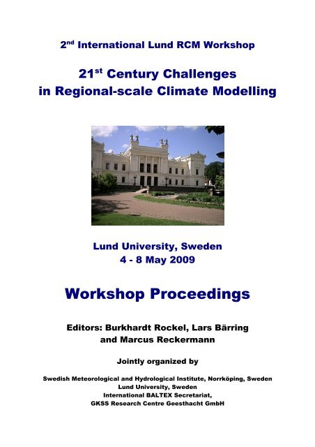
2 nd International Lund RCM Workshop<br />
21 st Century Challenges<br />
in Regional-scale Climate Modelling<br />
Lund University, Sweden<br />
4 - 8 May 2009<br />
Workshop Proceedings<br />
Editors: Burkhardt Rockel, Lars Bärring<br />
and Marcus Reckermann<br />
Jointly organized by<br />
Swedish Meteorological and Hydrological Institute, Norrköping, Sweden<br />
Lund University, Sweden<br />
International <strong>BALTEX</strong> Secretariat,<br />
GKSS Research Centre Geesthacht GmbH
Organisers and Sponsors<br />
Lund University<br />
Swedish Meteorological<br />
and Hydrological Institute<br />
GKSS Research Centre Geesthacht<br />
U.S. National Science Foundation<br />
World Climate Research Programme<br />
World Meteorological Organization<br />
Swedish Environmental Protection Agency<br />
Swedish Research Council for Environment
Associated Organisations<br />
ENSEMBLES<br />
North American Regional<br />
Climate Change Assessment Programme<br />
<strong>BALTEX</strong> – The Baltic Sea Experiment<br />
Global Energy and Water Cycle Experiment<br />
Danish Meteorological Institute
Scientific Committee<br />
Raymond Arritt, Iowa State University, USA<br />
Lars Bärring, Swedish Meteorological and Hydrological Institute and Lund University, Sweden<br />
Jens Hesselbjerg Christensen, Danish Meteorological Institute, Denmark<br />
Ole Bøssing Christensen, Danish Meteorological Institute, Denmark<br />
Michel Déqué, Météo-France, France<br />
Congbin Fu, Institute of Atmospheric Physics, Chinese Academy of Sciences, China<br />
Filippo Giorgi, Abdus Salam International Centre for Theoretical Physics, Italy<br />
Richard Jones, Met Office, U.K.<br />
Jack Katzfey, Centre for Australian Weather and Climate Research, Australia<br />
Rupa Kumar Kolli, World Meteorological Organization, Switzerland<br />
René Laprise, Université du Québec à Montréal, Canada<br />
Markus Meier, Swedish Meteorological and Hydrological Institute and Stockholm University, Sweden<br />
Claudio Menendez, Centro de Investigaciones del Mar y la Atmósfera, Argentina<br />
Roger Pielke Sr., University of Colorado, USA<br />
Burkhardt Rockel, GKSS Research Centre, Germany<br />
Markku Rummukainen, Swedish Meteorological and Hydrological Institute, Sweden<br />
Benjamin Smith, Lund University, Sweden<br />
Hans von Storch, GKSS Research Centre and University of Hamburg, Germany<br />
Organising Committee<br />
Lars Bärring, Swedish Meteorological and Hydrological Institute and Lund University, Sweden<br />
Ole Bøssing Christensen, Danish Meteorological Institute, Denmark<br />
Hans-Jörg Isemer, International <strong>BALTEX</strong> Secretariat, GKSS Research Centre, Germany<br />
Anna Maria Jönsson, Lund University, Sweden<br />
Marcus Reckermann, International <strong>BALTEX</strong> Secretariat, GKSS Research Centre, Germany<br />
Burkhardt Rockel, GKSS Research Centre, Germany
Preface<br />
This Second Lund Regional-scale Climate Modelling Workshop is a follow-up to the first regionalscale<br />
climate modelling workshop 1 held in Lund, Sweden in 2004. The overall theme of the first workshop<br />
was “High-resolution climate modelling: Assessment, added value and applications.” Now, five<br />
years later, it is again time to take stock of the scientific progress in the wide range of topics that<br />
regional climate modelling spans. These range from theoretical understanding and parameterisation of<br />
meso-scale and regional processes in the atmosphere/ocean/land surface/biosphere system, numerical<br />
methods and links between regional climate modelling and global climate/earth system models as well<br />
as numerical weather prediction models, evaluation of models using various observational datasets,<br />
model intercomparison and ensemble-based methods, production and utility of regional climate<br />
scenarios, and the application of regional climate modelling output for impact studies.<br />
This Second Lund Regional-scale Climate Modelling Workshop summarises developments and<br />
progress achieved in the last five years, discusses open issues and focuses on expected future<br />
challenges related to regional climate modelling. Thus, the overall theme for this workshop is 21st<br />
Century Challenges in Regional-scale Climate Modelling.<br />
The interest in this workshop was overwhelming. We received over 170 paper contributions from<br />
scientists all over the world; a total of about 220 participants from 43 countries registered for the<br />
workshop. As time is a tight resource in a 5-day workshop, many high-quality papers which were<br />
originally intended as oral presentations had to be realigned as posters. Therefore it is our policy not to<br />
distinguish between oral and poster presentations in this proceedings volume. It contains abstracts of<br />
all papers presented at the workshop, ordered alphabetically within sessions. Half a day of the<br />
workshop is dedicated to group and breakout sessions, some of which are open.<br />
The workshop is organised by the Swedish Meteorological and Hydrological Institute (SMHI), Lund<br />
University, the Danish Meteorological Institute (DMI) and GKSS-Forschungszentrum Geesthacht<br />
GmbH (GKSS), with support by the International <strong>BALTEX</strong> Secretariat. The scientific committee was<br />
responsible for preparing the workshop content and the scientific programme, while practical and<br />
logistic arrangements were managed by the organising committee (see preceding page).<br />
We are grateful for a generous endorsement by the following organisations: the World Meteorological<br />
Organization (WMO); the World Climate Research Programme (WCRP); the WCRP Global Energy<br />
and Water Cycle Experiment (GEWEX); the U.S. National Science Foundation (NSF); the<br />
ENSEMBLES project co-financed by EU FP-6; the North American Regional Climate Change<br />
Program (NARCCAP); the Swedish Research Council for Environment, Agricultural Sciences and<br />
Spatial Planning (Formas); the Swedish Environmental Protection Agency (Swedish EPA); and the<br />
GEWEX-CEOP Regional Hydroclimate Project <strong>BALTEX</strong> (Baltic Sea Experiment).<br />
This workshop brings together scientists from a wide range of disciplines that share a common interest<br />
in regional climate models. We hope that the interdisciplinary programme and the truly international<br />
group of participants will stimulate the exchange of views and discussions, and provide a fertile<br />
ground for future research directions and new collaborations.<br />
April 2009<br />
Burkhardt Rockel, Lars Bärring, and Marcus Reckermann<br />
Editors<br />
1 http://www.nateko.lu.se/Elibrary/LeRPG/5/LeRPG5Article.pdf
I<br />
Contents<br />
Session 1: Dynamical Downscaling<br />
Influence of large-scale nudging on regional climate model simulations<br />
Adelina Alexandru, Ramon de Elia, René Laprise, Leo Separovic and Sébastien Biner ............ 1<br />
A comparison of RCM performance for the eastern Baltic region and the application<br />
of the histogram equalization method for RCM outputs<br />
Uldis Bethers, Juris Seņņikovs and Andrejs Timuhins................................................................ 3<br />
Comparison of spatial filters and application to the ENSEMBLES regional climate<br />
model simulations<br />
Erasmo Buonomo and Richard Jones........................................................................................... 5<br />
Dynamical downscaling: Assessment of model system dependent retained and added<br />
variability for two different regional climate models<br />
Christopher L. Castro, Burkhardt Rockel, Roger A. Pielke Sr., Hans von Storch,<br />
and Giovanni Leoncini................................................................................................................. 6<br />
Improvement of long-term integrations by increasing RCM domain size<br />
Sin Chan Chou, André Lyra, José Pesquero, Lincoln Alves, Gustavo Sueiro, Diego Chagas,<br />
José Marengo and Vladimir Djurdjevic ....................................................................................... 8<br />
CLM coupled in the RegCM3 model: Preliminary results over South America<br />
Rosmeri P. da Rocha, Santiago V. Cuadra, Julio Pablo Reyes Fernandez<br />
and Allison L. Steiner .................................................................................................................. 9<br />
Assessment of dynamical downscaling in river basins in Japan using the Regional<br />
Atmospheric Modelling System (RAMS)<br />
Koji Dairaku, Satoshi Iizuka, Wataru Sasaki, Roger A. Pielke Sr. and Adriana Beltran .......... 11<br />
Sensitivity study of CRCM-simulated climate change projections<br />
Ramón De Elía and Hélène Côté................................................................................................ 12<br />
Regional precipitation anomalies in eastern Amazon as depicted by observations and<br />
REGCM3 simulations<br />
Everaldo B. De Souza, Marcio N. G. Lopes and Alan C. Cunha............................................... 14<br />
Assessment of precipitation as simulated by an RCM and its driving data<br />
Alejandro Di Luca, Ramón de Elía and René Laprise ............................................................... 16<br />
The Asian summer monsoon in ERA40 driven CLM simulations<br />
Andreas Dobler and Bodo Ahrens ............................................................................................. 18<br />
Added value of limited area model results<br />
Frauke Feser, Hans von Storch, Jörg Winterfeldt and Matthias Zahn ....................................... 20<br />
Sensitivity of CRCM basin annual runoff to driving data update frequency<br />
Anne Frigon and Michel Slivitzky............................................................................................. 22
II<br />
High-resolution dynamical downscaling error components over complex terrain<br />
Andreas Gobiet, M. Suklitsch, A. Prein, H. Truhetz, N.K. Awan, H. Goettel and D. Jacob..... 24<br />
Climate change projections for the XXI century over the Iberian peninsula using<br />
dynamic downscaling<br />
Juan José Gómez-Navarro, J.P. Montávez, S. Jerez and P. Jiménez-Guerrero.......................... 25<br />
Regional climate change scenarios – benefits of modelling in high resolution for central<br />
and eastern Europe in the project CECILIA<br />
Tomas Halenka, Michal Belda and Jiri Miksovsky ................................................................... 27<br />
Climatological feature and heating mechanism of the Foehn phenomena over the north<br />
of the central mountain range in Japan by using non-hydrostatic RCM<br />
Noriko Ishizaki and Izuru Takayabu.......................................................................................... 29<br />
Errors of interannual variability and multi-decadal trend in dynamical regional climate<br />
downscaling and their corrections<br />
Masao Kanamitsu, Kei Yoshimura, Yoo-Bin Yhang and Song-You Hong............................... 31<br />
Sensitivity of the simulated East Asian summer climatology to convective schemes<br />
using the NCEP regional spectral model<br />
Hyun-Suk Kang, Song-You Hong and Won-Tae Kwon............................................................ 33<br />
Study of climate change over the Caspian Sea basin using the climate model PRECIS<br />
at 2071-2100<br />
Maryam Karimian, Iman Babaeien and Rahele Modirian ......................................................... 35<br />
Performance of pattern scaling in estimating local changes for untried GCM-RCM<br />
pairs: Implications for ensemble design<br />
Elizabeth Kendon ....................................................................................................................... 36<br />
Evaluation of the analyzed large-scale features in a global data assimilation system<br />
due to different convective parameterization schemes and their impact on downscaled<br />
climatology using a RCM<br />
Jung-Eun Kim and Song-You Hong .......................................................................................... 38<br />
Sensitivity studies with a statistical downscaling method, the role of the driving large<br />
scale model<br />
Frank Kreienkamp, Arne Spekat and Wolfgang Enke............................................................... 40<br />
MPI regional climate model REMO simulations over South Asia<br />
Pankaj Kumar, Ralf Podzun and Daniela Jacob......................................................................... 41<br />
Settled and remaining issues in regional climate modelling with limited area nested<br />
models<br />
René Laprise, Ramón de Elia, Daniel Caya, Sébastien Biner, Philippe Lucas-Picher, Emilia<br />
Diaconescu, Martin Leduc, Adelina Alexandru, Leo Separovic and Alejandro di Luca........... 43<br />
Regional climate model skill to develop small-scale transient eddies<br />
Martin Leduc, René Laprise, Mathieu Moretti-Poisson and Jean-Philippe Morin .................... 45
III<br />
Evaluation of dynamical downscaling of the East Asian regional climate using the<br />
HadGEM3-RA: Summer monsoon of 1997 and 1998<br />
Johan Lee, Suhee Park, Wilfran Moufouma-Okia, David Hassell, Richard Jones,<br />
Hyun-Suk Kang, Young-Hwa Byun and Won-Tae Kwon......................................................... 47<br />
Interpolating temperature fields using static and dynamic lapse rates<br />
Chris Lennard............................................................................................................................. 49<br />
Regional modelling of climate and extremes in southeast China<br />
Laurent Li, Weilin Chen and Zhihong Jiang.............................................................................. 51<br />
Investigation of regional climate models’ internal variability with a ten-member<br />
ensemble of ten-year simulations over a large domain<br />
Philippe Lucas-Picher, Daniel Caya, Ramón de Elía, Sébastien Biner and René Laprise......... 52<br />
Selected examples of the added value of regional climate models<br />
H. E. Markus Meier, Lars Bärring, Ole Bössing Christensen, Erik Kjellström,<br />
Philip Lorenz, Burkhardt Rockel and Eduardo Zorita .............................................................. 54<br />
Climate change in Europe simulated by the regional climate model COSMO-CLM<br />
Kai S. Radtke and Klaus Keuler................................................................................................. 56<br />
Simulation of South Asian summer monsoon dynamics using REMO<br />
Fahad Saeed, Stefan Hagemann and Daniela Jacob................................................................... 58<br />
Analysis of precipitation changes in central Europe within the next decades based on<br />
simulations with a high resolution RCM ensemble<br />
Gerd Schädler, Hendrik Feldmann and Hans-Jürgen Panitz...................................................... 59<br />
Sensitivity studies of model setup in the alpine region using MM5 and RegCM<br />
Irene Schicker, Imran Nadeem and Herbert Formayer .............................................................. 61<br />
Parameter perturbation study with the GEM-LAM: The issue of domain size<br />
Leo Separovic, Ramon de Elia and René Laprise...................................................................... 63<br />
Modelling climate over Russian regions: RCM validation and projections<br />
Igor Shkolnik, S. Efimov, T. Pavlova and E. Nadyozhina......................................................... 65<br />
Is the position of the model domain over the target area related to the results of a<br />
regional climate model?<br />
Kevin Sieck, Philip Lorenz and Daniela Jacob .......................................................................... 66<br />
Estimating the Mediterranean Sea water budget: Impact of the design of the RCM<br />
Samuel Somot, Nellie Elguindi, Emilia Sanchez-Gomez, Marine Herrmann<br />
and Michel Déqué ...................................................................................................................... 67<br />
Comparison of climate change over Europe based on global and regional model<br />
Lidija Srnec, Mirta Patarčić and Čedo Branković...................................................................... 69
IV<br />
Investigation of added value at very high resolution with the regional climate model<br />
CCLM<br />
Martin Suklitsch and Andreas Gobiet ........................................................................................ 71<br />
A general approach for smoothing on a variable grid<br />
Dorina Surcel and René Laprise................................................................................................. 73<br />
What details can the regional climate models add to the global projections in the<br />
Carpathian Basin?<br />
Gabriella Szépszó, Gabriella Csima and András Horányi ......................................................... 75<br />
Investigation of precipitation over contiguous China using the Weather Research and<br />
Forecasting (WRF) model<br />
Jian Tang and Jianping Tang...................................................................................................... 76<br />
Impacts of the Spectral Nudging Technique on simulation of the East Asian summer<br />
monsoon in 1991<br />
Jianping Tang and Shi Song....................................................................................................... 78<br />
Extremes and predictability in the European pre-industrial climate of a regional climate<br />
model<br />
Lorenzo Tomassini, Ch. Moseley, A. Haumann, R. Podzun, and D. Jacob............................... 80<br />
Large-scale skill in regional climate modelling and the lateral boundary condition<br />
scheme<br />
Katarina Veljovic, Borivoj Rajkovic and Fedor Mesinger ........................................................ 82<br />
Does dynamical downscaling with regional atmospheric models add value to surface<br />
marine wind speed from re-analyses?<br />
Jörg Winterfeldt and Ralf Weisse .............................................................................................. 83<br />
Present climate simulations (1982-2003) of precipitation and surface temperature using<br />
the RegCM3, RSM and WRF<br />
Yoo-Bin Yhang, Kyo-Sun Lim, E-Hyung Park and Song-You Hong ....................................... 85<br />
Incremental interpolation of coarse global forcings for regional model integrations<br />
Kei Yoshimura and M. Kanamitsu............................................................................................. 87<br />
Development of a long-term climatology of North Atlantic polar lows using an RCM<br />
Matthias Zahn and Hans von Storch .......................................................................................... 89
V<br />
Session 2: New Developments in Numerics and Physical Parameterizations<br />
Examining the relative roles of precipitation and cloud material feedback generated by<br />
convective parameterization<br />
Christopher J. Anderson............................................................................................................. 91<br />
Dynamical coupling of the HIRHAM regional climate model and the MIKE SHE<br />
hydrological model<br />
Martin Drews, Søren H. Rasmussen, Jens Hesselbjerg Christensen, Michael B. Butts,<br />
Jesper Overgaard, Sara Maria Lerer and Jens Christian Refsgaard ........................................... 93<br />
A parameterization of aircraft induced cloudiness in the CLM regional climate model<br />
Andrew Ferrone, Philippe Marbaix, Ben Matthews, Ralph Lescroart<br />
and Jean-Pascal van Ypersele .................................................................................................... 95<br />
Stratospheric variability and its impact on surface climate<br />
Andreas Marc Fischer, Isla Simpson, Stefan Brönnimann, Eugene Rozanov<br />
and Martin Schraner................................................................................................................... 97<br />
Effects of numerical methods on high resolution modelling<br />
Holger Göttel.............................................................................................................................. 99<br />
Development of a climate model with dynamic grid streching<br />
William J. Gutowski Jr., Babatunde Abiodun, Joseph Prusa and Piotr Smolarkiewicz .......... 101<br />
Study of the capability of the RegCM3 in the simulation of precipitation and<br />
temperature over the Khorasan Razavi province, case study: Winters of 1991-2000<br />
Maryam Karimian, Iman Babeiean and Rahele Modirian ....................................................... 103<br />
Simulating aerosol effects on the dynamics and microphysics of precipitation systems<br />
with spectral bin and bulk parameterization schemes<br />
Lai-Yung Ruby Leung, Alexander P. Khain and Barry Lynn ................................................. 104<br />
Evaluation of the land surface scheme HTESSEL with satellite derived surface energy<br />
fluxes at the seasonal time scale<br />
Erik van Meijgaard, Louise Wipfler, Bart van den Hurk, Klaas Mestelaar, Jos van Dam,<br />
Reinder Feddes, Bert van Ulft, Sander Zwart and Wim Bastiaanssen..................................... 105<br />
Simulation of precipitation and temperature over the Khorasan province using Reg<br />
CM3, case study: Autumns 1991-2000<br />
Rahele Modirian, Iman Babaeian and Maryam Karimian...................................................................107<br />
Diffusion impact on atmospheric moisture transport<br />
Christopher Moseley, J. Haerter, H. Göttel, G. Zängl, S. Hagemann and D. Jacob ................ 108<br />
Climate simulations over North America with the Canadian Regional Climate Model<br />
(CRCM): From operational Version 4 to developmental Version 5<br />
Dominique Paquin, René Laprise, Katja Winger, Ramon de Elia, Ayrton Zadra<br />
and Bernard Dugas ................................................................................................................... 109
VI<br />
Soil organic layer: Implications for Arctic present-day climate and future climate<br />
changes<br />
Annette Rinke, Peter Kuhry and Klaus Dethloff...................................................................... 111<br />
Impact of surface waves in a regional climate model<br />
Anna Rutgersson, Björn Carlsson, Alvaro Semedo and Øyvind Sætra ................................... 112<br />
Sensitivity of a regional climate model to physics parameterizations: Simulation of<br />
summer precipitation over East Asia using MM5<br />
Shi Song and Jianping Tang..................................................................................................... 114<br />
Overview over recent developments of COSMO-CLM numerics and physical<br />
parameterizations for high resolution simulations<br />
Andreas Will and Ulrich Schättler ........................................................................................... 116<br />
Evaluation of the Rossby Centre regional climate model (RCA) using satellite cloud and<br />
radiation products<br />
Ulrika Willen............................................................................................................................ 117<br />
Simulating aerosols in the regional climate model CCLM<br />
Elias Zubler, Ulrike Lohmann, Daniel Lüthi, Andreas Mühlbauer and Christoph Schär........ 119<br />
Session 3: From Weather to Climate<br />
Moisture availability and the relationship between daily precipitation intensity and<br />
surface temperature<br />
Peter Berg, Jan Haerter, Peter Thejll, Claudio Piani, Stefan Hagemann<br />
and Jens Hesselbjerg Christensen ............................................................................................ 121<br />
Temperature and precipitation scenarios for the Caribbean from the PRECIS regional<br />
climate model<br />
Jayaka Campbell, M. A. Taylor, T. S. Stephenson, F. S. Whyte and R. Watson .................... 123<br />
Use of the Weather Research and Forecasting Model (WRF): Towards improving warm<br />
season climate forecasts in North America<br />
Christopher L. Castro and Francina Dominguez...................................................................... 124<br />
Modelling of the Atlantic tropical cyclone activity with the RegCM3<br />
Daniela Cruz-Pastrana, Ernesto Caetano and Rosmeri Porfírio da Rocha............................... 126<br />
Regional modelling of recent changes in the climate of Svalbard and the Nordic Arctic<br />
(1979-2001): Comparing RCM output to meteorological station data<br />
Jonathan Day, Jonathan Bamber, Paul Valdes and Jack Kohler.............................................. 128<br />
Effects of variations in climate parameters on evapotranspiration in the arid<br />
and semi-arid regions<br />
Saeid Eslamian, Mohammad Javad Khordadi, Arezou Baba Ahmadi<br />
and Jahangir Abedi Koupai ...................................................................................................... 129
VII<br />
Regional climate change projections using a physics ensemble over the Iberian<br />
Peninsula<br />
Pedro Jiménez Guerrero, S. Jerez, J.P. Montavez, J.J. Gomez-Navarro, J.A. García-Valero<br />
and J.F. Gonzalez-Rouco ......................................................................................................... 130<br />
Effect of internal variability on regional climate change projections<br />
Klaus Keuler, Kai Radtke and Andreas Will ........................................................................... 132<br />
An ensemble of regional climate change simulations<br />
Erik Kjellström, Grigory Nikulin, Lars Bärring, Ulf Hansson, Gustav Strandberg<br />
and Anders Ullerstig................................................................................................................. 134<br />
Detailed assessment of climate variability of the Baltic Sea for the period 1950/70-2008<br />
Andreas Lehmann, Klaus Getzlaff, Jan Harlass and Karl Bumke ........................................... 136<br />
Diurnal variation of precipitation over central eastern China simulated by a regional<br />
climate model (CREM)<br />
Jian Li, Rucong Yu, Tianjun Zhou, Wei Huang and Hongbo Shi ........................................... 138<br />
Investigation of ‘Hurricane Katrina’ type characteristics for future, warmer climates<br />
Barry H. Lynn, Richard J. Healy and Leonard Druyan............................................................ 139<br />
Evaluation of seasonal forecasts over the northeast of Brazil using the RegCM3<br />
Rubinei Dorneles Machado and Rosmeri Porfírio da Rocha ................................................... 141<br />
An evaluation of surface radiation budget over North America in a suite of regional<br />
climate models<br />
Marko Markovic, C.G. Jones, P.Vaillancourt, K.Winger and D.Paquin ................................. 144<br />
Climate change assessment over Iran during future decades by using the MAGICC-<br />
SCENGEN model<br />
Majid Habibi Nokhandan, Fatemeh Abassi, Azade Goli Mokhtari and Iman Babaeian ......... 145<br />
Dynamical downscaling of ECMWF experimental seasonal forecasts: Probabilistic<br />
verification<br />
Mirta Patarčić and Čedo Branković ......................................................................................... 146<br />
Cut-off <strong>Low</strong> Systems: Comparison NCEP versus RegCM3<br />
Michelle Simoes Reboita, Raquel Nieto, Luis Gimeno, Rosmeri Porfirio da Rocha<br />
and Tercio Ambrizzi................................................................................................................. 148<br />
Relative role of domain size, grid size, and initial conditions in the simulation of high<br />
impact weather events<br />
Himesh Shivappa, P .Goswami and B.S. Goud ....................................................................... 150<br />
Weighting multi-models in seasonal forecasting – and what can be learnt for the<br />
combination of RCMs<br />
Andreas P. Weigel, Mark A. Liniger and C. Appenzeller ....................................................... 152
VIII<br />
Session 4: Regional Observational Data and Reanalysis<br />
High-resolution simulation of a windstorm event to assess sampling characteristics of<br />
windstorm measures based on observations<br />
Lars Bärring, Włodzimierz Pawlak, Krzysztof Fortuniak and Ulf Andrae.............................. 155<br />
MesoClim – A mesoscale alpine climatology using VERA-reanalyses<br />
Benedikt Bica, Stefan Sperka and Reinhold Steinacker .......................................................... 157<br />
Observed and modeled extremes indices in the CECILIA project<br />
Ole B. Christensen, Fredrik Boberg, Martin Hirschi, Sonia Seneviratne and Petr Stepanek .. 159<br />
Dynamical downscaling of surface wind circulations over complex terrain<br />
Pedro A. Jiménez, J. Fidel González-Rouco, Juan P. Montávez, E. García-Bustamante<br />
and J. Navarro .......................................................................................................................... 160<br />
JP10: 59-year 10 km dynamical downscaling of reanalysis over Japan<br />
Hideki Kanamaru, Kei Yoshimura, Wataru Ohfuchi, Kozo Ninomiya<br />
and Masao Kanamitsu .............................................................................................................. 162<br />
Satellite-based datasets for validation of regional climate models: The CM-SAF product<br />
suite and new possibilities for processing with 'climate data operators'<br />
Frank Kaspar, J. Schulz, P. Fuchs, R. Hollmann, M. Schröder, R. Müller, K.-G. Karlsson,<br />
R. Roebeling, A. Riihelä, B. de Paepe, R. Stöckli and U. Schulzweida ................................. 164<br />
Reflection of shifts in upper-air wind regime in surface meteorological parameters in<br />
Estonia during recent decades<br />
Sirje Keevallik and Tarmo Soomere ........................................................................................ 166<br />
Regional features of recent climate change in Europe: The aggregated index approach<br />
Valeriy Khokhlov and Lyndmila G. Latysh............................................................................. 168<br />
Hindcasting Europe’s climate – A user perspective<br />
Thomas Klein ........................................................................................................................... 170<br />
Analysis of surface air temperatures over Ireland from re-analysis Data and<br />
observational Data<br />
Priscilla A. Mooney, Frank J. Mulligan and Rowan Fealy...................................................... 171<br />
Environment database and the Geographic Information System for socio-economic<br />
planning<br />
Olakunle Francis Omidiora and Balogun Ahmed .................................................................... 173<br />
The AMMA field campaign and its potential for model validation<br />
Jan Polcher and the AMMA partners....................................................................................... 174<br />
Climate change and water pollution interactions in the Republic of Belarus<br />
Veranika Selitskaya and Alena Kamarouskaya ....................................................................... 175<br />
Current-climate downscaling of winds and precipitation for the eastern Mediterranean<br />
Scott Swerdlin, Thomas Warner, Andrea Hahmann, Dorita Rostkier-Edelstein<br />
and Yubao Liu.......................................................................................................................... 176
IX<br />
Current climate downscaling at the National Center for Atmospheric Research (NCAR)<br />
Thomas Warner, Scott Swerdlin, Yubao Liu and Daran Rife.................................................. 178<br />
Session 5: Results from Large Projects<br />
Verification of simulated near surface wind speeds by a multi model ensemble with<br />
focus on coastal regions<br />
Ivonne Anders, Hans von Storch and Burkhardt Rockel ......................................................... 181<br />
The North American Regional Climate Change Assessment Program (NARCCAP):<br />
Status and results<br />
Raymond W. Arritt................................................................................................................... 183<br />
MRED: Multi-RCM ensemble downscaling of global seasonal forecasts<br />
Raymond W. Arritt................................................................................................................... 184<br />
An atmosphere-ocean regional climate model for the Mediterranean area: Present<br />
climate and XXI scenario simulations<br />
V. Artale, S. Calmanti, A. Carillo, A. Dell’Aquila, M. Herrmann, G. Pisacane, PM Ruti,<br />
G. Sannino, MV Struglia, F. Giorgi, X. Bi, J.S. Pal and S. Rauscher ..................................... 185<br />
Regional climate modelling in Morocco within the project IMPETUS Westafrica<br />
Kai Born, H. Paeth, K. Piecha, and A. H. Fink........................................................................ 186<br />
Will future summer time temperatures go berserk?<br />
Jens H. Christensen, Fredrik Boberg, Philippe Lucas-Picher and Ole B. Christensen ............ 188<br />
An atmosphere-ocean coupled model for the Mediterranean climate simulation<br />
Alberto Elizalde, Daniela Jacob and Uwe Mikolajewicz......................................................... 190<br />
Inter-comparison of Asian monsoon simulated by RCMs in Phase II of RMIP for Asia<br />
Jinming Feng, Congbin Fu, Shuyu Wang, Jianping Tang, D. Lee, Y. Sato, H. Kato<br />
and J. McGregor....................................................................................................................... 191<br />
From droughts to floods: A statistical assessment from RCM<br />
Sandra G. Garcia and J.D. Giraldo........................................................................................... 192<br />
On the validation of RCMs in terms of reproducing the annual cycle<br />
Tomas Halenka, Petr Skalak and Michal Belda....................................................................... 193<br />
AMMA-Model Intercomparison Project<br />
F. Hourdin, J. Polcher, F. Guichard, F. Favot, J.P. Lafore, J.L. Redelsperger, Ruti PM, A.<br />
Dell'Aquila, T. Losada and A.K. Traoer ................................................................................. 195<br />
Projection of the changes in the future extremes over Japan using a cloud-resolving<br />
model (JMA-NHM): Change in heavy precipitation<br />
Sachie Kanada, M. Nakano, M. Nakamura, S. Hayashi, T. Kato, H. Sasaki, T. Uchiyama, K.<br />
Aranami, Y. Honda, K. Kurihara and A. Kitoh ....................................................................... 196
X<br />
Predicting water resources in West Africa for 2050<br />
Harouna Karambiri, S. Garcia, H. Adamou, L. Decroix, A. Mariko, S. Sambou<br />
and E. Vissin ............................................................................................................................ 198<br />
Evaluation of European snow cover as simulated by an ensemble of regional climate<br />
models<br />
Sven Kotlarski, Daniel Lüthi and Christoph Schär .................................................................. 199<br />
Projections of the eastern Mediterranean climate change simulated in a transient RCM<br />
experiment with RegCM3<br />
Simon Krichak, Pinhas Alpert and Pavel Kunin...................................................................... 201<br />
Atmospheric river induced heavy precipitation and flooding in the NARCCAP<br />
simulations<br />
Lai-Yung Ruby Leung and Yun Qian...................................................................................... 203<br />
Intra-seasonal evolution of the West African monsoon: Results from multiple RCM<br />
simulations<br />
Neil MacKellar, Philippe Lucas-Picher, Jens H. Christensen and Ole B. Christensen............ 204<br />
CLARIS Project: Towards climate downscaling in South America using RCA3<br />
Claudio G. Menéndez, Anna Sörensson, Patrick Samuelsson, Ulrika Willén, Ulf Hansson,<br />
Manuel de Castro and Jean-Philippe Boulanger ...................................................................... 205<br />
Influence of soil moisture initialization on regional climate model simulations of the<br />
West African monsoon<br />
Wilfran Moufouma-Okia and Dave Rowell............................................................................. 207<br />
Projection of the changes in the future extremes over Japan using a cloud-resolving<br />
model (JMA-NHM): Model verification and first results<br />
Masuo Nakano, S. Kanada, M. Nakamura, S. Hayashi, T. Kato, H. Sasaki, T. Uchiyama,<br />
K. Aranami, Y. Honda, K. Kurihara and A. Kitoh................................................................... 209<br />
Regional climate model studies in CEOP: The Inter-Continental Transferability Study<br />
(ICTS)<br />
Burkhardt Rockel, Beate Geyer, William J. Gutowski Jr., C.G. Jones, Z. Kodhavala,<br />
I. Meinke, D. Paquin and A. Zadra .......................................................................................... 211<br />
ENSEMBLES regional climate model simulations for Western Africa (the “AMMA”<br />
region)<br />
Markku Rummukainen, Filippo Giorgi and the ENSEMBLES RT3 participants................... 213<br />
Assessing the performance of seasonal snow in the NARCCAP RCMs – An analyses for<br />
the upper Colorado river basin<br />
Nadine Salzmann and Linda Mearns ....................................................................................... 215<br />
Applying the Rossby Centre regional climate model (RCA3.5) over the ENSEMBLES-<br />
AMMA region: Sensitivity studies and future scenarios<br />
Patrick Samuelsson, Ulrika Willén, Erik Kjellström and Colin Jones..................................... 217
XI<br />
Interactions between European shelves and the Atlantic simulated with a coupled<br />
regional atmosphere-ocean-biogeochemistry model<br />
Dmitry V. Sein, Joachim Segschneider, Uwe Mikolajewicz and Ernst Maier-Reimer ........... 219<br />
ALADIN-Climate/CZ simulation of the 21 st century climate in the Czech Republic for<br />
the A1B emission scenario<br />
Petr Skalak, Petr Stepanek and Ales Farda .............................................................................. 221<br />
Overview of the research project of multi-model ensembles and down-scaling methods<br />
for assessment of climate change impact, supported by MoE Japan<br />
Izuru Takayabu......................................................................................................................... 222<br />
Simulation of Asian monsoon climate by RMIP Models<br />
Shuyu Wang, Jinming Feng, Zhe Xiong and Congbing Fu ..................................................... 224<br />
Session 6: The Future of RCMs<br />
Use of regional climate models in regional attribution studies<br />
Christopher J. Anderson, William J. Gutowski, Jr., Martin P. Hoerling<br />
and Xiaowei Quan.................................................................................................................... 227<br />
Wave estimations using winds from RCA, the Rossby regional climate model<br />
Barry Broman and Ekaterini E. Kriezi ..................................................................................... 229<br />
Development of a Regional Arctic Climate System Model (RACM)<br />
John Cassano, Wieslaw Maslowski, William Gutowski and Dennis Lettenmeier ................. 230<br />
Regional climate simulation with mosaic GCMs<br />
Michel Déqué ........................................................................................................................... 232<br />
A coupled regional climate model as a tool for understanding and improving feedback<br />
processes in Arctic climate simulations<br />
Wolfgang Dorn, Klaus Dethloff and Annette Rinke ............................................................... 233<br />
Arctic regional coupled downscaling of recent and possible future climates<br />
Ralf Döscher, T. Königk, K. Wyser, H. E. Markus Meier and P. Pemberton ......................... 235<br />
A regionally coupled atmosphere-ocean and sea ice model of the Arctic<br />
Ksenia Glushak, Dmitry Sein and Uwe Mikolajewicz ............................................................ 236<br />
Convection-resolving regional climate modelling and extreme event statistics for recent<br />
and future summer climate<br />
Christoph Knote, Günther Heinemann and Burkhardt Rockel ................................................ 237<br />
Numerical modelling of trace species cycles in regional climate model systems<br />
Baerbel Langmann ................................................................................................................... 238
XII<br />
The impact of atmospheric thermodynamics on local climate change predictability:<br />
A plea for very high resolution climate modelling<br />
Geert Lenderink and E. van Meijgaard .................................................................................... 240<br />
Chances of the global-regional two-way nesting approach<br />
Philip Lorenz and Daniela Jacob.............................................................................................. 242<br />
Very high-resolution regional climate simulations over Greenland with the HIRHAM<br />
model<br />
Philippe Lucas-Picher, Jens H. Christensen, Martin Stendel and Gudfinna Aðalgeirsdóttir... 243<br />
Time invariant input parameter processing for applications in the COSMO-CLM Model<br />
Gerhard Smiatek, Goran Georgievski and Hermann Asensio.................................................. 244<br />
Impact of convective parameterization on high resolution precipitation climatology<br />
using WRF for Indian summer monsoon<br />
Sourav Taraphdar, P. Mukhopadhyay, B. N. Goswami and K. Krishnakumar ....................... 245<br />
Development of a regional ocean-atmosphere coupled model and its performance in<br />
simulating the western North Pacific Summer monsoon<br />
Liwei Zou, Tianjun Zhou and Rucong Yu ............................................................................... 247<br />
Session 7: Impact Studies<br />
Regional climate change impact studies in the upper Danube and upper Brahmaputra<br />
river basin using CLM projections<br />
Bodo Ahrens and Andreas Dobler ........................................................................................... 249<br />
River runoff projection of future climate in Latvia<br />
Elga Apsīte, Anda Bakute and Līga Kurpniece ....................................................................... 251<br />
Application of regional-scale climate modelling to account for climate change in the<br />
hydrological design for dam safety in Sweden<br />
Sten Bergström, Johan Andréasson and L. Phil Graham ......................................................... 253<br />
Local air mass dependence of extreme temperature minima in the Gstettneralm<br />
Sinkhole with regard to global climate change<br />
Benedikt Bica and Reinhold Steinacker................................................................................... 255<br />
Impact of vegetation on the simulation of seasonal Monsoon rainfall over the Indian<br />
region using a regional model<br />
Surya Kanti Dutta, Someshwar Das, S.C. Kar, V.S. Prasad and Prasanta Mali ...................... 257<br />
Climate change impacts on the water quality: A case study of the Rosetta Branch in the<br />
Nile Delta, Egypt<br />
Alaa El-Sadek........................................................................................................................... 259<br />
Direct radiative forcing of various aerosol species over East Asia with a coupled regional<br />
climate/chemistry model<br />
Zhiwei Han............................................................................................................................... 260
XIII<br />
Influence of soil moisture near-surface temperature feedback on present and future<br />
climate simulations over the Iberian peninsula<br />
Sonia Jerez, J.P. Montavez, P. Jimenez-Guerrero, J.J. Gomez-Navarro<br />
and J.F. Gonzalez-Rouco ......................................................................................................... 261<br />
Forest damage in a changing climate<br />
Anna Maria Jönsson and Lars Bärring..................................................................................... 263<br />
Climate change and air pollution interactions in the Republic of Belarus<br />
Alena Kamarouskaya and Aliksandr Behanski........................................................................ 264<br />
Future challenges for regional coupled climate and environmental modelling in the<br />
Baltic Sea region<br />
H. E. Markus Meier, Thorsten Blenckner, Boris Chubarenko, Anna Gårdmark, Bo G.<br />
Gustafsson, Jonathan Havenhand, Brian MacKenzie, Björn-Ola Linnér, Thomas Neumann,<br />
Urmas Raudsepp, Tuija Ruoho-Airola, Jan-Marcin Weslawski and Eduardo Zorita.............. 265<br />
Linking climate factors and adaptation strategies in the rural Sahel-Sudan zone of West<br />
Africa<br />
Ole Mertz, Cheikh Mbow , Jonas Ø. Nielsen, Abdou Maiga, Alioune Ka, Rissa Diallo,<br />
Pierre Cissé, Drissa Coulibaly, Bruno Barbier, Dapola Da, Tanga Pierre Zoungrana,<br />
Ibrahim Bouzou Moussa, Waziri Mato Maman, Boureima Amadou, Addo Mahaman,<br />
Alio Mahaman, Amadou Oumarou, Daniel Dabi, Vincent Ihemegbulem, Awa Diouf,<br />
Malick Zoromé, Ibrahim Ouattara, Mamadou Kabré, Anette Reenberg, Kjeld Rasmussen<br />
and Inge Sandholt..................................................................................................................... 267<br />
Projected changes in daily temperature variability over Europe in an ensemble of RCM<br />
simulations<br />
Grigory Nikulin, Erik Kjellström and Lars Bärring................................................................. 268<br />
Climate change impact assessment in central and eastern Europe: The CLAVIER<br />
project<br />
Susanne Pfeifer, Daniela Jacob, Gabor Balint, Dan Balteanu, Andreas Gobiet, Andras<br />
Horanyi, Laurent Li, Franz Prettenthaler, Tamas Palvolgyi and Gabriella Szépszó................ 270<br />
Climate change impacts on extreme wind speeds<br />
Sara C. Pryor, R.J. Barthelmie, N.E. Claussen, N.M. Nielsen, E. Kjellström and M. Drews . 271<br />
Winter storms with high loss potential in a changing climate from a regional point of<br />
view<br />
Monika Rauthe, Michael Kunz and Susanna Mohr ................................................................. 273<br />
The impact of land use change at ShanGanNing border areas on climate with RegCM3<br />
Study<br />
Xueli Shi, Yiming Liu and Jianping Liu.................................................................................. 275<br />
Numerical investigations into the impact of urbanization on tropical mesoscale events<br />
Himesh Shivappa, P. Goswami and B.S. Goud ....................................................................... 276
XIV<br />
Observation and simulation with RegCM3 for the 2005-2006 rainy season over the<br />
southeast of Brazil<br />
Maria Elisa Siqueira Silva and Diogo Ladvocat Negrão Couto............................................... 278<br />
Simulating cold palaeo-climate conditions in Europe with a regional climate model<br />
Gustav Strandberg, Jenny Brandefelt, Erik Kjellström and Benjamin Smith.......................... 280<br />
Coupling climate and crop models<br />
Benjamin Sultan, A. Alhassane, P. Oettli, S. Traoré, C. Baron, B. Muller, M. Dingkuhn ...... 282<br />
Streamflow in the upper Mississippi river basin as simulated by SWAT driven<br />
by 20C results of NARCCAP regional climate models<br />
Eugene S. Takle, M. Jha, E. Lu, R.W. Arritt , W. J. Gutowski, Jr.<br />
and the NARCCAP Team ........................................................................................................ 283<br />
Dynamical downscaling of urban climate using CReSiBUC with inclusion of detailed<br />
land surface parameters<br />
Kenji Tanaka, Kazuyoshi Souma, Takahiro Fujii and Makoto Yamauchi .............................. 285<br />
Impact of megacities on the regional air quality: A South American case study<br />
Claas Teichmann and Daniela Jacob........................................................................................ 288<br />
Validation of RCM simulations using a conceptual runoff model<br />
Claudia Teutschbein and Jan Seibert ....................................................................................... 290<br />
Impacts of vegetation on the global water and energy budget as represented by the<br />
Community Atmosphere Model (CAM3)<br />
Zhongfeng Xu and Congbin Fu................................................................................................ 291
XV<br />
Index of Authors<br />
Abassi F. ............................................................145<br />
Abiodun B..........................................................101<br />
Aðalgeirsdóttir G................................................243<br />
Adamou H..........................................................198<br />
Ahrens B ......................................................18, 249<br />
Alexandru A.....................................................1, 43<br />
Alhassane A .......................................................284<br />
Alioune KA........................................................267<br />
Alpert P ..............................................................201<br />
Alves L...................................................................8<br />
Amadou B ..........................................................267<br />
Ambrizzi T.........................................................148<br />
Anders I..............................................................181<br />
Anderson CJ.................................................91, 227<br />
Andrae U............................................................155<br />
Andréasson J ......................................................253<br />
Appenzeller C ....................................................152<br />
Apsīte E..............................................................251<br />
Aranami K..................................................196, 209<br />
Arritt RW ...........................................183, 184, 283<br />
Artale V..............................................................185<br />
Asensio H...........................................................244<br />
Awan NK .............................................................24<br />
Baba Ahmadi A..................................................129<br />
Babaeian I ..................................................107, 145<br />
Bakute A ............................................................251<br />
Balint G..............................................................270<br />
Balogun A ..........................................................173<br />
Balteanu D .........................................................270<br />
Bamber J ............................................................128<br />
Barbier B............................................................267<br />
Baron C ..............................................................282<br />
Bärring L.............................. 54, 134, 155, 263, 268<br />
Barthelmie RJ.....................................................271<br />
Bastiaanssen W ..................................................105<br />
Behanski A.........................................................264<br />
Belda M........................................................27, 193<br />
Beltran-Przekurat A .............................................11<br />
Berg P ................................................................121<br />
Bergström S .......................................................253<br />
Bethers U ...............................................................3<br />
Bi X....................................................................185<br />
Bica B ........................................................159, 255<br />
Biner S .......................................................1, 43, 52<br />
Blenckner T........................................................265<br />
Boberg F.....................................................159, 188<br />
Born K................................................................186<br />
Boulanger J-P.....................................................205<br />
Bouzou Moussa I ...............................................267<br />
Brandefelt J ........................................................280<br />
Branković Č .................................................69, 182<br />
Broman B...........................................................229<br />
Brönnimann S ......................................................97<br />
Bumke K ............................................................136<br />
Buonomo E ...........................................................5<br />
Butts MB..............................................................93<br />
Byun Y-H.............................................................47<br />
Caetano E...........................................................126<br />
Calmanti S..........................................................185<br />
Campbell J .........................................................123<br />
Carillo A ............................................................185<br />
Carlsson B..........................................................112<br />
Cassano J............................................................230<br />
Castro CL.......................................................6, 124<br />
Caya D ...........................................................43, 52<br />
Chagas D................................................................8<br />
Chen W ...............................................................51<br />
Chou SC.................................................................8<br />
Christensen JH ..................... 93, 121, 190, 204, 243<br />
Christensen OB ............................54, 159, 188, 204<br />
Chubarenko B ....................................................265<br />
Cissé P................................................................267<br />
Claussen NE.......................................................271<br />
Colin J................................................................217<br />
Côté H..................................................................12<br />
Coulibaly D........................................................267<br />
Cruz-Pastrana D .................................................126<br />
Csima G ...............................................................75<br />
Cuadra SV..............................................................9<br />
Cunha AC.............................................................14<br />
Da D...................................................................267<br />
da Rocha RP...................................9, 126, 141, 148<br />
Dabi D................................................................267<br />
Dairaku K.............................................................11<br />
Das S..................................................................257<br />
Day J ..................................................................128<br />
de Castro M........................................................205<br />
de Elia R........................... 1, 12, 16, 43, 52, 63, 109<br />
de Paepe B..........................................................164<br />
de Souza EB.........................................................14<br />
Decroix L ...........................................................198<br />
Dell’Aquila A.............................................185, 195<br />
Déqué M ......................................................67, 232<br />
Dethloff K ..................................................111, 236<br />
di Luca A .......................................................16, 43<br />
Diaconescu E .......................................................43<br />
Diallo R..............................................................267<br />
Dingkuhn M.......................................................282<br />
Diouf A ..............................................................267<br />
Djurdjevic V...........................................................8<br />
Dobler A ......................................................18, 249<br />
Dominguez F......................................................124<br />
Dorn W ..............................................................233<br />
Döscher R...........................................................235<br />
Drews M ......................................................93, 271<br />
Dugas B..............................................................109<br />
Dutta SK ............................................................257<br />
Efimov S ..............................................................65<br />
Elguindi N............................................................67<br />
Elizalde A...........................................................190<br />
El-Sadek A.........................................................259<br />
Enke W ................................................................40<br />
Eslamian S .........................................................129<br />
Farda A ..............................................................221
XVI<br />
Favot F ...............................................................195<br />
Fealy R...............................................................171<br />
Feddes R.............................................................105<br />
Feldmann H..........................................................59<br />
Feng J.........................................................191, 224<br />
Ferrone A .............................................................95<br />
Feser F..................................................................20<br />
Fink AH .............................................................186<br />
Fischer AM ..........................................................97<br />
Formayer H ..........................................................61<br />
Fortuniak K ........................................................155<br />
Frigon A...............................................................22<br />
Fu C....................................................191, 224, 291<br />
Fuchs P ..............................................................164<br />
Fujii T ................................................................285<br />
Garcia S..............................................................198<br />
Garcia SG...........................................................192<br />
García-Bustamante E .........................................160<br />
García-Valero JA ...............................................130<br />
Gårdmark A .......................................................265<br />
Georgievski G ....................................................244<br />
Getzlaff K...........................................................136<br />
Geyer B ..............................................................211<br />
Gimeno L ...........................................................148<br />
Giorgi F......................................................185, 213<br />
Giraldo JD..........................................................192<br />
Glushak K ..........................................................236<br />
Gobiet A.................................................24, 71, 270<br />
Gomez-Navarro JJ................................25, 130, 261<br />
Gonzalez-Rouco JF............................130, 161, 261<br />
Goswami P.................................................150, 276<br />
Goswami BN......................................................245<br />
Göttel H..................................................24, 99, 108<br />
Goud BS.....................................................150, 276<br />
Graham LP.........................................................253<br />
Guichard F .........................................................195<br />
Gustafsson BG ...................................................265<br />
Gutowski Jr WJ.................. 101, 211, 227, 230, 283<br />
Haerter J.....................................................108, 121<br />
Hagemann S.........................................58, 108, 121<br />
Hahmann A ........................................................176<br />
Halenka T.....................................................27, 193<br />
Han Z .................................................................260<br />
Hansson U..................................................134, 205<br />
Harlass J.............................................................136<br />
Hassell D..............................................................45<br />
Haumann A ..........................................................80<br />
Havenhand J.......................................................265<br />
Hayashi S ...................................................196, 209<br />
Healy RJ.............................................................139<br />
Heinemann G .....................................................237<br />
Herrmann M.................................................67, 185<br />
Hirschi M ...........................................................159<br />
Hoerling MP.......................................................227<br />
Hollmann R........................................................164<br />
Honda Y.....................................................196, 209<br />
Hong S-Y ...........................................31, 33, 38, 85<br />
Horányi A.....................................................75, 270<br />
Hourdin F...........................................................195<br />
Huang W ............................................................138<br />
Ihemegbulem V..................................................267<br />
Iizuka S ................................................................11<br />
Ishizaki N.............................................................29<br />
Jacob D 24, 41, 58, 66, 80, 108, 190, 242, 270, 288<br />
Jerez S..................................................25, 130, 261<br />
Jha M..................................................................283<br />
Jiang Z..................................................................51<br />
Jiménez PA ........................................................160<br />
Jimenez-Guerrero P..............................25, 130, 261<br />
Jones CG ............................................144, 211, 217<br />
Jones R.............................................................5, 47<br />
Jönsson AM .......................................................263<br />
Ka A...................................................................267<br />
Kabré M .............................................................267<br />
Kamarouskaya A........................................175, 264<br />
Kanada S ....................................................196, 209<br />
Kanamaru H.......................................................162<br />
Kanamitsu M..........................................31, 87, 162<br />
Kang H-S .......................................................33, 47<br />
Kar SC................................................................257<br />
Karambiri H .......................................................198<br />
Karimian M..........................................35, 103, 107<br />
Karlsson K-G ....................................................164<br />
Kaspar F.............................................................164<br />
Kato H ...............................................................191<br />
Kato T ........................................................196, 209<br />
Keevallik S.........................................................166<br />
Kendon E .............................................................36<br />
Keuler K.......................................................56, 132<br />
Khain AP............................................................104<br />
Khokhlov V........................................................168<br />
Khordadi MJ ......................................................129<br />
Kim J-E ................................................................38<br />
Kitoh A ......................................................196, 209<br />
Kjellström E................. 54, 134, 217, 268, 271, 280<br />
Klein T ...............................................................170<br />
Knote C. .............................................................237<br />
Kodhavala Z.......................................................211<br />
Kohler J..............................................................128<br />
Königk T ............................................................235<br />
Kotlarski S .........................................................199<br />
Koupai JA ..........................................................129<br />
Kreienkamp F.......................................................40<br />
Krichak S ...........................................................201<br />
Kriezi EE............................................................229<br />
Krishnakumar K.................................................245<br />
Kuhry P..............................................................111<br />
Kumar P ...............................................................41<br />
Kunin P ..............................................................201<br />
Kunz M. .............................................................273<br />
Kurihara K .................................................196, 209<br />
Kurpniece L .......................................................251<br />
Kwon W-T .....................................................33, 47<br />
Lafore J-P...........................................................195<br />
Langmann B.......................................................238<br />
Laprise R.................... 1, 16, 43, 45, 52, 63, 73, 109<br />
Latysh LG ..........................................................168<br />
Leduc M.........................................................43, 45<br />
Lee D..................................................................191<br />
Lee J.....................................................................47<br />
Lehmann A.........................................................136<br />
Lenderink G .......................................................240<br />
Lennard C.............................................................49<br />
Leoncini G .............................................................6
XVII<br />
Lerer SM ..............................................................93<br />
Lescroart R...........................................................95<br />
Lettenmeier D ....................................................230<br />
Leung L-Y R..............................................104, 203<br />
Li J .....................................................................138<br />
Li L ..............................................................51, 270<br />
Lim K-S ...............................................................85<br />
Liniger MA ........................................................152<br />
Linnér B-O.........................................................265<br />
Liu J ...................................................................275<br />
Liu Y ..................................................176, 178, 275<br />
Lohmann U ........................................................119<br />
Lopes MNG .........................................................14<br />
Lorenz P.................................................54, 66, 242<br />
Losada T.............................................................195<br />
Lu E....................................................................283<br />
Lucas-Picher P .......................43, 52, 188, 204, 243<br />
Lüthi D.......................................................119, 199<br />
Lynn B .......................................................102, 139<br />
Lyra A ....................................................................8<br />
Machado RD ......................................................141<br />
MacKellar N.......................................................204<br />
MacKenzie B .....................................................265<br />
Mahaman A........................................................267<br />
Maier-Reimer E .................................................219<br />
Maiga A .............................................................267<br />
Mali P.................................................................257<br />
Marbaix P.............................................................95<br />
Marengo J...............................................................8<br />
Mariko A............................................................198<br />
Markovic M .......................................................144<br />
Maslowski M .....................................................230<br />
Mato-Maman W.................................................267<br />
Matthews B ..........................................................95<br />
Mbow C .............................................................267<br />
McGregor J ........................................................191<br />
Mearns L ............................................................215<br />
Meier MHE .........................................54, 235, 265<br />
Meinke I ............................................................211<br />
Menéndez CG ....................................................205<br />
Mertz O ..............................................................267<br />
Mesinger F ...........................................................82<br />
Mestelaar K........................................................105<br />
Mikolajewicz U..................................190, 219, 236<br />
Miksovsky J .........................................................27<br />
Modirian R...........................................35, 103, 107<br />
Mohr S ...............................................................273<br />
Mokhtari AG......................................................145<br />
Montavez JP.................................25, 130, 160, 261<br />
Mooney PA ........................................................171<br />
Moretti-Poisson M ...............................................45<br />
Morin J-P .............................................................45<br />
Moseley C ....................................................80, 108<br />
Moufouma-Okia W......................................47, 207<br />
Mühlbauer A ......................................................119<br />
Mukhopadhyay P ...............................................245<br />
Muller B.............................................................282<br />
Müller R.............................................................164<br />
Mulligan FJ ........................................................171<br />
Nadeem I..............................................................61<br />
Nadyozhina E.......................................................65<br />
Nakamura M ..............................................196, 209<br />
Nakano M...................................................196, 209<br />
Navarro J............................................................160<br />
Negrão Couto DL...............................................278<br />
Neumann T.........................................................265<br />
Nielsen NM........................................................271<br />
Nielsen, JØ.........................................................267<br />
Nieto R...............................................................148<br />
Nikulin G ...................................................134, 268<br />
Ninomiya K........................................................162<br />
Nokhandan MH..................................................145<br />
Oettli P ...............................................................282<br />
Ohfuchi W..........................................................162<br />
Ouattara I ...........................................................267<br />
Oumarou A.........................................................267<br />
Overgaard J ..........................................................93<br />
Paeth H...............................................................186<br />
Pal JS..................................................................185<br />
Palvolgyi T.........................................................270<br />
Panitz H-J.............................................................59<br />
Paquin D ............................................109, 144, 211<br />
Park E-H ..............................................................85<br />
Park S...................................................................47<br />
Patarčić M ....................................................69, 146<br />
Pavlova T .............................................................65<br />
Pawlak W...........................................................155<br />
Pemberton P.......................................................235<br />
Pesquero J ..............................................................8<br />
Pfeifer S .............................................................270<br />
Piani C................................................................121<br />
Piecha K.............................................................186<br />
Pielke Sr RA ....................................................6, 11<br />
Pisacane G..........................................................185<br />
Podzun R........................................................41, 80<br />
Polcher J.....................................................195, 174<br />
Prasad VS...........................................................257<br />
Prein A .................................................................24<br />
Prettenthaler F....................................................270<br />
Prusa J ...............................................................101<br />
Pryor SC.............................................................271<br />
QianY.................................................................203<br />
Quan X...............................................................227<br />
Radtke K ......................................................56, 132<br />
Rajkovic B ...........................................................82<br />
Rasmussen K......................................................267<br />
Rasmussen SH .....................................................93<br />
Raudsepp U........................................................265<br />
Rauscher S .........................................................185<br />
Rauthe M............................................................273<br />
Reboita MS ........................................................148<br />
Redelsperger JL .................................................195<br />
Reenberg A ........................................................267<br />
Refsgaard JC ........................................................93<br />
Reyes Fernandez JP ...............................................9<br />
Rife D.................................................................178<br />
Riihelä A ............................................................164<br />
Rinke A ......................................................111, 233<br />
Rockel B .................................. 6, 54, 181, 211, 237<br />
Roebeling R ......................................................164<br />
Rostkier-Edelstein D..........................................176<br />
Rowell D ............................................................207<br />
Rozanov E............................................................97<br />
Rummukainen M ...............................................213
XVIII<br />
Ruoho-Airola T..................................................265<br />
Rutgersson A......................................................112<br />
Ruti PM......................................................185, 195<br />
Saeed F.................................................................58<br />
Sætra Ø ..............................................................112<br />
Salzmann N........................................................215<br />
Sambou S ...........................................................198<br />
Samuelsson P .............................................205, 217<br />
Sanchez-Gomez E................................................67<br />
Sandholt I...........................................................267<br />
Sannino G...........................................................185<br />
Sasaki H .....................................................196, 209<br />
Sasaki W ..............................................................11<br />
Sato Y ................................................................191<br />
Schädler G............................................................59<br />
Schär C.......................................................119, 199<br />
Schättler U .........................................................116<br />
Schicker I .............................................................61<br />
Schraner M...........................................................97<br />
Schröder M ........................................................164<br />
Schulz J ..............................................................164<br />
Schulzweida U ...................................................164<br />
Segschneider J....................................................219<br />
Seibert J..............................................................290<br />
Sein DV......................................................219, 236<br />
Selitskaya V .......................................................175<br />
Semedo A...........................................................112<br />
Seneviratne S .....................................................159<br />
Seņņikovs J ............................................................3<br />
Separovic L ................................................1, 43, 63<br />
Shi H ..................................................................138<br />
Shi X ..................................................................275<br />
Shivappa H.................................................150, 276<br />
Shkolnik I.............................................................65<br />
Sieck K.................................................................66<br />
Silva Siqueira ME ..............................................278<br />
Simpson I .............................................................97<br />
Skalak P .....................................................193, 221<br />
Slivitzky M...........................................................22<br />
Smiatek G...........................................................244<br />
Smith B ..............................................................280<br />
Smolarkiewicz P ................................................101<br />
Somot S................................................................67<br />
Song S..........................................................78, 114<br />
Soomere T..........................................................166<br />
Sörensson A .......................................................205<br />
Souma K.............................................................285<br />
Spekat A...............................................................40<br />
Sperka S .............................................................157<br />
Srnec L.................................................................69<br />
Steinacker R...............................................157, 255<br />
Steiner AL..............................................................9<br />
Stendel M...........................................................243<br />
Stepanek P..................................................159, 221<br />
Stephenson TS ...................................................123<br />
Stöckli R.............................................................164<br />
Strandberg G ..............................................134, 280<br />
Struglia MV .......................................................185<br />
Sueiro G .................................................................8<br />
Suklitsch M ....................................................24, 71<br />
Sultan B..............................................................282<br />
Surcel D ...............................................................73<br />
Swerdlin S..................................................176, 178<br />
Szépszó G.....................................................75, 270<br />
Takayabu I ...................................................29, 222<br />
Takle ES.............................................................283<br />
Tanaka K............................................................285<br />
Tang J...................................................................76<br />
Tang Jianping.................................76, 78, 114, 191<br />
Taraphdar S........................................................245<br />
Taylor MA .........................................................123<br />
Teichmann C......................................................288<br />
Teutschbein, C ...................................................290<br />
Thejll P...............................................................121<br />
Timuhins A ............................................................3<br />
Tomassini L .........................................................80<br />
Traoer AK ..........................................................195<br />
Traoré S..............................................................282<br />
Truhetz H .............................................................24<br />
Uchiyama T................................................196, 209<br />
Ullerstig A..........................................................134<br />
Vaillancourt P ....................................................144<br />
Valdes P .............................................................128<br />
van Dam J ..........................................................105<br />
van den Hurk B ..................................................105<br />
van Meijgaard E.........................................105, 240<br />
van Ulft B...........................................................105<br />
van Ypersele J-P ..................................................95<br />
Veljovic K............................................................82<br />
Vissin E..............................................................198<br />
von Storch H ......................................6, 20, 89, 181<br />
Wang S.......................................................191, 224<br />
Warner T ....................................................176, 178<br />
Watson R............................................................123<br />
Weigel A ............................................................152<br />
Weisse R ..............................................................83<br />
Weslawski J-M...................................................265<br />
Whyte FS ...........................................................123<br />
Will A .......................................................116, 132<br />
Willén U.............................................117, 205, 217<br />
Winger K...................................................109, 144<br />
Winterfeldt J...................................................20, 83<br />
Wipfler L............................................................105<br />
Wyser K .............................................................235<br />
Xiong Z..............................................................224<br />
Xu Z ...................................................................291<br />
Yamauchi M.......................................................285<br />
Yhang Y-B.....................................................31, 85<br />
Yoshimura K..........................................31, 87, 162<br />
Yu R...........................................................138, 247<br />
Zadra A ......................................................109, 211<br />
Zahn M...........................................................20, 89<br />
Zängl G ..............................................................108<br />
Zhou T........................................................138, 247<br />
Zorita E ........................................................54, 265<br />
Zoromé M ..........................................................267<br />
Zou L..................................................................247<br />
Zoungrana TP.....................................................267<br />
Zubler E .............................................................119<br />
Zwart S...............................................................105
1<br />
Influence of large-scale nudging on regional climate model simulations<br />
Adelina Alexandru 1,3,4 , Ramon de Elia 2,3,4 , René Laprise 1,3,4 , Leo Separovic 1,3,4 , and Sébastien Biner 2<br />
1 Université du Québec à Montréal (UQÀM), Montréal (Québec), Canada, adelina@sca.uqam.ca; 2 Consortium Ouranos,<br />
Montréal (Québec), Canada; 3 Canadian Network for Regional Climate Modelling and Diagnostics (CRCMD), Montréal<br />
(Québec), Canada; 4 Centre pour l’Étude et la Simulation du Climat à l’Échelle Régionale (ESCER), Montréal (Québec),<br />
Canada<br />
1. Introduction<br />
The present study examines the impact of various largescale<br />
spectral nudging (SN) configurations on Canadian<br />
RCM (CRCM) simulations. The objective is to notice any<br />
secondary effects from the application of SN such as a<br />
possible reduction of the model's ability to develop smallscale<br />
features. A broad series of CRCM experiments is<br />
carried out over North America; each experiment, performed<br />
for a given SN configuration, consists of four ensembles of<br />
15 runs corresponding to four different domain sizes. In<br />
order to evaluate the effects of an “extreme nudging”, an<br />
additional experiment was carried out nudging the CRCM<br />
with the maximum strength of the SN - equivalent to a<br />
replacement of the largest waves at all levels.<br />
This study reveals differences in CRCM’s behaviour to<br />
reproduce regional characteristics when SN has been added<br />
to the model driving. SN has diminished in general the<br />
model’s internal variability (IV), but noticeable effects on<br />
statistics of extremes and estimation of simulated<br />
precipitation on large domains has been noticed.<br />
atmospheric fields and the same prescribed SST and seaice<br />
coverage for the ocean surface (see Table 1).<br />
Figure 1. The five CRCM experiments.<br />
2. CRCM Large-Scale Nudging<br />
The present study uses Version 3.6.1 of the CRCM (Caya<br />
and Laprise, 1999) that has an option for SN, in addition to<br />
the standard Davies LBC treatment (Riette and Caya, 2002<br />
Denis et al. 2002). The current CRCM-SN has three<br />
adjustable parameters of SN: the length scale beyond which<br />
SN is applied, the maximum strength of the SN (∝ max ), and<br />
the lowest model level (L 0 ) below which no SN is applied.<br />
The SN strength ∝ (defined as the fraction of CRCM field<br />
that is replaced by the re-analyses at each time step) is taken<br />
to vary linearly from 0 (corresponding to L 0) ) to ∝ max (at the<br />
uppermost model level). The SN can be applied to any<br />
model variable; in this study, it is applied to the horizontal<br />
wind components only. Figure 1 shows the various profiles<br />
of SN used in this paper.<br />
3. Simulation Set-Up<br />
The experiments, performed for different configurations of<br />
SN, consist of ensembles of several members (generally 15)<br />
generated for four different domain sizes. One experiment is<br />
performed without SN (∝ max =0); three experiments are made<br />
with the same ∝ max =0.05 but different L 0 (500, 700 and 850<br />
hPa); a fifth experiment is performed with a uniform value<br />
of ∝=∝ max =1 at all model levels. In this ”full SN” case, the<br />
large scales of the CRCM are entirely replaced by those of<br />
the re-analyses, at all levels from the surface to the model lid<br />
(see Fig.1); due to the particularly weak IV, only 10-member<br />
ensembles are integrated in the full SN experiment.<br />
All integrations from each ensemble were initialized one day<br />
apart, starting the 0000 UTC 5 May 1993 up to the 0000<br />
UTC 20 May 1993; all simulations end on 0000 UTC 1 st<br />
September 1993, so that all ensemble members for different<br />
domain sizes overlap for the full three months of June-July-<br />
August 1993, with a spin-up period varying from 11 to 25<br />
days. The integrations share exactly the same LBC for<br />
Table 1: Synthesis of the experiments performed.<br />
4. Influence of SN on Internal Variability<br />
The internal variability of the model (IV) is usually<br />
estimated by measuring the spread among the ensemble<br />
members during the integration period (standard<br />
deviation). According to previous studies, the IV of an<br />
RCM is sensitive to domain size: larger domains develop<br />
large IV while small domains are associated with small IV<br />
(see Alexandru et al. 2007). The present study shows that<br />
a significant SN applied to the model not only reduces the<br />
amplitude of IV, particularly true for the large domain<br />
sizes, but it also reduces the sensitivity of IV to domain<br />
size; the full SN almost suppresses the IV of the model<br />
independently on domain size.
2<br />
5. Influence of SN on the Ensemble Mean<br />
The variability of the seasonal mean (IVS) was estimated as<br />
the square root of the variance between individual member<br />
seasonal averages. In general, as for IV, the IVS tends to<br />
decrease with increasing SN, more significantly for the<br />
geopotential height on the largest domain, where IVS values<br />
are considerably lower, even with the weak 500 hPa-SN. As<br />
expected, the IVS reaches its smallest values in the full SN<br />
case with a negligible sensitivity to domain size.<br />
After analyzing the spread between seasonal means of the<br />
members in the ensembles (which we termed IVS), we<br />
studied the effect of SN on the ensemble mean of different<br />
domain sizes. Study shows that the impact of SN on the<br />
ensemble mean pattern is quite pronounced for the 140-by-<br />
140 domain and much reduced for the smaller 100-by-100<br />
domain when we compare to without-SN case (taken as a<br />
reference). This suggests that Davies’s control (1976) may<br />
be just as effective as SN for small domains. We have also<br />
noticed that for stronger SN, there is little variation of the<br />
ensemble mean as a function of domain size. Thus, similar<br />
results may be obtained by employing large SN regardless of<br />
the domain size or, alternatively, by avoiding SN when<br />
working with small domains.<br />
6. Influence of SN on Bimodal Solutions<br />
For the largest domains, where the impact of SN is the<br />
largest, a difference has been noted between the results<br />
without SN (Alexandru et. al. 2007) and those with SN<br />
concerning bimodal behavior of the ensemble. For the case<br />
without SN, the 15 members appear to separate into a group<br />
of 5 members producing a low-pressure system over the<br />
ocean, close to the Canadian Atlantic Region, and another<br />
group of 10 members showing a high-pressure system over<br />
the same area and an intense precipitation trough close to the<br />
US East Coast (see Alexandru et al. 2007). We noticed that<br />
when the degree of SN applied to the model is progressively<br />
increased, the effect is to foster the development of the<br />
solution that is closest to the observed data.<br />
7. Influence of SN on Precipitation Extremes<br />
We note that for the runs without SN on the 140-by-140<br />
domain the largest extremes occur from 10 th to 15 th of July<br />
1993, associated with the intense precipitation trough given<br />
by the group of 10 simulations in the bimodal behaviour of<br />
the ensemble, as discussed in the above paragraph. The<br />
magnitude of this maximum is progressively attenuated as<br />
the degree of SN is progressively increased. Similar<br />
behaviour is noted for the 120-by-120 domain: precipitation<br />
extremes decrease in number and intensity as the degree of<br />
SN is progressively increased.<br />
8. Influence of SN on Power Spectra<br />
When a spectral analysis is performed, the results with 500<br />
hPa-SN show little difference with respect to those<br />
without SN, with the exception of the longest<br />
wavelengths. As was shown in Separovic et al. (2008),<br />
long wavelengths at low altitudes tend to be overestimated<br />
in CRCM simulations, and SN reduces this<br />
overestimation. The configuration with 850 hPa-SN shows<br />
a decrease in spectral variance in all wavelengths except in<br />
the 200 to 400 km range where it is comparable with the<br />
configuration without SN. When full-SN is applied, a very<br />
important decrease in spectral variance affects all<br />
wavelengths.<br />
9. Conclusion<br />
The general conclusion of this research suggests that SN<br />
has, on balance, more positive than negative impacts. On<br />
the one hand, SN results in a reduction of IV, reduction of<br />
simulation dependence to domain size, and improvement<br />
of time means (or at least making them closer to driving<br />
data). On the other hand, SN results in a reduction of<br />
precipitation maxima and spectral power in the vorticity<br />
field, which could be associated to a decrease in the<br />
intensity of cyclones. While finding an optimal setup for<br />
SN is still elusive, - there are still lingering questions<br />
regarding the appropriate nudging intensity and vertical<br />
profile, variables to be affected, etc. - a moderate level of<br />
SN has been shown to be beneficial.<br />
References<br />
Alexandru, A., de Elia, R., and Laprise, R., 2007 : Internal<br />
Variability in RegionalClimate Downscaling at the<br />
Seasonal scale. Mon. Wea. Rev., 135, 3221-3238.<br />
Caya, D., and R. Laprise, 1999: A semi-implicit semi-<br />
Lagrangian regional climate model: The Canadian<br />
RCM. Mon. Wea. Rev., 127, 341-362.<br />
Denis et al. 2002: Spectral Decomposition of Two-<br />
Dimensional Atmospheric Fields on Limited-Area<br />
Domains Us ing the Discrete Cosine Transform<br />
(DCT). Mon. Wea. Rev., 130, 1812-1829.<br />
Riette, S. and D. Caya, 2002: Sensitivity of short<br />
simulations to the various parameters in the new<br />
CRCM spectral nudging. Res. Act. in Atmos. and<br />
Oceanic Modelling, edited by H. Ritchie, WMO/TD -<br />
No 1105, Report No. 32: 7.39-7.40.
3<br />
A comparison of RCM performance for eastern Baltic region and the<br />
application of histogram equalization method for RCM outputs<br />
Uldis Bethers, Juris Seņņikovs and Andrejs Timuhins<br />
Faculty of Physics and Mathematics, University of Latvia, 8 Zeļļu street, Riga LV1002, Latvia. bethers@latnet.lv<br />
1. Introduction<br />
The intention of this work was the building of the climate<br />
data sets for the territory of Latvia, i.e. the eastern Baltic<br />
region. The required data sets were at least temperature and<br />
precipitation time series with reasonable spatial resolution<br />
which might be considered as characteristic for<br />
contemporary climate and climate change scenarios B2 and<br />
A2. The further usage of the data series (not covered in this<br />
abstract) was foreseen for the assessment of the impact of<br />
the climate change on the Latvian inland and coastal water<br />
environment.<br />
Authors considered the set of RCM computations publicly<br />
available within the framework of PRUDENCE project. The<br />
method of comparison of RCM calculation results with the<br />
observed data series was proposed. The considered RCMs<br />
were ranked according to this comparison. The typical<br />
discrepancies between the modeled and observed<br />
temperature and precipitation data series were revealed. The<br />
method of the histogram equalization was proposed allowing<br />
processing of the RCM output, and yielding data series<br />
which statistically does not differed from the observed data<br />
series for the control time period (contemporary climate).<br />
The correction method was applied also for RCM<br />
calculations of B2 and A2 cliamate scenarios.<br />
2. Comparison RCM vs. Observations<br />
We considered the collection of the RCM calculations<br />
organised in a <strong>web</strong>-accessible database at Danish<br />
Meteorological Institute under EC 5th FP research project<br />
“PRUDENCE” EVK2-CT2001-00132 (prudence.dmi.dk).<br />
We considered 21 different model for the control period<br />
1961-1991 characterising the contemporary climate. The<br />
observations of air temperature and precipitation by Soviet<br />
Hydrometeorlogical Agency (www.meteo.ru) in Eastern<br />
Baltic area (i.e. in and near the territory of Latvia, see Fig.1)<br />
were used. We conisdered 14 observattion stations in<br />
Estonia, Russia, Belorus, Lithuania and Latvia. The daily<br />
values of all 21 model and 14 observation stations were<br />
used.<br />
The penalty function K i describing the deviation of each i-th<br />
RCM from the meteorological observations was constructed.<br />
We aimed in evaluation of model accuracy in terms of<br />
temperature, precipitation, their monthly and interannual<br />
variation, and spatial distribution. Therefore we used four<br />
parameters for construction of penalty function: monthly<br />
mean temperatures T, monthly net precipitation p, and<br />
standard deviation of T, p during the reference 30-year<br />
period at all stations. All parameters were normalised to<br />
equal their weights. The calculation of penalty function for<br />
each RCM allowed for ranking of RCMs according to their<br />
agreement with observations in Eastern Baltic region.<br />
Generally, all models reasonably represent the seasonal<br />
cycle of temperature, overestimate winter precipitation and<br />
underestimate summer precipitation in the study area. The<br />
comparison of the observations and RCM, as well as climate<br />
change predictions by RCM for Riga is illustrated in Fig. 3.<br />
The difference between the model and observations (0.8<br />
degC and 164 mm) is not critical, however one must be<br />
careful interpreting the estimated climate change<br />
scenarious by RCM, i.e. direct comparison of observations<br />
with B2 and A2 calculations may yield to overestimation<br />
of expected T and p changes.<br />
Figure 1. The observation stations and selected<br />
nodes of RCM (SMHI HCCTL) calculation grid<br />
over the territory of Latvia.<br />
3. Method of Histogram Equalization<br />
We propose a method of RCM data correction, based on<br />
the shifting the occurrence distribution of particular daily<br />
parameter (temperature or precipitation).<br />
Cumulative probability<br />
0.00<br />
-30.0 -25.0 -20.0 -15.0 -10.0 -5.0 0.0 5.0<br />
Temperature, degC<br />
OBS REF<br />
Figure 2. Cumulative probability of temperature<br />
(i.e. percentage of occurrence of temperatures below<br />
given temperature) for 15-Jan at Riga. Observations<br />
and RCM data for reference period.<br />
(1) Two cumulative probability curves – one of the<br />
observed data, and one of RCM data – were constructed<br />
for each day-of-the-year, for each parameter in each<br />
observation station. The data within moving slot of time<br />
1.00<br />
0.90<br />
0.80<br />
0.70<br />
0.60<br />
0.50<br />
0.40<br />
0.30<br />
0.20<br />
0.10
4<br />
(+/- 5 days) were used to increase the number of events to<br />
330 (30 years times 11 days) for each curve. Data was<br />
randomly perturbed to ensure smoothness of probability<br />
curves.<br />
(2) For each value of model data (say T) we found the<br />
probability f(T). We then find the observed temperature T *<br />
for which f(T * )=f(T), and assume that model temperature<br />
correction for T is equal to T * -T. Thus, the temperature<br />
correction is a function of model temperature, and is given<br />
by<br />
Δ T ( T ) = ( T −T<br />
*<br />
)<br />
*<br />
f ( T ) = f ( T )<br />
See the example of the temperature correction for typical<br />
winter day in Fig. 2. Correction ensures that the model daily<br />
temperatures in the range [-17;+2] degC are decreased to<br />
match occurrence of cold events, whilst the higher daily<br />
temperatures are increased.<br />
(3) The correction functions of p.(2) were found for each<br />
day, for each parameter, and at each observation station.<br />
They were spatially interpolated to cover the model domain<br />
and applied for the correction of the RCM data. Thus, the<br />
dataset “modified RCM data for reference period” was<br />
created; it contains the climate signal characteristics from<br />
RCM, and in the same time has the statistical properties of<br />
the observed data.<br />
(4) The same correction functions of p. (2) were applied for<br />
the RCM scenario results, yielding datasets “modified RCM<br />
data for climate change scenarios B2 and A2”. However,<br />
authors at this stage cannot provide arguments defending the<br />
validity of this approach.<br />
900<br />
850<br />
B2<br />
A2<br />
Net precipitation<br />
Nokrišņi<br />
800<br />
REF<br />
750<br />
700<br />
MODA2<br />
MODB2<br />
650<br />
MODREF<br />
OBS<br />
600<br />
4 5 6 7 8 9 10 11<br />
Temperature<br />
Temperatūra<br />
Figure 3. Annual mean temperature and net<br />
precipitation for Riga: observations (OBS), RCM<br />
calculations for reference period (REF), scenarios B2<br />
(B2) and A2 (A2), and respective modifications of<br />
RCM output (MODREF, MODB2, and MODA2)<br />
The T-p plot, indicating the results of the RCM data<br />
correction via the histogram equalization is shown in Fig. 3.
5<br />
Comparison of spatial filters and application to the ENSEMBLES regional<br />
climate model simulations<br />
Erasmo Buonomo and Richard Jones<br />
Met Office – Hadley Centre, Exeter, EX1 2HF, UK, erasmo.buonomo@metoffice.gov.uk<br />
1. Background<br />
Regional climate models (RCM) are used to add highresolution<br />
information to climate scenarios obtained from<br />
global circulation models and from re-analyses.<br />
It is usually assumed that the RCM are able to keep the large<br />
scale features of their driving GCM, in particular the large<br />
scale circulation, and that they are also capable to add spatial<br />
details at the scales not resolved by the GCMs. These two<br />
assumptions are the most basic requirements in the<br />
application of the “one-way” nesting approach commonly<br />
used in the dynamical downscaling of climate scenarios.<br />
However, a quantitative evaluation of the degree of<br />
consistency with the driving conditions and a proper<br />
identification and assessment of the mesoscale contribution<br />
added by the RCMs are not frequently included in RCM<br />
studies. To study these assumptions, the RCM and GCM<br />
spatial scales need to be separated; this could be done<br />
quantitatively by designing and applying spatial filters<br />
defined on the RCM limited area grid.<br />
This work is based on two spatial filters designed for limited<br />
areas which have been recently introduced (Denis et al,<br />
2002, Feser and Von Storch, 2005). These tools are<br />
currently being used to assess the consistency with the GCM<br />
and the RCM added value of the ENSEMLES set of RCM<br />
integrations.<br />
2. Spatial Filters<br />
The standard way of separating spatial scales is the<br />
application of Fourier analysis techniques, which are simple<br />
and inexpensive for the spectral analysis on regular grids.<br />
However, the application of these techniques on the limited<br />
areas used in RCMs has to overcome two difficulties; i) the<br />
largest scale are not fully represented on the grid and ii) the<br />
fields represented on limited areas are aperiodic. These two<br />
problems can be solved by removing the components which<br />
are aperiodic (trends) on the limited area. Since these<br />
components are not identifiable in a unique way, different<br />
filters have been designed, which mainly differ in the<br />
approach used to eliminate these components.<br />
In this study, two filtering techniques have been used, the<br />
Discrete Cosine Transform (DCT), firstly applied by Denis<br />
et al (2002) to the spectral analysis of field on limited areas,<br />
and the Discrete Filter introduced by Feser and Von Storch<br />
(2005). In particular, low-pass filters and band-pass filters<br />
have been built following the methods described in the<br />
paper. From the comparison of these two methods, it is<br />
possible to get some estimate of the accuracy of the scale<br />
separation and to understand the best conditions to design<br />
and apply spatial filters on limited areas. From this<br />
comparison, it is possible to conclude that it is easier to<br />
design discrete filters, since it is possible to keep the control<br />
their spatial extents explicitly; however the DCT filters are<br />
cheaper and it is possible to design them to reproduce the<br />
discrete filters quite closely.<br />
Finally, the two methods have been compared with a<br />
filtering approach commonly used whereby the RCM<br />
contribution on a given field is estimated as its difference<br />
with respect to the spatial average on an area including (nxn)<br />
grid-boxes, assumed to be representative of the GCM<br />
resolution. The response functions for the three filters are<br />
shown in Figure 1, which illustrate rather clearly the<br />
problems associated with this simplified approach.<br />
Figure 1 Response functions for the band-pass<br />
filters (left and middle panels) designed to separate<br />
spatial scales between 100km and 700km on the<br />
ENSEMBLES minimal grid. The right panel is the<br />
response function for the averaging filter designed to<br />
eliminate the same GCM scales from the RCM<br />
signal<br />
3. Application to ENSEMBLES integrations<br />
The ENSEMBLES project has produced two sets of RCM<br />
integrations. The first set includes 18 different RCM<br />
integrations with a horizontal resolution of 25km x 25km<br />
driven by ECMWF ERA-40 boundary conditions. The<br />
same RCMs have also been used to downscale a smaller<br />
set of GCMs. These RCM integrations have been<br />
performed on a common grid.<br />
These two datasets allow to estimate the mesoscale<br />
components added by the RCMs and to study their<br />
dependence on the driving condition and their robustness<br />
with respect to the regional models. These part of the work<br />
is currently in progress, a preliminary analysis will be<br />
presented at the workshop.<br />
4. Acknowledgement<br />
We acknowledge the ENSEMBLES project, funded by the<br />
European Commission's 6th Framework Programme<br />
through contract GOCE-CT-2003-505539.<br />
References<br />
Denis, B, J. Côté and R. Laprise, Mon. Wea. Rev., Vol.<br />
130, 1812, 2002<br />
Feser, F and H Von Storch, Mon. Wea. Rev. Vol 133,<br />
1774, 2005
6<br />
Dynamical downscaling: Assessment of model system dependent retained<br />
and added variability for two different regional climate models<br />
Christopher L. Castro, 1 Burkhardt Rockel, 2 Roger A. Pielke Sr., 3 Hans von Storch 2 and Giovanni<br />
Leoncini 4<br />
1 Department of Atmospheric Sciences, University of Arizona, Tucson, Arizona, USA<br />
2 Institute for Coastal Research, GKSS Research Centre, Geesthacht, Germany<br />
3 CIRES/ATOC, University of Colorado, Boulder, Colorado, USA<br />
4 Meteorology Department, University of Reading, Reading, UK<br />
Corresponding e-mail of lead author: castro@atmo.arizona.edu<br />
1. Motivation and background<br />
Castro et al. (2005) proposed four types of dynamic<br />
downscaling with regional atmospheric models. Type 1,<br />
which is used for numerical weather prediction, remembers<br />
real-world conditions through the initial and lateral<br />
boundary conditions. In Type 2, the initial conditions in the<br />
interior of the model are “forgotten” but the lateral boundary<br />
conditions feed real-world data into the regional model (i.e.<br />
through an atmospheric reanalysis). In Type 3, a global<br />
model prediction, rather than a reanalysis, is used to create<br />
lateral boundary conditions. The global model prediction<br />
includes real-world surface data such as prescribed SSTs,<br />
sea ice coverage, etc. In Type 4, a global model is run in<br />
which there are no prescribed internal forcings. The<br />
coupling (interfacial fluxes) among the ocean-landcontinental<br />
ice-atmosphere are all predicted. Regional<br />
climate modeling, in this framework, can be considered<br />
Type 2 dynamical downscaling and above. In these types of<br />
dynamical downscaling, in which the initial conditions in the<br />
interior of the model are “forgotten” but the lateral boundary<br />
conditions feed data into the regional model, it is desirable<br />
to retain the large-scale features provided by the driving<br />
global atmospheric model or reanalysis and add information<br />
on the smaller scales. This question is pertinent for regional<br />
climate modeling, in which the initial conditions in the<br />
interior of the model are “forgotten” but the lateral boundary<br />
conditions feed data into the regional model.<br />
Dynamical downscaling was investigated using Type 2<br />
simulations in a suite of experiments with the RAMS model<br />
for May 1993 in Castro et al. (2005). The main point of this<br />
work was to investigate whether or not the regional model<br />
retained large-scale features provided by the driving global<br />
atmospheric reanalysis and added information on the smaller<br />
scales. Both a commonly-used nudging sponge zone at the<br />
boundaries and an interior nudging alternative were tested.<br />
It was found that interior nudging gives better results for<br />
large scales but at the expense of reduced variability at<br />
smaller scales. Here we examine: 1) Can the Castro et al.<br />
(2005) results be confirmed using a different model system?<br />
2) What is the effect of a different interior nudging<br />
technique? (i.e., the difference between a 4DDA internal<br />
nudging type and spectral nudging) and 3) Is value added on<br />
the smaller scales?<br />
2. Model and Methods<br />
We use the regional climate model CLM, a climate<br />
version of the German Weather Service (DWD) numerical<br />
weather forecast model COSMO to perform simulations.<br />
Data used for lateral boundary conditions are from the<br />
ERA40 atmospheric reanalysis. Simulations were<br />
performed on a small and large model domain with grid<br />
spacing ranging from 25 to 200 km. Two different types of<br />
nudging were applied: 1) observed state forced upon the<br />
model through forcing only in a lateral boundary forcing<br />
zone (i.e. classical sponge technique), and 2) a spectral<br />
nudging technique. The first type of nudging is commonly<br />
used in both regional weather forecasting and regional<br />
climate model simulations. In the spectral nudging<br />
approach, the lateral “sponge” forcing is kept and an<br />
additional steering term is introduced into the interior of<br />
the model domain. Consider the expansion of a CLM<br />
variable:<br />
Ψ<br />
J , K<br />
ijλ<br />
/ L ikφ<br />
/ L<br />
λ<br />
φ<br />
, e e<br />
j=−<br />
J m , k =−Km<br />
m m<br />
m<br />
( λ φ,<br />
t) = ∑ α<br />
j,<br />
k<br />
( t)<br />
With zonal coordinates λ, zonal wave numbers j and zonal<br />
extension of the area L λ . Meridional coordinates are<br />
denoted by φ , meriodional wave numbers by K, and the<br />
meridional extension by L φ<br />
. t represents time. The<br />
number of zonal and meridional wavenumbers is J m and<br />
K m . A similar expansion is done for the analysis. The<br />
coefficients of this expansion are labeled α(a,j,k) and the<br />
number of Fourier coefficients is J a < J m and K a < K m .<br />
The confidence in the realism of the different scales of the<br />
reanalysis depends on the wave numbers j and K and is<br />
denoted by η j,k . Interior nudging terms are added in the<br />
spectral domain in both directions, in the form:<br />
J a , K a<br />
∑<br />
j =− J a , k =−K<br />
a<br />
η<br />
j,<br />
k<br />
a<br />
m ijλ<br />
/ L ikφ<br />
/ L<br />
λ<br />
φ<br />
( α ( t)<br />
− a ( t)<br />
) e e<br />
j,<br />
k<br />
Interior nudging terms are dependent on height, with more<br />
weight to the reanalysis given at higher levels in the<br />
model. Spectral nudging at each model time step is<br />
applied to horizontal wind components u and v above 850<br />
hPa with a height-dependent weighting function. All<br />
values for wavelengths larger than the one corresponding<br />
to smallest physically resolved wavelength of the<br />
*<br />
reanalysis ( K ) are nudged.<br />
max<br />
We applied the same two-dimensional spectral<br />
analysis applied in Castro et al. (2005) to determine the<br />
power spectrum S(k) of model variables, where k is the<br />
wave number. The fractional change in spectral power<br />
Δ S ( k)<br />
) is computed for each analysis time step.<br />
(<br />
frac<br />
ΔS(<br />
k)<br />
frac<br />
⎧ S(<br />
k)<br />
= ⎨<br />
⎩<br />
S(<br />
k)<br />
m1<br />
m2<br />
/ S(<br />
k)<br />
−1,<br />
/ S(<br />
k)<br />
a<br />
m1<br />
−1,<br />
j,<br />
k<br />
basic experiments<br />
follow-on experiments<br />
where a is the reanalysis, m 1 is the basic experiment<br />
without internal nudging and m 2 is the follow-on<br />
experiment with internal nudging.
7<br />
3. Results<br />
The fractional change in spectral power for the columnaverage<br />
total kinetic energy and moisture flux convergence<br />
for the last 15 days of May 1993 basic experiment is shown<br />
in Fig. 1 for CLM and Fig. 2 for RAMS, as in Castro et al.<br />
(2005). The results are vary similar. Both models show the<br />
*<br />
same behavior for wave numbers higher than K . The<br />
max<br />
higher the horizontal resolution the higher the added<br />
*<br />
variability. For low wave numbers (less than K ), the<br />
max<br />
CLM retains about the same variability as the RAMS<br />
version with explicit microphysics and the Kain-Fritch<br />
cumulus parameterization scheme turned on. Results from<br />
the larger domain are also shown as the dotted curves.<br />
Kinetic energy is less retained at large scales on the large<br />
domain, whereas there is increased variability on smaller<br />
scales k > K<br />
* . The fractional change in integrated<br />
max<br />
moisture flux convergence (not shown) similarly shows less<br />
retention of variability at larger scales for the large domain.<br />
In follow-on experiments, the basic experiments were<br />
repeated but with additional interior nudging added. Again,<br />
results in kinetic energy confirm the findings by Castro et<br />
al. (2005). For large scales (i.e. wavenumbers less than<br />
*<br />
K ) the values for the RCM are pushed nearer to those of<br />
max<br />
the global reanalysis which means that the value is better<br />
retained by applying interior nudging. There are, however,<br />
major differences for the small scales between the CLM and<br />
RAMS results for moisture flux convergence. RAMS<br />
reduces the added variability, whereas in CLM the added<br />
variability is preserved, especially on the small domain (not<br />
shown). These differences can be attributed to the use of the<br />
spectral nudging technique which preserves the added<br />
variability on the smaller scale.<br />
Investigation regarding day-to-day differences in the<br />
representation of large-scale circulation fields and model<br />
simulated precipitation also leads to the same conclusions as<br />
for the RAMS simulations. With interior nudging to the<br />
model, the amplitude of synoptic features (i.e. ridges and<br />
troughs) is preserved and there is a more faithful<br />
representation of precipitation as compared to observations.<br />
4. Conclusions<br />
The results for CLM presented here are similar to those<br />
found in the RAMS study by Castro et al. (2005) for basic<br />
experiments using nudging only in a lateral boundary<br />
sponge zone. Spectral nudging yields less reduction in<br />
added variability of the smaller scales than grid nudging and<br />
is therefore the preferred approach in RCM dynamic<br />
downscaling. Results suggest the effect to be largest for<br />
physical quantities in the lower troposphere. The utility of<br />
all regional models in downscaling primarily is not to add<br />
increased skill to the large-scale in the upper atmosphere,<br />
rather the value added is to resolve the smaller-scale features<br />
which have a greater dependence on the surface boundary.<br />
However, the realism of these smaller-scale features needs<br />
to be quantified, since they will be altered to the extent that<br />
they are influenced by inaccurate downscaling of the largerscale<br />
features through the lateral boundary conditions and<br />
interior nudging. It should also be assessed if the<br />
dynamically downscaled information provides more<br />
accuracy than a corresponding statistical downscaling<br />
technique.<br />
Department of Defense under cooperative agreement<br />
W911NF-06-2-001 and DAAD19-02-2-005, and the<br />
University of Colorado at Boulder (CIRES/ATOC). We<br />
are grateful to ECMWF for use of ERA-40 data in our<br />
CLM simulations.<br />
References<br />
Castro, C.L, R.A. Pielke Sr., and G. Leoncini, Dynamical<br />
Downscaling: Assessment of value retained and added<br />
using the Regional Atmospheric Modeling System<br />
(RAMS), J. Geophys Res., 110, D05108,<br />
doi:10.1029/2004JD004721, 2005.<br />
Rockel, B., C.L. Castro, R.A. Pielke, Sr., H. von Storch,<br />
and G. Leoncini, Dynamical downscaling: Assessment<br />
of model system dependent retained and added<br />
variability for two different regional climate models .<br />
J. Geophys. Res., 113, D21107,<br />
doi:10.1029/2007JD009461, 2008.<br />
Figure 1. Fractional change in spectral power versus<br />
log 10 (k) and wavelength, RAMS small domain<br />
experiments for (a) column-average total kinetic energy<br />
and (b) column integrated moisture flux convergence. The<br />
dashed black line and the solid black line indicate the<br />
largest physically resolved wavelength and Nyquist<br />
frequency, respectively, of the driving reanalysis. k in<br />
units of m -1 . Wavelength in units of m. Grid spacing of<br />
experiments as indicated by colors.<br />
Figure 2. Same as Fig. 1 for CLM experiments. Grid<br />
spacing is 100 km, 50 km, and 25 km (dashed-dotted,<br />
dashed, solid line, respectively).<br />
5. Acknowledgments<br />
Research funded in part by NOAA grant NA17RJ1228<br />
amendment 6, NASA grant NGT5-30344 and the U.S.
8<br />
Improvement of long-term integrations by increasing RCM domain size<br />
Sin Chan Chou, André Lyra, José Pesquero, Lincoln Alves, Gustavo Sueiro, Diego Chagas, José<br />
Marengo and Vladimir Djurdjevic<br />
National Institute for Space Research - INPE, Cachoeira Paulista, SP, Brasil, 12630-000, chou@cptec.inpe.br<br />
1. Introduction<br />
Global models are used to generate climate change<br />
according to different future scenarios. However, these<br />
models have rather coarse resolution. The nesting of a<br />
Regional Climate Model (RCM) over the area of interest<br />
allows the reduction of grid size which is more desirable for<br />
impact studies. In addition, the climate generated from a<br />
regional model is strongly dependent on the lateral boundary<br />
conditions (LBC) and, consequently, on the domain size or<br />
the position of the LBCs (Xue et al. 2007).<br />
The objective of this work is to show the dependence of the<br />
tropical South America climate from a RCM on the choice<br />
of the position of the lateral boundary conditions.<br />
2. The models<br />
The driver model is the INGV-SXG coupled GCM (Gualdi<br />
et al 2003a,b) which uses ECHAM4 (Roeckner, 1996) as<br />
atmospheric component, OPA 8.2 (Madec et al, 1999) as<br />
ocean model and LIM as the sea ice model (Fichefet e<br />
Morales Maqueda, 1999). The atmospheric resolution is<br />
about T106L19.<br />
The RCM is the Eta Model (Black, 1994; Mesinger et al,<br />
1988; Janjic, 1994) configured with 40-km horizontal<br />
resolution and 38 vertical layers. The model has been used<br />
for weather and seasonal forecasts over South America<br />
(Chou et al, 2005) and was adapted to run long-term<br />
integrations (Pesquero et al, 2009).<br />
A continuous integration for the present climate period from<br />
1961-1990 was carried out, with the lateral boundary<br />
conditions provided at every 6 hours. The sea surface<br />
temperature was taken from monthly values produced by the<br />
AOGCM. The small domain was setup with 135x293x38<br />
points, with the boundaries positioned about 15 degrees<br />
outside the continent in the tropics, and the larger domain<br />
with 201x333x38 points, spanned additional 20 degrees in<br />
the east-west direction. In the second domain, the<br />
Intertropical Convergence Zone can produced by the RCM.<br />
2). The small domain nested run did not show this double<br />
structure, however, the ITCZ rain was very weak, and<br />
therefore rains over Amazon region and northern part of<br />
Northeast Brazil were underestimated. The larger domain<br />
run exhibited the ITCZ rain position more correctly and<br />
the rain amounts over Amazonia and northern part of<br />
Northeast of Brazil have increased. The precipitation in<br />
subtropical areas and southern parts of the continent was<br />
not clearly affected by the increase of the domain size.<br />
Similar results were found in other seasons of the year<br />
The large positive temperature bias occurred over<br />
Amazonia and northern part of Northeast Brazil in the run<br />
using small domain area. These errors may have been<br />
caused by the reduced amount of precipitation. These<br />
positive bias have reduced or changed sign in the larger<br />
domain run. Again, negligible temperature effects<br />
occurred in subtropical or higher latitudes.<br />
The annual cycle of precipitation over Amazonia region<br />
showed substantial improvement in the larger domain<br />
setup. The amounts during rainy months were more<br />
accurate and the peak occurred in the correct month.<br />
These results are independent of LBC schemes, as it has<br />
been shown by Veljovic (2009) that using another scheme<br />
(Davies, 1976) large scale structure is retained.<br />
Figure 1.<br />
Domains of the Eta Model.<br />
Figure 2. 1961-1990 DJF Eta precipitation<br />
(mm/d): small (lhs) and large (rhs) domains.<br />
4. Some Conclusions<br />
The Eta model improved the large scale tropical<br />
precipitation and temperatures by positioning the lateral<br />
boundaries away from the region of interest. Negligible<br />
effects could be noticed outside the tropics.<br />
3. Results<br />
During DJF, the austral summer, the major precipitation<br />
areas over South America continent occur in the Amazon,<br />
northern part of Northeast Brazil, central and southeastern<br />
parts of Brazil. These areas are associated with the<br />
Intertropical Convergence Zone (ITCZ), the South Atlantic<br />
Convergence Zone (SACZ) and frontal passages. The driver<br />
model produced the rain band associated to the ITCZ to the<br />
south of the observed position; a secondary band was<br />
positioned to the north suggesting a double structure (Figure<br />
References<br />
Chou, S.C., Bustamante, J., Gomes, J.L, Evaluation of Eta<br />
Model seasonal precipitation forecasts over South<br />
America. Nonlinear Processes in Geophysics, v.12,<br />
pp.537 – 555, 2005.<br />
Pesquero, J.F., Chou, S.C, Nobre, C.A, Marengo, J.A,<br />
Climate downscaling over South America for 1961-<br />
1970 using the Eta Model, Theoretical and Applied<br />
Climatology, 2009 DOI: 10.1007/s00704-009-0123-z.
9<br />
CLM coupled in the RegCM3 model: Preliminary results over South<br />
America<br />
Rosmeri P. da Rocha 1 , Santiago V. Cuadra, Julio Pablo Reyes Fernandez 2 , and Allison L. Steiner 3<br />
1 University of São Paulo, São Paulo, Brazil; 2 CPTEC/INPE, 3 University of Michigan,USA; rosmerir@model.iag.usp.br<br />
1. Introduction<br />
The biosphere has a great impact in the South American<br />
climate (e.g., Silva Dias et al., 2002). Over the Amazon, the<br />
mean evapotranspiration adds from 3.3 to 5.2 mm H 2 O day -1<br />
to the atmosphere, and the continental fraction of<br />
precipitation coming from evapotranspiration (ET/P) varies<br />
from 54% to 86% (Marengo, 2006). At same time, many<br />
studies have shown the impact of the moisture transport<br />
from the Amazon to the La Plata Basin. A unified vision of<br />
the monsoons system in Americas was proposed by Vera et<br />
al. (2006). They pointed that the soil-vegetation-atmosphere<br />
interactions process can control the establishment of<br />
monsoons and its interannual variability and intensity. Fu<br />
and Li (2004) stressed the importance of latent heat fluxes<br />
for the onset of wet season in the Amazon. The land surface<br />
scheme used to describe the soil-plant-atmosphere is one of<br />
the main components in the climate models, and it has a<br />
particular huge relevance in the climatic simulations over<br />
South America (hereafter SA). A common problem found in<br />
the regional climate simulations over SA using the RegCM3<br />
(Pal et al., 2007) is a deficit of rainfall and sometimes a<br />
double peak in the rainy season in the Amazon (Seth et al.,<br />
2007). The present paper compares two simulations using<br />
different land surface models coupled in the RegCM3. We<br />
compare the impact upon the Amazon and La Plata Basin<br />
precipitation annual cycle reproduced by the RegCM3<br />
coupled with the BATS (Biosphere-Atmosphere Transfer<br />
Scheme; Dickinson et al. 1993) and the CLM (Common<br />
Land Model version 3.0; Dai et al., 2003).<br />
2. Methodology<br />
The RegCM3 model is a primitive equation model,<br />
compressible in the sigma-pressure vertical coordinate (Pal<br />
et al. 2007). Several physical parameterizations are available<br />
in RegCM3. This work utilizes the boundary layer scheme<br />
of Holtslag et al. (1990), the convective prameterization of<br />
Emanuel (1991), the Zeng scheme to solve the turbulent<br />
fluxes over the ocean and the CLM or BATS as surface<br />
model. We used a large domain (Figure 1) with 214 by 148<br />
grid points in the east-west and north-south direction,<br />
respectively, and with 60 km of horizontal resolution and 18<br />
vertical levels. The simulation period is from June 1, 2002 to<br />
February 1, 2005. For these same grid and period, the<br />
RegCM3 was run first using BATS (hereafter RegBATS)<br />
and second using CLM (hereafter RegCLM) land surface<br />
models. Details about the differences between CLM and<br />
BATS surface schemes are given by Steiner et al. (2005).<br />
The atmospheric initial and boundary conditions are from<br />
R2 NCEP reanalysis (Kanamitsu et al., 2002) and the sea<br />
surface temperature (SST) monthly mean is from the<br />
optimum Interpolation SST - OISST V2 of the NOAA<br />
(Reynolds et al., 2002).<br />
The simulation results were compared with the analyses<br />
known as CMAP (Xie and Arkin, 1996) and WM (Willmott,<br />
Matsuura: climate.geog.udel.edu/~climate/).<br />
3. Results<br />
The mean precipitation for DJF (austral summer) of 2003-<br />
2004 is shown in Figure 2. The CMAP (Fig. 2a) depicts<br />
two main oriented precipitation bands, the Inter-tropical<br />
Convergence Zone (ITCZ) and the South Atlantic<br />
Convergence Zone (SACZ), and both were simulated by<br />
the experiments RegCLM and RegBATS (Fig. 2b-c).<br />
Compared with CMAP, the RegBATS overestimates the<br />
rainfall intensity in the SA monsoon core and in the<br />
continental branch of SACZ (Figure 2c). In these areas,<br />
the RegCLM presents a considerable reduction of the<br />
RegBATS wet bias. Specifically over the northwestern of<br />
Amazon basin, RegCLM shows a better representation of<br />
the CMAP rainfall.<br />
AMZ<br />
LPB<br />
Figure 1. Simulation domain, topography (shaded), and<br />
localization of two boxes (AMZ and LPB) referred in the<br />
text.<br />
The time series of mean monthly rainfall for Amazon<br />
(AMZ) and La Plata Basin (LPB), see Figure 1, areas are<br />
presented in the Figure 3. In general the CMAP and WM<br />
show good agreement, except for the 2004 dry season over<br />
AMZ. Over the AMZ during the peak of the rainy season<br />
the RegCLM reduces considerably the RegBATS<br />
overestimation of the rainfall and improves agreement<br />
with observations. Despite this improvement in the<br />
magnitude of precipitation, the RegCLM simulates a rainy<br />
season that is about 15-30 days shorter in length than WM<br />
or CMAP. While RegBATS overestimates the rainfall in<br />
the rainy season over the AMZ, the RegCLM<br />
underestimates the rainfall during the dry season.<br />
However, in general, the RegCLM more accurately<br />
simulates the annual cycle of precipitation compared with<br />
observations. The drier dry season simulated by RegCLM<br />
could be related with the soil water content, a known<br />
deficiency of CLM3.0 (Oleson et al., 2008). This produces<br />
an increase of air temperature (Fig. not shown), resulting<br />
in a warm bias up to 4 o C. As result, the RegCLM<br />
simulated temperature annual cycle is controlled by the<br />
precipitation, while the observed annual cycle is flat and<br />
mainly controlled by solar radiation (colder and warmer in<br />
the austral winter and summer, respectively).<br />
As anticipated by figure 2, the differences decrease<br />
between RegCLM and RegBATS in the subtropics and<br />
extratropics of South America. This is very clear in the<br />
time series for LPB area (Figure 3b), where RegCLM<br />
presents a dry bias in the austral cold season while<br />
RegBATS shows a moist bias during the rainy season. The
10<br />
air temperature annual cycle (Figure not shown) is well<br />
reproduced by RegCLM and RegBATS.<br />
3. Conclusions<br />
Comparisons of the performance of RegCM3 coupled with<br />
the BATS and CLM schemes over South America were<br />
conducted. The main improvement of the CLM is obtained<br />
in the Amazon where the simulated rainfall annual cycle<br />
reproduces the observed seasonal maxima in precipitation.<br />
However, during the dry season RegCLM produces an<br />
excessive decrease of rainfall in this area, resulting in drier<br />
soils and warmer air temperature. On the other hand, the<br />
BATS scheme produces excessive precipitation, and a<br />
smaller temperature bias. Over the subtropics (LPB area),<br />
the agreement between RegBATS and RegCLM improves.<br />
Improved representation of CLM hydrology (CLM3.5) is<br />
included in a recent RegCM3 version, and this version will<br />
be used to evaluate its impact on the dry season precipitation<br />
and temperature biases.<br />
4. Acknowledgments<br />
This work was funded by CNPq process N o 476361/2006-0.<br />
The authors would also like to thank ICTP for provided the<br />
RegCM3 code and NCEP by reanalyzes data set.<br />
Vera C., and Coauthors. The South American <strong>Low</strong>-Level<br />
Jet Experiment. BAMS, 87, 63-67, 2006.<br />
Xie, P., and P. A. Arkin. Analyses of global monthly<br />
precipitation using gauge observations, satellite<br />
estimates, and numerical model predictions. J. Climate,<br />
9, 840–858, 1996<br />
(a)<br />
(b)<br />
References<br />
Dai, Y. J., and Coauthors. The common land model. BAMS,<br />
84, 1013-1023, 2003.<br />
Dickinson, R. E., A. Henderson-Sellers, and P. J. Kennedy,<br />
Biosphere-atmosphere transfer scheme (BATS) version<br />
1E as coupled to the NCAR Community Climate Model.<br />
Boulder, Colorado: Technical Note NCAR/TN-387, 72,<br />
1993.<br />
Emanuel, K.A., A scheme for representing cumulus<br />
convection in large-scale models. J. Atmos. Sci., 48:<br />
2313-2335, 1991.<br />
Holtslag A, D. E. Bruijn E, H.-L. Pan, A high resolution air<br />
mass transformation model for short-range weather<br />
forecasting. Mon. Weather Rev., 118, 1561-1575, 1990.<br />
Kanamitsu, M., W. Ebisuzaki, J. Woollen, J. Potter, and<br />
Fiorino, NCEP-DOE AMIP-II Reanalysis (R2). Bull. Am.<br />
Meteorol. Soc., 83, 1631-1643, 2002.<br />
Marengo, J.A., On the hydrological cycle of the Amazon<br />
Basin: A historical Review and current state-of-the-art.<br />
Clivar, 21, 1-19, 2006.<br />
Oleson, K.W. and coauthors. Improvements to the<br />
Community Land Model and their impact on the<br />
hydrological cycle, J. Geophys. Res., 113, G01021,<br />
doi:10.1029/2007JG000563, 2008.<br />
Pal, J.S. and Coauthors. Regional Climate Modeling for the<br />
Developing World: The ICTP RegCM3 and RegCNET.<br />
BAMS, 88, 1395-1409, 2007.<br />
Reynolds, R. W.; N. A. Rayner; T. M. Smith; D. C. Stokes;<br />
W. Wang, 2002: An improved in situ and satellite SST<br />
analysis for climate. J. Climate, 15, 1609-1625.<br />
Silva Dias, M. A. F., an Coauthors., Clouds and rain<br />
processes in a biosphere atmosphere interaction context<br />
in the Amazon Region, J. Geophys. Res., 107, 8072,<br />
doi:10.1029/2001JD000335, 2002.<br />
Seth, S. A. Rauscher, S. J. Camargo, J.-H. Qian, and J. S.<br />
Pal,. RegCM regional climatologies for South America<br />
using Reanalysis and ECHAM global model driving<br />
fields. Climate Dyn., 28, 461–480, 2006.<br />
Steiner, A. L., J. S. Pal, F. Giorgi, R. E. Dickinson, and<br />
W.L. Chameides, The coupling of the Common Land<br />
Model (CLM0) to a regional climate model (RegCM3).<br />
Theor. Appl. Climatol., 82, 225-243, 2005.<br />
(c)<br />
Figure 2. DJF 2003-2004 mean precipitation (mm day -1 )<br />
from (a) CMAP, (b) RegCLM and (c) RegBATS.<br />
(a)<br />
(b)<br />
Figure 3. – Time series of the RegCLM (red), RegBATS<br />
(green) and from CMAP (black) and WM (blue) monthly<br />
mean over the (a) AMZ (b) LPB boxes.
11<br />
Assessment of dynamical downscaling in river basins in Japan using the<br />
Regional Atmospheric Modeling System (RAMS)<br />
Koji Dairaku, Satoshi Iizuka, Wataru Sasaki, Roger A. Pielke Sr., and Adriana Beltrán-Przekurat<br />
3-1 Tennodai, Tsukuba, Ibaraki 305-0006 Japan, e-mail: dairaku@bosai.go.jp<br />
1. Introduction<br />
The responses of the climate system to increases in carbon<br />
dioxide concentrations and to changes in land use/land cover<br />
and the subsequent impacts of climatic variability on<br />
humans and natural ecosystems are of fundamental concern.<br />
Because regional responses of surface hydrological and<br />
biogeochemical changes are particularly complex, it is<br />
necessary to add spatial resolution to accurately assess<br />
critical interactions within the regional climate system for<br />
climate change impacts assessments. We quantified the<br />
confidence and the uncertainties of Type II dynamical<br />
downscaling which the lateral and bottom boundary<br />
conditions were obtained from Japanese 25-year ReAnalysis<br />
(JRA-25) and assessed the value (skill) added by the<br />
downscaling to a climate simulation in Japan.<br />
2. Assessment of regional climate models<br />
We investigated the reproducibility of present climate using<br />
two regional climate models with 20 km horizontal grid<br />
spacing, the atmosphere-biosphere-river coupling regional<br />
climate model (NIED-RAMS) and the Meteorological<br />
Research Institute Nonhydrostatic Model (MRI-NHM), both<br />
of which used JRA-25 as boundary conditions. Two key<br />
variables for impact studies, surface air temperature and<br />
precipitation, were compared with the Japanese highresolution<br />
surface observation, Automated Meteorological<br />
Data Acquisition System (AMeDAS) on 78 river basins.<br />
Results simulated by the two models were relatively in good<br />
agreement with the observation on the basin scale. The<br />
NIED-RAMS bias of 2 m air temperature (2mT) were less<br />
than 0.5K and the bias of precipitation (P) were around 10%<br />
in most of the river basins on annual averages for three years<br />
(2002-2004). The biases over 29 years shown in the long<br />
term experiment are similar to those of the three year<br />
simulation (Figure 1). The model could add some<br />
information as to where the larger scale information was<br />
obtained.<br />
3. Sensitivity to domain size and spectral nudging<br />
scheme<br />
A regional climate model often has sensitivity to model<br />
configurations, such as domain size and nudging scheme.<br />
We conducted sensitivity experiments to domain size and<br />
nudging scheme using the NIED-RAMS. Smaller domain is<br />
128x144 and larger domain is 216x240 (Figure 2). In each<br />
domain, we conducted experiments with/without spectral<br />
nudging scheme.<br />
Spatial characteristics of the detected bias of 2mT on river<br />
basins in Japan in the large domain were qualitatively<br />
similar to that of the small domain. The model bias of 2mT<br />
was quantitatively deteriorated in larger domain. On the<br />
other hand, model bias of P was not significantly altered in<br />
larger domain. The bias of P in June-July-August (JJA) was<br />
comparatively strongly influenced by the domain size. It can<br />
be attributed to the relatively weak synoptic-scale<br />
disturbances in the summer season.<br />
Spectral nudging scheme indicates some impacts on the<br />
mean bias of surface variables (2mT and P) particularly in<br />
JJA. But overall, the magnitudes of the impacts were not<br />
significant. It can be speculated that a large part of the<br />
domain area was dominated by the sea where sea surface<br />
temperature forcing should play a significant role,<br />
“nudging effect”, as a boundary condition.<br />
Figure 1. The detected bias of 2m air temperature (°C)<br />
(upper) and precipitation (%) (lower) in the NIED-RAMS<br />
using station data, Automated Meteorological Data<br />
Acquisition System, on 78 river basins in Japan for 29<br />
years.<br />
Figure 2. Experimental domains: small domain (left)<br />
and large domain (right) in the NIED-RAMS.<br />
Acknowledgements<br />
This research was supported by the Global Environment<br />
Research Project Fund (S-5, “Getting a feel for climate<br />
change”) of the Ministry of the Environment, Japan.<br />
Model bias detection program was provided by Prof.<br />
Tanaka in Kyoto University.
12<br />
Sensitivity study of CRCM-simulated climate change projections<br />
Ramón de Elía and Hélène Côté<br />
Ouranos Consortium, Montreal, QC, Canada. E-mail: de_elia.ramon@ouranos.ca<br />
1. Introduction<br />
Regional climate models (RCMs) –as well as climate<br />
models in general- have been found to show sensitivity to<br />
parameter setting. The origin, consequences and<br />
interpretations of this sensitivity are varied, but it is<br />
generally accepted that sensitivity studies are very important<br />
for a better understanding and a more cautious manipulation<br />
of RCM results.<br />
In de Elia et al. 2008 we presented sensitivity experiments<br />
performed on the simulated climate produced by the<br />
Canadian Regional Climate Model (CRCM). Results<br />
presented here are an extension of that previous work, and<br />
concentrate on the sensitivity to parameter variation of the<br />
climate change projection simulated by the CRCM.<br />
2. Model description<br />
Different versions of the CRCM have been used for these<br />
experiments. For reasons of space and in order to keep a<br />
good level of readability, details of each individual model<br />
version will not be discussed. Differences between versions<br />
are due to model evolution and include changes in surface<br />
and convective schemes as well as radiation packages (for a<br />
description of the model and a list of references see Music<br />
and Caya. 2007). All simulations use spectral nudging, and<br />
are driven by either of two different versions of the<br />
Canadian GCM (CGCM2 and CGCM3). All simulations are<br />
run at 45 km resolution, with 29 unequally spaced levels in<br />
the vertical, and with a 15 min timestep.<br />
Two domains are used in these experiments (see Fig. 1). The<br />
larger one (AMNO; 201x193 grid points) has been used in<br />
most experiments, and the smaller one (QC; 112x88 grid<br />
points) has been used for testing sensitivity to domain size.<br />
Figure 1. The two domains used in this study. The<br />
shaded area indicates the region where average<br />
climate change is computed.<br />
3. Experiment design<br />
This section presents the set of experiments used to evaluate<br />
the sensitivity of the CRCM-simulated climate change<br />
projection. The climate change signal was estimated by<br />
computing the difference between simulations performed<br />
with future CO 2 concentrations (period 2041:2070) and<br />
those with present CO 2 concentrations (period 1961:1990).<br />
The GHG scenario used is the A2 (see IPCC report)<br />
Each experiment consists in the estimation of the climate<br />
change signal using a pair of control runs (future - present)<br />
that is then compared to a climate change signal estimated<br />
with a pair of perturbed runs (perturbed future – perturbed<br />
present).<br />
The parameters perturbed are the following:<br />
i. Initial conditions: In order to estimate the internal<br />
variability of the climate change projection, CRCM initial<br />
conditions are modified. Internal variability thus measured<br />
defines the threshold that any perturbation must surpass to<br />
be considered significant.<br />
ii. Nesting interval: The CRCM driving information<br />
(GCM fields) is usually refreshed every 6 hours. Given<br />
our access to additional nesting data at a 12-hour interval,<br />
we decided to test sensitivity to this change.<br />
iii. Driving GCM: Several studies show that changes in<br />
the driving GCM have strong impacts on RCM results.<br />
Here the CRCM was driven with two different versions of<br />
the CGCM (CGCM2 and CGCM3).<br />
iv. GCM member: GCM climate estimations are sensitive<br />
to initial conditions, and this has an impact on the<br />
downscaled climate. Here we drive the CRCM with two<br />
different CGCM3 members to measure this sensitivity.<br />
v. CRCM version: Different CRCM versions have been<br />
developed in recent years and these have been used to<br />
produce climate change projections.<br />
vi. Domain size: It has been shown in several studies that<br />
RCM-simulated climate is sensitive to the choice of<br />
domain size. In this study we concentrate on the effect of<br />
domain size on the climate change signal.<br />
In order to estimate the robustness of the sensitivity tests<br />
described above, more than one experiment per parameter<br />
was performed in most cases and these were carried out<br />
with different model versions. For reasons of space, at<br />
most two experiments for each parameter change are<br />
shown.<br />
4. Results<br />
Estimations of the climate change signal and its sensitivity<br />
to parameter variation were performed for several<br />
variables and statistics, for all seasons and regions in<br />
North America. Here we will concentrate on seasonal<br />
averages for the region shaded in Fig. 1 (covering mostly<br />
northern Ontario and central Quebec), in particular for<br />
winter temperature and summer precipitation.<br />
Figure 2a and 2b illustrate the climate change signal for<br />
this region for different pairs of simulations (futurepresent).<br />
The different sensitivity tests are indicated in the<br />
abscissa.<br />
Each pair of symbols (e.g., triangles) with identical colors<br />
represents the values of the climate change signal for the<br />
control and perturbed pairs. The distance between<br />
identical symbols should be interpreted as the sensitivity<br />
of the climate change signal. More than one color is used<br />
when more than one set of experiments is present.
13<br />
In order to simplify the display, the identity of each<br />
simulation will not be indicated neither the model version,<br />
nor its role as either control or perturbed run.<br />
Figure 2a depicts the projected climate change for winter<br />
temperature. The first thing to note is that for all<br />
experiments realized temperature increases range between 4<br />
and 6°C. CRCM internal variability seems to be a minor<br />
source of uncertainty at regional scale, while the nesting<br />
interval also seems to have a small impact. As expected,<br />
changes in the driving GCM has a larger impact, but<br />
curiously not as large as the change in GCM driving<br />
member (we believe that a sampling problem is responsible<br />
for this: if more driving data were available for different<br />
models, changes in GCMs should have a larger impact than<br />
a change in GCM members).<br />
The spread caused by sensitivity to the driving member is<br />
the largest of all. It is important to point out that this spread<br />
could be considered as the minimum amount of uncertainty<br />
associated to a climate change projection. This is because<br />
even a perfect RCM driven by a perfect GCM will show<br />
dependence on the driving member. Winter temperature<br />
shows a weak sensitivity to the CRCM version used and the<br />
same can be said of domain size.<br />
Figure 2b depicts the climate change projection for summer<br />
precipitation (in percentage). Overall results suggest that an<br />
increase of precipitation between 0% and 10% should be<br />
expected for this region. As for the case of winter<br />
temperature, variation in the driving GCM has the greatest<br />
impact through either a change in member or change in<br />
model.<br />
Internal variability has a minor role at the regional scale,<br />
although it is non negligible at the grid point scale (not<br />
shown). The impact of the nesting interval, although<br />
considerably larger than that of internal variability, is small<br />
compared to other sensitivities.<br />
It can also be seen that a change in the CRCM version has<br />
an impact comparable to that of variations in the driving<br />
GCM. This result agrees with previous work that finds<br />
summer precipitation to be particularly dependent on the<br />
regional model used to perform the dynamical downscaling.<br />
Domain size is shown to be a non-negligible source of<br />
uncertainty, as was also found in previous studies.<br />
5. Conclusions<br />
In previous experiments (de Elia et al. 2008) we have<br />
studied the sensitivity of RCM-simulated climate to<br />
parameter perturbation. In the present work, we have<br />
extended the research to include the sensitivity of the<br />
climate change projection to parameter perturbation. These<br />
studies account for more than 30 40-year long simulations.<br />
Despite this effort, there still remains a lot of work to do, as<br />
many more sensitivity experiments are needed.<br />
Based on experiments to date we can say that issues related<br />
to the driving data are the most important, with the<br />
exception of summer precipitation where RCM perturbation<br />
plays an important role.<br />
This conclusion could be interpreted in two different ways:<br />
From one point of view it is a positive result, since it tells us<br />
that RCMs are trustworthy tools that do not add too much<br />
noise to the driving large scale information. (too much<br />
sensitivity to parameter perturbation will be a cause of<br />
concern). But it is important to remember that for the case of<br />
sensitivity to domain size, this is not the product of chance:<br />
effort and resources were invested in the development of<br />
spectral nudging in order to alleviate this sensitivity.<br />
From another point of view, it could be argued –-and it is a<br />
common statement especially in the GCM community--that<br />
the dominance of the driving GCM as a source of<br />
uncertainty is an indication that RCMs play a minor role in<br />
climate downscaling (except for variables dominated by<br />
small-scales processes such as summer precipitation).<br />
These two opposing points of view indicate the intricate<br />
relation in climate downscaling between questions of<br />
uncertainty and those of RCMs potential added value.<br />
Both these issues are fundamental in the development of<br />
RCMs and deserve unrelenting attention.<br />
Figure 2. Climate change projections for the seasonal<br />
average of the region presented in Fig. 1. Type of<br />
sensitivity experiment is defined in the abscissa. Panel a<br />
depicts winter temperature (in °C), and panel b summer<br />
precipitation (in %).<br />
References<br />
a) Winter temperature (°C)<br />
Initial<br />
conditions<br />
Nesting<br />
interval<br />
Driving<br />
GCM<br />
GCM<br />
member<br />
CRCM<br />
version<br />
Domain<br />
size<br />
b) Summer precipitation (%)<br />
Initial<br />
conditions<br />
Nesting<br />
interval<br />
Driving<br />
GCM<br />
GCM<br />
member<br />
CRCM<br />
version<br />
Domain<br />
size<br />
De Elia, R. and co-authors, Evaluation of uncertainties in<br />
the CRCM-simulated North American climate,<br />
Climate Dynamics, 30, pp. 113-132, 2008.<br />
Music B, and D Caya, Evaluation of the Hydrological<br />
Cycle over the Mississippi River Basin as Simulated<br />
by the Canadian Regional Climate Model (CRCM). J.<br />
Hydrometeorology, 8, pp. 969-988, 2007.
14<br />
Regional precipitation anomalies in eastern Amazon as depicted by<br />
observations and REGCM3 simulations<br />
Everaldo B. De Souza, Marcio N. G. Lopes and Alan C. Cunha<br />
Universidade Federal do Pará (UFPA), Faculdade de Meteorologia, Campus Universitário do Guamá, Av. Augusto Correa nº<br />
1, 66075-110 Belém, Pará, Brazil. e-mail: everaldo@ufpa.br. Universidade Federal do Amapá (UNIFAP), Colegiado de<br />
Ciências Ambientais, Macapá-AP, Brazil<br />
1. Introduction<br />
In the context of tropical climate dynamics, it is well known<br />
that the Brazilian Amazon precipitation variability is related<br />
to near-global ocean-atmospheric patterns associated with<br />
the El Niño-Southern Oscillation (ENSO) in the Pacific<br />
Ocean, as well as the interhemispheric sea surface<br />
temperature (SST) Gradient mode in the tropical Atlantic<br />
Ocean (Souza et al., 2000). Previous analyses done for two<br />
extreme and contrasting climatic scenarios named as<br />
unfavorable - El Niño and northward Atlantic SST gradient<br />
(favorable - La Niña and the southward Atlantic SST<br />
gradient) showed outstanding changes in both the Walker<br />
and Hadley cells in association with anomalously weakened<br />
(enhanced) ITCZ that, in consequence, yields deficient<br />
(abundant) rainfall in most of the Amazon region (Souza et<br />
al., 2005).<br />
Here the focus is on eastern Amazon region adjacent to the<br />
equatorial Atlantic basin, where most of the precipitation<br />
occurs during the rainy season, typically from December to<br />
May, i.e., during austral summer (December to February –<br />
DJF) and fall (March to May – MAM) seasons. The present<br />
work reports the anomalous regional precipitation patterns<br />
observed in eastern Amazon and how well the RegCM3<br />
simulations capture such seasonal rainfall distribution during<br />
contrasting years associated with the large-scale climate<br />
scenarios verified in the Pacific and Atlantic Oceans.<br />
2. Data and Methodology<br />
The observational data consists of a new integrated database<br />
containing in situ measurements extracted from 150<br />
raingauge stations scattered in eastern Amazon, during the<br />
last 31 years (1978-2008), which it was compiled by the<br />
RPCH project at Federal University of Pará, Brazil. Such<br />
data represent well the main regional precipitation aspects<br />
with reference to others datasets (De Souza et al., 2008).<br />
We used the last version of Regional Climate Model version<br />
3 - RegCM3 developed by International Centre for<br />
Theoretical Physics (ITCP), which is third generation of the<br />
regional climate model originally developed by NCAR<br />
(Giorgi and Bates, 1989; Dickinson et al., 1989) The ITCP<br />
RegCM3 is limited-area, hydrostatic, compressible based on<br />
primitive equations and employs a terrain following σ-<br />
vertical coordinate. Detailed descriptions of the dynamical<br />
core, model physics, chemistry, radiation, surface and<br />
convective schemes and specifications of initial and<br />
boundary conditions can be found by Pal et al. (2007). In the<br />
present paper, the RegCM3 domain is set up over eastern<br />
Amazon with 80 x 80 points in latitude x longitude (30 Km<br />
horizontal resolution). 27 seasonal simulations using Grell<br />
and MIT convective schemes are performed for the 1982/83<br />
to 2007/2008 period using lateral boundary conditions<br />
updated each 6 hours obtained from NCEP/NCAR<br />
reanalysis and SST from NCEP oi.v2 monthly dataset.<br />
Here, the results are investigated as composites anomaly<br />
maps obtained from four climatic scenarios in which were<br />
observed Pacific ENSO phases (four El Niño events: 1983,<br />
1987, 1992 and 1998; seven La Niña events: 1984, 1985,<br />
1986, 1989, 1996, 1999 and 2000) and Atlantic SSTa<br />
gradient phases (two northward gradient events: 1997 and<br />
2002; four southward gradient events: 1985, 1986, 1989<br />
and 1994). Such events are objectively selected by the<br />
Trenberth (1997) and De Souza et al. (2005) criterion.<br />
Thus, the precipitation anomalies as departures from the<br />
1982-2008 long term mean (for both observations and<br />
simulations) are calculated for those composite scenarios.<br />
In order to verify the systematic errors of the simulations<br />
against observations, it was estimated the local bias and<br />
absolute error for each composite.<br />
3. Results<br />
For brevity, we present only composites for Atlantic<br />
conditions.<br />
Figure 1 shows seasonal precipitation anomalies observed<br />
(RPCH) and simulated by RegCM3 using Grell and MIT<br />
schemes as well as the corresponding absolute error maps<br />
for the Atlantic northward SSTa gradient phase. This<br />
phase is associated with the simultaneous<br />
positive/negative SST anomalies over tropical north/south<br />
Atlantic basin (Fig. 1a) during DJF and MAM. The impact<br />
on the seasonal regional precipitation is presented in Figs.<br />
1b and 1g, so that there are widespread negative rainfall<br />
anomalies over the whole eastern Amazon during both<br />
seasons. The RegCM3 simulations capture well the spatial<br />
pattern of the anomalous negative rainfall distribution<br />
(Figs. 1c, 1d, 1h, 1i), however there are systematic errors<br />
related to the dry bias predominance using Grell scheme<br />
over north/northeast sectors and wet bias over<br />
west/south/southeast sectors using MIT scheme (Figs. 1e,<br />
1f, 1j, 1k).<br />
Figure 2 shows the seasonal regional precipitation<br />
anomalies observed in eastern Amazon in association with<br />
the southward SSTa gradient in the intertropical Atlantic.<br />
It is evidenced a positive precipitation anomalies<br />
predominance over the whole region (except in the<br />
northwest sector during MAM). Such abundant spatial<br />
rainfall pattern during rainy season is well simulated by<br />
RegCM3 using both Grell and MIT parameterizations.<br />
Although the RegCM3 captures well the precipitation<br />
sign, there is a dry bias over entire region using Grell (Fig.<br />
d) and a dry/wet bias over north/south sector using MIT<br />
scheme.
15<br />
4. Concluding remarks<br />
Previous modeling studies pointed out that the<br />
representation of the moist convective processes and the<br />
capacity in simulating regional precipitation volume or<br />
anomaly and its spatial distribution are a challenge for the<br />
scientific community, particularly over Amazon region<br />
located entirely over tropical South America. The present<br />
paper presents a contribution on tropical climate modeling<br />
with emphasis on the seasonal precipitation in eastern<br />
Amazon. Based on RegCM3 simulations for a 27 years<br />
period (1982 to 2008) considering high resolution domain<br />
scale (30 Km) and qualitative and quantitative validations<br />
with reference to RPCH observational data extracted from<br />
a dense raingauge station network, it was investigated the<br />
model performance in capturing anomalous regional<br />
precipitation variability during contrasting years<br />
associated with large-scale climate scenarios verified in<br />
the Pacific and Atlantic Oceans. Overall, the results<br />
showed that RegCM3 represent well the spatial patterns of<br />
the regional rainfall anomalies, but there are systematic<br />
errors related to the dry bias in the north sector and wet<br />
bias in the south sector of the eastern Amazon using both<br />
Grell and MIT convection schemes.<br />
Figure 1. Atlantic northward SSTa gradient<br />
composite for (a) SST anomalies during DJF and<br />
MAM; precipitation anomalies (mm) observed during<br />
(b) DJF and (g) MAM, and simulated precipitation<br />
anomalies using Grell (c) DJF and (h) MAM and MIT<br />
(d) DJF and (i) MAM; absolute error (EMA) for Grell<br />
(e) DJF, (j) MAM and MIT (f) DJF and (k) MAM.<br />
5. Acknowledgments<br />
The project RPCH “Rede Estadual de Previsão Climática e<br />
Hidrometeorológica do Pará” is financed by FINEP/MCT<br />
(3641/2006). We also thank CNPq (305390/2007-4 and<br />
570113/2008-3), REDE CELPA for the research support.<br />
References<br />
De Souza, E.B.; Kayano, M.T.; Tota, J. et al. Acta<br />
Amazonica, 30, 305-318, 2000.<br />
De Souza, E.B, Kayano MT, Ambrizzi T. Theor.App.<br />
Climatol., 81, 177-191, 2005.<br />
De Souza, E.B., Lopes, M.N.G., Rocha, E.J.P., et al. Rev.<br />
Brasil. Meteorol., 2008 (accepted, in press)<br />
Dickinson, R.E., R.M. Errico, F. Giorgi, G. Bates. Clim.<br />
Change, 15, 383-422, 1989.<br />
Giorgi, F., G.T Bates. Mon. Wea. Rev., 117, 2325-2347,<br />
1989.<br />
Pal, J.S., F. Giorgi, X. Bi, et al. Bull. Amer. Meteor. Soc.,<br />
88, 1395–1409, 2007.<br />
Trenberth, K.E. Bull. Amer. Meteor. Soc., 78, 12, 2771-<br />
2777, 1997.<br />
Figure 2. As in Fig. 1, but for the Atlantic southward<br />
SSTa gradient composite.
16<br />
Assessment of precipitation as simulated by a RCM and its driving data<br />
Alejandro Di Luca 1,3,4 , Ramón de Elía 2,3,4 and René Laprise 1,3,4<br />
1 Université du Québec à Montréal (UQÀM), Montréal (Québec), Canada, diluca@sca.uqam.ca; 2 Consortium Ouranos,<br />
Montréal (Québec), Canada; 3 Canadian Network for Regional Climate Modelling and Diagnostics (CRCMD), Montréal ,<br />
Canada; 4 Centre pour l’Étude et la Simulation du Climat à l’Échelle Régionale (ESCER), Montréal (Québec), Canada<br />
1. Introduction<br />
The primary and most comprehensive tools to study future<br />
climate are the Atmosphere-Ocean General Circulation<br />
Models (AOGCMs). Present horizontal grid intervals of the<br />
atmospheric component of AOGCMs are insufficient to<br />
capture the fine-scale structure of climatic. In this context,<br />
an alternative to obtain future regional climate projections is<br />
the use of high-resolution Regional Climate Models<br />
(RCMs), nested at their lateral boundaries with lowresolution<br />
AOGCMs (Giorgi and Bates, 1989; Laprise et al.,<br />
2008). Because differences between AOGCMs and RCMs<br />
are mainly their resolution, the small scales represent the<br />
main potential added value of the high resolution RCM over<br />
the AOGCM. We say “potential added value” because the<br />
RCM simulation should satisfy several conditions before<br />
this potentiality becomes effective. Among them: the one<br />
way nesting technique must be reliable in the sense that it<br />
should allow a good development of the fine scale with no<br />
amplification of driving fields errors; overall regional<br />
models errors should be smaller or equal than those from the<br />
global model; and, the considered variable must contain<br />
information of fine scales.<br />
In this work we focus on the models specific errors, and in<br />
order to do so we have studied daily precipitation as<br />
simulated by the Canadian RCM (CRCM) and the Canadian<br />
GCM (CGCM).<br />
2. Methodology and data<br />
The methodology used to investigate the presence of added<br />
value in CRCM simulations is based on the assessment of<br />
the RCM performance when compared to its driving model<br />
and observed data. We have evaluated some statistics of<br />
daily precipitation as simulated by both models in several<br />
regions across Canada (see Figure 1) during the period 1971<br />
- 1990.<br />
CGCM cumulative precipitation data was archived at 24-<br />
hour intervals forces to carry the comparison at this time<br />
scale, thus discarding shorter time interval information.<br />
As a result, the considered variable does not explicitly<br />
contain spatio-temporal fine scale information produced<br />
by the CRCM. The hypothesis of the existence of added<br />
value then lies not in the presence of fine scale<br />
information but in the assumption that the global model is<br />
expected to have little skill near its truncation limit<br />
(Laprise, 2003; Feser, 2006).<br />
The global model used in this study is the third generation<br />
of the Canadian Centre for Climate Modelling and<br />
Analysis Coupled Global Climate Model (CGCM3). The<br />
gridded output of precipitation occurs on a 96 by 48<br />
Gaussian grid (output data has a grid spacing of 3.75° in<br />
latitude and longitude).<br />
The CRCM simulations were performed at the Ouranos<br />
Consortium with horizontal grid spacing of 45 km (true at<br />
60° N) over a North American domain with a total of 201<br />
by 193 grid points. Two CRCM simulations were<br />
considered in the present investigation differing only in<br />
the lateral boundary conditions used as nesting data. One<br />
simulation is driven by the CGCM and will be designated<br />
as CRCM (CGCM). The other simulation is nested by the<br />
National Centers for Environmental Prediction (NCEP) -<br />
National Center for Atmospheric Research (NCAR)<br />
reanalyses and will be designated as CRCM (NCEP).<br />
3. Intensity frequency distributions<br />
Intensity frequency distributions are constructed with bin<br />
sizes that vary logarithmically in order to account for the<br />
reduction on the number of events with increasing<br />
intensity. The frequency of each category is calculated<br />
using the following thresholds: 1, 2, 4, 8, 16, 32, 64, 128,<br />
256 and 512 mm/day. As an example, Figure 2 shows the<br />
intensity frequency distributions as observed and<br />
simulated in the BC region for the winter season.<br />
QC<br />
BC<br />
ALTA SAS MAN<br />
Figure 1. Specification of areas of interest. Blue boxes<br />
indicate regions including one CGCM grid point.<br />
A direct comparison between a RCM, a GCM and observed<br />
values can be properly done when quantities are equivalent<br />
for the three sources of data. In this work, the evaluation is<br />
carried out at scales that are greater or equal than that of the<br />
coarser resolution data. In our case, the CGCM defines the<br />
minimum area (i.e., one CGCM grid box) at which perform<br />
the comparison and this forces as to transforms high<br />
resolution data into lower resolution. Upscaling RCM and<br />
observed results to the GCM level is simply done by<br />
computing the spatial-average of all grid-points and stations<br />
data within each GCM grid box. Similarly, the fact that the<br />
Figure 2. Intensity frequency distributions of precipitation<br />
rate in BC for wintertime.<br />
A simple score S (Perkins et al., 2007) that measures the<br />
overlap between simulated (f r mod ) and observed (f r obs )<br />
intensity frequency distributions is defined for each region<br />
r with the aim of obtaining an objective comparison,<br />
S r mod =<br />
9<br />
∑<br />
k=0<br />
( (), f obs r () k )<br />
min f r mod k
17<br />
where k represents the number of the category. S varies<br />
between 0 indicating that no overlap exists among the<br />
distributions, and 1, when both distributions are identical.<br />
The S score as calculated from the different data is presented<br />
in Figure 3. In winter season, the CGCM and the CRCM<br />
display similar skill to simulate the frequency and intensity<br />
of observed daily values by showing similar values of the S<br />
score, independently of the region considered (with maybe<br />
the exception of BC and ALTA regions).<br />
In summer, models have more difficulties to reproduce the<br />
observed daily distributions, presenting smaller values of S<br />
than in wintertime. The CGCM shows a better agreement<br />
with observed data than the CRCM and this improvement is<br />
mainly coming from a better simulation of the frequency of<br />
observed dry days (not shown).<br />
DJF<br />
JJA<br />
Figure 3. S score calculated between the simulated and<br />
observed distribution.<br />
4. Heavier precipitation events<br />
We use the 95 th percentile of the distribution to evaluate the<br />
performance of models to reproduce the heavier<br />
precipitation events (see Figure 4). Seasonal 95-percentiles<br />
are estimated from approximately 90 values of precipitation<br />
rate (20 years of daily data).<br />
DJF<br />
Differences of the 95 th percentile values across regions are<br />
generally well simulated by both models in both seasons.<br />
In summer, the CGCM produces generally a better<br />
agreement with observed values than the CRCM. The<br />
latter shows a consistent underestimation of the frequency<br />
of occurrence of heavy precipitation events as compared<br />
with observed frequencies.<br />
5. Summary and discussion<br />
Results of the comparison of daily values of precipitation<br />
as simulated by a regional and a global model suggest that<br />
there is no evidence of the existence of added value at the<br />
scale studied. It is important to emphasise that the<br />
approach employed in this study is based on the<br />
assessment of spatial and temporal scales of precipitation<br />
that are represented by the two models although in a much<br />
coarser way by CGCM since these scales are near its<br />
truncation limit.<br />
Advantages of the RCM simulations due to its higher<br />
spatial-temporal resolution have not yet been explicitly<br />
explored but it will be part of our next step.<br />
Although the failure of the assumption from which added<br />
value should be expected (i.e., that the global model have<br />
little skill at their smallest resolved scales) can account for<br />
the absence of added value, it can not explain that the<br />
CGCM performs better than the CRCM (see for example<br />
the simulation of heavier events in Figure 4). Others<br />
errors, probably specific to the model seem to play an<br />
important role in the simulation of precipitation statistics.<br />
In general, this work highlights the need to further<br />
investigate issues related to added value in RCMs.<br />
Certainly this work must be extended to studies that<br />
explicitly include fine spatial and temporal scale features.<br />
For more practical purposes, as when using RCMsimulated<br />
scenarios in regional impact studies, a<br />
characterization of added value in terms of the variable,<br />
climate statistic, surface forcing, weather regime, etc.<br />
would be of interest.<br />
References<br />
Feser, F., Enhanced Detectability of Added Value in<br />
Limited-Area Model Results Separated into Different<br />
Spatial Scales. Mon. Wea. Rev. Vol. 134, pp. 2180-<br />
2190, 2006.<br />
Giorgi, F., and G.T. Bates: The climatological skill of a<br />
regional model over complex terrain. Mon. Wea. Rev.,<br />
Vol. 117, pp. 2325-2347, 1989.<br />
Laprise, R., Resolved scales and nonlinear interactions in<br />
limited-area models. J. Atmos. Sci. Vol. 60, pp. 768-<br />
779, 2003.<br />
JJA<br />
Laprise, R., R. de Elía, D. Caya, S. Biner, Ph. Lucas-<br />
Picher, E. P. Diaconescu, M. Leduc, A. Alexandru and<br />
L. Separovic, Challenging some tenets of Regional<br />
Climate Modelling, Meteor. Atmos. Phys. Vol. 100,<br />
Special Issue on Regional Climate Studies, pp. 3-22,<br />
2008.<br />
Perkins, S.E., A.J. Pitman, N.J. Holbrook, and J.<br />
McAneney, Evaluation of the AR4 Climate Models’<br />
Simulated Daily Maximum Temperature, Minimum<br />
Temperature, and Precipitation over Australia Using<br />
Probability Density Functions. J. Climate, Vol. 20, pp.<br />
4356-4376, 2007.<br />
Figure 4. Observed and simulated 95-percentile.
18<br />
The Asian summer monsoon in ERA40 driven CLM simulations<br />
A. Dobler and B. Ahrens<br />
Institute for Atmosphere and Environment, Goethe-University, Frankfurt am Main, Germany (dobler@iau.uni-frankfurt.de)<br />
1. Introduction<br />
Regional climate simulations using the CLM (the climate<br />
version of the COSMO-model, see http://www.clmcommunity.eu)<br />
have been carried out in a South Asian<br />
domain. The simulations are driven by ERA40 reanalysis<br />
data and have a grid resolution of 0.44°. Similar simulations<br />
with CLM are successfully performed for European<br />
simulation domains (e.g., Dobler & Ahrens 2008). A shown<br />
in Fig. 1 the precipitation climate simulated with CLM in<br />
South Asia shows substantial deficiencies. The objective of<br />
this paper is to discuss the representation of the monsoonal<br />
system in the CLM and its relationship to the realized<br />
precipitation fields.<br />
2. Methods<br />
There are several indices available which try to quantify the<br />
strength and variability of the South Asian summer<br />
Monsoon. These indices are based on rainfall (e.g.,<br />
Parthasarathy et al., 1992), vertical zonal or meridional<br />
wind shear (e.g., Webster and Yang, 1992; Goswami et al.,<br />
1999), and on combinations of these parameters. In Wang<br />
and Fan (1999) the choice of the appropriate index is<br />
discussed and further indices are introduced.<br />
In this work we apply the indices to the CLM simulations.<br />
The results are compared to observations or ERA40 (Uppala<br />
et al., 2005) and NCEP (Kalnay et al., 1996) re-analysis data<br />
to find possible reasons for the CLM deficiencies.<br />
3. Results<br />
While the magnitudes of the different indices are of similar<br />
order in CLM, ERA40 and NCEP, the correlations between<br />
the time series of the indices from single data sources vary<br />
considerably (not shown). Thus, we take a look at the spatial<br />
distribution of the parameter fields involved in the index<br />
calculations.<br />
Figs. 1-3 show the spatial distribution of the precipitation<br />
model bias of CLM, ERA40 and NCEP data compared to<br />
GPCC for JJAS from 1960 to 2000. While the CLM shows<br />
an overestimation of precipitation at the Indian west coast,<br />
both re-analysis data sets show an underestimation in the<br />
same region, but an overestimation just behind the coast.<br />
The same holds for the east coast of the Bay of Bengal.<br />
Over the whole Tibetan plateau, both ERA40 and NCEP<br />
data show an overestimation of precipitation. Here the CLM<br />
shows good agreement with the observational data set.<br />
The differences in the 200-hPa winds are only small (not<br />
shown). However, looking at the 850-hPa zonal winds in the<br />
CLM model, the ERA40 and the NCEP re-analysis data<br />
(Figs. 4-6), we see that the CLM shows higher wind speeds<br />
between Somalia and the Indian west coast, and over the<br />
Bay of Bengal.<br />
At the foothills of the Himalayas, the CLM shows some<br />
significant westward winds, which are not visible in the<br />
ERA40 or NCEP data. This is also the region, where the<br />
CLM shows the highest underestimation of precipitation.<br />
But, we expect that these deficiencies are related to regional<br />
phenomena and on only indirectly to the monsoonal<br />
system representation.<br />
The meridional 850-hPa winds east of Somalia are also<br />
higher in the CLM model than in the re-analysis data (not<br />
shown).<br />
4. Conclusions<br />
The generally high wind speeds at 200 hPa show only<br />
small differences between the different data sets resulting<br />
in vertical wind shear indices, which are of similar<br />
magnitude in all three models. Therefore, it is difficult to<br />
interpret the monsoonal dynamics in the model simulation<br />
based on these indices.<br />
However, looking into the parameter fields involved in the<br />
applied monsoon indices allows a preliminary conclusion:<br />
the simulation of the 850-hPa winds (especially the zonal<br />
component) and in consequence the moisture flux have a<br />
strong influence on the simulated precipitation climate in<br />
the three models examined.<br />
References<br />
Dobler, A., B. Ahrens, Precipitation by a regional<br />
climate model and bias correction in Europe and<br />
South-Asia. Meteorol. Zeitschrift, 17(4), 499-509,<br />
2008.<br />
Goswami, B.N., et al., A broad scale circulation index for<br />
the interannual variability of the Indian summer<br />
monsoon, Quart. J. Roy. Meteor. Soc., 125 (554), pp.<br />
611-633, 1999.<br />
Kalnay, E., et al., The NCEP/NCAR 40-Year Reanalysis<br />
Project, Bull. Amer. Meteor. Soc., 77, 437–471, 1996.<br />
Parthasarathy, B., et al., Indian summer monsoon rainfall<br />
indices, 1871–1990. Meteor. Mag., 121, pp. 174–186,<br />
1992.<br />
Uppala, S.M., et al., The ERA-40 re-analysis, Quart. J.<br />
Roy. Meteor. Soc., 131 (612), pp. 2961-3012, 2005.<br />
Wang, B. and Z. Fan, Choice of South Asian monsoon<br />
indices, Bull. Amer. Meteorol. Soc., 80 (4), pp. 629-<br />
638, 1999.<br />
Webster P.J. and S. Yang, Monsoon and ENSO:<br />
Selectively interactive systems, Quart. J. Roy. Meteor.<br />
Soc., 118, pp. 877–926, 1992.
19<br />
Figure 1: Mean monthly differences between CLM<br />
and GPCC precipitation data for the Monsoon months<br />
(JJAS) from 1960 to 2000.<br />
Figure 4: 850 hPa zonal winds averaged over the<br />
Monsoon months 1960-2000 in the model region<br />
from the CLM simulations. The unit for contour<br />
values is m/s. The region where the 850 hPa surface<br />
is below ground is shaded.<br />
Figure 2: As for Fig. 1, but for ERA40<br />
precipitation data.<br />
Figure 5: As for Fig. 4, but for ERA40 zonal wind<br />
data and without the shading.<br />
Figure 3: As for Fig. 1, but for NCEP precipitation<br />
data.<br />
Figure 6: As for Fig. 5 but for NCEP zonal wind<br />
data.
20<br />
Added value of limited area model results<br />
Frauke Feser, Hans von Storch, Jörg Winterfeldt, and Matthias Zahn<br />
Institute for Coastal Research, GKSS Research Center, Geesthacht, Germany, Frauke.Feser@gkss.de<br />
1. Regional Climate Model Results<br />
Regional climate models (RCMs) of the atmosphere are<br />
widely used in climate research studies. They serve a variety<br />
of purposes, from process studies and weather forecasting to<br />
long-term simulations. Such models can process multi-year<br />
to multi-decadal large-scale weather information (for the<br />
past or for some hypothetical future, e. g. scenarios) and use<br />
high-resolution topographic details. The question is: ‘Do<br />
they return more than the original forcing data’s knowledge<br />
(specified at the boundaries or as well at the large scales;<br />
possibly after some simple downscaling application such as<br />
spatial interpolation)?’ The additional knowledge is usually<br />
termed “added value” – and so far, efforts in determining<br />
this added value are rare. Instead general assumptions are<br />
made, e. g. that higher grid resolutions should lead to better<br />
results. But evidence that the quality of such additional<br />
detail is superior to a simple geo-statistical post-processing<br />
of the global forcing data is not often provided.<br />
In the present talk, the efforts of our group to determine such<br />
added value in multi-decadal simulations with different<br />
regional climate models are summarized and evaluated.<br />
These simulations were mostly “reconstructions”, e. g.<br />
simulations of the weather dynamics since 1948 until today<br />
of Western Europe or the Northwestern Pacific. Most of<br />
these simulations have been done with the constraint of<br />
spectral nudging. Thereby the RCM was forced to simulate<br />
the assumedly well-resolved large-scale features of the<br />
driving fields correctly, while the dynamics at smaller scales<br />
were simulated solely by the RCM (von Storch et al.<br />
(2000)). Conditional upon the model area and the degree of<br />
exchange via the lateral boundaries, success in simulating<br />
the “right” features at the observed time and location may<br />
depend on the constraint of the large-scale dynamics (Rockel<br />
et al. (2008)).<br />
Figure 1. 10m wind speed ≥ 13.9m/s and air pressure (at<br />
mean sea level) on 15 October 1993: NCEP/NCAR<br />
analysis after interpolation onto the CLM grid, DWD<br />
analysis data, CLM simulation. The black dot indicates the<br />
positions of the polar low's pressure minimum in the CLM<br />
simulation.<br />
The added value of this procedure becomes particularly<br />
distinct, when the meso-scale information is extracted<br />
from the full MSLP-fields (by applying a band pass filter).<br />
In Fig.2 the polar low is comprised in the DWD analysis<br />
as well as in the RCM field, but not in the NCEP/NCARfield.<br />
2. Added Value<br />
We have identified several fields, where added value of<br />
RCMs emerges. The better representation of spatially<br />
distributed processes allows a more realistic description of<br />
meso-scale phenomena – examples are North Atlantic polar<br />
lows and East Asian typhoons (e. g. Zahn and von Storch<br />
(2008); Feser and von Storch (2008)).<br />
Features resolved in numerical data are typically of the order<br />
four grid boxes or above. For global reanalysis products, this<br />
means that phenomena smaller than 800 km are not<br />
represented well. In Fig.1 the increased information gained<br />
with a RCM is shown for a SLP field including a polar low.<br />
Polar lows are meso-scale (200-1000km) sized maritime<br />
storms in the Arctic. In the DWD analysis, the polar low is<br />
visible with closed isobars off the Norwegian Coast,<br />
whereas in the NCEP/NCAR field only a weak pressure<br />
trough exists. Using these data to drive a climate mode RCM<br />
simulation, it is possible to reproduce the polar low with<br />
closed isobars (Zahn et al. (2008)).<br />
Figure 2. Band-pass filtered MSLP (isolines; hPa) and<br />
10m wind speed anomalies on 15 October 1993:<br />
NCEP/NCAR analysis, DWD analysis data, CLM<br />
simulation. The black dot indicates the positions of the<br />
polar low's pressure minimum in the CLM simulation.<br />
So far these findings were used to automatically detect<br />
polar lows in long-term simulations and to investigate<br />
their frequency and changing annual numbers.
21<br />
The higher spatial resolution, compared to the driving largescale<br />
data, will in general not improve the representation of<br />
the large-scale dynamics, but presumably mostly the mesoscale<br />
dynamics. This can be demonstrated by comparing<br />
statistics of meso-scale dynamics simulated in extended<br />
RCM simulations with operational regional weather<br />
analyses. To do so, suitable digital spatial filters are needed<br />
(Feser and von Storch (2005)). It turns out that regional<br />
models show an added value in describing meso-scale<br />
variability compared to the driving global reanalysis, in<br />
particular, when the RCM is constrained at the large spatial<br />
scales (Feser (2006)). Not unexpectedly, the description of<br />
the large scales is slightly deteriorated.<br />
The higher resolved description of physiographic details,<br />
such as mountain ranges, coastal zones and details of soil<br />
properties has the potential of describing the weather and its<br />
statistics in such regions closer to reality than the global<br />
analyses or simulations. By comparing RCM simulated data<br />
with QuikSCAT satellite and with local buoy data,<br />
Winterfeldt and Weisse (2009) demonstrated that the usage<br />
of RCMs indeed leads to an advanced description of wind<br />
speed statistics in coastal seas, while conditions in the open<br />
ocean were not improved (Fig. 3).<br />
Finally, an important utility of such multi-decadal model<br />
data is that they may be used to quantitatively describe<br />
hazards and changing conditions in the regional Earth<br />
System – examples are the hydrodynamics of marginal<br />
seas, in particular currents, sea level, and thus storm<br />
surges or ocean wave conditions and related hazards<br />
(CoastDat; Weisse et al. (2009)).<br />
References<br />
Feser, F. and H. von Storch, Regional modelling of the<br />
western Pacific typhoon season 2004, Meteorolog. Z., 17,<br />
4, pp. 519-528, 2008<br />
Feser, F., Enhanced detectability of added value in limited<br />
area model results separated into different spatial scales,<br />
Mon. Wea. Rev., 134, 8, pp. 2180-2190, 2006<br />
Feser, F., and H. von Storch, A spatial two-dimensional<br />
discrete filter for limited area model evaluation purposes,<br />
Mon. Wea. Rev., 133, 6, pp. 1774-1786, 2005<br />
Rockel, B., C. L. Castro, R. A. Pielke Sr., H. von Storch,<br />
G. Lencini, Dynamical Downscaling: Assessment of<br />
Model System Dependent Retained and Added Variability<br />
for two Different Regional Climate Models, J. Geophys.<br />
Res., 113, D21107, doi:10.1029/2007JD009461, 2008<br />
von Storch, H., H. Langenberg, and F. Feser, A Spectral<br />
Nudging Technique for Dynamical Downscaling<br />
Purposes, Mon. Wea. Rev., 128, 10, pp. 3664-3673, 2000<br />
Weisse, R., H. von Storch, U. Callies, A. Chrastansky, F.<br />
Feser, I. Grabemann, H. Guenther, A. Pluess, T. Stoye, J.<br />
Tellkamp, J. Winterfeldt and K. Woth, Regional meteomarine<br />
reanalyses and climate change projections: Results<br />
for Northern Europe and potentials for coastal and<br />
offshore applications, Bull. Amer. Meteor. Soc., in press,<br />
2009<br />
Figure 3. Modified Brier Skill Score calculated from colocations<br />
between QuikSCAT L2B12, NRA_R1 and SN-<br />
REMO (SN stands for use of spectral nudging) in the wind<br />
speed range from 3 to 20 ms-1 and the years 2000 to 2007,<br />
where QuikSCAT L2B12 serves as ``truth``, NRA_R1 as<br />
reference ``forecast`` and SN-REMO as ``forecast``. Blue<br />
areas indicate value lost, while red areas indicate value<br />
added by dynamical downscaling.<br />
The added value of the dynamically downscaled wind was<br />
assessed with satellite data, namely QuikSCAT Level 2B<br />
12.5 km (L2B12) wind speed retrievals. After validating the<br />
L2B12 data with buoy winds in the eastern North Atlantic<br />
(RMSE: 1.7 m/s), L2B12, regional model data (REMO) and<br />
global NCEP/NCAR reanalysis (NRA_R1) data were colocated<br />
for the years 1999-2007.<br />
Winterfeldt, J. and R. Weisse, Assessment of value added<br />
for surface marine wind obtained from two Regional<br />
Climate Models (RCMs), submitted to Mon. Wea. Rev.,<br />
2009<br />
Zahn, M., H. von Storch, and S. Bakan, Climate mode<br />
simulation of North Atlantic polar lows in a limited area<br />
model, Tellus, Ser. A, 60, pp. 620–631,<br />
doi:10.1111/j.1600-0870.2008.00330.x, 2008<br />
Zahn, M., and H. von Storch, A long-term climatology of<br />
North Atlantic polar lows, Geophys. Res. Lett., 35,<br />
L22702, doi:10.1029/2008GL035769, 2008<br />
Fig. 3 confirms the point stated by Winterfeldt and Weisse<br />
(2009) for a wide area including the eastern North Atlantic,<br />
the Baltic, Mediterranean and Black Sea: dynamical<br />
downscaling does not add value to NRA_R1 wind speed in<br />
open ocean areas (blue), while it does for complex coastal<br />
areas (red).
22<br />
Sensitivity of CRCM basin annual runoff to driving data update frequency<br />
Anne Frigon 1 and Michel Slivitzky 1,2<br />
1 Ouranos Consortium, Montreal, Canada frigon.anne@ouranos.ca 2 INRS-ETE, Québec, Canada<br />
1. Introduction<br />
Since the inception of Ouranos in 2002, its Climate<br />
Simulation Team (CST) has had the responsibility to carry<br />
out regional climate change projections over North America.<br />
The first simulations were performed with the Canadian<br />
Regional Climate Model (CRCM; Caya and Laprise 1999),<br />
which was originally developed at the Université du Québec<br />
à Montréal (UQAM). The CST got strongly involved in the<br />
development of its operational version and of later versions<br />
of the model. The CRCM was originally built on the physics<br />
package of the Canadian GCM2 and so, the first regional<br />
projections were driven by its parent GCM.<br />
The more recent CRCM4 (Music and Caya 2007) regional<br />
climate projections were driven by the latest CGCM3<br />
(Scinocca et al. 2008). However, over a total of five<br />
members available from CGCM3/T47-A2 runs, the first<br />
three were archived at a 12-hour interval, while the last two<br />
were 6-hourly (#4 and #5). Up till now, all CRCM<br />
simulations have been performed with 6-hourly driving data.<br />
Figure 1. Large AMNO (200x192) and smaller QC<br />
(111x88) CRCM domains at 45-km resolution<br />
with topography in color shades [meters].<br />
Although it is obviously preferable to drive an RCM with<br />
the shortest time interval (6-hourly in our case), some earlier<br />
results suggest that a 12-hour interval would produce<br />
reasonable results (Denis et al. 2003).<br />
For this purpose, we designed a series of experiments to<br />
examine the sensitivity of the CRCM to the frequency of<br />
driving data (6-hourly VS 12-hourly). We included the two<br />
regional domains (Figure 1), typically in use at Ouranos,<br />
allowing us also to explore sensitivity according to domain<br />
characteristics.<br />
The analysis is performed with 30-year annual series of<br />
simulated runoff over 21 basins of interest over Québec<br />
(Figure 2); these basins cover from 13 000 to 177 000 km 2 .<br />
Internal variability is also considered in order to put in<br />
perspective our sensitivity results with regard to the model’s<br />
intrinsic noise.<br />
2. Experimental Configuration<br />
For this sensitivity analysis, pairs of 30-year simulations<br />
were performed with the CRCM at a 45-km resolution,<br />
where the “reference” run is driven with 6-hourly CGCM3<br />
data, while the “perturbed” run uses re-sampled data at a<br />
12-hourly frequency (00 and 12GMT). Linear interpolation<br />
of the driving data is performed to get to the CRCM’s<br />
15-minute time steps.<br />
Over the AMNO domain, a total of four pairs of 30-year<br />
CRCM_V4.2 simulations were run, driven by members #4<br />
and #5 of CGCM3-A2, over the recent past (1961-1990) and<br />
future (2041-2070) periods. Over the smaller QC domain,<br />
two pairs of 30-year simulations of CRCM_V4.2 were<br />
driven by member #4, over past and future time windows.<br />
For all simulations, spectral nudging was applied within the<br />
regional domain to large-scale winds in order to keep the<br />
large-scale flow close to that of the driving data (Riette and<br />
Caya 2002).<br />
Figure 2. Basins of interest<br />
with CRCM’s 45-km grid.<br />
3. Results<br />
Figure 3 summarizes sensitivity results over the 21 basins<br />
from CRCM’s pairs of simulations performed over the<br />
large AMNO domain. It presents the difference in the 30-<br />
year climate mean and the (centered or unbiased) Root<br />
Mean Square Difference (RMSD) obtained from basin<br />
simulated annual runoff of each pair of runs. The percent<br />
values have been obtained by dividing by the mean of the<br />
“reference” run (even though it is arbitrary in the case of<br />
internal variability). The black diamonds encompass the<br />
sensitivity to driving data frequency (12-hourly VS 6-<br />
hourly; from four pairs), while the red stars represent the<br />
CRCM’s internal variability at basin scale (from three<br />
pairs of 30-year “twin” runs, differing only in their initial<br />
conditions; Frigon et al. 2008). The Figure shows that, for<br />
the AMNO domain, the sensitivity to driving data<br />
frequency has an effect on basin annual runoff that is<br />
comparable but slightly higher than the model’s internal<br />
variability.<br />
We have also illustrated the influence of the driving<br />
GCM’s internal variability on the CRCM (i.e., the change<br />
produced in the downscaled climate by driving with<br />
different GCM members), as shown by the green squares<br />
on Figure 3 (from two pairs of 30-year CRCM runs;<br />
Frigon et al. 2008). This additional information provides
23<br />
relevant information, considering that RCMs are aimed at<br />
providing climate change projections and their associated<br />
uncertainty (meaning that they should be driven by different<br />
members and various GCMs). It is clear that the sensitivity<br />
of basin annual runoff to driving data frequency on AMNO<br />
is much smaller than the effect of the GCM member,<br />
asserting that sensitivity is within the CRCM’s noise level.<br />
Figure 4 presents sensitivity results over the smaller QC<br />
domain, in the same form as in Figure 3. Here, the blue stars<br />
(from three pairs of 30-year “twin” runs) represent CRCM’s<br />
internal variability at basin scale. It is clear that sensitivity of<br />
basin annual runoff to driving data frequency (black<br />
diamonds; from two pairs) is important. It is not only more<br />
important than the model’s internal variability but it shows a<br />
large systematic difference in the 30-year climate mean at<br />
basin scale. This implies that changing the driving data<br />
frequency on the smaller QC domain alters the simulated<br />
climate. However, the effect of driving data frequency on<br />
the RMSD of annual runoff is not as important as on the<br />
climate means.<br />
signal for basin annual runoff (2041-2070 VS 1961-1990)<br />
(not shown). With the AMNO domain simulations,<br />
climate change becomes more sensitive than would be<br />
expected from a simple extrapolation of its effect on the<br />
climate. On the other hand, over the QC domain, some<br />
compensation effects seem to take place, since the climate<br />
change signal becomes less sensitive than would be<br />
expected from results depicted in Figures 3 and 4.<br />
4. Discussion<br />
An analysis of the effect of the driving data frequency<br />
(12-hourly VS 6-hourly) at the basin scale has provided<br />
interesting information. Over the investigated basins,<br />
sensitivity to driving data frequency varies according to<br />
domain dimension. We know that smaller domains are<br />
more constrained by their driving data and we find that the<br />
smaller QC domain is very sensitive to a change in driving<br />
data frequency, probably because the basins of interest are<br />
located much closer to the western inflow lateral<br />
boundary.<br />
In answer to our original question, this first analysis<br />
indicates that there is potential use for the CRCM4<br />
simulations on the AMNO domain driven by the five<br />
CGCM3 members, even though all members are not<br />
available at a 6-hourly interval. This does not seem<br />
possible with the QC domain because of an important<br />
change in the simulated climate. We must mention that all<br />
simulations were performed with spectral nudging, which<br />
may influence the sensitivity results, particularly over the<br />
smaller QC domain.<br />
Although the question treated here was mostly driven by<br />
our specific operational needs, the general problem of the<br />
impact of a low updating frequency remains open,<br />
especially for simulations with increasing resolution.<br />
References<br />
Figure 3. Annual runoff over the 21 basins of interest<br />
from CRCM’s AMNO domain runs: influence of<br />
driving data frequency (black diamonds) compared to<br />
the effect of CRCM’s internal variability (red stars)<br />
and to the effect of driving GCM’s internal variability<br />
on CRCM run (green squares).<br />
Caya, D. and R. Laprise, A Semi-Implicit Semi-<br />
Lagrangian Regional Climate Model: The Canadian<br />
RCM. Monthly Weather Review, Vol. 127, No. 3,<br />
pp. 341-362, 1999<br />
Denis, B., R. Laprise, and D. Caya, Sensitivity of a<br />
regional climate model to the resolution of the lateral<br />
boundary conditions. Climate Dynamics, Vol. 20,<br />
pp. 107-126, 2003<br />
Frigon, A., M. Slivitzky, B. Music, and D. Caya, Internal<br />
variability of the Canadian RCM’s hydrologic<br />
variables at the basin scale. EGU Gen. Ass., Vienna<br />
(Austria), Geophysical Research Abstracts, Vol. 10,<br />
EGU2008-A-04093, 2008<br />
Music, B., and D. Caya, Evaluation of the Hydrological<br />
Cycle over the Mississippi River Basin as Simulated<br />
by the Canadian Regional Climate Model (CRCM). J.<br />
Hydrometeorology, Vol. 8, No. 5, pp. 969-988, 2007<br />
Figure 4. As Figure 3 but from the smaller QC<br />
domain runs. CRCM’s internal variability at basin<br />
scale is represented by the blue stars.<br />
Riette, S., and D. Caya, Sensitivity of short simulations to<br />
the various parameters in the new CRCM spectral<br />
nudging. Research activities in Atmospheric and<br />
Oceanic Modeling, edited by H. Ritchie, WMO/TD -<br />
No. 1105, Report No. 32: 7.39-7.40, 2002<br />
Scinocca, J. F., N. A. McFarlane, M. Lazare, J. Li, and D.<br />
Plummer, The CCCma third generation AGCM and its<br />
extension into the middle atmosphere. Atmos. Chem.<br />
and Phys. Discuss., Vol. 8, pp. 7883-7930, 2008<br />
Finally, we have examined the effect of driving data<br />
frequency (12-hourly VS 6-hourly) on the climate change
24<br />
High-resolution dynamical downscaling error components over complex<br />
terrain<br />
A. Gobiet 1 , M. Suklitsch 1 , A. Prein 1 , H. Truhetz 1 , N.K. Awan 1 , H. Goettel 2 and D. Jacob 2<br />
1 Wegener Center for Climate and Global Change and Institute for Geophysics, Astrophysics and Meteorology, University of<br />
Graz, Austria. 2 Max Planck Institute for Meteorology, Hamburg, Germany<br />
(andreas.gobiet@uni-graz.at)<br />
1. Introduction<br />
Recent regional climate scenarios for are often based on<br />
regional climate models (RCMs) operated on 50 km to<br />
25 km spaced grids. The emerging generation of regional<br />
climate scenarios is often given on 10 km grids, which is<br />
particularly useful in mountainous and climatologically<br />
complex areas like the European Alpine region. This<br />
resolution enables to resolve climate characteristics of<br />
relatively small sub-regions (about 50 x 50 km). However,<br />
the typical error characteristics of such high resolution<br />
climate simulations and the impact of model setup on model<br />
errors are not properly characterized yet.<br />
2. Methods<br />
In this study we quantify the relative importance of major<br />
downscaling error components (errors due to spatial setup,<br />
model structure, and physical parameterization) of high<br />
resolution RCMs (10 km grid spacing) in the European<br />
Greater Alpine Region (GAR) on a sub-regional basis (see<br />
Fig. 1 for the sub-regions). The study is based on a large<br />
ensemble of about 60 one-year simulations performed with<br />
four different RCMs (COSMO-CLM, MM5, WRF, REMO)<br />
driven by lateral boundary conditions of the ERA-40<br />
reanalysis. We investigate seasonal precipitation and<br />
temperature errors (see Suklitsch et al. [2008] for such an<br />
evaluation for parts of the ensemble) and the relative impact<br />
of details in the downscaling strategy on error variability<br />
using a similar method as Déqué et al. [2007]<br />
could not yet be reliably quantified due to a too small<br />
ensemble size (only 2 RCMs). The full ensemble<br />
consisting of 4 RCMs will enable a rough estimation of<br />
this error component.<br />
0% 100%<br />
8 7 9 2 6 1 3 10 4 GAR<br />
Region<br />
Figure 2. Relative contribution of details in<br />
downscaling strategy on the temperature error<br />
variability [%] (annual mean): Selection of RCM<br />
(blue), physical parameterization (green), domain<br />
location and size (orange), further error components<br />
(grey).<br />
In addition to the analysis of error components, we’ll<br />
quantitatively characterize temperature and precipitation<br />
errors of high resolution RCMs operated in mountainous<br />
areas.<br />
Acknowledgements<br />
Figure 1. Climatological sub-regions in the Greater<br />
Alpine Region (GAR) based on clustering daily<br />
precipitation time series (Suklitsch et al. [2008]).<br />
3. First Results<br />
First results for a subset of the entire ensemble consisting of<br />
29 COSMO-CLM and MM5 simulations indicate that the<br />
selection of the model domain (orange in Fig. 2) plays a<br />
major role in the error budget in winter, in higher elevated<br />
regions, and near the inflow boundary of the model domain.<br />
Error variability due to physical parameterization (green in<br />
Fig. 2) is more important in summer and in regions that are<br />
orographically shaded from the synoptic flow. Error<br />
variability contributed by the type of RCM (blue in Fig. 2)<br />
The authors thank the University Information Service of<br />
the Univ. Graz for the provision of computing<br />
infrastructure, the Swiss Federal Institute of Technology<br />
Zurich (C. Frei) and Central Institute for Meteorology and<br />
Geodynamics and the for the provision of observational<br />
data. This study is part of the project NHCM-1 (P19619-<br />
N10) funded by the Austrian Science Fund (FWF).<br />
References<br />
Déqué, M., D. P. Rowell, D. Lüthi, F. Giorgi, J. H.<br />
Christensen, B. Rockel, D. Jacob, E. Kjellström, M. de<br />
Castro, B. van den Hurk, An intercomparison of<br />
regional climate simulations for Europe: assessing<br />
uncertainties in model projections, Clim. Change, 81,<br />
DOI 10.1007/s10584-006-9228-x, 2007.<br />
Suklitsch, M., A. Gobiet, A. Leuprecht and C. Frei, “High<br />
Resolution Sensitivity Studies with the Regional<br />
Climate Model CCLM in the Alpine Region”,<br />
Meteorol. Z., 17, 4, pp. 467-476, 2008.
25<br />
Climate change projections for the XXI century over the Iberian peninsula<br />
using dynamic downscaling<br />
J.J. Gómez-Navarro, J.P. Montávez, S. Jerez and P. Jiménez-Guerrero<br />
Departamento de Física, Universidad de Murcia, Edificio CIOyN, Campus de Espinardo, 30100, Spain.<br />
(jjgomeznavarro@um.es)<br />
1. Introduction<br />
Climate change is one of the most concerned problems in<br />
the actual society, as pointed by the last report of the IPCC<br />
(IPCC, 2007). Specifically, the Iberian Peninsula (IP), as<br />
part of the Mediterranean Region, has been identified as one<br />
of the most responsive regions to climate change (Giorgi,<br />
2006; Diffenbaugh et al., 2007).<br />
Due to its orographic complexity, the IP has many different<br />
climates, and a good spatial resolution is needed to<br />
understand the details and possible effects of climate<br />
change. Nevertheless, the Global Circulation Models (GCM)<br />
have a too coarse resolution which makes them unfeasible to<br />
study climate change implications over the IP.<br />
4. Results<br />
The spatial structure of the patterns and their temporal<br />
evolution have been studied separately.<br />
A very important feature of the warming patterns is that<br />
they have an important annual cycle: summer patterns<br />
look quite different from the winter ones. For example in<br />
the Figure 1 are depicted the spatial patterns for 2-m<br />
maximum temperatures for March (up) and July (down),<br />
respectively. In summer months, the patterns look more<br />
continental, meanwhile in spring and autumn they seem to<br />
follow the orography. Nevertheless there are many<br />
differences in the behavior of maximum and minimum 2-<br />
m temperatures (not shown).<br />
For this reason, a regionalization process must be carried out<br />
to improve the spatial resolution of climate projections in<br />
order to assess the climate change over the IP.<br />
2. Experiments<br />
The simulations have been performed using a climate<br />
version of the regional atmospheric model MM5 (Montavez<br />
et. al., 2006), over two-way nested domains with resolutions<br />
of 90 and 30 km respectively. The inner domain covers the<br />
full IP.<br />
Four centennial simulations have been performed using<br />
outputs from the GCMs ECHOG and ECHAM5 as driving<br />
conditions. The notation for the fours experiments and the<br />
time periods covered by each experiment is as follows:<br />
• ECHOG-A2: covers the period 1990-2099<br />
• ECHOG-B2: covers the period 1990-2099<br />
• ECHAM5-A2: covers the period 2001-2099<br />
• ECHAM5-A1B: covers the period 2001-2099<br />
3. Methodology<br />
In order to investigate the warming signal along the XXI<br />
century an Empirical Orthogonal Functions (EOF) analysis<br />
has been used. This approach increases the signal to noise<br />
ratio, reduces the huge dimensionality of the problem and<br />
makes possible to analyse independently the spatial and<br />
temporal features of the 2-m temperature series (von Storch<br />
and Zwiers, 2007).<br />
The maximum and minimum 2-m temperature monthly<br />
series have been studied for each month separately in each<br />
experiment. In all cases, the variance explained by just the<br />
first EOF is around 85% percent of the total. This implies<br />
than the first EOF contains the warming pattern, as obtained<br />
by others authors (e.g. Zorita et al., 2005). For this reason,<br />
below only the first EOF is studied, and it is referred as the<br />
spatial warming pattern.<br />
Figure 1: Spatial warming pattern for March (up) and July<br />
(down).
26<br />
There is nevertheless a large agreement between<br />
experiments. For a given month, the spatial pattern is very<br />
similar, and in fact the spatial correlation is around 90%.<br />
This means than the spatial warming patterns found are an<br />
inherent characteristic of the domain and the month, not a<br />
feature of the GCM neither the SRES scenario used to<br />
perform the simulation.<br />
In the temporal evolution, the importance of different<br />
scenarios and GCM is found. In the A2 scenario the<br />
warming signal is stronger, and it is reflected in a larger<br />
trend in the Principal Component associated to the first<br />
EOF.<br />
climático sobre la Península Ibérica. Asamblea<br />
Hispano Portuguesa de geodesia y geofísica, 2006.<br />
von Storch, H. and F.W. Zwiers. Statistical Analysis in<br />
Climate Research. Cambridge University Press, 2007.<br />
Zorita, E., J.F. Gonzalez-Rouco, H. von Storch, J.P.<br />
Montavez, and F. Valero. Natural and anthropogenic<br />
modes of surface temperature variations in the last<br />
thousand years. Geophys. Res. Lett., 32(8):755 – 762,<br />
2005.<br />
There is also an important difference in the evolution of<br />
maximum and minimum 2-m temperatures along the XXI<br />
century. The maximum temperatures suffer a higher<br />
warming. This could yield in a an increase of the daily<br />
temperature range.<br />
Finally, the amount of warming has also an annual cycle.<br />
Both the maximum and minimum temperatures have a more<br />
marked trend in summer months. This means than the<br />
climate could become more continental in the future.<br />
5. Conclusions<br />
A study of the warming patterns over the IP under several<br />
scenarios and with different GCM has been performed using<br />
a climate version of MM5 mesoescalar model. An EOF<br />
analysis has been employed in order to reduce the noise in<br />
the warming of 2-m maximum and minimum temperature<br />
and reduce the dimensionality of the problem.<br />
It has been found that the first EOF accounts for the main<br />
warming pattern, and this depends on the month and on the<br />
variable. There is an important annual cycle and an<br />
asymmetry in the behavior of maximum and minimum<br />
temperatures.<br />
The most important result is that these projections are<br />
consistent under different scenarios and using different<br />
GCM coupled to the regional climate model. The only<br />
difference between scenarios is the intensity of these<br />
changes in the IP climate, not the qualitative features.<br />
Finally, the spatial structure of the warming patterns seems<br />
to be related to several physical parameters like<br />
continentality or height over the sea. Further research should<br />
be devoted to fully understand these changes, which could<br />
be related to changes in the global circulation.<br />
As future work, others simulations should be performed<br />
driven by other GCM. Also, other task involve checking<br />
whether these patterns are also present for pre-industrial<br />
climate, as obtained by others authors<br />
6. References<br />
Diffenbaugh, N.S., J.S. Pal, F. Giorgi, X.J. Gao. Heat stress<br />
intensification in the Mediterranean climate change<br />
hotspot. Geophys.Res. Lett., 34(11):53 – 70, 2007.<br />
Giorgi, F. Climate change hot-spots. Geophys. Res. Lett.,<br />
33(8):11217 – 11222, 2006.<br />
IPCC. Climate Change 2007 – The Physical Science Basis.<br />
WMO, 2007.<br />
Montávez, J.P., J. Fernández, J.F. González-Rouco, J. Saenz,<br />
E. Zorita, and F. Valero. Proyecciones de cambio
27<br />
Regional climate change scenarios – benefits of modeling in high resolution<br />
for central and eastern Europe in Project CECILIA<br />
Tomas Halenka, Michal Belda, Jiri Miksovsky<br />
Dept. of Meteorology and Environment Protection, Charles University, tomas.halenka@mff.cuni.cz<br />
1. Project CECILIA<br />
Resolution of regional climate simulation is an important<br />
factor affecting the accuracy of dynamical downscaling of<br />
the global changes. Especially the extremes are strongly<br />
dependent on the terrain patterns as shape of orography or<br />
land use, which can contribute to extreme temperatures or<br />
precipitation appearance and distribution. Project EC FP6<br />
CECILIA (Central and Eastern Europe Climate Change<br />
Impact and Vulnerability Assessment) is studying the impact<br />
of climate change in complex topography of the Central and<br />
Eastern Europe in very high resolution of 10 km. The<br />
impacts on agriculture, forestry, hydrology and air-quality<br />
are studied within the project, and precise information from<br />
regional climate simulations is necessary.<br />
2. CECILIA RCMs and simulation strategy<br />
One of the commonly used RCM in the targeted regions is<br />
the model RegCM distributed freely from ICTP. The model<br />
was originally developed by Giorgi et al. (1993a,b) and later<br />
augmented as described by Pal et al. (2007). Another RCM<br />
has been used recently, starting from an operational NWP<br />
model used in several national meteorological services in the<br />
targeted domain. This is the ALADIN-CLIMATE model<br />
and first experiences from its development can be found in<br />
Huth et al. (2003). The basic objective of modelling<br />
activities in CECILIA project is to produce simulations on<br />
targeted domains using very high resolution of 10 km for a<br />
past period (1961-1990) driven by ERA40 reanalysis used<br />
for validation of the models as well as for a reference period<br />
(1961-1990) and scenario time slices (2021-2050 and 2071-<br />
2100) based on ENSEMBLES 6FP EC IP A1B GCM<br />
simulations. Two models have been supposed to be used as<br />
source of driving fields over six target areas, ALADIN-<br />
Climate family using stretched climate change transient run<br />
by ARPEGE/Climat for ENSEMBLES project, RegCM<br />
family using RegCM transient ENSEMBLES run for whole<br />
Europe in 25km resolution driven by transient run of<br />
ECHAM5. While the stretched ARPEGE run provides<br />
reasonable resolution in targeted regions for direct<br />
application of 10 km resolution RCM, the difference<br />
between 10 km resolution of RegCM and the resolution of<br />
other common global models is too large, that is why the<br />
double-nesting using 25 km RegCM run as an intermediate<br />
step was used.<br />
The individual partners running the simulations settled with<br />
respect to their purposes and resources available the<br />
integration domains (see Fig. 1) when preparing to perform<br />
the simulations driven by reanalysis fields, which is<br />
necessary for subsequent validation of the models<br />
performance. The first effort was given to produce the high<br />
resolution runs based on the reanalysis data in targeted areas<br />
for the period of 1961-90, allowing spin-up of the models<br />
from the beginning of 1960 as starting time, moreover, most<br />
partners extended the period till the end of 2000 for more<br />
extended validation.<br />
Figure 1. Integration domains for individual partner<br />
simulations.<br />
3. Validation of CUNI experiments – output<br />
localisation<br />
Comparison of reanalysis run for temperature and<br />
precipitation with respect to CRU 10‘ climatology as well<br />
as ENSEMBLES gridded data (E-obs, Haylock et al.,<br />
2008) is available. Reasonable agreement can be seen as<br />
well as the similar patterns in interdecadal variations for<br />
temperature. The benefit of high resolution is well<br />
expressed in the results, especially when going to local<br />
scale. There is slight warm bias in January in most region<br />
of interest, with pronounced tendency to none or colder<br />
bias in the upper locations which might be another<br />
demonstration of high resolution benefit as orography of<br />
the model terrain is better represented than orography in<br />
10’ CRU resolution. This is similar to July performance<br />
where rather cold bias prevails anyway. There is rather<br />
overestimation of precipitation due to excessive smaller<br />
amounts appearance. Significant wet bias can be seen both<br />
for January and July. The problem is not so serious in<br />
main domain of interest during July (except the first<br />
decade), for January there is again the feature of upper<br />
locations expressed, but further analysis has to be<br />
performed to get sources of the differences, as well as the<br />
tests with modified large scale precipitation<br />
parameterization settings. Similarly as for temperature,<br />
despite of the biases the potential of high resolution<br />
simulation in capturing of orographic features is well<br />
pronounced.<br />
The density of information in high resolution and<br />
similarity of model terrain and the real topography enables<br />
the application of further localization technique adopted<br />
by CUNI. It is based on regression analysis of the<br />
dependence of the climate characteristics on the<br />
orographical height in the vicinity of the point of interest,<br />
usually, for validation purposes, the observational site, but<br />
for an analysis of scenarios runs e.g. the place for impact<br />
study. This way it is possible to get the value of the<br />
parameter on real topography and thus to go farer beyond<br />
the 10km of model simulation resolution. It should be<br />
mentioned that these relations are quite realistically<br />
represented in the models especially for temperature<br />
parameters where this is more straightforward, but e.g. for<br />
ALADIN – Climate it is surprisingly well represented for<br />
precipitation as well. There is one advantage of this
28<br />
technique, as it is based on the analysis of model data only,<br />
it can be used the same way for scenarios runs even<br />
reproducing possible changes in these dependencies.<br />
The comparison of the results of reanalysis run and control<br />
run for reference period is presented in Fig. 2 for selected<br />
stations from targeted area after the correction to the real<br />
terrain height for temperature. Although annual bias being<br />
just nearly exactly zero, in monthly data the warm bias of<br />
temperature in GCM driven simulation for colder season is<br />
much higher than for reanalysis driven run, while for<br />
summer season it is opposite.<br />
°C)<br />
4<br />
3<br />
2<br />
1<br />
0<br />
Acknowledgements<br />
This work is supported in framework of EC FP6 STREP<br />
CECILIA (GOCE 037005). Some contributions to the<br />
tasks are supported from local sources as well under<br />
Research Plan of MSMT, No. MSM 0021620860, and in<br />
framework of the project supported by Czech Science<br />
Foundation under No. 205/06/P181. We acknowledge the<br />
E-Obs dataset from the EU-FP6 project ENSEMBLES<br />
(http://www.ensembles-eu.org) and the data providers in<br />
the ECA&D project (http://eca.knmi.nl).<br />
References<br />
Giorgi, F., M.R. Marinucci, and G.T. Bates, Development<br />
of a second generation regional climate model<br />
(RegCM2). Part I: Boundary layer and radiative<br />
transfer processes. Mon. Wea. Rev., 121, 2794-2813,<br />
1993a.<br />
temperature bias (<br />
-1<br />
-2<br />
-3<br />
-4<br />
RegCM-ECHAM<br />
RegCM-ERA<br />
Year I II III IV V VI VII VIII IX X XI XII<br />
MONTH<br />
Giorgi, F., M.R. Marinucci, G.T. Bates, and G. DeCanio,<br />
Development of a second generation regional climate<br />
model (RegCM2). Part II: Convective processes and<br />
assimilation of lateral boundary conditions. Mon. Wea.<br />
Rev., 121, 2814-2832, 1993b.<br />
Figure 2. Temperature bias (distribution at 25 Czech<br />
weather stations, after correction for altitude<br />
mismatch, 1961-1990)<br />
4. Future scenarios<br />
Scenarios runs driven by RegCM@25km forced by GCM<br />
ECHAM5 has been performed for 2021-2050 and 2071-<br />
2100 with climate change signal analysis with respect to<br />
control experiment for period 1961-1990. Fig. 3 presents the<br />
preliminary differences based on two decades completed.<br />
Haylock, M.R., N. Hofstra, A.M.G. Klein Tank, E.J. Klok,<br />
P.D. Jones, M. New, A European daily high-resolution<br />
gridded dataset of surface temperature and<br />
precipitation. J. Geophys. Res (Atmospheres), 113,<br />
D20119, doi:10.1029/2008JD10201, 2008.<br />
Huth, R., R. Mládek, L. Metelka, P. Sedlák, Z. Huthová,<br />
S. Kliegrová, J. Kyselý, L. Pokorná, M. Janoušek, T.<br />
Halenka, On the integrability of limited-area<br />
numerical weather prediction model ALADIN over<br />
extended time periods. Studia geoph. geod., 47, 863-<br />
873, 2003.<br />
Figure 3. Changes 2021-2040 (left panels) and 2071-2089 (right panels) against CTRL1961-1970 for<br />
temperature (upper panels) and precipitation (lower panels).
29<br />
Climatological feature and heating mechanism of the Foehn phenomena<br />
over the north of the central mountain range in Japan by using nonhydrostatic<br />
RCM<br />
Noriko Ishizaki and Izuru Takayabu<br />
Meteorological Research Institute, 1-1 Nagamine, Tsukuba 305-0052, Japan. E-mail: nishizak@mri-jma.go.jp<br />
1. Introduction<br />
Foehn phenomena can be observed in many parts of the<br />
world, and studies have been made by scientists for many<br />
decades. In these days, 3-dimensional numerical simulations<br />
have become popular to investigate detailed structure of<br />
foehn. The contributions of precipitations for foehn warming<br />
often appear to be a controversial point (e.g., Seibert 1990,<br />
Zangle 2003).<br />
In Japan, Arakawa (1982) studied condition under which<br />
foehn event occurred using observation data-sets. Inaba et al.<br />
(2002) analyze prolonged foehn along the coast of Japan Sea<br />
using observation and AOGCM. They concluded that the PJ<br />
pattern and associated synoptic-scale disturbances are<br />
important for the persistence of foehn. However, there are<br />
few studies of which aim is to reveal local structure of foehn<br />
or role of precipitation. The purpose of this study is to<br />
capture the climatological feature and heating mechanism of<br />
foehn in Japan using RCM.<br />
2. Data and Model<br />
The Automated Meteorological Data Acquisition System<br />
(AMeDAS) data, which widely spread in Japan, is utilized to<br />
capture climatological aspect of foehn phenomena. To<br />
determine the foehn duration, we propose the definition as<br />
follows. At first, in each station, the deviation from average<br />
value is calculated. The average values are derived using<br />
data at the same hour each day from 10 days before to 10<br />
days later. If both the surface temperature and wind speed<br />
deviation values exceed 5K and 3m/s respectively, we<br />
regard this period as a foehn event. While the conditions are<br />
satisfied continuously, it is assumed to be one event.<br />
We used the non-hydrostatic model NHRCM which is based<br />
on the operational model of JMA. Details are described in<br />
Sasaki et al. (2008). We used two sets of RCM<br />
configurations. One has 145x155 grids with 20km resolution<br />
to examine long-term simulation. Mechanism study is<br />
conducted with finer grids model. The horizontal resolution<br />
is 10km and domain has 145 by 145 grids and 40 vertical<br />
layers as shown in Figure 1. Both configuration sets use<br />
Japanese reanalysis (JRA-25) to make initial and boundary<br />
condition data.<br />
3. Climatological Aspect<br />
Through the observation analysis, we found that Japan Sea<br />
side of the Central Mountainous region often undergoes<br />
foehn events. Most of these events occur under strong<br />
southerly wind. According to the composite analysis,<br />
migratory cyclonic system over Japan Sea is prominent<br />
while foehn period observed around north part of Central<br />
Mountain region. It has a key role to bring a favorable<br />
situation for foehn with strong and persistent winds.<br />
The foehn frequency distribution derived from long-term<br />
simulation using 20km-NHRCM, which is covering the<br />
whole Japan, is basically similar to those of observation<br />
(Fig.2). Furthermore, the typical pressure patterns at the<br />
foehn event for each area appear to be similar to each other<br />
(Fig.3). Thus, 20km-NHRCM can reproduce basal<br />
characteristics features of the foehn.<br />
Figure 1. Calculation domain and topography. Gray<br />
colored zone indicates buffer zone.<br />
Figure 2. Frequency of occurrence of foehn events<br />
from 2002-2004. (a) is for 20km-NHRCM and (b) is<br />
derived from observational station.<br />
Figure 3. Composited sea level pressure for near<br />
Toyama station (see Fig. 1) derived from (a) 20km-<br />
NHRCM for 2002-2004 and (b) JRA-25 for 1979-<br />
2004.
30<br />
4. Heating mechanism<br />
In order to clarify the heating mechanism, a numerical<br />
simulation is performed. 20km resolution is considered to be<br />
insufficient for careful analysis of mechanisms, thus we<br />
decided to apply 10km resolution RCM. The calculation<br />
period is April 25 to May 6, 1998. This case has the longest<br />
foehn duration period in the observational analysis.<br />
Compared to observations, model underestimates the<br />
maximum temperature, and enhancement of wind speeds<br />
delay. However, model can reproduce the characteristics of<br />
the event on the whole.<br />
During the foehn period, the strong southerly wind<br />
overcomes the mountains. The potential temperature in the<br />
leeward side is much higher than those in the windward side<br />
(Fig. 4). The precipitations are observed at the mountains.<br />
Equivalent potential temperature, however, is comparable to<br />
those in the windward side. Moreover, specific humidity<br />
remarkably decreases in the lee side. These facts indicate<br />
that the warming over the leeside is associated with diabatic<br />
heating.<br />
Backward trajectory analysis using the RCM outputs was<br />
also examined for further understanding of heating<br />
mechanism. We calculate each term of the static and moist<br />
static energy as shown in Figure 5. Gray colored bars mean<br />
altitude beneath particles at each time. The parcels travel<br />
about 6 hours across the mountain. Concurrently, the static<br />
energy increases and alternatively L∆q decreases.<br />
Comparison of values between the windward and the<br />
leeward side shows that reduction of L∆q contributes to the<br />
increase of Cp∆T. In other words, the diabatic heating<br />
associated with the latent heat release may have a crucial<br />
role for warming over the leeward side in this case. We also<br />
found the significant difference in the energy variation of the<br />
dry-foehn case.<br />
system or typhoon over Japan Sea is an important role to<br />
provide strong and persistent wind.<br />
Furthermore, we attempt to clarify the heating mechanism<br />
of foehn occurred on May 2, 1998. In this case, southerly<br />
flow loses energy of Lq because of condensation in the<br />
windward side of mountains. Instead of this, the static<br />
energy increases and results in warming over the leeward<br />
side. It is particularly worth noting that there are salient<br />
differences of energy variations between wet and dry<br />
foehn.<br />
Acknowledgements<br />
This work was supported by the Global Environment<br />
Research Fund (S-5-3) of the Ministry of the Environment,<br />
Japan. We are deeply grateful to Prof. Kimura in<br />
University of Tsukuba for his advices and comments.<br />
Figure 5. Mean energy variation derived from the<br />
back trajectory analysis. Each term is difference<br />
from the value at 03Z on May 2. Abscissa means<br />
time to reach Toyama station.<br />
References<br />
Arakawa, S., K. Yamada and T. Toya, A study of foehn in<br />
the Hokuriku district using AMeDAS data, Papers in<br />
Meteorology and Geophysics, Vol. 33, No. 3, pp. 149-<br />
163, 1982.<br />
Seibert, P., South foehn studies since the ALPEX<br />
experiment, Meteorology and Atmospheric Physics,<br />
Vol. 43, pp. 91-103, 1990<br />
Figure 4. Potential temperature and flow pattern on<br />
900hPa level at 03Z on May 2, 1998. Green colored<br />
dots indicate backward trajectory released from<br />
Toyama station. The right panel is height-latitude<br />
section of the trajectory.<br />
5. Summary<br />
In this study, the climatological feature and heating<br />
mechanism of foehn are studied by using a regional climate<br />
model. The model can represent the frequency and<br />
surrounding condition even with 20km resolution model.<br />
The foehn favorable condition can be frequently seen in<br />
spring, when many migratory cyclones travel near Japan. As<br />
for the north of the Central Mountain region, the cyclonic<br />
Inaba, H., R. Kawamura, T. Kayahara and H. Ueda,<br />
Extraordinary persistence of foehn observed in the<br />
Hokuriku district of Japan in the 1999 summer,<br />
Journal of the Meteorological Society of Japan, Vol.<br />
80, No. 4, pp. 579-594, 2002<br />
Zängl, G., Deep and shallow south foehn in the region of<br />
Innsbruck: Typical feature and semi-idealized<br />
numerical simulations, Meteorology and Atmospheric<br />
Physics, Vol. 83, pp. 237-261, 2003<br />
Sasaki H., K. Kurihara, I. Takayabu and T. Uchiyama,<br />
Preliminary experiments of reproducing the present<br />
climate using the non-hydrostatic regional climate<br />
model, SOLA, Vol.4, pp. 025-028, 2008
31<br />
Errors of interannual variability and multi-decadal trend in dynamical<br />
regional climate downscaling and their corrections<br />
Masao Kanamitsu, Kei Yoshimura, Yoo-Bin Yhang and Song-You Hong<br />
9500 Gilman Dr. MC0224, La Jolla, CA92093, USA. mkanamitsu@ucsd.edu<br />
1. Introduction<br />
Alexandru et al (2007) discussed that the internal variability<br />
in regional downscaling results from two sources: (1)<br />
variability forced by the lateral boundary and by the surface<br />
characteristics, which is considered to be reproducible and<br />
(2) the internal variability simulated by regional model,<br />
which is not reproducible. Many people examined the<br />
internal variability in detail and concluded that it strongly<br />
depends on domain size, resolution, synoptic situation,<br />
variables and location.<br />
In this paper, we show that the internal variability can<br />
further be separated into two components: (1) physically<br />
unpredictable part and (2) time varying model error. In the<br />
cases of downscaling of atmospheric analyses, the truth is<br />
known for the analysis fields whose scales are greater than a<br />
predetermined size for which the analysis is considered to be<br />
accurate. When estimated from the spatial density of the<br />
available observations, this scale is of the order of 500 to<br />
1000km in most of the operationally produced global<br />
objective analysis. Thus, in the case of the downscaling of<br />
global analysis, it is possible to extract the time varying<br />
error component of the internal variability for this scale.<br />
Even more, since truth is known, it may be possible to<br />
develop a method to reduce or even eliminate the error. If<br />
we extend this notion further, in the cases of one-way nested<br />
downscaling of global model forecasts or simulations for<br />
which truth is not known, it is still reasonable to assume that<br />
the scale greater than 500-1000km is accurate in the<br />
simulation, or at least more accurate than the prediction with<br />
regional models, and thus, we can extract and correct the<br />
error part of the internal variability.<br />
We will demonstrate that the “error” part of the internal<br />
variability is significant and contaminates the interannual<br />
variability of the large scale part and the long term linear<br />
trend of the downscaled field. It is also shown that a form<br />
of spectral nudging technique is a powerful method to<br />
reduce this error.<br />
2. Model and experiments<br />
The ECPC G-RSM is used in this experiment. The model is<br />
a spectral model with comprehensive physical<br />
parameterizations, and its performance has been well<br />
demonstrated in various downscaling works (e.g. Kanamitsu<br />
and Kanamaru, 2007). The model grids consist of 129<br />
(west-east) by 86 (north-south) grid pints at approximately<br />
60 km horizontal separation at 60N, and 28 sigma layers in<br />
the vertical. The simulations were performed for 25<br />
summers (June 1 to August 31) and winters (December 1 to<br />
end of February the following year) from 1979 to 2003.<br />
Initial conditions and large-scale forcing are obtained from<br />
the 6 hourly NCEP-DOE reanalysis (R-2) data. Observed<br />
sea surface temperature (SST) is updated daily from the<br />
optimal interpolation SST (OISST) weekly dataset.<br />
Three integrations are performed for summer with no Scale<br />
Selective Bias Correction (SSBC, a form of spectral<br />
nudging, detailed in Kanamaru and Kanamitsu, 2006), with<br />
original SSBC and revised SSBC in which several<br />
refinements were applied, the major ones being the use of<br />
the rotational part of the wind and removal of area averaged<br />
moisture correction. Only two experiments with no-SSBC<br />
and Revised-SSBC are performed for winter.<br />
3. Results<br />
Figure 1 displays the year-to-year variability of Root<br />
Mean Square (RMS) error of 500 hPa height over the<br />
domain for summer (upper panel) and winter (lower<br />
panel). The RMS difference of R-2 analysis from long<br />
time mean is also plotted as a measure of the interannual<br />
variability. It is clearly seen that without any error<br />
correction, the error is large and varies significantly from<br />
year to year. The error became larger than the interannual<br />
variability in 11 summers and 4 winters in 25 years. The<br />
error correction is working nicely as expected and the<br />
revised version corrects the error within 2-3 meters, with<br />
very small interannual variability both in summer and<br />
winter.<br />
NOSSBC SSBC NEWSSBC<br />
NOSSBC<br />
NEWSSBC<br />
( x − x)<br />
i<br />
2<br />
Summer<br />
Winter<br />
Figure 1. Interannual variability of 500 hPa height<br />
root mean square error over the domain for summer<br />
(upper panel) and winter (lower panel). NOSSBC<br />
stands for without SSBC, SSBC for original SSBC<br />
and NEWSSBC for refined SSBC. Unit in meter.<br />
Orange line indicates interannual variance of height<br />
from R-2 observation.<br />
summer winter<br />
R2<br />
NOSSBC<br />
SSBC<br />
NEWSSBC<br />
Figure 2. Geographical distribution of interannual<br />
variability of seasonal mean 500 hPa height for<br />
summer (first row) and Winter (second row). Unit<br />
in meter.
32<br />
The geographical distribution of interannual variability of<br />
500 hPa height in summer, shown in Figure 2 (first row),<br />
clearly demonstrates where the error dominates. The<br />
variability is nearly the same between R-2 and the new<br />
version of SSBC, while the run without SSBC significantly<br />
increase the interannual variability in the area near the center<br />
of the domain, where the variability is more than 30% larger<br />
than R-2. During the winter (Fig. 2, second row), the<br />
patterns of interannual variability between R2 and NOSSBA<br />
are not far apart, although without SSBC, the variability is<br />
enhanced by 10-20% in the middle of the region. The<br />
difference in interannual variability becomes more apparent<br />
when the variability is decomposed into EOFs (Figure 3).<br />
The first mode (top row) in no SSBC (second column) has<br />
quite different pattern than the others. Apparently, the<br />
regional model error produces its own interannual variability<br />
and contaminates the low frequency variability in the global<br />
forcing. Mode 2 (2 nd row) for no SSBC (second column) is<br />
also very different from R2 and others. The original SSBC<br />
corrects most of the error in EOFs, but the refined SSBC<br />
makes the EOF patterns much closer to those of the R-2.<br />
Mode 1<br />
Mode 2<br />
R2<br />
NOSSBC<br />
SSBC<br />
32% 38%<br />
32%<br />
32%<br />
19% 20% 15% 18%<br />
NEWSSB<br />
C<br />
Figure 3. Leading two modes of summer time 500<br />
hPa geopotential height EOF for analysis (R2) and<br />
experiments during summer. The percent variance is<br />
indicated by percent in each panel.<br />
The linear trend is also affected by the model error, which is<br />
shown in Figure 4. The patterns and magnitudes of the<br />
linear trends are very different when no correction is<br />
applied, while correction works well to correct the problem.<br />
summer winter<br />
R-2<br />
NOSSBC<br />
SSBC<br />
NEWSSBC<br />
Figure 4. 1972-2005 linear trend of 500 hPa height<br />
for summer (upper panels) and winter (lower panels).<br />
Unit in meter/10 years.<br />
Figure 5 is the EOF of precipitation during summer for<br />
Mode 1, the patterns of model simulations are not so close to<br />
the observed pattern, but NEWSSBC and SSBC resemble<br />
more with CMAP than that of NOSSBC. Somewhat<br />
disorganized EOF patterns in model simulations indicate<br />
that the model response is weaker to interannual variability<br />
in large scale forcing, but the correction of large scale<br />
certainly helps in improving the simulation of precipitation<br />
variability.<br />
Mode<br />
1<br />
Mode<br />
2<br />
4. Conclusions<br />
In this paper, it is demonstrated that conventional<br />
dynamical downscaling methods without any large scale<br />
error corrections suffer from large scale regional model<br />
error that contaminates interannual variability and linear<br />
trend of downscaled fields. The error also contaminates<br />
low frequency variability and trend of derived fields, such<br />
as precipitation. The effect of model error on the<br />
variability is greater in summer time, as the magnitude of<br />
the error is comparable to the interannual variability of<br />
seasonal mean.<br />
CMAP<br />
NOSSBC<br />
SSBC<br />
NEWSSBC<br />
27% 17% 17% 23%<br />
15% 10% 9% 15%<br />
Figure 5. First two leading EOF of seasonal mean<br />
precipitation during summer from observation (R-2) and<br />
experiments.<br />
These errors can be corrected nicely by introducing Scale<br />
Selective Bias Correction method. However, the impact<br />
of correcting large scale error in simulating precipitation<br />
and near surface temperature was found to be modest.<br />
This somewhat reduced impact is due to the inaccuracies<br />
in the precipitation process in the model, which is not able<br />
to faithfully reproduce observed precipitation given large<br />
scale forcing, particularly its interannual variability.<br />
However, the modest impact implies that even with<br />
somewhat deficient parameterization, the correction to<br />
large scale forcing works positively to reduce error and<br />
improve dynamical downscaling.<br />
The large scale model error examined in this paper would<br />
be a strong function of the choice of the model domain, its<br />
location, model resolution and physics of the model. It is<br />
very likely that the error increases as the domain size<br />
increase. In this regard, it seems important to apply<br />
SSBC to all the cases, which have a potential of improving<br />
the simulations of mean as well as interannual variability.<br />
Regarding the use of SSBC in the downscaling of GCM<br />
simulations, for which truth is not known, our<br />
recommendation is to utilize it fully. Although it is not<br />
possible to obtain large scale regional model error, it is<br />
more logical to faithfully apply the large scale forcing<br />
simulated by the global model without altering it by the<br />
regional model. It should be emphasized again that the<br />
dynamical downscaling is a diagnostic tool to obtain small<br />
scale features forced by given large scale forcing, thus the<br />
large scale forcing should not be modified during the<br />
downscaling procedure.<br />
References<br />
Alexandru, A., R. de Elia, and R. Laprise, 2007: Internal<br />
variability in regional climate downscaling at the<br />
seasonal scale Mon. Wea. Rev. 135, 3221–3238<br />
Kanamaru H. and M. Kanamitsu, 2006: Scale selective<br />
bias correction in a downscaling of global analysis<br />
using a regional model, Mon. Wea. Rev.135, 334-350.<br />
Kanamitsu, M. and H. Kanamaru, 2007: 57-year<br />
California Reanalysis downscaling at 10km (CaRD10)<br />
Part I. System detail and validation with observations.<br />
J. Climate, 20, 5527-5552.
33<br />
Sensitivity of the simulated East Asian summer climatology to convective<br />
schemes using the NCEP regional spectral model<br />
Hyun-Suk Kang 1 , Song-You Hong 2 , and Won-Tae Kwon 1<br />
1 Climate Research Laboratory, National Institute of Meteorological Research, Korea Meteorological Administration<br />
2 Department of Atmospheric Sciences, Yonsei University. 1 Email: hyunsuk@kma.go.kr<br />
1. Introduction<br />
The representation of subgrid-scale precipitation process is<br />
known as the cumulus parameterization. Several cumulus<br />
parameterization schemes (CPSs) are available for regional<br />
and global atmospheric models; however, they do not<br />
explicitly resolve the convective clouds. Therefore, the CPS<br />
has been considered as one of the most challenging and<br />
uncertain aspects in numerical atmospheric modeling.<br />
Different CPSs have distinct design history; in some cases,<br />
these schemes have completely different conceptual underprintings.<br />
In this context, the objective of this study is to<br />
examine the sensitivity of the simulated East Asian summer<br />
monsoon’s (EASM) climatology to the four CPSs within the<br />
National Centers for Environmental Prediction (NCEP)<br />
Regional Spectral Model (RSM) (Juang and Kanamitsu,<br />
1994; Juang et al., 1997). The RSM is capable of<br />
reproducing the EASM in 1987 and 1988 (Hong et al., 1999).<br />
In addition, Hong and Choi (2006) investigated the<br />
sensitivity of the 1997 and 1998 EASM to three CPSs with<br />
the RSM; however, a study on the sensitivity of the longterm<br />
climatology of the EASM to physical processes has<br />
been rarely conducted.<br />
2. Model and Experiments<br />
The spectral representation of the RSM is a two-dimensional<br />
cosine series for perturbations of pressure, divergence,<br />
temperature, and mixing ratio, and a sine series for vorticity.<br />
Linear computations such as horizontal diffusion and semiimplicit<br />
adjustment are only considered as perturbations,<br />
which eliminates the error due to the re-evaluation of linear<br />
forcing from base fields by the regional model. The physical<br />
processes in the RSM follow the package of Hong and<br />
Leetmaa (1999).<br />
The model grids consist of 109 (west-east) by 86 (northsouth)<br />
grid lines at approximately 60 km horizontal<br />
separation, and 28 sigma layers in vertical separation. Initial<br />
conditions and large-scale forcing are obtained from the 6<br />
hourly NCEP-DOE reanalysis (R-2) data (Kanamitsu et al.,<br />
2002). Observed sea surface temperature (SST) is updated<br />
daily from the optimal interpolation SST (OISST) weekly<br />
dataset. The three-month-long simulations were conducted<br />
starting on June the 1st for ten years from 1997 to 2006.<br />
Four different CPSs - SAS, RAS, CCM, and KF2 schemes -<br />
were used to study the sensitivity of the EASM to cumulus<br />
effects. By and large, the four CPSs exhibit unique features.<br />
The SAS scheme has been operational in the NCEP global<br />
forecast system. Thus, its performance has been evaluated<br />
for weather systems all over the world, whereas the RAS<br />
outperforms the SAS in reproducing the climate signal in<br />
response to the SST anomalies over the tropics. The CCM<br />
and KF2 schemes have been successfully applied to climate<br />
and mesoscale modeling studies, respectively, using the<br />
NCAR CCM and MM5 models. Hence, it would be<br />
interesting to clarify the characteristics of the four CPSs in<br />
the simulation of summer monsoonal rainfall over East Asia.<br />
3. Results<br />
3.1 Large-scale Circulations<br />
The 10-year averaged JJA precipitation of the GPCP data<br />
represents monsoonal rain bands extending northeastward<br />
from southern China to the southern part of the Korean<br />
peninsula and Japan (Fig. 1a). In association with the<br />
monsoonal rain band, the southerly and/or southwesterly<br />
low-level jet (LLJ) transports significant moisture from<br />
southern China and the South China Sea across Korea to<br />
Japan, along the western periphery of a subtropical high<br />
over the northwestern Pacific (Fig. 1b). The climatology<br />
of the upper atmospheric circulation provides favorable<br />
dynamic circulation for the monsoon precipitation in the<br />
upper level with an anticyclonic (divergent) circulation<br />
above the monsoonal front (Fig. 1c, d).<br />
Figure 1. The analyzed 10-year JJA climatology averaged<br />
over 1997-2006 for (a) precipitation (mm), (b) 850 hPa<br />
winds and relative humidity (> 70%), (c) 500 hPa<br />
geopotential height and temperature, and (d) 200 hPa<br />
geopotential height and winds.<br />
Overall, the RSM successfully reproduces the large-scale<br />
patterns, regardless of the selected CPS. The PC<br />
coefficients reveal relatively less skill in the simulation of<br />
the lower-level fields. The LLJ transporting warm and<br />
moist air from the south to the heavy rainfall region is one<br />
of the principle components, which is captured by all<br />
experiments, but with a certain systematic biases. A<br />
common wet bias appears in northwestern part of the<br />
model domain, and a dry bias in its south. Compared to<br />
the results from other schemes, dryness is pronounced in<br />
the CCM run, particularly, over southern China and the<br />
ocean. In the CCM run the humidity bias is the largest, but<br />
temperature bias is the smallest. The deviations in the 500<br />
hPa geopotential height (GPH) also show similar error<br />
patterns for SAS, RAS, and KF2 runs, which reveal a<br />
decrease in height along a continental trough, indicating<br />
an exaggerated trough to the west of the Korean peninsula.
34<br />
The CCM scheme reveals a distinct increase in heights over<br />
the domain centered over the East Sea, indicating a<br />
weakening of the mid-latitude trough. The bias and RMSE<br />
in 500 hPa GPH are relatively small when the KF2 scheme<br />
is introduced compared to the other runs.<br />
Figure 2 shows the fractional change in power spectrum for<br />
the vertically integrated kinetic energy of zonal wind from<br />
the surface to 200 hPa. Both the RAS and CCM runs are not<br />
adding any large-scale information compared to that of the<br />
SAS run in the long-wave spectral regime. Between the 240<br />
and 450 km range, the RAS and CCM runs produce much<br />
more spatial variability than the SAS run, by up to 20~30%,<br />
with a slightly more variability in the CCM run near the<br />
Nyquist wave number range. The KF2 scheme produces<br />
extremely high spatial variability in all length scales<br />
compared to the other three runs. This implies that the KF2<br />
scheme effectively adds regional information than any other<br />
convection schemes both in the meso- and synoptic-scale<br />
(from 240 to 6420 km in this study) regimes.<br />
Figure 2. Fractional changes in spectral power versus wave<br />
length for the vertically integrated kinetic energy of zonal<br />
wind component from the surface to 200 hPa with respect to<br />
the spectral power of the SAS run. The thick gray vertical<br />
line indicates the wavelength of 4Δx (240 km).<br />
3.2 Precipitation<br />
Table 1 shows that the simple statistics in the precipitation<br />
climatology simulated by the SAS and KF2 schemes are<br />
comparable to what was observed. In particular, all three<br />
skill scores (bias, RMSE, and spatial correlation) are better<br />
in the SAS run than in any other runs. In contrast to the<br />
others, in terms of domain average, the CCM run tends to<br />
overestimate the amount of precipitation due to the spurious<br />
oceanic rainfall at lower latitudes, which is the major<br />
characteristic of the CCM scheme and results in the<br />
degradation of the simulation skill for precipitation. It is<br />
interesting to note that the spatial distribution of monsoonal<br />
precipitation simulated by the SAS and KF2 schemes are<br />
very similar, although the SAS scheme produces more<br />
convective precipitation than the KF2 scheme. The fraction<br />
of total precipitation produced by the convective<br />
parameterization is more than 20% higher for the SAS<br />
scheme and 10% higher for the CCM scheme compared to<br />
the KF2 and RAS schemes. The observed monthly rainfall<br />
averaged over the entire domain exhibits minimal monthly<br />
variation, with a slight precipitation decrease from June to<br />
August. None of the schemes reproduced the observed<br />
trend; all schemes simulated a relatively enhanced<br />
precipitation in August (not shown).<br />
4. Summary<br />
On the whole, there is no single scheme that outperforms<br />
the others in all aspects of the simulated climatology. The<br />
results show that the SAS and KF2 schemes are capable of<br />
reproducing the 10-yr JJA climatology with a certain wet<br />
bias over land and dry bias over the oceans. The SAS<br />
scheme is capable of resolving the interannual variations<br />
of the monsoon precipitation, and the KF2 is able to<br />
capture the intraseasonal variation. The RAS scheme<br />
reduces significantly precipitation over land compared to<br />
other schemes, but interannual variabilities are reasonably<br />
reproduced. On the contrary, the CCM scheme<br />
significantly overestimates the precipitation over land as<br />
well as ocean. Discernable differences among four CPSs<br />
are found in the distribution of spatial spectrum, in which<br />
the KF2 scheme is the most effective in adding regional<br />
details to external large-scale forcing. The feasibility of a<br />
physics ensemble using different convection schemes and<br />
the impacts of domain size will also discussed in the<br />
presentation.<br />
References<br />
Hong, S.-Y., H.-M. H. Juang, and D.-K. Lee, Evaluation<br />
of a regional spectral model for the East Asian<br />
monsoon case studies for July 1987 and 1988. J.<br />
Meteorol. Soc. Jpn, 77, 553-572. 1999.<br />
Hong, S.-Y., and J. Choi, Sensitivity of the simulated<br />
regional climate circulations over East Asia in 1997<br />
and 1998 summers to three convective<br />
parameterization schemes, J. Korean Meteor. Soc.,<br />
42(6), 361-378. 2006.<br />
Hong, S.-Y., and A. Leetmaa, An evaluation of the NCEP<br />
RSM for regional climate modeling. J. Clim., 12,<br />
592-609. 1999.<br />
Juang, H.-M. H., and M. Kanamitsu, The NMC nested<br />
regional spectral model, Mon. Weather Rev., 122, 3-<br />
26. 1994.<br />
Juang, H.-M. H., S.-Y. Hong, and M. Kanamitsu, The<br />
NCEP regional spectral model: An update. Bull. Am.<br />
Meteorol. Soc., 78, 2125-2143. 1997<br />
This work was funded by the Grant CATER_2007-4406 of<br />
the Korea Meteorological Administration (KMA) and the<br />
grant NIMR-2009-B-2 of the National Institute of<br />
Meteorological Research/KMA.<br />
Table 1. Statistical skill scores for the simulated precipitation. Bold is the best skill among the experiments and bold italic is<br />
the better skills between the physics ensemble and simple average of skill scores from each experiment.<br />
Experiment<br />
Bias<br />
(mm/day)<br />
RMSE<br />
(mm/day)<br />
Spatial<br />
correlation<br />
Fraction of Temporal<br />
convective correlation for<br />
rain (%) JJA anomaly<br />
Temporal correlation<br />
for daily precipitation<br />
SAS -0.02 1.65 0.70 78 0.72 0.51<br />
RAS -0.71 1.90 0.59 56 0.66 0.35<br />
CCM 0.70 2.75 0.49 67 0.50 0.35<br />
KF2 -0.26 1.71 0.64 56 0.58 0.58<br />
Ensemble -0.07 1.67 0.66 66 0.64 0.52<br />
Average -0.07 2.00 0.60 64 0.61 0.45
35<br />
Study of climate change over the Caspian Sea basin using the climate model<br />
PRECIS at 2071-2100<br />
Maryam Karimian1,2, Iman Babaeian1,3, Rahele Modirian1,2<br />
1-Climate Change Lab. Climatological Research Institute, Mashad, I.R. of Iran, P.O. Box: 91735-676<br />
2-MSc Student of Physics, Islamic Azad University of Mashhad<br />
3-PhD Student of Climatology, Tabriz University<br />
E-mail: mkarimiyan59@yahoo.comَ<br />
The Caspian Sea is the largest enclosed body of water on the<br />
earth, covering approximately 4×10⁴ Km 2 and sharing its<br />
coast whit five countries (Iran, Azerbaijan, Kazakhstan,<br />
Russia and Turkmenistan). Because it has no outlet to the<br />
ocean the Caspian Sea level (CSL) has undergone rapid<br />
shifts in response to climatic forcing, and these have been<br />
devastating for the surrounding countries. The Caspian Sea<br />
region is of much economic and environmental interest to<br />
the world. In addition to being home to many different plant<br />
and animal species, it is the major source of oil and natural<br />
gas and produce 90% of the world's caviar. In this paper, we<br />
present impact of climate change at Caspian Sea region for<br />
the period 2071-2100. Interested region has Simulated with<br />
A2 & B2 scenario by using Climate model PRECIS at a 50<br />
km grid spacing. In this period, precipitation will be increase<br />
over southwestern of Caspian Sea and will decrease in other<br />
region. Also, temperature will be increase especially over<br />
Caucasus and Elburz mountains.<br />
Key words: Caspian Sea, Climate Change, PRECIS,<br />
temperature, precipitation
36<br />
Performance of pattern scaling in estimating local changes for untried<br />
GCM-RCM pairs: Implications for ensemble design<br />
Elizabeth Kendon<br />
Met Office Hadley Centre, Exeter, UK; elizabeth.kendon@metoffice.gov.uk<br />
1. Introduction<br />
Pattern scaling techniques have been widely used to provide<br />
climate change projections for time periods and emission<br />
scenarios that have not been simulated by GCMs. The<br />
assumption underlying these methods is that the<br />
geographical pattern of the change is independent of the<br />
forcing. Thus the local response of a climate variable is<br />
assumed to be linearly related to the global mean<br />
temperature change, with the scaling coefficient only<br />
dependent on position. This condition is largely satisfied for<br />
mean temperature and to a lesser degree precipitation<br />
(Mitchell et al., 1999; Mitchell, 2003).<br />
In this study, we assess whether pattern scaling methods can<br />
be used to estimate changes at the RCM scale for a full<br />
range of driving GCMs. The availability of GCM<br />
simulations raises the possibility of using anomalies at the<br />
GCM scale, rather than global mean temperature change, as<br />
the predictor of the local climate response. Thus the change<br />
in the RCM for a given variable is expressed as:<br />
where the scaling coefficient A depends on position (x) and<br />
season (s), but not on year or period (y) or forcing scenario<br />
(e). ∆RCM is the change in the RCM and ∆GCM is the<br />
corresponding change for the given variable in the nearest<br />
GCM grid box. The basis for this ‘local scaling’ method<br />
(Fig. 1) is that regional patterns of precipitation are<br />
produced predominantly by the interaction between largescale<br />
systems and the stationary topography (Widmann et<br />
al., 2003).<br />
Global T<br />
GCM<br />
Δ RCM xsye = A xs Δ GCM xsye<br />
Precip<br />
GCM GCM<br />
‘direct’ scaling<br />
Precip<br />
RCM<br />
‘local’<br />
scaling<br />
Figure 1. Schematic illustrating the ‘local scaling’<br />
method as compared to traditional ‘direct’ pattern<br />
scaling techniques.<br />
In this study we examine whether this simple local scaling<br />
relationship can be used to predict the local change for<br />
untried GCM-RCM pairs i.e. to what extent the scaling<br />
coefficient A can be assumed to be independent of the<br />
driving GCM. We examine the accuracy of this technique<br />
both for time-mean variables and for measures of<br />
variability and extremes, focusing on temperature and<br />
precipitation across Europe. The implications of this for<br />
GCM-RCM ensemble design are discussed.<br />
2. Methodology<br />
We use data from the Rossby Centre regional climate<br />
model RCA3 driven by a 3-member initial condition<br />
ensemble of ECHAM5 and by 3 members of the Hadley<br />
Centre perturbed physics ensemble of HadCM3,<br />
specifically the standard model HadCM3-Q0, and the low<br />
and high sensitivity experiments HadCM3-Q3 and<br />
HadCM3-Q16 respectively. For each of the 6 RCA3<br />
simulations and the corresponding driving models, we<br />
calculate various statistics of the daily precipitation and<br />
temperature distributions, for each season, for the control<br />
1961-89 and future 2071-99 periods.<br />
The 3-member ensemble of ECHAM5 driven integrations<br />
allows us to examine the importance of natural variability.<br />
Using the method outlined in Kendon et al. (2008) we<br />
identify where the change in a given statistic in the RCM<br />
is significant compared to natural variability, and in<br />
particular, we only assess the performance of pattern<br />
scaling where the RCM change is robust.<br />
At each grid box and for each variable, where the change<br />
is found to be robust, the scaling coefficient A is<br />
calculated using linear regression applied to the 3 member<br />
ensemble of ECHAM5 driven runs. The resulting<br />
relationship is then used to estimate the RCM change for<br />
each of the HadCM3 driving GCMs, and compared with<br />
the actual simulated RCM change.<br />
3. Preliminary results<br />
For precipitation in winter, where changes are robust<br />
compared to natural variability, local scaling generally<br />
performs well in estimating RCM changes for a different<br />
driving GCM (with errors from scaling less than 50%).<br />
This is true both of changes in mean precipitation, and<br />
also changes in variability and extremes. In summer,<br />
changes in daily precipitation statistics are not robust<br />
compared to natural variability in many regions across<br />
Europe. However, where changes are robust in the case of<br />
summertime mean precipitation and wet day frequency,<br />
local scaling does not perform well.<br />
For temperature, local scaling generally performs well in<br />
estimating local changes in mean and extremes, in both<br />
winter and summer. However there is some evidence of<br />
reduced scaling performance in coastal regions and<br />
snow/ice margins in winter and for temperature extremes<br />
in a band across central and northern Europe in summer.<br />
Changes in temperature variability are found not to be
37<br />
robust compared to natural variability across much of<br />
Europe.<br />
These preliminary results, along with recent further analysis,<br />
will be presented and physical explanations suggested for<br />
the performance of pattern scaling. The implications for<br />
GCM-RCM matrix design, and in particular the extent to<br />
which uncertainty in local climate change may be<br />
adequately represented using a reduced RCM ensemble, will<br />
be discussed.<br />
References<br />
Kendon, E.J., D.P. Rowell, R.G. Jones and E. Buonomo,<br />
Robustness of future changes in local precipitation<br />
extremes, J. Climate, 21, pp. 4280-4297, 2008<br />
Mitchell, J.F.B, T.C. Johns, M. Eagles, W.J. Ingram, and<br />
R.A. Davis, Towards the construction of climate change<br />
scenarios, Clim. Change, 41, pp. 547-581, 1999<br />
Mitchell, T.D., Pattern scaling: An examination of the<br />
accuracy of the technique for describing future climates,<br />
Clim. Change, 60, pp. 217-242, 2003<br />
Widmann, M., C.S. Bretherton and E.P. Salathe, Statistical<br />
precipitation downscaling over the northwestern United<br />
States using numerically simulated precipitation as a<br />
predictor, J. Climate, 16, pp. 799-816, 2003
38<br />
Evaluation of the analyzed large-scale features in a global data assimilation<br />
system due to different convective parameterization scheme and their<br />
impact on downscaled climatology using a RCM<br />
Jung-Eun Kim and Song-You Hong<br />
Department of Atmospheric Sciences, Yonsei University, Seoul, Korea, japril@yonsei.ac.kr<br />
1. Introduction<br />
Despite the successful application of the RCMs to<br />
dynamical downscaling for climate change assessement and<br />
seasonal climate predictions, the regional predictability and<br />
the evaluation of added values to the GCM outputs are still<br />
not clarified. As reviewed by Giorgi et al. (2001), Leung et<br />
al. (2003), and Wang et al. (2004), the errors in the<br />
downscaled regional climate within a nested RCM result<br />
from the 1) uncertainties in the large-scale fields driven by<br />
GCM and the related unphysical treatment of the lateral<br />
boundary conditions, 2) inaccuracies in the physics and<br />
dynamics in the RCM, and 3) inconsistency between the<br />
regional and global models in dynamics and physics. The<br />
treatment of the lateral boundary conditions, the physics and<br />
dynamics in the RCM has significantly been improved by<br />
the RCM community. However, the first and fourth issues<br />
are still open to the questions.<br />
The skill of an RCM in dynamical downscaling applications<br />
is highly dependent upon the skill of the driving GCM.<br />
However, substantial differences among several reanalysis<br />
datasets, in particular, in the lower-atmospheric circulations<br />
and water vapor flux, lead to another complexity in<br />
improving the RCM (Annamalai et al. 1999). The<br />
consistency between the GCM and RCM is even difficulty<br />
issue to explore since the physics package between the two<br />
models is usually not consistent. These two issues are rather<br />
clear in future development of the RCM, but the uncertainty<br />
due to the inconsistency in the internal forcing due to<br />
physical parameterizations has to be explored to clarify the<br />
RCM’s predictability. Our study aims to explore the impact<br />
on the regional downscaling embedded within large-scale<br />
climate information due to different convective<br />
parameterization scheme<br />
2. Experimental Design<br />
The predicted large-scale features are obtained by the<br />
perfect large-scale experiments runs (GDAS) that are forced<br />
by an analyzed data. The National Centers for<br />
Environmental Prediction (NCEP) regional spectral model<br />
(RSM) is used in this study for downscaling. A detailed<br />
model description is provided by Juang et al. (1997). To<br />
discuss the uncertainty due to the inconsistency of different<br />
cumulus convective parameterization scheme, two<br />
sensitivity experiments are conducted; the simplified<br />
Arakawa-Schubert (SAS; Hong and Pan 1998) and<br />
community-climate model (CCM; Zhang and McPhalane<br />
1995) schemes. The summer of 2004 was selected in this<br />
study, which recorded a near-normal seasonal precipitation<br />
in East Asia (Fig.1a).<br />
3. Result<br />
Figures 1b and 1c show the JJA precipitation from the CCM<br />
and SAS experiments in GDAS, respectively. It is seen that<br />
both runs reproduce the observed precipitation well. Over<br />
land, the local maxima in central China, Korea, and southern<br />
Japan, are commonly captured, irrespective of the<br />
convection scheme in the GDAS. Oceanic precipitation<br />
over the sub-tropics is fairly well simulated. Precipitation<br />
in Mongolia and Siberia is excessive when the CCM<br />
scheme is used in the GDAS run. The pattern correlation<br />
of JJA precipitation is 0.52 and 0.70, for CCM and SAS<br />
experiments, respectively.<br />
(b) Gccm<br />
(a) GPCP<br />
(c) Gsas<br />
Figure 1. (a) Observed JJA accumulated rainfall<br />
from GPCP and the simulated precipitation (mm)<br />
from (b) CCM and (c) SAS runs in GDAS.<br />
(a) Gc_Rc<br />
(c) Gs_Rc<br />
(b) Gc_Rs<br />
(d) Gs_Rs<br />
Figure 2. Simulated 3-month (JJA) accumulated<br />
precipitation (mm) from RCM experiments forced<br />
by GDAS.<br />
Figure 2 shows that the distribution pattern of downscaled<br />
precipitation using the RCM depends more on the<br />
convection scheme in the RCM, rather than that used in<br />
the mother-domain experiments. An excessive<br />
precipitation over the southern China and East China Sea<br />
regions is commonly observed when the CCM scheme in
39<br />
used in RCM. To be consistent with excessive precipitation<br />
in the low-latitude regions in the case of the RCM runs with<br />
CCM, the intensity of trough in China and subtropical<br />
oceanic high is strengthened.<br />
(a) Gc_Rs – Gs_Rs vs. Gc_Rc – Gs_Rc<br />
Giorgi, F., and co-authors, Regional climate information-<br />
Evaluation and projections. Chapter 10 in Climate<br />
Change 2001: The Scientific Basis, Cambridge<br />
University Press, Houghton et al. (Eds.), 881pp, 2001<br />
Hong, S.-Y., and H.-L. Pan, Convective trigger function<br />
for a mass flux cumulus parameterization scheme,<br />
Mon. Wea. Rev., 126, 2599-2620, 1998<br />
Juang, H.-M. H., S.-Y. Hong, and M. Kanamitsu, The<br />
NCEP regional spectral model: An update, Bull. Amer.<br />
Meteor. Soc.,78, 2125-2143, 1997<br />
(b) Gs_Rc - Gs_Rs vs. Gc_Rc - Gc_Rs<br />
Wang, Y., L. R. Leung, J. L. McGregor, D.-K. Lee, W.-C.<br />
Wang, Y. Ding, and F. Kimura, Regional climate<br />
modeling: Progress, Challenges, and Prospects, J.<br />
Meteor. Soc. Japan, 82, 1599-1628, 2003<br />
Zhang G. J., and N. A. McPhalane, Sensitivity of climate<br />
simulations to the parameterization of cumulus<br />
convection in the Canadian climate centre general<br />
circulation model, Atmos-Ocean, 33, 407-446, 1995<br />
Figure 3. Vertical profiles of the difference in<br />
temperature (K) and relative humidity (%). Upper<br />
panel designates the difference between Gc_Rs and<br />
Gs_Rs (solid line) and Gc_Rc and Gs_Rc (dashed<br />
line) and lower panel shows the the difference<br />
between Gs_Rc and Gs_Rs (solid line) and Gc_Rc and<br />
Gc_Rs (dashed line), respectively.<br />
The influence of the large-scale features from the GDAS is<br />
better seen in Fig. 3. In this figure, it is seen that the<br />
characteristics of the differences in the vertical profiles of<br />
temperature and moisture in the global analyses appear in<br />
the downscaled climate. A relative warming in the middle<br />
troposphere and cooling in the lower troposphere exist in the<br />
case of CCM-GDAS run, as analyzed in the GDAS runs.<br />
Moistening in the upper troposphere is also visible. These<br />
vertical structures are distinct when the RCM employed the<br />
different convection scheme.<br />
4. Summary<br />
This study explores the one of the uncertainties for regional<br />
downscaling with the regional climate models (RCMs) of<br />
the climate signals from the general circulation models<br />
(GCMs); the inconsistency in physical parameterization<br />
between GCM and RCM. The results showed that the better<br />
large-scale data result in improved regional climate. In the<br />
seasonal simulation framework, the dependency of the<br />
GCM-generated large-scale conditions on the downscaled<br />
climate is as much as the regional model physics in terms of<br />
the large-scale forcing. The consistency in physical<br />
parameterizations between the GCM and RCM is the one of<br />
the factors to alleviate uncertainties in regional downscaling.<br />
References<br />
Annamalai, H., J. M. Slingo, K. R. Sperber, and K. Hodges,<br />
The mean evolution and variability of the Asian summer<br />
monsoon: Comparison of ECMWF and NCEP-NCAR<br />
reanalysis, Mon. Wea. Rev., 127, 1157-1186, 1999
40<br />
Sensitivity studies with a statistical downscaling method, the role of the<br />
driving large scale model<br />
Frank Kreienkamp, Arne Spekat and Wolfgang Enke<br />
Climate & Environment Consulting Potsdam GmbH, Telegrafenberg A31, 14473 Potsdam,<br />
frank.kreienkamp@cec-potsdam.de<br />
The sensitivity of the statistical downscaling method<br />
WETTREG (Enke et al. 2005a, Enke et al. 2005b), will<br />
be presented and compared with results of the regional<br />
models REMO and CCLM.<br />
WETTREG analyzes the time evolution of circulation<br />
pattern frequencies in climate model control runs and<br />
scenarios and its consequences for local climate<br />
parameters. Several global models (BCCR, CGCM, and<br />
ECHAM) and one regional model (CCLM) have been<br />
used in their pattern-generating capacity to derive the<br />
WETTREG input. Moreover, several generations and<br />
runs of the same model are analyzed. In an additional<br />
experiment, an extrapolation of the recent trends in<br />
pattern frequency into the near future and the resulting<br />
short-term temperature and precipitation trends are<br />
investigated. The results show model-dependent<br />
distinctive features concerning the reconstruction of the<br />
current climate, albeit of small magnitude. With respect<br />
to short-term climate trends for the target time frame<br />
2011--2030, the model-specific bandwidth is strongest in<br />
winter and weakest in summer when temperature is<br />
concerned (Figure 1 and 2) and rarely leaves an ± 10%<br />
envelope when percentual change of precipitation is<br />
concerned (Spekat et al. 2008).<br />
respect to data acquisition and H.-J. Panitz of the<br />
Karlsruhe Research Center with respect to CCLM data<br />
processing. The data from the climate stations are<br />
courtesy of the German Weather Service.<br />
Figure 2: Ring diagram of the temperature variance<br />
computed for the time frame 2010--2030 (scenario<br />
A1B) minus 1971--2000 (20C control run) across<br />
all models investigated. The outer ring depicts the<br />
monthly values, the middle ring gives the seasonal<br />
values and the center dodecahedron shows the<br />
variance of the annual temperature.<br />
Figure 1: Ring diagram of the temperature signal<br />
for the time frame 2010--2030 (scenario A1B)<br />
minus 1971--2000 (20C control run) across all<br />
models investigated. The outer ring depicts the<br />
monthly values, the middle ring gives the seasonal<br />
values and the center dodecahedron shows the rise<br />
in annual temperature.<br />
Acknowledgements<br />
This work was made possible by funds from the State of<br />
Baden-Württemberg, grant 23-8801.10. The authors<br />
further acknowledge the assistance of A. Hense, R.<br />
Hagenbrock and C. Schölzel of the Bonn University with<br />
References<br />
Enke, W.; Deutschländer, Th.; Schneider, F.: Results of<br />
five regional climate studies applying a weather<br />
pattern based downscaling method to ECHAM4<br />
climate simulations. Meteorol Z, Vol. 14, S. 247-257,<br />
DOI: 10.1127/0941-2948/2005/0014-001. 2005<br />
Enke, W.; Schneider, F.; Deutschländer, Th.: A novel<br />
scheme to derive optimised circulation pattern<br />
classifications for downscaling and forecast purposes.<br />
Theoretical and Applied Climatology, DOI:<br />
10.1007/s00704-004-0116-x. 2005<br />
Spekat, A.; Enke, W.; Kreienkamp, F. : Probabilistische<br />
Abschätzung regionaler Klimaänderungen der<br />
kommenden Dekaden und ihre Unsicherheiten<br />
(PArK): Anwendung von Methoden zur Abschätzung<br />
regionaler Klimaänderungen der kommenden<br />
Dekaden, Szenarienrechnungen mit WETTREG.<br />
Abschlussbericht. Im Auftrage des Landes Baden-<br />
Württemberg, vertreten durch das<br />
Umweltministerium (UM), dieses vertreten durch die<br />
Landesanstalt für Umwelt, Messungen und<br />
Naturschutz Baden-Württemberg, Karlsruhe. AZ 23-<br />
8801.10. 40pp. 2008
41<br />
MPI regional climate model REMO simulations over South Asia<br />
Pankaj Kumar, Ralf Podzun and Daniela Jacob<br />
Max Planck Institute for Meteorology, Hamburg, Germany. e-mail: pankaj.kumar@zmaw.de<br />
1. Abstract:<br />
Climatological features associated with South Asian summer<br />
monsoon (June-Sept.) is examined on intrannual time scale<br />
by Max Planck institute for meteorology (MPI) regional<br />
climate model REMO with a focus over India. The objective<br />
is to validate the model over the region and identify the<br />
strength and weakness of the model. Before making a<br />
climate simulation, various sensitivity experiments have<br />
been performed to validate the model over the region.<br />
Climate simulation have been performed for the period<br />
1979-1993 at 0.5 degree resolution forced by ERA15.<br />
Results showed that the regional model is able to simulate<br />
the mean monsoon climate reasonably well while comparing<br />
with the observed climatologies. The complex topographical<br />
precipitation pattern, and the mean annual cycle of<br />
precipitation and 2m-temperature is well simulated by the<br />
model both over model domain and over the India. Model is<br />
showing a cold temperature bias of nearly 1 deg C in DJF<br />
season and a positive bias over India of nearly same<br />
magnitude in the month of May and June, also during<br />
monsoon season model has simulated 10% less mean<br />
precipitation over India. The circulation pattern simulated by<br />
the model is fairly well though with some limitations.<br />
2. Introduction:<br />
Over 60% of the world population lives over South Asia<br />
(SA). The majority of people over this region depend on<br />
agriculture for their livelihood, that primarily depend on<br />
monsoon rainfall. Rainfall occurrence over this region is<br />
very limited and occurs mainly during summer accounting<br />
70-90% over major part of the region and has a strong<br />
influence on the whole economy of the region. In view of<br />
the importance of SA monsoon on the economy of the<br />
region, it will be interesting to examine the phenomenon<br />
using a regional climate model (RCM).<br />
Climate modelling over SA region is a challenging task due<br />
highly complex interaction between land, ocean and<br />
atmosphere and most of the GCMs fails to simulate the<br />
spatial pattern of precipitation both over land and ocean,<br />
Gadil and Sajaini (1998). Developing a high resolution<br />
models on a global scale is not only computationally<br />
prohibitively expensive for climate change simulations, but<br />
also suffers from errors due to inadequate representation of<br />
climate processes.<br />
Regional model studies over SA, Jacob and Pozdum (1997),<br />
Rupa Kumar et al. (2006), Ratnam et al (2008) have<br />
reported an improvement in the simulation of spatial and<br />
temporal distribution, particularly land precipitation but also<br />
a general over estimation of the rainfall over ocean.<br />
In the present study, Max-Planck Institute for Meteorology,<br />
REgional MOdel (REMO) has been used to the study the SA<br />
summer monsoon with a focus over India to validate the<br />
model over the region for climate change studies.<br />
3. Data and Model:<br />
Data: The observational data of precipitation and surface air<br />
temperature (2m) used to validate the model results have<br />
been taken from Climate Research Unit (CRU) of the<br />
University of East Anglia, which covers the entire globe at a<br />
horizontal resolution of 0.5 0 x 0.5 0 (hereafter referred as<br />
CRU) for the period 1979-1993, New et al. (2000).<br />
The initial and lateral boundary conditions for regional<br />
model simulation is derived from ERA15 at a horizontal<br />
resolution of T106 (1.125 0 x1.1.25 0 ) at a interval of 6hr.<br />
The ERA15 data are interpolated to model grid and levels<br />
to compare the model results.<br />
Model: REMO is a<br />
three dimensional<br />
hydrostatic atmospheric<br />
circulation model<br />
which solve the<br />
discretization primitive<br />
equations of the<br />
atmospheric motion.<br />
REMO, Jacob (2001) is<br />
a combination of two<br />
models, dynamical<br />
core and discretization<br />
in space and time has<br />
been taken from<br />
European Model and<br />
Physics has been taken<br />
from ECHAM4 (GCM<br />
of MPI).<br />
Figure-1: Orography and model<br />
domain over south Asia<br />
Three sensitivity experiment have been performed for the<br />
period 1987-1988 to validate the model over the region.<br />
REMO was run on climate mode with a horizontal<br />
resolution of 0.5 0 (~55 Km) using physical<br />
parametrization scheme from ECHAM4/T106 for the<br />
period 1979-1993 forced by ERA15 reanalysis. Model<br />
domain and topography are shown in in Figure-1, it has<br />
151x109 horizontal grids and 27 vertical levels.<br />
4. Sensitivity experiments<br />
In REMO, soil hydrology can be represented by two ways:<br />
First by a bucket type soil module Dumenil and Todini<br />
(1992) where each gridbox is represented by a single soil<br />
water reservoir i.e. the depth of the bucket and therefore<br />
the water available for evaporation, is defined by the<br />
rooting depth of the plants. This scheme is called without<br />
five soil layer (W5SL). Second, by a five soil layer (5SL)<br />
scheme, in which soil hydrology is defined in five discrete<br />
layers up to 10 meters or bedrock.<br />
The model simulation with 5SL for the period 1987-1988,<br />
shows a positive 2m temperature bias over the Indian<br />
subcontinent when compared to observed CRU, whereas<br />
second simulation for the same period W5SL have shown<br />
a similar result but the magnitude was less compared to<br />
5SL. In REMO soil has been described as medium moist,<br />
whereas over SA, soil is basically dry throughout the year<br />
except for the monsoon months, therefore, we have<br />
changed the heat capacity and diffusivity of the soil from<br />
medium moist type to dry type Gordon B. (2002) and<br />
made a third simulation (Ref) for the same period. Results<br />
are presented in the figure-2. Upper panel is the difference<br />
from Ref to W5SL, which show a significant realistic drop<br />
in 2m temperature over Indian subcontinent by 2-4 0 C,<br />
whereas middle panel show the difference form Ref to
42<br />
5SL, the results suggest that 5SL is much warmer then the<br />
W5SL<br />
Air sea interaction plays a important role in influencing the<br />
monsoon circulation. The ocean roughness determines the<br />
the turbulence level near the air sea interface and wind<br />
stress. Charnok's relation, Charnok (1995) as a function of<br />
wind stress determines the ocean roughness length. Its value<br />
depend on the surface condition and varies from 0.01 to<br />
0.048 for an average wind speed greater the 5m/s and is a<br />
dimensionless quantity. In REMO standard version the<br />
Charnok constant value is 0.0123. To check the impact of<br />
Charnok constant over Indian ocean (IO) we have made two<br />
model simulation one by increasing the value 0.032 and<br />
other by decreasing the value to 0.0012. By decreasing the<br />
the Charnok value over IO have showing significant<br />
improvement over<br />
ocean and land<br />
precipitation. Figure-2<br />
lower panel shows the<br />
difference plot of<br />
precipitation<br />
intensities between<br />
Ref and 5Sl<br />
simulation, significant<br />
realistic difference<br />
both over IO, Bay of<br />
Bengal and over<br />
Indian plains, almost<br />
similar results were<br />
noticed with W5SL.<br />
Model is showing a<br />
much better simulation<br />
with dry soil and<br />
reduced Charnok's<br />
constant value.<br />
Therefore,<br />
climate simulations<br />
are performed by<br />
incorporating all these<br />
changes in the model<br />
with W5SL version for<br />
the period 1979-93<br />
forced by ERA15<br />
lateral boundary<br />
Figure-2: Difference plot of conditions. Results are<br />
REMO 2m temp, upper panel is highlighted in the next<br />
Ref. run -W5SL and middle panel section.<br />
is Ref – 5SL. <strong>Low</strong>er panel is the<br />
precipitation intensities difference<br />
form Ref - 5SL.<br />
5. Results<br />
The main highlights of the climate simulation are as follows<br />
• The annual cycle of precipitation and 2m temperature is<br />
well simulated by the model both over model domain<br />
(Fig-3) and over India (Fig. not shown). Over model<br />
domain (India) schematic cold bias is noticed during<br />
the winter up to 1 0 C (2 0 C) and mean JJAS monsoon<br />
precipitation is 10% less simulated by the model over<br />
India, when compared to CRU.<br />
• The Somali jet at 850 hPa and tropical easterly Jet<br />
(TEJ) at 200hPa is well simulated by the model, though<br />
the intensity of TEJ is 2-4 m/s less when compared to<br />
observed (ERA15).<br />
• The spatial pattern of model simulated mean JJAS<br />
precipitation shows that the chief features like rainfall<br />
maxima over land, orographic precipitation over<br />
western ghats and foothills of Himalaya is well<br />
simulated by the model, but over Indo-Gangetic belt<br />
(monsoon trough region) model is simulating less<br />
precipitation, witnessed by anomalous high 2m<br />
temperature extended up to NE Pakistan, over the<br />
same region cloud cover was also 10-20% less when<br />
compared to observed.<br />
• REMO is showing good skill in capturing the SA<br />
summer monsoon and can be used for climate change<br />
studies.<br />
Figure-3: Annual cycle of REMO and CRU precipitation<br />
and 2m temp over model domain.<br />
6. Acknowledgement<br />
First author has been supported by Max Planck Institute<br />
for Meteorology Visiting scientist fellowship.<br />
7. References<br />
Gordon B, Eclogical climatology: concepts and<br />
applications, Cambridge University Press, pp 678,<br />
2002<br />
Charnock H, Wind stress on a water surface, Quart. J.<br />
Roy. Meteor. Soc. Vol. 81, pp 639, 1955<br />
Gadgil S, Sajani S, Monsoon precipitation in the AMIP<br />
runs, Clim. Dyn., Vol. 14, pp 659-689, 1998<br />
Dumenil L, Todini E, A rainfall-runoff scheme for use in<br />
the Hamburg climate model. In: Kane JP (ed)<br />
Advances in theoretical hydrology – a tribute to James<br />
Dooge. Elsevier Science, Amsterdam, pp 129–157,<br />
1992<br />
Jacob D and Podzum R, Sensitivity studies with the<br />
Regional Climate Model REMO, Meteor. Atmos.<br />
Phys., Vol No 63, pp 119–129, 1997<br />
Jacob D, A note to the simulation of the Annual and<br />
Interannual Variability of the Water Budget over the<br />
Baltic Sea Drainage Basin, Meteorology and<br />
Atmospheric Physics, Vol. 77, No. 1-4, pp 61-74, 2001<br />
New M, Hulme M, Jones P, Representing twentiethcentuary<br />
space-time climate variability. PartII:<br />
Development of 1901-1996 Monthly grids of terrestial<br />
surface climate, J. Climate, Vol. 13, pp 2217-2238,<br />
2000<br />
Ratnam JV, Giorgi F, Aakshara K, Stefano C, Simulation<br />
of Indian monsoon using RegCM3-ROMS regional<br />
coupled model, Clim. Dyn., in press, 2008<br />
Rupa Kumar K, A. K. Sahai, K. Krishna Kumar, S. K.<br />
Patwardhan, P. K. Mishra, J. V. Revadekar, K.<br />
Kamala, G. B. Pant, High-resolution climate change<br />
scenarios for India for the 21st century, Current<br />
Science, pp 334-345, 2006
43<br />
Settled and remaining issues in regional climate modelling with limited-area<br />
nested models<br />
René Laprise 1,4,5 , Ramón de Elía 2,4,5 , Daniel Caya 2,4,5 , Sébastien Biner 2 , Philippe Lucas-Picher 3 , Emilia<br />
Diaconescu 1,4,5 , Martin Leduc 1,4,5 , Adelina Alexandru 1,4,5 , Leo Separovic 1,4,5 and Alejandro di Luca 1,4,5<br />
1 Université du Québec à Montréal (UQÀM), Montréal (Québec), Canada, laprise.rene@uqam.ca; 2 Consortium Ouranos,<br />
Montréal (Québec), Canada; 3 Danish Meteorological Institute (DMI), Copenhagen, Denmark; 4 Canadian Network for<br />
Regional Climate Modelling and Diagnostics (CRCMD), Montréal (Québec), Canada; 5 Centre pour l’Étude et la Simulation<br />
du Climat à l’Échelle Régionale (ESCER), Montréal (Québec), Canada<br />
1. Introduction<br />
A pragmatic approach to reduce the computing cost of highresolution<br />
global climate models is to apply the high<br />
resolution over only a subset of the globe, a technique<br />
known as nested Regional Climate Modelling. <strong>Low</strong>er<br />
resolution data, either simulated by Coupled Global Climate<br />
Models (CGCM) or from reanalyses of observations, are<br />
interpolated in time and in space on the high-resolution grid<br />
of a limited-area Regional Climate Model (RCM) and serve<br />
to define the lateral (and often the ocean surface) boundary<br />
conditions (LBC). Like all models, RCMs are subject to a<br />
variety of sources of errors and uncertainty, as well as to<br />
scepticism about their potential usefulness. But in addition,<br />
there are specific issues that arise with RCMs relating to<br />
their geographically limited computational domain, the<br />
nesting technique, the resolution jump between the RCM<br />
and the driving data, the update frequency of the LBC, and<br />
the imperfections in LBC data.<br />
This presentation will summarise the work presented in<br />
Laprise (2008), Laprise et al. (2008) and references therein.<br />
2. Dynamical Downscaling Hypothesis<br />
The ansatz behind the “dynamical downscaling” technique<br />
is that an RCM, driven by large-scale fields at its LBC,<br />
generates fine scales that are dynamically consistent with,<br />
and somehow preconditioned by the LBC. Initialised and<br />
driven by data without small-scale information, nested<br />
models develop small-scale variance even in the absence of<br />
strong surface forcing. Hence RCM are expected to act as a<br />
kind of magnifying glass that reveals details that cannot be<br />
resolved on a coarse mesh. The small scales represent the<br />
main potential added value of high-resolution RCM. A more<br />
controversial issue concerns the potential improvement of<br />
the large scales in the case of driving by low-resolution<br />
CGCM data.<br />
The spin-up of fine scales proceeds fairly rapidly. Within a<br />
few days in the simulation, atmospheric variance spectra and<br />
forecast error spectra become independent of the time since<br />
the simulation’s initiation and of the presence or absence of<br />
small scales in the initial and LBC. The hypothesised<br />
development mechanisms include fine-scale surface forcing,<br />
hydrodynamic instabilities, mesoscale processes, and<br />
nonlinear interactions cascading information from the large<br />
to the small scales.<br />
3. Deterministic Forecast Vs Climate Skill<br />
In idealised forecast experiments for mid-latitude domains<br />
with 100 by 100 grid points on a 45-km mesh, scales larger<br />
than about 800 km appear to retain extended deterministic<br />
predictability, while scales smaller than about 400 km loose<br />
predictability in a fashion similar to global models. For the<br />
small scales, the shorter the length scale, the shorter the<br />
predictable time. Hence even when fine scales are present<br />
initially and in the LBC, they do not retain deterministic<br />
temporal coherence (at the right place at the right time)<br />
beyond a day or so. This implies that part of the<br />
downscaling is not deterministic, i.e. not entirely<br />
determined or preconditioned by LBC. A nondeterministic,<br />
“free” component exists (free in the sense of<br />
its stochastic-like character) which is also reflected in the<br />
presence of some level of internal variability (IV) in<br />
nested models.<br />
Hence small scales are generated by nested models, but<br />
not with deterministic skill. Climate statistics of small<br />
scales appear to be skilful though, lending some<br />
confidence in the potential usefulness of RCMs in climate<br />
simulations and climate-change projections. IV puts<br />
however severe limitations on the usefulness of singleseason,<br />
single-simulation experiments. While IV may not<br />
be a major problem for climate applications as far as loworder<br />
statistics are concerned (when the domain size is not<br />
too big; see next section), as long as the user of an RCM is<br />
aware of its presence in the interpretation of results.<br />
4. Regional Domain Size<br />
In idealised experiments, it is seen that fine scales develop<br />
in RCM within a few days, and they have the right<br />
amplitude and the right statistics. It has been shown<br />
however that the full spin-up of small scales within the<br />
regional domain requires rather large domains, particularly<br />
in the upper troposphere in mid-latitudes where the flow is<br />
strong. Due to the continuous transport of low-resolution<br />
information from the lateral boundary, some distance is<br />
required for the spin-up process to proceed. The spin-up<br />
distance on the inflow side of domain is larger for stronger<br />
ventilation flow through the domain. For mid-latitude<br />
domains, this distance is thus larger in winter and at upper<br />
levels due to stronger winds. The physically meaningful<br />
portion of the limited-area domain must exclude the spinup<br />
distance, in addition to any sponge or buffer zone used<br />
as part of the lateral boundary nesting.<br />
The downscaling skill has been documented through a set<br />
of idealised “perfect prog” tests. Over small domains (e.g.<br />
70 linear grid points), the small-scale transient eddies are<br />
amplitude deficient, especially at upper levels. With larger<br />
domain (e.g. of the order of 200 linear grid points), smallscale<br />
transient eddies are simulated with the correct<br />
amplitude, but with very little time correlation with the<br />
reference. Lack of time synchronicity is of secondary<br />
importance for climate applications, but must be taken into<br />
consideration for process studies. Failure to reproduce the<br />
correct monthly or daily anomalies may however have<br />
important consequences for the downscaling skill in<br />
seasonal prediction and even for some climate<br />
applications.<br />
By their nature, nested RCM require externally provided<br />
data to drive them. Over mid-latitude domain, the<br />
application of LBC is usually sufficient to control the<br />
large-scale circulation through the RCM domain. There
44<br />
are however occasional episodes in RCM simulations when<br />
the circulation within the regional domain (the inner<br />
solution) decouples substantially from that of the driving<br />
data (the outer solution). This phenomenon is referred to as<br />
“Intermittent Divergence in Phase Space”. IDPS is<br />
particularly frequent with large computational domain and<br />
under conditions of weak ventilation flow through the<br />
domain. These episodes result in unphysical flow artefacts<br />
near the outflow boundary. The application of the alternative<br />
nesting technique called large-scale (or spectral) nudging<br />
(SN) that forces the large-scale flow throughout the entire<br />
regional domain, is effective in suppressing this occurrence.<br />
5. Impact of Imperfections in Lateral Boundary<br />
Conditions<br />
The impact of errors in the driving data is an issue when<br />
low-resolution CGCM-simulated or global model forecasts<br />
data are used to drive an RCM. According to a strict<br />
interpretation of dynamical downscaling, RCM are expected<br />
to simply reproduce the large-scale errors supplied as LBC.<br />
Some forecast experiments carried over very large domains<br />
have shown some promise at correcting part of the largescale<br />
forecast errors over the regional domain, due to<br />
reduced numerical truncation and improved treatment of<br />
some mesoscale forcings. On the other hand, it has been<br />
argued that planetary-scale circulation may be poorly<br />
handled over limited-area domain, and there are indications<br />
of some attenuation in the amplitude of the largest scales in<br />
RCM simulations. Idealised experiments with a perfect-prog<br />
approach over intermediate domain sizes (e.g. 100 linear<br />
grid points) indicate that the large scales that are supplied at<br />
the LBC are essentially replicated within the regional<br />
domain, without reduction nor amplification of their errors.<br />
As ought to be expected, the fine scales that are generated<br />
suffer degradation in proportion to the large-scale errors<br />
(this is referred to as “garbage-in, garbage-out”).<br />
6. Internal Variability<br />
In ensembles of RCM runs driven by identical LBC but<br />
initialised from slightly different initial states, differences<br />
develop in time between instantaneous values simulated by<br />
the various members. Hence the fine-scale structures that<br />
develop in RCM are not uniquely defined, but they are<br />
subject to some internal variability (IV), defined as intermember<br />
spread. Different variables exhibit different degree<br />
of IV; compared to natural variability, relative IV of<br />
precipitation rate for example is much larger than that of<br />
mid-tropospheric geopotential. IV is rather episodic, staying<br />
around small background values for extended periods of<br />
time, with episodes of rapid growth and decay. IV varies<br />
with domain size, location, season, and weather regime. The<br />
intensity of IV is negligible on small domains (e.g. less than<br />
70 linear grid points), and it increases with domain size,<br />
reflecting the reduced control exerted by LBC with larger<br />
domains. With large domains (e.g. 200 linear grid points),<br />
IV occasionally and locally approaches natural variability.<br />
For climate applications, the RMS IV of time-averaged<br />
variables is inversely proportional, on average, to the square<br />
root of the averaging period. For process studies or testing<br />
model sensitivity to changing parameters, it is important to<br />
acknowledge the presence of IV in the interpretation of the<br />
results.<br />
7. Influence of Large-Scale Nudging<br />
Nudging of the large scales (SN) throughout the entire RCM<br />
domain is becoming increasingly more common in<br />
dynamical downscaling, with some positive and some<br />
undesirable effects. On the positive side, studies confirm<br />
that lateral-boundary numerical artefacts, domain-size<br />
sensitivity and IV all decrease with increased SN strength.<br />
But our results also indicate a noticeable reduction of<br />
precipitation extremes as well as low-level vorticity<br />
amplitude in almost all length scales, as negative side<br />
effects of SN, particularly when applied with strength.<br />
Overall results indicate that the use of “mild” SN may<br />
constitute a reasonable compromise between the risk of<br />
IDPS when using large domains without SN, and an<br />
excessive control of the large scales, with concomitant<br />
effects on the smaller scales, with strong SN.<br />
8. Jump in Resolution<br />
Successful simulations have been achieved with very large<br />
jumps in resolution between the RCM mesh and the<br />
driving data, with changes by factors as large as 25 (e.g.<br />
from 250-km mesh driving data to 10-km RCM mesh)<br />
without using a cascade with intermediate-resolution<br />
meshes. There is some empirical evidence that what<br />
matters is not so much the resolution jump, but that the<br />
RCM domain should span several (e.g. 10 or more linear)<br />
grid points of the driving data in both horizontal<br />
directions.<br />
With respect to the update frequency of LBC, it appears<br />
that six-hourly data are sufficient for 45-km mesh RCM; it<br />
can be expected that the acceptable time interval scales<br />
with the RCM mesh size.<br />
9. Conclusions<br />
Several issues of regional climate modelling call for<br />
further investigation. The following is a partial list of<br />
remaining RCM issues, as we perceive them. There is a<br />
need to improve our knowledge of the sensitivity of RCM<br />
to a number of arbitrary parameters related to the nesting<br />
approach, such as domain size (both in terms of physical<br />
dimension and number of grid points), location of domain<br />
(climate regime, ventilation flow), resolution jump,<br />
nesting time interval, and nesting technique. Little is<br />
known on the influence of the nesting technique on<br />
processes such as nonlinear scale interactions and the<br />
cascade of variance, the presence of artificial domain<br />
circulations, the ability to capture interannual variability,<br />
the ability of nested RCM to maintain the integrity of large<br />
scales used to drive and possibly to correct their errors.<br />
What are the dynamical mechanisms responsible for the<br />
time variations of IV? What is the spectral signature of IV<br />
during episodes of high and low IV? And beyond these<br />
specific issues, there remains the fundamental question of<br />
RCM added value. This question is intertwined with topics<br />
that defy a simple classification and that depend on spatiotemporal<br />
scales, the metrics used, the local topography, as<br />
well as the users needs, to name just a few. These are still<br />
open questions that are topics of active investigation.<br />
References<br />
Laprise, R., R. de Elía, D. Caya, S. Biner, Ph. Lucas-<br />
Picher, E. P. Diaconescu, M. Leduc, A. Alexandru and<br />
L. Separovic, Challenging some tenets of Regional<br />
Climate Modelling, Meteor. Atmos. Phys. Vol. 100,<br />
Special Issue on Regional Climate Studies, pp. 3-22,<br />
2008.<br />
Laprise, R., Regional climate modelling, J. Comp. Phys.<br />
Vol. 227, Special issue on Predicting weather, climate<br />
and extreme events, pp. 3641–3666, 2008.
45<br />
Regional climate model skill to develop small-scale transient eddies<br />
Martin Leduc, René Laprise, Mathieu Moretti-Poisson and Jean-Philippe Morin<br />
Canadian Regional Climate Modelling and Diagnostics (CRCMD) Network - ESCER Centre - Université du Québec à<br />
Montréal, Montréal, Canada, leduc@sca.uqam.ca.<br />
1. Introduction<br />
Over the last few years, the perfect-model approach has<br />
been used in several experiments to measure the sensitivity<br />
of the Canadian Regional Climate Model (CRCM) to<br />
various parameters characterizing its nesting technique.<br />
Leduc and Laprise (2008, hereafter LL08) recently<br />
conducted a domain-size experiment that highlighted a wellknown<br />
characteristic of RCM: the control of the lateral<br />
boundary conditions (LBC) on the large-scale component of<br />
the solution becomes weaker when using wide domains<br />
(unless spectral nudging at large scales is applied). Another<br />
effect measured after changes in domain size is related to the<br />
small-scale transient activity, not excited by the LBC but<br />
generated within the RCM domain by local forcing and<br />
through non-linear interactions. Evidence has been found<br />
that the generation of such variability can be highly<br />
penalized over a region of interest if located near to the<br />
inflow boundary. This region where small-scale transient<br />
eddies are deficient in intensity has been interpreted as the<br />
characteristic distance of spin-up that the large-scale inflow<br />
must travel to generate small-scale features with sufficient<br />
intensity. Similarly, de Elía (2006) measured the<br />
characteristic spin-up time for the small scales when<br />
developed from initial conditions containing only large-scale<br />
features.<br />
The LL08 experiment has been performed by running the<br />
CRCM for the winter season over midlatitudes. In order to<br />
generalize, we have extended this work to include the<br />
summer season, where the flow is rather turbulent and<br />
subject to strong convective processes. These new results<br />
give a homogenous spatial spin-up overall the domain of<br />
interest since summer circulation shows frequent changes in<br />
the domain ventilation regime.<br />
An additional experiment has been made by reproducing the<br />
winter experiment but including spectral nudging at large<br />
scales (SN). This technique strongly diminishes variations of<br />
the large-scale flow between two simulations using different<br />
domain sizes. It hence facilitates to unambiguously attribute<br />
differences in small-scale transient patterns to the distance<br />
traveled by the large-scale inflow from the lateral<br />
boundaries. In the following, the perfect-model approach is<br />
used to evaluate the skill of an RCM to develop small-scale<br />
features, for both winter and summer and under conditions<br />
of strong SN.<br />
2. Experimental framework<br />
The perfect-model approach consists of integrating an RCM<br />
over a large domain, called the Big-Brother simulation (BB).<br />
Secondly, BB is low-pass filtered to result in a coarsely<br />
detailed dataset, similar to what usually constitutes the LBC<br />
for driving an RCM. This filtered time series is used to drive<br />
the same RCM over a smaller domain, called the Little-<br />
Brother (LB), which is finally compared to the unfiltered<br />
reference (BB) solution.<br />
The BB simulations produced for winter and summer<br />
seasons are labeled BW and BS respectively. These short<br />
“climates” consist of appending four February (winter) and<br />
four July (summer) months by driving the CRCM with<br />
NCEP reanalyses for the years 1990 to 1993. The BB<br />
domain of integration covers 196x196 grid points with a<br />
center located over Québec, Canada. LB simulations for<br />
winter are named L1W, L3W and L4W for domains of<br />
144x144, 96x96 and 72x72 grid points respectively. Also,<br />
the smallest domain (72x72) has been integrated for the<br />
summer season (L4S). Finally, L1W have been repeated<br />
with the use of a strong SN (L1WN). In Tab. 1 are<br />
summarized the labels and characteristics defining the<br />
CRCM simulations analyzed here. A common domain of<br />
38x38 grid points is used for comparing the simulations.<br />
In the following, we focus on the small-scales features of<br />
the flow, which have been extracted by Fourrier filtering<br />
and correspond to the length scales smaller than 1080 km,<br />
including a smooth transition that reaches 2160 km.<br />
Reader is invited to refer to Leduc and Laprise (2008) for<br />
a detailed description of the experimental procedure.<br />
Name Season Domain<br />
size<br />
SN<br />
strength<br />
BW, BS W, S 196 2 no<br />
L1W W 144 2 no<br />
L3W W 96 2 no<br />
L4W, L4S W, S 72 2 no<br />
L1WN W 144 2 yes<br />
Table 1 Characteristics of the simulations where winter<br />
and summer are respectively represented by W and S and<br />
domain sizes are given in grid points.<br />
3. Small-scales features sensitivity to season<br />
The RCM skill to develop small-scale features are<br />
compared for winter and summer experiments. The<br />
transient eddies of the small-scales features are plotted on<br />
Fig. 1 for the 700-hPa relative humidity field. Virtual<br />
reference simulations (BW and BS) are displayed for both<br />
seasons (Fig. 1 a and b) with associated Little-Brother<br />
(Fig. c and d) integrated over a very small domain (L4W<br />
and L4S on Tab. 1). The first noticeable feature of LBs<br />
compared to BBs is that they display important<br />
underestimations of transient activity. Averaged over the<br />
displayed domain, L4W regenerates 46% of the BW<br />
transient variance while for L4S a value of 59% is<br />
obtained. When attention is devoted to the shape of<br />
patterns compared to the BBs, spatial correlation (R*) for<br />
L4W is poor (R* = 50%) compared to L4S which gives a<br />
value of 90%. The winter small-scale transient pattern is<br />
highly distorted due to a strong westerly inflow and<br />
proximity of the western boundary from the domain of<br />
interest. For the summer case, L4S retains the general<br />
features of the BS pattern, as the northern maximum and<br />
the south-north gradient of relative humidity. Better skill<br />
of the summer simulation to preserve BB pattern in both<br />
intensity and spatial correlation in comparison to same<br />
domain size in winter is partly due to the fact that summer<br />
inflow is weaker and often changes in direction over short<br />
periods (few hours). It results in a spatial spin-up that is<br />
homogenously distributed over the domain of interest,<br />
unlike the winter case where spatial spin-up is<br />
concentrated on a specific region. Also, a better ability to<br />
reproduce small-scale transient variability in summer may<br />
be related to stronger convective processes occurring in
46<br />
this season, as well as the higher residency time (Picher et<br />
al. 2008) that could provide a longer time for small-scale<br />
features spin-up.<br />
to be attributable to the fact that the different large-scale<br />
circulation occurring in L1W does not allow such feature<br />
to develop.<br />
Figure 1. Small-scale transient eddies of the 700-hPa<br />
relative humidity for a) BW, b) BS, c) L4W and d) L4S. The<br />
scale is given in %. The spatial correlation coefficient (R*)<br />
with BW and BS for L4W and L4S are of 50 and 90%<br />
respectively.<br />
4. Effect of spectral nudging at large scales<br />
This section focuses on how applying SN can affects<br />
development of small-scale features simultaneously with<br />
variations of the domain size. On Fig. 2 are shown the smallscale<br />
transient eddies of the 700-hPa relative vorticity for the<br />
virtual reference simulation (BW; Fig. 2 a), the largedomain<br />
Little-Brother using SN (L1WN; Fig. 2 b) and<br />
without SN (L1W; Fig. 2 c) and a smaller domain Little-<br />
Brother with no SN (L3W; Fig. 2 d). See Tab. 1 for an<br />
overview of simulations.<br />
Let’s first concentrate on the similarities between patterns<br />
by using the spatial correlation coefficient of the Little-<br />
Brothers with the virtual reference climate (BW). L1W<br />
displays the most different pattern with R* = 50% compared<br />
to 79 and 72% for L1WN and L3W respectively. Since<br />
small-scales features are somewhat preconditioned by the<br />
large-scale information penetrating the domain through its<br />
lateral boundaries, the fact that L1W shows such a different<br />
small-scale pattern is principally attributable to the use of a<br />
large domain without applying SN. Such conditions<br />
engender a weak control of the LBC on the RCM large-scale<br />
solution, and have a consequence on the small-scale<br />
features. For the cases of L1WN and L3W, skills for pattern<br />
matching with BW are higher than L1W for two different<br />
reasons. L1WN uses a strong SN allowing a sufficient<br />
control of the nesting data on the large-scale solution, in<br />
despite of its large domain. Also, the large domain allows<br />
for a sufficient distance needed to spin-up the small-scale<br />
transient eddies. For L3W, SN does not seem required to<br />
obtain a significant matching in small-scale feature patterns<br />
since proximity of the lateral boundaries from the validation<br />
area provides the control needed for keeping the large-scale<br />
flow similar to the driving data.<br />
Another interesting point is about potential side effects that<br />
may be related to the use of a strong SN (Alexandru et al.<br />
2009). From the results presented on Fig. 2, effect of SN on<br />
intensity of small-scale transient eddies is not significant<br />
when averaged overall the domain. However, it is clearly<br />
visible that the southern maximum is not captured by the<br />
large-domain simulation without SN (Fig. 2 c). This seems<br />
Figure 2. Small-scale transient eddies of the 700-hPa<br />
relative vorticity for a) BW, b) L1WN, c) L1W and d)<br />
L3W. The scale is given in 1.0e-05 s -1 . The spatial<br />
correlation coefficient (R*) with BW for L1WN, L1W and<br />
L3W gives respective values of 79, 50 and 72 %.<br />
5. Conclusions<br />
The domain-size perfect-model experiment for a winter<br />
short climate (LL08) has been compared with new results<br />
obtained for the summer season. Simulations presented<br />
here display a seasonal dependence of the domain-size<br />
effect on the small-scale transient eddies. For winter, a<br />
small domain of integration engender lacks in the transient<br />
variability of the small-scale features, particularly on the<br />
inflow side of the domain. In summer, simulations also<br />
display such underestimations but those are homogenously<br />
distributed overall the domain of interest. Differences in<br />
the ventilation regimes that depend on season seem to<br />
partly explain such different spatial spin-up. By<br />
performing supplementary winter experiments using a<br />
strong SN permitted a direct comparison of the smallscales<br />
features for different domain sizes since the largescale<br />
flow remains approximately the same. By this way,<br />
it has been possible to isolate the effect of the distance<br />
traveled by the inflow to explain the differences residing<br />
in the intensity of small-scales transient eddies.<br />
References<br />
Alexandru, A., R. de Elia, R. Laprise, L. Separovic and S.<br />
Biner, 2009: Sensitivity Study of Regional Climate<br />
Model Simulations to Large-Scale Nudging<br />
Parameters. Mon. Wea. Rev. (accepted)<br />
de Elía R, Laprise R, Denis B, 2006: Forecasting skill<br />
limits of nested, limited-area models: a perfect-model<br />
approach. Mon. Wea. Rev., 130:2006–2023<br />
Leduc, M. and R. Laprise, 2008: Regional Climate Model<br />
sensitivity to domain size. Clim. Dyn., (Published<br />
online, DOI 10.1007/s00382-008-0400-z).<br />
Lucas-Picher, P., D. Caya, S. Biner and R. Laprise, 2008:<br />
Investigation of regional climate models’ internal<br />
variability with a ten-member ensemble of 10-year<br />
simulations over a large domain. Mon. Wea. Rev.,<br />
136:4980-4996.
47<br />
Evaluation of dynamical downscaling of the East Asian regional climate<br />
using the HadGEM3-RA: Summer monsoon of 1997 and 1998<br />
Johan Lee 1 , Suhee Park 1 , Wilfran Moufouma-Okia 2 , David Hassell 2 , Richard Jones 2 , Hyun-Suk Kang 1 ,<br />
Young-Hwa Byun 1 , and Won-Tae Kwon 1<br />
1 National Institute of Meteorological Research/Korea Meteorological Administration, Seoul, Republic of Korea,<br />
Johan.lee@kma.go.kr, 2 Met Office Hadley Centre, Exeter, UK<br />
1. Introduction<br />
The HadGEM3-RA is a regional atmospheric model based<br />
on the global atmospheric model of the Met Office Hadley<br />
Centre (MOHC). Korea Meteorological Administration<br />
(KMA) has a plan to adopt this model for dynamical<br />
downscaling from seasonal to decadal scales over the East<br />
Asian region according to the collaboration agreement<br />
between MOHC and KMA.<br />
As the first stage of this effort, the performance of the<br />
HadGEM3-RA for the East Asian summer monsoon is<br />
investigated. The East Asian summer monsoon is the most<br />
prominent feature in the East Asian region climate and a<br />
distinct component of the Asian summer monsoon system.<br />
Therefore, it is important to examine the model’s capability<br />
to simulate the East Asian summer monsoon before utilizing<br />
the model for downscaling for longer time scales over the<br />
East Asian region.<br />
In this paper, we will show a preliminary evaluation of its<br />
performance for the East Asian summer monsoon.<br />
2. Experiment design<br />
The model domain is the East Asian monsoon region<br />
including Korean Peninsula, East China, Mongolia, and<br />
Japan. Number of grid points are 190 (in west-east) by 158<br />
(in north-south) and horizontal resolution is selected to be<br />
0.22 degree, about 25 km. The buffer zone for lateral<br />
boundary conditions is 8 grids for each direction.<br />
Configuration of HadGEM3-RA for the East Asian region is<br />
almost the same as that of the HadGEM3-A, except that the<br />
dynamic settings are taken from the operational limited area<br />
model. Dynamics core and physical packages are described<br />
in Davies et al. (2005) and Martin et al. (2006), respectively.<br />
Atmospheric initial conditions were obtained from the<br />
European Centre for Medium-Range Weather Forecasts<br />
(ECMWF) 40-year reanalysis (ERA40) data. Lateral<br />
boundary conditions to drive HadGEM3-RA were derived<br />
from the 6-hourly data. Sea surface temperature and sea ice<br />
were prescribed by Atmospheric Model Inter-comparison<br />
Project (AMIP) II data.<br />
We selected two summer seasons to examine the model’s<br />
capability to simulate the East Asian summer monsoon and<br />
its interannual variation. The model integration periods are 3<br />
months from 0000 UTC 1 June 1997 and 1998, respectively.<br />
Typical characteristics of the East Asian summer are heavy<br />
rainfall from June to July and heat waves from late July to<br />
August. The two selected summers represented extreme<br />
climatic events which were opposite extremes in terms of<br />
precipitation. In summer of 1997, there were drought and<br />
heat waves in North China. In the other hand, there were<br />
abnormal heavy rains in summer of 1998 which had caused<br />
severe flooding in the Yangtze River valley and northeast<br />
China and record-breaking daily precipitations over the<br />
Korean Peninsula. Therefore, the model’s capability to<br />
capture interannual variability of the summer monsoon can<br />
be evaluated by comparing the simulations of 1998 and<br />
1997.<br />
3. Results and discussions<br />
Figure 1 shows observed and simulated precipitations for<br />
summer of 1998. As mentioned above, East Asia<br />
experienced severe heavy rainfall in summer of 1998. In<br />
Fig. 1a, there are intense rainbands over central China<br />
around the Yangtze River basin, the Korean Peninsula,<br />
and Japan. On the contrary the major rainband is weaker<br />
and shifted southward (not shown) in 1997. Therefore, in<br />
the difference between 1998 and 1997, positive anomalies<br />
occur in central China, Korea, and the northwest Pacific<br />
Ocean, and a negative anomaly in south China and Taiwan<br />
(Fig.1b). HadGEM3-RA reproduces well the observed<br />
features of both summers in terms of the distribution of<br />
seasonal precipitation. The pattern correlation coefficients<br />
are 0.53 and 0.61 for 1998 and 1997, respectively, and the<br />
model reproduces well the anomaly from 1998 to 1997<br />
(Table 1). In Fig. 2b, the rainfall deficit over south China<br />
and its surplus across central China and the Korean<br />
Peninsula are distinct as in the observations. However, the<br />
HadGEM3-RA tends to overestimate the intensity of<br />
precipitations. Simulated precipitations of 1998 and 1997<br />
are greater than observations and wet biases are 66.5% and<br />
47.9%, respectively (Table 1).<br />
Simulations of surface air temperature are better than<br />
those of precipitation. The pattern correlations are 0.96 for<br />
both summers (Table 1) with the distribution and<br />
magnitude of surface air temperature very close to<br />
observations (not shown). In addition, the features of 1998<br />
and 1997 anomalies are well captured, e.g. the cold<br />
anomaly in north China and warm anomalies in south<br />
China and the north-eastern region of Asia. The simulated<br />
surface air temperature is generally warmer than<br />
observations with area averaged biases of 0.5 °C and 0.9<br />
°C respectively (Table 1).<br />
Table 1. Comparison of statistical values for<br />
precipitation and surface air temperature of<br />
observation and simulations. In case of biases of<br />
precipitation, the ratio (%) of bias to observation is<br />
presented in parentheses.<br />
Observed<br />
mean<br />
Simulated<br />
mean<br />
Bias<br />
Precipitation Temperature<br />
1998 1997 1998 1997<br />
5.27 4.35 21.0 21.4<br />
8.78 6.44 21.5 22.3<br />
3.51<br />
(66.5)<br />
2.09<br />
(47.9)<br />
0.5 0.9<br />
RMSE 4.32 2.66 1.0 1.3<br />
Pattern<br />
Correlation<br />
0.53 0.63 0.96 0.96
48<br />
Figure 1. Precipitation rate (mm day -1 ) for summer<br />
(JJA) 1998 from (a) the CMAP data as observation<br />
and (b) the simulation by the HadGEM3-RA<br />
There are coherent bias patterns in the simulated East Asian<br />
summer monsoon of 1998 and 1997 (not shown). The<br />
HadGEM3-RA overestimates precipitation over most of the<br />
region and underestimates over the centre of model domain.<br />
There are warm biases over north China, Manchuria, and<br />
northern continent and small cold biases over south China<br />
and Japan. In 500 hPa geopotential height, there is a<br />
negative bias over the centre of model domain and positive<br />
biases near the north and west lateral boundaries. Biases of<br />
sea level pressure are negative over the centre and positive<br />
near the lateral boundaries of the domain. In the lower<br />
troposphere there are south-westerly biases near the southern<br />
boundary and dry biases over most of the domain. In vertical<br />
profiles of the biases of air temperature and specific<br />
humidity, there are distinct warm and dry biases within<br />
lower troposphere, with maximum warming and drying at<br />
850 hPa. In contrast, there are warm and wet upper<br />
tropospheric biases with a maximum at 300 hPa.<br />
These coherent bias patterns seem to indicate the following<br />
mechanism; strong south-westerlies in the south of the<br />
domain supply warm and moist air and that enhances<br />
convective activity over south China and northwest Pacific<br />
Ocean. Active convection transports moisture from lower to<br />
upper levels. At the same time, cyclonic flow related to the<br />
active convections leads to reduced moisture supply into<br />
north of the region of convection. Therefore, precipitation is<br />
underestimated over the centre of model domain, such as the<br />
Korean Peninsula region.<br />
Figure 2. Differences of summer precipitation rate<br />
(mm day -1 ) from 1998 to 1997, obtained from (a) the<br />
observation and (b) the simulation.<br />
4. Concluding remarks and future works<br />
It is found that the HadGEM3-RA reproduces well<br />
extreme seasonal timescale climatic events of the East<br />
Asian monsoon, such as flooding in China and Japan<br />
during summer of 1998, and is able to capture the<br />
interannual variation between the East Asian monsoon<br />
seasons of 1997 and 1998. However, the HadGEM3-RA<br />
exhibits systematic errors, such as wet bias in<br />
precipitation, warm bias in surface air temperature, and<br />
strong south-westerly bias near southern and eastern<br />
lateral boundaries.<br />
To improve model performance, we will conduct<br />
sensitivity experiments to physics and simulation domain<br />
size. After sensitivity experiments on seasonal scale, we<br />
will conduct a multi-annual climatological simulation.<br />
References<br />
Davies, T., M. J. P. Cullen, A. J. Malcolm, M. H.<br />
Mawson, A. Staniforth, A. A. White, and N. Wood, A<br />
new dynamical core for the Met Office’s global and<br />
regional modelling of the atmosphere. Quart. J. Roy.<br />
Meteor. Soc., 131, 1759–1782. 2005.<br />
Martin, G. M., M. A. Ringer, V. D. Pope, A. Jones, C.<br />
Dearden, and T. J. Hinton, The physical properties of<br />
the atmosphere in the new Hadley Centre Global<br />
Environmental Model (HadGEM1). Part I: Model<br />
description and global climatology. J. Climate, 19,<br />
1274–1301. 2006.
49<br />
Interpolating temperature fields using static and dynamic lapse rates<br />
Chris Lennard<br />
Climate Systems Analysis Group, University of Cape Town, Cape Town, South Africa. email: lennard@csag.uct.ac.za<br />
1. Introduction<br />
Gridded climate data are important in many climate<br />
applications such as the validation of simulated results<br />
and understanding land-atmosphere interactions. Point<br />
source data often forms the basis of the gridded product<br />
and involves the interpolation of these data to a specified<br />
grid size. The nature of point source, observational<br />
temperature data is usually spatially heterogeneous and<br />
often lacks temporal consistency thus many interpolation<br />
techniques have been developed to aid the spatial<br />
generalization of point source data into a gridded product<br />
(e.g. Cressman 1959, Willmott et al. 1985, Biau et al.<br />
1999). Here, we present a novel approach, which uses<br />
empirical and dynamical methods, in the preparation of<br />
station data for interpolation as well a a more traditional<br />
approach. The latter used a static lapse rate field to get<br />
station data to a common level for interpolation whereas<br />
the new approach a dynamic lapse rate field. Each<br />
method is presented as well as the results from both and<br />
the merits of each discussed. We examined 36 years of<br />
station data over the Cape Fynbos region and used the<br />
Cressman interpolation scheme.<br />
2. Data and Methods<br />
The two preparation methods used lapse rates to<br />
reduce/raise station temperature data to a common level<br />
at which the interpolation was performed. The traditional<br />
approach reduced the station data at a constant lapse rate<br />
of 0.6 degrees per 100 m to sea level where the<br />
interpolation was performed. However, this method is<br />
unlikely to capture local scale phenomena such as<br />
temperature inversions, berg winds and localized<br />
orographic effects. In an attempt to capture these<br />
phenomena, the new method used empirical and dynamic<br />
methods to establish lase rate fields. First, self organizing<br />
maps (SOMs) were used to produce 12 characteristic<br />
synoptic circulations over South Africa for the 36 year<br />
time period (Fig. 1).<br />
Then, for each of these states, a regional climate model<br />
was run at a resolution of 3 km to generate 12 high<br />
resolution archetypal lapse rate fields. Figure 2 shows the<br />
lapse rate field for Cape Town International Airport for<br />
each of the synoptic states over 29 sigma levels.<br />
Every day in the station record mapped to one of the 12<br />
characteristic circulations so every station was raised by<br />
the SOM-specified lapse rate to a common level at the<br />
top of the atmosphere. The interpolation was then<br />
performed at this level. The interpolated temperature<br />
fields were then returned to the surface along respective<br />
lapse rates. We present the technique and the interpolated<br />
results and assess the value of using a dynamic lapse rate<br />
field versus a static one.<br />
Fig.1. Sea level pressure maps of the 12<br />
characteristic synoptic states.<br />
Fig. 2. Lapse rate fields for the SOM circulations<br />
above Cape Town International Airport. Sigma<br />
levels are not evenly spaced with height, more<br />
levels are at lower altitudes to capture boundary<br />
dynamics here. Sigma level 15 is at approximately<br />
3000 m, level 21 at approximately 6000 m and level<br />
30 at about 15000 meters.
50<br />
References<br />
Biau. G., E. Zorita, H. von Storch, and H. Wackernagel,<br />
Estimation of precipitation by kriging in the EOF<br />
space of the sea level pressure field. J. Climate, 12,<br />
1070-1085, 1999.<br />
Cressman. G. P., An operational objective analysis<br />
system. Mon. Wea. Rev., 87. 367-374, 1959.<br />
Willmott. C. J., C. M. Rowe, and W. D. Philpot, Smallscale<br />
climate maps: A sensitivity analysis of some<br />
common assumptions associated with grid-point<br />
interpolation and contouring. Amer. Cartogr., 12, 5-<br />
16, 1985.
51<br />
Regional modelling of climate and extremes in southeast China<br />
Laurent Li(1), Weilin Chen(2) and Zhihong Jiang(2)<br />
(1) Laboratoire de Météorologie Dynamique, CNRS/IPSL, Université Paris VI, France, li@lmd.jussieu.fr<br />
(2) Nanjing University of Information Science and Technology, Jiangsu Key Laboratory of Meteorological Disaster, China<br />
A variable-grid atmospheric general circulation model,<br />
LMDZ, with a local zoom over southeast China is used as a<br />
traditional regional model to investigate climate changes in<br />
terms of both mean and extremes. This regional version of<br />
LMDZ can also be interactively coupled to the global<br />
version of LMDZ in a two-way nesting manner.<br />
Two time slices of 30 years are chosen to represent<br />
respectively the end of the 20th century and the middle of<br />
the 21st century. The boundary conditions were taken from<br />
the outputs of three global coupled climate models. An<br />
evaluation of the simulated temperature and precipitation for<br />
the current climate shows that in general LMDZ reproduces<br />
well the spatial distribution of mean climate and extremes in<br />
southeast China, but the model has systematic cold bias in<br />
temperature and tends to overestimate the extreme<br />
precipitation.<br />
Scenario results show that in all seasons there is a<br />
significant increase for mean, maximum and minimum<br />
temperature in the entire region, associated with a<br />
decrease in the number of frost days and with an increase<br />
in the heat wave duration. The magnitudes and main<br />
spatial patterns of the changes in temperature extremes<br />
show a quite good consistency among the three global<br />
scenarios. A warming environment also gives rise to<br />
changes in extreme precipitation events. Precipitation<br />
extremes increase over most of southeast China, in a quite<br />
consistent manner among the three global scenarios<br />
Fig. 1: Annual-mean precipitation rate (mm/day) in the global model (left), in the regional model driven by the global model<br />
(middle), and in the regional model operated interactively with the global model (right).<br />
Fig.2: As in Fig.1, but for changes of precipitation (2050-2000).
52<br />
Investigation of regional climate models’ internal variability with a tenmember<br />
ensemble of ten-year simulations over a large domain<br />
Philippe Lucas-Picher 1,2,4,5 , Daniel Caya 3,4,5 , Ramón de Elía 3,4,5 , Sébastien Biner 3 and René Laprise 2,4,5<br />
1 Danish Meteorological Institute (DMI), Copenhagen, Denmark, plp@dmi.dk; 2 Université du Québec à Montréal (UQÀM),<br />
Montréal (Québec), Canada; 3 Consortium Ouranos, Montréal (Québec), Canada; 4 Canadian Network for Regional Climate<br />
Modelling and Diagnostics (CRCMD), Montréal (Québec), Canada; 5 Centre pour l’Étude et la Simulation du Climat à<br />
l’Échelle Régionale (ESCER), Montréal (Québec), Canada.<br />
1. Introduction<br />
Regional climate models (RCM) are chaotic in their nature<br />
since they are built on the physical laws describing the<br />
behavior of a chaotic system. Therefore, different solutions<br />
can emerge from an ensemble of RCM simulations launched<br />
with slightly perturbed initial conditions. However, these<br />
simulations will keep a certain level of correlation<br />
throughout the simulation because they share the same<br />
lateral boundary forcing.<br />
There appears to be a link between the internal variability<br />
(IV), computed with the inter-member spread, and the<br />
control exerted by the lateral boundary control (LBC). This<br />
control seems to be associated to the so-called flushing<br />
regime that is dependent of the size of the domain, its<br />
geographical location and the strength of the atmospheric<br />
circulation (von Storch, 2005). The flushing regime is<br />
governed by the atmospheric circulation, which depends on<br />
the synoptic conditions. It is thought to be an indicator of the<br />
efficiency of the steering exerted by the LBC on the RCM.<br />
Thus, this work introduces a new tool, an aging tracer, to<br />
quantify the lateral boundary forcing of a RCM. Its also<br />
extends previous RCM IV studies using a large ensemble of<br />
multi-years simulations performed with the Canadian<br />
Regional Climate Model over a large domain covering<br />
North America. This presentation will summarize the work<br />
presented in Lucas-Picher et al. (2008a and 2008b).<br />
2. Methodology<br />
An ensemble of 10 simulations of 10 years (1980-1989) was<br />
produced with the Canadian Regional Climate Model<br />
(CRCM) over a domain covering most of North America.<br />
The domain contains 193 x 145 grid cells of 45 km<br />
resolution and 29 vertical levels. To construct the ensemble,<br />
the simulations were launched with different initial<br />
conditions obtained by lagging the start of the simulations or<br />
by adding small random perturbations. The source of the<br />
perturbations has no influence on the IV 15 days after the<br />
beginning of the simulation. The simulations were driven at<br />
the lateral boundary with the NCEP/NCAR reanalysis data<br />
and the sea surface temperature (SST) comes from AMIP<br />
monthly-means.<br />
A new tool is implemented in the simulations. This tool is an<br />
aging tracer that computes the time the air parcels spend<br />
inside the limited-area domain of a RCM. The aging tracers<br />
are initialized to zero when the air parcels enter the domain<br />
and grow older during their migrations through the domain<br />
with each time step in the integration of the model. The<br />
residency time is treated and archived as the other simulated<br />
meteorological variables, therefore allowing computation of<br />
its climate diagnostics.<br />
3. Results<br />
The IV is computed with the inter-member variance. To<br />
describe the spatial distribution of the IV, the climatology of<br />
the IV is computed with the time-average of the intermember<br />
variance. The maximum of IV computed with the<br />
inter-member variance of a large ensemble of regional<br />
simulations is equal to the temporal variance (TV) when<br />
the members of the ensemble are completely uncorrelated<br />
and unbiased. The temporal variance also corresponds to<br />
the global climate models’ (GCM) IV where simulations<br />
become uncorrelated after a few weeks of simulation.<br />
Thus, to remove the portion of the IV due to the temporal<br />
variance in the analysis, the IV computed as the intermember<br />
variance (hereinafter described by the absolute<br />
internal variability (AIV)) can be normalized by the<br />
temporal variance to obtain the relative internal variability<br />
(RIV). The latter varies between 0 and 1. A RIV of 0<br />
means that there is no internal variability, that simulations<br />
are perfectly correlated and that the lateral boundary<br />
forcing is strong. At the opposite, a RIV of 1 means that<br />
the internal variability is at its maximum, that simulations<br />
are uncorrelated and that the lateral boundary forcing is<br />
too weak to have any control on the simulation, making<br />
the RCM to behave as a GCM.<br />
Figure 1 presents the 1980-1989 summer and winter<br />
spatial distributions of the AIV, TV and RIV for meansea-level<br />
pressure (MSLP). The spatial distribution of the<br />
AIV for MSLP is similar for each season with larger<br />
values in the northeast of the domain. The temporal<br />
variance of MSLP is larger in winter than in summer, with<br />
a south-to-north gradient. This behavior can be explained<br />
by the strong cyclonic activity in winter in North America.<br />
The RIV is closer to 1 in summer than in winter, and<br />
larger values are located in the northeast of the domain.<br />
The RIV is related to the general atmospheric circulation.<br />
The RIV is stronger near the outflow boundary in the<br />
northeast of the domain where the lateral boundary forcing<br />
is weak. At the opposite, it is weaker in the west part of<br />
the domain, close to the boundary inflow, where the lateral<br />
boundary forcing is strong. The larger values of the RIV in<br />
summer than in winter are explained by the weaker lateral<br />
boundary forcing in summer, which is related to the<br />
slower atmospheric circulation.<br />
Figure 2 presents the 1980-1989 summer and winter<br />
climatology of the ensemble-mean residency time,<br />
geopotential heights and wind vectors at 850 hPa, thus<br />
allowing a clear identification of the mean inflow and<br />
outflow boundaries. The small values of the residency<br />
time and the incoming wind vectors on the western side of<br />
the domain identify the mean inflow boundary, while the<br />
large values of the residency time and the outgoing wind<br />
vectors in the northeast of the domain identify the mean<br />
outflow boundary. Generally, the residency time increases<br />
from west to east due to the aging of the tracer during its<br />
migration towards the east following the westerly general<br />
atmospheric circulation. We can also see that the<br />
residency time is shorter in winter than in summer due to<br />
the faster atmospheric circulation in winter. Furthermore,<br />
the residency time decrease with increasing height<br />
according to the faster atmospheric circulation in higher<br />
levels (not shown).
53<br />
The 1980-1989 spatial distributions of the residency time at<br />
850 hPa in Fig. 2 exhibit clear similarities with the RIV in<br />
Fig. 1. To illustrate and quantify the relationship between<br />
these two variables, a scatter diagram linking the RIV and<br />
the residency time is generated. Figure 3 shows the scatter<br />
diagram of the 1980-1989 time-average residency time at<br />
850 hPa and RIV for mean-sea-level pressure in summer and<br />
in winter. The data clouds generated for the summer and<br />
winter seasons are well mixed together. Linear fits for both<br />
seasons present similar correlation coefficients (0.92 in<br />
summer and 0.95 in winter) and slopes (0.05 in summer and<br />
0.04 in winter).<br />
4. Conclusion<br />
A general message arising from the presented scatter<br />
diagrams is that the RIV increases linearly at a similar rate<br />
in summer and winter with the residency time. This analysis<br />
supports the hypothesis that the internal variability is<br />
associated to the control of the LBC linked to the<br />
atmospheric circulation that is described by the residency<br />
time. As shown by the strong relation between the RIV and<br />
the residency time, the latter is a good indicator to quantify<br />
the forcing exerted by the LBC on the RCM simulation. The<br />
residency time can thus be used as a tool to compare<br />
objectively the forcing from the LBC on the RCM. It could<br />
also be useful to estimate the level of IV for different RCM<br />
configurations by avoiding the high-computational cost of a<br />
large ensemble of simulations.<br />
a)<br />
b)<br />
Figure 2. 1980-1989 ensemble-mean residency time<br />
(colours; days), geopotential heights (black<br />
contours; decameters) and mean wind vectors (red<br />
arrows; m/s) in a) summer and b) winter at 850 hPa.<br />
Residency time (days)<br />
Figure 3. Scatter diagram of the 1980-1989 timeaverage<br />
ensemble-mean residency time at 850 hPa<br />
and the 1980-1989 time-average relative internal<br />
variability for mean-sea-level pressure. Blue is for<br />
winter while red corresponds to summer.<br />
References<br />
Lucas-Picher, P., D. Caya, R. de Elia and R. Laprise,<br />
Investigation of regional climate models’ internal<br />
variability with a ten-member ensemble of 10-year<br />
simulations over a large domain, Clim. Dyn. Vol. 31,<br />
pp. 927-940, 2008a.<br />
Lucas-Picher, P., D. Caya, S. Biner and R. Laprise,<br />
Quantification of the lateral boundary forcing of a<br />
regional climate model using an aging tracer, Mon.<br />
Wea. Rev. Vol. 136, pp. 4980–4996, 2008b.<br />
Figure 1. 1980-1989 climatology of a) the absolute<br />
internal variability (AIV), c) temporal variability (TV)<br />
and e) relative internal variability (RIV) for mean-sealevel<br />
pressure in summer. Same figures but for winter<br />
in b), d) and f).<br />
von Storch, H., Models of global and regional climate,<br />
Encyclopedia of Hydrological Sciences, Part 3.<br />
Meteorology and Climatology, Chapter 32, pp. 478-<br />
490, 2005.
54<br />
Selected examples of the added value of regional climate models<br />
H.E. Markus Meier 1/5 , Lars Bärring 1 , Ole Bössing Christensen 2 , Erik Kjellström 1 , Philip Lorenz 3 ,<br />
Burkhardt Rockel 4 , and Eduardo Zorita 4<br />
1 Swedish Meteorological and Hydrological Institute, Norrköping, Sweden, markus.meier@smhi.se, 2 Danish Climate Center,<br />
Danish Meteorological Institute, Copenhagen, Denmark, 3 Max Planck Institute for Meteorology, Hamburg, Germany,<br />
4 GKSS-Research Centre Geesthacht GmbH, Geesthacht, Germany, 5 Stockholm University, Stockholm, Sweden<br />
1. Background<br />
Regional Climate Models (RCMs) can be used for (1) dynamical<br />
downscaling of Global Climate Models (GCMs), (2)<br />
regional reanalyses utilizing data assimilation schemes, (3)<br />
sampling network design, (4) supplying hypotheses, among<br />
others guiding detection and attribution studies, and for (5)<br />
testing dynamical hypotheses and new parameterizations.<br />
However, the question is how to infer the added value by<br />
studying these topics with RCMs instead of using a global<br />
model framework or statistical analysis of observational<br />
evidence derived from a network. To discuss the issue of<br />
added value a <strong>BALTEX</strong> working group was formed<br />
(www.baltex-research.eu/organisation/ bwg_rcm.html). The<br />
working group on the “Utility of Regional Climate Models”<br />
will be active during a three-year period (2007-2010),<br />
conducting working group meetings, organizing workshops<br />
open for all interested scientist on the topic, and setting up<br />
international collaborations and projects financed by the EU,<br />
BONUS or national funding agencies. An example of such a<br />
project proposed within <strong>BALTEX</strong> is ECOSUPPORT (An<br />
advanced modelling tool for scenarios of the Baltic Sea<br />
Ecosystem to support decision making) addressing the<br />
question how to regionalize GCM simulations to assess the<br />
impact of changing climate on the Baltic Sea ecosystem<br />
(Meier, 2008). Various scientific questions related to the<br />
tasks of the working group may be addressed using results<br />
of a RCM forced with lateral boundaries either from the<br />
ERA40 reanalysis or from transient global simulations. The<br />
working group will prepare a brief report summarizing the<br />
results of the discussions and of common projects until the<br />
next <strong>BALTEX</strong> conference in 2010. Preliminary results will<br />
be presented at the workshop in Lund.<br />
2. Small-scale variability<br />
RCMs can generate small-scale variability in a realistic way.<br />
This is shown for instance in the Big Brother experiment<br />
(e.g. Denis et al., 2002; 2003). In particular fine-scale structures<br />
related to orography and land-sea contrasts are improved.<br />
Strongly localised forcing leads to more improvements.<br />
This is a clear indication that RCMs provides added value<br />
compared to the forcing AOGCMs. However, the utility of<br />
the RCM is not primarily to add increased skill to the large<br />
scale. An example is presented by Zahn et al. (2008). They<br />
investigated polar lows in the coarse-resolution NCEP reanalysis<br />
compared to high-resolution RCM results from<br />
CLM (Figs. 1 and 2). The RCM improves the wind speed<br />
and sea level pressure anomalies connected with a polar low.<br />
3. More detailed processes<br />
RCMs can include more detailed processes operating on the<br />
local and regional scales of interest. This also implies added<br />
value compared to the forcing data. As an example simulated<br />
extreme precipitation over Denmark in control and<br />
scenario simulations are shown (Fig.3). Using point wise<br />
daily precipitation data covering land and sea points around<br />
Denmark for a current period (1961-1990), extremes of daily<br />
precipitation have been analyzed as a function of regional<br />
Fig. 1: 10m wind speed ≥ 13.9 m/s and air pressure (at<br />
mean sea level) on 15 October 1993: NCEP/NCAR<br />
analysis after interpolation onto the CLM grid, DWD<br />
analysis data, CLM simulation. The black dot indicates the<br />
positions of the polar low's pressure minimum in the<br />
respective untreated field of the CLM simulation.<br />
Fig. 2: Band-pass filtered mslp (isolines; hPa) and 10m<br />
wind speed anomalies on 15 October 1993: NCEP/NCAR<br />
analysis after interpolation onto the CLM grid, DWD<br />
analysis data, CLM simulation. The black dot indicates the<br />
positions of the polar low's pressure minimum in the<br />
respective untreated field of the CLM simulation.<br />
model resolution. Fig. 3 illustrates that the high-resolution<br />
simulation results in much higher and more realistic extremes<br />
in precipitation (compare the pink observational curve<br />
with the thick black 12km and the solid orange 50km<br />
curves). This effect is not just a trivial effect of aggregation,<br />
as is illustrated in the thin solid black curve, where<br />
daily values for the 12km grid point were aggregated to<br />
50km grid points before the analysis of extremes; this<br />
curve is more realistic than the original 50km simulation.
55<br />
Fig.3: Precipitation over Denmark as a function of the return<br />
period in HIRHAM4 in various horizontal resolutions for<br />
the period 1961-1990.<br />
With the HIRHAM4 model at the Danish Meteorological<br />
Institute, simulations were performed in 50km, 25km and<br />
12km resolution in the setup used in the PRUDENCE<br />
project (Christensen et al., 2007). Data are compared to a<br />
gridded 10km observational data set of the DMI. Individual<br />
points from the 30-year simulations are pooled, giving<br />
nominal return times up to 10000 years.<br />
50km RCM<br />
5. Consistent scenario simulations<br />
For climate change impact studies on land or in the ocean<br />
the output of dynamically consistent high-resolution RCM<br />
simulations are often needed because various variables<br />
like air temperature, precipitation, sea level pressure,<br />
wind, cloudiness, etc. are used together as forcing fields<br />
for mechanistic dynamical impact models. To this end,<br />
RCMs provide an essential added value because the output<br />
fields are physically consistent in time and space, as well<br />
as across the fields. For applications in the marine environment<br />
actually coupled atmosphere-ice-ocean models<br />
are needed. Otherwise SSTs over the Baltic Sea might not<br />
be realistically represented because SSTs from GCM<br />
simulations are often not appropriate lower boundary data<br />
for atmospheric RCMs. Thus, two regional coupled model<br />
systems have been developed: RCAO (Döscher et al.<br />
2002) and BALTIMOS (Lehmann et al. 2004). Although<br />
the results of GCMs on the regional scale may differ<br />
substantially, RCMs can help to identify common features<br />
in climate change scenarios. Albeit a completely different<br />
climate change signal of the large scale patterns in future<br />
change in wind speed (Räisänen et al., 2004) the detailed<br />
RCAO model shows the common feature of increasing<br />
wind speed in the Bothnian Bay due to changes in the<br />
atmospheric stability when sea ice disappears. The higher<br />
resolution and better description of relevant processes in<br />
RCAO allows to identify robust climate change signals on<br />
the regional scale.<br />
References<br />
25km RCM<br />
12km RCM<br />
Frei&Schär obs.<br />
Fig. 4: Longitudinal averaged precipitation as a function of<br />
latitude over the Alps in various horizontal resolutions.<br />
In Fig. 4 we show the precipitation as a function of latitude<br />
and averaged over longitudes between 11°E and 13.5°E (the<br />
Alps). These simulations are compared with a station-based<br />
plot from Frei and Schär (1998). For simulation results the<br />
error bars correspond to the spread among lattice points; for<br />
the observation-based plot the spread is among observation<br />
stations. It is clear from the plots that the precipitation in the<br />
lowest-resolution simulation does not capture the dip on the<br />
top of the mountains, whereas the 25km and particularly the<br />
12km resolution simulations have realistic precipitation on<br />
the slopes of the mountain range.<br />
4. Added value compared to other methods<br />
RCMs improve small scales compared to the forcing data<br />
and sometimes even compared to statistical downscaling<br />
methods. For instance, Schmidli et al. (2006) found that<br />
RCM downscaling improved the precipitation patter over the<br />
Alpine region, not just compared to the forcing data, but also<br />
to statistical downscaling methods. This is an important<br />
finding as it tells us that there is added value to RCMs not<br />
just compared to the coarser AOGCMs but also compared to<br />
other methods.<br />
Christensen, J. H., T. R. Carter, M. Rummukainen and G.<br />
Amanatidis. Clim. Ch. 81 1-6, 2007<br />
Denis, B., R. Laprise, D. Caya and J. Côté, Downscaling ability<br />
of one-way –nested regional climate models: The Big-<br />
Brother experiment. Clim. Dyn., 18, 627-646, 2002:<br />
Denis, B., R. Laprise and D. Caya, Sensitivity of a regional<br />
climate model to the spatial resolution and temporal updating<br />
frequency of the lateral boundary conditions, Clim. Dyn., 20,<br />
107-126, 2003<br />
Döscher, R., U. Willen, C. Jones, A. Rutgersson, H.E.M. Meier,<br />
U. Hansson, and L.P. Graham, The development of the<br />
regional coupled ocean-atmosphere model RCAO. Boreal<br />
Env. Res., 7, 183-192. 2002<br />
Frei, C., and C. Schär. A precipitation climatology of the Alps<br />
from high-resolution rain-gauge observations. Int. J.<br />
Climatol., 18, 873-900, 1998<br />
Lehmann, A., D. Jacob and P. Lorenz, Modelling the exceptional<br />
Baltic Sea inflow events in 2002–2003, Geophysical<br />
Research Letters, Vol. 31, L21308, 2004<br />
Meier, H.E.M., ECOSUPPORT - An advanced modeling tool for<br />
scenarios of the Baltic Sea ECOsystem to SUPPORT<br />
decision making, <strong>BALTEX</strong> Newsletter, GKSS, Geesthacht,<br />
Germany, 12, 7-10, 2008<br />
Meier, H.E.M., B. Broman, H. Kallio, and E. Kjellström, 2006:<br />
Projections of future surface winds, sea levels, and wind<br />
waves in the late 21st century and their application for impact<br />
studies of flood prone areas in the Baltic Sea region. In:<br />
Schmidt-Thome, P. (ed.), Sea level changes affecting the<br />
spatial development of the Baltic Sea region, Geological<br />
Survey of Finland, Special Paper, 41, Espoo, 23-43.<br />
Räisänen, J., U. Hansson, A. Ullerstig, R. Döscher, L.P. Graham,<br />
C. Jones, H.E.M. Meier, P. Samuelsson, and U. Willen, 2004:<br />
European climate in the late twenty-first century: regional<br />
simulations with two driving global models and two forcing<br />
scenarios. Clim. Dyn., 22, 13-31.<br />
Schmidli, J., C. Frei and P.L. Vidale, Downscaling from GC<br />
precipitation: A benchmark for dynamical and statistical<br />
downscaling methods, Int. J. Climatol., 26, 679-689, 2006<br />
Zahn, M., H. von Storch, and S. Bakan, Climate mode simulation<br />
of North Atlantic polar lows in a limited area model, Tellus,<br />
Ser. A, 60, 620–631, 2008
56<br />
The climate change in Europe simulated by the regional climate model<br />
COSMO-CLM<br />
Kai S. Radtke and Klaus Keuler<br />
Brandenburg University of Technology, Environmental Meteorology, 03044 Cottbus, Germany, radtke@tu-cottbus.de<br />
1. Introduction<br />
A small ensemble of regional climate simulations (Hollweg<br />
et al., 2008) was performed with the climate version (Böhm<br />
et al., 2006) of the numerical weather prediction model<br />
COSMO ('COnsortium for SMall scale Modelling', formerly<br />
known as LM) (Steppeler et al., 2003). The COSMO-CLM<br />
has been forced by output of the ECHAM5/MPIOM global<br />
climate model, which contributed to the fourth climate<br />
assessment report of the 'International Panel on Climate<br />
Change' (IPCC, 2007). The simulations were performed by<br />
the Model and Data group (M&D) of the Max Planck<br />
Institute for Meteorology. The configuration of the model<br />
was developed by the CLM Community (http://www.clmcommunity.eu/).<br />
In this context, three realisations of the<br />
climate of the 20th century (1961-2000) were simulated.<br />
Each of the IPCC scenarios A1B and B2 (Nakiećenović,<br />
2000) for the climate of the 21st century (2001-2100) was<br />
simulated twice. The model grid has a resolution of 0.165°<br />
and covers Europe nearly complete.<br />
Here, the climate change signal and its variability with<br />
regard to the different scenarios, the different realisations<br />
and different time periods as well as regional and seasonal<br />
differences are considered. Simulation results for the 2 m air<br />
temperature and the precipitation sum are presented.<br />
2. Temperature<br />
The annual mean temperature for the climate of the 20th<br />
century (1961-1990) amounts 280.77 K to 281.07 K for<br />
Central Europe. Thus, the different realisations vary up to<br />
0.3 K.<br />
The 70-year climate change signals (2031-2060 vs. 1961-<br />
1990) amount from 1.39 to 1.95 K for the A1B scenario<br />
(figure 1) and from 0.84 to 1.30 K for B1. The variability is<br />
caused by considering the different realisations. Six paired<br />
comparisons between the two realisations of the future<br />
climate and the three realisations of the climate of the 20th<br />
century were taken into account for both scenarios. These<br />
variability amounts to 0.56 K for the A1B scenario and to<br />
0.46 K for B1, approximately 25-50% of the absolute value<br />
of the simulated climate change. The warming is 0.55 to<br />
0.65 K larger in the A1B scenario than in B1 for Central<br />
Europe.<br />
The annual cycle of temperature change for the A1B<br />
scenario (figure 1) shows the strongest warming in summer<br />
and winter and a moderate warming in spring. The B1<br />
scenario feature a similar shape of the seasonal distribution<br />
of climate change, but the warming is always lower.<br />
The 100-year climate change signal (2061-2090 vs. 1961-<br />
1990) is more intense than the 70-year signal, but it shows<br />
for both scenarios a similar structure. The warming for<br />
Central Europe amounts from 2.81 to 3.19 K in the A1B<br />
scenario and from 1.79 to 2.13 K in the B1 scenario. The<br />
shape of the annual cycle of the climate change is similar to<br />
the 70-year signal, but the values are larger. For the B1<br />
scenario, this increase in time is somewhat lower.<br />
The simulated warming is in southern, southwest and<br />
northern Europe relative strong, but in Central Europe more<br />
moderate. The increase in annual mean temperature for<br />
northern Europe (A1B, 70-year: 1.8 to 2.2 K for<br />
Scandinavia) and southern Europe (1.8 to 1.9 K for the<br />
Iberian Peninsula) has a similar magnitude. But the<br />
seasonal trends of global warming are completely<br />
different. The warming in southern Europe is strongest in<br />
summer. In contrast, it is strongest in winter time in<br />
northern Europe. This fact is characteristic for both<br />
scenarios.<br />
2,5<br />
1,5<br />
0,5<br />
-0,5<br />
Jan Feb Mar Apr May Jun Jul Aug Sep Oct Nov Dec<br />
Figure 1. The 70-year climate change (2031-2060<br />
vs. 1961-1990) for the near surface temperatures for<br />
Central Europe for the scenario A1B in K. Six<br />
paired comparisons (A1B (realisation 1) minus<br />
climate of the 20-th century (realisation 1 to 3) and<br />
the same for A1B (realisation 2)) are given for any<br />
month. The line shows the average of all paired<br />
comparisons.<br />
3. Precipitation<br />
The 30-year averages of annual precipitation sums vary<br />
for the climate of the 20th Century from 1021 to 1036 mm<br />
for Central Europe. The 70-year climate change signal<br />
amounts from 4 to 21 mm for A1B, from -17 to 34 mm for<br />
B1. So, the change of the precipitation in Central Europe<br />
is low (the largest value is lesser than 5% of the total<br />
precipitation amount). The variability of the simulated<br />
climate change for the different paired comparisons is<br />
relatively large. Increases as well as decreases are<br />
simulated. Thus, the simulations show no reliable change<br />
of the annual precipitation sum for Central Europe. But<br />
they feature a shift of precipitation from summer to winter.<br />
This shift is more clearly developed in the 100-year<br />
climate change signal (figure 2). Furthermore, it's stronger<br />
in the A1B scenario. The 100-year time period also does<br />
not show a reliable climate change for the annual<br />
precipitation sum for both scenarios for Central Europe.<br />
The changes amount from -16 to 12 mm for the A1B<br />
scenario and from -2.5 to 18 mm for the B1 scenario.<br />
Central Europe is in the transition zone between two<br />
domains in Europe. An increase of annual precipitation is<br />
simulated in the area of northern Europe (A1B, 70-year:<br />
41 to 97 mm for Scandinavia). It's strongest in the winter.<br />
But, the model produces a decrease in annual precipitation<br />
for south and southwest Europe (-145 to +2 mm for the<br />
Iberian Peninsula). This decrease is mainly caused by the<br />
summer months. Both scenarios show that spatial pattern.
57<br />
These structures are more intense in the 100-year climate<br />
change signal.<br />
40<br />
30<br />
20<br />
10<br />
0<br />
-10<br />
-20<br />
-30<br />
Jan Feb Mar Apr May Jun Jul Aug Sep Oct Nov Dec<br />
Figure 2. The 100-year climate change (2061-2090<br />
vs. 1961-1990) for the precipitation sum for Central<br />
Europe for the scenario A1B in %. Six paired<br />
comparisons (A1B (realisation 1) minus climate of the<br />
20-th century (realisation 1 to 3) and the same for<br />
A1B (realisation 2)) are given for any month. The line<br />
shows the average of all paired comparisons.<br />
References<br />
Böhm, U., M. Kücken, W. Ahrens, A. Block, D. Hauffe, K.<br />
Keuler, B. Rockel, A. Will, CLM – The climate version<br />
of LM: Brief description and long-term application.<br />
Proceedings from the COSMO General Meeting 2005,<br />
COSMO Newsletter, No. 6, pp. 225 – 235, 2006<br />
Hollweg, H.-D., U. Böhm, I. Fast, B. Hennemuth, K. Keuler,<br />
E. Keup-Thiel, M. Lautenschlager, S. Legutke, K.<br />
Radtke, B. Rockel, M. Schubert, A. Will, M. Woldt, C.<br />
Wunram, Ensemble Simulations over Europe with the<br />
Regional Climate Model CLM forced with IPCC AR4<br />
Global Scenarios, Max Planck Institute for Meteorology,<br />
M&D Series, Technical Report, No. 3, pp. 152, 2008<br />
IPCC, Solomon, S., D. Qin, M. Manning, Z. Chen, M.<br />
Marquis, K. B. Averyt, M. Tignor, H. L. Miller (Eds.),<br />
IPCC Fourth Assessment Report, Intergovernmental<br />
Panel on Climate Change, The Physical Science Basis,<br />
IPCC, Cambridge University Press, pp. 996, 2007<br />
Nakiećenović, N., R. Swart (Eds.), Special report on<br />
emissions scenarios, Intergovernmental Panel on<br />
Climate Change, IPCC, Cambridge University Press,<br />
pp. 599, 2000<br />
Steppeler, J., G. Doms, U. Schättler, H. W. Bitzer, A.<br />
Gassmann, U. Damrath, G. Gregoric, Meso-gamma<br />
scale forecasts using the non-hydrostatic model LM,<br />
Meteorol. Atmos. Phys., No. 82, pp. 75-96, 2003
58<br />
Simulation of South Asian summer monsoon dynamics using REMO<br />
Fahad Saeed, Stefan Hagemann and Daniela Jacob<br />
Max Planck Institute for Meteorology, Hamburg, Germany. fahad.saeed@zmaw.de<br />
1. Abstract<br />
This study investigates the capability of regional climate<br />
model REMO in simulating the South Asian summer<br />
monsoon. The experiment consists of 40 year integration<br />
from 1961 to 2000, with 0.5 degree resolution. The ability of<br />
REMO to simulate the dynamics of the summer monsoon is<br />
tested by comparing a number of fields with observations.<br />
Surface and upper level circulation patterns yield results<br />
close to ERA40 reanalysis. Simulated temperatures show a<br />
warm bias over the Indian plains in comparison to<br />
observations; however temperatures over the Tibetan<br />
Plateau and along the coast are ably simulated. The model<br />
captures the pattern of precipitation over Western Ghats and<br />
over the plains but overestimates the precipitation in<br />
Northern India and Bangladesh. The East-West oriented<br />
precipitation pattern, at the border of India and Nepal is<br />
more consistent in REMO than observational data<br />
representing the sparse density of stations used for the<br />
construction of observational fields in that region. Other<br />
dynamical features like seasonal reversal of tropospheric<br />
temperature gradient and strengthening of easterly vertical<br />
shear compare well with observations. Further, summer<br />
monsoon onset dates match reasonably well with the values<br />
found in literature. The results indicate that the REMO<br />
model can be a useful tool for examining the monsoon<br />
behavior under climate change. This work is carried out<br />
under WATCH project.
59<br />
Analysis of precipitation changes in Central Europe within the next decades<br />
based on simulations with a high resolution RCM ensemble<br />
Gerd Schädler, Hendrik Feldmann, Hans-Jürgen Panitz<br />
Institute for Meteorology and Climate Research, University/Forschungszentrum Karlsruhe, Germany,<br />
Gerd.Schaedler@imk.fzk.de<br />
1. Introduction<br />
The 4th IPCC report summarises the effects on precipitation<br />
for Europe based on global climate models (GCM) simulations<br />
as follows: In northern Europe the climate will become<br />
moister – especially during winter – and the Mediterranean<br />
region will be much drier in the future – especially for the<br />
summer months - than it is today. Central Europe lies in the<br />
transition region between these two regimes. This is reflected<br />
in the fact that the current GCMs do not give a consistent<br />
picture of the precipitation characteristics for this region in<br />
the 21 st century. Possible reasons for that may be that mountain<br />
ridges like the Alps are not adequately accounted for in<br />
the coarse resolution of GCMs and that climate change induced<br />
changes in weather patterns are highly variable in this<br />
region.<br />
In this study we focus on that part of Central Europe situated<br />
between 47.5°N to 52°N and 5°E to 13°E (cf. Fig. 1).<br />
Figure 1: Orography detail of the study area.<br />
This includes regions with complex topography north of the<br />
Alps from eastern France to Bavaria, for instance the Upper<br />
Rhine Valley and the Black Forest, regions where trends in<br />
temperature and precipitation over the last decades have<br />
been observed to be significant and higher than average.<br />
Furthermore, it includes densely populated narrow valleys<br />
prone to flash floods, making detailed knowledge of future<br />
precipitation scenarios - including uncertainty estimates –<br />
essential for the development of adaptation measures.<br />
Therefore, high-resolution simulations with regional climate<br />
models (RCMs) are necessary to derive reliable estimates of<br />
the upcoming changes in the precipitation pattern.<br />
We analyse climate simulations over several decades performed<br />
with RCMs on grid sizes below 20 km for Central<br />
Europe and focus on possible precipitation changes until the<br />
middle of this century. We will discuss climatological precipitation<br />
as well as heavy precipitation events with a 10-<br />
year return period.<br />
2. Ensemble Description<br />
Our ensemble is based on a number of long-term simulations<br />
performed with the RCMs COSMO-CLM (with 18<br />
km and 7 km resolution) and REMO (with a horizontal resolution<br />
of 10 km). Up to now, all RCM simulations are<br />
driven by ECHAM5 IPCC runs. The RCM simulations<br />
have been comprehensively evaluated against gridded<br />
observation data (Feldmann et al., 2008) and include<br />
different realisations of present day and future climate as<br />
well as different IPCC scenarios for future emissions.<br />
Table 1: List of ensemble simulations. Numbers after the<br />
underscore indicate the realisation.<br />
Model/Data<br />
set<br />
REMO<br />
UBA<br />
simulations<br />
COSMO<br />
CLM<br />
Consortial<br />
Runs<br />
CCLM<br />
Grid Period<br />
size<br />
1971-<br />
10 2000<br />
km 2011-<br />
2040<br />
1971-<br />
18 2000<br />
km 2011-<br />
2040<br />
1971-<br />
2000<br />
7 km<br />
2011-<br />
2040<br />
Simulations<br />
C20_1<br />
A1B_1, B1_1,<br />
A2_1<br />
C20_1, C20_2,<br />
C20_3<br />
A1B_1, A1B_2,<br />
B1_1, B1_2<br />
C20_1, C20_3<br />
A1B_1, A1B_3<br />
The 30 year projection covers the period 2011 – 2040.<br />
During this phase the greenhouse gas emissions of the different<br />
scenarios do not differ much, but the variations still<br />
have an effect on the internal variability. The climate<br />
change effects during the projection period are compared<br />
to a reference period from 1971 – 2000. Overall the<br />
ensemble consists of 6 members for the present-day climate<br />
simulations and 9 members for the projections.<br />
3. Methodology<br />
An important aspect is the assessment of the uncertainty of<br />
regional projections. For that purpose, we evaluate the<br />
ensemble of simulations to establish estimates and assess<br />
the regional changes in the precipitation regime. In<br />
addition, the use of a set of realizations provides the<br />
opportunity to broaden the data basis for an extreme<br />
values analysis for a given period.<br />
A good representation of the present day climate in the<br />
models is necessary but not sufficient to derive reliable<br />
estimates of future climate. As an additional criterion we<br />
use the agreement between the ensemble members: if a<br />
majority of simulations shows a similar behaviour in a<br />
given region, despite their different setups or states of<br />
internal variability, we can have more confidence in the<br />
climate change estimates.
7.5 8.5 9.5 10.5<br />
60<br />
For the climatological precipitation, the statistical significance<br />
of the changes has been calculated using the non-parametric<br />
Wilcoxon test. The extreme values have been calculated<br />
using the peak-over-threshold approach and fitting a<br />
Kappa distribution on the highest 10% of the distribution<br />
(Früh et al. 2008). Here the significance of the climate<br />
change signal has been derived by calculating confidence<br />
intervals via bootstrapping.<br />
49.<br />
4. Results<br />
We will discuss the following findings:<br />
RCM simulations provide added value: whereas by construction<br />
the GCMs see no spatial variability below their<br />
grid size and exhibit low ensemble agreement, the RCM<br />
ensemble results show considerable spatial variability of the<br />
precipitation distribution. Although the results for the<br />
different models and setups show discrepancies especially in<br />
some regions with complex topography, there are distinct<br />
regions of high ensemble agreement concerning<br />
increase/decrease of precipitation (Fig. 2).<br />
48.<br />
Seasonal Precipitation JJA: avg.= -1.39, min.= -83.3, max.= 75%<br />
Climate Trends Above 10% Ensemble Consistency CLM-CR Precipitation 2011-2040 vs.1971-2000<br />
The different realisations of future climate do not differ<br />
significantly between the emissions scenarios used (possibly<br />
in contrast to temperature). However, there are larger variations<br />
between the different realisations of each emission scenario.<br />
This indicates that for precipitation the internal variability<br />
is dominant over the differences between the IPCC<br />
SRES scenarios until the middle of the 21 st century. Also,<br />
the three realisations for the present-day climate (CLM-CR<br />
C20) do not differ significantly.<br />
Future and present-day mean precipitation differs significantly<br />
for yearly totals and the winter season, but less for the<br />
summer season.<br />
There is a marked tendency towards increased variability<br />
(standard deviation/mean) in the future precipitation for all<br />
seasons, with higher 95 th percentile during all seasons and<br />
lower 5 th percentile of summer precipitations, i.e. a tendency<br />
towards a more extreme climate.<br />
Changes in the spatial patterns of heavy precipitation events<br />
are not necessarily coincident with the patterns for climatological<br />
precipitation.<br />
-99 -85 -60 -40 -10 10 40 60 85<br />
Figure 2: Percentage agreement between the ensemble<br />
members for the climate change signal 2011 – 2040 vs.<br />
1971 – 2000 for JJA mean precipitation changes above<br />
10% (absolute).<br />
References<br />
Feldmann, H., B. Früh, G. Schädler, H.-J. Panitz, K.<br />
Keuler, D. Jacob, P. Lorenz, Evaluation of the precipitation<br />
for South-western Germany from high<br />
resolution simulations with regional climate models,<br />
Meteorol. Zeitschrift, Vol. 17, No. 4, pp. 455-465,<br />
2008<br />
Früh, B., H. Feldmann, H.-J. Panitz, G. Schädler, D.<br />
Jacob. P. Lorenz, K. Keuler, Determination of precipitation<br />
return values in complex terrain and their<br />
evaluation, submitted to: J. of Climate, 2008<br />
100%<br />
There seems to be a northwest to southeast gradient in the<br />
precipitation changes indicating a combination of the<br />
transition from the Mediterranean to northern European<br />
regime with the transition from Atlantic to continental<br />
conditions.<br />
5. Outlook<br />
In a next step, we will augment the ensemble by RCM<br />
simulations driven by other GCMs.
61<br />
Sensitivity studies of model setup in the alpine region using MM5 and<br />
RegCM<br />
Irene Schicker, Imran Nadeem, Herbert Formayer<br />
Institute of Meteorology, University of Natural Resources and Applied Life Sciences, Peter-Jordan-Straße 82, A-1190<br />
Vienna, Austria, irene.schicker@boku.ac.at<br />
1. Introduction<br />
Regional climate modeling in the alpine area is a<br />
challenging task. Currently, our institute is participating in<br />
two projects, CECILIA (http://cecilia-eu.org) and<br />
Reclip:century (Basic Data Set of Regional Climate<br />
Scenarios), to study regional climate change in the Alpine<br />
region using two different meteorological models, MM5<br />
(Grell et al., 1994) and RegCM (Pal et al., 2007). The<br />
present study is a part of these projects and focuses on<br />
selection of domain, nesting versus direct runs, comparison<br />
of different physical parameterization schemes and lateral<br />
boundary conditions. The horizontal resolution of 10 km is<br />
used to capture the effects of the complex topographical and<br />
land use features of the region.<br />
The case study is carried for the year 1999. This year is<br />
particularly interesting because of flooding in Danube<br />
Catchment in May followed by the storm in December.<br />
2. Domain and Model setup – MM5<br />
As the innermost domain should cover both the Alpine ridge<br />
and the eastern parts of Austria and comparability with the<br />
Greater Alpine Region (GAR) (Auer et al., 2007) should<br />
also be given, no changes on the horizontal domain size<br />
have been made. For the outermost domain, four different<br />
grid box setups have been tested. Results of two of them,<br />
domain ML and domain L, are shown here (see Fig. 1). Due<br />
to computational limitations 30 vertical half σ levels have<br />
been used.<br />
Zängl options for alpine modeling (z-diffusion, orographic<br />
shadowing) implemented in MM5V3.7 have been used in all<br />
the test runs. One test run used additional improvements in<br />
the NOAH LSM scheme implemented by G. Zängl and his<br />
group (Mauser and Strasser, 2007). Table 1 gives an<br />
overview of the different setups and physical<br />
parameterizations used.<br />
Table 1. Setups of the different sensitivity runs.<br />
Cumulus schemes used are BM for the outermost domain<br />
and Grell for the innermost domain.<br />
ML1 ML2 L1 L2<br />
PBL ETA/MRF ETA ETA/MRF ETA<br />
radiation RRTM RRTM RRTM RRTM<br />
Land<br />
5 layer<br />
5 layer<br />
NOAH<br />
NOAH<br />
use<br />
soil<br />
soil<br />
cumulus<br />
scheme<br />
BM/Grell BM/Grell BM/Grell BM/Grell<br />
explicit<br />
moisture<br />
Reisner 2 Reisner 2 Reisner 2 Reisner 2<br />
3. Domain and Model setup – RegCM<br />
The innermost domain used by RegCM3 simulations closely<br />
resembles that of MM5. The boundary conditions used for<br />
various simulations were ECMWF Interim Re-Analysis<br />
(ERA-Interim, 0.75° and 1.5° grid spacings, 6-h intervals),<br />
the ECMWF 40 Years Re-Analysis (ERA40, 1° and 2.5°<br />
grid spacings, 6-h interval) and finally the 2.5°, 6-h<br />
NCEP/DOE AMIP-II Reanalysis (Reanalysis-2). Sea<br />
Surface Temperature for the simulated periods was<br />
obtained from a UK Met Office Global Ocean Surface<br />
Temperature (GISST), a set of SST data in monthly 1°<br />
area grids. Table 2 summarizes different domain settings<br />
and Nesting strategies for RegCM3 simulations.<br />
Table 2. Setup of RegCM sensitivity runs.<br />
Reanalysis Resolution Nesting Physics<br />
2 / 3 nests 1 / 2 nest<br />
ERA 40<br />
30 km <br />
10 km<br />
1 way direct<br />
ERA 30 km<br />
Interim 10 km<br />
1 way direct<br />
NCEP/DOE<br />
AMIP-II<br />
90 km <br />
30 km<br />
10 km<br />
1 way<br />
30 km<br />
10 km<br />
Domain setup of the RegCM runs is shown in Figure 1.<br />
Grell<br />
Conv.,PBL<br />
(Holtslag),<br />
BATS1e<br />
Radiation:<br />
NCAR<br />
CCM3<br />
SUBEX<br />
Figure 1. MM5 and RegCM domains. In magenta MM5<br />
domain 2, which has been used in all three domain<br />
settings. In blue RegCM domain 2 and 3 respectively. In<br />
green MM5 domain1 L, in red MM5 domain ML. RegCM<br />
domain 1 is shown in cyan.<br />
4. Results<br />
Very first results of the May 1999 case study simulated<br />
with MM5 show that the general patterns of the<br />
precipitation are very well captured if using grid nudging<br />
options to avoid drifting of the model. As grid nudging is<br />
not advisable when performing climate simulations, also<br />
some runs without grid nudging have been performed.<br />
First results of the May 1999 flooding event of two<br />
different L1 runs, without grid nudging, are shown in<br />
Figures 3 and 4. In Figure 2 the 72 h precipitation sum,<br />
obtained from the gridded observation data set of Frei and<br />
Schär (1998) is shown for comparison.<br />
The RegCM3 simulation driven with ERA40 and ERA-<br />
Interim shows that direct downscaling to 10km produces<br />
better results than Nested Run 30km10km. When<br />
recently released ERA-Interim Reanalysis was used as<br />
lateral and boundary conditions, the simulated
62<br />
precipitation field was more closer to observations than<br />
simulated by the model driven with other boundary<br />
conditions (see Figure 5). Comparison between hydrostatic<br />
model RegCM3 and non-hydrostatic model MM5 will also<br />
be carried out.<br />
Figure 4. Same as Figure 3 but without the additional<br />
changes in the NOAH LSM model.<br />
Figure 2. 72 h sum of the heavy flood event of 20 May<br />
1999 to 22 May 1999, based on data of Frei and Schär<br />
(1998).<br />
Figure 3. Total precipitation in the past 72 h of the May<br />
event of run L1 with the additional changes made by Zängl<br />
(Mauser and Strasser, 2007) in the NOAH LSM.<br />
Figure 5. Same as Figure 3 but of one of the RegCM<br />
simulations.<br />
References<br />
Auer, I., R. Böhm, A. Jurković, W. Lipa, A. Orlik, R.<br />
Potzmann, W. Schöner, M. Ungersböck, C. Matulla,<br />
K. Briffa, P. Jones, D. Efthymiadis, M. Brunetti, T.<br />
Nanni, M. Maugeri, L. Mercalli, O. Mestre, J.-M.<br />
Moisselin, M. Begert, G. Müller-Westermeier, V.<br />
Kveton, O. Bochnicek, P. Stastny, M. Lapin, S. Szalai,<br />
T. Szentimrey, T. Cegnar, M. Dolinar, M. Gajic-<br />
Capka, K. Zaninovic, Z. Majstorovic, and E. Nieplova,<br />
HISTALP - historical instrumental climatological<br />
surface time series of the Greater Alpine Region,<br />
International Journal of Climatology, 27, 1, 17-4166.<br />
(doi:10.1002/joc.1377), 2007<br />
Frei, C. and C. Schär. A precipitation climatology of the<br />
Alps from high-resolution rain-gauge observations,<br />
Int. J. Climatol., 18, 873 – 900, 1998<br />
Grell G., Dudhia J. and Stauffer D, A Description of the<br />
Fifth-Generation Penn State/NCAR Mesoscale Model<br />
(MM5), NCAR/TN-398+STR,<br />
(http://www.mmm.ucar.edu/mm5/documents/mm5-<br />
desc-doc.html), 1994<br />
Mauser, W. and U. Strasser (Eds.), GLOWA-Danube:<br />
Integrative Techniken, Szenarien und Strategien zur<br />
Zukunft des Wassers im Einzugsgebiet der Oberen<br />
Donau, Department für Geographie, Lehrstuhl für<br />
Geographie und Geographische Fernerkundung<br />
Ludwig-Maximilians-Universität München,<br />
(http://www.glowadanube.de/PDF/reports/abschlussbericht_phase2.pdf,<br />
accessed 06.02.2009), 2007<br />
Pal, J.S., F. Giorgi, X. Bi, N. Elguindi, F. Solmon, X. Gao,<br />
S.A. Rauscher, R. Francisco, A. Zakey, J. Winter, M.<br />
Ashfaq, F.S. Syed, J.L. Bell, N.S. Diffenbaugh, J.<br />
Karmacharya, A. Konaré, D. Martinez, R.P. da Rocha,<br />
L.C. Sloan, and A.L. Steiner, Regional Climate<br />
Modeling for the Developing World: The ICTP<br />
RegCM3 and RegCNET. Bull. Amer. Meteor. Soc., 88,<br />
1395–1409. 2007
63<br />
Parameter perturbation study with the GEM-LAM: the issue of domain<br />
size<br />
Leo Separovic 1,3,4 , Ramon de Elia 2,3,4 and René Laprise 1,3,4<br />
1 Université du Québec à Montréal (UQÀM), Montréal (Québec), Canada, separovi@sca.uqam.ca; 2 Consortium Ouranos,<br />
Montréal (Québec), Canada; 3 Canadian Network for Regional Climate Modelling and Diagnostics (CRCMD), Montréal<br />
(Québec), Canada; 4 Centre pour l’Étude et la Simulation du Climat à l’Échelle Régionale (ESCER), Montréal (Québec),<br />
Canada.<br />
1. Introduction<br />
Fine-scale processes that are not resolved explicitly in<br />
models are parameterized with bulk formulae that depend on<br />
large-scale variables. A number of poorly constrained<br />
parameters employed in these parameterizations rely on a<br />
mixture of theoretical understanding and empirical fitting.<br />
The skill level of a model is achieved through the process of<br />
tuning in which parameters are adjusted on the trial-anderror<br />
basis. However, due to the large number of parameters<br />
present in the model, it is impossible to run the model for<br />
every combination of their plausible value and examine all<br />
possible skill scores. Hence, tuning does not guarantee<br />
neither an optimal skill level nor that this skill is not<br />
achieved as a compensation of model errors.<br />
This study aims at quantifying uncertainty in dynamical<br />
downscaling originating in poorly constrained Regional<br />
Climate Model (RCM) parameters. For this purpose we are<br />
currently designing a Perturbed-Parameters Ensemble (PPE)<br />
of RCM simulations. Currently underway is the exploratory<br />
phase that should allow for an optimized trade-off between<br />
the available computational/human resources and ensemble<br />
size necessary to formally quantify parameter uncertainty.<br />
Important decisions in the PPE design are related to the<br />
domain size and position as well as integration period. The<br />
domain (integration period) should be as small (short) as<br />
possible due to the enormous computational cost of the PPE,<br />
but sufficiently large to allow extrapolation of results to the<br />
typical operational RCM simulations. Here we discuss the<br />
sensitivity of 3-month averages of model’s variables to<br />
parameter perturbations obtained using two domains of<br />
different size, focusing on the issue of detection of model<br />
response to perturbations against internal variability noise.<br />
Currently underway is the study of the nonlinearity of the<br />
model output in the parameter space in order to verify<br />
whether summing up the responses to perturbations of<br />
individual parameters can approximate the response to<br />
simultaneous multiple-parameter perturbations.<br />
2. Methodology<br />
The model is the limited-area version of the Global<br />
Environmental Multi-scale (GEM) model, described in Yeh<br />
et al. (2002). It is a non-hydrostatic grid-point model based<br />
on the semi-Lagrangian, semi-implicit time discretization<br />
scheme. It includes a terrain-following vertical coordinate<br />
based on hydrostatic pressure with 58 levels in the vertical<br />
and the horizontal discretization on an Arakawa C grid.<br />
The ensemble integrations are performed over a single year<br />
at two domains shown in Fig 1. The large (small) domain<br />
consists of 120x120 (72x50) grid points in the zonal and<br />
latitudinal direction, respectively, both at the resolution of<br />
~55 km. The domains shown in Fig 1 include a 10-point<br />
relaxation zone at the perimeter of their boundaries. The<br />
initial and Lateral Boundary Conditions (LBC) are provided<br />
by ERA40 reanalyses and ocean surface is from AMIP2.<br />
Figure 1. Two domains (large – 120x120 and small,<br />
denoted by the rectangle – 72x50 grid points).<br />
For each domain, the PPE consist of the standard<br />
(unperturbed) version of the model and single-parameter<br />
perturbations. Regardless of its origin and magnitude,<br />
perturbations also excite internal variability noise. In order<br />
to distinguish the model sensitivity to perturbations from<br />
this noise, each member of the PPE consists of 5 identical<br />
integrations initialized from November 01 trough 05,<br />
1992, each at 00UTC, 24 hours apart. All simulations end<br />
on December 01, 1993 at 00UTC, thus providing a 12-<br />
month integration period (November 1992 being excluded<br />
from consideration). For each model run, time averages<br />
are computed for the four distinct seasons. The only<br />
exception is the standard model version for which 10<br />
lagged integrations with perturbed initial conditions are<br />
performed in order to provide a more robust estimate of<br />
noise statistics.<br />
The noise standard deviation is estimated by the RMSD of<br />
10 lagged seasonal averages obtained by the standard<br />
model version. The model response to a parameter<br />
perturbation is quantified by the difference between the<br />
two means: that computed from 5 integrations given a<br />
parameter perturbation and that from 10 runs of the<br />
standard version. This is further referred to as the signal.<br />
The statistical significance of the signal is quantified by<br />
the rejection level of the null hypothesis (H 0 ) that the two<br />
means are drawn from the same distribution, under the<br />
two-tailed t-distribution test. Finally, results obtained<br />
using the two domains (Fig. 1) are compared over the area<br />
of the smaller domain, excluding its lateral boundary<br />
relaxation zone.<br />
The somewhat unusual shape of the small domain (Fig. 1)<br />
is chosen to shorten the residence time within the domain<br />
of air parcels carried by the climatological zonal flow,<br />
while keeping a large latitudinal span for comparison with<br />
the results obtained using the large domain. It is shown in<br />
Lucas-Picher et al. (2008) that the internal variability<br />
noise decreases with decreasing average residence time of<br />
air parcels within the domain.
64<br />
3. Results<br />
Fig. 2 shows the analysis of sensitivity of summer (JJA)<br />
time-averaged precipitation to a moderate perturbation of the<br />
threshold vertical velocity in the trigger function of the<br />
Kain-Fritch deep convection scheme. This parameter is<br />
perturbed from its standard value of 3.4 cm/s to 4.8 cm/s. In<br />
Fig. 2 the noise standard deviation (a), the signal (b) and the<br />
level of rejection of H 0 (c), all computed for summer<br />
precipitation are shown. Results obtained with the large<br />
domain are on the left and those with the small domain on<br />
the right.<br />
It can be seen that internal variability noise standard<br />
deviation in the large domain (Fig. 2a, left) exhibit very<br />
large values that locally reach 2 mm/day. In the same time,<br />
in response to the parameter perturbation (Fig. 2b, left),<br />
there is a decrease of precipitation over the continent and the<br />
southeast portion of the domain, comparable to the noise<br />
level. The signal is scarcely distinguishable from internal<br />
variability since the level of rejection of H 0 is predominantly<br />
below 90% (Fig. 2c, left).<br />
Clearly, more simulations with perturbed initial conditions<br />
are necessary to provide statistical significance in the large<br />
domain. Some more confidence can be attributed to the<br />
signal pattern over the continent, since a perturbation of<br />
the same parameter and magnitude but of the opposite sign<br />
produces a similar pattern of model response but with the<br />
opposite sign (not shown). This indicates a strong linear<br />
component of the sensitivity to the given parameter. It is<br />
also worth noting that the internal variability exhibits a<br />
pronounced annual cycle, with maximum in summer and<br />
minimum in winter. Hence, the rejection level of H 0 is<br />
larger in the remaining seasons. However, the magnitude<br />
and the pattern of the signal also considerably vary<br />
through seasons.<br />
Reduction of domain size decreases the noise<br />
magnitude roughly by factor of 3 (Fig. 2a, right). In the<br />
same time, comparison of Figs. 2b left and right shows no<br />
evidence that the sensitivity of summer precipitation is<br />
reduced. One exception is the area of the positive<br />
sensitivity off the coast of Virginia. Over land the absolute<br />
change in precipitation is locally even larger in the smaller<br />
domain. This is reflected in a substantial increase in<br />
statistical significance of the signal: the level of rejection<br />
of H 0 becomes larger than 99% over a considerable part of<br />
the area of comparison (Fig. 2c, right).<br />
4. Discussion and concluding remarks<br />
It is clear that reduction in domain size decreases the<br />
computational cost of the PPE, both directly through<br />
reduction of the number of computational points and<br />
indirectly – reducing the number of identical simulations<br />
with perturbed initial conditions needed to provide the<br />
statistical significance of the signal. Given that the<br />
computational resources are usually limited by external<br />
funding and thus non-negotiable, the lowering of noise is<br />
an important advantage of the small domain because it<br />
allows allocation of resources to the PPE size (e.g., more<br />
parameters and perturbations can be included in the<br />
study). Furthermore, noise can render very difficult the<br />
quantification of non-linear components of the model<br />
response to simultaneous multiple-parameter<br />
perturbations.<br />
There are, however, two important disadvantages of the<br />
small domain to be noted. Firstly, the results obtained in<br />
the small domain are representative for a small region and<br />
are of little value for typical RCM domains to which this<br />
study is addressed. Secondly, it can be argued that in a too<br />
small domain, control of the large-scale interior flow by<br />
the LBC may be excessive and suppress the signal.<br />
Suppression of the model sensitivity to parameter<br />
perturbations would decrease spread among the members<br />
of the PPE and yield an underestimation of the uncertainty<br />
range with respect to that in typical RCM simulations. Our<br />
results provide no evidence that this happens with seasonal<br />
precipitation but the concern still remains when less smallscale<br />
dominated variables are considered.<br />
References<br />
Figure 2. Summer seasonal-average precipitation<br />
(left – large domain, right – small domain): (a)<br />
internal variability noise standard deviation (mm/day);<br />
(b) change in response to positive perturbation of the<br />
threshold vertical velocity in the Kain-Fritch deep<br />
convection (mm/day), and (c) the statistical<br />
significance of the change (%).<br />
Lucas-Picher, P., D. Caya, S. Biner, and R. Laprise,<br />
Quantification of the Lateral Boundary Forcing of a<br />
Regional Climate Model Using an Aging Tracer. Mon.<br />
Wea. Rev., 136, 4980–4996, 2008.<br />
Yeh, K.-S., J. Côté, S. Gravel, A. Méthot, A. Patoine, M.<br />
Roch, and A. Staniforth, The CMC–MRB Global<br />
Environmental Multiscale (GEM) model. Part III:<br />
Nonhydrostatic formulation. Mon. Wea. Rev., 130,<br />
339–356, 2002.
65<br />
Modeling climate over Russian regions: RCM validation and projections<br />
Igor Shkolnik, S. Efimov, T. Pavlova, E. Nadyozhina<br />
Voeikov Main Geophysical Observatory, 7, Karbyshev str., 194021, St.-Petersburg, Russia, igor@main.mgo.rssi.ru<br />
Increased levels of atmospheric greenhouse gases will have<br />
bigger effects on climate in northern Eurasia than in most of<br />
other regions of the Earth. In this study the estimates of<br />
climate and its change potential are obtained using Voeikov<br />
Main geophysical observatory regional climate model<br />
(RCM) applied to the two major domains in the northern<br />
Eurasia (western Russia and Siberia) within the framework<br />
of the Northern Eurasia Earth Science Partnership Initiative<br />
(NEESPI).<br />
The RCM demonstrated satisfactory performance skill in<br />
reproducing 20 th century climate and its variability over the<br />
northern Eurasia. The presented analysis, in particular,<br />
addresses aspects of model validation strategies over the<br />
regions with sparce observations (e.g. Siberia and the<br />
Russian Far East) at 50 and 25 km resolution. The<br />
discretization of RCM output at daily time intervals makes it<br />
feasible to investigate statistics of high frequency climate<br />
variability and associated rare events. These events at<br />
limited modeling resolution are manifested in large-scale<br />
slowly evolving climate (weather) anomalies that can be<br />
utilized to feed different impact models for more practical<br />
assessment. Considered are some changes in the extreme<br />
indices of temperature and precipitation in 21 st century over<br />
Russia. Additionally, changes in cryosphere characteristics<br />
over parts of northern Eurasia are shown.<br />
Owing to the largest climate variability the northern Eurasia<br />
exhibits significant uncertainties in climate projections. In<br />
order to decrease the uncertainties (including those due to<br />
natural variability, model sensitivity to prescribed forcings<br />
and due to forcings themselves), large samples of RCM<br />
simulations are apparently required. Estimates of extreme<br />
events and their frequencies of occurrence also require<br />
massive RCM ensemble simulations over the region.
66<br />
Is the position of the model domain over the target area related to the<br />
results of a regional climate model?<br />
Kevin Sieck, Philip Lorenz and Daniela Jacob<br />
Max Planck Institute for Meteorology, Hamburg, Germany, kevin.sieck@zmaw.de<br />
1. Introduction<br />
Most studies to investigate uncertainties in regional climate<br />
modelling concentrated on the influence of domain sizes<br />
(e.g. Laprise et al., 2008), treatment of the lateral boundary<br />
conditions (e.g. Lorenz & Jacob, 2005) and uncertainties due<br />
to different lateral forcings (PRUDENCE, ENSEMBLES).<br />
However, the decision on the position of the model domain<br />
over a certain target area was not in the focus of the<br />
community. By now it is mainly done by experience and<br />
subjective decisions. This study shows that results of a<br />
regional climate model can depend on the position of the<br />
model domain.<br />
2. Experimental setup<br />
All simulations were performed with the regional climate<br />
model REMO (Jacob et al., 2007) at a horizontal resolution<br />
of 0.5° (~55 km) over Europe with a domain-size of 81x91<br />
gridboxes. The forcing at the lateral boundaries came from<br />
the ERA-15 reanalysis dataset and ECHAM5/MPIOM<br />
(Roeckner et al., 2003) simulations of the 20th century. The<br />
integration periods for the first forcing were 10 years (1979-<br />
1988) and for the latter 20 years (1950-1969). Several<br />
members with slight shifts up to 2 gridboxes around a<br />
centred control domain were integrated for both forcings.<br />
3. Results<br />
Results from the ERA-15 driven runs show that shifts of<br />
the model domain by one gridbox lead to a systamatic<br />
cooling or warming of the near surface temperatures<br />
compared to the control domain depending on the<br />
direction of the shift. Eastward shifts result in a warming<br />
whereas westward shifts show a cooling in central Europe<br />
up to 0.2 K between 1979 and 1988. This effect is even<br />
stronger if the model domain is shifted by two gridboxes<br />
(see Figure 1). Connected to this cooling is an anomalous<br />
low pressure system located over the Czech Republic.<br />
To determine if this is a feature of the regional model<br />
ECHAM5/MPIOM forcing was used to run REMO.<br />
Results show that no systematic variations appear when<br />
shifting the model by two gridboxes.<br />
4. Conclusions<br />
The anomalous temperature and pressure patterns found in<br />
the ERA-15 driven runs seem to be dependent on the<br />
forcing that is used, because they are not showing up in<br />
ECHAM5/MPIOM forced integrations. Nevertheless, for<br />
ERA-15 forcing this feature seems to be quite robust.<br />
5. Further studies<br />
Further analysis on weather type frequencies for the<br />
different runs can show if ERA-15 forcing tends to give<br />
the regional model more freedom in developing mesoscale<br />
features, so that a small shift in the model domain can lead<br />
to significant differences in the climate due to internal<br />
variability.<br />
References<br />
Jacob, D., Barring, L., Christensen, O. B., Christensen, J.<br />
H., de Castro, M., Deque, M., Giorgi, F., Hagemann,<br />
S., Lenderink, G., Rockel, B., Sanchez, E., Schar, C.,<br />
Seneviratne, S. I., Somot, S., van Ulden, A., van den<br />
Hurk, B. & UL, An inter-comparison of regional<br />
climate models for Europe: model performance in<br />
present-day climate, Climatic Change, 81, 31-52, 2007<br />
Laprise, R., R. de Elia, D. Caya1, S. Biner, P. Lucas-<br />
Picher, E. Diaconescu, M. Leduc, A. Alexandru, L.<br />
Separovic, Challenging some tenets of regional<br />
climate modelling, Meteorol Atmos Phys, 100, 3-22,<br />
2008<br />
Figure 1. Temperature difference in [K] between two<br />
ERA-15 driven runs. Shown is the difference between<br />
a run where the model domain was shifted two gridboxes<br />
to the west and the control domain for the<br />
period 1979-1988.<br />
Lorenz, P. & D. Jacob, Influence of regional scale<br />
information on the global circulation: A two-way<br />
nesting climate simulation, Geophysical Research<br />
Letters, 32, L18706, 2005<br />
Roeckner, E., Bäuml, G., Bonaventura, L., Brokopf, R.,<br />
Esch, M., Giorgetta, M., Hagemann, S., Kirchner, I.,<br />
Kornblueh, L., Manzini, E., Rhodin, A., Schlese, U.,<br />
Schulzweida, U. & Tompkins, A., The atmospheric<br />
general circulation model ECHAM5: Model<br />
description, Max Planck Institute for Meteorology,<br />
Hamburg, Report Nr. 349, 127pp., 2003
67<br />
Estimating the Mediterranean Sea water budget: Impact of the design of<br />
the RCM<br />
Samuel Somot 1 , Nellie Elguindi 2 , Emilia Sanchez-Gomez 1 , Marine Herrmann 1 and Michel Déqué 1<br />
(1) Météo-France/CNRM-GAME, 42 av. G. Coriolis, 31057 Toulouse Cedex, France, samuel.somot@meteo.fr<br />
(2) CNRS / Laboratoire d’Aérologie, Toulouse, France<br />
1. Motivations<br />
The Mediterranean Sea can be considered as a<br />
thermodynamic machine that exchanges water and heat with<br />
the Atlantic Ocean trough the Strait of Gibraltar and with the<br />
atmosphere through its surface. Considering the<br />
Mediterranean Sea Water Budget (MSWB) multi-year mean,<br />
the Mediterranean basin loses water by its surface with an<br />
excess of the evaporation over the freshwater input<br />
(precipitation, river runoff, Black Sea input). Moreover the<br />
MSWB largely drives the Mediterranean Sea water mass<br />
formation and therefore a large part of its thermohaline<br />
circulation. This could even have an impact on the<br />
characteristics of the Atlantic thermohaline circulation<br />
through the Mediterranean Outflow Waters that flow into<br />
the Atlantic at a depth of about 1000 m. From a climate<br />
point of view, the MSWB acts as a water source from the<br />
Mediterranean countries and then plays an important role on<br />
the water resources of the region.<br />
2. Scientific issues<br />
The regional physical characteristics of the Mediterranean<br />
basin (complex orography, strong land-sea contrast, landatmosphere<br />
coupling, air-sea coupling, relative importance<br />
of the river inflow, Gibraltar Strait constraint and complex<br />
ocean bathymetry) strongly influence the various<br />
components of the MSWB. Moreover extreme precipitation<br />
events over land and strong evaporation over the sea due to<br />
local winds can play a non-negligible role on the mean<br />
MSWB.<br />
Therefore, modelling the mean behaviour, the interannual<br />
variability and the trends of the MSWB is a challenging task<br />
of the Regional Climate Model community in the context of<br />
the climate change. It is actually one of the highlighted<br />
issues of the future HyMex project planned for the 2010-<br />
2020 period. We propose here is to investigate some key<br />
scientific issues of the regional modeling of the<br />
Mediterranean Sea Water Budget using a wide range of<br />
regional climate simulations performed by Météo-France or<br />
in the framework of European projects (ENSEMBLES,<br />
CIRCE). The addressed scientific questions are the impact<br />
of:<br />
A. the horizontal resolution<br />
B. the modelling technique (stretched-grid model,<br />
versus limited area model)<br />
C. the nudging technique (spectral versus gridpoint)<br />
D. the regional air-sea-river coupling<br />
E. the choice of the RCM<br />
F. the RCM internal variability<br />
In our study, we assume that the volume of the<br />
Mediterranean is constant over a long period of time and we<br />
define the Mediterranean Sea Water Budget as:<br />
E – P – R – B ≈ G<br />
Where E is the evaporation, P the precipitation, R is the river<br />
discharge into the Mediterranean Sea (see figure 1), B the<br />
input from the Black Sea and G the Gibraltar Strait net<br />
volume transport.<br />
Figure 1. River catchment basin of the<br />
Mediterranean Sea (extracted from Ludwig et al.<br />
2009) also used for the TRIP routing scheme model<br />
3. RCM experiments<br />
Various RCM experiments are used to answer the<br />
scientific issues define in section 2. The global ARPEGE-<br />
Climate model is used at different horizontal resolution<br />
(up to 50 km) to answer question A. The global stretchedgrid<br />
version of ARPEGE-Climate nudged towards ERA40<br />
(see figure 2a) is compared with the limited area model<br />
ALADIN-Climate driven by ERA40 (see figure 2b) to<br />
answer question B. The same resolution and the same<br />
physics are used in both models. Question C is addressed<br />
using spectral nudging technique either in the stretchedgrid<br />
ARPEGE or in ALADIN-Climate.<br />
(a)<br />
(c)<br />
(b)<br />
Figure 2. Domain definition of (a) the stretched<br />
ARPEGE-Climate, (b) the ALADIN-Climate grid<br />
used in ENSEMBLES and (c) the NEMO-MED8<br />
model used for the ocean component.<br />
The AORCM coupling the RCM ARPEGE-Climate or<br />
ALADIN-Climat; a Mediterranean version of NEMO<br />
(NEMOMED8, see figure 2c) and the routine scheme<br />
TRIP (see figure 1) is used to conclude about question D<br />
(European project CIRCE) whereas an ensemble of 13<br />
RCMs driven by ERA40 (at a 25 km resolution) and run in<br />
the framework of ENSEMBLES can serve to assess
68<br />
question E. Finally a 10-member ensemble of ALADIN-<br />
Climate forced in a Perfect Big Brother approach allows to<br />
assess the impact of the internal variability of RCMs. The<br />
numerical set-up of this suite of RCM experiments is<br />
described in detailed in the following papers: Elguindi et al.<br />
(in preparation, question A); Herrmann and Somot (2008,<br />
question C), Radu et al. (2008, question C); Somot et al.<br />
(2008, question D), SanchezGomez et al. (2008, question E)<br />
and SanchezGomez et al. (in preparation, question F).<br />
4. Observations estimates<br />
In the literature, using surface observational datasets, the<br />
MSWB estimates range from 520 to 950 mm/yr whereas the<br />
Gibraltar Strait estimates of the water budget range from 630<br />
to 1135 mm/yr. Other authors estimated the MSWB using<br />
low resolution reanalysis and obtained a lower range going<br />
from 391 to 524 mm/yr.<br />
In our study, different surface datasets have been used to<br />
estimate the MSWB. This surface datasets are derived from<br />
in-situ and/or satellite measurements (see Table 1). This<br />
observation estimates are used to evaluate and to sort out<br />
between the different modeling techniques.<br />
Variable Dataset Period<br />
Evaporation OAFlux<br />
HOAPS<br />
1958-2006<br />
1988-2006<br />
Precipitation GPCP<br />
HOAPS<br />
1979-2003<br />
1988-2006<br />
River discharge Ludwig et al. (2009) 1960-2000<br />
Black sea discharge Stanev et al. (2000) 1923-1997<br />
Short wave ISCCP<br />
NOC<br />
1983-2008<br />
1983-2006<br />
Long wave ISCCP<br />
NOC<br />
1983-2008<br />
1983-2006<br />
Latent Heat OAFlux<br />
NOC<br />
1958-2006<br />
1983-2006<br />
Sensible Heat OAFlux<br />
NOC<br />
1958-2006<br />
1983-2006<br />
Table 1: Observation dataset allowing to evaluate the<br />
Mediterranean Sea Water Budget and its components.<br />
5. Results<br />
Following the 6 main scientific issues defined in section 2<br />
and the RCM experiments defined in section 3, we analyze<br />
how the design of the RCMs impacts the mean behaviour,<br />
the interannual variability and the trends of the MSWB.<br />
The increase in spatial resolution from IPCC-like model to<br />
state-of-the-art RCM improves the representation of the<br />
MSWB in increasing the total water loss by the<br />
Mediterranean Sea surface in agreement with the Gibraltar<br />
Strait observed estimates. The choice of the RCM (same<br />
resolution, same LBC, different set-up and physics) leads to<br />
a large spread in terms of MSWB estimates. The highfrequency<br />
air-sea coupling seems also to impact the MSWB<br />
even if other coupled simulations are required to legitimate<br />
this result. Impact of the RCM internal variability, of the<br />
nudging technique and of the modeling technique is also<br />
investigated.<br />
6. Perspectives<br />
A large part of the results relies on the ARPEGE-<br />
ALADIN-Climate models and can therefore be modeldependent.<br />
A broader analysis of the Mediterranean Sea<br />
Water Budget using other AORCM or Regional Earth<br />
System model should be carried out. Moreover the<br />
uncertainty of the observed estimates of the MSWB can be<br />
considered as a limitation of such a study and should be<br />
reduced in the future through a intense in-situ and remote<br />
observing effort. Both tasks are planned in an international<br />
coordinated framework during the 2010-2020 HyMex<br />
project (www.cnrm.meteo.fr/hymex/).<br />
References<br />
Elguindi N., Somot S., Déqué, M., Ludwig, Climate<br />
chnage evolution of the hydrological balance of the<br />
Mediterranean, Black and Caspians Seas: impact of<br />
climate model resolution, Clim. Dyn, in preparation.<br />
Ludwig, W., Dumont, E., Meybeck, M., and Heussner, S.,<br />
River discharges of water and nutrients to the<br />
Mediterranean Sea: Major drivers for ecosystem<br />
changes during past and future decades, Progress In<br />
Oceanography, accepted, 2009<br />
Radu R., Déqué M. and Somot S., Spectral nudging in a<br />
spectral regional climate model, Tellus, 60A(5):885-<br />
897. doi: 10.1111/j.1600-0870.2008.00343.x, 2008<br />
SanchezGomez E., S. Somot, M. Déqué, Ability of an<br />
ensemble of regional climate models to reproduce the<br />
weather regimes during the period 1961-2000. Clim.<br />
Dyn., doi:10.1007/s00382-008-0502-7, 2008<br />
SanchezGomez E, S. Somot, N. Elguindi, S. Josey,<br />
Simulation of the Water and Heat budgets in the<br />
Mediterranean Sea by an ensemble of high resolution<br />
Regional Climate Models experiments, Clim. Dyn., in<br />
preparation<br />
Somot S. , Sevault F., Déqué M., Crépon M., 21st century<br />
climate change scenario for the Mediterranean using a<br />
coupled Atmosphere-Ocean Regional Climate Model.<br />
Global and Planetary Change, 63(2-3), pp. 112-126,<br />
doi:10.1016/j.gloplacha.2007.10.003, 2008<br />
Herrmann, M. J., and S. Somot, Relevance of ERA40<br />
dynamical downscaling for modeling deep convection<br />
in the Mediterranean Sea, Geophys. Res. Lett., 35,<br />
L04607, doi:10.1029/2007GL032442, 2008<br />
Stanev E.V. Le Traon P.Y. and Peneve E.L., Sea level<br />
variations and their dependency on meteorological and<br />
hydrological forcing : analysis of altimeter and surface<br />
data for the Black Sea, J. Geophys. Res., 105, 17203-<br />
17216, 2000
69<br />
Comparison of climate change over Europe based on global and regional<br />
models<br />
Lidija Srnec, Mirta Patarčić and Čedo Branković<br />
Croatian Meteorological and Hydrological Service, Grič 3, Zagreb, HR-10000, CROATIA, srnec@cirus.dhz.hr<br />
1. Introduction<br />
In this study seasonal projections of several future surface<br />
parameters based on the difference between future minus<br />
present climate are presented. Applying data of global<br />
EH5OM model at the RegCM lateral boundaries, it is<br />
possible to infer a potential benefit of dynamical<br />
downscaling in comparison with global model results.<br />
2. Data and method<br />
The dynamical downscaling is applied to the two 30-year<br />
periods: 1961-1990 for "present" climate and 2041-2070 for<br />
future climate under A2 IPCC emission scenario, taken from<br />
the global circulation model EH5OM. The regional climate<br />
model used here is the third version of RegCM, originally<br />
developed by Giorgi et al. (1993a,b). The downscaling is<br />
done for a small ensemble of three integrations for each<br />
climate. The comparison of climate change between global<br />
and regional model is studied from seasonal climate<br />
averages for all seasons; winter (DJF), spring (MAM),<br />
summer (JJA) and autumn (SON).<br />
In our study, the horizontal resolution used was 35 km in the<br />
area of 128x90 grid points centred at 46N and 7.5E. The<br />
model was run with 23 vertical levels up to 10 hPa.<br />
References<br />
Giorgi, F., M.R. Marinucci and G.T. Bates, Development<br />
of second-generation regional climate model<br />
(RegCM2): Part I: Boundary-layer and radiative<br />
transfer processes, Mon. Wea. Rev., 121, 2794-2813,<br />
1993a<br />
Giorgi, F., M.R. Marinucci, G.T. Bates and G. De Canio,<br />
Development of the second-generation regional<br />
climate model (RegCM2), Part II: Convective<br />
processes and assimilation of lateral boundary<br />
conditions, Mon. Wea. Rev., 121, 2814-2832, 1993b<br />
3. Discussion<br />
Preliminary results are shown in Fig.1 for winter and Fig.2<br />
for spring. Here we present the differences for the shorter<br />
20-year time slices: 2041-2060 minus 1961-1980.<br />
An increase of the near-surface temperature is clearly seen<br />
in both seasons for both models. Although both models<br />
shows similar gradient with the highest temperatures<br />
towards northeast part of domain, the temperature increase is<br />
more pronounced in the results obtained by RegCM.<br />
In winter, over the Mediterranean there is a decrease in<br />
precipitation and increase over the northern part of domain.<br />
Although both models give qualitatively similar pattern of<br />
change, spatial distribution in RegCM follows a better<br />
represented orography. In spring, lack of precipitation<br />
prevails over a broader part of the domain. A small<br />
precipitation increase in the northeastern part of Europe is<br />
more pronounced in RegCM than in EH5OM.<br />
Changes in convective precipitation are small in both<br />
seasons indicating a small decrease over Atlantic and the<br />
Mediterranean.<br />
An increase in surface pressure over a large part of the<br />
domain indicates an increase in frequency of anticyclonic<br />
weather types or a decrease in the frequency of cyclonic<br />
situations (i.e. more stable winters).<br />
4. Further plans<br />
Our further intention is to complete analysis for the 30-year<br />
periods and for all seasons. Because of different resolutions,<br />
a better comparison would be obtained by interpolating<br />
models' results to the same grid. In addition, discussion in<br />
terms of future variability and its significance would<br />
certainly improve results.<br />
Figure 1. Ensemble mean difference between future<br />
and present climate for temperature at 2m (deg),<br />
total precipitation (mm/day), convective<br />
precipitation (mm/day) and surface pressure (hPa)<br />
for DJF obtained by EH5OM (left column) and<br />
RegCM (right column).
Figure 2. Same as in Fig.1 but for MAM.<br />
70
71<br />
Investigation of added value at very high resolution with the Regional<br />
Climate Model CCLM<br />
Martin Suklitsch and Andreas Gobiet<br />
Wegener Center for Climate and Global Change and Institute for Geophysics, Astrophysics and Meteorology, Institute of<br />
Physics, University of Graz, Leechgasse 25, 8010 Graz, Austria (martin.suklitsch@uni-graz.at)<br />
1. Introduction<br />
Based on a large ensemble of sensitivity simulations at a<br />
horizontal resolution of 10 km with the Regional Climate<br />
Model CCLM (Will et al., submitted), merits and<br />
shortcomings of this particular RCM have been<br />
demonstrated (Suklitsch et al., 2008). In this study we<br />
additionally deploy finer grids of 3 and 1 km horizontal<br />
resolution for single month simulations in a winter and a<br />
summer case in two test areas within the Alpine Region and<br />
analyze the added value due to finer spatial resolution.<br />
2. Method<br />
In order to reach the very high horizontal resolution of 1km<br />
a triple nesting approach is applied. Starting from ERA-40<br />
(Uppala et al., 2001) lateral boundary data at roughly<br />
120km horizontal grid spacing we first simulate the entire<br />
Greater Alpine region at 10 km (red rectangle in fig. 1), then<br />
the Eastern Alps (east of Innsbruck; green in fig. 1) at 3 km<br />
and finally the two test regions at 1 km (blue): One hilly<br />
region with relatively smooth orography, located in the<br />
southeastern part of Styria, and a mountainous one, with<br />
steep orography located in the “Hohe Tauern” region of the<br />
Alps.<br />
(1) There is a cold bias (area average in hilly region) at<br />
any resolution. The cold bias ranges from −0.9K (July) to<br />
−2.4K (January) at 10 km resolution, from −2.0K (July) to<br />
−2.6K (January) at 3 km resolution, and amount to −1.8K<br />
(July and January) at 1 km resolution. Qualitatively<br />
similar results for one location in the Hohe Tauern region<br />
are shown in figure 3, where the mean diurnal cycle of the<br />
three resolution steps is compared to observation data.<br />
(2) Precipitation (not shown) is overestimated at 10 and<br />
3 km resolution, but underestimated at 1 km resolution.<br />
The latter however strongly depends on the physical<br />
parameterization: in case of the setup where graupel is<br />
included in the microphysics scheme precipitation is<br />
Figure 1. Domains used for this study. Red: 10 km,<br />
green: 3 km and blue: 1 km horizontal resolution.<br />
Dashed lines indicate extended domains, solid lines<br />
the default ones.<br />
3. First results<br />
Figure 2 shows the 2m air temperature at each of the three<br />
resolutions for the Hohe Tauern region. Here it is clearly<br />
visible that the increased resolution yields more realistic<br />
results. The value of the increased resolution will be<br />
quantified using observational data of the Austrian Weather<br />
Service (ZAMG), of the avalanche warning services of<br />
Tyrol, Salzburg and Carinthia, and from the new high<br />
resolution observation network WegenerNet (Kirchengast et<br />
al., 2008).<br />
A preliminary evaluation of the resolution chain (based on<br />
selected examples) shows the following main features:<br />
Figure 2. 2m air temperature for the “Hohe Tauern”<br />
region in July 2007 as forecast by CCLM at 10, 3<br />
and 1 km horizontal resolution (top to bottom).
72<br />
Will, A., M. Baldauf, B. Rockel, A. Seifert, “Physics and<br />
Dynamics of the COSMO-CLM”, Meteorol. Z.,<br />
submitted<br />
Figure 3. Monthly mean of the diurnal cycle of the<br />
2m temperature in July 2007 as simulated with CCLM<br />
for the gridpoint next to Obervellach (808m ASL) in<br />
the Hohe Tauern region. Solid: 10 km resolution;<br />
dashed: 3 km; dash-dotted: 1 km; dotted: observation.<br />
The height difference between the four members is<br />
taken into account using a constant lapse rate of 6.5K<br />
per km.<br />
overestimated also in the 1 km domain.<br />
The diurnal cycle of precipitation shows that at the 10 km<br />
resolution there are two maxima of precipitation, one in the<br />
morning around 8 UTC, one in the late evening around<br />
22 UTC. The two other resolutions have the first maximum<br />
two to three hours later while the second maximum occurs<br />
one hour earlier. The intensity is captured well at all<br />
resolutions.<br />
4. Conclusions so far<br />
The preliminary results show that increased model<br />
resolution does not necessarily mitigate model biases (after<br />
altitude correction) but yield more realistic spatial patterns<br />
and partially improve the diurnal cycle. Further, more<br />
systematic evaluation results will be presented..<br />
Acknowledgements<br />
The authors would like to thank the University Information<br />
Service of the University of Graz for the provision of the<br />
computing infrastructure, the Central Institute for<br />
Meteorology and Geodynamics and the avalanche warning<br />
services of Tyrol, Salzburg and Carinthia for providing<br />
observation data. This study is part of the project NHCM-1<br />
(P19619-N10) funded by the Austrian Science Fund (FWF).<br />
References<br />
Kirchengast, G., T. Kabas, S. Binder, A. Leuprecht, C.<br />
Bichler, “Pionierexperiment WegenerNet Klimastationsnetz:<br />
Ein neuartiges Messnetz in der Region Feldbach<br />
(Steiermark/Österreich) zur Beobachtung von Wetter<br />
und Klima mit sehr hoher Auflösung”, Wegener Center<br />
Verlag Graz, Wiss. Ber. Nr. 23-2008, 2008<br />
Suklitsch, M., A. Gobiet, A. Leuprecht and C. Frei, “High<br />
Resolution Sensitivity Studies with the Regional Climate<br />
Model CCLM in the Alpine Region”, Meteorol. Z., 17,<br />
4, pp. 467-476, 2008.<br />
Uppala, S. M., P. W. Kållberg, A. J. Simmons, U. Andrae,<br />
V. da Costa Bechtold, M. Fiorino, J. K. Gibson, J.<br />
Haseler et al, “The ERA-40 re-analysis”, Quart. J. Roy.<br />
Meteor. Soc., 131, 2961-3012, 2005
73<br />
A general approach for smoothing on a variable grid<br />
Dorina Surcel and René Laprise<br />
Canadian Network for Regional Climate Modelling and Diagnostics, Centre ESCER, Université du Québec à Montréal, 550<br />
Sherbrooke St. West, 19 th Floor, Montréal (Québec) Canada; colan@sca.uqam.ca<br />
1. Introduction<br />
Regional climate modelling using a variable-resolution<br />
global approach are an alternative to the widely used nested<br />
limited-area models. A variable-resolution GCM do not<br />
require lateral boundary conditions and it provides selfconsistent<br />
interactions between global and regional scales of<br />
motion (Laprise 2006, Fox-Rabinovitz et al. 2006). The<br />
concentration of the resolution over a subset of the Earth’s<br />
surface increases computational efficiency, but this does not<br />
come free of some problems owing to the variation of<br />
resolution. The non-uniformity and anisotropy of the<br />
computational grid can result in contamination of the<br />
solution, as is the case near the poles with latitude-longitude<br />
grids.<br />
Variable resolution can be achieved in different ways, but<br />
the stretched-grid (SG) approach will be in our attention for<br />
the purpose of this paper. The technique of grid stretching is<br />
one of the most extensively used methods for including the<br />
variable resolution in climate models. The resolution of the<br />
latitude-longitude grid is smoothly and gradually decreased<br />
outside a uniform fine-resolution area that constitutes the<br />
region of interest.<br />
The implementation of the SG approach for climate<br />
simulations requires addressing some problems arising from<br />
grid irregularities such as computational dispersion or the<br />
pole problem (Fox-Rabinovitz et al. 2008). Even when<br />
appropriate stretching constraints are applied for the mesh<br />
design, the anisotropy of the grid outside the uniform highresolution<br />
area can result in aliasing of short scales into<br />
large scales. One way to avoid this problem is to remove the<br />
scales that are improperly represented in the stretching areas<br />
to obtain a clean smoothly varying representation on the<br />
entire mesh.<br />
A general convolution filter has been developed and<br />
successfully tested in one- and two-dimensional Cartesian<br />
geometry. The filter has the property of using a limited<br />
spatial stencil for the convolution to reduce computational<br />
cost. The filter has also been adapted for polar geometry and<br />
tested for different test-functions, first to control the pole<br />
problem specific of the latitude-longitude models and<br />
second to effectively remove the anisotropy and noise<br />
outside the high-resolution area of a polar stretched grid.<br />
This filter can be applied for scalars and vectors with<br />
appropriate definition constraints.<br />
2. Theoretical approach<br />
Variable-resolution stretched grids are designed to have a<br />
uniform fine resolution over the area of interest; outside this<br />
area the grid intervals are increasing in both horizontal<br />
directions, usually as a geometric progression with a<br />
constant local stretching factor. To control the undesirable<br />
computational problems due to the anisotropy of the grid, a<br />
numerical filtering operator is built to remove the<br />
unnecessary small-scale signal outside the high-resolution<br />
area.<br />
The convolution operator was chosen to design the filtering<br />
formula. For a signalψ , the filtered value ψ will be:<br />
ψ (x)= (ψ ∗ w)(x) =<br />
∞<br />
∫<br />
−∞<br />
ψ(s)⋅ w(x − s)ds<br />
We have demonstrate (Surcel 2005) that the weighting<br />
function « w » needed for the convolution is the inverse<br />
Fourier transform of the response function. It is necessary<br />
to establish the properties of the filter; we here impose that<br />
the filter will remove all the scales that are not correct<br />
represented outside the high-resolution region. The<br />
response is defined as follows:<br />
⎧1<br />
0 ≤ k ≤ a = π ΔX<br />
⎪<br />
2 π ⎛ k − a ⎞<br />
,<br />
R( k ) = ⎨cos<br />
⎜ ⎟ a < k < b<br />
⎪ 2 ⎝ b − a ⎠<br />
⎪⎩<br />
0<br />
b ≤ k ≤ π Δx<br />
where ΔX is the maximum grid-point distance and Δx is<br />
the minimum grid-point distance in the high-resolution<br />
area.<br />
We find then:<br />
π sinax + sinbx 1<br />
w( x ) = ⋅<br />
⋅<br />
.<br />
2 x π<br />
2<br />
− x<br />
2<br />
( b − a )<br />
2<br />
This function is dependent on the wavenumbers a et b.<br />
The parameter a is well determined, a = π ΔX ; the<br />
parameter b is chosen such as to minimise the Gibbs<br />
phenomenon.<br />
3. Adapting the filter for 2D geometry<br />
The formal approach developed in 1D was generalized for<br />
the two-dimensional domain. The two-dimensional<br />
convolution uses a weighting function that is the product<br />
of two one-dimensional functions, similar with those used<br />
in the first case. The filtered function is:<br />
ψ<br />
=<br />
=<br />
( x, y)<br />
∞ ∞<br />
=<br />
∞ ∞<br />
∫∫<br />
−∞ −∞<br />
∫∫ψ<br />
( s,t )w<br />
−∞ −∞<br />
( ψ ∗ wx<br />
) ∗ wy<br />
ψ ( s,t<br />
x<br />
)w( x<br />
− s, y − t )dsdt<br />
( x − s )w ( y − t )dsdt<br />
y<br />
For a polar grid, the filter formulation is obtained by the<br />
application of the convolution in radial and azimuthally<br />
directions, so:<br />
λ<br />
⎛<br />
ψ ( r, λ)= ⎜ () ψ<br />
r ⎞<br />
⎟ r, λ<br />
⎝ ⎠<br />
( )= ( ψ ∗ w(d r<br />
))∗ w(d λ<br />
)<br />
( ) 12<br />
⎧ r = x 2 + y 2<br />
where : ⎪<br />
⎨<br />
,<br />
⎛<br />
λ = tan −1 y⎞<br />
0 ≤ r
74<br />
( ) with i = 1,K,n; j = 1,K,m;<br />
ψ i, j<br />
=ψ r i<br />
,λ j<br />
r i<br />
∈ [ 0,ar]; λ j<br />
∈ [ 0, 2π[., then the convolution formula<br />
is written as follows:<br />
ψ<br />
=<br />
r , λ<br />
( r , λ )<br />
i<br />
∑<br />
∑<br />
=<br />
∑<br />
k l<br />
r λ<br />
d i − k ≤dmax<br />
d j − l ≤d<br />
max<br />
where<br />
j<br />
∑<br />
k<br />
r<br />
d i − k ≤dmax<br />
ψ<br />
r r<br />
( r , λ ) ⋅ w( d ) ⋅ s( d )<br />
r r<br />
( ) ⋅ s( d )<br />
r<br />
i − k max<br />
λ<br />
r r λ<br />
( r , λ ) ⋅ w( d ) ⋅ w( d ) ⋅ s( d ) ⋅ s( d )<br />
∑<br />
k l<br />
r λ<br />
d i − k ≤dmax<br />
d j − l ≤d<br />
max<br />
r<br />
d<br />
i-k and<br />
d<br />
k<br />
ψ<br />
λ<br />
j-l<br />
d<br />
λ<br />
l<br />
k<br />
∑<br />
k<br />
≤d<br />
λ<br />
r r λ<br />
( ) ⋅ w( d ) ⋅ s( d ) ⋅ s( d )<br />
w d<br />
j−l<br />
between two points r i<br />
,λ j<br />
λ<br />
( )<br />
d j l<br />
j<br />
w d<br />
i−k<br />
j−l<br />
i−k<br />
i−k<br />
i−k<br />
i−k<br />
i−k<br />
i−k<br />
i−k<br />
j−l<br />
j−l<br />
are the radial and azimuthally distances<br />
r<br />
( ) and ( rk , λ<br />
l<br />
), and ( d i k<br />
)<br />
s<br />
− are the surface areas around the ( )<br />
s<br />
− and<br />
rk , λ<br />
l point.<br />
The convolution is calculated up to a user prescribed<br />
distance d max between the application point and all other<br />
points necessary for the convolution.<br />
When the convolution is applied for the components of a<br />
vector (e.g. the horizontal winds), we must consider the<br />
representation of the vector components relative to the same<br />
referential centred on the application point.<br />
The polar grid was used in this project as an intermediate<br />
step to the application of the filter on a spherical latitudelongitude<br />
stretched grid. In both cases, at the origin of a<br />
polar coordinate system or at the north and south poles of<br />
the sphere, the lines of constant polar angle or constant<br />
longitude converge in a single point. This convergence has<br />
consequence a severe time-stepping limit (the so-called<br />
«pole problem»). One way to stabilize the solution of a<br />
numerical differential equation near the pole is to damp the<br />
waves that are unstable for a chosen timestep at a rate that<br />
exceeds the exponential growth (Williamson and Laprise<br />
2000).<br />
4. Results<br />
We present in this section two sets of tests performed with<br />
this smoothing operator. In both cases we used a large-scale<br />
cosine signal represented into a polar domain. An artificial<br />
noise was added to represent the small-scale noise to be<br />
removed.<br />
We first verified the efficiency of the convolution operator<br />
to act as polar filter using a uniform polar grid. In figure 1 is<br />
presented the total signal (a) and the filtered signal (b). We<br />
find that the amplitude of the large-scale scale signal is<br />
unchanged and that the short-scale noise is removed.<br />
In the second case we used a stretched polar grid and the<br />
filter was applied outside the uniform high-resolution area to<br />
remove the anisotropy. When the filter was built, we had<br />
decreased the resolution with 8% in the radial direction and<br />
with 3.8% in azimuthally direction for every grid point in<br />
the stretching zones. The total stretching factor is almost 6 in<br />
both directions. The large-scale signal was represented on<br />
the entire domain and the noise was added in the stretching<br />
zones. The initial signal is represented in figure 2a and the<br />
filtered signal is represented in figure 2b. One thing to<br />
remark is that the filtering operator conserves the quantities<br />
and keeps unchanged the amplitude of the long waves.<br />
Figure 1: The initial signal composed from a large-scale<br />
signal and a small-scale noise in (a) and the filtered signal<br />
in b).<br />
Figure 2: The initial signal composed of a long wave and<br />
the noise added in the stretching zones in a) and the<br />
filtered signal in b).<br />
References<br />
Fox-Rabinovitz, M., J. Côté, B. Dugas, M. Déqué and J.L.<br />
McGregor, Variable resolution general circulation<br />
models: Stretched-grid model intercomparison project<br />
(SGMIP), J. Geophys. Res., 111, D16104,<br />
doi:10.1029/2005JD006520, 2006.<br />
M. Fox-Rabinovitz, J. Côté, B. Dugas, M. Déqué, J.L.<br />
McGregor and A. Belochitski, Stretched-grid Model<br />
Intercomparison Project: decadal regional climate<br />
simulations with enhanced variable and uniformresolution<br />
GCMs, Meteorology and Atmospheric<br />
Physics, Volume 100, Numbers 1-4, pp. 159-178,<br />
2008.<br />
R. Laprise, Regional climate modelling, J. Comput. Phys.,<br />
doi:10.1016/j.jcp.2006.10.024, 2006.<br />
Surcel, D., Filtres universels pour les modèles numériques<br />
à résolution variable, Mémoire de maîtrise en Sciences<br />
de l'atmosphère, Université du Québec à Montréal,<br />
104 pp., 2005.<br />
Williamson, D., and R. Laprise: Numerical<br />
approximations for global atmospheric General<br />
Circulation Model, P. Mote and A. O’Neil (eds.)<br />
Numerical modeling of global atmosphere in the<br />
climate system, Kluwer Academic Publishers, 127-<br />
219, 2000.
75<br />
What details can the regional climate models add to the global projections<br />
in the Carpathian Basin?<br />
Gabriella Szépszó, Gabriella Csima and András Horányi<br />
Hungarian Meteorological Service, Budapest, Hungary (szepszo.g@met.hu)<br />
1. Motivation<br />
Recently the continuously improving global climate models<br />
are providing solid basis and realistic projections for the<br />
synoptic scale characteristics of the climate, however they<br />
are at the moment largely insufficient for detailed regional<br />
scale estimations. The use of regional climate models<br />
ensures a dynamics-based opportunity to interpret and<br />
enhance the global results for regional scale. A couple of<br />
years ago two regional climate models were adapted at the<br />
Hungarian Meteorological Service (HMS): the ALADIN-<br />
Climate model developed by Météo France on the basis of<br />
the internationally developed ALADIN modelling system<br />
and the REMO model developed by the Max Planck<br />
Institute for Meteorology in Hamburg. It is anticipated in<br />
Hungary that these models are able to give realistic regional<br />
climate estimations not only for the next few decades but<br />
also for the end of 21st century, particularly for the area of<br />
the Carpathian Basin. This area of interest is especially<br />
important considering the fact that one of the largest<br />
uncertainties in climate projections can be found over the<br />
Carpathian Basin as it had already been identified by former<br />
large international projects.<br />
2. Model experiments<br />
Firstly, the models were integrated for a past period (1961–<br />
1990) with the use of ERA-40 re-analyses as lateral<br />
boundary conditions in order to explore the main<br />
characteristics of the models’ behaviour in case of “quasiperfect”<br />
forcing. The model domains include continental<br />
Europe with approximately 25 km horizontal resolution. The<br />
models were also integrated with lateral boundary conditions<br />
provided by global atmosphere-ocean general circulation<br />
models: by ARPEGE/OPA in the case of ALADIN-Climate<br />
and ECHAM5/MPI-OM in the case of REMO. With the<br />
latter regional climate model a hundred-year transient run<br />
was accomplished for the period of 1951–2050, while the<br />
ALADIN-Climate simulations covered three thirty-year time<br />
slices in 1961–1990, 2021–2050, 2071–2100 over a smaller<br />
domain in its focus with Hungary on 10 km horizontal<br />
resolution. The regional models were forced with the A1B<br />
SRES emission scenario, which is considered as a “realistic”<br />
estimate for the evolution of the greenhouse gas<br />
concentrations until the end of the 21st century.<br />
3. Results<br />
Naturally, the validation of regional climate models for the<br />
past climate is an indispensable ingredient in understanding<br />
the behaviour of RCMs. This is originating from the<br />
considerations that on the one hand successful climate<br />
projections can be only expected if the models are already<br />
capable to reasonably simulate the past climate and on the<br />
other hand the biases of the model for the past might<br />
indicate and anticipate biases for the future. The model<br />
experiments for the past were validated against the CRUdataset<br />
focusing on two main variables: the mean<br />
temperature and precipitation. Regarding the future<br />
projections the change of the same parameters was<br />
investigated for the 2021–2050 period with respect to the<br />
reference 1961–1990 one. The analysis was concentrating<br />
not only on the regional results but also taking into<br />
account the driving global models’ results, in order to<br />
carefully scrutinize the possible added value of the<br />
regional climate models with respect to the global ones<br />
and to draw reliable and robust conclusions in terms of<br />
quantitative uncertainties in the projections.<br />
Figure 1 shows the change of the annual and winter<br />
precipitation over Hungary for 2021–2050 with respect to<br />
the model means in 1961–1990 on the basis of the<br />
ALADIN-Climate and REMO results. It can be concluded,<br />
that the annual change is a non-significant decrease<br />
projected quite similarly by both RCMs, however in the<br />
case of seasonal changes large differences can be<br />
experienced, which is pointing towards large uncertainties.<br />
Figure 1. The annual (top) and the winter (bottom:<br />
DJF) precipitation change over Hungary for 2021–<br />
2050 with respect to the model means in 1961–1990<br />
based on two RCMs (left: ALADIN-Climate; right:<br />
REMO).<br />
This workshop contribution will give an overview about<br />
the results of regional climate models applied at the HMS<br />
with special emphasis on their inter-comparison and<br />
evaluation with respect to the global models.<br />
References<br />
Csima, G. and Horányi, A.: Validation of the ALADIN-<br />
Climate regional climate model at the Hungarian<br />
Meteorological Service, Időjárás, 112., 3-4, pp. 155-<br />
177, 2008<br />
Szépszó, G. and Horányi, A.: Transient simulation of the<br />
REMO regional climate model and its evaluation over<br />
Hungary, Időjárás, 112., 3-4, pp. 203-231, 2008
76<br />
Investigation of precipitation of the contiguous China using the Weather<br />
Research and Forecasting (WRF) model<br />
Jian Tang and Tang Jianping<br />
School of Atmospheric Science, Nanjing University, HanKou Road 22, Nanjing, P.R. China; tangjian@smail.nju.edu.cn<br />
1. Introduction<br />
The booming of the area of regional climate models<br />
makes RCMs being more and more used in climate research<br />
to meet the increasing demands for high resolution<br />
simulations by its downscaling skills. Regional climate<br />
research began in the late 1980s when the global climate<br />
models’ (GCMs) coarse resolutions of 300-500km cannot<br />
produce enough climate information to satisfy the needs for<br />
investigating climate change (Leung et al., 2003). It is<br />
commonly accepted the regional climate model driven by a<br />
large-scale circulation (generated by either reanalysis data or<br />
GCMs) can be integrated from an initial condition and<br />
generate realistic high-resolution (spatial and temporal as<br />
well) simulations. Since late 1980s, much remarkable<br />
progress has been made in the field of the regional climate<br />
modeling. (e.g., Dickinson et al. 1989; Giorgi 1990; Jones et<br />
al. 1995; Fu and Giorgi 1996; Christensen et al. 1997;<br />
Machenhauer et al. 1998). Giorgi and Mearns (1991) has<br />
recommended that long-term continuous RCM integrations<br />
can generate more pronouncing information than ensembles<br />
of short simulations, including minimal effect from<br />
atmospheric spin-up, improved equilibrium between the<br />
regional climate and surface hydrology cycle, accurate<br />
representation of the model internal climatology and better<br />
detection of systematic model physics deficiencies.<br />
China is a typical monsoon area with distinct<br />
geographical configurations: west terrain high and low in the<br />
east, with ocean surrounds its south and east. In this paper,<br />
in order to understand the performance of the Weather<br />
Research and Forecasting (WRF) model in China, we run a<br />
twenty-year simulation to get better understanding of the<br />
large climate variability in China. The purpose of this study<br />
is to investigate the capability of an RCM to reproduce the<br />
observed annual cycle of the contiguous China and to get<br />
better understanding of model climatology biases. The<br />
twenty-year mean climatology is long enough to be robust<br />
significant.<br />
2. Model simulation and validation<br />
The WRF model, driven by the NCEP/DOE reanalysis data,<br />
is used to simulate the regional climate change from 1982 to<br />
2001 in China. The model was integrated form 1 December<br />
to December 31 1981 with a resolution of 30km (Figure 1)<br />
.The simulation results are compared to observations as well<br />
as the NCEP/DOE reanalysis data to study the WRF’s<br />
downscaling skill and uncertainty over China. The WRF<br />
simulations show its remarkable downscaling skills for<br />
precipitation and precipitation annual cycle, producing more<br />
realistic regional details.<br />
Figure 1. Outlined are nine key regions with<br />
distinct climate characteristics and/or model biases.<br />
Figure 2. Monthly 1982-2001 mean precipitation<br />
(mm day-1) variations averaged over the nine key<br />
regions in China for observation (OBS; thin dashed),<br />
the WRF baseline integration (WRF; thick solid),<br />
and the R-2 model output (R-2; thick dashed).<br />
Figure2 compares the observed, the R-2 and WRF<br />
simulated monthly precipitation variations averaged over<br />
nine key regions (see specification in Fig. 1). These<br />
regions have distinct climate characteristics and/or model<br />
biases. The WRF simulates most accurately in the region<br />
of Yangtze River Basin, South China and Northeast China.<br />
In South China, the WRF simulation has corrected the R-2<br />
precipitation seasonal cycle with less precipitation than<br />
observation in all seasons. Similar biases exist in<br />
Northeast China and Yangtze River Basin. The R-2 poorly<br />
simulates the seasonal cycle and the month with maximum<br />
precipitation has been postponed one month, and the<br />
rainfall amount is largely overestimated. For the Yunnan-<br />
Kweichow Plateau, North China and South of Qinghai-<br />
Tibet Plateau, the WRF simulations are generally realistic
77<br />
in winter and spring, while substantial underestimations are<br />
identified in summer and fall. The R-2 simulations in these<br />
regions has the similar flaw like regions described above,<br />
overestimating the precipitation in august. For Szechwan<br />
Basin, the WRF simulation is basically underestimating<br />
precipitation all season (except spring), while R-2 generates<br />
substantially larger (smaller) rainfall in fall and winter<br />
(spring and summer). For south of Qinghai-Tibet Plateau,<br />
the WRF simulates larger rainfall than observation except<br />
for august, while the R-2 simulates larger rainfall all year<br />
than the observation. In Western North Xinjiang area, the<br />
WRF simulates larger (smaller) rainfall than the observation<br />
in spring, fall and winter (summer), while the R-2 biases<br />
mainly exist in excessive summer precipitation.<br />
Liang, X.-Z., L. Li, K. E. Kunkel, M. Ting, and J. X. L.<br />
Wang (2004), Regional climate model simulation of<br />
U.S. precipitation during 1982–2002. Part 1: Annual<br />
cycle, J. Climate, 17, 3510–3528.<br />
Machenhauer, B. Windelband, M., Botzet, M., Christensen<br />
J.H., Déqué, M., Jones, R.G, Ruti, P., and Visconti, G.<br />
(1998) Validation and analysis of regional present-day<br />
climate and climate change simulations over Europe<br />
MPI for Meteorology report 275, 87pp.<br />
3. Conclusion<br />
The precipitation simulation is more skillful in DJF/SON<br />
than in MAM/JJA in most area of China, and produces more<br />
convincing results in East China than the west. Hence the<br />
WRF downscaling provides an incredible way to improve<br />
reanalysis data in China, which has its distinct geographical<br />
configurations: west terrain high and low in the east, with<br />
ocean surrounds its south and east. The results that fall and<br />
winter simulation is better than spring and summer are<br />
possible due to the weakness of modeling convections in<br />
spring and summer. Overall, based on a number of objective<br />
measures of climate simulation skill, the WRF reproduces<br />
observed spatial and seasonal precipitation patterns better<br />
than the R-2 simulations.<br />
References<br />
Dickinson, R. E., R. M. Erroco, F. Giorgi, and G. T. Bates,<br />
1989: A regional climate model for the western United<br />
States. Climate Change, 15, 383–422.<br />
Christensen, O. B., J. H. Christensen, B. Machenauer, and<br />
M. Bozet, 1998: Very high-resolution regional climate<br />
simulations over Scandinavia—Present climate. J.<br />
Climate, 11, 3204–3229.<br />
Fu, C. and F. Giorgi, 1996: development of coupled climate,<br />
ecology, chemistry regional modeling activities for East<br />
Asia and study of environmental effects of<br />
anthropogenic activities over the region. Proposal to<br />
START-TEA (Temperature East Asia region). 21pp.<br />
Available from authors.<br />
Giorgi, F., 1990: On the simulation of regional climate using<br />
a limited area model nested in a general circulation<br />
model. J. Climate, 3, 941–963.<br />
Giorgi, F. and Mearns, L. O.: 1991, ‘Approaches to the<br />
Simulation of Regional Climate Change: A Review’,<br />
Rev. Geophys. 29, 191–216.<br />
Giorgi, F., C. S. Brodeur, and G. T. Bates, 1993a: Regional<br />
climate change scenarios over the United States<br />
produced with a nested regional climate model. J.<br />
Climate, 7, 375–399.<br />
Jones, R. G., J. M. Murphy, and M. Noguer, 1995:<br />
Simulation of climate change over Europe using a nested<br />
regional climate model, I, Assessment of control<br />
climate, including sensitivity to location of lateral<br />
boundary conditions. Quart. J. Roy. Meteor. Soc., 121,<br />
1413–1449.<br />
Leung, L.R., Mearns, L.O., Giorgi, F., and R. Wilby, 2003:<br />
Workshop on regional climate research: Needs and<br />
opportunities, Bull. Amer. Met. Soc. (in press).
78<br />
Impacts of the spectral nudging technique on simulation of the East Asian<br />
summer monsoon in 1991<br />
Jianping Tang and Shi Song<br />
School of Atmospheric Sciences, Nanjing University, Nanjing, China, 210093 jptang@nju.edu.cn<br />
1. Introduction<br />
Traditionally, the regional climate models (RCMs) are<br />
nested in the global models to provide detailed regional<br />
information. The method of Davies (1976) has been widely<br />
applied to the formulation of lateral boundary conditions<br />
(LBCs). However, the relaxation does not handle larger<br />
scales correctly, and distorts the long waves reflecting and<br />
interfering within the domain. One of the most substantial<br />
issues in regional climate modeling is that the RCM<br />
integrations are limited by the errors induced by the LBCs<br />
(Risbey and Stone 1996; Christensen et al. 1998; Menendez<br />
et al. 2001; Misra et al. 2003), especially the synoptic-scale<br />
systematic errors during the long-term RCM integrations.<br />
To improve the downscaling performance of the RCMs, the<br />
method of adding nudging terms in the spectral domain has<br />
been developed to incorporate large-scale regulations inside<br />
the RCM domain (Waldron el al 1996; von Storch et al<br />
2000). The basic idea of spectral nudging is that the regional<br />
model should not modify the large-scale field in the regional<br />
domain, which is from the coarse-resolution base field and<br />
considered accurate in regional downscaling. The spectral<br />
nudging method has been widely assessed in the<br />
downscaling experiments in Western Europe (Feser 2006),<br />
contiguous U.S. (Miguez-Macho et al. 2004) and North<br />
America (Kanamaru and Kanamitsu 2007) and has been<br />
proved a demonstrative ability in improving RCM’s<br />
performance.<br />
The purpose of this paper is to evaluate the ability of the<br />
spectral nudging method in the regional climate simulation<br />
over China.<br />
2. Model Description and numerical experiments<br />
The regional climate model used in this study is NCAR-<br />
MM5v3, a three-dimensional, limited-area, primitiveequation<br />
model. The simulation domain centered at 35°N<br />
and 105°E with 107×93 horizontal grid points and 50-km<br />
grid spacing covering most of East Asia. Initial and<br />
boundary conditions are provided by the<br />
2.5°×2.5°NCEP/NCAR reanalysis (NNRP) data, and sea<br />
surface temperature (SST) are from the NOAA weekly OI<br />
SST data.<br />
The experiments are initialized on 16 May 1991 and<br />
integrated until 1 Sep 1991. The control (CTL) integration is<br />
the regular MM5 runs without any spectral nudging<br />
applications, the spectral nudging method is applied to the<br />
wind fields at and above 850 hPa in the spectral nudging<br />
(SN) run.<br />
3. Results<br />
3.1 Large-scale circulation<br />
Figure 1 shows the differences of JJA-averaged geopotential<br />
height (GPH) field at 500hPa between model simulations<br />
and the NNRP data in 1991. Clearly there is a dominant<br />
negative bias in the CTL run in most part of the domain,<br />
with a maximum locates at the southwest, and a less severe<br />
positive bias in northeast of the domain. The SN run is able<br />
to reduce the dominant negative bias to much smaller values<br />
although slightly increase the positive bias in the north of<br />
the domain. In addition, differences of the JJA-averaged<br />
500hPa temperature field between the model simulations<br />
and the NNRP reanalysis are analyzed. Similar to those of<br />
the mass field, the SN run largely reduces the northern<br />
positive bias and the southern negative bias (Figure not<br />
shown).<br />
Figure 1. Difference of JJA-averaged geopotential<br />
height at 500hPa between model simulations and NNRP.<br />
3.2 Regional simulations of daily precipitation events<br />
Figure 2 presents the model simulated and the<br />
observational time series of regional-averaged daily<br />
precipitation rates in Northeast China, North China, the<br />
Yangtze River basin, and South China. Obviously, the SN<br />
run successfully reproduce the observed individual<br />
precipitation events with day to day variations, while the<br />
CTL runs show relatively larger discrepancies. Note that<br />
the three heavy rain periods of 1991 over the Yangtze<br />
River basin are captured markedly better by SN runs than<br />
CTL runs. And the SN run diminishes most false<br />
precipitations generated by the CTL run, i.e. in the North<br />
China in late August. The correlation coefficient between<br />
the observation and the SN run is 0.69, which is<br />
remarkably better than that of the CTL run (0.42).<br />
Figure 2. The model simulated and the observational<br />
time series of regional-averaged daily precipitation rates.
79<br />
4. Conclusions<br />
The spectral nudging technique prevents the regional model<br />
from generating internal states inconsistent with the driving<br />
fields as well as grants the model with freedom to develop<br />
regional and small-scale patterns. The simulations using the<br />
spectral nudging method show demonstrative skill in<br />
dynamical downscaling by (1) significantly reducing the<br />
model’s systematic error in simulating forcing variables; (2)<br />
largely improving the simulation of individual precipitation<br />
events, i.e. the intra-seasonal variability of regional<br />
precipitation.<br />
References<br />
Risbey JS, Stone PH (1996) A case study of the adequacy of<br />
GCM simulations for input to regional climate change<br />
assessments. J. Climate, 9, 1441–1467.<br />
Christensen OB, Christensen JH, Machenhauer B, Botzet M<br />
(1998) Very high-resolution regional climate simulations<br />
over Scandinavia—Present climate. J. Climate, 11, 3204–<br />
3229.<br />
Menendez CG, Saulo AC, Li ZX (2001) Similation of South<br />
America wintertime climate with a nesting system. Climate<br />
Dyn., 17, 219–231.<br />
Misra V, Dirmeyer PA, Kirtman BP (2003) Dynamic<br />
downscaling of regional climate over South America. J.<br />
Climate, 16, 103–117.<br />
Waldron KM, Paegle J, Horel JD (1996) Sensitivity of a<br />
spectrally filtered and nudged limited-area model to outer<br />
model options. Mon. Wea. Rev., 124, 529–547.<br />
von Storch H, Langenberg, Feser F (2000) A spectral<br />
nudging technique for dynamical downscaling purposes.<br />
Mon. Wea. Rev.,128, 3664–3673.<br />
Feser F (2006) Enhanced Detectability of Added Value in<br />
Limited-Area Model Results Separated into Different<br />
Spatial Scales. Mon. Wea. Rev., 134, 2180–2190.<br />
Miguez-Macho G, Stenchikov GL, Robock A (2004)<br />
Spectral nudging to eliminate the effects of domain position<br />
and geometry in regional climate model simulations. J.<br />
Geophys. Res., 109, D13104, doi:10.1029/2003JD004495.<br />
Kanamaru H, Kanamitsu M (2007) Scale-selective bias<br />
correction in a downscaling of global analysis using a<br />
regional model. Mon. Wea. Rev., 135, 334–350.
80<br />
Extremes and predictability in the European preindustrial climate of a<br />
regional climate model<br />
L. Tomassini, Ch. Moseley, A. Haumann, R. Podzun, and D. Jacob<br />
Max Planck Institute for Meteorology, Hamburg, Germany (lorenzo.tomassini@zmaw.de)<br />
1. Abstract<br />
We investigate extreme events in a 300-years control<br />
simulation with the regional climate model REMO for<br />
Europe assuming constant preindustrial greenhouse gas<br />
concentrations. The extreme events in the preindustrial<br />
control run of the regional climate model are compared to<br />
recent observed extraordinary seasons like the summer 2003<br />
or autumn 2006 in Central Europe. We examine the main<br />
causes of these incidents and ask whether the recently<br />
observed extreme events show a new quality and<br />
unprecedented characteristics that are not present in the<br />
control simulation of the regional climate model. Statistical<br />
assumptions underlying common estimates of return periods<br />
of such climatic outliers are discussed.<br />
Furthermore we explore the potential predictability of the<br />
European preindustrial climate. Here we focus on three<br />
major large-scale modes of variability, MOC, ENSO and<br />
NAO, their effects on surface air temperature and<br />
precipitation in Europe, and the role of soil moisture as a<br />
memory-inducing factor. These aspects are of importance<br />
for studies trying to produce seasonal or decadal predictions<br />
of the climate in Europe.<br />
2. Extreme events<br />
We selected eight seasons in a 300-years control simulation<br />
each for temperature and precipitation that were extreme in<br />
one or several of the PRUDENCE regions in Europe.<br />
Figure 1 shows mean temperature for a selection of the 8<br />
PRUDENCE regions and different seasons. The red lines<br />
depict corresponding observations of the years 1961 to 2006,<br />
the blue circles indicate the extreme events.<br />
Events that are similar to e.g. the unusually hot summer<br />
2003 in Central Europe are present in the 300-years control<br />
run of the regional climate model. Spatial and temporal<br />
characteristics of the atmospheric circulation and other<br />
climatic properties that detail these extraordinary incidents<br />
are described and discussed.<br />
3. Potential predictability of the European<br />
climate<br />
In order to investigate the potential influence of variations in<br />
MOC on European climate, we selected two 20-years<br />
periods in the preindustrial control simulation, one with high<br />
MOC (years 2210 to 2229), and one with low MOC (years<br />
2327 to 2346) values. Figure 2 shows mean SST anomalies<br />
over the two respective periods. Cross-correlations of MOC<br />
with yearly or seasonal means of temperature or<br />
precipitation for the different PRUDENCE regions are<br />
typically small and not significant.<br />
Therefore, instead, we explore the differences in extreme<br />
events and estimate the distribution of the 100 warmest days<br />
for each of the high MOC years and the low MOC period.<br />
To assess the robustness of the results the same distributions<br />
are computed for ten randomly chosen 20-years periods. The<br />
results are summarized in Figure 3. One can see that<br />
generally the differences between the low MOC and the high<br />
MOC period lie within the uncertainty indicated by the<br />
results from the ten randomly chosen reference periods.<br />
Figure 1. Seasonal mean temperatures for a<br />
selection of the 8 PRUDENCE regions and different<br />
seasons. Red lines indicate observations of the years<br />
1961 to 2006, blue circles mark the extreme events.<br />
The x-axes correspond to (dummy) years of the<br />
preindustrial control run.<br />
Figure 2. Mean SST anomalies for the high MOC<br />
period (left panel) and the low MOC period (right<br />
panel).<br />
A similar analysis is carried out for the 100 coldest days,<br />
and the 100 days with largest precipitation totals (results<br />
not shown).
81<br />
Figure 3. Distributions of 100 warmest days for<br />
different PRUDENCE regions. Red lines correspond<br />
to the high MOC period, blue lines to the low MOC<br />
years. The black curves show the results for ten<br />
randomly chosen 20-years periods. The unit of the x-<br />
axes is degrees Celsius.<br />
In order to investigate the potential predictability induced by<br />
variations in the NAO and ENSO, we introduce a measure<br />
for extremal dependence and explore correlations between<br />
anomalous NAO or ENSO years with temperature or<br />
precipitation extremes in the different PRUDENCE regions.<br />
Furthermore, storm track statistics are calculated for the<br />
periods exhibiting high/low MOC and ENSO indices, and<br />
the role of soil moisture as a memory-inducing factor for<br />
seasonal forecasts is explored.<br />
References<br />
Brönnimann S., E. Xoplaki, C. Casty, A. Pauling, J.<br />
Luterbacher, ENSO influence on Europe during the last<br />
centuries, Climate Dynamics, 28, pp. 181-197, 2007<br />
Pohlmann H., F. Sienz, M. Latif, Influence of the<br />
multidecadal Atlantic Meridional Overturning<br />
circulation variability on European climate, Journal of<br />
Climate,19, pp. 6062-6067, 2006<br />
Schär Ch., P.L. Vidale, D. Lüthi, Ch. Frei, Ch. Häberli, M.<br />
A. Liniger, Ch. Appenzeller, The role of increasing<br />
temperature variability in European summer heatwaves,<br />
Nature, 427, pp. 332-336, 2004<br />
Van Oldenborgh G.J., How unusual was autumn 2006 in<br />
Europe, Climate of the Past, 3, pp. 659-668, 2007
82<br />
Large-scale skill in regional climate modeling and the lateral boundary<br />
condition scheme<br />
Katarina Veljović 1 , Borivoj Rajković 1 and Fedor Mesinger 2<br />
1 Institute of Meteorology, Faculty of Physics, University of Belgrade, Serbia, katarina@ff.bg.ac.yu<br />
2 NCEP Environmental Modeling Center, Camp Springs, Maryland, and Earth System Science Interdisciplinary Center, Univ.<br />
Maryland, College Park, Maryland<br />
Several points are made concerning the somewhat<br />
controversial issue of regional climate modeling: should a<br />
regional climate model (RCM) be expected to maintain the<br />
large scale skill of the driver global model that is supplying<br />
its lateral boundary condition (LBC)? Given that this is<br />
normally desired, is it able to do so without help via the<br />
fairly popular large scale nudging? Specifically, without<br />
such nudging, will the RCM kinetic energy necessarily<br />
decrease with time compared to that of the driver model as<br />
strongly suggested by a recent study using the Regional<br />
Atmospheric Modeling System (RAMS) model? Finally, can<br />
the lateral boundary condition scheme make a difference: is<br />
the almost universally used but somewhat costly relaxation<br />
scheme necessary for a desirable RCM performance?<br />
References<br />
Castro, C. L., R. A. Pielke Sr., and G. Leoncini (2005),<br />
Dynamical downscaling:Assessment of value retained<br />
and added using the Regional Atmospheric Modeling<br />
System (RAMS), J. Geophys. Res., 110, D05108,<br />
doi:10.1029/2004JD004721<br />
Experiments are made to explore these questions running the<br />
Eta model in two versions differing in the lateral boundary<br />
scheme used. One of these schemes is the traditional<br />
relaxation scheme, and the other the Eta model scheme in<br />
which information is used at the outermost boundary only,<br />
and not all variables are prescribed at the outflow boundary.<br />
Forecast lateral boundary conditions are used, and results are<br />
verified against the analyses. Thus, skill of the two RCM<br />
forecasts can be and is compared not only against each other<br />
but also against that of the driver global forecast. A<br />
presumably novel verification method is used in the manner<br />
of customary precipitation verification in that forecast<br />
spatial wind speed distribution is verified against analyses<br />
by calculating bias adjusted equitable threat scores and bias<br />
scores for wind speeds greater than chosen wind speed<br />
thresholds. In this way, focusing on a high wind speed value<br />
in the upper troposphere, verification of large scale features<br />
we suggest can be done in a manner that may be more<br />
physically meaningful that verifications via spectral<br />
decomposition that are a standard RCM verification tool.<br />
The results we have at this point are to a degree limited in<br />
view of the integrations having being done only for 10-day<br />
forecasts. Even so, one should note that they are among very<br />
few done using forecast as opposed to reanalysis global<br />
driving data. They suggest that (1) running the Eta as an<br />
RCM, no significant loss of large-scale kinetic energy with<br />
time seems to be taking place; (2) no disadvantage from<br />
using the Eta LBC scheme compared to the relaxation<br />
scheme is seen, while enjoying the advantage of being<br />
significantly less demanding than the relaxation given that<br />
the Eta scheme needs driver model fields of the outermost<br />
domain boundary only; and (3) the Eta RCM skill in<br />
forecasting large scales seems to be just about the same as<br />
that of the driver model, or, in the terminology of Castro et<br />
al.(2005), the Eta RCM does not lose “value of the large<br />
scale” which exists in the larger global analyses used for the<br />
initial condition and for verification.
83<br />
Does dynamical downscaling with regional atmospheric models add value to<br />
surface marine wind speed from re-analyses?<br />
Jörg Winterfeldt and Ralf Weisse<br />
Institute of Coastal Research, GKSS Research Centre, Geesthacht, Germany, ralf.weisse@gkss.de<br />
1. Assessment of added value using buoy wind<br />
The hindcast surface marine wind speed fields from the<br />
regional atmospheric model REMO in two configurations<br />
and the regional atmospheric model CLM are investigated<br />
with regard to their added value in comparison to the driving<br />
wind field from the NCEP/NCAR reanalysis (NRA_R1). To<br />
do so in a first step wind speed measurements from buoys,<br />
light ships and platforms in the eastern North Atlantic are<br />
considered as “truth”. Added value from the regional models<br />
is obtained when correspondence with both the measured<br />
statistical distribution and instantaneous wind speeds is<br />
higher than that of the reanalysis. Wind speed fields from<br />
NRA_R1, REMO and CLM are bilinearily interpolated to<br />
measurement locations and statistically compared.<br />
Winterfeldt and Weisse (2009) demonstrated that for<br />
instantaneous wind speeds the regional models do not have<br />
an added value both in "open ocean" areas and the German<br />
Bight. However, in the English Channel, where local<br />
topography and associated local wind regimes become<br />
important, the regional model shows an added value for<br />
instantaneous wind speeds.<br />
Concerning the wind speed distribution there's a clear<br />
indication for an added value of the regional models in<br />
coastal regions, especially for higher wind speed percentiles,<br />
while in "open ocean" areas the NRA_R1 is better reflecting<br />
observed distributions.<br />
2. Assessment of added value using QuikSCAT<br />
wind speed retrievals<br />
The added value of the dynamically downscaled wind was<br />
assessed with satellite data, namely QuikSCAT Level 2B<br />
12.5 km (L2B12) wind speed retrievals following the<br />
thorough validation of the quality of L2B12 data with buoy<br />
winds in the eastern North Atlantic (RMSE: 1.5 m/s) by<br />
Winterfeldt et al. (2009). For that purpose L2B12, REMO<br />
and global NCEP/NCAR reanalysis (NRA_R1) data were<br />
co-located for the years 1999-2007. Co-location criteria<br />
between REMO and L2B12 data are within 0.1° and 0.06° in<br />
longitudinal and latitudinal distance from REMO model grid<br />
points and within 20 minutes, leading to a high quality<br />
L2B12 gridded wind speed data set with REMO grid<br />
dimensions. NRA_R1 data was interpolated in time and<br />
space onto the REMO grid.<br />
Figure 1. Modified Brier Skill Score calculated from colocations<br />
between QuikSCAT L2B12, NRA_R1 and SN-<br />
REMO (SN stands for use of spectral nudging) in the wind<br />
speed range from 3 to 20 ms-1 and the years 2000 to 2007,<br />
where QuikSCAT L2B12 serves as ``truth``, NRA_R1 as<br />
reference ``forecast`` and SN-REMO as ``forecast``. Blue<br />
areas indicate value lost, while red areas indicate value<br />
added by dynamical downscaling.<br />
3. Seasonal variability of added value<br />
Strong interseasonal differences exist, in winter enhanced<br />
cyclonic and meso-cyclonic activity increases the potential<br />
of dynamical downscaling. In winter time the added value<br />
is more pronounced around Iceland and Greenland, south<br />
of Iceland and within the Gulf of Lyon/Mistral region (see<br />
Fig. 2 and 3).<br />
Summarizing QuikSCAT is a valuable tool to identify<br />
marine regions where dynamical downscaling of wind<br />
speed makes sense.<br />
A slightly modified Brier Skill Score (BSS) was used to test<br />
to what extent the regionally modelled wind gives a better<br />
reproduction of QuikSCAT wind speed than the NRA_R1.<br />
The modified version of the BSS varies between -1 and +1<br />
and simplifies the comparability of positive (value added)<br />
and negative (value lost) scores.<br />
Fig. 1 confirms the point stated by Winterfeldt and Weisse<br />
(2009) for a wide area including the eastern North Atlantic,<br />
the Baltic, Mediterranean and Black Seas: dynamical<br />
downscaling does not add value to NRA_R1 wind speed in<br />
open ocean areas (blue), while it does for complex coastal<br />
areas (red).<br />
Figure 2: As Figure 1 but for Summer (JJA).
84<br />
Figure 3: As Figure 1 but for Winter (DJF).<br />
References:<br />
Winterfeldt, J. and R. Weisse, Assessment of value added<br />
for surface marine wind obtained from two Regional<br />
Climate Models (RCMs), submitted to Mon. Wea. Rev.,<br />
2009<br />
Winterfeldt, J., Andersson, A., Klepp, C., Bakan, S. and R.<br />
Weisse, Assessment of value added for surface marine<br />
wind obtained from two Regional Climate Models<br />
(RCMs), submitted to IEEE Trans. Geosciences and<br />
Rem. Sens., 2009
85<br />
Present climate simulations (1982-2003) of precipitation and surface<br />
temperature using the RegCM3, RSM, and WRF<br />
Yoo-Bin Yhang, Kyo-Sun Lim, E-Hyung Park and Song-You Hong, ybyhang@yonsei.ac.kr<br />
1. Introduction<br />
Interannual variations of precipitation and surface air<br />
temperature are integral parts of the climate system, where<br />
remote controls by planetary circulation and global surface<br />
anomalies act together with local influences by regional<br />
mesoscale surface characteristics. These two broad factors<br />
(remote and local) can be distinguished by using a regional<br />
climate model (RCM), in which planetary signals are<br />
integrated through lateral boundary conditions while<br />
mesoscale impacts are internally resolved (e.g., Giorgi et al.,<br />
1993; Liang et al., 2001). Given the inadequacies of general<br />
circulation models (GCMs) to simulate regional climate<br />
variability, the RCM downscaling has become a powerful<br />
alterative and is widely applied in studies of seasonalinterannual<br />
climate prediction and future climate change<br />
projection.<br />
It is imperative that any RCM must be rigorously validated<br />
in reproducing historical observations, including both mean<br />
climate and temporal variability, before credible application<br />
for climate change projection. In the published literature,<br />
numerous studies have demonstrated the RCM skill<br />
enhancement for downscaling regional characteristics,<br />
especially of precipitation and surface air temperature,<br />
focusing on mean climate (long-term averaged) biases such<br />
as in the annual cycles (Pan et al., 2001; Roads et al., 2003).<br />
In this study, three different RCMs, the Weather Research<br />
and Forecasting model (WRF), National Centers for the<br />
Environmental Prediction (NCEP) Regional Spectral Model<br />
(Juang et al., 1997), and Regional Climate Model version 3<br />
(RegCM3, Pal et al., 2007), are chosen to examine<br />
downscaling skill. The downscaling sckills of RCMs are<br />
compared with the driving reanalysis, against observation of<br />
interannual variations of precipitation and surface<br />
temperature during 1982-2003 over East Asia. This is<br />
facilitated by using empirical orthogonal function (EOF) and<br />
correlation analyses.<br />
2. Model and experimental design<br />
Three regional climate models used in this study are the<br />
RSM, WRF, and RegCM3. The RSM is a primitive equation<br />
model using the sigma-vertical coordinate. The model<br />
includes parameterizations of surface, boundary layer (BL),<br />
and moist processes that account for the physical exchanges<br />
between the land surface, the boundary layer, and the free<br />
atmosphere. The RegCM3 is a primitive equation,<br />
compressible, sigma-vertical coordinate, and limited area<br />
model of which the dynamical core is based on the<br />
hydrostatic version of the fifth-generation Penn State<br />
University-National Center for Atmospheric Research (PSU-<br />
NCAR) Mesoscale Model (MM5; Grell et al. 1994). The<br />
Advanced Research WRF (ARW; Skamarock et al. 2005) is<br />
a community model suitable for both research and<br />
forecasting.<br />
Three-month-long simulations for the summer season (June-<br />
July-August; JJA) were performed for 22 years from 1982 to<br />
2003. The model grids consist of 109 (west-east) by 86<br />
(north-south) grid lines at 60 km horizontal separation with<br />
the polar stereographic map projection. The model<br />
configurations used for each model are summarized in Table<br />
1. The simulations are performed with reanalyses-derived<br />
boundary forcing.<br />
RegCM3 RSM WRF<br />
vertical σ-23 layers σ-28 layers σ-28 layers<br />
levels<br />
dynamics hydrostatic hydrostatic nonhydrostatic<br />
numerics finite<br />
difference<br />
spectral<br />
computation<br />
finite<br />
difference<br />
CPS<br />
Grell<br />
SAS 2005 Kain-Fritsch<br />
(Byun and Hong, (Kain and Fritsch,<br />
(Grell, 1993)<br />
2007)<br />
1993)<br />
PBL<br />
LSM<br />
RAD<br />
Holtslag<br />
(Holtslag ,1990)<br />
BATS<br />
(Dickinson et al.,<br />
1986)<br />
CCM3<br />
(Kiehl, 1998)<br />
YSUPBL<br />
(Hong et al., 2006)<br />
OSU<br />
(Mahrt and Pan,<br />
1984)<br />
GSFC<br />
(Chou and Suarez,<br />
1999)<br />
YSUPBL<br />
(Hong et al., 2006)<br />
Noah<br />
(Chen and Dudhia,<br />
2001)<br />
simple cloudinteractive<br />
(Dudhia, 1989),<br />
RRTM<br />
(Mlawer et al.,<br />
1997)<br />
3. Dominant interannual variation patterns<br />
Figure 1. The first EOF mode and corresponding<br />
principal component of surface temperature.<br />
Figure 1 shows the first EOF mode of summer<br />
temperature and the corresponding principal component<br />
(PC) reanalysis data and simulated by the RegCM3, RSM,<br />
and WRF, where summer is defined as the average of JJA.<br />
The first dominant mode of the reanalysis explains 36% of<br />
the total variance in the model domain, which is<br />
characterized by positive values over the whole domain.
86<br />
The models capture this pattern with the variance of 48% by<br />
the RegCM, 29% by the RSM, and 32% by the WRF. The<br />
spatial patterns are quite consistent with the corresponding<br />
modes from the R2. The spatial correlation coefficients with<br />
the first modes from reanalysis data are 0.8, 0.94, and 0.91<br />
by the RegCM, RSM , and WRF, respectively. The<br />
corresponding temporal correlation coefficients are 0.89,<br />
0.65, and 0.60 by theh RegCM, RSM, and WRF.<br />
system. Part I: Model implementation and sensitivity. Mon.<br />
Wea. Rev, 129, 569–585, 2001.<br />
Dickinson, R., Henderson-Sellers, A. and Kennedy, P.,<br />
Biosphere-atmosphere transfer scheme (bats) version 1e as<br />
coupled to the ncar community climate model, Technical<br />
report, National Center for Atmospheric Research, 1993.<br />
Dudhia, J., Numerical study of convection observed during the<br />
winter monsoon experiment using a mesoscale twodimensional<br />
model. J. Atmos. Sci., 46, 3077-3107, 1989.<br />
Giorgi, F., M. R. Marinucci, and G. T. Bates, Development of a<br />
second-generation regional climate model (RegCM2). Part<br />
Ⅱ : Convective processes and assimilation of lateral<br />
boundary conditions. Mon. Wea. Rev., 121, 2814-2832, 1993.<br />
Grell, G., Prognostic evaluation of assumptions used by cumulus<br />
parameterization, Mon. Wea. Rev, 121, 764-787, 1993.<br />
Holtslag, A.A.M., De Bruijn, E.I.F., Pan, H.-L., A High<br />
Resolution Air Mass Transformation Model for Short-Range<br />
Weather Forecasting. Mon. Wea. Rev. 118, 1561–1575, 1990.<br />
Hong, S.-Y., Y. Noh, and J. Dudhia, A new vertical diffusion<br />
package with an explicit treatment of entrainment processes.<br />
Mon. Wea. Rev., 134, 2318–2341, 2006.<br />
Juang, H.-M. H., S.-Y. Hong, and M. Kanamitsu, The NCEP<br />
regional spectral model: An update, Bull. Amer. Meteor. Soc.,<br />
78, 2125-2143, 1997.<br />
Kain, J., and M. Fritsch, Convective parameterization for<br />
mesoscale models : The Kain- Fritsch scheme. The<br />
representation of cumulus convection in numerical models,<br />
Meteor. Monogr., No. 24, Amer. Meteor. Soc., 165-170,<br />
1993.<br />
Kiehl, J., Hack, J., Bonan, G., Boville, B., Breigleb, B.,<br />
Williamson, D. and Rasch, P., Description of the ncar<br />
community climate model (ccm3), Technical report, National<br />
Center for Atmospheric Research,1998.<br />
Figure 2. Same as in Fig. 1 except for precipitation.<br />
Figure 2 compares the EOF patterns and PC time series of<br />
the observed and simulated precipitation. The first<br />
eigenvector of the observed summer precipitation explains<br />
22% of total variance that is smaller than that for<br />
temperature. The interannual variation of precipitation is<br />
more complex and also more difficult to model than<br />
temperature. The first modes of simulated precipitation by<br />
three RCMs explain 21%, 16%, and 18%. The CMAP<br />
precipitation is characterized by positive-negative pattern in<br />
the north-south direction. The RegCM and RSM capture<br />
these patterns, however, the negative area is biased<br />
southward in the RegCM and band-shape is not reproduced<br />
in the RSM compared to the CMAP. The spatial correlations<br />
with the observed mode are 0.43, 0.29, 0.05 for the RegCM,<br />
RSM, and WRF, respectively. The correlation of the PC<br />
time series between the observed and simulated precipitation<br />
for the first mode is about -0.1, 0.33, and 0.23 by the<br />
RegCM, RSM, and WRF, respectively. In contrast to the PC<br />
time series obtained from the surface temperature,<br />
correlation coefficients between the CMAP and simulated<br />
precipitation is low.<br />
References<br />
Byun, Y.-H., and S.-Y. Hong, Improvements in the subgrid-scale<br />
representation of moist convection in a cumulus<br />
parameterization scheme: Single-column test and impact on<br />
seasonal prediction. Mon. Wea. Rev, 135,2135-2154, 2007.<br />
Liang, X.-Z., K. E. Kunkel, and A. N. Samel, Development of a<br />
regional climate model for U. S. Midwest applications. Part<br />
Ⅰ : Sensitivity to buffer zone treatment, J. Climate, 14, 4363-<br />
4378, 2001.<br />
Mahrt, L. and H.-L. Pan, A two layer model of soil hydrology.<br />
Bound.-Layer Meteor., 29, 1-20, 1984.<br />
Mlawer, E. J., S. J. Taubman, P. D. Brown, M. J. Iacono, and S. A.<br />
Clough, Radiative transfer for inhomogeneous atmosphere:<br />
RRTM, a validated correlated-k model forthe long wave. J.<br />
Geophys. Res., 102(D14), 16 663-16 682, 1997.<br />
Pal, J. S., F. Giorgi, X. Bi, N. Elguindi, F. Solomon, X. Gao, R.<br />
Francisco, A. Zakey, J. Winter, M. Ashfaq, F. Syed, J. L.<br />
Martinez, R. P. da Rocha, L. C. Sloan, and A. Steiner,<br />
RegCM3 and RegCNET: Regional climate modeling for the<br />
developing world. Bull. Amer. Meteor. Soc., 88, 1395-1409,<br />
2007.<br />
Pan, Z., J. H. Christensen, R. W. Arritt, W. J. Gutowski Jr., E. S.<br />
Takle, and F. Otieno, Evaluation of uncertainties in regional<br />
climate change simulations. J. Geophys. Res., 106, 17753-<br />
17751, 2001.<br />
Roads, J., S.-C. Chen and M. Kanamitsu, U. S. regional climate<br />
simulations and seasonal forecasts. J. Geophys. Res., 108,<br />
8606, doi:10.1029/2002JD002232, 2003.<br />
Skamarock, W. C., J. B. Klemp, J. Dudhia, D. O. Gill, D. M.<br />
Barker, W. Wang and J. G. Powers, A Description of the<br />
Advanced Research WRF Version 2. NCAR technical note,<br />
NCAR/TN-468+STR, 88 pp. [Available at<br />
http://www.mmm.ucar.edu/wrf/users/docs/arw_v2.pdf], 2007.<br />
Chen, F., and J. Dudhia, Coupling an advanced land surface–<br />
hydrology model with the Penn State–NCAR MM5 modeling
87<br />
Incremental interpolation of coarse global forcings for regional model<br />
integrations<br />
Kei Yoshimura and Masao Kanamitsu<br />
9500 Gilman Dr. MC0224, La Jolla, CA92093, USA. k1yoshimura@ucsd.edu<br />
1. Introduction<br />
Until now, the numbers of forcing levels and time<br />
frequencies have been somewhat arbitrarily chosen for<br />
regional model integrations and very high resolutions in the<br />
vertical and in time, of the order of 25 hPa in the vertical<br />
and 6 hours in time, are believed to be required.<br />
Unfortunately, this high resolution forcing output restricts<br />
the number of cases of downscaling that can be performed.<br />
For example, NARCCAP limits the number of global<br />
warming simulation models to only four. The slow progress<br />
in the downscaling of ensemble seasonal forecast is also due<br />
to the practical difficulties in storing high resolution output<br />
from large ensemble members.<br />
In this study, we will examine the impact of the vertical<br />
resolution of the forcing field and introduce a new<br />
interpolation scheme that arrows the use of coarse vertical<br />
resolution without losing accuracy with only a small<br />
overhead. Similar idea can be applied to the interpolation in<br />
time. Using this method, global forcing with only 5 levels in<br />
the vertical and time frequency of daily is sufficient to force<br />
regional model, thus reducing the required volume of<br />
forcing files by a factor of 30 or more.<br />
This work also presents the importance of specification<br />
of the forcing data. Since vertical levels of forcing fields are<br />
generally different from those of regional models and the<br />
vertical interpolation may have significant deteriorating<br />
effects on dynamical downscaling. This problem has not<br />
been studied intensively because these errors were<br />
considered to have only a minor influence on the regional<br />
simulation. This may be true for a short-range regional<br />
forecast problem for which the initial condition is of greater<br />
importance, while the lateral boundary condition has less<br />
influence. However, the lateral boundary conditions may<br />
have a significant influence on the downscaling at climate<br />
time-scale, since they continuously influence the interior of<br />
the regional domain. The external forcings will be even<br />
more important for their use within the regional domain<br />
when the spectral nudging is applied.<br />
For further detail, please see Yoshimura and Kanamitsu<br />
(2009).<br />
2. Incremental Interpolation<br />
A method we introduce here is a common procedure<br />
used widely in objective analysis, called incremental<br />
interpolation (e.g., Bloom et al., 1996). This method uses<br />
short range forecast with a global coarse resolution model as<br />
a guess, and vertically interpolates the difference between<br />
the external forcing field and the guess at the standard<br />
pressure levels to model levels. Since only the increment is<br />
interpolated, the fine structure in the guess field is preserved<br />
after the interpolation.<br />
If we use incremental interpolation used in objective<br />
analysis to the vertical interpolation of the forcing, the<br />
forcing field F INC will be written as:<br />
∗<br />
FINC<br />
≡ Fg<br />
+ Ip→s<br />
( Is→<br />
p<br />
( Fa<br />
)) − Ip→s<br />
( I s→<br />
p ( Fg<br />
)) (1)<br />
where F g and F a are initial guess field and analysis fields in<br />
full sigma-level coordinate, and I p→s and I s→p are<br />
interpolation operators from pressure-to-sigma and sigmato-pressure<br />
coordinates, respectively. Summation of the<br />
second and third terms on the right hand side of Eq.(1)<br />
gives you the “interpolated increment.” Note that the<br />
interpolation operators used in I s→p (F a ) and in I * s→p(F g )<br />
are generally not exactly the same, since vertical<br />
interpolation (frequently called post-processing) used in<br />
the models between analysis and guess models are<br />
different. As schematically shown in Figure 1, the<br />
incremental interpolation maintains the small scale vertical<br />
structure in the guess field, thus errors are much smaller<br />
than the simple interpolation.<br />
Two streams of regional integrations are taken place<br />
with different processes applied for forcing fields in<br />
pressure-level; simple vertical interpolation scheme (P2S)<br />
and the new incremental interpolation scheme (INC), and<br />
they are compared with a reference integration (CTL), in<br />
which forcing fields in fully identical sigma levels are<br />
used. We used ECPC RSM, which a type of the spectral<br />
nudging (selective scale bias correction; Kanamaru and<br />
Kanamitsu, 2006) is applied. The domain of all the<br />
experiments covers part of North and Central America<br />
including the U.S. and Mexico, (135-65W and 10-50N),<br />
with 50 km horizontal and 28-level vertical resolutions.<br />
The original forcing data are taken from R2. The<br />
integration period is January 1-11, 1985, which is<br />
somewhat arbitrarily chosen. Each set of experiments<br />
consists of 4 ensemble members that start at 00Z on the 1 st ,<br />
2 nd , 3 rd , and 4 th , respectively, and all end at 00Z January 11.<br />
For each of the streams, the following five combinations<br />
of pressure levels to generate the forcings; i.e., 17, 9, 7, 3,<br />
and 2 levels.<br />
Forcing field at<br />
Z<br />
limited P-levels: I s→p<br />
(F a<br />
)<br />
F P2S<br />
F INC<br />
Increment<br />
Value of a physical variable<br />
Sigma levels<br />
Guess field at<br />
limited P-levels: I s→p<br />
(F g<br />
)<br />
Guess field at<br />
full sigma levels: F g<br />
Figure 1. Schematic representation of the vertical<br />
incremental interpolation.<br />
3. Results<br />
Figure 1 present a comparison of the root mean<br />
square difference (RMS) of surface air temperature,<br />
surface wind, and precipitation between CTL and the<br />
experiments with different forcing level specifications (17,<br />
9, 6, 3, and 2 levels.) The left-most gray bars, the mean<br />
RMS among the ensemble members, indicate the variance
88<br />
of the simulations due to the difference of the initial<br />
conditions. The dark bars in Figure 2 show the results from<br />
the simple vertical interpolation (P2S), whereas the white<br />
bars indicate the incremental interpolation (INC). The<br />
incremental interpolation significantly improves regional<br />
simulation for nearly all ranges of pressure levels with the<br />
exception of precipitation in 17L, 9L, and 3L. The<br />
performance of the 7L results became very similar to that of<br />
17L without the incremental interpolation (P2S-17L), and<br />
even 3L produced a reasonably good regional simulation<br />
compared to P2S-17L. Therefore, from a practical point of<br />
view, approximately 5 pressure levels will be sufficient to<br />
obtain reasonably accurate regional simulations. We should<br />
note that the improvement is more apparent for 2-meter<br />
temperature and 10-meter winds. Reasonable improvement<br />
is also seen in precipitation.<br />
resolution. Integration was done for one year (year of 2047<br />
in A1B scenario, according to MIROC experiment) with<br />
identical initial conditions.<br />
Figure 3 shows monthly precipitation distributions<br />
and their difference from CTL. Due to less vertical<br />
information given by the forcing data, more precipitation<br />
is simulated over the Central Valleys in COA, whereas the<br />
wet condition is fixed in INC, even though exactly same<br />
amount of information has been used. As shown in Figure<br />
4, this is mainly due to more surface convergence<br />
simulated in COA.<br />
Total Precipitation<br />
*Precipitation intensified<br />
over central valley.<br />
improved<br />
Figure 3. Monthly precipitation from 10-km<br />
regional dynamical downscaling of MIROC’s global<br />
future projection results. Upper panels show<br />
monthly distribution and lower panels show<br />
difference from the control (CTL).<br />
Surface Wind field<br />
Figure 2. Ensemble means of area averaged RMS<br />
between CTL and experiments with different numbers<br />
of vertical levels used as forcings are shown for 2-<br />
meter air temperature (a), 10-meter wind speed (b) and<br />
precipitation (c).<br />
4. Application to Regional Future Projection<br />
Though highly expected, few of IPCC/WCRP’s CMIP3<br />
simulation results can be directly used as lateral boundary<br />
condition for dynamical downscaling study because these<br />
data are archived with small number of vertical levels and<br />
scarce temporal interval (at most daily). We therefore<br />
investigated the impact of small number of vertical levels<br />
and longer intervals of forcing data, particularly focused on<br />
a purpose of the regional future projection. Japanese T106<br />
MIROC simulation results are used, and all 23-level data are<br />
used as lateral boundary for the control regional integration<br />
(CTL). Similarly to the previous section, we applied the<br />
simple vertical interpolation from coarse vertical data<br />
(COA) and the incremental interpolation (INC) from the<br />
lowest 9 levels (up to 200 hPa). In this experiment, we used<br />
the ECPC RSM, but for a domain covering western U.S.A.<br />
and Mexico and vicinity oceans in 10 km horizontal<br />
*Virtual convergence<br />
leads more precipitation<br />
improved<br />
and cooling.<br />
Figure 4. Same as Figure 3, but for surface wind<br />
fields.<br />
References<br />
Yoshimura, K. and M. Kanamitsu, Specification of<br />
external forcing for regional model integrations, Mon.<br />
Wea. Rev., 2009. (in print)<br />
Kanamaru, H. and M. Kanamitsu, Scale-selective bias<br />
correction in a downscaling of global analysis using a<br />
regional model, Mon. Wea. Rev., 135, 334–350, 2006.
89<br />
Development of a long term climatology of North Atlantic polar lows using<br />
a RCM<br />
Matthias Zahn and Hans von Storch<br />
Institute for Coastal Research, GKSS Research Center, Geesthacht, Germany, matthias.zahn@gkss.de<br />
1. Introduction - polar lows<br />
Polar lows are intense mesoscale ground level storms, which<br />
occur in the subpolar maritime regions of both hemispheres<br />
during the winter seasons. They usually develop in instable<br />
atmospheric conditions and are often triggered by<br />
convective processes (cf. Rasmussen and Turner (2003)).<br />
Only since the advent of satellite imagery it became possible<br />
to discover a large proportion of these features reliably.<br />
However the period covered by such data usually does not<br />
allow for any statements on the long-term behavior of polar<br />
lows.<br />
For investigations of atmospheric features on timescales of<br />
several decades, often so called global reanalysis data are<br />
used. These reanalyses contain the past state of the whole<br />
atmosphere on a relatively coarse grid, approximately 200 x<br />
200 km. As polar lows are phenomena sized beyond the<br />
resolved scales of the reanalyses, we used a RCM for our<br />
approach to develop a long-term climatology of polar lows<br />
in the North Atlantic.<br />
2. Method - reproducing polar lows with a RCM<br />
This widely used method to gain higher resolved<br />
atmospheric fields is called “dynamical downscaling” and<br />
post processes reanalysis-data by means of RCMs. However,<br />
for a number of applications, it is not clear if the expected<br />
additional value of the higher resolved fields justifies this<br />
computationally intensive procedure. E.g. Winterfeldt and<br />
Weisse (2009) show, that an additional value for wind speed<br />
statistics in maritime areas in RCMs is only gained in<br />
coastal areas, which are influenced by topography.<br />
In our talk we show that driving a RCM with global<br />
reanalysis-data is a reasonable way for our aim, namely to<br />
reproduce polar lows. In RCM simulations polar lows do<br />
emerge, whereas in the driving fields, they are not clearly<br />
contained. This extends what Feser et al. (2009) report on<br />
the “added value of limited area model results” on this<br />
workshop.<br />
It is further shown, that polar lows can more reliably be<br />
reproduced, when a spectral nudging method, which<br />
integrates large scale information from the reanalyses into<br />
the RCM-simulation, is applied. This holds for an ensemble<br />
of case studies as well as for an ensemble of two year long<br />
simulations (Zahn, M. et al. (2008), Zahn, M. and H. von<br />
Storch (2008a) )<br />
Considering these results we carried out a multidicadal<br />
(approx. 60 years) simulation of the atmosphere above the<br />
North Atlantic and counted the seasonal numbers of polar<br />
lows.<br />
3. Results – the climatology of polar lows<br />
Figure 1 shows the number of counted polar lows per winter<br />
season over the investigated period of 60 years. There is<br />
large interannual variability in this number, expressed by a<br />
standard deviation of about +/- 13 cases, but no long-term<br />
changes can be seen (cf. Zahn, M. and H. von Storch<br />
(2008b)).<br />
Number of detected polar lows per polar low season<br />
(PLS). One PLS is defined as the period starting 1<br />
July and ending 30 June the following year.<br />
Further characteristics of the climatology such as regional<br />
distribution and the resemblance to limited observational<br />
evidence are also presented. Finally, first results for future<br />
projections, which assess the behavior of the number of<br />
polar lows in presumed changing climate conditions, are<br />
discussed.<br />
References<br />
Frauke Feser, Hans von Storch, Jörg Winterfeldt, and<br />
Matthias Zahn, Added value of limited area model<br />
results, this workshop, 2009<br />
Rasmussen, E. J. Turner, Polar <strong>Low</strong>s: Mesoscale<br />
Weather Systems in the Polar Regions. – Cambridge<br />
University Press, Cambridge. 2003<br />
Winterfeldt, J. and R. Weisse, Assessment of value added<br />
for surface marine wind obtained from two Regional<br />
Climate Models (RCMs), submitted to Mon. Wea.<br />
Rev., 2009<br />
Zahn, M., H. von Storch, and S. Bakan, Climate mode<br />
simulation of North Atlantic Polar <strong>Low</strong>s in a limited<br />
area model, Tellus, Ser. A, 60, pp. 620–631,<br />
doi:10.1111/j.1600-0870.2008.00330.x, 2008<br />
Zahn, M. and H. von Storch, Tracking Polar <strong>Low</strong>s in<br />
CLM, Meteorologische Zeitschrift,17(4), 445 - 453,<br />
doi:10.1127/0941-2948/2008/0317, 2008a<br />
Zahn, M., and H. von Storch, A long-term climatology of<br />
North Atlantic Polar <strong>Low</strong>s, Geophys. Res. Lett., 35,<br />
L22702, doi:10.1029/2008GL035769, 2008b
91<br />
Examining the relative roles convective parameterization precipitation and<br />
cloud material feedback<br />
Christopher J. Anderson<br />
3010 Agronomy Hall, Iowa State University, Ames, 50011-1010, cjames@iastate.edu<br />
1. Introduction<br />
Mesoscale convective systems (MCSs) produce unique<br />
regional climate signals in the central United States that<br />
include nocturnal precipitation maximum, eastward<br />
nocturnal propagation of precipitation, and mixing line<br />
(Anderson and Arritt 2007, Markowski and Stensrud 1998)<br />
but are notoriously difficult to simulate with grid spacing<br />
>1km (Bryan et al. 2003, Correia et al. 2008). The<br />
challenge arises in simulating an upscale transition of<br />
dynamical forcing. MCSs begin as independent convective<br />
storms that self-organize into larger dynamical scale<br />
circulation by means of low-level outflow, gravity waves,<br />
and mid-level virtual warming (Bryan et al. 2003, Cotton et<br />
al. 1989, Pandya et al. 2000). The scale and configuration of<br />
latent heat release and evaporative cooling are very<br />
important in the evolution of these processes and are<br />
represented within a regional climate model (RCM) by the<br />
convective and moist physics parameterizations. In this<br />
paper, the role of precipitation and cloud material generated<br />
by convective parameterization is examined in simulations<br />
of a two-month period in which MCSs are prevalent<br />
(Anderson and Arritt 1998).<br />
2. Experimental Design<br />
A suite of RCM experiments were used to systematically<br />
study sensitivity of climate characteristics of MCSs to the<br />
partitioning of water vapor flux within the convective<br />
parameterization into precipitation and cloud material. The<br />
simulation period was 1993 June 1 – July 31. More than 35<br />
large MCSs occurred during this period, which equates to<br />
about one occurrence per two days (Anderson and Arritt<br />
1998).<br />
The simulations were performed with the Weather Research<br />
and Forecast (WRF; Skamarock et al. 2001) model, using<br />
the Kain-Fritsch (KF) convective parameterization (Kain<br />
2004). Initial and boundary conditions were provided by the<br />
NCEP-DOE Renalysis-II (R2; Kanamitsu 2002).<br />
The fundamental experiment was designed to compare two<br />
versions of the KF scheme. A control simulation was made<br />
in which the RCM used the default KF scheme and was<br />
compared to a test simulation in which the KF scheme was<br />
altered to produce cloud material at the expense of<br />
precipitation. Comparison of results from the default and<br />
modified KF scheme provides insight into the importance of<br />
producing widespread mid-level cloudiness and latent<br />
heating, and low-level evaporative cooling relative to local<br />
heating and cooling profiles from the convective<br />
parameterization. A number of experiments were performed<br />
by varying the moisture physics parameterization, trigger<br />
function in the KF scheme, and model grid point spacing.<br />
3. Results<br />
The diabatic theta change, KF scheme theta change, and KF<br />
scheme water species change, where change refers to the<br />
one time-step update to the RCM theta and water species,<br />
were accumulated over all time steps and over a 10 O x10 O<br />
region centered on the observed maximum of two-month<br />
precipitation. The accumulated values are converted to<br />
daily average values and shown in profile in Figure 1.<br />
(a)<br />
(b)<br />
Figure 1. Sixty-one day average of daily diabatic<br />
theta change, KF theta change, and KF water species<br />
change for (a) default KF scheme and (b) altered KF<br />
scheme. ‘figure’.<br />
Large differences are evident in the average daily change<br />
of diabatic theta, KF theta, and KF water species. In the<br />
context of MCSs, the notable differences are a large<br />
increase in positive diabatic change 3000-7500 m AGL<br />
and larger magnitude of negative diabatic change below<br />
7500 m AGL. The positive KF theta change is nearly<br />
identical in both simulations; whereas, the negative KF<br />
theta change is slightly larger in magnitude below 3000 m<br />
and much, much smaller in magnitude near the surface.<br />
The increase in mid-level positive diabatic theta change<br />
occurs in the transition zone from large values of KF cloud<br />
water and KF cloud ice change. This result shows that the<br />
microphysics parameterization is engaged by altering the<br />
KF scheme to produce cloud material at the expense of<br />
precipitation. In particular, the diabatic heating appears to<br />
occur within a vertical level in which cloud water would<br />
freeze to form cloud ice. Likewise, the increase in<br />
magnitude of negative diabatic theta change at mid- and<br />
low-level altitude is evidence of the activities of the<br />
microphyiscs parameterization. In this case, melting of<br />
frozen water and evaporation of liquid water create<br />
cooling.
92<br />
The absence of the very shallow, near surface negative KF<br />
theta change when using the altered KF scheme is due to the<br />
severe reduction in precipitation produced by the KF<br />
scheme. The downdraft model uses a fraction of the<br />
precipitation to generate an evaporatively cooled downdraft<br />
that detrains in the lowest model layer. In the altered<br />
version of the KF scheme, precipitation is nearly absent and<br />
the water vapor is partitioned into cloud material so that the<br />
downdraft model produces very little cooling.<br />
Skamarock, W. C., J. B. Klemp, and J. Dudhia, Prototypes<br />
for the WRF (Weather Research and Forecasting)<br />
model, Preprints, Ninth Conf. on Mesoscale Processes,<br />
Fort Lauderdale, FL, Amer. Meteor. Soc., J11—J15,<br />
2001.<br />
4. Summary<br />
An altered version of the KF scheme in which water vapor<br />
flux is converted into cloud material rather than precipitation<br />
is examined. The results from simulations of a two-month<br />
period in which large propagating MCSs were frequent<br />
showed dramatic differences in diabatic heating profiles.<br />
At the workshop, additional results will be discussed that<br />
show just as dramatic differences in precipitation<br />
characteristics. In particular, the phase of the diurnal cycle<br />
of precipitation is significantly delayed and more accurate in<br />
when using the altered KF scheme, and with this modified<br />
scheme the eastward, nocturnal propagation of precipitation<br />
is more pronounced. The sensitivity to microphysics<br />
parameterization and grid point spacing will be discussed as<br />
well.<br />
References<br />
Anderson, C. J., and R. W. Arritt, An alternative mass flux<br />
profile in the Kain-Fritsch convective parameterization<br />
and its effect on seasonal precipitation. J. Hydrometeor.,<br />
Vol. 8, No. 5, pp. 1128-1140, 2007.<br />
Anderson, C. J., and R. W. Arritt, Mesoscale convective<br />
complexes and persistent elongated convective systems<br />
over the United States during 1992 and 1993, Mon. Wea.<br />
Rev., Vol. 126., pp. 578—599, 1998.<br />
Bryan, G. H., J. C. Wyngaard, J. M. Fritsch, Resolution<br />
requirements for simulation of deep moist convection,<br />
Mon. Wea. Rev., Vol. 131, No. 10, pp. 2394—2416,<br />
2003.<br />
Correia, J. Jr., R. W. Arritt, and C. J. Anderson, Idealized<br />
mesoscale convective system structure and propagation<br />
using convective parameterization, Mon. Wea. Rev., Vol.<br />
135, No. 7, pp. 2422—2442, 2008.<br />
Cotton, W. R., M.-S. Lin, R. L. McAnelly, and C. J.<br />
Tremback, A composite model of mesoscale convective<br />
complexes, Mon. Wea. Rev., Vol. 104, 765—783, 1989.<br />
Kain, J. S., The Kain-Fritsch convective parameterization:<br />
An update, J. Appl. Meteor., Vol. 43, pp. 170—181,<br />
2004.<br />
Kanamistsu, M., W. Ebisuzaki, J. Woollen, S.-K. Yang, J. J.<br />
Hnilo, M. Fiorino, and G. L. Potter, NCEP-DOE AMIP-<br />
II reanalysis (R-2), Bull. Amer. Meteor. Soc., Vol. 83,<br />
pp. 1631—1643, 2002.<br />
Markowski, P. M., and D. J. Stensrud, Mean monthly<br />
diurnal cycles observed with PRE-STORM surface data,<br />
J. Climate, Vol. 11, No. 11, pp. 2995—3009, 1998.<br />
Pandya, R. E., D. R. Durran, M. L. Weisman, The influence<br />
of convective thermal forcing on the three-dimensional<br />
mesoscale circulation around squall lines, J. Atmos. Sci.,<br />
Vol. 57, No. 1, 29—45, 2000.
93<br />
Dynamical coupling of the HIRHAM regional climate model and the MIKE<br />
SHE hydrological model<br />
Martin Drews 1 , Søren H. Rasmussen 1 , Jens Hesselbjerg Christensen 1 , Michael B. Butts 2 , Jesper<br />
Overgaard 2 , Sara Maria Lerer 2 and Jens Christian Refsgaard 3<br />
1 Danish Meteorological Institute, Lyngbyvej 100, DK-2100 Copenhagen E, Denmark, mad@dmi.dk<br />
2 DHI Water and Environment, Agern Alle 11, DK-2970, Hørsholm, Denmark<br />
3 Geological Survey of Denmark and Greenland, Øster Voldgade 10, DK-1350 Copenhagen K, Denmark<br />
Introduction<br />
Traditionally, the hydrological impacts of climate change<br />
have been based on driving hydrological models with the<br />
output of global or regional climate models, e.g. Graham et<br />
al. (2007). This means that the feedbacks to the atmosphere<br />
are neglected, which has an unknown impact on the<br />
predictions of climate change, particularly at the local scale.<br />
Furthermore, climate models often operate at spatial and<br />
temporal scales that are much larger than the scales required<br />
for analyzing the effects on the hydrological system. This<br />
means that the representation of the hydrology in these<br />
climate models is often very simplified and therefore not<br />
suitable for detailed hydrological analyses.<br />
To develop improved methods for assessing the effects of<br />
climate change on water resources, a fully coupled<br />
hydrological and climate modelling system is being<br />
developed using two state-of-the-art model codes: the<br />
climate model code HIRHAM, Christensen et al. (1996), and<br />
the hydrological model code MIKE SHE, Graham and Butts<br />
(2006) The coupling will exploit new OpenMI technology<br />
that has recently emerged from the water sector for coupling<br />
model components. OpenMI provides a standardized<br />
interface to define, describe and transfer data on a time basis<br />
between software components that run simultaneously thus<br />
supporting systems where feedback between the modelled<br />
processes is necessary, Gregersen et al. (2007). Therefore,<br />
OpenMI is ideally suited to linking hydrological and climate<br />
models and allows linking with different spatial and<br />
temporal representations and across different platforms. This<br />
new technology will also be effective in linking the<br />
meteorological and hydrological modelling communities.<br />
MIKE SHE<br />
MIKE SHE is an advanced, flexible framework for<br />
hydrologic modeling, Butts et al., (2004); Graham & Butts<br />
(2006). MIKE SHE covers the major processes in the<br />
hydrological cycle and includes process models for<br />
evapotranspiration, overland flow, unsaturated flow,<br />
groundwater flow, and channel flow and their interactions.<br />
Each of these processes can be represented at different levels<br />
of spatial distribution and complexity according to the goals<br />
of the modelling study, the availability of field data and the<br />
modeller’s choices, Butts et al. (2004).<br />
A new energy-based evapotranspiration model has been<br />
implemented in MIKE SHE, Overgaard et al. (2007), and<br />
will be used to model the feedback processes between the<br />
land surface and atmosphere. This new evapotranspiration<br />
model was successfully evaluated against observations of<br />
energy fluxes collected during the First International<br />
Satellite Land Surface Climatology Project (ISLSCP) Field<br />
Experiment (FIFE). FIFE was conducted in a 15x15 km area<br />
near Manhattan, Kansas, in and around the Konza Prairie.<br />
HIRHAM<br />
HIRHAM is a regional atmospheric climate model, cf.<br />
Christensen et al. (1996), based on a subset of the<br />
HIRLAM, cf. Undén et al. (2002) and ECHAM models,<br />
cf. Roeckner et al. (2003), combining the dynamics of the<br />
former model with the physical parameterization schemes<br />
of the latter. A new and updated version, HIRHAM5, has<br />
recently been developed in collaboration between the<br />
Danish Meteorological Institute and the Potsdam Research<br />
Unit of the Alfred Wegener Institute Foundation for Polar<br />
and Marine Research and was released in 2006, cf.<br />
Christensen et al. (2006).<br />
Coupling scheme<br />
The coupling will be made such that HIRHAM’s standard,<br />
simple land surface parameterization scheme<br />
(hydrological model) will be utilized in regions not<br />
covered by the MIKE SHE model. This will make it<br />
possible to apply the coupled code without having to set<br />
up MIKE SHE on the entire regional scale covered by<br />
HIRHAM, and it will therefore save both personal time<br />
and computational power. The following parameters are<br />
passed from the climate model to the hydrological model:<br />
air temperature, precipitation, wind speed, relative<br />
humidity, global radiation, and air pressure, whereas<br />
sensible and latent heat flux and surface temperature is<br />
passed to the climate model.<br />
Since the HIRHAM code is designed to run efficiently on<br />
a massively parallel UNIX/LINUX system, while MIKE<br />
SHE runs primarily on a WINDOWS PC, a critical task is<br />
to develop a suitable method for cross-platform<br />
communication, i.e. in order to facility the exchange of<br />
parameters at run-time. Here, we exploit the OpenMI<br />
standard interface technology. In brief, an OpenMI<br />
compliant version of MIKE SHE has been built to run on a<br />
WINDOWS PC along with a similarly compliant “proxy”<br />
version of the HIRHAM model. The proxy component is<br />
linked to a HIRHAM wrapper on the UNIX/LINUX side,<br />
which implements the smallest subset of the OpenMI<br />
standard methods and provides a direct interface to the<br />
modified model code. In this way any of the model<br />
components, i.e. HIRHAM or MIKE SHE, may be<br />
seamlessly exchanged or new ones added, e.g. to build a<br />
regional Earth system model.<br />
Concluding remarks<br />
This poster presentation provides further details on the<br />
coupled model system and the OpenMI interface. Also, we<br />
present preliminary results from coupled feasibility studies<br />
carried out on the basis of data from the FIFE project as<br />
well as reanalysis data from the CRU and ERA-40<br />
archives.
94<br />
Acknowledgements<br />
This work is part of the “HYACINTS” project,<br />
www.hyacints.dk, and has been funded by the Danish<br />
Council for Strategic Research under the Programme<br />
Commision on “Sustainable Energy and Environment”.<br />
References<br />
Butts MB, Payne JT, Kristensen M and Madsen H. An<br />
evaluation of the impact of model structure on<br />
hydrological modelling uncertainty for streamflow<br />
prediction. Journal of Hydrology, 298, pp 242-266,<br />
2004.<br />
Christensen JH, Christensen OB, Lopez P, van Meijgaard E,<br />
Botzet M. The HIRHAM4 Regional Atmospheric<br />
Climate Model; DMI Scientific Report 96-4. Danish<br />
Meteorological Institute, 1996.<br />
Christensen OB, Drews M, Christensen JH, Dethloff K,<br />
Ketelsen K, Hebestadt I, Rinke A. The HIRHAM<br />
Regional Climate Model Version 5β; DMI Technical<br />
Report 06-17. Danish Meteorological Institute, 2006.<br />
Graham DN and Butts MB, Flexible, integrated watershed<br />
modelling with MIKE SHE. In Watershed Models, Eds.<br />
V.P. Singh & D.K. Frevert, pp 245-272, CRC Press.<br />
ISBN: 0849336090, 2005.<br />
Graham LP, Hagemann S, Jaun S, Beniston M. On<br />
interpreting hydrological change from regional climate<br />
models, 81 Suppl. 1, 97-122. doi: 10.1007/s10584-006-<br />
9217-0, 2007.<br />
Gregersen JB, Gijsbers PJA, Westen SJP. OpenMI: Open<br />
modelling interface. Journal of Hydroinformatics, 09.3,<br />
175-191. doi: 10.2166/hydro, 2007.<br />
Overgaard J, Butts MB, Rosbjerg D. Improved scenario<br />
prediction by using coupled hydrological and<br />
atmospheric models. In: Quantification and Reduction of<br />
Predictive Uncertainty for Sustainable Water Resources<br />
Management (Eds: Boegh E, Kunstmann H, Wagner T,<br />
Hall A, Bastidas L, Franks S, Gupta H, Rosbjerg D<br />
Schaake J), IAHS Publ. 313, pp 242-248, 2007.<br />
Overgaard J, Butts MB, Rosbjerg D, Gregersen J. Coupling<br />
hydrological and meteorological models using OpenMI<br />
to investigate land-use and climate change. Proceedings<br />
of the 7th International Conference on Hydroinformatics<br />
Editted by P. Gourbesville, J. Cunge, V. Guinot, S-Y<br />
Liong., HIC 2006, Nice, France, September 2006, Vol<br />
III, 2040-2047, 2006.<br />
Roeckner E, Bäuml G, Bonaventura L, Brokopf R, Esch M,<br />
Giorgetta M, Hagemann S, Kirchner I, Kornblueh L,<br />
Manzini E, Rhodin A, Schlese U, Schulzweida U, and<br />
Tompkins A. The atmospheric general circulation model<br />
ECHAM5. Part 1. Model description. Report no. 349,<br />
Max-Planck-Institut für Meteorologie (MPI-M), 2003.
95<br />
A parameterization of aircraft induced cloudiness in the CLM regional<br />
climate model<br />
Andrew Ferrone, Philippe Marbaix, Ben Matthews, Ralph Lescroart and Jean-Pascal van Ypersele<br />
Institut d’astronomie et de géophysique G. Lemaître (ASTR), Université catholique de Louvain (UCL)<br />
2, chemin du cyclotron 1348 Louvain-la-Neuve, Belgium<br />
1. Introduction<br />
Under well defined conditions (see Schumann, 2000) the hot<br />
and moist engine exhaust gases of airplanes at cruise level<br />
trigger the formation of condensation trails (contrails) in the<br />
wake or the aircraft. If the surrounding air is icesupersaturated<br />
these contrails become persistent and<br />
transform into cirrus clouds and can persist for several hours<br />
(IPCC,1999).<br />
It has been shown (IPCC, 1999, IPCC, 2007) that this socalled<br />
aircraft induced cloudiness (AIC) has a warming<br />
impact on climate, although the magnitude of the impact is<br />
not well determined. This study aims at modeling the<br />
contrail formation and their evolution into cirrus clouds with<br />
the regional climate model CLM over Europe. A regional<br />
model has been chosen as its cloud microphysics are<br />
generally more detailed than in global climate models. The<br />
higher resolution of the model (20km x 20km) permits a<br />
more detailed representation of small-scale structures like<br />
contrails. The global contrail coverage is spatially very<br />
inhomogeneous. Therefore Europe has been chosen as a<br />
model domain as it presents very high coverage due to the<br />
high traffic density over this region.<br />
2. Model and contrail parameterisation<br />
The regional climate model CLM (Climate version of the<br />
Lokal Model) (Will et al., 2008) has been chosen for this<br />
study. This regional climate model is derived from the<br />
operational non-hydrostatic weather-forecast model<br />
COSMO used among others by the German Weather Service<br />
(DWD).<br />
The cloud microphysical scheme is a one moment, two<br />
category ice-scheme based on (Lin et al., 1983). To this<br />
scheme a parameterization was added (figure 1) that creates<br />
supplementary ice clouds when the meteorological<br />
conditions permit the creation of contrails (Schmidt-<br />
Appleman criterion, see Schumann, 2000) and the air is icesupersaturated.<br />
The subgridscale growth of contrails in the<br />
model is based on results by Lewellen and Lewellen (2001)<br />
and depends on the ambient supersaturation level. The<br />
supplementary ice created is then fully integrated into the<br />
microphysics of the climate model, which allows the<br />
simulation of the growth of linear contrails into cirrus<br />
clouds.<br />
3. Some preliminary results<br />
For these preliminary runs a homogeneous flight distribution<br />
has been assumed (i.e. a plane is continuously flying in<br />
every grid-cell). In all grid boxes the flown distance has<br />
been set to the average over Europe derived from the<br />
AERO2k database (Eyers et al., 2005)<br />
Figure 2 shows the difference of ice mass between the run<br />
with the homogeneous contrail forcing and a reference run,<br />
without contrails averaged over January 2005 and all model<br />
levels. This tells us the location of regions which are more<br />
prone than others to form persistent contrails<br />
This experiment shows that especially over the northern<br />
Iberian peninsula, but also over the English Channel and the<br />
North-Sea, conditions are present to form many persistent<br />
contrails, whereas the region west of the Alps shows a<br />
rather low potential. These findings are in accordance with<br />
satellite based observations of linear contrails (Meyer et<br />
al., 2002).<br />
Figure 1. Schematic representation of the contrail<br />
parameterization in the model, with q v the specific<br />
humidity calculated by CLM, q v si the specific ice<br />
saturation humidity, α a parameter to account for the<br />
sub-grid scale growth of contrails and RH the<br />
relative humidity<br />
Figure 3 shows a vertical slice through the model domain<br />
at the black line indicated in figure 2. Even though in this<br />
theoretical experiment planes are flying at every altitude<br />
(including the stratosphere) it can be seen that contrails<br />
form only between 8 and 12 km, which are the heights<br />
where most ice-supersaturation is observed (Gettelman et<br />
al., 2006).<br />
Figure 2. Relative difference (in %) of the mass of<br />
ice given by model, averaged over all model levels<br />
between the reference run and a run including the<br />
contrail parameterisation, for January 2005. The<br />
darker the red aera the more ice has been formed by<br />
aircrafts in this idealised case (see text)
96<br />
data. Also the simulated AIC needs to be validated on<br />
longer time scales and other seasons, which can be done<br />
by a comparison with satellite observations from (Meyer<br />
et al., 2002), covering 2000-2005.<br />
Once the approach has been validated the model will be<br />
used to evaluate the impacts of AIC on different climatic<br />
indicators, such as the diurnal temperature range and the<br />
total cloud cover.<br />
References<br />
Figure 3. Slice through the model domain at the line<br />
indicated in black on figure 2 of the relative difference<br />
(in %) of the mass of ice given by model, between the<br />
reference run and a run including the contrail<br />
parameterisation, for January 2005.<br />
The impact of this additional ice mass on the high cloud<br />
cover (> 8km) as calculated by CLM (Xu and Randall,<br />
1996) is shown in figure 4. The increase of up to 8% of<br />
cloud cover is in accordance with recent simulations of AIC<br />
in a global model (Burhardt et al., 2008).<br />
We can again see a high increase over e.g. the North Sea.<br />
However in regions which are less prone to from persistent<br />
contrails, such as Southern France, the change in cloud<br />
cover is slightly negative. This is due to a slight<br />
temperatures increase just below the contrail cover, which is<br />
advected in regions with low contrail coverage and leads to<br />
a decrease in cloud cover that becomes visible in these areas.<br />
Figure 4. Difference of the high cloud cover ( > 8km,<br />
in % of coverage), between the reference run and a run<br />
including the contrail parameterisation, for January<br />
2005.<br />
4. Outlook and future work<br />
The next step will be to perform runs based on data derived<br />
from real flights (e.g. from AERO2k, see Eyers et al., 2005).<br />
As this database is on a 1°x1° grid, a downscaling has been<br />
performed to the model grid of 0.2° x 0.2°. Once a model<br />
run with these data has been done it will be interesting to<br />
compare the additional cloudiness with the “homogenous<br />
traffic” case in order to what extent the observed patterns by<br />
satellite are based on the inhomogeneities in the air traffic,<br />
or on different climatic conditions.<br />
As the parameterisation is dependent on the correct<br />
calculations of supersaturation it is important to validate it in<br />
the CLM model, by comparing model output to satellite<br />
ABCi: W. Hecq, S. Meyer, J. Van Mierlo, J. Matheys, C.<br />
Macharis, T. Festraets, J.P. van Ypersele, A. Ferrone,<br />
P. Marbaix, B. Matthews, Aviation and the Belgian<br />
Climate Policy: Integration Options and Impacts:<br />
Final report, phase I, Belgian Public Planning Service<br />
Science Policy Rue de la Science 8 -<br />
Wetenschapsstraat B-1000 Brussels 87p., 2008<br />
Burkhardt, U., B. Kärcher, M. Ponater, K. Gierens, and A.<br />
Gettelman , Contrail cirrus supporting areas in model<br />
and observations, Geophys. Res. Lett., 35, L16808,<br />
doi:10.1029/2008GL034056, 2008<br />
Eyers C., P. Norman, J. Middel, M. Plohr, S. Michot, and<br />
K. Atkinson, AERO2k Global Aviation Emissions<br />
Inventories for 2002 and 2025, 2004<br />
Gettelman A., W. D. Collins, E. J. Fetzer, A. Eldering, F.<br />
Irion, W. P. B. Duffy, and G. Bala. Climatology of<br />
upper tropospheric relative humidity from the<br />
atmospheric infrared sounder and implications for<br />
climate. J.Climate, 19, 23, pp. 6104–6121, 2006<br />
IPCC: J. E. Penner, D. H. Lister, D. J. Griggs, D. J.<br />
Dokken, and M. McFarland, editors, Aviation and the<br />
Global Atmosphere, Cambridge University Press,<br />
Cambridge, United Kingdom and New York, NY,<br />
USA, 1999<br />
IPCC: S. Solomon, D. Qin, M. Manning, Z. Chen, M.<br />
Marquis, K. Averyt, M. Tignor, and H. Miller,<br />
editors, Climate Change 2007: The Physical Science<br />
Basis. Contribution of Working Group I to the Fourth<br />
Assessment Report of the Intergovernmental Panel on<br />
Climate Change, Cambridge University Press,<br />
Cambridge, United Kingdom and New York, NY,<br />
USA, 2007<br />
Lewellen D. C. and W. S. Lewellen, The effects of aircraft<br />
wake dynamics on contrail development, Journal of<br />
the Atmospheric Sciences, 58(4), pp. 390–406, 2001<br />
Lin, Y.-L., R. D. Rarley, and H. D. Orville, Bulk<br />
parameterization of the snow field in a cloud model.<br />
J. Appl. Meteor, 22, pp. 1065-1092, 1983<br />
Meyer R., H. Mannstein, R. Meerkötter, P. and Wendling,<br />
Contrail and cirrus observations over Europe from 6<br />
years of NOAAAVHRR data, EUMETSAT<br />
Meteorological Satellite Conference, edited by<br />
EUMETSAT, vol. EUM P 36, pp. 728–735, 2002<br />
Schumann U., Influence of propulsion efficiency on<br />
contrail formation. Aerosp. Sci. Technol, 4(6), pp.<br />
391–401, 2000<br />
Will A., M. Baldauf, B.Rockel, A. Seifert, Physics and<br />
Dynamics of the COSMO-CLM, Meteorol. Z.,<br />
submitted, 2008<br />
Xu, K.-M., and D. A. Randall, 1996: A semiempirical<br />
cloudiness parameterization for use in climate<br />
models. J. Atmos. Sci., 53, pp. 3084-3102, 1996
97<br />
Stratospheric variability and its impact on surface climate<br />
Andreas Marc Fischer(1,2), Isla Simpson(3), Stefan Brönnimann(2), Eugene Rozanov(2,4), Martin<br />
Schraner(2)<br />
(1) Federal Office of Meteorology and Climatology, MeteoSwiss, Kraehbuehlstr. 58, 8044 Zurich, Switzerland<br />
(2) Institute for Atmospheric and Climate Science, ETH Zurich, 8092 Zurich, Switzerland. (andreas.fischer@env.ethz.ch)<br />
(3) Department of Physics, Imperial College, London, UK<br />
(2) PMOD/WRC, Dorfstrasse 33, 7260 Davos, Switzerland.<br />
1. Introduction<br />
The stratospheric layer plays a key role in communicating<br />
climate variability over vast regions of the Earth’s<br />
atmosphere. Some of its variability is attributable to natural<br />
drivers such as variations in El Niño Southern Oscillation<br />
(ENSO), solar irradiance, or volcanic eruptions and is<br />
manifest on different timescales from days to seasons and<br />
even longer timescales. Through downward wave<br />
propagation, variability in the stratosphere can impact on<br />
tropospheric climate variability modes and hence surface<br />
climate on different spatial scales. One of the most<br />
prominent stratospheric influence are sudden stratospheric<br />
warmings (SSWs) leaving an imprint on weather at the<br />
ground even a few weeks later (Baldwin and Dunkerton,<br />
2001).<br />
Figure 1 shows the observed surface air temperature (SAT)<br />
and sea level pressure (SLP) response with respect to five<br />
major tropical volcanic eruptions and to ENSO since 1880.<br />
The volcanic signal in the first boreal winter months after<br />
the eruption is characterized by a cooling over the oceans<br />
and a warming over the northern extra-tropical land masses.<br />
Several dynamical feedback mechanisms including the<br />
propagation of planetary waves have been proposed to<br />
explain the pathway of climate anomalies originating from<br />
the stratosphere (see e.g., Stenchikov et al., 2004).<br />
Over recent years much attention has been drawn to the<br />
climatic effect of El Niño on the northern extra-tropical<br />
stratosphere and its manifestation on surface. While the<br />
surface climate response over the North Pacific and North<br />
American region is well known, the signal over the North<br />
Atlantic European sector (negative North Atlantic<br />
Oscillation accompanied by cold (mild) temperatures over<br />
Northern (Southern) Europe) is subject to a large variability<br />
among individual El Niño events which complicates its<br />
interpretation. Ineson and Scaife (2009) provided evidence<br />
for a global teleconnection pathway from the Pacific region<br />
to Europe via the stratosphere. They showed that, in<br />
presence of SSWs, the stratosphere plays an active role in<br />
the manifestation of the European regional climate pattern.<br />
A better knowledge of the impact of stratospheric variability<br />
on regional surface climate is therefore highly relevant with<br />
respect to detection and attribution studies as well as<br />
improvements of seasonal prediction schemes.<br />
volcanic<br />
ENSO<br />
-1.8<br />
-0.6<br />
-0.6<br />
-0.2<br />
0.6<br />
0.2<br />
1.8<br />
0.6<br />
(°C)<br />
(°C/°C)<br />
Figure 1. Effect of tropical volcanic eruptions (top)<br />
and ENSO (bottom) on boreal winter (Jan-Mar) SAT<br />
and SLP since 1880. Temperature and SLP data<br />
were detrended. The top panel shows a composite of<br />
the first winters after five tropical eruptions<br />
(Krakatoa, Santa Maria, Mt. Agung, El Chichón,<br />
Pinatubo). The bottom panel shows regression<br />
coefficients using a NINO3.4 index (Sep-Feb<br />
average) after removing two winters after each<br />
major volcanic eruption<br />
2. Model Simulations<br />
To study stratosphere-troposphere exchange processes<br />
global chemistry-climate models (CCMs) have proven to<br />
be indispensable tools as they incorporate all relevant<br />
dynamical, radiative, and chemical processes in the<br />
atmosphere (Eyring et al., 2006).<br />
Here we present results of two different kinds of<br />
simulations with the CCM SOCOL (Schraner et al.,<br />
2008): (a) ensemble simulations (9 members) in transient<br />
mode across the 20 th century (Fischer et al., 2008a); (b)<br />
time-slice simulations (20 ensemble members) of an<br />
anomalously strong El Niño (1940-42) and a weak La<br />
Niña (1975-76) (Fischer et al., 2008b). SOCOL is a<br />
combination of the middle atmosphere version of<br />
ECHAM4 (MPI, Hamburg) and the chemistry-transport<br />
model MEZON (PMOD/WRC, Davos). The simulations
98<br />
were forced by sea surface temperature, sea ice distribution,<br />
volcanic aerosols, solar variability, greenhouse gases, ozone<br />
depleting substances, land surface changes, and the quasibiennial<br />
oscillation. The model output was extensively<br />
validated against a number of observational and (prior to<br />
1957) reconstructed datasets.<br />
In the presentation we will further compare the ENSO<br />
response looking particularly at the spatial manifestation<br />
and contrasting it to observations. Additionally, we will<br />
present the impact of variability drivers on circulation<br />
indices in the troposphere and the stratosphere for both<br />
models and observations/reconstructions.<br />
ENSO strat. aerosols<br />
2<br />
0 1<br />
1<br />
3<br />
0<br />
1<br />
-11<br />
-2<br />
-2<br />
3<br />
3<br />
4<br />
-1<br />
-11 -8<br />
-1<br />
2<br />
-5<br />
-7<br />
0<br />
0<br />
2<br />
1<br />
-1<br />
0<br />
0<br />
1<br />
-2<br />
-5<br />
1<br />
2<br />
-1<br />
-2<br />
Figure 3. Surface pressure anomalies (in hPa)<br />
stratified according to the zonal wind response of the<br />
polar vortex averaged over 61N to 79N and 6 to 15<br />
hPa. The upper (lower) panel shows averages of El<br />
Niño ensemble members with a wind response<br />
greater (smaller) than the mean. The ensemble mean<br />
of La Niña simulations is subtracted from both<br />
panels. (White areas mark statistical significance.)<br />
3<br />
2<br />
3<br />
3<br />
1<br />
2<br />
2<br />
3<br />
0<br />
0<br />
4<br />
0<br />
0<br />
3<br />
-1.4 -0.6 0.2 1.0 1.8<br />
Figure 2. Regression coefficients (in m/s) of zonally<br />
averaged zonal wind in the winter northern<br />
hemisphere (JFM) upon stratospheric aerosols (upper<br />
panel) and ENSO (lower panel). Units of coefficients<br />
are with respect to one standard deviation of the<br />
explanatory variable. (Shaded areas mark statistical<br />
significance.)<br />
3. Drivers of Variability<br />
Figure 2 shows the winter northern hemispheric ensemble<br />
mean response in zonally averaged zonal wind upon<br />
variations of stratospheric aerosols and ENSO. Enhanced<br />
levels of stratospheric aerosols as observed after major<br />
volcanic eruptions lead to a significant strengthening of the<br />
polar vortex as a result of a stronger equator-to-pole<br />
temperature gradient and a reduction of the vertical<br />
planetary wave flux. On the contrary, zonal wind at polar<br />
latitudes during warm ENSO phases is characterized by<br />
reduced wind speeds with a signal penetrating well into the<br />
troposphere at mid-latitudes. In time-slice simulations the<br />
tropospheric ENSO signal was further analyzed and<br />
stratified according to the strength of the northern polar<br />
vortex in the stratosphere (above or below the ensemble<br />
mean). Preliminary results show that in the model this<br />
tropospheric signal is irrespective of the stratospheric<br />
response and surface pressure anomalies of El Niño minus<br />
La Niña do not show significant differences over large parts<br />
of the northern hemisphere between the two cases (see<br />
figure 3). Similar to figure 1 both composites reveal changes<br />
in surface pressure resembling a negative Arctic Oscillation<br />
mode.<br />
References<br />
Baldwin, M. P., and Dunkerton, T. J., Stratospheric<br />
harbingers of anomalous weather regimes, Science,<br />
294, pp. 581-584, 2001.<br />
Eyring, V., et al.: Assessment of temperature, trace<br />
species, and ozone in chemistry-climate model<br />
simulations of the recent past, J. Geophys. Res., 111,<br />
D22308, doi:10.1029/2006JD007327, 2006.<br />
Fischer, A. M., et al., Interannual-to-decadal variability of<br />
the stratosphere during the 20th century: ensemble<br />
simulations with a chemistry-climate model, Atmos.<br />
Chem. Phys., 8, pp. 7755-7777, 2008a.<br />
Fischer, A. M., Shindell, D. T., Winter, B., Bourqui, M.<br />
S., Faluvegi, G., Brönnimann, S., Schraner, M., and<br />
Rozanov, E., Stratospheric Winter Climate Response<br />
to ENSO in three Chemistry-Climate Models,<br />
Geophys. Res. Lett., 35, L13819,<br />
doi:10.1029/2008GL034289, 2008b.<br />
Ineson, S., and Scaife, A. A., The role of the stratosphere<br />
in the European climate response to El Niño, Nature<br />
Geoscience, 2, pp. 32-36, 2009.<br />
Schraner, M., et al., Technical Note: Chemistry-climate<br />
model SOCOL: version 2.0 with improved transport<br />
and chemistry/microphysics schemes, Atmos. Chem.<br />
Phys., 8, pp. 5957-5974, 2008.<br />
Stenchikov, G., Hamilton, K., Robock, A., Ramaswamy,<br />
V., and Schwarzkopf, D., Arctic oscillation response<br />
to the 1991 Pinatubo eruption in the SKYHI general<br />
circulation model with a realistic quasi-biennial<br />
oscillation, J. Geophys. Res., 109, D03112,<br />
doi:10.1029/2003JD003699, 2004.
99<br />
Effects of numerical methods on high resolution modelling<br />
Holger Göttel<br />
Max Planck Institute for Meteorology, Bundesstr. 53, 20146 Hamburg, Germany, holger.goettel@zmaw.de<br />
1. Introduction<br />
One of the remaining challenges in climate predictions as<br />
well as in weather forecasts is the correct modelling of<br />
heavy precipitation. The reason is the high temporal and<br />
spatial variability of cloud formation and precipitation.<br />
Models with a resolution of several kilometres (50 to 10 km<br />
in regional climate models) are not able to resolve small<br />
scale features like convective clouds explicitly. To account<br />
for these features they use convective parameterisations<br />
which are normally only based on few observations. It is<br />
unclear that these parameterisations are still valid under<br />
climate change conditions and for all current convection<br />
types due to the limits of observations.<br />
One solution is to increase the horizontal resolution to few<br />
kilometres where the model is able to resolve convective<br />
clouds explicitly. The increased computer power in the last<br />
decade allows an increase of resolution from 50 to 10<br />
kilometres. A further increase of resolution, which might be<br />
possible in the near future, has consequences for some<br />
simplifications in state of the art climate models. These<br />
approximations (e.g. the hydrostatic balance and the neglect<br />
of advection of precipitation) are not realistic at these scales.<br />
With the regional climate model REMO – a hydrostatic<br />
model which was extended with an evolutionary approach<br />
(Janjic et al., 2001) to a non-hydrostatic model – the limits<br />
of the Tiedtke scheme for convective systems in cold-airoutbreaks<br />
and the ability of the non-hydrostatic model to<br />
simulate such extreme events are investigated.<br />
2. REMO<br />
The regional climate model REMO (Jacob, 2001; Jacob et<br />
al., 2001; Jacob and Podzun, 1997) is a three-dimensional,<br />
hydrostatic atmospheric circulation model which solves the<br />
discretised primitive equations of atmospheric motion. Like<br />
most other RCMs, REMO has been developed starting from<br />
an existing numerical weather prediction (NWP) model: the<br />
Europa-Modell (EM) of the German Weather Service DWD<br />
(Majewski, 1991). Additionally, the physical<br />
parameterisation package of the general circulation model<br />
ECHAM4 (Roeckner et al., 1996) has been implemented,<br />
optionally replacing the original EM physics. In numerous<br />
studies, the latter combination (i.e., the EM dynamical core<br />
plus the ECHAM4 physical parameterisation scheme)<br />
proved its ability to realistically reproduce regional climatic<br />
features and is therefore used as the standard setup in recent<br />
applications, including the present study.<br />
This hydrostatic model was extended in this study to a nonhydrostatic<br />
model using the evolutionary approach proposed<br />
by Janjic et al. (2001). Additionally, a diagnostic advection<br />
scheme for precipitation is implemented which can be used<br />
online and offline (Göttel, 2009).<br />
3. Results<br />
Figure 1. AVHRR channel 5 retrieval from 17<br />
February 1997<br />
Figure 2. HOAPS estimated precipitation fluxes<br />
[mm/h] valid for 9:00 UTC 17 February 1997<br />
The AVHHR (Figure 1. ) show clouds in the postfrontal<br />
area due to a cold air outbreak over the open ocean. The<br />
cold air outbreak induces convection with intense<br />
precipitation. The precipitation estimates of HOAPS<br />
(Figure 2. ) reaches in the postfrontal area precipitation<br />
similar values like in the cold front of the low “Caroline”.<br />
This precipitation which is validated by ship observations<br />
doesn’t appear in the ECMWF model as well as in the<br />
regional model REMO (Figure 3. ). The missing<br />
precipitation in the models is caused by deficits in the<br />
cloud convection scheme. A re-calculation of this event<br />
with the non-hydrostatic version of REMO shows, that<br />
this model is able to reproduce postfrontal precipitation<br />
(Figure 4. ).
100<br />
Acknowledgements<br />
This work has been supported by the German Science<br />
Foundation (2004-2009) within the Program:<br />
Collaborative Research Centre 512 - Cyclones and the<br />
North Atlantic Climate.<br />
Figure 3. REMO: precipitation [mm/h] valid for<br />
9:00 UTC 17. February 1997<br />
Figure 4. REMO (non-hydrostatic): precipitation<br />
[mm/h] valid for 9:00 UTC 17. February 1997<br />
References<br />
Göttel, H. (2009): Einfluss der nichthydrostatischen<br />
Modellierung und der Niederschlagsverdriftung auf<br />
die Ergebnisse regionaler Klimamodellierung,<br />
Dissertation, University of Hamburg<br />
Jacob, D. und R. Podzun (1997): Sensitivity studies with<br />
the regional climate model REMO, Meteorological<br />
Atmospheric Physics, 63, 119-129.<br />
Jacob, D. (2001): A note to the simulation of the annual<br />
and inter-annual variability of the water budget over<br />
the Baltic Sea drainage basin, Meteorological<br />
Atmospheric Physics, 77, 61-73.<br />
Jacob, D., B. van den Hurk, U. Andræ, G. Elgered, C.<br />
Fortelius, L.P. Graham, S.D. Jackson, U. Karstens, C.<br />
Koepken, R. Lindau, R. Podzun, B. Roeckel, F. Rubel,<br />
B.H. Sass, R.N.B. Smith, X. Yang (2001) : A<br />
comprehensive model intercomparison study<br />
investigating the water budget during the <strong>BALTEX</strong><br />
PIDCAP period, Meteorological Atmospheric Physics,<br />
77, 19-43.<br />
Janjic, Z. I., Geritty JR., J. P., and Nickovic, S. (2001) An<br />
Alternative Approach to Nonhydrostatic Modeling.<br />
Monthly Weather Review, 129, 1164-1178.<br />
Majewski, D. (1991): The Europa-Modell of the<br />
Deutscher Wetterdienst. ECMWF Seminar on<br />
Numerical Methods in Atmospheric Models, 2, 147-<br />
191.<br />
Roeckner, E., K. Arpe, L. Bengtsson, M. Christoph, M.<br />
Claussen, L. Duemenil, M. Esch, M. Giorgetta, U.<br />
Schlese, U. Schulzweida (1996): The atmospheric<br />
general circulation model ECHAM4: Model<br />
description and simulation of present-day climate,<br />
Report Nr. 218, Max-Planck-Institut für Meteorologie,<br />
Hamburg
101<br />
Development of a climate model with dynamic grid stretching<br />
William Gutowski 1 , Babatunde Abiodun 2 , Joseph Prusa 3 and Piotr Smolarkiewicz 4<br />
1 Iowa State University, Ames, Iowa, USA (gutowski@iastate.edu), 2 University of Cape Town, Cape Town, South Africa,<br />
3 Teraflux Corp., Boca Raton, Florida, USA, 4 NCAR, Boulder, Colorado, USA.<br />
1. Introduction<br />
Regional features of climate can potentially affect much<br />
larger scales. Exploring such upscaling requires a model<br />
that can resolve regional behavior for a targeted location<br />
while covering the globe. One approach is through grid<br />
stretching applied to a global climate model. We describe<br />
here a fully operational atmospheric GCM that can employ<br />
static or dynamic grid stretching.<br />
Our focus is on continuous grid deformation methods that<br />
offer local enhancements of resolution where it is most<br />
desired. To date, we have developed a generalizedcoordinate<br />
model that enables continuous dynamic grid<br />
adaptation in the non-oscillatory, forward-in-time dynamics<br />
model EULAG developed by Smolarkiewicz and colleagues<br />
[see Prusa et al. (2008) for a review], while concurrently<br />
producing a global, adaptive-grid atmospheric climate<br />
model.<br />
We present here a brief description of the model, results of<br />
simulations using standard tests, and an application that<br />
yields understanding dynamic processes affecting tropical<br />
convection and circulation.<br />
2. CAM-EULAG<br />
EULAG is an established parallel computational model for<br />
simulating thermo-fluid flows over a wide range of scales<br />
and physical scenarios (Prusa et al. 2007). It is noteworthy<br />
for its non–oscillatory forward-in-time (NFT) integration<br />
algorithms (Smolarkiewicz 2006), robust elliptic solver<br />
(Smolarkiewicz et al. 2004), and generalized coordinate<br />
formulation enabling grid adaptivity (Prusa and<br />
Smolarkiewicz 2003; Smolarkiewicz and Prusa 2005). The<br />
underlying analytic formulation of EULAG used in this<br />
study assumes the non-hydrostatic, deep moist-anelastic<br />
equations of motion of Lipps and Hemler (1982). We have<br />
tested the code as a potential dynamics core in a global<br />
model, using tests described by Jablonowski and Williamson<br />
(2006).<br />
The stretched-grid model couples EULAG to the physics<br />
package of the NCAR Community Atmospheric Model,<br />
Version 3 (CAM3) (Abiodun et al. 2008a). We have tested<br />
the model as a dynamics core in CAM-EULAG. We also<br />
have exploited the coupled model’s grid-stretching to<br />
explore dynamical influences on tropical convection<br />
(Abiodun et al. 2008b).<br />
3. Baroclinic wave test<br />
Jablonowski and Williamson (2006) have formulated a<br />
short-term (several day) test of dynamics cores that involves<br />
simulating a growing and decaying baroclinic wave and its<br />
scale interactions. We have conducted this test after<br />
formulating the boundary conditions appropriately for our<br />
model’s coordinate system.<br />
The test consists of a steady flow that is perturbed. From the<br />
perturbation emerges a growing baroclinic wave. In our<br />
testing without a perturbation, the flow remains steady for<br />
20 days (the duration of the simulation). The L 2 norm for (uu<br />
e ), where u e is a specified initial zonal wind and u is the<br />
instantaneous local zonal wind, is at 10 -3 at 20 days, and is<br />
below 10 -5 for the first 12.5 days. In comparison, the best<br />
result in Jablonowski and Williamson (2006) shows an L 2<br />
norm of ~10 -2 (Eulerian result in their Fig. 4). When<br />
perturbed, a wave emerges that grows ~ exponentially<br />
from 3 to 9 days. The resulting surface pressure fields<br />
during this period of exponential growth compare well to<br />
those in Jablonowski and Williamson (Fig.1).<br />
4. Aqua-planet simulation<br />
We have performed aqua-planet simulations to test the<br />
performance of CAM-EULAG with full physics turned on<br />
and to exercise its grid stretching. Several-month<br />
simulation with uniform grid shows spectral energetics<br />
that decay with increasing wave number without showing<br />
excessive energy near the truncation limit, even though the<br />
dynamics core uses no explicit diffusion. The model’s<br />
NFT numerics are capable of controlling the spectral flow<br />
of energy near the truncation limit (Fig. 2).<br />
In further simulation we have used grid stretching to<br />
resolve selectively smaller and smaller scales in the tropics<br />
in aqua-planet simulation (Abioudun et al. 2008b). The<br />
degree to which equatorial Rossby waves are resolved<br />
affects the character of tropical convection. At low<br />
resolution, the model’s Hadley cell produces a single<br />
maximum in its latitudinal distribution of tropical<br />
precipitation. As equatorial Rossby waves become better<br />
resolved using higher tropical resolution, they change the<br />
pattern of tropical moisture convergence and produce a<br />
double maximum (Fig. 3). In contrast, increasing<br />
extratropical resolution increases the magnitude of tropical<br />
precipitation, through stronger dynamic forcing of the<br />
Hadley cell, but the precipitation retains a single<br />
maximum (not shown).<br />
5. Conclusion<br />
We have produced a dynamics core using advanced<br />
numerics that can increase resolution either statically or<br />
dynamically through grid stretching at select locations.<br />
The code performs well in tests often used for dynamics<br />
cores. Further applications planned include tracking select<br />
features with higher resolution, such as the evolution of<br />
tropical storms and mesoscale convective systems. We<br />
will give a demonstration of the model’s dynamic<br />
stretching at the workshop.<br />
Figure 1. Surface pressure field at 9 days in the<br />
baroclinic wave test simulation (2.82 o x 2.82 o ).<br />
Contour interval is 10 mb.
102<br />
References<br />
Abiodun, B.J., J.M. Prusa and W.J. Gutowski,<br />
Implementation of a Non-hydrostatic, Adaptive-Grid<br />
Dynamics Core in CAM3. Part I: Comparison of<br />
Dynamics Cores in Aqua-Planet Simulations. Clim.<br />
Dynamics, 31, 795-810 [DOI: 10.1007/s00382-008-0381-<br />
y], 2008a.<br />
Abiodun, B.J., W.J. Gutowski and J.M. Prusa,<br />
Implementation of a Non-hydrostatic, Adaptive-Grid<br />
Dynamics Core in CAM3. Part II: Dynamical Influences<br />
on ITCZ Behavior and Tropical Precipitation. Clim.<br />
Dynamics, 31, 811-822 [DOI: 10.1007/s00382-008-0382-<br />
x], 2008b.<br />
Jablonowski ,C., and D.L. Williamson, A baroclinic<br />
instability test case for atmospheric model dynamical<br />
cores, Quart. J. Roy. Meteor. Soc., 132, 2943-2975, 2006.<br />
Figure 2. Energy spectra of CAM-EULAG in aquaplanet<br />
simulation compared with spectra from CAM<br />
simulations using either Eulerian spectral or finite<br />
volume dynamics cores.<br />
Lipps, F.B., and R.S. Hemler, A scale analysis of deep<br />
moist convection and some related numerical<br />
calculations. J Atmos Sci, 39, 2192–2210, 1982.<br />
Prusa, J.M., P.K. Smolarkiewicz, An all–scale anelastic<br />
model for geophysical flows: dynamic grid deformation. J<br />
Comput Phys, 190, 601–622, 2003.<br />
Prusa, J.M., P.K. Smolarkiewicz, A.A. Wyszogrodzki,<br />
EULAG, a computational model for multiscale flows.<br />
Comp. & Fluids [doi:10.1016/j.compfluid.2007.12.001],<br />
2008.<br />
Smolarkiewicz P.K., Multidimensional positive definite<br />
advection transport algorithm: an overview, Int. J. Numer.<br />
Meth. Fluids, 50, 1123-1144, 2006.<br />
Figure 3. Time and zonal average precipitation vs.<br />
latitude for a uniform low-resolution case [LU -<br />
4˚(lat)], a case with high resolution for (20S-20N)<br />
[H20 – 2˚(lat)] and a case with very high resolution<br />
for (20S-20N) [V20 – 1˚(lat)]. Resolution outside the<br />
tropics is 4˚(lat) in all cases.<br />
Smolarkiewicz P.K., Temperton, C., Thomas, S.J. and<br />
Wyszogrodzki,A.A., Spectral Preconditioners for<br />
nonhydrostatic atmospheric models: extreme applications.<br />
Proceedings of the ECMWF Seminar Series on Recent<br />
developments in numerical methods for atmospheric and<br />
ocean modelling, 6-10 September 2004, Reading, UK,<br />
203-220, 2004.<br />
Smolarkiewicz, P.K., and J.M. Prusa, Toward mesh<br />
adaptivity for geophysical turbulence: continuous mapping<br />
approach. Int J Num Meth Fluids, 47, 789-801, 2005.
103<br />
Study of the capability of the RegCM3 in simulation of precipitation and<br />
temperature over the Khorasan Razavi province, case study: Winters of<br />
1991-2000<br />
Maryam Karimian1,2, Iman Babaeian1,3, Rahele Modirian1,2<br />
1-Climate Change Lab. Climatological Research Institute, Mashad, I.R. of Iran, P.O. Box: 91735-676<br />
2-MSc Student of Physics, Islamic Azad University of Mashhad<br />
3-PhD Student of Climatology, Tabriz University<br />
Ability and skill of the nesting version of the RegCM3<br />
Regional Climate Model in simulation of monthly and<br />
seasonal amount of precipitation and temperature by using<br />
four different cumulus parameterization of Grell-AS, Grell-<br />
FC, Emanuel and Kuo have been studied over khorasan area<br />
including three provinces of North Khorasan, Khorasan<br />
Razavi and South Khorasan. In this regards, 40 control runs<br />
by using NNRP1 reanalysis data have been done for winter<br />
seasons of 1991-2000 over the area under study. Errors of<br />
the modeled data computed by comparing with CMAP<br />
precipitation data, NCEP temperature data and observed<br />
data of 15 synoptic weathers stations that located inside the<br />
study area. Bias and mean absolute errors were calculated<br />
monthly and seasonally. Results show that among four<br />
parameterizations methods used in this research, monthly<br />
and seasonal bias of the Grell-FC and Grell-AS with amount<br />
of +2.1 and -1mm is lower than other parameterizations<br />
scheme. Smallest bias of monthly and seasonal temperature<br />
have been found in Emanuel parameterization by amount of<br />
-0.8˚C and +0.7˚C, respectively. Results of this research can<br />
be used in development of regional climate models for<br />
issuing seasonal forecast over Northeast of Iran.<br />
Keywords: RegCM3, regional climate modeling, cloud<br />
parameterizations, calibration, khorasan, winter.
104<br />
Simulating aerosol effects on the dynamics and microphysics of<br />
precipitation systems with spectral bin and bulk parameterization schemes<br />
L. Ruby Leung 1 , Alexander P. Khain 2 , and Barry Lynn 2<br />
1 Pacific Northwest National Laboratory, Richland, WA, USA; Email: Ruby.Leung@pnl.gov<br />
2 The Hebrew University of Jerusalem, Israel<br />
1. Introduction<br />
An increase in atmospheric aerosol particles serving as cloud<br />
condensation nuclei (CCN) can increase the concentration and<br />
reduce the size of cloud droplets. Although the relationship<br />
between aerosol concentrations and cloud drop size is<br />
relatively well established through observations and modeling,<br />
the effects of aerosols on precipitation are less well understood<br />
because aerosols can influence both the microphysical and<br />
dynamical structure of clouds. Despite the importance of<br />
evaluating how air pollution may potentially influence the<br />
global and regional hydrologic cycle, to date, simulating the<br />
effects of aerosols on precipitation remains a challenge, as<br />
simulation results and observations often diverge in their<br />
quantification of aerosol effects on precipitation. This study<br />
compares two microphysical schemes and their quantification<br />
of aerosol effects on precipitation in different cloud systems<br />
including the squall line and orographic clouds.<br />
2. Results<br />
A new spectral bin microphysical scheme (SBM) was<br />
implemented into the Weather Research and Forecasting<br />
(WRF) (Skamarock et al. 2005) model (referred to as Fast-<br />
SBM), which uses a smaller number of size distribution<br />
functions than the previous (standard) version of SBM<br />
(referred to as Exact-SBM). The Exact-SBM scheme has been<br />
described by Khain et al (2004) and Lynn et al (2007). The<br />
scheme is based on solving the kinetic equation system for size<br />
distributions of seven types of hydrometeors: water drops,<br />
three types of crystals (columnar-, plate- and branch-type),<br />
aggregates (snow), graupel and hail. Each hydrometeor type is<br />
described by a size distribution function defined on the grid of<br />
mass (size) containing 33 mass bins.<br />
The WRF model was applied to a 2D domain to simulate the<br />
structure of a squall line. It was shown that both the Fast SBM<br />
and Exact SBM reproduced the typical structure of an idealized<br />
squall line quite realistically. The schemes simulated similar<br />
dynamical and microphysical structures, and there was<br />
excellent agreement in the simulated precipitation amounts<br />
between the schemes under a very wide range of aerosol<br />
conditions in which initial condensation nuclei concentration<br />
varied from 100 cm -3 to 3000 cm -3 . Moreover, the Fast-SBM<br />
uses about 40% of the computing power of the exact-SBM,<br />
allowing it to be used for “real-time” simulations over limited<br />
domains.<br />
The results of SBM simulations have been compared with a<br />
modified version of the Thompson bulk parameterization<br />
scheme within the same dynamical framework (2D WRF).<br />
The bulk scheme has been extended to simulate the process<br />
of drop nucleation, so that drop concentration is no longer<br />
prescribed a priori, but rather calculated depending on the<br />
prescribed aerosol concentration. This scheme is referred to<br />
as DROP scheme. A large set of sensitivity studies have<br />
been performed, in which the sensitivity of results<br />
(microphysical parameters and precipitation) to aerosol<br />
concentration, droplet nucleation above cloud base, etc. has<br />
been compared with the results from the SBM.<br />
Comparison of the results from the DROP scheme and SBM<br />
scheme shows that the SBM scheme produces more realistic<br />
dynamical and microphysical structure of the squall line.<br />
The addition of the DROP scheme did relatively little to<br />
change the underlying results of the bulk scheme, and<br />
unlike the SBM simulations, that show different<br />
precipitation sensitivities to aerosol concentrations in<br />
relatively clean and polluted environments, the drop<br />
scheme simulates large monotonic decrease in<br />
precipitation with increasing aerosol concentrations.<br />
Both the SBM and DROP schemes are being applied to<br />
simulate orographic clouds to further elucidate the effects<br />
of aerosols on orographic precipitation. Both 2D and 3D<br />
simulations are being performed and compared with<br />
observations collected during the SUPRECIP field<br />
experiment (Rosenfeld et al. 2008) in northern California.<br />
References<br />
Khain A., A. Pokrovsky and M. Pinsky, A. Seifert, and V. Phillips,<br />
2004: Effects of atmospheric aerosols on deep convective<br />
clouds as seen from simulations using a spectral microphysics<br />
mixed-phase cumulus cloud model Part 1: Model description.<br />
J. Atmos. Sci., 61, 2963-2982.<br />
Lynn B., A. Khain, D. Rosenfeld, William L. Woodley, 2007:<br />
Effects of aerosols on precipitation from orographic clouds. J.<br />
Geophys. Res., 112, D10225, doi:10.1029/2006JD007537.<br />
Rosenfeld, D., W.L. Woodley, D. Axisa, E. Freud, J.G. Hudson, A.<br />
Givati, 2008: Aircraft measurements of the impacts of pollution<br />
aerosols on clouds and precipitation over the Sierra Nevada. J.<br />
Geophys. Res., 113, D15203, doi:10.1029/2007JD009544<br />
Skamarock, W.C., Klemp J.B., Dudhia, J., Gill D.O., Barker D.M.,<br />
Wang W., and Powers J.G., 2005: A description of the<br />
Advanced Research WRF Version 2. NCAR Tech Notes-<br />
468+STR.
105<br />
Evaluation of the land surface scheme HTESSEL with satellite derived<br />
surface energy fluxes at the seasonal time scale.<br />
Erik van Meijgaard 1 , Louise Wipfler 2 , Bart van den Hurk 1 , Klaas Metselaar 2 , Jos van Dam 2 , Reinder<br />
Feddes 2 , Bert van Ulft 1 , Sander Zwart 3 , and Wim Bastiaanssen 3<br />
1 Royal Netherlands Meteorological Institute, PO Box 201, NL-3730 AE De Bilt, The Netherlands; vanmeijg@knmi.nl<br />
2 Soil Physics, Ecohydrology and Groundwater Management Group, Wageningen University, The Netherlands<br />
3 WaterWatch, Wageningen, The Netherlands<br />
1. Introduction<br />
A problem often reported in numerical regional climate<br />
studies is a systematic summer drying that results in too dry<br />
and too warm simulations of summertime climate in<br />
southeastern Europe (Hagemann et al. 2004). This summer<br />
drying is associated with a strong reduction of the<br />
hydrological cycle, dry soils, strong evaporation stress and<br />
reduced precipitation. Precipitation and evaporation are<br />
coupled processes, but these models often overemphasize<br />
the positive feedback. Presumably, land surface processes<br />
play an important role in this feedback, and their<br />
representation may be subject to improvement.<br />
Lenderink et al. (2003) pragmatically reduced a summer<br />
continental dry bias in the KNMI regional climate model<br />
RACMO2 by enhancing the soil reservoir depth in the land<br />
surface scheme (LSS). Yet, it is unclear how realistic this<br />
solution is, and whether it is still valid when extrapolating to<br />
changing climate conditions.<br />
Here we evaluate the LSS HTESSEL and modifications<br />
therein with satellite inferred evaporation estimates during a<br />
single growing season. Focus is on the Transdanubian region<br />
in Hungary, a region that was found particularly sensitive to<br />
summer drying in previous integrations with RACMO2. The<br />
modifications that are examined relate to soil water issues,<br />
i.e. water storage capacity, water stress in vegetation<br />
covered soils, and water supply from groundwater. In the<br />
evaluation, we focus on the model ability to reproduce the<br />
range of evaporative responses seen in the observations.<br />
Details can be found in Wipfler et al. (in prep).<br />
2. HTESSEL reference version<br />
In the LSS TESSEL (Tiled ECMWF Scheme for Surface<br />
Exchange over Land; van den Hurk et al., 2000) and its<br />
successor Hydrology-TESSEL, introduced in ECMWF IFS<br />
cy33r1 (Balsamo et al. 2009), the tiled land surface in each<br />
atmospheric model grid cell is partitioned between bare soil,<br />
low and high vegetation, intercepted water, shaded and<br />
exposed snow deck. For each tile a separate surface energy<br />
balance is calculated. Total fluxes are calculated as area<br />
weighted averages over the tiles. The soil heat flux G serves<br />
as upper boundary condition to a 4-layer vertical column<br />
with fixed depth (2.89m) using a standard diffusion scheme.<br />
Sensible (H) and latent heat (LE) fluxes from each tile are<br />
calculated applying a commonly used resistance analogy. Of<br />
relevance to this study is the sensitivity of evaporation to<br />
soil moisture content which strongly affects the seasonal<br />
evolution of evaporation in water-constrained conditions.<br />
This is controlled by the so called water stress function<br />
−1<br />
f2<br />
= ( θ −θ<br />
pwp ) /( θcap<br />
−θ<br />
pwp )<br />
with θ denoting the actual root density weighted column<br />
average soil water content, while θ pwp and θ cap are soil<br />
moisture content at permanent wilting point and field<br />
capacity (in units m 3 /m 3 ).<br />
The hydrology of a snow free land grid cell is depicted in<br />
Figure 1. Precipitation accumulates in the interception<br />
Precipitation (+ Irrigation)<br />
Atmosphere<br />
Interception<br />
Vegetation<br />
Root zone<br />
Unsaturated<br />
zone<br />
Subsurface runoff<br />
Transpiration<br />
Soil evaporation<br />
Surface runoff<br />
Figure 1. Schematic representation of the water<br />
component of the (H)TESSEL land-surface scheme.<br />
reservoir until it is saturated. Excess precipitation is<br />
partitioned between surface runoff and infiltration into the<br />
soil column. Soil water flow is described by the diffusivity<br />
form of the Richard’ equation using the same 4-layer mesh<br />
as for soil temperature. The hydraulic conductivity and<br />
diffusivity are described with the analytical functions<br />
proposed by van Genuchten. Free drainage is assumed at<br />
the bottom of the soil column. Excess water leaves the<br />
domain as surface or subsurface runoff. Capillary rise of<br />
groundwater is not considered, nor is horizontal exchange<br />
of soil water.<br />
3. Modifications to HTESSEL<br />
A parameter analysis with a detailed soil-wateratmosphere<br />
model showed that the evaporative responses<br />
of HTESSEL to a controlled forcing are particular<br />
sensitive to i) the characteristics of the water stress<br />
function, ii) soil column depth, and iii) the treatment of the<br />
lower boundary condition. In addition it was indicated that<br />
a finer mesh of the soil column yields improved<br />
convergence. Based on these findings we have<br />
investigated the following modifications:<br />
i) formulation of the water stress function f 2 in terms of<br />
the more commonly used soil water pressure head:<br />
~ −1<br />
f2<br />
= ( ψ −ψ<br />
pwp)/(<br />
ψ cap −ψ<br />
pwp )<br />
with ψ pwp and ψ cap set to -15 and -0.1 bar.<br />
ii) introduction of additional spatially variable soil depths<br />
classes with shallower depths to account for rocky<br />
material in the soil. In the region of interest about 30% of<br />
the area is found to have a soil depth of 1 meter or less.<br />
iii) inclusion of extra water storage to represent the<br />
presence of a shallow ground water table. This acts as an<br />
additional supply of moisture. In the region of interest<br />
about 40% of the area is potentially affected by a shallow<br />
water table.<br />
In addition, the number of soil layers was doubled to 8.
106<br />
4. Evaporation estimates from SEBAL<br />
Maps of evaporation have been derived by application of the<br />
energy-partitioning algorithm SEBAL (Surface Energy<br />
Balance Algorithms for Land, Bastiaanssen et al. 1998) on<br />
the basis of MODIS images. Information at pixel scale<br />
(1km) is aggregated to 0.25 o to match the typical RCM<br />
resolution. The temporal resolution is about one week,<br />
primarily determined by the occurrence of cloud free scenes.<br />
Figure 2 shows the SEBAL inferred evaporative fraction<br />
averaged over the growing season of 2005. The accuracy of<br />
the evaporation estimates is 3-5% on a seasonal basis.<br />
fractions, especially in the higher end of the distribution.<br />
Shallower soil depths produce lower values of evaporative<br />
fraction, in particular in the central part of the distribution.<br />
Inclusion of capillary rise from a shallow ground water<br />
table shows little impact. The combination of all three<br />
modifications yields a marginally improved result in the<br />
lower part of the distribution (fraction smaller than 0.60),<br />
but in the higher end the combined result is strongly<br />
dominated by the modification in water stress.<br />
Figure 2. SEBAL inferred evaporative fraction across<br />
Hungary for the growing season of 2005<br />
5. Experimental setup<br />
HTESSEL standalone versions are set up across the domain<br />
of interest and forced with 3-hourly fluxes of precipitation,<br />
incoming radiation and near surface meteorological fields<br />
from a RACMO2@25km hindcast run driven by ECMWF<br />
operational analyses. Weekly total amounts of precipitation<br />
and incoming short wave radiation are scaled with the<br />
observed amounts used to constrain the SEBAL algorithm,<br />
for consistency. Incoming radiation has been calibrated with<br />
in-situ measurements, while precipitation amounts have<br />
been inferred from TRMM estimates.<br />
Figure 3. Relative difference in seasonal evaporative<br />
fraction between HTESSEL and SEBAL.<br />
6. Results and Conclusions<br />
The difference in seasonal evaporative fraction between<br />
HTESSEL and SEBAL is shown in Fig.3. The areas with<br />
underprediction are found to match reasonably well with<br />
areas where P-E accumulated over the season is negative. It<br />
is yet unknown whether this points to a model inadequacy or<br />
to a problem with irrigation as a missing source term. Figure<br />
4 shows a scatter plot of ranked evaporative fraction<br />
obtained from integrations with HTESSEL (reference and<br />
modified versions) against ranked SEBAL evaporative<br />
fraction. The reference version follows the SEBAL range of<br />
variability reasonably well, but with a tendency of<br />
underestimating the low amounts. Modifying the water<br />
stress clearly results in increased seasonal evaporative<br />
Figure 4. Ranked evaporative fraction from<br />
HTESSEL compared to SEBAL<br />
7. Outlook<br />
HTESSEL has been implemented in RACMO2.<br />
Integrations of the present-day European climate are<br />
ongoing The evaluation assessment will focus on the<br />
seasonal cycle and interannual variability of land surface<br />
feedbacks<br />
Acknowledgements: This work was carried out within the<br />
programme Climate changes Spatial Planning.<br />
References<br />
Bastiaanssen, W.G.M., M. Menenti, R.A. Feddes and<br />
A.A.M. Holtslag: The Surface Energy Balance for<br />
Land (SEBAL): Part 1 formulation, J. Hydrology,<br />
212-213, 198-212, 1998<br />
Balsamo, G., P. Viterbo, A. Beljaars, B. van den Hurk, M.<br />
Hirschi, A.K. Betts and K. Scipal, A revised<br />
hydrology for the ECMWF model: Verification from<br />
field site to terrestial water storage and impact in the<br />
ECMWF-IFS, Tech. Memo. 563, 28 pages, 2008.<br />
Hagemann, S., B. Machenhauer, R. Jones, O.B.<br />
Christensen, M. Déqué, D. Jacob and P.L Vidale,<br />
Evaluation of water and energy budgets in regional<br />
climate models applied over Europe. Climate<br />
Dynamics, 23, pp. 547-567, 2004<br />
Lenderink, G, B. van den Hurk, E. van Meijgaard, A. van<br />
Ulden, and H. Cuijpers: Simulation of present-day<br />
climate in RACMO2: First results and model<br />
developments, KNMI Tech. Report 252, pp. 24, 2003.<br />
Van den Hurk, B.J.J.M., P. Viterbo, A.C.M. Beljaars and<br />
A.K. Betts: Offline validation of the ERA-40 surface<br />
scheme; ECMWF Tech. Memo. 295, 2000.<br />
Wipfler, E.L, K. Metselaar, J. C. van Dam, R A. Feddes,<br />
E. van Meijgaard, L.H.. van Ulft, B. van den Hurk, S.<br />
J. Zwart and W.G.M. Bastiaanssen, Seasonal<br />
evaluation of the ECMWF land surface scheme<br />
against remote sensing derived energy fluxes of the<br />
Transdanubian region in Hungary, in preparation
107<br />
Simulation of the precipitation and temperature over the Khorasan<br />
province using RegCM3, case study: Autumns 1991-2000<br />
Rahele Modirian 1,2, Iman Babaeian1,3, Maryam Karimian 1,2<br />
1-Climate change lab, Climatological Research Institute, Mashad, I.R. of Iran, P.O. Box: 91735-676<br />
2-MSc Student of Physics, Islamic Azad University of Mashhad<br />
3-PhD Student of Climatology, Tabriz University<br />
A ten years Climate of khorasan during 19991-2000 has<br />
been modeled regarding to the role of autumn precipitation<br />
in providing water resource and role of precipitation and<br />
temperature for water requirement over khorasan and for<br />
calibration of the RegCM3 as a Research and Seasonal<br />
Predictions tool. In this research RegCM3 with 15 km<br />
horizontal resolution and four different conversion<br />
parameterizations of Grell-FC, Grell-AS, Kuo and Emanuel<br />
has been used. Modeled precipitations have been compared<br />
by both observed and CMAP data and modeled temperatures<br />
have been compared by observed and NCEP reanalysis data.<br />
Minimum monthly and seasonal bias are found in Kue<br />
parameterization scheme by -0.9 and -7.1 mm, respectively<br />
and minimum mean absolute errors are found in Grell-FC<br />
scheme by 19.3 and 21.3 mm. Comparing the modeled<br />
temperature shows that the minimum monthly and seasonal<br />
biases are found in Grell-FC scheme by -1.1 mm. Results of<br />
this paper can be used in operational seasonal predictions<br />
and research porposes as well.<br />
Key Words: Climate Modeling, RegCM3, Precipitation,<br />
temperature, autumn, khorasan
108<br />
Diffusion impact on atmospheric moisture transport<br />
Ch. Moseley 1 , J. Haerter 1 , H. Göttel 1 , G. Zängl 2 , S. Hagemann 1 and D. Jacob 1<br />
1<br />
Max Planck Institute for Meteorology, Hamburg, Germany (christopher.moseley@zmaw.de)<br />
2<br />
German Weather Service, Offenbach, Germany<br />
1. Numerical diffusion on height levels<br />
To ensure numerical stability, many global and regional<br />
climate models employ numerical diffusion to dampen short<br />
wavelength modes. Terrain following sigma diffusion is<br />
known to cause unphysical effects near the surface in<br />
orographically structured regions. They can be reduced by<br />
applying z-diffusion on geopotential height levels (Zängl<br />
(2005), Figure 1). We investigate the effect of the diffusion<br />
scheme on atmospheric moisture transport and precipitation<br />
formation at different resolutions in the European region.<br />
For our study, we perform a sequence of simulations of the<br />
regional climate model REMO over Europe, and compare<br />
the standard sigma diffusion simulation with z-diffusion<br />
results. For these simulations, REMO was forced at the<br />
lateral boundaries with ERA40 reanalysis data for a five<br />
year period. For our higher resolution simulations we<br />
employ a double nesting technique.<br />
Figure 2: The “summer drying problem”:<br />
Temperature bias (°C) of ERA40 driven REMO<br />
simulation with gridded dataset provided from EU-<br />
ENSEMBLES project (Haylock et al. (2007)): Mean<br />
over summer season for years 1960-1979.<br />
References<br />
Figure 1: Diffusion on z-levels reduces unphysical<br />
mixing on vertical orographic gradients.<br />
2. Study regions<br />
With respect to a better understanding of diffusion in current<br />
and future grid-space global models, current day regional<br />
models may serve as the appropriate tool for studies of the<br />
impact of diffusion schemes: Results can easily be<br />
constrained to a small test region and checked against<br />
reliable observations, which often are unavailable on a<br />
global scale. Special attention is drawn to the Alps - a region<br />
of strong topographic gradients and good observational<br />
coverage. Our study is further motivated by the appearance<br />
of the "summer drying problem" in South Eastern Europe.<br />
This too warm and too dry simulation of climate is common<br />
to many regional climate models and also to some global<br />
climate models, and remains a permanent unsolved problem<br />
in the community (Hagemann et al. (2004), Figure 2). We<br />
perform a systematic comparison of the two diffusionschemes<br />
with respect to the hydrological cycle. In particular,<br />
we investigate how local meteorological quantities - such as<br />
the atmospheric moisture in the region east of the Alps -<br />
depend on the spatial model resolution. Higher model<br />
resolution leads to a more accurate representation of the<br />
topography.<br />
Zängl, G., An Improved Method for Computing<br />
Horizontal Diffusion in a Sigma-Coordinate Model<br />
and Its Application to Simulations over Mountainous<br />
Topography, Monthly Weather Review, 130, pp. 1423-<br />
1432, 2002<br />
Hagemann, S., B. Machenhauer, R. Jones, O.B.<br />
Christensen, M. Deque, D. Jacob, P.L. Vidale,<br />
Evaluation of water and energy budgets in regional<br />
climate models applied over Europe, Clim. Dyn., 113,<br />
, 2004<br />
Haylock, M.R., N. Hofstra, A.M.G. Klein Tank, E.J. Klok,<br />
P.D. Jones, M. New, A European daily high-resolution<br />
gridded dataset of surface temperature and<br />
precipitation, J. Geophys. Res., 113, D20119,<br />
doi:10.1029/2008JD010201, 2008
109<br />
Climate simulations over North America with the Canadian Regional<br />
Climate Model (CRCM): From operational Version 4 to developmental<br />
Version 5.<br />
Dominique Paquin 1 , René Laprise 2,4,5 , Katja Winger 2,4 , Ramon de Elía 1,4,5 , Ayrton Zadra 3,4,5 and<br />
Bernard Dugas 3,4,5<br />
1 Consortium Ouranos, Montréal (Québec), Canada, paquin.dominique@ouranos.ca; 2 Université du Québec à Montréal<br />
(UQÀM), Montréal (Québec), Canada; 3 Meteorological Service of Canada, Montréal (Québec), Canada; 4 Canadian Network<br />
for Regional Climate Modelling and Diagnostics (CRCMD), Montréal (Québec), Canada; 5 Centre pour l’Étude et la<br />
Simulation du Climat à l’Échelle Régionale (ESCER), Montréal (Québec), Canada<br />
1. Farewell to old model, what about the new one<br />
Developed in the early nineties at UQÀM, the Canadian<br />
Regional Climate Model (CRCM) has been based on the<br />
coupling of the semi-Lagangian and semi-implicit<br />
dynamical core of MC2 (Mesoscale Compressible<br />
Community Model, Laprise et al. 1997) with an ensemble of<br />
parameterizations describing physical processes. The<br />
original physical processes formulation followed the secondgeneration<br />
Canadian GCM, AGCM2 and was later updated<br />
to the AGCM3 (Scinocca et al. 2008) package by the<br />
Ouranos Climate Simulations Team. Other modifications,<br />
such as a new convection scheme and large-scale nudging,<br />
were also included. All versions, from number 1 to the last<br />
up-to-date 4.3 have been (and still are) used during the last<br />
15 years to perform regional climate change projections over<br />
Canada and North America (e.g. Plummer et al. 2006),<br />
including the Canadian participation in the TAR and AR4<br />
IPCC Reports, and for such projects as ENSEMBLES and<br />
NARCCAP.<br />
The next generation of RCMs will need to operate at high<br />
resolution at a reasonable speed, which the current<br />
dynamical core cannot do. Therefore, the Canadian Network<br />
for Regional Climate Modelling and Diagnostics (CRCMD)<br />
has chosen the Global Environmental Multiscale (GEM) to<br />
be the dynamical core of the next-generation model,<br />
CRCM5. GEM has been developed for Numerical Weather<br />
Prediction (NWP) in Canada and has the most welcomed<br />
advantage of being able to operate at high resolution in a<br />
highly parallelized computational environment. GEM will<br />
eventually be coupled to AGCM4 physics, but for now it<br />
uses the NWP physics.<br />
In what follows we will present some preliminary results<br />
comparing, for both CRCM4 and CRCM5, climate<br />
simulations over North America for recent past, 1960-2000,<br />
driven by ERA40 and AMIP2.<br />
2. Operational model CRCM4.2.3<br />
The operational CRCM_v4.2.3 is a one-way nested limitedarea<br />
climate model based on a semi-implicit semi-<br />
Lagrangian algorithm. The model equations are solved on an<br />
Arakawa-C grid on polar stereographic projection and Gal-<br />
Chen scaled-height vertical coordinates. The nesting follows<br />
Davies over the sponge zone (9-grid points) and large-scale<br />
nudging (Biner et al. 2000) is applied over the entire domain<br />
for horizontal wind. The physical parameterization is mostly<br />
based on the AGCM3, including CLASS_V2.7 surface<br />
scheme, but the moist convection follows Bechtold-Kain-<br />
Fritsch.<br />
Documented features of this version over North America<br />
include good mean precipitation but underestimation of<br />
strong events, noisy signal over Rockies topography and<br />
lack of precipitation over the Mississippi basin in winter.<br />
Too cold minimum screen temperature in winter, especially<br />
in the northern part of the domain has been noticed,<br />
although lack of reliable long-term observations in this<br />
region does not guarantee a fair evaluation. Cloud-free<br />
radiation is fairly good, but all-sky radiation suffers from a<br />
large negative bias in cloud cover and an underestimation<br />
of downward longwave radiation throughout the year. See<br />
figures 2 and 3 (top panels) for a comparison against CRU<br />
observations for winter precipitation and minimum screen<br />
temperature.<br />
3. Developmental model CRCM5.0.1<br />
The dynamical kernel of CRCM5 is the LAM version,<br />
rotated uniform latitude-longitude grid, of the GEM<br />
model, which can also be run global uniform and<br />
stretched. GEM can be run parallel in MPI and OpenMP.<br />
The nonhydrostatic formulation uses hydrostatic pressure<br />
as the basis for its vertical coordinate and a semi-implicit<br />
semi-Lagrangian time discretization scheme. The free<br />
domain is surrounded by a blending zone for nesting plus<br />
a halo region.<br />
The physical parameterizations are described in detail in<br />
Zadra et al. (2008). In particular, Kain-Fritsch convection,<br />
ISBA land-surface scheme and correlated-k radiation are<br />
used.<br />
At the time of writing this abstract only a few simulations<br />
have been done in climate mode, so main features are still<br />
to be documented. However, it has been shown that<br />
contribution of trace gases included in the radiation<br />
package gives a certain advantage to CRCM5 with respect<br />
to CRCM4.<br />
Figure 1. CRCM5 North American 0.5 deg grid.<br />
170x158, including 10-point halo region and 10-<br />
point blending zone. Every 5 th grid points are shown.<br />
4. 1961-2000 simulations against observations.<br />
Simulations over North America by CRCM4 at 45 km true<br />
at 60 deg North and CRCM5 at 0.5 deg over North
110<br />
America, both driven ERA40 and AMIP2 are compared with<br />
observations. CRU2 data are used for precipitation and<br />
minimum and maximum (not shown) screen temperature.<br />
Preliminary results show that CRCM5 produces an<br />
acceptable climate over North America, with, as usual, some<br />
improvements and some deteriorations compared to<br />
CRCM4, depending on the variable, the region and the<br />
season. For instance, precipitation is less noisy over the<br />
Rockies, compared with CRCM4 (see Fig. 2). The typical<br />
problematic under-representation by most regional models<br />
(as preliminary results from NARCCAP suggest) of<br />
Mississippi delta winter precipitation does not seem to<br />
appear in CRCM5. Summer maximum screen temperature<br />
has a slightly reduced warm bias compared to CRCM4,<br />
albeit over a different region, while minimum screen<br />
temperature warm biases have increased (see Fig. 3). For<br />
winter, a warm minimum screen temperature bias (4-5º)<br />
located specifically over boreal forest in Canada is<br />
particularly notable and may be related to snow formulation<br />
in ISBA or to geophysical characteristics (to be confirmed).<br />
however not without some remaining challenges. Boreal<br />
forest in winter seems particularly problematic.<br />
Figure 3. CRCM4 and CRCM5 1961-2000 DJF<br />
minimum screen temperature difference with CRU2<br />
(°C).<br />
References<br />
Biner, S., D. Caya, R. Laprise and L. Spacek, Nesting of<br />
RCMs by Imposing Large scales. Research Activities<br />
in Atmospheric and Oceanic Modelling, Ed. H.<br />
Ritchie. Report N 30, WMO/TD No 987, pp. 7.3-7.4,<br />
2000.<br />
Laprise, R., D. Caya, G. Bergeron and M. Giguère, The<br />
formulation of André Robert MC2 (Mesoscale<br />
Compressible Community) model. Atmos.-Ocean,<br />
Vol. 35, No. 1, pp. 195-220, 1997.<br />
Figure 2. CRCM4 and CRCM5 1961-2000 DJF<br />
precipitation difference with CRU2 (mm/d).<br />
5. Conclusion<br />
A new version of the CRCM (CRCM5) is under<br />
development. For now, only the NWP physics coupling with<br />
the dynamics is done, while the CGCM4 climate physics<br />
coupling is still under way. For now, 40-year recent past<br />
(1961-2000) climate simulations for both operational<br />
(CRCM4) and developmental (CRCM5) versions are<br />
compared with observations. First results with CRCM5 are<br />
promising, particularly for precipitation and radiation,<br />
Plummer D. A., D. Caya, A. Frigon, H. Côté, M. Giguère,<br />
D. Paquin, S. Biner, R. Harvey, R. de Elia, Climate<br />
Change over North America as Simulated by the<br />
Canadian RCM. Journal of Climate. Vol 19, No 13,<br />
pp. 3112-3132, 2006.<br />
Scinocca, J. F., N. A. McFarlane, M. Lazare, J. Li, and D.<br />
Plummer, The CCCma third generation AGCM and its<br />
extension into the middle atmosphere. Atmos. Chem.<br />
Phys. Discuss., Vol. 8, pp. 7883-7930, 2008.<br />
Zadra A., D. Caya, J. Côté, B. Dugas, C. Jones, R.<br />
Laprise, K. Winger and L.-P. Caron, The next<br />
Canadian Regional Climate Model. Physics in<br />
Canada, Vol. 64, No. 2, pp. 75-83, 2008.
111<br />
Soil organic layer: Implications for Arctic present-day climate and future<br />
climate changes<br />
Annette Rinke 1) , Peter Kuhry 2) and Klaus Dethloff 1)<br />
1) Alfred Wegener Institute for Polar and Marine Research, Potsdam, Germany; Annette.Rinke@awi.de;<br />
2) University of Stockholm, Department of Physical Geography and Quaternary Geology, Stockholm, Sweden<br />
1. Introduction<br />
A top layer of organic material is a dominant feature of<br />
northern forest and tundra soils, and plays a prominent role<br />
in ground temperature and moisture regimes because of its<br />
distinct thermal and hydraulic properties.<br />
Previous modelling studies have focussed on the impact of<br />
organic soil on the ground temperature and moisture, and<br />
surface energy fluxes (Lawrence and Slater, 2008).<br />
However, it is important to indicate that changes in ground<br />
heat flux necessarily affect turbulent heat fluxes which have<br />
consequences for the regional Arctic climate. In this study,<br />
we investigate these potentially critical feedbacks on Arctic<br />
climate, and its impact on Arctic climate change estimates.<br />
2. Simulations<br />
The regional climate model HIRHAM is applied on a pan-<br />
Arctic domain. It has been improved by coupling it to the<br />
sophisticated land-surface model LSM from NCAR (Bonan,<br />
1996; Saha et al., 2006). Further, moss, lichen and peat have<br />
been included as additional texture types. Their thermal and<br />
hydraulic parameters have been specified according to<br />
Beringer et al. (2001). The top organic layer has been<br />
prescribed according to land surface type. For the main<br />
types it is as follows: non-wood tundra, 0–10 cm peat; forest<br />
tundra, 0–10 cm moss and 10–30 cm peat; forests, 0–10 cm<br />
moss/lichen. In deeper layers, the original mineral ground<br />
texture has been kept.<br />
The following HIRHAM simulations have been performed:<br />
(i) For present-day climate, the model has been run over 21<br />
years (1979–1999), driven by ERA40 analyses. The first 11<br />
years are devoted to spin-up the deep ground conditions in<br />
order to obtain a balanced ground-atmosphere system. The<br />
remaining 10 years (1990–1999) have been analyzed.<br />
(ii) For future climate change, the model has been run over<br />
1980-1999 and 2080-2099, driven by ECHAM5/MPI-OM<br />
20C control and A1B emission scenario data. The difference<br />
between both periods quantifies the simulated change by the<br />
end of the 21 st century.<br />
To investigate the implications of a top organic layer the<br />
differences between the runs without any organic layer and<br />
the runs including such a layer have been analyzed for both<br />
present-day and future climate.<br />
3. Results<br />
The inclusion of a top organic layer modifies not only the<br />
ground thermal and hydrological regimes, but also<br />
dynamically feeds back into the atmosphere (Rinke et al.,<br />
2008).<br />
The low thermal conductivity and high heat capacity of the<br />
top organic layer cause an effective insulation of the<br />
underlying ground, contributing there to slightly warmer<br />
ground temperatures in winter and much cooler conditions<br />
in summer. The strongest response is simulated for summer.<br />
It reduces the ground temperatures by 0.5°C to 8°C. It is<br />
shown that the ground temperature changes vary strongly<br />
from region to region due to the specific climatological and<br />
hydrological conditions. The addition of the top organic<br />
layer has also effects on the energy exchange from and to<br />
the surface. The most important calculated response is the<br />
increased latent heat flux in summer due to a strong<br />
increase in ground evaporation which causes a significant<br />
2m air temperature decrease. Furthermore, the dynamical<br />
response due to the turbulent heat flux changes affects the<br />
large-scale atmospheric circulation. The regional mean sea<br />
level pressure (SLP) changes over land are directly<br />
thermally driven: An increase of SLP over those land<br />
regions characterized by an air temperature cooling is<br />
calculated. Furthermore, a remote SLP response over the<br />
Arctic Ocean appears. In winter, the SLP is reduced over<br />
the Barents- and Kara Seas which is an improvement<br />
compared to observations.<br />
Based on the GCM-driven simulations, the uncertainty of<br />
the future climate change signal in 2m air temperature and<br />
atmospheric circulation concerning the set-up of the land<br />
surface model LSM is presently being quantified.<br />
Acknowledgment. This research was supported by the<br />
6th EU Framework Programme (CARBO-North project)<br />
and the Bert Bolin Climate Research Centre of Stockholm<br />
University.<br />
References<br />
Beringer, J., A.H. Lynch, F.S. Chapin III, M. Mack, G.B.<br />
Bonan, The representation of Arctic soils in the Land<br />
Surface Model (LSM): The importance of mosses, J.<br />
Clim., 14, 3324-3335, 2001<br />
Bonan, G.B., A land surface model for ecological,<br />
hydrological and atmospheric studies: Technical<br />
description and user guide, Tech. Rep. NCAR/TN-<br />
417+STR, Boulder, USA, 1996<br />
Lawrence, D.M., A.G. Slater, Incorporating organic soil<br />
into a global climate model, Clim. Dyn., 30, 145 –<br />
160, 2008<br />
Rinke, A., P. Kuhry, K. Dethloff, Importance of soil<br />
organic layer for Arctic climate: A sensitivity study<br />
with an RCM, Geophys. Res. Lett., 35, L13709, 2008<br />
Saha, S.K., A. Rinke, K. Dethloff, P. Kuhry, Influence of a<br />
complex land surface scheme on Arctic climate<br />
simulations, J. Geophys. Res., 111, D22104, 2006
112<br />
Impact of surface waves in a Regional Climate Model<br />
Anna Rutgersson 1 , Björn Carlsson 1 , Alvaro Semedo 1 and Øyvind Sætra 2<br />
1) Department of Earth Sciences, Uppsala University, Sweden, Anna.rutgersson@met.uu.se<br />
2) Norwegian Meteorological Institute, Oslo, Norway<br />
1. Introduction<br />
When modelling the atmosphere it is of crucial importance<br />
to correctly describe the boundary conditions. The<br />
atmospheric-ocean boundary is an important source of<br />
turbulence and there is a significant exchange of momentum,<br />
heat and moisture. The marine atmospheric boundary layer<br />
(MABL) has a considerable impact on global climate<br />
atmospheric models since 70 % of the global surface is<br />
covered with water. The turbulence in the atmosphere as<br />
well as the surface fluxes is different over the ocean since<br />
the roughness of the surface (the waves) changes as a<br />
response to the atmospheric forcing. Surface waves can be<br />
divided into growing sea (young sea) and decaying sea<br />
(swell) with very different impact on the atmosphere.<br />
2. Model<br />
The atmosphere model RCA3 (Rossby Centre atmospheric<br />
regional climate model) is developed at SMHI (Swedish<br />
Meteorological and Hydrological institute) and its domain<br />
covers Europe. It is a hydrostatic model, with terrainfollowing<br />
coordinates and the calculations are semi-<br />
Lagrangian, semi-implicit and with 30-min time step. The<br />
horizontal resolution is c. 44 km and resolved in the vertical<br />
by 24 levels between 90 m above the surface and 10 hPa.<br />
The model is forced at the lateral boundaries by ERA40 data<br />
and from below by sea surface temperature (and ice) and<br />
phase speed of the dominant waves from the same data set.<br />
For more details, see e.g. Jones et al. (2004).<br />
Figure 2. Drag coefficient for growing sea (dashed<br />
and dashed-dotted lines show different expressions)<br />
and swell (solid lines). Figure from Carlsson et al<br />
(2009).<br />
The altered wind profiles with a low level wind maximum<br />
can also be reproduced by an analytical model Figure 3<br />
(Semedo et al, 2009).<br />
The atmosphere is coupled to the WAM wave model. The<br />
WAM model is a state-of-the-art third generation wave<br />
model (Komen et al, 1994). RCA and WAM are coupled<br />
with a two-way coupling each time-step (see Figure 1).<br />
Δ t<br />
Δ t<br />
RCA<br />
time<br />
u 10<br />
u 10<br />
α<br />
u 10<br />
α<br />
WA<br />
time<br />
Figure 1. Sketch of the RCA-WAM coupled system.<br />
In addition wave-data from the ERA40 re-analysis are used<br />
as wave-input to the RCA model for one part of the<br />
investigation.<br />
3. Theory<br />
The situation with decaying sea (swell) has in several<br />
experimental investigations been shown to give significantly<br />
lower friction at the surface as well as altered wind profiles<br />
and atmospheric turbulence (Smedman et al, 1999;<br />
Rutgersson et al, 2001). The lower friction at the surface can<br />
be expressed by a reduced drag coefficient (Figure 2).<br />
Figure 3. Measured and modeled wind profile for<br />
three different cases (left). Measured wave spectra<br />
for the corresponding situations (right).
113<br />
4. Results<br />
The method how to do the coupling can be done using<br />
different methods and this has some impact on the response<br />
of the atmosphere. In general are the higher wind speeds<br />
slightly reduced when the feed-back of the waves are also<br />
included. When correctly including the impact of swell<br />
waves the momentum transport is significantly reduced, this<br />
includes reduced turbulence in the atmosphere and has a<br />
significant impact on heat fluxes as well as other secondary<br />
parameters. Figure 4 shows the change precipitation patterns<br />
modelled by the RCA model as mean difference for one year<br />
when including swell compared to when not including swell.<br />
Rutgersson, A., Smedman, A.-S., Högström, U. 2001: Use<br />
of conventional stability parameters during swell. J.<br />
Geophys. Res., 106 , 27,117-27,134.<br />
Semedo, A., Sætra, Ø., Rutgersson, A., Kahma, K.,<br />
Pettersson, H. 2009: Wave induced wind in the marine<br />
boundary layer. J. Atmos. Sci. in press.<br />
Smedman, A., Högström, U., Bergström, H., Rutgersson,<br />
A., Kahma, K., and H. Pettersson 1999. A case-study of<br />
air-sea interaction during swell conditions. J. Geophys.<br />
Res., 104, 25,833-25,851.<br />
Figure 4. Annual mean precipitation difference when<br />
including swell and not including swell in the RCA<br />
model. Figure from Carlsson et al (2009).<br />
5. Conclusions<br />
It is of importance to correctly represent the impact of the<br />
surface roughness. Having correct description alters the<br />
surface roughness, but may also change the pressure patterns<br />
over the sea.<br />
References<br />
Carlsson B., A. Rutgersson and A. Smedman, 2009a :<br />
Impact of swell on a regional atmospheric climate model.<br />
Under revision in Tellus.<br />
Carlsson B., A. Rutgersson and A. Smedman, 2009b :<br />
Investigated the effect of including wave effects in the<br />
process oriented model PROBE-Baltic. Accepted for publ. in<br />
Bor. Env Res.<br />
Jones, C. G., Willén, U., Ullerstig, A. and Hansson, U.<br />
The Rossby Centre Regional Atmospheric Climate Model<br />
Part I: Model Climatology and Performance for the Present<br />
Climate over Europe. Ambio 33:4-5, 199-210.<br />
Komen, G. J., L. Cavaleri, M. Donelan, K. Hasselmann and<br />
P.A.E.M. Janssen, Dynamics and Modelling of Ocean<br />
Waves. In: , Cambridge University Press, Cambridge<br />
(1994), p. 512.
114<br />
Sensitivity of a regional climate model to physics parameterizations:<br />
Simulation of summer precipitation over East Asia using MM5<br />
Shi Song 1 and Jian-ping Tang 1,2<br />
1. School of Atmospheric Sciences, Nanjing University, Nanjing, China, 210093<br />
2. Key Laboratory of Mesoscale Severe Weather of Ministry of Education, Nanjing University, China, 210093<br />
1. Introduction<br />
A number of studies address that the uncertainty due to<br />
model parameterizations is one of the major sources of<br />
errors in dynamical downscaling. The concept of ensemble<br />
climate prediction has been raised to alleviate prediction<br />
errors arising from model physical parameterizations<br />
(Krishnamurti et al., 1991). The sensitivity of a regional<br />
climate model (RCM) in modeling summer precipitation<br />
over East Asia to cumulative parameterization schemes<br />
(CUPAs) is significant because the skill of CUPAs has great<br />
effect on the performance of the RCM on the simulation of<br />
the summer precipitation. It has recently been demonstrated<br />
that spectral nudging can effectively incorporate large-scale<br />
regulations inside the RCM domain and thus improve model<br />
performance (von Storch et al. 2000; Feser et al., 2006;<br />
Castro et al., 2005). Therefore, this study is to investigate<br />
(1)how does the downscaling method of spectral nudging<br />
perform over the region of East Asia, especially in the<br />
simulations of summer precipitation over East Asia and<br />
(2)how sensitive is the RCM solution to the choice of<br />
physical parameterization scheme before and after<br />
incorporating spectral nudging method.<br />
2. Model, Experiments and Data<br />
The case examined here is the rainy season (JJA) in East<br />
Asia in the years 1998. Two groups of numerical<br />
experiments are conducted: the control runs (CTLs) which<br />
refer to traditional MM5 simulations without any form of<br />
nudging, and the spectral nudging runs (SNs), which are the<br />
runs with spectral nudging method adopted in MM5. Each<br />
group includes three experiments with different CUPA<br />
schemes: the KF2 scheme, the GR scheme, and the BM<br />
scheme. It is designed to study the sensitivity of the model<br />
to CUPAs. The RCM simulations are evaluated against the<br />
NCEP/NCAR Reanalysis data and NCEP/CPC precipitation<br />
analysis data.<br />
In each group of experiments with different CUPAs, we<br />
calculate the PC between each two members of the three and<br />
then obtain the group average, which indicates the similarity<br />
among three simulation fields with different CUPAs. We<br />
speculate that the spectral nudging can diminish model’s<br />
sensitivity to physical parameterization schemes, and<br />
therefore we expect in all cases the average values of PCs of<br />
SNs are generally larger than those of CTLs.<br />
3. Results<br />
Compared to the experiments without interior nudging,<br />
experiments using interior nudging can reproduce more<br />
realistic large-scale circulations in the upper levels of the<br />
atmosphere as well as near the surface. So we further<br />
investigate the model performance of simulating<br />
precipitations.<br />
Monthly precipitation fields<br />
Figure 1 shows the observed and simulated monthly mean<br />
precipitation fields of August of 1998. There are two<br />
features: (1) the simulation ability are largely improved by<br />
using interior nudging because the results of SN runs are in<br />
more consistence with the observation; (2) the large<br />
discrepancy among CTL runs under different CUPAs are<br />
largely reduced in the SN runs, which is confirmed by the<br />
skill socres in Table 1. Similar results can be seen in the<br />
simulations of other months.<br />
Individual precipitation fields<br />
igure 2 shows the time series of regional-averaged daily<br />
precipitation rates in JJA of 1998 in North China and the<br />
Yangtze River basin. Overall, most results of SNs<br />
markedly outperform those of CTLs: RMSEs of CTLs are<br />
generally reduced by averaging 20~30% in SNs; temporal<br />
correlation coefficients of CTLs are significantly increased<br />
in SNs (skill scores not shown). Furthermore, the<br />
discrepancy between individual runs of SN group is far<br />
less than that of the CTL group.<br />
4. Conclusions<br />
The sensitivity of a regional climate model (RCM) in<br />
modeling summer precipitation over East Asia to<br />
cumulative parameterization schemes are tested using a<br />
regional climate model PSU–NCAR MM5. The effect of<br />
interior (spectral) nudging is also assessed. In conclusion,<br />
this study demonstrates that compared to the experiments<br />
without interior nudging, the results indicate three major<br />
improvements by using interior nudging: (1) the RCM can<br />
reproduce more realistic large-scale circulations in the<br />
upper levels of the atmosphere as well as near the surface;<br />
(2) the precipitation fields in both monthly mean and intraseasonal<br />
(daily) variability are improved; and (3) the<br />
sensitivities of the RCM simulations to the choice of<br />
cumulative parameterization schemes are reduced.<br />
Therefore we argue that the discrepancies of model<br />
simulations using different cumulative parameterization<br />
schemes could be reduced by spectral nudging method, the<br />
multi-CUPA ensemble simulation can demonstrate an<br />
improved skill to some extent, especially in the simulation<br />
of summer precipitation over East Asia.<br />
References<br />
Krishnamurti TN, and Coauthors. 1999: Improved weather<br />
and seasonal climate forecasts from multi-model<br />
superensemble. Science 285:1548–1550<br />
Castro CL, Pielke RA Sr., Leoncini G. 2005: Dynamical<br />
downscaling: Assessment of value retained and added<br />
using the Regional Atmospheric Modeling System<br />
(RAMS), J. Geophys. Res., 110, D05,108<br />
von Storch, H, Feser F. 2000: A spectral nudging<br />
technique for dynamical downscaling purposes. Mon.<br />
Wea. Rev.,128, 3664–3673.<br />
Feser F. 2006: Enhanced Detectability of Added Value in<br />
Limited-Area Model Results Separated into Different<br />
Spatial Scales. Mon. Wea. Rev., 134, 2180–2190.
115<br />
Figure 1. Observed (a) and simulated (b,c,d) for CTL<br />
and (e,f,g) for SN runs) monthly mean precipitation of<br />
August 1998<br />
Table 1. Pattern correlation coefficients between monthly<br />
precipitation fields produced by the experiments with<br />
different CUPAs and the overall average.<br />
experiment Period<br />
KF2 - GR - KF2 -<br />
GR BM BM<br />
average<br />
June 0.76 0.52 0.64 0.64<br />
CTLs-98 July 0.71 0.61 0.63 0.65<br />
August 0.66 0.60 0.60 0.62<br />
June 0.81 0.65 0.73 0.73<br />
SNs-98 July 0.77 0.52 0.60 0.63<br />
August 0.84 0.72 0.69 0.65<br />
*Bold italic indicates the SNs outperform that of the CTLs.<br />
Figure 2. Observed and simulated (panel(a, c) for<br />
CTL runs and (b, d) for SN runs) time series of<br />
regional averaged precipitation in 1998 JJA of North<br />
China(top two) and Yangtze-Huaihe River<br />
basin(bottom two) in Figure 1
116<br />
Overview of recent developments of COSMO-CLM numerics and physical<br />
parameterizations for high resolution simulations<br />
Andreas Will (1) and Ulrich Schättler (2)<br />
(1) Chair of Environmental Meteorology, Brandenburg University of Technology (BTU), P.O. Box 10 13 44, D-03013<br />
Cottbus, Germany, e-mail: will@tu-cottbus.de<br />
(2) Research and Development (FE13), Deutscher Wetterdienst, Offenbach, Germany<br />
1. Motivation<br />
Several RCMs are based on NWP models. They use the<br />
NWP dynamical core and extend the model physics relevant<br />
on long time scales. This is also the case with COSMO-<br />
CLM.<br />
One basic idea of the COSMO-CLM development is that a<br />
model improvement should reduce the inaccuracy of<br />
operational numerical weather prediction and of regional<br />
climate simulations with perfect boundary conditions.<br />
From version 4 on the COSMO-CLM is a unified model for<br />
NWP and RCM designed for high resolution applications of<br />
up to 100m horizontal resolution. In NWP mode the model<br />
is developed and tested at the 2 to 7 km space and the synop<br />
tic time scale. The corresponding RCM mode is used and<br />
evaluated at space scales between 2 and 50 km and<br />
climatological time scales. Both "views"<br />
- the time development of single weather situations (case<br />
studies) investigated in NWP mode and<br />
- the statistics of climate investigated in RCM mode<br />
are regarded as complementary pictures and contribute to<br />
the further improvement of the model system.<br />
The main issue of the presentation is to give an overview of<br />
the COSMO-CLM model system, to present the recent<br />
developments of numerics and of physical parameterizations<br />
and to discuss their relevance for regional climate<br />
simulations.<br />
2. Developments of Model Physics and Numerics<br />
for High Resolution Simulations<br />
The basic non-hydrostatatic model version LM_3 / CLM_3<br />
of the COSMO-CLM uses the leapfrog-dynamical method<br />
as proposed by Klemp-Wilhelmson, moist physics for rain<br />
and snow, 1d radiation scheme of Ritter-Geleyn and a multilayer<br />
deep soil model (see Steppeler et al. (2003) for<br />
details). This model dynamics has the advantage of<br />
efficiency and exhibits an acceptable local accuracy in<br />
NWP (LM) and regional climate mode (CLM) (see Hollweg<br />
et al (2008)).<br />
The model physics of the LM_3 was designed for<br />
resolutions between 10 and 50km and had to be further<br />
developed for applications at much higher resolutions. The<br />
strong relation between the physical parameterizations of<br />
unresolved processes and the simulation of grid scale<br />
phenomena led to the development of a new dyanamical<br />
core in order to achieve higher local accuracy.<br />
schemes for passive tracer fields (water constituents) have<br />
been introduced and the so called "shallow atmosphere<br />
approximation" was removed. Now all advection compo<br />
nents and all coriolis terms are implemented.<br />
At meso-scale resolving simulations also more and more<br />
physical processes are explicitely resolved and/or become<br />
important. In COSMO-CLM the horizontal transport,<br />
evaporation of falling water constituents and a further type<br />
of precipitation (graupel) have been introduced, the cloud<br />
microphysics and the convection scheme have been<br />
modified and a shallow convection parameterization has<br />
been introduced.<br />
The improved numerics (RK dynamics) and higher spatial<br />
resolutions modified the unresolved dynamics, which has<br />
to be parameterized. In COSMO-CLM an explicit parame<br />
terization of the effect of the unresolved orography on the<br />
dynamics has been introduced (Lott and Miller (1997))<br />
and a prognostic turbulent kinetic energy equation is<br />
solved.<br />
At higher resolutions and for climate applications the<br />
heterogenity of the land surface becomes more important.<br />
A lake model has been introduced to calculate the surface<br />
temperature of the grid scale lakes and the albedo of snow<br />
covered evergreen forests has been introduced. The last<br />
improves the model behavior especially in late winter.<br />
The developments have not been evaluated independently<br />
on climatological time scales and/or for different regions<br />
on the globe. Therefore, results will be presented<br />
illustrating the influence of each of the developments for<br />
idealized test cases (numerics), extreme weather<br />
conditions and/or on seasonal to inter-annual time scales.<br />
References<br />
Hollweg, H.-D., U. Boehm, I. Fast, B. Hennemuth, K.<br />
Keuler, E. Keup-Thiel, M. Lautenschlager, S. Legutke,<br />
K.Radtke, B. Rockel, M. Schubert, A. Will, M. Woldt,<br />
C. Wunram, Ensemble simulations over Europe with<br />
the regional climate model CLM forced with IPCC<br />
AR4 global scenarios. M&D Technical Report, No. 3,<br />
145 pp. Max-Planck-Institute for Meteorology, 2008,<br />
www.mad.zmaw.de/projects-at-md/sg-adaptation/<br />
J.Steppeler, G.Doms, H.-W.Bitzer, A.Gassmann,<br />
U.Damrath and G.Gregoric, Meso-gamma scale<br />
forecasts using the nonhydrostatic model LM,<br />
Meteorology and Atmospheric Physics (2003), 82, 75-<br />
96<br />
A new dynamical core based on a non-dissipative 3 rd order<br />
Runge-Kutta time integration method has been introduced<br />
together with 3 rd and 5 th order upwind advection schemes in<br />
order to reduce the phase error. Furthermore, different
117<br />
Evaluation of the Rossby Centre Regional Climate model (RCA) using<br />
satellite cloud and radiation products.<br />
Ulrika Willén<br />
Rossby Centre, SMHI, 601 76 Norrköping, Sweden. Email: Ulrika.Willen@smhi.se<br />
1. Introduction<br />
We have compared monthly mean cloud and radiation fields<br />
from the EUMETSAT Climate Monitoring SAF (CM-SAF,<br />
http://www.cmsaf.eu) data base with the clouds and<br />
radiation simulated by the Rossby Centre regional climate<br />
model (RCA) and by the European Centre Medium range<br />
Weather Forecast model (ECMWF) over Europe and North<br />
Africa for the time period January 2005 to December 2008.<br />
2. Data<br />
The CM-SAF data is derived from both geostationary<br />
satellites and polar orbiting satellites with different<br />
instruments on board. This gives rise to differences in the<br />
derived variables such as cloud fraction depending on e.g.<br />
the viewing geometry (Johnston and Karlsson 2007). The<br />
cloud fractions in their turn are used in derivation of the<br />
surface radiation fluxes. We have used both types of satellite<br />
data in this study.<br />
100<br />
Figure 1. CM-SAF cloud fraction (%) for June 2006.<br />
80<br />
60<br />
40<br />
20<br />
0<br />
100<br />
Figure 2. RCA cloud fraction ( %) for June 2006.<br />
The Rossby Centre Atmospheric regional climate model is a<br />
hydrostatic gridpoint model with semi-Lagrangian dynamics<br />
80<br />
60<br />
40<br />
20<br />
0<br />
originally based up on the numerical weather prediction<br />
model HIRLAM (Undén et. al. 2002). Most physical<br />
parameterisations have been replaced and the model has<br />
been developed to perform optimally in the 10-50km<br />
horizontal resolution range with 24 or 40 vertical levels<br />
(Jones et. al. 2004 and Kjellström et. al. 2005). We will<br />
present results for two versions of the model RCA3 and<br />
RCA3.5 for different horizontal and vertical resolutions.<br />
3. Results -Europe<br />
RCA and ECMWF overestimate the cloud fraction by<br />
20% over snow covered regions in the north east of<br />
Europe and overestimate the surface downwelling<br />
longwave radiation (SDL) by 20-40W/m 2 and surface<br />
outgoing longwave radiation by 10-30W/m 2 . The RCAsimulated<br />
clouds have too much cloud water in northern<br />
Europe in summer and in autumn and they therefore<br />
reflect too much shortwave radiation at the TOA (TRS)<br />
and this also leads to an underestimation of the incoming<br />
shortwave radiation (SIS) at the surface. The latest version<br />
of RCA has greatly improved cloud water and radiative<br />
fluxes.<br />
Over most of Europe and over sea ECMWF (all year) and<br />
RCA (in winter-spring) underestimate the cloud fraction<br />
which could explain a corresponding underestimate of<br />
TRS, overestimate of SIS and underestimate of SDL. The<br />
satellites overestimate cloud cover over sea due to<br />
problems in the treatment of sub-pixel cloudiness and<br />
therefore the models underestimates are larger over sea.<br />
Mainly RCA but also ECMWF overestimate cloud<br />
fraction on top of mountains and underestimate it along<br />
mountain ranges and have corresponding differences in<br />
the TOA and surface radiation fluxes compared to the<br />
CM-SAF data.<br />
4. Results - North Africa<br />
Over North Africa RCA underestimates TRS by -11W/m 2<br />
and overestimates the TOA emitted thermal radiation<br />
(TET) by 8W/m 2 . ECMWF underestimates TRS by -<br />
28W/m 2 and overestimates TET by 14W/m 2 . These errors<br />
are similar to what has been found for many other global<br />
models and are attributed to clear sky errors either due to<br />
too high surface temperatures, errors in emissivity, albedo<br />
or lack of aerosols. Adding clear and cloudy skies<br />
radiation fluxes to the CM-SAF data base would help us to<br />
understand the reasons for ECMWF and RCA errors. The<br />
polar orbiting satellite retrieval for 2005-2006 erroneously<br />
overestimated cloud fraction over North Africa, which<br />
also affects the CM-SAF derived surface radiation fluxes.<br />
References<br />
Jones CG, Willén U, Ullerstig A, Hansson U., The Rossby<br />
Centre Regional Atmospheric Climate Model Part I:<br />
Model Climatology and Performance for the Present<br />
Climate over Europe. AMBIO: A Journal of the<br />
Human Environment, Vol. 33, No. 4 pp. 199–210,<br />
2004
118<br />
Kjellström, E., Bärring, L., Gollvik, S., Hansson, U., Jones,<br />
C., Samuelsson, P., Rummukainen, M., Ullerstig, A.,<br />
Willén U. and Wyser, K., A 140-year simulation of<br />
European climate with the new version of the Rossby<br />
Centre regional atmospheric climate model (RCA3).<br />
RMK report 108, SMHI, SE-60176 Norrköping,<br />
Sweden, 54 pp. 2005<br />
Undén P. and co-authors, HIRLAM-5 Scientific<br />
Documentation, (hirlam.knmi.nl), 2002
119<br />
Simulating aerosols in the regional climate model CCLM<br />
Elias Zubler 1 , Ulrike Lohmann 1 , Daniel Lüthi 1 , Andreas Mühlbauer 2 and Christoph Schär 1<br />
(1) Institute for Atmospheric and Climate Science, ETH, Zurich (elias.zubler@env.ethz.ch), (2) Department of Atmospheric<br />
Sciences, University of Washington, Seattle<br />
1. Introduction<br />
Since aerosols serve as cloud condensation and ice nuclei<br />
they influence the microphysical properties of clouds and<br />
precipitation [indirect aerosols effects: Lohmann and<br />
Feichter (2005)]. Increasing the aerosol number in a cloud<br />
leads to more but smaller cloud droplets and, hence, a<br />
deceleration of hydrometeor growth and a reduction in<br />
warm-phase precipitation [cloud lifetime effect: Albrecht<br />
(1989)], a higher cloud albedo [cloud albedo effect: Twomey<br />
et al. (1984)] and may also cause significant changes in ice<br />
formation [Cantrell and Heymsfield (2005)]. However,<br />
larger concentrations of heterogeneous ice nuclei could also<br />
enhance the Wegener-Bergeron-Findeisen process and, thus,<br />
potentially increase snowfall or conversion to graupel [cloud<br />
glaciation effect: Zubler et al. (in prep.), Lohmann et al.<br />
(2002)]. On the regional scale, aerosols may therefore alter<br />
precipitation patterns, possibly affecting the hydrological<br />
cycle [Ramanathan et al. (2001)]. Aerosols also interact<br />
directly with the radiation as they scatter and absorb sunlight<br />
[direct aerosol effect: Wild et al. (2005), and semi-direct<br />
effect: Ackerman et al. (2000)]. Hence, the representation of<br />
complex cloud and aerosol microphysics is crucial to narrow<br />
down current uncertainties in regional climate modelling.<br />
Here, a regional climate model (RCM) is coupled to a<br />
sophisticated aerosol module and a 2-moment cloud<br />
microphysics scheme. This setup is used to study the effects<br />
of aerosols on the regional climate of Europe with focus on<br />
the hydrological cycle in the Alpine region.<br />
2. RCM<br />
In the present study, the regional climate model CCLM4.0<br />
[Will et al. (subm.)] is coupled to a sophisticated aerosol<br />
microphysics module [Vignati et al. (2004)] and a 2-moment<br />
bulk cloud scheme [Seifert and Beheng (2006)]. Figure 1<br />
shows the schematic of the RCM setup.<br />
Figure 1. CCLM4.0 setup with coupled aerosol<br />
module and 2-moment cloud microphysics scheme.<br />
The aerosol module accounts for the life cycle (emission,<br />
chemical evolution through condensation of soluble material<br />
onto the particles and water uptake, coagulation, in- and<br />
below-cloud scavenging, sedimentation and dry<br />
deposition) of major aerosol species such as sulfates,<br />
seasalt, soil dust, black and organic carbon. A 2-moment<br />
approach with lognormal size distributions is applied for<br />
the aerosol particles. The 2-moment cloud microphysics<br />
scheme allows for the prognostic representation of both<br />
mass and number concentrations for five different types of<br />
cloud and precipitation particles (cloud, rain, ice, snow<br />
and graupel). The following cloud microphysical<br />
processes are considered: autoconversion of cloud droplets<br />
to rain drops and accretion by rain drops, aerosol<br />
activation and heterogeneous nucleation of cloud droplets<br />
and ice-crystals [via immersion and contact freezing],<br />
homogeneous freezing, cloud-graupel and snow-cloud<br />
riming, aggregation of ice-crystals and snowflakes, selfcollection<br />
of rain, ice and snow, sublimation of icecrystals,<br />
evaporation and break-up of rain drops. Vapor<br />
diffusion onto cloud droplets and ice-crystals, Hallett-<br />
Mossop ice multiplication as well as graupel shedding are<br />
also taken into account.<br />
Simulations with the new CCLM setup are conducted<br />
from 1960-2000 driven by ERA-40 reanalysis, applying<br />
aerosol boundary data from the global atmospheric<br />
circulation model ECHAM5-HAM [Stier et al. (2005)].<br />
The horizontal resolution is 50 km.<br />
3. Preliminary results<br />
An overview of the physical parameterizations and first<br />
results with the newly coupled version of CCLM4.0 are<br />
shown. The new model version produces physically<br />
consistent results. For example, the model simulates the<br />
scavenging rates depending on aerosol and precipitation<br />
particle size. Scavenging below clouds is found to be most<br />
efficient for the largest as well as the very smallest aerosol<br />
particles. For the largest aerosols, impaction is the<br />
dominant removal process. The smallest particles are<br />
scavenged due to Brownian diffusion. Consequently,<br />
intermediate size particles accumulate, which has a<br />
significant effect on the radiative as well as the<br />
microphysical properties of the aerosol population.<br />
In our simulations, emitted insoluble soot and dust<br />
particles grow by coagulation, sulfate condensation and<br />
water uptake. Particle growth is shown to increase the<br />
activated fraction, providing more cloud condensation<br />
nuclei. This increases the number of cloud droplets and<br />
reduces their size. It is also discussed that the change<br />
toward smaller droplet radii has the expected effect on<br />
cloud albedo and cloud lifetime. In a simplified 2D setup,<br />
the model is shown to reproduce a decline in surface net<br />
short-wave radiation. An increase in cloud lifetime is<br />
found in terms of reduced autoconversion and accretion<br />
rates. This slows down warm-phase precipitation<br />
formation. In cloud-resolving simulations with our model,<br />
rainfall patterns in orographic terrain are changed as a<br />
consequence of this effect, such that more moisture is<br />
transported to the drier lee side and a loss of precipitation<br />
is observed on the windward side of the corresponding<br />
mountain ridge.
120<br />
4. Summary<br />
This study illustrates the primary steps that were taken to<br />
provide a framework for regional climate predictions with<br />
the CCLM model, including a sophisticated representation<br />
of aerosol and cloud microphysics. Model development is<br />
finished and the newly coupled schemes are validated. Here,<br />
the complexity of aerosol-cloud-precipitation interactions<br />
and the underlying processes are highlighted and an<br />
overview of the corresponding parameterizations is given.<br />
Furthermore, we show first results of climate simulations<br />
with the new RCM configuration.<br />
References<br />
Ackerman, A. S., O. B. Toon, D. E. Stevens, A. J.<br />
Heymsfield, V. Ramanathan, E. J. Welton, Reduction of<br />
tropical cloudiness by soot, Science, 288, 1042–1047,<br />
2000<br />
Albrecht, B., Aerosols, cloud microphysics, and fractional<br />
cloudiness, Science, 245, 1227–1230, 1989<br />
Lohmann, U., J. Feichter, Global indirect aerosol effects: A<br />
review, Atmos. Chem. Phys., 4, 7561–7614, 2005<br />
Lohmann, U., A glaciaton indirect effect caused by soot<br />
aerosols, Geophys. Res. Lett. Sci., 29 (4),<br />
10.1029/2001GL014357, 2002<br />
Cantrell, W., and A. Heymsfield, Production of ice in<br />
tropospheric clouds, Bull. Amer. Meteor. Soc., 86 (6),<br />
795-807, 2005<br />
Ramanathan, V., P. J. Crutzen, J. T. Kiehl, and D.<br />
Rosenfeld, Aerosol, climate and the hydrologicalal<br />
cycle, Science, 294, 2119–2124, 2001<br />
Seifert, A. and K. D. Beheng, A two-moment cloud<br />
microphysics parameterization for mixed-phase clouds.<br />
Part I: Model description, Meteorol. Atmos. Phys., 92,<br />
45–66, 2006<br />
Vignati, E., J. Wilson, and P. Stier, M7, An efficient sizeresolved<br />
aerosol microphysics module for large-scale<br />
aerosol transport models, J. Geophys. Res., 109, D22<br />
202, 2004<br />
Stier, P., J. Feichter, S. Kinne, S. Kloster, E. Vignati,<br />
J.Wilson, L. Ganzeveld, I. Tegen, M.Werner, Y.<br />
Balkanski, M. Schulz, O. Boucher, A. Minikin, and A.<br />
Petzold, The aerosol-climate model ECHAM5-HAM,<br />
Atmos. Chem. Phys., 5, 1125–1156, 2005<br />
Twomey, S., M. Piepgrass, and T. Wolfe, An assessment of<br />
the impact of pollution on global cloud albedo, Tellus,<br />
Ser. B, 36, 356–366, 1984<br />
Will, A., M. Baldauf, B. Rockel, A. Seifert, Physics and<br />
dynamics of the CLM, submitted: Meteorol. Z.<br />
Zubler, E., U. Lohmann, D. Lüthi, A. Muhlbauer, C. Schär,<br />
Evidence of a glaciation indirect aerosol effect in 2D<br />
sensitivity studies of mixed-phase orographic<br />
precipitation, in preparation
121<br />
Moisture availability and the relationship between daily precipitation<br />
intensity and surface temperature<br />
Peter Berg, Jan Haerter, Peter Thejll, Claudio Piani, Stefan Hagemann, Jens Hesselbjerg Christensen<br />
Institute for Meteorology and Climate Research, University/Forschungszentrum Karlsruhe, Germany, Peter.Berg@imk.fzk.de<br />
1. Introduction<br />
What is the connection between precipitation intensity and<br />
the surface temperature? A claim commonly made when<br />
studying global warming is that precipitation intensity<br />
increases as the troposphere warms (e.g. Semenov and<br />
Bengtsson, 2002; Trenberth et al., 2003). This claim has its<br />
origin in the relationship between the air’s moisture-holding<br />
capacity and the temperature, as stated by the Clausius-<br />
Clapeyron (C-C) equation. For the precipitation intensity to<br />
follow this increase in capacity at the same rate, the supply<br />
of moisture must then increase sufficiently to enable<br />
saturation leading to condensation and cloud formation. To<br />
what extent is the atmospheric moisture content actually<br />
limited by the C-C relationship? Are there other factors that<br />
inhibit a potential increase in the precipitation intensity as<br />
the globe warms?<br />
In this study, further described in Berg et al. (submitted to<br />
JGR), we explore the relationship between surface<br />
temperature and precipitation intensity for a gridded<br />
observational data set of daily values covering all of Europe,<br />
similar to what has earlier been carried out for a single<br />
precipitation station in the Netherlands (Lenderink and van<br />
Meijgaard, 2008). We explicitly resolve the intra-seasonal<br />
behaviour and investigate in which seasons the precipitation<br />
intensity dependence on temperature can be understood<br />
using the C-C relation, and why this concept breaks down in<br />
other seasons. The results are compared to, and further<br />
explored using three RCMs.<br />
Kelvin bins, and calculating the 70 th , 90 th , 99 th and 99.9 th<br />
percentiles for each bin. The two higher percentiles are<br />
calculated by a Generalized Pareto Distribution (GPD) fit<br />
to the upper 20% of the data. All the calculated percentiles<br />
show similar, i.e. parallel, results so in the rest of this text<br />
we restrict to only discuss the 99 th percentile.<br />
4. Results<br />
The observations show a general monotonous positive<br />
relationship with increasing temperature in winter, while<br />
in summer there is a negative relationship (Fig. 1).<br />
However, the negative trend in summer shows signs of<br />
being interrupted and level out for the temperature range<br />
of about ten to twenty degrees.<br />
2. Data and models<br />
We use the gridded 0.44 degree resolution observational<br />
data set of daily precipitation and temperature over<br />
European land areas, constructed for the ENSEMBLES<br />
project (Haylock et al., 2008). We focus on the period<br />
1961—1990, where there is good spatial and temporal<br />
coverage of precipitation and temperature stations in the<br />
domain. The below analysis was also performed on station<br />
data directly, with similar results, so the gridded data are<br />
found to be reliable.<br />
To complement the observations we use ERA40-reanalysis<br />
driven simulations by the HIRHAM4, REMO and HadRM3<br />
RCMs from the ENSEMBLES project. The models use a<br />
0.44 degree horizontal resolution, and we use only model<br />
data over land, to be consistent with the observations.<br />
3. Methodology<br />
We consider daily precipitation intensity, larger than 0.1<br />
mm/day, and the two-meter daily mean temperature.<br />
However, the variable for studying an increase in the<br />
moisture holding capacity, and precipitation intensity<br />
changes, would be the cloud level temperature. A study of<br />
the relationship between the two-meter temperature and the<br />
cloud level temperature, using the RCMs, showed the twometer<br />
temperature to be proportional to the cloud level<br />
temperature, with no systematic deviations. Thus we can use<br />
this directly to compare with the precipitation intensity.<br />
We divide the data into months, and study the intra-seasonal<br />
relationship between temperature and precipitation intensity.<br />
This performed by dividing the temperature range into two<br />
Figure 1: The 99 th percentile of precipitation intensity<br />
larger than 0.1 mm/day as a function of daily average<br />
temperature for observations (black), HIRHAM4 (pink),<br />
REMO (light brown), and HadRM3 (light blue). The<br />
dashed line in the January panel shows a C-C like increase<br />
with temperature. Note the logarithmic vertical axis.<br />
The RCM simulations show a very similar behaviour as<br />
the observations (Fig. 1). The models separate between<br />
large-scale and convective precipitation events, depending<br />
on the circumstances leading to the precipitation event.<br />
We utilize this separation between the precipitation types<br />
to investigate their individual behaviour.
122<br />
We find the large-scale precipitation (Fig. 2, blue curves) to<br />
have a positive trend in winter, and a negative trend in<br />
summer, much like that found in the observations. In<br />
winter, the large-scale precipitation is mainly due to the<br />
migration of large scale moist air masses from the Atlantic<br />
and Arctic oceans. As the continental air is cold and easily<br />
saturated, there will be an increase in the cloud and<br />
precipitation formation with rising temperatures. In summer,<br />
the warmer air is not as readily saturated, in fact it gets more<br />
difficult to saturate the higher the temperature. Therefore,<br />
the large-scale precipitation, which has a typical time scale<br />
of one day, decreases with increasing temperature as there is<br />
simply not enough water vapor available for cloud<br />
formation. The atmospheric moisture variables are further<br />
studied in Berg et al. (submitted to JGR)<br />
month, thereafter it shows a steep negative trend. The peak<br />
coincides closely with the range for the interruption of the<br />
negative summertime trend in the observational data.<br />
When studying the sum of the convective and large-scale<br />
precipitation we see that the large-scale is generally<br />
dominating, except for in the warm season at the higher<br />
end of the temperature range.<br />
5. Discussion<br />
The results presented here, and further in Berg et al.<br />
(submitted to JGR), shows that the precipitation intensity<br />
is restricted by the C-C relationship in winter, while for<br />
summer, the general trend is toward weaker events with<br />
higher temperature. The convective precipitation shows a<br />
different dependence on temperature compared to the<br />
large-scale precipitation, but it too shows a negative trend<br />
at the higher end of the temperature range. This leads us to<br />
argue that also the convective precipitation is limited by<br />
the availability of moisture and the level to reach for<br />
saturating the atmosphere at the higher temperatures. To<br />
further explore this argument we need to look further into<br />
sub-daily data to properly resolve the convective events.<br />
Furthermore, it would be interesting to study these<br />
phenomena in other regions of the world to assess the<br />
generality of the results.<br />
6. Acknowledgments<br />
We acknowledge the funding of the European Union FP6<br />
project WATCH (contract nr. 036946). We further<br />
acknowledge the model data sets contributed by the<br />
HIRHAM, REMO and HadRM groups, and the<br />
observational data set from the ECA&D project<br />
(http://eca.knmi.nl), through the ENSEMBLES project.<br />
References<br />
Berg, P., J. Haerter, P. Thejll, C. Piani, S. Hagemann, J. H.<br />
Christensen, Moisture availability and the relationship<br />
between daily precipitation intensity and surface<br />
temperature, submitted to JGR.<br />
Figure 2: The 99 th percentile of precipitation intensity larger<br />
than 0.1 mm/day as a function of daily average temperature<br />
for the HIRHAM4 model. The curves indicate the total<br />
(black), convective (red), and large-scale (blue)<br />
precipitation. The dashed line in the January panel shows a<br />
C-C like increase with temperature. Note the logarithmic<br />
vertical axis. The relative contribution to the total<br />
precipitation of the two sub types of precipitation is shown<br />
in the gray inserted curve at the bottom of each plot. The<br />
dotted line in the middle indicates equal contributions, while<br />
above (below) the convective (large-scale) type dominates.<br />
The convective precipitation (Fig. 2, red curves) has a much<br />
shorter time scale, and a more intense convection, so it is not<br />
bound in the same way to the availability of moisture. That<br />
is to say, even if there is not enough moisture available for<br />
large-scale cloud formation on the daily scale, a smaller<br />
scale convective event with a shorter time scale can still<br />
collect enough moisture to produce an intense precipitation<br />
event. Furthermore, we find the convective precipitation to<br />
increase at a rate similar to the C-C rate, but that it has peak<br />
intensity at between ten to twenty degrees, depending on the<br />
Haylock, M.R., N. Hofstra, A.M.G. Klein Tank, E.J. Klok,<br />
P.D. Jones, M. New, A European daily highresolution<br />
gridded dataset of surface temperature and<br />
precipitation. J. Geophys. Res, 113, D20119,<br />
doi:10.1029/2008JD10201, 2008<br />
Lenderink, G., E. van Meijgaard, Increase in hourly<br />
precipitation extremes beyond expectations from<br />
temperature changes, Nature Geosciences, 1, 511-514,<br />
2008<br />
Semenov, V.A., L. Bengtsson, Secular trends in daily<br />
precipitation charateristics: greenhouse gas simulation<br />
with a coupled AOGCM, Clim. Dyn, 19, 123-140,<br />
2002<br />
Trenberth, K.E., A. Dai, R.M. Rasmussen, D.B. Parsons,<br />
The changing character of precipitation, Bull. Am.<br />
Meteor. Soc., 84, 1205-1217, 2003
123<br />
Temperature and precipitation scenarios for the Caribbean from the<br />
PRECIS regional climate model<br />
J. Campbell, M. A. Taylor, T. S. Stephenson, F. S. Whyte and R. Watson<br />
jayaka.campbell@uwimona.edu.jm<br />
Scenarios of rainfall and temperature changes into<br />
the 2080s under the A2 and B2 SRES scenarios are<br />
examined using the Hadley Centre PRECIS<br />
(Providing Regional Climates for Impacts Studies)<br />
regional climate model (RCM). The model<br />
simulates ‘present-day’ (1979-93) rainfall and<br />
temperature climatologies reasonably well,<br />
capturing the characteristic bi-modality of<br />
Caribbean rainfall and the boreal summer maximum<br />
and winter minimum temperatures. Observed annual<br />
spatial patterns are reproduced, albeit rainfall<br />
amounts are underestimated (~ 4cm) over Cuba,<br />
Jamaica, Hispaniola and Puerto Rico. Temperatures<br />
over the region are overestimated by 1°- 3°C. For<br />
seasonal maps, the November-January (NDJ)<br />
pattern was not as well simulated as the other<br />
seasons. The study highlights 3 key features evident<br />
from the climate change scenarios obtained. (i)<br />
There is an intensification of the climatological<br />
gradient pattern for NDJ, i.e. the northern Caribbean<br />
(i.e. north of 22 o N) is projected to get wetter and<br />
southern (i.e. south of 22 o N) drier. This potentially<br />
points to an intensification of the northern<br />
hemisphere winter circulation patterns; (ii) There is<br />
a robust June-October drying signal which bolsters<br />
the projections of summer drying obtained from<br />
global climate models simulations; and (iii) While<br />
there is evidence of increased temperatures across<br />
all seasons, the rainfall response varies with seasons<br />
(i.e. the northern Caribbean is wetter for November-<br />
April but largely drier for May-October). This<br />
points to a need to investigate circulation parameters<br />
to determine what changes produce this response<br />
under increased temperatures.
124<br />
Use of the Weather Research and Forecasting Model (WRF) towards<br />
improving warm season climate forecasts in North America<br />
Christopher L. Castro 1 and Francina Dominguez 2<br />
1 Department of Atmospheric Sciences and 2 Department of Hydrology, University of Arizona, Tucson, Arizona, USA<br />
Corresponding e-mail of lead author: castro@atmo.arizona.edu<br />
1. Motivation and background<br />
Official U.S. seasonal climate forecasts by the National<br />
Oceanic and Atmospheric Administration (NOAA) are<br />
issued by the Climate Prediction Center (CPC), a branch of<br />
the National Center for Environmental Prediction (NCEP).<br />
CPC uses the Climate Forecast System (CFS) global<br />
coupled ocean-atmosphere model as numerical modeling<br />
component of these forecasts (Saha et al. 2006). In a<br />
retrospective ensemble hindcasts for 1980-2004 over the<br />
contiguous U.S., CFS demonstrates: an increase in skill<br />
when a greater number of ensemble members are used; an<br />
ability to forecast tropical Pacific SSTs and large-scale<br />
teleconnection patterns (at least as evaluated for the winter)<br />
for seasonal leads; and greater skill in forecasting winter<br />
than summer climate. Winter climate is largely dependent<br />
on synoptic-scale mid-latitude storms. The decrease in CFS<br />
skill during the warm season is due to the fact that the<br />
physical mechanisms of rainfall at this time are more related<br />
to mesoscale processes, specifically the diurnal cycle of<br />
convection, low-level moisture transport, propagation and<br />
organization of convection (e.g. development of mesoscale<br />
convective systems), and surface moisture recycling. In<br />
general, these are poorly represented in global atmospheric<br />
models.<br />
A regional climate model (RCM) may potentially add<br />
value in representation of warm season climate in North<br />
America. RCMs with a grid spacing of tens of kilometers<br />
have been shown to be useful because they can improve the<br />
representation of the mesoscale processes (e.g. Castro et al.<br />
2007). Large-scale circulation patterns may also still be<br />
reasonably represented in the driving global atmospheric<br />
model. A major large-scale feature of importance at this<br />
time is an upper-level high pressure ridge in the interior of<br />
the continent related to development of the North American<br />
Monsoon. The “monsoon ridge” causes in the continentalscale<br />
pattern of precipitation as the summer proceeds, such<br />
that precipitation increases in Southwest U.S. and northwest<br />
Mexico and decreases in the central U.S Our prior work<br />
conclusively demonstrates that time-evolving<br />
teleconnections in the warm season (i.e. quasi-stationary<br />
Rossby wave responses) related to interannual and<br />
interdecadal variability in Pacific sea surface temperature<br />
(SST) significantly affects the positioning of this ridge and,<br />
consequently, the warm season precipitation in each of these<br />
respective regions (Castro et al. 2007). If an accurate<br />
representation of the synoptic scale features is present in<br />
data from a driving global model, seasonal climate<br />
prediction simulations of North America with a RCM for the<br />
warm season may be a viable possibility. This is one of the<br />
major scientific goals of the recent North American<br />
Monsoon Experiment (NAME).<br />
2. The Weather Research and Forecasting<br />
(WRF) model<br />
The Weather Research and Forecasting (WRF) Model<br />
has been developed as a collaborative effort among<br />
numerous research institutions, most notably the Mesoscale<br />
and Microscale Meteorology (MMM) Division at the<br />
National Center for Atmospheric Research (NCAR) and<br />
NOAA NCEP. Similar to other regional atmospheric<br />
models, WRF is designed primarily for mesoscale and<br />
cloud-scale atmospheric phenomena. The version of WRF<br />
we use is the Advanced Research WRF (ARW),<br />
developed at NCAR. The ARW solver is fully three<br />
dimensional; nonhydrostatic; includes telescoping,<br />
interactive nested grid capabilities; and has schemes for<br />
initial and boundary conditions (Skamarock et al. 2005).<br />
The model physical parameterizations that will are used<br />
for the proposed work are consistent with those of the<br />
existing WRF numerical weather prediction system at the<br />
University of Arizona.<br />
An issue that is being increasingly recognized with<br />
respect to use of RCMs is the loss of synoptic scale<br />
variability from the driving GCM when the limited area<br />
model is forced only at its lateral boundaries (e.g. Castro<br />
et al. 2005). The loss of synoptic scale variability can<br />
then affect how the RCM represents the mesoscale<br />
processes. An alternative approach to lateral boundary<br />
nudging in a buffer zone may be spectral nudging, in<br />
which selective nudging at only the largest scales takes<br />
place throughout the whole domain of the model for<br />
prognostic fields like geopotential height, winds, and<br />
temperature. The nudging is confined to the upper-levels<br />
of the atmosphere. In this way, the variability of the<br />
synoptic scale circulation features may be maintained<br />
during the model integration, while allowing the RCM to<br />
still add value at the smaller scales. A RCM simulation<br />
with spectral nudging is typically more realistic with<br />
respect to observations, if global reanalysis data are used<br />
as the driving data (e.g. Miguez Macho et al. 2005). For<br />
this work, we use the spectral nudging technique described<br />
in Miguez Macho et al. (2005) recently implemented in the<br />
WRF model.<br />
3. Dynamical downscaling procedure for<br />
retrospective CFS model ensembles<br />
We are using archived CFS hindcast ensembles from<br />
NCEP for the years 1980-2005 as the driving condition for<br />
WRF RCM simulations. Each CFS ensemble consists of<br />
approximately 10 members, generated by different<br />
initializations by NCEP Reanalysis 2. The specific CFS<br />
forecasts that will be used for dynamical downscaling start<br />
at the beginning of May of the given year and last<br />
approximately the duration of the warm season (through at<br />
least August). Data from the NCEP Reanalysis 2 will be<br />
is also being downscaled for the same period as a control<br />
to assess the performance of the RCM assuming “perfect”<br />
boundary forcing. The domain for these simulations will<br />
cover the contiguous U.S. and Mexico with a grid spacing<br />
of 32 km. Spectral nudging according to Miguez-Macho et<br />
al. (2005) will be employed for scales greater than four<br />
times the grid spacing of the driving CFS, in accordance<br />
with Castro et al. (2005). The initial soil moisture is<br />
specified by the North American Regional Reanalysis, as<br />
the land surface model is consistent with that in WRF.
125<br />
4. Preliminary results for downscaling one CFS<br />
ensemble member with WRF<br />
Thus far we have executed two tests dynamically<br />
downscaling one CFS ensemble member for the 1993 warm<br />
season. For the first test, only standard lateral boundary<br />
nudging is applied to the outer five grid points of the model<br />
domain, equivalent to what is traditionally done in WRF<br />
numerical weather forecast applications and oftentimes in<br />
regional climate modeling applications. For the second test,<br />
both standard lateral boundary nudging and internal nudging<br />
(at all wavelengths) is applied according to the standard<br />
WRF FDDA options.<br />
Precipitation results for June 1993 are shown for the<br />
original CFS ensemble member (Figure 1), and the WRF<br />
test downscaling experiments described above (Figure 2).<br />
The precipitation for the original CFS ensemble member<br />
demonstrates that the CFS model is able to capture warm<br />
season teleconnections that lead to increased rainfall in the<br />
central U.S., consistent with the precipitation observations at<br />
this time. The WRF experiment with only lateral boundary<br />
nudging, however, produces a diminished amount of<br />
precipitation in the central U.S. as compared to the original<br />
CFS ensemble member. Thus, this experiment appears to<br />
actually take away value from CFS model. An analysis<br />
showed that the large-scale circulation patterns in this WRF<br />
experiment are significantly different than in the driving<br />
CFS model ensemble member data, in a manner consistent<br />
with Castro et al. (2005). By an improved representation of<br />
the large-scale circulation, the WRF experiment with lateral<br />
boundary nudging and internal nudging dramatically<br />
improves the forecast June precipitation. The positioning of<br />
the precipitation maximum in the central U.S. shifts slightly<br />
southward and the amount of precipitation there is increased<br />
compared to the original CFS ensemble member, more<br />
closely matching the observed precipitation. Later months<br />
in the summer (not shown) also show a much improved<br />
representation of the North American Monsoon in the<br />
Southwest U.S.<br />
System (RAMS), J. Geophys. Res., 110,<br />
D05108, doi:10.1029/2004JD004721, 2005.<br />
Castro, C.L., R.A. Pielke, Sr., J.O. Adegoke, S.D<br />
Schubert, and P.J. Pegion. Investigation of the<br />
Summer Climate of the Contiguous U.S. and<br />
Mexico Using the Regional Atmospheric<br />
Modeling System (RAMS). Part II: Model<br />
Climate Variability. J. Climate, 20, 3888-3901,<br />
2007.<br />
Miguez-Macho, G., G.L. Stenchikov, and A. Robock.<br />
Regional Climate Simulations over North<br />
America: Interactions of Local Processes with<br />
Improved Large-Scale Flow. J. Climate, 18,<br />
1227-1246, 2005.<br />
Figure 1. June 1993 CFS precipitation (mm day -1 ) from<br />
sample ensemble member.<br />
5. Conclusions and ongoing work<br />
The preliminary results of dynamically downscaling a<br />
CFS ensemble member with WRF for the warm season in<br />
North America are quite promising. Provided that the<br />
regional model is able to retain the variability in the large<br />
scale circulation fields, WRF used as a RCM can potentially<br />
add value to representation of the warm season climate.<br />
This is primarily realized by an improved representation of<br />
warm season convective precipitation. These results appears<br />
to validate the hypothesis posed by Castro et al. (2007) that<br />
RCMs can add value to the representation of warm season<br />
climate provide the driving global model produces<br />
reasonably accurate teleconnection patterns and that these<br />
are retained in the RCM. We anticipate the results here will<br />
improve further with the incorporation of spectral nudging<br />
in the CFS-WRF simulations.<br />
6. Acknowledgements<br />
This work is supported by National Science Foundation<br />
under grant number ATM-0813656. We thank Dr. Gonzalo<br />
Miguez-Macho of the University of Santiago de Compostela<br />
for providing the spectral nudging code for WRF.<br />
Selected References<br />
Castro, C.L., R.A. Pielke, Sr., and G. Leoncini, Dynamical<br />
Downscaling: Assessment of value restored and<br />
added using the Regional Atmospheric Modeling<br />
Figure 2. June 1993 CFS-WRF downscaled precipitation<br />
(mm day -1 ) using lateral boundary nudging only (top) and<br />
interior nudging (bottom).
126<br />
Modeling of the Atlantic tropical cyclone activity with the RegCM3<br />
Daniela Cruz-Pastrana 1 , Ernesto Caetano 1 and Rosmeri Porfírio da Rocha 2<br />
1 National Autonomous University of Mexico, Mexico; 2 São Paulo University , São Paulo, Brazil;<br />
daniela@atmosfera.unam.mx<br />
1. Introduction<br />
The North Atlantic basin (including North Atlantic Ocean,<br />
Caribbean Sea and Gulf of Mexico) has a substantial<br />
interdecadal and interannual variability which modulates<br />
tropical cyclone activity over the region (Goldenberg et al.,<br />
2001). Additionally this activity according some authors<br />
(eg Emanuel, 2005, Mann and Emanuel, 2006, Trenberth<br />
and Shea, 2006) has been enhanced due to global warming.<br />
The dynamic simulations of tropical cyclones over Atlantic<br />
basin permit to the study the controlling factors of the<br />
variability and long-term trend. However, the typical<br />
resolution global climate models are often unsuitable for<br />
this kind of simulations. Knutson et al. (2007) used the<br />
Geophysical Fluid Dynamics Laboratory (GFDL) Regional<br />
Atmospheric Model (Pauluis and Garner, 2006) to simulate<br />
successfully various aspects of tropical storms, obtaining a<br />
high correlation between observed and simulated variability<br />
and trends.<br />
The Northern Hemisphere interannual variability cyclone<br />
activity is assessed through simulations with the RegCM3<br />
(Pal et al., 2007) and applying an algorithm for the<br />
detection and tracking of cyclones based on the relative<br />
vorticity and warm cores.<br />
3. Results<br />
The modeled tropical cyclone activity is higher in the<br />
central part of the basin and the lower over the Gulf of<br />
Mexico compared (Fig. 1a) with the best-track of National<br />
Hurricane Center dataset (Fig.1b). (HURDAT;<br />
http://www.aoml.noaa.gov/hrd/hurdat/) Additionally the<br />
simulated cyclone trajectories are more erratic and lasting<br />
less than those observed.<br />
The simulated daily average cumulated rainfall (Fig.2b) for<br />
August to October is underestimated for the region of the<br />
InterTropical Convergence Zone (ITCZ) and in the<br />
northern Gulf of Mexico while it is overestimated at the<br />
basin central part compared with the CMAP (CPC Merged<br />
Analysis of Precipitation) (Xie and Arkin, 1997) (Fig 2a).<br />
a)<br />
2. Methodology<br />
RegCM3<br />
The RegCM3 is a primitive equations model, compressible,<br />
in sigma vertical coordinates (Pal et al., 2007). The<br />
turbulent surface fluxes over the ocean are parameterized<br />
using the Zeng scheme (Zeng et al., 1998) and the<br />
convective scheme proposed by Grell (1993) with the<br />
Fritsch Chappell cloud- model (Pal et al., 2007).<br />
The simulation period was January 1982 to December 1991<br />
for the domain from 110 °W to 10 °W and 6 °S to 36 °N.<br />
The initial and boundary conditions are provided by the<br />
NCEP-NCAR Reanalysis 1 (Kalnay et al., 1996) and the<br />
sea surface temperature (SST) is the average weekly from<br />
OISST (Optimum Interpolation SST) dataset with 1°x 1°<br />
resolution (Reynolds et al., 2002). The model horizontal<br />
resolution is 25 km with 18 sigma levels in the vertical,<br />
with the top of model at 75hPa.<br />
Hurricane tracking<br />
The algorithm used for identification and tracking of<br />
cyclones was developed by Sugahara (2000) and adapted<br />
by Reboita (2008) for extratropical cyclones. The<br />
numerical scheme uses a similar method proposed by<br />
Sinclair (1994) through the identification of the minimum<br />
(maximum) cyclonic relative vorticity. We performed an<br />
adaptation to tropical cyclones taking the account the<br />
consideration of Knutson et al. (2007) to identify warm<br />
cores from vortices that correspond to hurricanes. Before<br />
applying the tracking method, the zonal and meridional<br />
wind at 850hPa and mean sea level pressure were<br />
interpolated to a regular grid of 1° x 1°.<br />
b)<br />
Figure 1. Tropical cyclones trajectories for the 1982-<br />
1991 period: (a) RegCM3 with the Sugahara<br />
modified algorithm; (b) best-track from National<br />
Hurricane Center dataset.
127<br />
a)<br />
Knutson, T.R., J.J. Sirutis, S.T. Garner, I.M. Held and R.E.<br />
Tuleya, Simulation of the recent multi-decadal<br />
increase of Atlantic hurricane activity using an 18-km<br />
grid regional model, BAMS, 1549-1565, 2007.<br />
Mann, M. and K. Emanuel, Atlantic hurricane trends linked<br />
to climate change. EOS, 87, 233-241, 2006.<br />
Pal, J.S. and Coauthors, Regional Modeling for the<br />
Developing World: The ICTP RegCM3 and<br />
RegCNET. BAMS, 88, 1395-1409,2007.<br />
b)<br />
Pauluis, O. and S.T. Garner, Sensitivity of radiativeconvective<br />
equilibrium simulations to horizontal<br />
resolution. J. Atmos. Sci., 63, 1910-1923, 2006.<br />
Reboita, M.S., Ciclones Extratropicais sobre o Atlântico<br />
Sul: Simulação Climática e Experimentos de<br />
Sensibilidade. PhD Thesis, Universidade de São<br />
Paulo, 294pp, 2008.<br />
Reynolds, R.W., N.A. Rayner, T.M. Smith, D.C. Stockes<br />
and W. Wang, An improved in situ and satellite SST<br />
analysis for climate. J. Climate, 15, 1609-1625, 2002.<br />
Figure 2. The 1982-91 daily average accumulated<br />
precipitation (mm/day) for August to October: (a)<br />
Observed (CMAP); (b) Simulated (RegCM3).<br />
4. Conclusions<br />
The objective was to evaluate the ability of the RegCM3<br />
using Sugahara modified algorithm to simulate tropical<br />
cyclones a algorithm to locate and tracking their<br />
trajectories. Comparing the simulations with observations<br />
and it is found that the model has little ability to simulate<br />
long lasting tropical cyclones and this is enhanced over the<br />
Gulf of Mexico region<br />
5. Acknowledgments<br />
This work was funded by CNPq process N o 476361/2006-0<br />
and scholarship CONACyT CVU46942. The authors would<br />
also like to thank ICTP for provided the RegCM3 code and<br />
NCEP by reanalyzes data set.<br />
Sinclair, M.R., An Objetive Cyclone Climatology for the<br />
Southern Hemisphere. Mon.Wea.Rev., 122, 2239-<br />
2256, 1994.<br />
Sugahara, S., Variação Annual da Freqüencia de Ciclones<br />
no Atlântico Sul. In: Congresso Brasileiro de<br />
Meteorologia, Rio de Janeiro, RJ, 16 a 20 do outubro<br />
de 2000.<br />
Trenberth, K. E. y D. J. Shea, Atlantic hurricanes and<br />
natural variability in 2005. Geophys. Res. Lett., 33,<br />
L12704, doi:10.1029/2006GL026894, 2006.<br />
Xie and Arkin, Global Precipitation: A 17-year monthly<br />
analysis based on gauge observations, satellite<br />
estimates, and numerical model outputs. BAMS, 78,<br />
2539-2558, 1997.<br />
Zeng, X., M. Zhao and R.E. Dickinson, Intercomparison of<br />
Bulk Aerodynamic Algorithms for the Computation of<br />
Sea Surface Fluxes Using TOGA COARE and TOA<br />
Data. J. Climate, 11, 2628-2644, 1998.<br />
References<br />
Emanuel, K., Increasing destructiveness of tropical<br />
cyclones over the past 30 years. Nature, 436, 686-688,<br />
2005.<br />
Goldenberg S.B., C.W. Landsea, A.M. Mestas-Nuñez and<br />
W.M. Gray, The Recent Increase in Atlantic Hurricane<br />
Activity: Causes and Implications. Science, 293, 474-<br />
479, 2001.<br />
Grell G.A., Prognostic Evaluation of Assumptions used by<br />
Cumulus Parametrizations. Mon. Wea. Rev., 121, 764-<br />
787, 1993.<br />
Kalnay, E. and Coauthors, The NCEP/NCAR 40-Year<br />
Reanalysis Project. BAMS, 77, 437-471
128<br />
Regional modelling of recent changes in the climate of Svalbard and the<br />
Nordic Arctic (1979-2001): Comparing RCM output to meteorological<br />
station data<br />
Jonathan Day (1) , Jonathan Bamber (1) , Paul Valdes (1) and Jack Kohler (2)<br />
(1) School of Geographical Sciences, University of Bristol, U.K., (jonathan.day@bristol.ac.uk).<br />
(2) Norwegian Polar Institute, Tromsø, Norway.<br />
1. Motivation and region of interest<br />
Svalbard is one of the largest glaciated regions in the Arctic<br />
with over 2,100 glaciers and ice caps. In a topographically<br />
complex region like Svalbard corse resolution general<br />
circulation model (GCM) data fail to accurately capture<br />
local climate. We simulate climatic changes in the region<br />
over the period 1979-2001 using the regional climate model<br />
(RCM) HadRM3, the high resolution limited area version of<br />
the U.K. met office’s general circulation model (GCM)<br />
HadCM3 (Gordon et al 200).<br />
2. Model and Forcing<br />
Wind, temperature, water vapour and surface pressure from<br />
the European Centre for Medium-Range Weather Forecasts’<br />
ERA-40 reanalysis are used to force a 50km resolution RCM<br />
at the lateral boundary. Using reanalysis to force the RCM<br />
and comparing the output to meteorological station data<br />
provides a method to isolate any systematic bias in the<br />
RCM.<br />
3. Downscaling and validation<br />
There are a large number of emerging “downscaling”<br />
methods to relate regional (50 km resolution) climate<br />
model output to a local (point). We use ERA-40 and<br />
meteorological station data over this period to calculate<br />
downscaling factors for precipitation, temperature and<br />
solar radiation similarly to Rivington et al (2008). This<br />
will improve estimates of climate change impacts when<br />
the RCM is forced with a GCM under different emission<br />
scenarios.<br />
References<br />
Gordon C, Cooper C, Senior C A, Banks H, Gregory J M,<br />
Johns T C, Mitchell J F B, Wood R A. The simulation<br />
of SST, sea ice extents and ocean heat transports in a<br />
version of the Hadley Centre coupled model without<br />
flux adjustments, Climate Dynamics, 16, 2-3, pp. 167-<br />
168, 2000<br />
Rivington M, Miller D, Matthews K B, Russell G,<br />
Bellocchi G, Buchan K, Downscaling regional climate<br />
model estimates of daily precipitation, temperature<br />
and solar radiation data, Climate Researchl, 35, 3, pp.<br />
181-202, 2008<br />
Figure 1. Map of Svalbard, located in the Norwegian<br />
Arctic.
129<br />
Effects of variations in climate parameters on evapotranspiration in the<br />
arid and semi-arid regions<br />
Saeid Eslamian , Mohammad Javad Khordadi, Arezou Baba Ahmadi, Jahangir and Abedi Koupai<br />
Associate Professor, Isfahan University of Technology, Department of Water Engineering, College of Agriculture, Isfahan<br />
University of Technology, Isfahan, Iran<br />
Email:prof.eslamian@gmail.com<br />
Postgraduate Student, Isfahan University of Technology, Department of Water Engineering, College of Agriculture, Isfahan<br />
University of Technology, Isfahan, Iran<br />
Graduate student, Chalmers University, Department of Civil Engineering, Geo and Water Engineering Master Program,<br />
Gothenburg, Sweden Email: arezoob@student.chalmers.se (Corresponding author)<br />
Associate Professor, Isfahan University of Technology, Department of Water Engineering, College of Agriculture, Isfahan<br />
University of Technology, Isfahan, Iran<br />
The main objective of this study is to investigate the effects<br />
of climatic parameters variability on evapotranspiration in<br />
five climatologically different regions of Iran. The regions<br />
include Tehran, Esfahan, Shiraz, Tabriz and Mashhad. Fifty<br />
four-year monthly records of temperature, relative humidity,<br />
sunshine duration, wind speed, and precipitation depth from<br />
1951 to 2005 comprise the database. Trend and persistence<br />
analyses of the data are performed using the Mann–Kendall<br />
test, the Cumulative Deviation test, Linear Regression, and<br />
the Autocorrelation Coefficient. A sensitivity analysis of<br />
meteorological variables in these five regions is carried out<br />
using Penman-Monteith formula. In all of studied regions,<br />
temperature and relative humidity are the most sensitive<br />
parameters in Penman-Monteith formula respectively. The<br />
results of this study indicate that the effective climatic<br />
variables in evapotranspiration are changing, though in each<br />
region the variables have significant long-term trends and<br />
persistence.
130<br />
Regional climate change projections using a physics ensemble over the<br />
Iberian Peninsula<br />
P. Jimenez-Guerrero (1), S. Jerez (1), J.P. Montavez (1), J.J. Gomez-Navarro (1), J.A. García-Valero<br />
(2) and J.F. Gonzalez-Rouco (2)<br />
(1) Universidad de Murcia, Spain (sonia.jerez@gmail.com), (2) AEMET, Murcia, Spain, (3) Universidad Complutense de<br />
Madrid, Spain<br />
1. Introduction<br />
Some of the most widely used Regional Climate Models<br />
(RCMs) contain large numbers of parameterizations which<br />
are known, individually, to have a significant impact on<br />
simulated climate (Zhiwei et al., 2002). Up to date,<br />
considerable uncertainties exist in the the extent to which<br />
different choices of parameter-settings or schemes may<br />
influence present climate simulations and different<br />
projections for the future climate. The most thorough way to<br />
investigate this uncertainty is to run ensemble experiments<br />
in which relevant parameter combination is investigated.<br />
The use of ensemble techniques in regional climate<br />
modeling has been shown in several studies (such as the<br />
PRUDENCE -Christensen et al., 2007-, ENSEMBLES<br />
projects) as feasible for obtaining projections of climate<br />
change (Vidale et al., 2007) and to study the capacity of<br />
RCMs to reproduce the observed climatology (Lenderink et<br />
al., 2007).<br />
This work explores the sensitivity of different physical<br />
parameterizations (microphysics, cumulus and PBL<br />
schemes) within a regional climate version of the MM5<br />
model (Grell et al., 1994) when applied in a complex an<br />
heterogeneous area such as the Iberian Peninsula (IP).<br />
2. Experiments<br />
A multi-physics ensemble of eight climate change<br />
projections (2070-2099 vs. 1970-1999) have been performed<br />
with MM5 driven by ECHAM5 global climate model<br />
outputs, forced by the SRES A2 scenario for the future<br />
period. This ensemble is the result of the combination of two<br />
of the available options for cumulus (Grell and Kain-<br />
Fritsch), microphysics (Simple Ice and Mixed Phase) and<br />
PBL (Eta and MRF) parametrizations (Tab. 1). Common<br />
physics options are RRTM scheme for radiation and Noah<br />
Land-Surface Model. Documentation is available in the<br />
<strong>web</strong>site http://www.mmm.ucar.edu/mm5.<br />
Spatial configurations of the domains employed in the<br />
simulations consists of two two-way nested domains, arising<br />
a resolution of 30 km over the IP. Vertically, 24 sigma levels<br />
with the top at 100 mb are considered.<br />
3. Results<br />
The analysis focuses on multiyear seasonly mean values<br />
of two variables: 2-meter temperature and precipitation.<br />
3.1. Temperature<br />
The ensemble spread is caused by changes in the PBL<br />
scheme (being negligible the changes in other<br />
parameterizations). Overall, the MRF scheme for the PBL<br />
provokes the highest temperature increase (and also the<br />
highest absolute values), meanwhile the Eta scheme leads<br />
to the minimum variation and values. The average rise in<br />
the temperature is about 2 degrees for wintertime and<br />
more than 5 degrees during the summertime in the Iberian<br />
Peninsula (Fig. 1); however, it should be highlighted that<br />
the spread of these results is up to 50% of the estimated<br />
warming in some areas (Fig. 2).<br />
Figure 1: Mean JJA temperature increase projected,<br />
weighting all the ensemble members equally.<br />
Table 1: Experiments identifiers. The last two are still<br />
under development.<br />
Experiment Microphysics Cumulus PBL<br />
1 Simple Ice Grell Eta<br />
2 Simple Ice Grell MRF<br />
3 Simple Ice kain-Fritsch Eta<br />
4 Simple Ice kain-Fritsch MRF<br />
5 Mixed Phase Grell MRF<br />
6 Mixed Phase kain-Fritsch Eta<br />
7 Mixed Phase Grell Eta<br />
8 Mixed Phase kain-Fritsch MRF<br />
Figure 2: Ensemble spread in the projected JJA<br />
temperature increase in % with respect to the mean<br />
projected increase (shown in Fig. 1).
131<br />
3.2. Precipitation<br />
The ensemble spread is caused both by the selection of the<br />
PBL scheme and the cumulus parameterization, specially<br />
during the Autumn period. In contrast to other seasons and<br />
areas, an important increase in precipitation takes place in<br />
the eastern IP for that season (about 40% with respect to the<br />
reference period, Fig. 3), where convective precipitation<br />
dominates. The spread in the simulated data with the<br />
different schemes may achieve 100% in the aforementioned<br />
area (also in others), but all individual experiments project<br />
such increase (such agreement in the trend does not occur<br />
everywhere). For precipitation, no experiment is found to<br />
cause a dominant increase or decrease in the IP.<br />
Figure 3: Mean SON precipitation change projected (in<br />
% with respect to the reference period), weighting all<br />
the ensemble members equally.<br />
Figure 4 analises in detail the mentioned area located in the<br />
southwestern IP, where all experiments project an increase<br />
of the precipitation amount in Autumn. The leading<br />
parametrization regarding to the projected change is the<br />
PBL. The second factor of importance is the cumulus<br />
scheme employed, and there are no significant differences<br />
between experiments that only diffrer in the microphysics<br />
parametrization.<br />
Figure 4: Precipitation change projected by each<br />
individual ensemble member averaged for the southeast<br />
area where all the emsemble members project an<br />
increase of the precipitation amount in Autumn. Note<br />
that experiments with different PBL parametrization are<br />
surrounded by different line types, and that in each<br />
subgroup the simulation with Grell cumulus<br />
parametrization provides the highest value.<br />
4. Conclusions<br />
The first conclusion is that RCMs are far away of being<br />
free of uncertainties, even in the hypothetical case that<br />
initial and boundary conditions were perfect (do not forget<br />
that the main uncertainty in order to simulate future<br />
projections cames from the inherent uncertainty of the<br />
future emision scenario (Giorgi et al., 2000; Déqué et al.,<br />
2007). Spreads of 50% and over 100% in the projected<br />
changes of temperature and precipitation, respectively, are<br />
found changing only the PBL parametrization in the<br />
described simulations. Therefore, given a fixed data base<br />
to the dynamical downscaling, this work shows that<br />
spreads from a multi-physics ensemble could be on the<br />
order of that from a multi-model ensemble (Déqué et al.,<br />
2007).<br />
Nevertheless, some common signals are found and it<br />
allows to extract conclusions qualitatively. For example,<br />
no experiment projects a decrease in temperature for any<br />
season, and all project a higher increase for summer<br />
season. The unexpected signal of an increase of<br />
precipitaction in Autumn in the southwestern IP also<br />
appears in all the experiments, and all confirm that in this<br />
area the cumulus parametrization becomes greatly<br />
influential.<br />
Also, precipitation projections present a larger<br />
disagreement between experiments that those for the<br />
temperature; leading schemes are the PBL for both<br />
temperature and precipitation, and also cumulus scheme in<br />
the case of precipitation. This kind of result could guide<br />
the modelers about where it is more necessary to stress for<br />
enlarging the confidence of such projections.<br />
References<br />
Christensen, J.H. and Christensen O.B., A summary of the<br />
PRUDENCE model projections of changes in<br />
European climate by the end of this century, Climatic<br />
Change, 81, 7-30, 2007<br />
Grell, G.A., J. Dudhia and D.R. Stauffer, A description of<br />
the fifth-generation Penn State/NCAR Mesoscale<br />
Model (MM5), Technical Report, NCAR/TN-<br />
398+STR, 1994<br />
Déqué, M., D.P. Rowell, D. Lüthi, F. Giorgi, J.H.<br />
Christensen, B. Rockel, D. Jacob, E. Kjellström, M. de<br />
Castro and B. van den Hurk, An intercomparison of<br />
regional climate simulations for Europe: assessing<br />
uncertainties in model projections, Climatic Change,<br />
81, 53–70, 2007<br />
Lenderink, G., A. van Ulden, B. van den Hurk and E. van<br />
Meijgaard, Summertime inter-annual temperature<br />
variability in an ensemble of regional model<br />
simulations: analysis of the surface energy budget,<br />
Climatic Change, 81, 233–247, 2007<br />
Vidale, P.L., D. Lüthi, R. Wegmann and C. Schär,<br />
European summer climate variability in a<br />
heterogeneous multi-model ensemble, Climatic<br />
Change, 81, 209–232, 2007<br />
Zhiwai, Y. and R.W. Arritt, Tests of a Perturbed Physics<br />
Ensemble Approach for Regional Climate Modeling,<br />
American Meteorological Society, 15, 2881-2896,<br />
2002
132<br />
Effect of internal variability on regional climate change projections<br />
Klaus Keuler, Kai Radtke, and Andreas Will<br />
Chair of Environmental Meteorology, Brandenburg University of Technology (BTU), P.O. Box 10 13 44, D-03013 Cottbus,<br />
Germany, e-mail: keuler@tu-cottbus.de<br />
1. Motivation<br />
Results of climate change projections are generally<br />
associated with uncertainties due to three major reasons:<br />
- the insecurity of the future development of greenhouse<br />
gas (GHG) concentrations,<br />
- the inaccuracy and diversity of the climate models used,<br />
- the internal (natural) variability of the modeled climate<br />
system.<br />
The main issue of this paper is to investigate the influence of<br />
the internal variability of a dynamically coupled globalregional<br />
climate model system on the results of a climate<br />
projection for the 21 st century. The internal variability,<br />
which represents the natural variability of the climate<br />
system, is determined by comparing several simulations<br />
(realizations) of the same climate forcing (GHG rise) with<br />
the same unchanged model system.<br />
2. Simulations<br />
The model system being used in this study consists of the<br />
global climate model ECHAM5-MPIOM of the Max-Planck<br />
Institute in Hamburg and the regional climate model CLM<br />
3.1, which is based on the operational weather forecast<br />
model COSMO-LM of the German Meteorological Service.<br />
The regional model operates at a horizontal resolution of<br />
0.165 o (about 18 km) in a rotated coordinate system with 32<br />
vertical layers and is dynamically nested into six-hourly<br />
results of the global spectral model with the horizontal<br />
resolution T63 (about 180 km). The regional model domain<br />
includes whole Europe and the entire Mediterranean area<br />
with parts of northern Africa.<br />
The global simulations start in 1860 and are continuously<br />
performed until 2100. Three simulations have been carried<br />
out with the same model configuration and the same GHGforcing<br />
according to the emissions scenario SRES-A1B. The<br />
three simulations only differ in their initial state at January<br />
1 st 1860. Their results are incorporated into the IPCCC AR4<br />
analysis of global climate scenarios.<br />
The regional simulations downscaling the global model<br />
results cover the period from 1960 to 2100 and use the same<br />
GHG concentrations as the global simulations. The 20 th -<br />
century period until the year 2001 has been simulated three<br />
times but has only been continued by 2100 for two of the<br />
three global realizations. Further details of the simulations<br />
and an extended quality analysis are given by Hollweg et al.<br />
(2008).<br />
3. Results<br />
The different realizations of the same climate forcing<br />
produce different temporal developments of the atmospheric<br />
conditions in the regional simulation. As a consequence, the<br />
daily, monthly and annual mean values of any meteorological<br />
variable are completely uncorrelated between the<br />
different realizations. However, on longer time-scales<br />
(several years to decades) their climatological means<br />
converge against each other. Figure 1 shows the annual<br />
means of temperature and precipitation of all three regional<br />
simulations averaged over the region of Germany. The<br />
curves partly show contrary developments of the annual<br />
values during time periods of several years and longer.<br />
Temperature values of single years can deviate up to 3 K,<br />
precipitation sums by more than 300 mm. The<br />
climatological means calculated over the entire 100 years<br />
of the scenario period, however, only differ by less than<br />
0.1 K and 3 mm, respectively. This demonstrates that both<br />
realizations of the A1B-scenario represent the same<br />
climate conditions but also that the internal variability of<br />
the climate system leads to considerable different decadal<br />
variations along possible ways into the modified climate<br />
state.<br />
Temperature in K<br />
Precipitation in mm<br />
286<br />
285<br />
284<br />
283<br />
282<br />
281<br />
280<br />
279<br />
1950 1970 1990 2010 2030 2050 2070 2090 2110<br />
1400<br />
1300<br />
1200<br />
1100<br />
1000<br />
900<br />
800<br />
700<br />
600<br />
1950 1970 1990 2010 2030 2050 2070 2090 2110<br />
Figure 1. Temporal development of annual values<br />
(triangles) of 2-meter temperature (top) and precipitation<br />
sum (bottom) for Germany from different<br />
realizations of the A1B-scenario. The curves represent<br />
10-year running means. The green one marks<br />
the 3 rd realization of 20 th century conditions which<br />
has not been continued beyond year 2000.<br />
As climate change signals are usually determined by<br />
calculating the difference of multi-year climatological<br />
means of two separated periods, this variability causes<br />
different results for different realizations. These differences<br />
between the climate change signals of different<br />
realizations of the same climate forcing are a direct<br />
consequence of the internal variability of the climate<br />
system and provide an estimation of the “natural” or<br />
statistical uncertainty of climate change projections.<br />
In order to quantify this uncertainty, climatological means<br />
of both scenario realizations are compared with the<br />
corresponding means of the three 20 th century realizations<br />
(present-day climate reference). The selected periods are<br />
2051-2080 and 1961-1990. The spread of the six differences<br />
between these periods – two representing the future<br />
scenario, three the present day conditions – expresses the<br />
natural uncertainty of the climate change projection. Its
133<br />
knowledge is essential to assess confidence of the simulated<br />
tendencies.<br />
Figure 2 summarizes the simulated climate changes for<br />
temperature and precipitation calculated from all six<br />
comparisons of the two periods. The areas between the<br />
upper and lower curves represent the uncertainty ranges of<br />
the simulated climate changes for the monthly means and<br />
the annual average. The values in this figure refer to the area<br />
average of Germany.<br />
5<br />
4<br />
3<br />
Temperatur change for Germany<br />
outside of the calculated natural variability. This<br />
documents that the higher resolved regional simulations<br />
can significantly modify the projections of the global<br />
model.<br />
relative change in %<br />
50<br />
40<br />
30<br />
20<br />
10<br />
0<br />
-10<br />
-20<br />
-30<br />
-40<br />
Precipitation change for Germany (GCM)<br />
ΔT in K<br />
2<br />
-50<br />
-60<br />
Jan Feb Mar Apr May Jun Jul Aug Sep Oct Nov Dec Year<br />
1<br />
0<br />
50<br />
40<br />
30<br />
Precipitation change for Germany (RCM)<br />
relative change in %<br />
-1<br />
50<br />
40<br />
30<br />
20<br />
10<br />
0<br />
-10<br />
-20<br />
-30<br />
-40<br />
Jan Feb Mar Apr May Jun Jul Aug Sep Oct Nov Dec Year<br />
Precipitation change for Germany<br />
Jan Feb Mar Apr May Jun Jul Aug Sep Oct Nov Dec Year<br />
relative change in %<br />
20<br />
10<br />
0<br />
-10<br />
-20<br />
-30<br />
-40<br />
-50<br />
-60<br />
Jan Feb Mar Apr May Jun Jul Aug Sep Oct Nov Dec Year<br />
Figure 3. Precipitation changes for Germany form<br />
global (top) and regional (bottom) model<br />
simulations for the A1B-scenario.<br />
Figure 2. Climate change of 2-meter temperature (top,<br />
absolute change in K) and precipitation (bottom, relative<br />
change in %) for Germany from different realizations<br />
of the A1B-scenario. Values represent differences<br />
between the periods 2051-2080 and 1961-1990.<br />
The increase of annual mean temperature varies between 2.2<br />
and 2.8 K. The strongest warming occurs in August with<br />
values of 3 to 4 K. A reduced warming with less than 1 K<br />
seems possible in spring, but here the range of uncertainty<br />
with up to 2 K is larger than in other seasons. Despite the<br />
partly large spread of temperature changes a significant rise<br />
of temperature throughout the year seems very likely<br />
The simulated changes of precipitation show a different<br />
behavior during the year. The annual sum does not change<br />
within the range of uncertainty. Summer precipitation,<br />
however, considerably decreases with maximum values in<br />
June and August between -14 and -28 %. Because the<br />
reduction is much stronger than the range of uncertainty, the<br />
drying in summer has to be regarded as confidential. The<br />
reduction in summer is compensated by an increase of<br />
precipitation during the other seasons particularly from<br />
October to May. The increase in winter and spring, however,<br />
is connected with a large range of uncertainty (up to 30 %)<br />
which reduces the level of confidence.<br />
4. Conclusions<br />
The analysis of a small single model ensemble of climate<br />
simulations for Europe with the regional climate model<br />
CLM provides a first estimate of the effect of internal<br />
variability on the simulated climate changes for temperature<br />
and precipitation. The knowledge of this unavoidable<br />
natural uncertainty is a necessary precondition to assess<br />
the reliability (confidence) of climate change signals. The<br />
results further show, that the changes of climatological<br />
means as simulated by the regional model can<br />
significantly differ from those of the driving global<br />
simulation. “Significantly” means in this context that the<br />
deviations between global and regional projections are<br />
larger than explained by their internal variability.<br />
References<br />
Hollweg, H.-D., U. Boehm, I. Fast, B. Hennemuth, K.<br />
Keuler, E. Keup-Thiel, M. Lautenschlager, S. Legutke,<br />
K.Radtke, B. Rockel, M. Schubert, A. Will, M. Woldt,<br />
C. Wunram, Ensemble simulations over Europe with<br />
the regional climate model CLM forced with IPCC<br />
AR4 global scenarios. M&D Technical Report, No. 3,<br />
145 pp. Max-Planck-Institute for Meteorology, 2008,<br />
www.mad.zmaw.de/projects-at-md/sg-adaptation/<br />
The precipitation changes of the corresponding global<br />
climate simulations calculated for the same region show a<br />
similar seasonal cycle (figure 3). However, the reduction in<br />
summer with up to -50 % is significantly stronger and<br />
expands over a longer period than in the regional simulation.<br />
Furthermore, the decrease is not fully compensated by the<br />
increase during the rest of the year. This leads to an overall<br />
reduction of annual precipitation by 10 %, which lies well
134<br />
An ensemble of regional climate change simulations<br />
Erik Kjellström, Grigory Nikulin, Lars Bärring, Ulf Hansson, Gustav Strandberg and Anders Ullerstig<br />
SMHI, SE 60176 Norrköping, Sweden, erik.kjellstrom@smhi.se<br />
1. Introduction<br />
Uncertainties in future climate change are related to<br />
uncertainties in external forcing, model formulation and<br />
natural variability. A common way to deal with uncertainties<br />
in external forcing is to use different emission scenarios<br />
thereby sampling a multitude of possible outcomes<br />
Nakićenović et al. (2000). By using multiple climate models<br />
or an ensemble of simulations with one model perturbed in<br />
its formulation of the physics, parts of the uncertainties<br />
related to how changes in forcing influence the climate can<br />
be assessed (e.g. Meehl et al., 2007, Murphy et al., 2007).<br />
To get a grip on the natural variability one may use several<br />
simulations with one climate model under the same emission<br />
scenario differing only in initial conditions. A way to handle<br />
all three main uncertainties is to perform several simulations<br />
constituting an ensemble. Previous attempts to do this on the<br />
regional scale in the European projects PRUDENCE (e.g.<br />
Déqué et al., 2007) and ENSEMBLES (Sanchez-Gomez et<br />
al, 2008) have limitations in that only a few GCMs have<br />
been used to provide lateral boundary conditions<br />
(PRUDENCE) or that only one emission scenario has been<br />
considered (ENSEMBLES). At the Rossby Centre, a<br />
regional ensemble has been created that makes use of a<br />
number of GCMs, several emission scenarios, and in some<br />
case several simulations differing only in initial conditions<br />
in the GCM. The ensemble can be used to illustrate<br />
uncertainties on the regional scale and to produce<br />
probabilistic climate change information in a region.<br />
2. Model and simulations<br />
We use the regional climate model RCA3 (Kjellström et al.,<br />
2005) to dynamically downscale several experiments with<br />
global coupled atmosphere-ocean general circulation models<br />
(AOGCMs). Table 1 summarizes the experiments in terms<br />
of AOGCM (references for these are given in Meehl et al.<br />
(2007), emission scenario and horizontal resolution. In<br />
particular we study a subset of the simulations all under the<br />
A1B emission scenario and with five different forcing<br />
AOGCMs. This subset is denoted ENS5 in the following.<br />
Figure 1. Difference in seasonal mean T 2m between<br />
ENS5 and the ENSEMBLES gridded dataset<br />
(Haylock et al., 2008) for winter (DJF) conditions in<br />
the 1961-1990 period.<br />
3. The recent past climate<br />
We evaluate the ability of RCA3 to reproduce the recent<br />
past climate when forced on the lateral boundaries by the<br />
different AOGCMs. As the AOGCMs, and thereby RCA3,<br />
in general show a somewhat too zonal climate during<br />
winter the simulated temperature climate is too warm (Fig.<br />
1) and too wet (not shown) over much of the continent.<br />
Table 1. Simulations in the Rossby Centre regional<br />
climate change ensemble. Number of simulations is<br />
given in parenthesis if more than 1. 3* denotes that 3<br />
different members from the perturbed physics<br />
ensemble with HadCM3 are used. Simulations in<br />
italics constitute the “sub-ensemble” ENS5.<br />
AOGCM Emission<br />
scenario<br />
Horizontal<br />
resolution (km)<br />
BCM A1B 25, 50<br />
CCSM3 A2, A1B, B2 50<br />
CNRM A1B 50<br />
ECHAM4 A2, B2 50<br />
ECHAM5 A1B (3 at 12.5, 25, 50<br />
50km), B1, A2<br />
HadCM3 A1B 25, 50(3*)<br />
IPSL A1B 50<br />
Figure 2. Difference in seasonal mean T 2m between<br />
ENS5 and the ENSEMBLES gridded dataset<br />
(Haylock et al., 2008) for summer (JJA) conditions<br />
in the 1961-1990 time period.<br />
In summer there is also a (weaker) warm bias in central<br />
Europe but now also a cold bias in the northeastern part of<br />
the domain (Fig. 2). The cold bias in the northeast is seen<br />
also in experiments in which RCA3 is forced by reanalysis<br />
data (Kjellström et al. 2005). In summer there are no
135<br />
pronounced biases in the simulated MSLP fields (not<br />
shown) indicating that the biases in temperature and<br />
precipitation are more related to the regional climate model<br />
than to the large-scale circulation.<br />
4. Climate change scenarios<br />
emission scenario, forcing AOGCM and natural<br />
variability. The results show that the main uncertainties by<br />
the end of the century are related to choice of forcing<br />
AOGCM and emission scenario. For the nearest few<br />
decades the role of natural variability is large.<br />
6. Acknowledgements<br />
This work is part of the Mistra-SWECIA programme,<br />
funded by Mistra (the Foundation for Strategic<br />
Environmental Research), and of the ENSEMBLES<br />
project funded by the EC through contract GOCE-CT-<br />
2003-505539. The GCM groups are acknowledged for<br />
providing models and boundary data. The model<br />
simulations with RCA3 were performed on the climate<br />
computing resource Tornado funded with a grant from the<br />
Knut and Alice Wallenberg foundation. We acknowledge<br />
the E-Obs dataset from the EU-FP6 project ENSEMBLES<br />
(http://www.ensembles-eu.org) and the data providers in<br />
the ECA&D project (http://eca.knmi.nl).<br />
References<br />
Figure 3. Change in seasonal mean T 2m between<br />
ENS5 2071-2100 compared to 1961-1990 for summer<br />
(JJA) conditions.<br />
The ensemble mean (ENS5) shows a gradual evolution of<br />
the climate change signal with time both for temperature<br />
(Fig. 3) and precipitation (not shown). However, if single<br />
scenarios are considered, large differences can occur for<br />
single years, decades and even 30-year periods (not shown).<br />
Such differences can to some part be explained by natural<br />
variability as several scenarios with the same AOGCM<br />
differ substantially. Also daily variability changes with time.<br />
We note that these changes are largest where the signal is<br />
largest, as illustrated for summer in Figs. 3&4.<br />
Déqué, M., et al., 2007. An intercomparison of regional<br />
climate simulations for Europe: assessing uncertainties<br />
in model projections. Climatic Change. 81, 53-70.<br />
Haylock, M.R., et al. 2008: A European daily highresolution<br />
gridded dataset of surface temperature and<br />
precipitation. J. Geophys. Res (Atmospheres), 113,<br />
D20119, doi:10.1029/2008JD10201<br />
Kjellström, E., et al., 2005. A 140-year simulation of<br />
European climate with the new version of the Rossby<br />
Centre regional atmospheric climate model (RCA3).<br />
Reports Meteorology and Climatology, 108, SMHI,<br />
SE-60176 Norrköping, Sweden, 54 pp.<br />
Meehl, G.A., et al., 2007: Global Climate Projections. In:<br />
Climate Change 2007: The Physical Science Basis.<br />
Contribution of Working Group I to the Fourth<br />
Assessment Report of the Intergovernmental Panel on<br />
Climate Change [Solomon, S.,D. et al., eds.)].<br />
Cambridge University Press, Cambridge, United<br />
Kingdom and New York, NY, USA.<br />
Murphy, J. M., et al., 2007. A methodology for<br />
probabilistic predictions of regional climate change<br />
from perturbed physics ensembles. Phil. Trans. R. Soc.<br />
A, 365, 1993-2028.<br />
Nakićenović, N., et al., 2000. Emission scenarios. A<br />
Special Report of Working Group III of the<br />
Intergovernmental Panel on Climate Change.<br />
Cambridge University Press, 599 pp.<br />
Sanchez-Gomez E. , et al., 2008: Ability of an ensemble of<br />
regional climate models to reproduce weather regimes<br />
over Europe-Atlantic during the period 1961-2000 ,<br />
Clim. Dyn., 10.1007/s00382-008-0502-7.<br />
Figure 4. Relative change in daily standard deviation<br />
of T 2m for the ENS5 simulations for the time period<br />
2071-2100 compared to 1961-1990 for summer (JJA)<br />
conditions.<br />
5. Summary<br />
The Rossby Centre regional climate change ensemble can be<br />
used to illustrate parts of the undertainties related to
136<br />
Detailed assessment of climate variability of the Baltic Sea for the period<br />
1950/70-2008<br />
Andreas Lehmann, Klaus Getzlaff, Jan Harlass and Karl Bumke<br />
Leibniz Institute of Marine Sciences at University of Kiel , alehmann@ifm-geomar.de<br />
1. Introduction<br />
The warming trend for the entire globe (1861-2002) is<br />
0.05°C/decade. A specific warming period started around<br />
1980 and continued at least until 2006. The temperature<br />
increase of that period is about 1°C (0.4 °C/decade). This<br />
trend is equally well evident for many areas on the globe,<br />
especially on the northern hemisphere in observations<br />
and climate simulations (IPCC 2007: WG1 AR4).<br />
Consequently, this warming appeared also for the Baltic<br />
Sea catchment. From 1960 to 1980 the air temperature for<br />
the catchment was close or slightly below the long-term<br />
mean with respect to the period 1871-2004, only between<br />
1965-1975 the temperature was slightly above the mean.<br />
Then with the beginning of the 1980s the annual mean<br />
temperature increased by about 1°C until 2004.<br />
Figure 1 Winter air temperature anomaly (DJFM)<br />
at Kiel Lighthouse derived from SMHImeteorological<br />
data base for the period 1970-2008<br />
and winter NAO-index.<br />
A similar warming trend could be observed for the SST<br />
of the Baltic Sea (Siegel et al. 2006; MacKenzie and<br />
Schiedek 2007). Since 1985, summer SSTs have<br />
increased at nearly triple the global warming trend, and<br />
for the period 1985-2002 summer SSTs have risen by<br />
1.4°C, 2-5 times faster than in any other season. Even the<br />
annual mean water temperatures averaged spatially and<br />
vertically for the deep basins of the Baltic Sea show<br />
similar trends (Hinrichsen et al. 2007). Figure 1 shows<br />
the winter air temperature anomaly at Kiel Lighthouse for<br />
the period 1970-2008 based on the SMHI-meteorological<br />
data base. The number of anomalous warm winters has<br />
strongly increased for the period 1988-2008. The winter<br />
2006/07 was about 3.5°C warmer than the seasonal mean<br />
over the period 1970-2008. The winters 2006/07 and<br />
2007/08 were not only mild in the south-western Baltic<br />
area. The maximum sea ice extent in these years was<br />
extraordinarily small: for 2006/07 it was 139,000 km²,<br />
and for 2007/08 a new low ice record was document, the<br />
ice cover being only about 49,000 km² which is the<br />
smallest since 1720 ( Vainio and Isemer, 2008).<br />
2. Methods and concepts<br />
As climate, to a large extent, controls patterns of water<br />
circulation and biophysical aspects relevant for biological<br />
production, such as the vertical distribution of<br />
temperature and salinity, alterations in climate may<br />
severely impact the trophic structure and functioning of<br />
marine food <strong>web</strong>s. Since the mid-1980s an acceleration<br />
of climate warming has occurred which agrees<br />
remarkably well with a regime shift in the pelagic food<br />
<strong>web</strong>s (Hinrichsen, et al. 2007). To answer which are the<br />
processes linking changes in the marine environment and<br />
climate variability it is essential to investigate all<br />
components of the climate system. This will be<br />
performed by a detailed analysis of about 2 decadesperiods<br />
before and after the regime shift.<br />
Most of the studies of climate change in the Baltic Sea<br />
area have been restricted to the analysis of temperature<br />
records. The detailed analysis of changes in variability of<br />
atmospheric heat, radiation and momentum fluxes and<br />
their impact on the Baltic Sea has not been studied in<br />
detail. Her we will provide a detailed assessment of the<br />
variability of atmospheric variables and the<br />
corresponding response of the Baltic Sea including<br />
temperature, salinity and circulation for different time<br />
slices seasonally resolved within the period 1970-2008.<br />
NCEP/NCAR re-analysis data are available for the<br />
northern hemisphere for the period 1948-2008. However,<br />
NCEP/NCAR re-analysis data are only poorly resolved<br />
(2.5x2.5°, 6 hours) for the Baltic Sea area. Thus, the<br />
approach is to use additionally atmospheric data from the<br />
SMHI meteorological data base (1x1°, 3 hours, 1970-<br />
2008) together with COADS-data (at present 1949-2004),<br />
ICES Oceanographic data, IFM-GEOMAR atmospheric<br />
and oceanographic measurements (1987-2008) and BSH<br />
SSTs (1990-2008).<br />
The main idea is to investigate in detail the climate<br />
variability of the Baltic Sea area as a whole and for the<br />
different sub-basins to assess the regional difference in<br />
response to the large scale atmospheric forcing.<br />
3. Results<br />
We used statistical analysis including basic and higher<br />
order statistics to discriminate the climatological<br />
conditions between different time slices and identify<br />
significant changes in atmospheric and oceanic variables.<br />
As one example of our comprehensive analysis, Figure 2<br />
shows the wavelet analysis of air temperature at the<br />
position of Kiel Lighthouse and NAO DJFM-winter<br />
indices (Figure 1). Interesting is the common structure of<br />
the wavelet analysis for temperature and NAO which<br />
reflects the high correlation between them. For the<br />
periods 1970-1987 and 1988-2008 there is also a change<br />
in the spectral characteristics of both temperature and<br />
NAO winter index. After 1985, higher variability occur at<br />
periods of about 2.5 and 5 years. Before 1985 highest
137<br />
variability was concentrated at a period of about eight<br />
years which slightly shifted to longer periods.<br />
Figure 2. Wavelet analysis of air temperature at Kiel<br />
lighthouse and NAO DJFM winter indices. The thick<br />
black contour designates the 5% significance level<br />
against red noise and the cone of influence where edge<br />
effects might distort the picture is shown in lighter shade.<br />
Additionally to the changes in temperature there is also a<br />
change in prevailing winds for the periods under<br />
consideration. Figure 3 shows the decrease in frequency<br />
of wind from westerly directions for autumn (SON) and<br />
an increase for winter (DJF). This shift in wind directions<br />
is associated also with a decrease of strong wind events<br />
during autumn and a corresponding increase in winter.<br />
Figure 1. Frequency of wind events for autumn<br />
SON (left) and winter DJF (right) for the periods<br />
1970-1987 (blue) and 1988-2008 (red).<br />
From NCEP/NCAR reanalysis MSLP data, we calculated<br />
the first EOF for DJF for both periods (Fig. 4).<br />
Comparing the first with the second period reveals an<br />
intensification of the NAO/AO pattern and a slight shift<br />
to the east of the centers of action.<br />
Hilmer and Jung (2000) observed a similar shift of the<br />
NAO pattern to the east when comparing the periods<br />
1958-1977 and 1978-1997. Cassou et al. (2004)<br />
explained the shift by the asymmetry of the NAO pattern.<br />
For positve phases the NAO is located more easterly than<br />
for negative phases.<br />
Figure 2. First EOF of MSLP data for DJF calculated<br />
from NCEP/NCAR reanalysis data for the period 1970-<br />
1987 and 1988-2008.<br />
References<br />
Cassou, C., Terray, L. Hurrell, J.W., Deser, C. North<br />
Atlantic winter climate regimes: Spatial asymmetry,<br />
stationarity with time, and oceanic forcing. Journal of<br />
Climate 17, 1055-1068.<br />
Hinrichsen H.-H., Lehmann A., Petereit C., Schmidt, J.<br />
Correlation analysis of Baltic Sea winter water mass<br />
formation and its impact on secondary and tertiary<br />
production. Oceanologia, 49, 381-395, 2007<br />
IPCC 2007, WG 1 AR4, www.ipcc.ch<br />
Hilmer, M., Jung, T. Evidence for a recent change in the<br />
link between the North Atlantic Oscillation and<br />
Arctic sea ice export. Geophysical Research Letters,<br />
27, 989-992, 2000.<br />
Lehmann, A., Hinrichsen, H.H., Krauss, W. Effects of<br />
remote and local atmospheric forcing on circulation<br />
and upwelling in the Baltic Sea. Tellus 54: 299-<br />
316,2002<br />
MacKenzie B.R., Schiedek, D. Daily ocean monitoring<br />
since the 1860s shows record of warming northern<br />
European seas. Global Change Biology, Vol. 13, 7,<br />
1335-1347, 2007<br />
Siegel H., Gerth M., Tschersich G. Sea surface<br />
temperature development of the Baltic Sea in the<br />
period 1990-2004. Oceanologia, 48, 119-131, 2006<br />
Vainio, J., Isemer, H.-J. Mildest Ice winter ever in the<br />
Baltic Sea. <strong>BALTEX</strong> Newsletter No. 11.
138<br />
Diurnal variation of precipitation over central eastern China simulated by a<br />
regional climate model (CREM)<br />
Jian Li 1 , Rucong Yu 1 , Tianjun Zhou 2 , Wei Huang 2 and Hongbo Shi 21<br />
1. State Key Laboratory of Severe Weather (LaSW), Chinese Academy of Meteorological Sciences (CAMS), China<br />
Meteorological administration, Beijing, China, lijian@cams.cma.gov.cn<br />
2. State Key Laboratory of Numerical Modeling for Atmospheric Sciences and Geophysical Fluid Dynamics, Institute of<br />
Atmospheric Physics, Chinese Academy of Sciences, Beijing, China<br />
This paper describes and evaluates the performance of a<br />
regional climate model developed at the State Key<br />
Laboratory of Numerical Modeling for Atmospherics<br />
Sciences and Geophysical Fluid Dynamics / Institute of<br />
Atmospheric Physics (LASG/IAP). The model has been<br />
developed based on the numerical forecast model, Advanced<br />
Regional Eta-coordinate Model (AREM), of LASG/IAP. An<br />
advanced radiation package and a common land surface<br />
scheme have been included into the AREM. The new model<br />
is regarded as the Climate version of AREM and named as<br />
CREM. To evaluate its performance in reproducing the<br />
summer climate over eastern China, the CREM was<br />
integrated from 1 May to 1 September of 1995-2004. The<br />
lateral boundary forcing data is derived from the NCEP-<br />
DOE (National Centers for Environmental Prediction-<br />
Department of Energy) reanalysis data at 6-h intervals.<br />
Evaluations on the model performance indicate that the<br />
CREM can reasonably reproduce the diurnal variation of<br />
summer precipitation over central eastern China. The late<br />
night peak of rainfall over South China and Northeast China<br />
is reproduced by CREM. Rainfall over the region between<br />
the Yangtze and Yellow Rivers is characterized by a semidiurnal<br />
cycle, which peaks both in the early morning and in<br />
the late afternoon. The CREM can partly simulate this twopeak<br />
pattern. However, the regional model fails to reproduce<br />
the midnight maximum of rainfall in the eastern part of the<br />
Tibetan Plateau and the upper-middle Yangtze River valley.
139<br />
Investigation of ‘Hurricane Katrina’ type characteristics for future,<br />
warmer climates<br />
Barry H. Lynn 1 , Richard J. Healy 2 and Leonard Druyan 2<br />
1 Weather It Is, LTD, Efrat, Israel 90435 (barry.lynn@weather-it-is.com)<br />
2 Center for Climate Systems Research, Columbia University, New York, NY, USA.<br />
1. Abstract<br />
The goal of this study was to ascertain the potential impact<br />
of climate change on a “Hurricane Katrina’ type storm.<br />
Hurricane Katrina was a devastating hurricane that made a<br />
direct hit on New Orleans, Louisiana. Extremely high winds<br />
and tides led to severe damage along the Louisiana<br />
coastline, as well as severe flooding in New Orleans. It has<br />
been suggested that warmer sea surface temperatures<br />
combined with higher atmospheric moisture humidity will<br />
lead to even worse storms during the rest of this century.<br />
2. Approach<br />
Evidence suggests that regional climate model simulations<br />
nested within GCM generated climate data are often<br />
compromised by unrealistic characteristics of the driving<br />
GCM (Rojas and Seth, 2003; Misra and Kanamitsu, 2004).<br />
Lynn et al. (2008) found that MM5 regional models running<br />
over the US and driven by NCEP reanalysis generated a<br />
more realistic frequency of heavy versus light precipitation<br />
events than when driven by the Goddard Institute for Space<br />
Studies Atmospheric-Ocean GCM (GISS AOGCM). They<br />
postulated that this was because reanalysis provided more<br />
realistic daily variability in the synoptic fields than the<br />
AOGCM. This presents a great challenge for regional<br />
climate studies that use GCM projections for downscaling<br />
climate change due to anthropogenic forcing.<br />
B<br />
The problem is especially acute in the current study, which<br />
aims to simulate the short-term variability of a Hurricane<br />
Katrina type storm, since important meteorological forcing<br />
cannot be supplied by the coarse- grid AOGCM.<br />
To address this deficiency, this research introduces a new<br />
method, "mean-signal nesting," which strives to overcome<br />
some of the limitations of GCM inadequacies by creating<br />
more suitable initial and lateral boundary conditions (LBC)<br />
for driving a regional mesoscale model, in this case the<br />
Weather Research and Forecasting model (WRF;<br />
Skamarock et al., 2005). Misra and Kanamitsu (2004)<br />
improved initial and lateral boundary conditions (LBC) from<br />
a GCM by replacing GCM climatology with reanalysis<br />
climatology, while preserving the GCM's short-term<br />
variability. Their approach was suitable for correcting<br />
against model drift, thereby improving regional model<br />
seasonal forecasts. However, such an approach cannot be<br />
used for a 5-day simulation of hurricane development, where<br />
the sub-daily variability of the boundary conditions is<br />
crucial. Moreover, there is need here to account for climate<br />
change due to anthropogenic forcing. Hence, in the current<br />
study, AOGCM projections of future climate are combined<br />
with realistic 4x per day variability taken from August 2005<br />
NOAA/NCEP Global Forecast System analysis data (GFS)<br />
on a 1° x 1° grid. More specifically, in mean-signal nesting,<br />
a mean climate-change signal (CCS) representing decadal<br />
climate evolution is derived from AOGCM projections and<br />
combined with the GFS to create initial conditions and LBC<br />
for driving WRF simulations. This approach is offered here<br />
as an alternative to exclusive AOGCM forcing. Just as<br />
mesoscale models can be driven with unadjusted GFS to<br />
Figure 1. WRF simulated surface wind speed for A) 2070s and<br />
B) 2005 (control)<br />
downscale the current climate, the new approach uses the<br />
(adjusted) analysis data combined with the climate change<br />
signal as LBC for WRF simulations that project future<br />
climate scenarios.<br />
3. Experimental Design<br />
The simulations of Katrina characteristics were made with<br />
the Weather Research and Forecasting (WRFv2.1) model<br />
run over a limited area. The WRF domain included the<br />
Gulf of Mexico, southeast US and the adjacent North
140<br />
Atlantic Ocean (19-39°N, 75-95°W). WRF horizontal grid<br />
spacing was 9 km and the model was integrated at 31<br />
vertical levels. All simulations covered the period August<br />
27-31. WRF simulations were forced by data derived from<br />
the A2 climate change scenario defined by the IPCC (2007),<br />
as simulated by the GISS AOGCM (Russell et al. 1995;<br />
Rangwala et al. 2006). The AOGCM uses a 4° x 5°<br />
horizontal grid at nine vertical atmospheric levels and 13<br />
vertical ocean levels.<br />
there are not larger and more severe hurricanes in the<br />
second half of the 20 th century.<br />
4. Results<br />
Simulations of Hurricane Katrina using the WRF model on a<br />
9 km grid over the Gulf of Mexico and the Southeast US<br />
were analyzed during the period August 27-30, 2005. The<br />
control captured many of the observed characteristics of<br />
Katrina (not shown), although the predicted center was<br />
about 150 km to the actual land falling position. WRF storm<br />
tracks were determined from the locations of minimum sealevel<br />
pressure every three hours. (not shown). The tracks of<br />
the storms in the first half of the century were mostly east of<br />
the simulated (control) 2005 storm. Tracks in the second<br />
half the century were mostly west of the control.<br />
Vertical profiles of the Gulf of Mexico averaged u-wind<br />
component from the GCM for simulations representing the<br />
earlier decades showed a large positive vertical shear<br />
relative to the CTL, reaching maxima between<br />
approximately 12-16 km altitude. Profiles from the latter<br />
decades showed a negative anomaly shear up to about 8-10<br />
km altitude. Each consistent with the differences in tracks<br />
discussed above. The vertical shear of the zonal wind is<br />
proportional to north-south temperature gradients. The<br />
negative shear in the simulations representing the second<br />
half of this century indicates a weakening or a reversal of the<br />
usual south to north temperature gradient. This can occur<br />
when the continent north of the Gulf of Mexico becomes<br />
excessively warm compared to the water temperature. In<br />
contrast, the GCM sea surface temperatures were predicted<br />
to fall in the first two decades, explaining in part the positive<br />
anomalies in the u-wind component during this time.<br />
However, predicted Gulf of Mexico sea surface<br />
temperatures exceeded those of the present decade from the<br />
2030s onward, increasing by about 3 o C by the 2090s.<br />
Fig. 1 compares the horizontal distribution of surface wind<br />
speed of the 2070s to the control. After 54 hours (06 UT on<br />
August 29). the 2070s storm center crossed the Louisiana<br />
coastline at 90°W, displaced further west from the control.<br />
The 2070s storm is more compact than the control. For<br />
example, the diameter within which its wind speeds exceed<br />
30 m/s is about 20% smaller than for the control (2.9° versus<br />
3.6°). Hence, the average wind speeds within, for example,<br />
180 km of the core were less than in the control.<br />
Nevertheless, the future storm maintained its core of very<br />
high winds better than the control as it approached the coast.<br />
The 2070s storm shows narrow rings of wind speeds in<br />
excess of 50 m/s. but unlike the control its bands of wind<br />
speed exceeding 50 m/s completely surround the storm<br />
center. Similar results were obtained for the simulated<br />
storm in the 2080s.<br />
5. Sensitivity Tests<br />
Figure 2 shows WRF simulated hurricane minimum surface<br />
pressures versus Gulf of Mexico sea-surface temperatures.<br />
There is a good relationship between the two, except in the<br />
2090s (when an anomalous track of the storm sent it to close<br />
to the Florida Pan Handle). Hence, one might wonder why<br />
Figure 2. WRF simulated minimum hurricane pressures versus<br />
Gulf of Mexico averaged sea-surface temperatures in each<br />
decade.<br />
Sensitivity tests showed that predicted, decadal increases<br />
in atmospheric temperature anomalies (with peak values<br />
of 12 o C found at about 10 km) prevented further storm<br />
intensification.<br />
6. Conclusions<br />
Results suggest that during the latter part of the 21st<br />
century, the radius of strong winds in a Katrina- like storm<br />
will decrease, but the pressure minimum will be more<br />
extreme and maximum wind speeds will be higher and<br />
more prolonged after landfall. Thus, the extremely low<br />
minimum pressures for 2070s and 2080s storms were<br />
apparently caused by the very high SST the storms<br />
encountered over the Gulf of Mexico, while their<br />
relatively small diameters may reflect the high vertical<br />
thermal stability of the late decades. Our results, using real<br />
boundary conditions modified by a climate change signal,<br />
suggest that the danger to coastal locations from the high<br />
winds of severe hurricanes could increase in the latter half<br />
of this century.<br />
References<br />
Lynn, B, Healy R, Druyan L, 2008: Quantifying the<br />
sensitivity of simulated climate change to model<br />
configuration. Climatic Change. 92, p. 275.<br />
Misra V, Kanamitsu M, 2004: Anomaly Nesting: A<br />
methodology to downscale seasonal climate simulations<br />
from AGCMs. J Climate 17: 3249-3262.<br />
Rangwala I, Miller J R, Russell G L, Xu M, 2006:<br />
Analysis of global climate model experiments to<br />
elucidate past and future changes in surface insolation<br />
and warming in China. Geophys Res Lett 33: L20709,<br />
doi:10.1029/2006GL027778.<br />
Rojas M, Seth A, 2003: Simulation and Sensitivity in a<br />
Nested Modeling System for South America. Part II:<br />
GCM Boundary Forcing. J Climate 16: 2454-2471.<br />
Russell G L, Miller J R, Rind D, 1995: A coupled<br />
atmosphere-ocean model for transient climate change<br />
studies. Atmosphere-Ocean 33: 683–730.<br />
Skamarock W C, Klemp J B, Dudhia J, Gill D O, Barker<br />
D M, Wang W, Powers J. G., 2005: A description of the<br />
advanced research WRF version 2. NCAR Technical<br />
Note NCAR/TN-468+STR, National Center for<br />
Atmospheric Research (NCAR), Boulder Colorado<br />
(Revised January 2007).
141<br />
Evaluation of seasonal forecasts over the northeast of Brazil using the RegCM3<br />
Rubinei Dorneles Machado 1 and Rosmeri Porfírio da Rocha 1<br />
1 University of São Paulo, São Paulo, Brazil; rmvip@usp.br<br />
1. Introduction<br />
Several works discussed the limitations of AGCMs<br />
(Atmospheric General Circulation Models) for climate<br />
forecasting due to the low horizontal resolution typically<br />
used in these models (Giorgi and Mearns, 1999). The<br />
interest in regional climate models (RCMs) is associated<br />
with the more appropriated physical parameterizations and<br />
higher spatial resolution that they can utilizes providing<br />
better representation of the sub-grid processes and thus<br />
reducing the errors found in AGCMs (Sen et al. 2004).<br />
Over northeastern Brazil Misra (2006) shows that the COLA<br />
AGCM did not present any ability to predict February-<br />
March-April rainfall anomalies during the years considered<br />
as normal, i.e. without influence of the large-scale<br />
phenomena like El-Niño/La-Niña. A common systematic<br />
error in some AGCMs is the overestimation of the austral<br />
summer precipitation over the northeast Brazil (Cavalcanti<br />
et al., 2002). Climate studies using RCMs are becoming<br />
more frequent and important as they can reduce the<br />
systematic errors of AGCMs in some regions (Seth et al.,<br />
2007). The RCMs have been used not only for hindcasts of<br />
past climate, but also for seasonal climate predictions (Chou<br />
et al., 2001) with the aim of also capture the regional aspects<br />
of the climate. Considering the interest in the application of<br />
the RegCM3 (Regional Climate Model version 3; Pal et al.,<br />
2007) for seasonal forecasting, Cuadra and da Rocha (2007)<br />
studied the sensitivity of the simulations on the southeastern<br />
South America to the specification of SST (sea surface<br />
temperature). They show that the persisted SST affects little<br />
the simulation of austral summer anomalies of precipitation<br />
and air temperature over the continental parts of southsoutheast<br />
Brazil. For this work, the goal is to investigate the<br />
performance of seasonal forecasting over northeast Brazil<br />
using the RegCM3 nested in the CPTEC/COLA (Center for<br />
Weather Forecasting and Climate Studies/Center for Ocean-<br />
Land-Atmosphere Studies) AGCM.<br />
2. Methodology and Data Set<br />
The RegCM3 is a primitive equation model, compressible,<br />
and in the sigma-pressure vertical coordinate. A recent<br />
description is given in Pal et al. (2007). In this study the<br />
RegCM3 was integrated in the domain of Figure 1 using 60<br />
km of horizontal resolution, 18 vertical levels, and Grell<br />
convective scheme with the Fritsch-Chappell closure. The<br />
RegCM3 forecasts used the initial and boundary conditions<br />
of the CPTEC/COLA AGCM, which is described by<br />
Cavalcanti et al. (2002), and over the Oceans the persisted<br />
SST was specified. The 27 forecasts analyzed were initiated<br />
at 00 UTC of day 16 of each month. The first 14-15 days of<br />
integrations were considered as spin-up and the quarter of<br />
validation correspond to the average of the following<br />
three months. This average is referred as seasonal<br />
forecasts.<br />
For validation of precipitation we used the rainfall data<br />
from CPC (Climate Prediction Center) analysis that has<br />
horizontal resolution of 1 ° x 1 ° latitude by longitude (Silva<br />
et al., 2007). The air temperature was compared with the<br />
NCEP re-analysis (Kalnay et al. 1996) that is in a Gaussian<br />
grid with about 1.875 o of horizontal resolution.<br />
To perform an objective analysis on the subdomain<br />
Northeast (NDE) (Figure 1) were calculated quarter<br />
averages of seasonal climate forecasts, the linear<br />
correlation coefficient and the index of efficiency of Nash<br />
and Sutcliffe (1970) of time series. This index indicates the<br />
skill of RegCM3 forecasts regarding the average of the<br />
observations.<br />
Figure 1. Forecast domain and topography (shaded with<br />
scale at right) and the NDE subdomain (red box) used to<br />
evaluate the RegCM3 forecasts.<br />
3. Results<br />
The Figure 2a shows over the NDE the area average<br />
seasonal rainfall provided by CPC analysis,<br />
CPTEC/COLA and RegCM3. It is important to note the<br />
lack of ASO/2006 values due to the post-processing<br />
problems. Figure 2a shows the overestimation of seasonal<br />
rainfall by the CPTEC/COLA model in all quarters, except<br />
in FMA/2006. Apparently there is a displacement of the<br />
rainy season from FMA of the CPC to MAM in<br />
CPTEC/COLA forecasting. According to Oyama (2006)<br />
and our seasonal maps (Figure not shown) errors in the<br />
positioning of ITCZ (Intertropical Convergence Zone) and<br />
SACZ (South Atlantic Convergence Zone) found in low<br />
horizontal resolutions AGCMs, including CPTEC/COLA,<br />
can justify the wet bias in the northeast Brazil. In contrast,<br />
Figure 2a indicates that RegCM3 produces a superior<br />
forecasting of seasonal precipitation during all the 27<br />
quarters. This improvement could be due to higher<br />
horizontal resolution of the RegCM3 that also improves<br />
the ITCZ localization.<br />
The area average air temperature over NDE (Figure 2b)<br />
presents small annual amplitude with maximum and<br />
minimum values during the dry and wet seasons,<br />
respectively. Both RegCM3 and CPTEC/COLA models<br />
underestimates the air temperature during all seasons<br />
(Figure 2b). However, Figure 2b shows that inter-seasonal<br />
air temperature variability is well reproduced by RegCM3,<br />
while CPTEC/COLA is out of phase regarding the<br />
analysis as well as it occurs for rainfall (Figure 2a). This is<br />
due to the control of the rainfall over the air temperature.<br />
In the NDE area, located near the equator, the solar<br />
radiation is almost constant throughout year. During the<br />
rainy season there is an increase of cloudiness that reduces<br />
the net solar radiation and the air temperature. The<br />
opposite behavior is obtained during the dry periods.
142<br />
The linear correlation coefficients show that RegCM3 had<br />
superior performance than CPTEC/COLA to reproduce the<br />
inter-seasonal variability of precipitation (0.84 against 0.64)<br />
and air temperature (0.90 against 0.30) in the NDE area.<br />
This is associated to the correction by RegCM3 of the out of<br />
phase seasonal values of the CPTEC/COLA forecasts<br />
(Figure 2).<br />
(a)<br />
variability of seasonal rainfall similar to the analysis. For<br />
air temperature, RegCM3 seasonal mean also shows high<br />
correction with the analysis (0.89) and after the correction<br />
of it systematic cold bias the efficiency coefficient<br />
approximates of 1. This coefficient sensitize that RegCM3<br />
(CPTEC/COLA) is better (worse) preditor of the mean<br />
seasonal values of air temperature and rainfall than the<br />
mean of observations in the period analysed.<br />
5. Acknowledgments<br />
The present study was supported by CNPq and FAPESP<br />
(Grant #2001/13925-5). We thank the NCEP, CPC/NOAA<br />
and ICTP for providing the data set and model.<br />
Table 1 – Averages of the 27 quarter for the analysis<br />
(CPC or NCEP) and RegCM3 and CPTEC/COLA<br />
forecasts, coefficient of efficiency (E) and linear<br />
correlation (r) for precipitation and air temperature. The<br />
value in parenthesis is the E after bias correction.<br />
| 2005 | 2006 | 2007 |<br />
(b)<br />
Precipitation Mean (mm/day) r E<br />
CPC 2.6 - -<br />
RegCM3 2.9 0.84 0.62<br />
CPTEC/COLA 5.2<br />
0.64 -1.86<br />
Air Temperature Mean ( o C)<br />
NCEP 25.4 - -<br />
RegCM3 23.7<br />
0.89 -2.27<br />
(0.80)<br />
CPTEC/COLA 25.2 0.30 -0.05<br />
| 2005 | 2006 | 2007 |<br />
Figure 2. Seasonal averages over NDE of precipitation<br />
(a) and air temperature (b).<br />
The efficiency coefficient (E) for RegCM3 is positive (0.62;<br />
Table 1), what indicates that the model is better predictor of<br />
the seasonal rainfall than the average (calculated for all the<br />
27 seasons) of the analysis of the CPC. The systematic<br />
negative bias of air temperature in RegCM3 forecasts<br />
produces a negative E coefficient (Table 2). However, if this<br />
bias is removed of the time series, the efficient coefficient<br />
(E b ) increases to 0.8 indicating the superior forecast of<br />
RegCM3 over the mean of observations. The CPTEC/COLA<br />
presents negative E values for both precipitation and air<br />
temperature (Table 1) and this is justified by the bias and out<br />
phase seasonal values (Figure 2) found in these forecasts.<br />
Comparatively, the efficiency coefficient indicates that<br />
RegCM3 is better predictor of seasonal rainfall and air<br />
temperature over the NDE than CPTEC/COLA model.<br />
4. Conclusions<br />
This study evaluated the seasonal climate forecasts on the<br />
Northeast of Brazil using the RegCM3 nested in the<br />
CPTEC/COLA AGCM. The 27 seasonal forecasts were<br />
compared with analysis of the CPC (precipitation) and<br />
NCEP re-analysis (air temperature). The most important<br />
result is that RegCM3 correct simulates systematic out of<br />
phase mean values of rainfall and air temperature that is<br />
found in the CPTEC/COLA AGCM forecasts. This implied<br />
that RegCM3 was better predictor of mean seasonal rainfall<br />
than the mean of analysis with efficiency coefficient near 1<br />
and temporal correlation of 0.84. This high correlation<br />
indicates that RegCM3 reproduces the inter-season<br />
References<br />
CAVALCANTI, I. F. A; MARENGO, J. A.,<br />
SATYAMURTY, P., et al. Global climatological<br />
features in a simulation using CPTEC/COLA AGCM.<br />
J. of Climate, Boston v.15, p. 2965-2988, 2002.<br />
CHOU, S. C.; Nunes, A. M. B.; Cavalcanti, I. F. A.<br />
Extended range forecasts over South America using<br />
the regional eta model. J. Geophys. Res., v. 105, n. D<br />
8, p. 10147-10160, 2001.<br />
CUADRA, S. V.; da ROCHA, R. P. Sensitivity of<br />
regional climatic simulation over Southeastern South<br />
America to SST specification during austral summer.<br />
International. J. of Climatology. v. 27, p. 793-804,<br />
2007.<br />
GIORGI, F.; MEARNS, O. Introduction to special section:<br />
regional climate modeling revisited. J. Geophys. Res.,<br />
v. 104, p. 6335-6352, 1999.<br />
KALNAY, E., et al 1996: NCEP/NCAR 40-year<br />
Reanalysis project. Bull. Amer. Meteor. Soc., 77, 437-<br />
471.<br />
MISRA, V. et al.: Dynamic Downscaling of Seasonal<br />
Simulation over South American. J. Climate, Boston,<br />
v. 16, p. 103-117, 2003.<br />
SEN, O. L., WANG, Y.; Wang, B. Impact of Indochina<br />
deforestation on the East-Asian summer monsoon. J.<br />
Climate, Boston. v. 17, p. 1366–1380, 2004a.<br />
MISRA, V. Understanding the predictability of seasonal<br />
precipitation over northeast Brazil. Tellus, v . 58A, p.<br />
307-319, 2006.
143<br />
NASH J. E., SUTCLIFFE J. V., 1970: River flow<br />
forecasting through conceptual models part I — A<br />
discussion of principles. J. Hydrology, Volume 10, Issue<br />
3, Pages 282-290.<br />
OYAMA, M. D. Erros sistemáticos no clima da região<br />
tropical da América do Sul simulado pelo modelo<br />
regional MM5 em baixa resolução horizontal. RBMET,<br />
v. 21, n. 1, p. 118-133, 2006.<br />
PAL, J.S. and Coauthors. Regional Climate Modeling for<br />
the Developing World: The ICTP RegCM3 and<br />
RegCNET. BAMS, v. 88, p. 1395-1409, 2007.<br />
SETH, A.; RAUSCHER, S.A.; CAMARGO, S. J.; et al.<br />
RegCM3 regional climatologies for South America<br />
using reanalysis and ECHAM global model driving<br />
fields. Clim. Dyn., v. 28. p. 461–480, 2007.<br />
SILVA, S. B. V., KOUSKY, E. V., SHI, W.; et al. An<br />
Improved Gridde Historical Daily Precipitation Analysis<br />
for Brazil. J. Hydrometeorology. v. 8, p. 848-861, 2007.
144<br />
An evaluation of surface radiation budget over North America in a suite of<br />
regional climate models<br />
M. Markovic 1 , C. G. Jones 1 , P. Vaillancourt 2 , K. Winger 1 , D. Paquin 3<br />
1 Department of Earth and Atmospheric Sciences, UQAM, 550 Sherbrooke West, 19 th floor, West Tower, Montreal H3A 1B9,<br />
Canada, 2 Numerical Forecast Research Branch, Environnment Canada, 3 Consortium Ouranos, Montreal, Canada<br />
e-mail: markovic@sca.uqam.ca<br />
In this study we evaluate the components of the surface<br />
radiation budget (SRB) (downwelling longwave, DLR and<br />
incoming shortwave radiation, ISR) in three regional climate<br />
models (RCMs): CRCM (The Canadian Regional Climate<br />
Model), GEM-LAM (Regional version of Global<br />
Environmental Multiscale Model) and RCA3 (Regional<br />
model of Rossby Centre, Sweden) against surface<br />
observations. All three RCMs use different radiation and<br />
cloud schemes, characterizing systematic errors in the SRB<br />
as a function of climatic conditions will aid in model<br />
improvement.<br />
The RCMs will be directly compared with available surfacebased<br />
measurements (SURFRAD Network) over different<br />
conditions. We will determine the quality of the simulated<br />
radiation budget in the respective models and target the<br />
areas and climatic conditions where the models give the<br />
worst results. By evaluating the surface radiation budget in a<br />
variety of climate conditions, for cloudy and clear conditions<br />
separately and as function of season and time of day, we aim<br />
to isolate conditions and situations where the respective<br />
cloud and radiation schemes operate poorly and identify<br />
aspects of the parameterization schemes that are causing<br />
these simulation errors.<br />
While surface based radiation observations offer accuracy at<br />
high temporal resolution, they do not allow full evaluation<br />
of the simulated SRB and cloud cover across the entire<br />
North America. In order to compare the RCMs over wider<br />
geographical domain we first evaluate ISR, DLR and cloud<br />
cover for various possible observational surrogate datasets:<br />
ERA40 (ECMWF Reanalysis), NARR (North American<br />
Regional Reanalysis, NCEP) and ISCCP (International<br />
Satellite Cloud Climatology Project).
145<br />
Climate change assessment over Iran during future decades by using the<br />
MAGICC-SCENGEN Model<br />
Majid Habibi Nokhandan 1 , Fatemeh Abassi 2, Azade Goli Mokhtari,3 and Iman Babaeian 4<br />
1.Assistant Prof (ASMIRC ) and Director of CRI, habiby_2001@yahoo.com<br />
2.Msc of Meteorology -Climatological Research Institute(CRI)<br />
3.Phd Student of Geomorphology<br />
4.Phd Student of climatology, Tabriz University and deputy of Kh.Razavi Met office Mashad, I.R. of Iran.,<br />
In this paper, we modeled the climate of Iran for future<br />
periods. Each period is a 30-years period centered on a year.<br />
The range of periods is from 2000 (i.e., 1986-2015) to 2100<br />
(i.e., 2086-2115). This was made using 2 General<br />
Circulation Models (ECHAM4 and HadCM2) and 18 IPCC<br />
scenarios. MAGICC-SCENGEN was used as a tool for<br />
downscaling GCM low resolution output data. Result of<br />
HadCM2 model shows a 2.5% decrease in precipitation until<br />
2100 but ECHAM4 shows a 19.8% increase for this period.<br />
Another difference between results of these 2 models is that<br />
HadCM2 predicts an increase in precipitation in next<br />
decades for Mazandaran, Golestan, Khorasan Shomali,<br />
Khorasan Razavi, Semnan, Tehran and some parts of Gilan<br />
and Ghazvin provinces, while ECHAM4 predicts a decrease<br />
for that regions. HadCM2 predicts precipitation decrease for<br />
southeast of country (Hormozgan, Kerman, Bushehr, south<br />
of Fars and some parts of sistan va Baloochestan, but in<br />
ECHAM4 that regions will have precipitation increase in<br />
similar period. About temperature, both HadCM2 and<br />
ECHAM4 agree in temperature increase in next decades for<br />
all provinces. These 2 models predict, on the average, 3 to<br />
3.6c increases in temperature until decade 2100.<br />
Maximum increase in decadal temperature in ECHAM4 is<br />
about 1°C more than HadCM2 and both of them are in<br />
conformity with each other in spatial distribution of decadal<br />
temperature.<br />
Key Words: Climate Change, General Circulation Model,<br />
Magicc-Scengen, ECHAM4, HadCM2
146<br />
Dynamical downscaling of ECMWF experimental seasonal forecasts:<br />
Probabilistic verification<br />
Mirta Patarčić and Čedo Branković<br />
Croatian Meteorological and Hydrological Service, Gric 3, 10000 Zagreb, Croatia, patarcic@cirus.dhz.hr<br />
1. Introduction<br />
Predictability of the atmosphere on seasonal time scales<br />
mostly depends on lower boundary forcings such as sea<br />
surface temperature, surface albedo, soil moisture and snow<br />
cover. They are defined on global scales and have influence<br />
on distant regions. Therefore, seasonal forecasts are made<br />
with global coupled atmosphere, ocean and land surface<br />
models. One way of increasing spatial and temporal scales<br />
of a global model's results is dynamical downscaling by a<br />
regional climate model. In this study we used the 50-km<br />
Regional Climate Model (RegCM, Pal et al. 2007) to<br />
dynamically downscale ECMWF experimental seasonal<br />
integrations from the EU ENSEMBLES project.<br />
Due to uncertainties in initial conditions and uncertainties in<br />
representation of physical processes, predictions on seasonal<br />
time scales are inherently probabilistic. Reliable seasonal<br />
forecasts can be made by using ensembles of integrations<br />
that enable probabilistic approach to a particular event. In<br />
order to assess the quality of probability forecasts it is<br />
necessary to perform forecast verification. Verification of<br />
probabilistic forecasts of summer 2m temperature has been<br />
done for both models.<br />
2. Experiments<br />
Dynamical downscaling has been done for nine-member<br />
ensembles for summer (July-September, JAS) season for the<br />
11-year period (1991-2001). RegCM domain covered central<br />
and southern Europe and the Mediterranean.<br />
The data from Climatic Research Unit (CRU) from<br />
University of East Anglia (New et al. 2002) were used for<br />
verification.<br />
3. Methods of analysis<br />
Probabilistic verification of seasonal ensemble integrations<br />
for global and regional model is made with emphasis on<br />
Brier score, reliability and resolution.<br />
Brier score is the mean squared error of the probability<br />
forecasts (Palmer et al. 2000 and Wilks, 2006):<br />
N<br />
1<br />
2<br />
BS = ∑(<br />
pi − vi<br />
) , 0 ≤ pi ≤ 1,<br />
v<br />
N<br />
i ∈ { 0,1}<br />
i=<br />
1<br />
where p i is probability, v i is observation and N is the number<br />
of forecast-event pairs over all ensemble members and grid<br />
points in 11 years. Probabilities are calculated as a fraction<br />
of ensemble members predicting particular event forming 10<br />
probability bins.<br />
Reliability diagrams are constructed by plotting hit rate<br />
(HR) for each probability bin against corresponding forecast<br />
probability. HR for each probability bin is defined as:<br />
On<br />
HRn<br />
=<br />
On<br />
+ NOn<br />
where n is the number of n th bin, O n is number of observed<br />
occurrences and NO n number of observed non-occurrences<br />
in each probability bin.<br />
Relative operating characteristic (ROC) diagrams are<br />
constructed by plotting hit rate against false alarm rate<br />
(FAR) for accumulated probability bins (i.e. for each<br />
probability threshold P n ).<br />
For each probability threshold P n HR and FAR are defined<br />
as:<br />
⎛<br />
N<br />
⎞ ⎛<br />
N<br />
⎞<br />
HR ⎜ ⎟ ⎜ ⎟<br />
n = ∑Oi<br />
∑Oi<br />
⎝ i=<br />
n ⎠ ⎝ i=<br />
1 ⎠<br />
⎛<br />
N<br />
⎞ ⎛<br />
N<br />
⎞<br />
FAR ⎜ ⎟ ⎜ ⎟<br />
n = ∑ NOi<br />
∑ NOi<br />
⎝ i=<br />
n ⎠ ⎝ i=<br />
1 ⎠<br />
where N is total number of probability bins.<br />
For verification purposes global and regional model<br />
outputs were interpolated to CRU grid (0.5deg). Since the<br />
CRU data are defined over land, verification was<br />
performed for land points only. 2m temperature anomalies<br />
were calculated as differences of seasonal means and<br />
model/verification climatology.<br />
4. Results<br />
Skill measures have been calculated for 2m temperature<br />
anomalies for the summer season for the whole regional<br />
model domain and southern part of the domain (south of<br />
48°N). Brier score, reliability diagram and relative<br />
operating characteristic were determined for three events:<br />
JAS 2m temperature anomaly above normal (0.0 K),<br />
above 0.1 K and 0.5 K.<br />
According to all skill measures for temperature anomalies<br />
above normal, both models have better results for the<br />
southern part of the domain than for the entire domain<br />
indicating an increased potential seasonal predictability for<br />
south Europe.<br />
Brier score, which is negatively oriented, for global model<br />
in the southern part is 0.20, and for the whole domain<br />
0.25.<br />
Forecasts are more reliable in the southern part of the<br />
domain, which is indicated by the proximity of the curve<br />
to the diagonal line in reliability diagram in Fig. 1.<br />
Observed frequency<br />
Observed frequency<br />
1<br />
0.9<br />
0.8<br />
0.7<br />
0.6<br />
0.5<br />
0.4<br />
0.3<br />
0.2<br />
0.1<br />
0<br />
1<br />
0.9<br />
0.8<br />
0.7<br />
0.6<br />
0.5<br />
0.4<br />
0.3<br />
0.2<br />
0.1<br />
0<br />
ECMWF model<br />
0 0.1 0.2 0.3 0.4 0.5 0.6 0.7 0.8 0.9 1<br />
RegCM<br />
Forecast probability<br />
0 0.1 0.2 0.3 0.4 0.5 0.6 0.7 0.8 0.9 1<br />
Forecast probability<br />
Observed frequency<br />
Observed frequency<br />
1<br />
0.9<br />
0.8<br />
0.7<br />
0.6<br />
0.5<br />
0.4<br />
0.3<br />
0.2<br />
0.1<br />
0<br />
1<br />
0.9<br />
0.8<br />
0.7<br />
0.6<br />
0.5<br />
0.4<br />
0.3<br />
0.2<br />
0.1<br />
0<br />
ECMWF model<br />
0 0.1 0.2 0.3 0.4 0.5 0.6 0.7 0.8 0.9 1<br />
RegCM<br />
Forecast probability<br />
0 0.1 0.2 0.3 0.4 0.5 0.6 0.7 0.8 0.9 1<br />
Forecast probability<br />
Figure 1. Reliability diagram for global (upper<br />
panels) and regional model (lower panels), for entire<br />
(left) and southern part of the domain (right) for JAS<br />
2m temperature above normal.
147<br />
For relative operating characteristic, measure of skill is<br />
given by the area under ROC curve (A). Perfect forecasts<br />
will have A=1, and no-skill forecasts will have A=0.5. For<br />
global model and the entire domain A=0.65, and in the<br />
southern part A=0.76 (upper panels in Fig.2).<br />
Wilks D.S., Statistical methods in the atmospheric<br />
sciences (2nd ed.). Academic Press, p. 648, 2006<br />
1<br />
0.9<br />
0.8<br />
0.7<br />
0.6<br />
ECMWF model<br />
1<br />
ECMWF model<br />
0.9<br />
0.8<br />
0.7<br />
0.6<br />
HR<br />
0.5<br />
HR<br />
0.5<br />
0.4<br />
0.4<br />
0.3<br />
0.3<br />
0.2<br />
0.2<br />
0.1<br />
0.1<br />
0<br />
0 0.1 0.2 0.3 0.4 0.5 0.6 0.7 0.8 0.9 1<br />
0<br />
0 0.1 0.2 0.3 0.4 0.5 0.6 0.7 0.8 0.9 1<br />
FAR<br />
FAR<br />
1<br />
1<br />
0.9<br />
RegCM<br />
0.9<br />
RegCM<br />
0.8<br />
0.8<br />
0.7<br />
0.7<br />
0.6<br />
0.6<br />
HR<br />
0.5<br />
HR<br />
0.5<br />
0.4<br />
0.4<br />
0.3<br />
0.3<br />
0.2<br />
0.2<br />
0.1<br />
0.1<br />
0<br />
0 0.1 0.2 0.3 0.4 0.5 0.6 0.7 0.8 0.9 1<br />
0<br />
0 0.1 0.2 0.3 0.4 0.5 0.6 0.7 0.8 0.9 1<br />
FAR<br />
FAR<br />
Figure 2. Relative operating characteristic for global<br />
(upper panels) and regional model (lower panels), for<br />
entire (left) and southern part of the domain (right).<br />
We obtained similar results for both models for the other<br />
two thresholds. Table 1. gives a summary of Brier scores<br />
and areas under the ROC curves for both models/domains<br />
and all thresholds. In all cases (both domains and all<br />
thresholds) the global model is more skilful than the regional<br />
model.<br />
Table 1. Brier score (BS) and area under the ROC<br />
curve (A) for both models/domains and all thresholds.<br />
threshold 0.0 K 0.1 K 0.5 K<br />
BS A BS A BS A<br />
entire domain<br />
ECMWF 0.25 0.646 0.25 0.652 0.22 0.659<br />
RegCM 0.26 0.603 0.26 0.607 0.23 0.610<br />
southern Europe<br />
ECMWF 0.20 0.760 0.20 0.760 0.18 0.732<br />
RegCM 0.22 0.702 0.22 0.701 0.19 0.685<br />
References<br />
New M, D. Lister, M. Hulme and. I. Makin, A highresolution<br />
data set of surface climate over global land<br />
areas. Clim. Res., Vol. 21, pp. 1-25, 2002<br />
Pal, J.S., F. Giorgi, X. Bi, N. Elguindi, F. Solmon, X. Gao,<br />
S.A. Rauscher, R. Francisco, A. Zakey, J. Winter, M.<br />
Ashfaq, F.S. Syed, J.L. Bell, N.S. Diffenbaugh,<br />
J.Karmacharya, A. Konare, D. Martinez, R.P. da Rocha,<br />
L.C. Sloan and A.L. Steiner, Regional climate modelling<br />
for the developing world, Bull. Amer. Meteor. Soc., Vol.<br />
88, No. 9, pp. 1395-1409, 2007<br />
Palmer T.N., C Brankovic and D.S. Richardson, A<br />
probability and decision-model analysis of PROVOST<br />
seasonal multi-model ensemble integrations, Q. J. R.<br />
Meteorol. Soc., Vol. 126, No. 567, pp. 2013-2033, 2000
148<br />
Cutoff-<strong>Low</strong> Systems: Comparison NCEP versus RegCM3<br />
Michelle Simões Reboita 1 , Raquel Nieto 2 , Luis Gimeno 2 , Rosmeri Porfírio da Rocha 1 and Tércio<br />
Ambrizzi 1<br />
1 University of São Paulo, São Paulo, Brazil; 2 University of Vigo, Ourense, Spain; reboita@model.iag.usp.br<br />
1. Introduction<br />
Cutoff low pressure systems (COLs) are usually closed<br />
circulations in the middle and upper troposphere developed<br />
from a deep trough in the westerlies (Palmén and Newton,<br />
1969). These systems are different of other upper level lows<br />
because become completely detached from the main<br />
westerly current. COLs intensity is higher in the upper<br />
troposphere, decreasing downward. The troposphere below<br />
COLs is unstable and convective severe events can occur,<br />
depending on surface conditions.<br />
COLs have been extensively studied in the Northern<br />
Hemisphere (Nieto et al., 2008 and their references), but<br />
much less attention has been paid to those occurring in the<br />
Southern Hemisphere (SH). Fuenzalida et al. (2005)<br />
determined a climatology of COLs over the SH from 1969<br />
to 1999. It was observed that the COLs tend to occur over<br />
three main continental areas: Africa, Australia and South<br />
America (SA). Marked seasonal cycles with winter maxima<br />
were found in SA and Africa but not over Australia. On the<br />
other hand, Campetella and Possia (2007) found higher<br />
COLs frequency in fall over SA from 1979 to 1988.<br />
Garreaud and Fuenzalida (2007) simulated a case of COL<br />
over the subtropical southeast Pacific during March 2005<br />
(near SA western coast). The model used by these authors<br />
simulated well the COL and it allowed a detailed threedimensional<br />
structure description, as well as an evaluation of<br />
the vorticity and temperature budgets. Another experiment<br />
without Andes topography was done and the COL exhibited<br />
similar position, strength, and extension as in the control<br />
simulation. This indicates that the Andes has little influence<br />
on COL’s formation and intensification. Climatological<br />
simulations using regional climate models are rare. In this<br />
work we try to simulate COLs over SA and South Atlantic<br />
Ocean from 1990 to 1999 using a Regional Climate Model,<br />
RegCM3.<br />
2. Methodology<br />
2.1 RegCM3 and Simulations<br />
The RegCM3 is a primitive equation model, compressible,<br />
and in the sigma-pressure vertical coordinate (Pal et al.<br />
2007). For RegCM3 applications, different physical<br />
parameterizations scheme options are available. In this<br />
study, the surface turbulent fluxes over the ocean were<br />
parameterized using the Zeng scheme (Zeng et al., 1998)<br />
and the moist processes were parameterized following the<br />
Grell convective scheme (Grell, 1993) with the Fritsch-<br />
Chappell closure (Pal et al. 2007).<br />
The simulation was carried out from September 1989 to the<br />
January 2000 in a domain between 84 o W-15 o E and 60 o S-<br />
5 o S. The atmospheric initial and boundary conditions are<br />
from R2 NCEP reanalysis (Kanamitsu et al. 2002). Over the<br />
ocean, the sea surface temperature (SST) monthly mean has<br />
a horizontal resolution of 1.0 o x 1.0 o (Reynolds et al. 2002).<br />
The topography and land data are specified by using the 10 ’<br />
horizontal resolution global archives from, respectively,<br />
United States Geological Survey (USGS) and Global Land<br />
Cover Characterization (GLCC), described by Loveland et<br />
al. (2000). The simulation used 60 km of horizontal<br />
resolution and 18 sigma-pressure vertical levels (model<br />
top at 80 hPa).<br />
2.2 COLs Identification<br />
The COLs were identified using the objective method by<br />
Nieto et al. (2005) based on imposing the three main<br />
physical characteristics of the conceptual model of COLs<br />
(Winkler et al., 2001): the 200 hPa geopotential minimum,<br />
cutoff circulation, and the specific structure of both<br />
equivalent thickness and thermal front parameter fields.<br />
This first identification was done using R2 NCEP<br />
reanalysis with 2.5º x 2.5º resolution; the second one was<br />
made using RegCM3 data. Due the different data<br />
resolution, the RegCM3 data were interpolated to the same<br />
grid as R2 NCEP reanalysis to eliminate small scale noise<br />
and guarantee that we were seeking the same type of<br />
systems in both databases.<br />
3. Results<br />
Figure 1a shows all grid points that fulfilled the exigencies<br />
of the COLs algorithm using R2 NCEP. Higher frequency<br />
of COLs is found over the continent between 25 o -40 o S and<br />
70 o -50 o W. This spatial distribution is similar to<br />
Fuenzalida et al. (2005) and Campetella and Possia<br />
(2007) climatologies. Figure 1b shows RegCM3<br />
simulation. This result points to that RegCM3<br />
underestimates the COL number over the continental area<br />
between 25 o -40 o S and overestimates over the central part<br />
of South Atlantic Ocean (30 o -20 o W), and between 10 o -20 o<br />
S.<br />
The cause of differences between R2 NCEP and RegCM3<br />
COLs climatologies was investigated computing the<br />
geopotential height and air temperature differences at 200<br />
hPa during 1990.<br />
The difference field (Figure 2a) shows that the RegCM3<br />
simulates higher (lower) geopotential height than R2<br />
NCEP in the region where underestimates (overestimates)<br />
COLs. Since the COLs are identified using geopotential<br />
minimum, this can explain the absence of COLs in the<br />
RegCM3 simulations near Paraguay-Uruguay region and<br />
the excessive frequency of COLs at lower latitudes from<br />
15 o S. Other fact is that the RegCM3 is colder poleward<br />
40 o S and warmer equatorward 40 o S (Figure 2b) that<br />
implicates a more intense upper level jet (Reboita, 2008).<br />
This is unfavorable to COLs’ detection because these<br />
systems need weaker winds to detach from the main<br />
westerly current.<br />
4. Conclusions<br />
The purpose of this work was evaluating the performance<br />
of the RegCM3 model to simulate the spatial distribution<br />
of COLs over SA and South Atlantic Ocean during 1990-<br />
1999. The simulation was compared with R2-NCEP<br />
reanalysis. The results show that RegCM3 is not the best<br />
regional model to identify COL systems. The higher<br />
geopotencial height and warmer air at 200 hPa level<br />
reproduced by the model could explain the absence of<br />
COLs surrounding Paraguay-Uruguay region in the<br />
RegCM3 simulation. The opposite pattern could be
149<br />
responsible for the excessive simulation of COLs between<br />
10 o -15 o S.<br />
a)<br />
5. Acknowledgments<br />
This work was funded by FAPESP process N o . 04/02446,<br />
CAPES process N o . BEX 0626/08-2, and CNPq process<br />
N o 476361/2006-0. The authors would also like to thank<br />
ICTP for provided the RegCM3 code and NCEP by<br />
reanalyzes data set.<br />
References<br />
Campetella, C. M.; N. E. Possia: Upper-level cut-off lows<br />
in southern South America. Meteorol. Atmos. Phys.,<br />
96, 181-191, 2007.<br />
Fuenzalida, H. A.; R. Sánchez; R. Garreaud: A<br />
Climatology of Cutoff <strong>Low</strong>s in the Southern<br />
Hemisphere., J. Geophys. Res., 110 (D18101), 1-10,<br />
2005.<br />
b)<br />
Garreaud, R. D.; H. Fuenzalida: The Influence of the<br />
Andes on Cutoff <strong>Low</strong>s: A Modelling Study. Mon. Wea<br />
Rev., 135, 1596-1613, 2007.<br />
Grell, G. A.: Prognostic Evaluation of Assumptions used<br />
by Cumulus Parameterizations, Mon. Wea. Rev., 121,<br />
764-787, 1993.<br />
Kanamitsu, M., and co-authors: NCEP-DOE AMIP-II<br />
Reanalysis (R-2). Bull. Am. Met. Soc., 83, 1631-1643,<br />
2002.<br />
Figure 1. Number of COL points from 1990 to 1999: (a)<br />
R2 NCEP and (b) RegCM3.<br />
Loveland, T. R.; B. C Reed; J. F. Brown; D. O. Ohlen; J.<br />
Zhu; L. Yang; J. W. Merchant: Development of a<br />
global land cover characteristics database and IGBP<br />
DISCOVER from 1-km AVHRR Data. International<br />
Journal of Remote Sensing, 21, 1303-1330, 2000.<br />
-10<br />
a)<br />
G (RegCM3-NCEP2)<br />
20<br />
Nieto, R., and co-authors: Climatological Features of<br />
Cutoff <strong>Low</strong> Systems in the Northern Hemisphere. J.<br />
Climate, 18, 3085-3103, 2005.<br />
-15<br />
-20<br />
-25<br />
-30<br />
-35<br />
10<br />
0<br />
-10<br />
Nieto, R.; M. Sprenger; H. Werli; R. M. Trigo; L.<br />
Gimeno: Identification and Climatology of Cut-off<br />
<strong>Low</strong>s neart the Tropopause. Annals of the New York<br />
Academy of Sciences, 256-289, 2008.<br />
-40<br />
-45<br />
-50<br />
-55<br />
-60<br />
-80 -70 -60 -50 -40 -30 -20 -10<br />
-10<br />
-15<br />
-20<br />
-25<br />
-30<br />
-35<br />
-40<br />
-45<br />
-50<br />
-55<br />
b)<br />
T (RegCM3-NCEP2)<br />
-60<br />
-80 -70 -60 -50 -40 -30 -20 -10<br />
Figure 2. RegCM3/R2-NCEP average difference of a)<br />
geopotential and b) air temperature at 200 hPa for 1990.<br />
-20<br />
-30<br />
-40<br />
1.5<br />
1<br />
0.5<br />
0<br />
-0.5<br />
Pal, J.S., and co-authors: The ITCP RegCM3 and<br />
RegCNET: Regional Climate Modeling for the<br />
Developing World. Bull. Amer. Meteor. Soc., 88 (9),<br />
1395-1409, 2007.<br />
Palmén, E.; C. W. Newton: Atmospheric Circulation<br />
Systems: Their Structure and Physical Interpretation.<br />
New York: Academic Press, 603 p., 1969.<br />
Reboita, M. S.: Ciclones Extratropicais no Atlântico Sul:<br />
Simulação Climática e Experimentos de Sensibilidade.<br />
PhD. Thesis in Meteorology (in portuguese),<br />
IAG/USP, 294 p., 2008.<br />
Reynolds, R. W.; N. A. Rayner; T. M. Smith; D. C.<br />
Stokes; W. Wang: An improved in situ and satellite<br />
SST analysis for climate. J. Climate, 15, 1609-1625,<br />
2002.<br />
Winkler, R.; V. Zwats-Meise: Manual of Synoptic satellite<br />
meteorology. Conceptual models, Vers. 6.0.<br />
(Available at Central Institute for Meteorology ans<br />
Geodynamics, Hohe Warte 38, 1190 Vienna, Austria).<br />
Zeng, X.; M. Zhao; R. E. Dickinson: Intercomparison of<br />
Bulk Aerodynamic Algorithms for the Computation of<br />
Sea Surface Fluxes Using TOGA COARE and TAO<br />
Data. J. Climate, 11, 2628-2644, 1998.
150<br />
Relative role of domain size, grid size, and initial conditions in the<br />
simulation of high impact weather events<br />
Himesh S 1 , Goswami P 1 , and Goud BS 2<br />
1. CSIR Centre for Mathematical Modeling and Computer Simulation, NAL Belur Campus, Wind Tunnel Road, Bangalore-<br />
560037, India. Email:himesh@cmmacs.ernet.in<br />
2. UVCE, Department of Civil Engineering, Bangalore University, Bangalore-560056, India<br />
1. Summary<br />
The limited domain, and the associated artificial lateral<br />
boundaries, introduces several uncertainties and errors into<br />
simulation of Limited Area Models (LAM). The size of the<br />
model domain with its implicit geographical coverage also<br />
implicitly determines the large-scale dynamics and terrain<br />
effects. Thus, domain size and resolution together will<br />
determine the spectrum of resolved scale and the nature of<br />
scale interaction in the model dynamics. A comparative,<br />
comprehensive and quantitative estimation of the relative<br />
role of domain size, horizontal grid size (horizontal grid<br />
spacing) and initial condition in the simulation of mesoscale<br />
events is however, lacking. We investigate this issue using a<br />
mesoscale model (MM5V3) with respect to heavy rainfall<br />
event with a series of ensemble (5 initial conditions)<br />
simulations. We first use a high-resolution (10-km) bench<br />
mark simulation to show the model’s performance in<br />
simulating extreme rainfall events. The sensitivity<br />
simulations (varying domain size and grid distance) are<br />
carried out at coarser resolutions in view of the large number<br />
of simulations involved, and as our emphasis is on relative<br />
roles and not on precise forecast. Our results show that along<br />
with initial conditions and grid distance the size of the<br />
domain also significantly affects simulated quantities like<br />
total rain, maximum rain and other dynamical fields. While<br />
the quantitative aspects of this conclusion are likely to<br />
change based on type and location of the event, the results<br />
show that domain size play as much an important role as that<br />
of horizontal resolution and initial condition in the<br />
simulation of high impact weather events like heavy rainfall.<br />
2. Introduction<br />
Genesis and evolution of mesoscale events are strongly<br />
determined by local inhomogenities of boundary forcings in<br />
addition to non-hydrostatic dynamics that is characterized by<br />
small spatial scales. Limited area or mesoscale models<br />
(LAM) thus continue to be the most popular and effective<br />
tools for simulating and forecasting mesoscale events.<br />
Numerous studies have demonstrated the ability of high<br />
resolution mesoscale models to successfully simulate high<br />
impact weather events like extreme rainfall and their<br />
associated synoptic features. A necessary price for such high<br />
horizontal resolution, however, is a small numerical domain<br />
of integration due to computational constraints. In reality,<br />
both resolution and the size of the mesoscale domains play<br />
critical role in the quality of the simulation. The size of the<br />
domain implicitly determines the large-scale dynamics and<br />
terrain effects, while the horizontal resolution determines the<br />
smallest resolvable scale. Thus the size of the domain and<br />
the resolution together determine the spectrum of resolved<br />
scales and the associated scale interaction in the model<br />
dynamics. Warner et al (1997) described the Lateral<br />
Boundary Conditions (LBC) as potential limitation and an<br />
inevitable problem of regional weather prediction. Giorgi et<br />
al (1999) discussed the importance of the choice of model<br />
domain in mesoscale simulation and concluded that it was<br />
not feasible to evolve general criteria for the choice of<br />
model domain but to depend largely on trial and error<br />
approach. One of the necessary requirements in mesoscale<br />
simulations to minimize the adverse impact of lateral<br />
boundary condition on the model solution is to keep the<br />
lateral boundaries away from the region of interest (Pielke,<br />
2002). The question of relative sensitivity of domain size,<br />
horizontal grid distance and initial conditions on the<br />
quality of mesoscale simulation, however, has not yet been<br />
studied in depth in the context of high impact weather<br />
events. The objective of the present study is to investigate<br />
this issue in the context of high impact weather event<br />
occurred in Indian Monsoon region.<br />
3. Brief Synoptic Description of the Event<br />
The extreme rainfall event that flooded the metropolis of<br />
Mumbai on the west coast of India (72.52E and 18.52N)<br />
was an intense and highly localized meso-scale (meso-β)<br />
convective system, with a spatial scale of only about 30<br />
Km. It was also a short-lived system, with recorded<br />
rainfall of around 94 cm in 24 hours between 26 -27 th July<br />
2005, with most of the rainfall occurred in the afternoon<br />
of July 26 th , 2005. Satellite pictures had shown the event<br />
as a centre of intense precipitation along with a few other<br />
precipitation centers in the west-east direction. Satellite<br />
images also showed deep cloud system (one form east and<br />
the other from Arabian Sea) over the region. The overall<br />
synoptic situation was that of intense convective activity<br />
with strong continuous convergence of offshore winds<br />
(westerlies).The other features were; the presence of low<br />
pressure system (22N, 85.5E) and its associated cyclonic<br />
circulation up to 300mb, offshore trough was also seen at<br />
10N-20N.<br />
4. Design of Experiments<br />
In our study we have considered Extreme Rainfall Event<br />
occurred over Mumbai (west coast of India, July 26-27,<br />
2005). Fifth generation NCAR /Penn State mesoscale<br />
model (MM5V3) was used in this study. This is a nonhydrostatic<br />
model [Dudhia, 2004] with multiple choices<br />
for parameterization of various processes like cumulus<br />
convection, Planetary Boundary Layer (PBL) and nesting<br />
capability. All simulations in this study were carried out<br />
with a single domain and with same physics options<br />
(cumulus parameterization-Anthes-Kuo, Boundary<br />
Condition-Relaxation., Microphysics-Simple Ice,<br />
Radiation Scheme- Dudhia, Vertical levels-23). We have<br />
considered three grid distances (90, 60 30 and 10-km) in<br />
our study to examine the relative role of domain size and<br />
horizontal grid distance in the simulation of extreme<br />
rainfall event. While it could be argued that proper<br />
simulation of mesoscale events require much higher grid<br />
distance, the focus here is on quantitative assessment of<br />
relative roles of domain size versus grid distance through<br />
large number of sensitivity studies. Seven domains (D1 to<br />
D7, Fig.1.) of varying longitudinal and latitudinal extent<br />
were chosen for this study, out of which five domains (D2<br />
to D6) were common to all the three grid distances (90, 60
151<br />
and 30km). Domains D1 (90 and 60-km) and D7 (90-km)<br />
were considered for only coarser grid distance due to<br />
computational constraints. Domains D4 and D5 which have<br />
same longitudinal extents but different latitudinal extents<br />
were re-run to verify and validate results at finer grid<br />
distance. As mentioned above, the larger scales simulated in<br />
model dynamics will depend not only on the size of the<br />
domain but also on the geographical coverage. The seven<br />
domains were thus chosen to provide an ensemble of largescale<br />
dynamics and terrain effects as affected by different<br />
domains. For each of the domains mentioned above, the<br />
model was integrated for 5 days starting from five different<br />
initial conditions 6-hours apart beginning from 00UTC, 24 th<br />
July 2005. Although the event was highly localized in both<br />
space and time, we have considered a spatial window of<br />
2 o x2 o centered on the general event location and a time<br />
window of 24-hour (06UTC, 26 th July to 06UTC, 27 th July<br />
2005) for diagnosis and analysis.<br />
D6<br />
D1<br />
D4<br />
D2<br />
Figure 1. Experimental domains.<br />
D5<br />
D7<br />
D3<br />
5. Benchmark Simulation<br />
Due to large number of simulations involved , high<br />
resolution simulations (10-km) were carried out for only two<br />
domains (D4 and D5) which are comparable in size but vary<br />
in geographical coverage. These simulations and their<br />
comparison with observations are then used as benchmark<br />
for the acceptability of simulations with coarser resolutions.<br />
We then, compared the spatial distribution of 24-hour<br />
accumulated simulated rainfall for these domains at four<br />
horizontal resolutions (10, 30, 60 and 90-km) and found that<br />
a localized intense rainfall event around Mumbai was seen<br />
for all the resolutions and for both the domains. In<br />
particular, both high (10-km) and coarse (30-km) resolution<br />
simulations could capture the distribution reasonably well<br />
especially in terms intensity when compared with satellite<br />
data.<br />
6. Results and Discussion<br />
Comparison of spatial distributions of 24-hour (event<br />
window) accumulated, simulated ensemble rainfall based on<br />
five initial conditions for five domains of 30-km resolution<br />
with satellite data has shown considerable inter-domain<br />
variations in the simulated distribution of rainfall.<br />
Simulations with resolutions of 90 and 60 km also have<br />
shown significant variations in the distribution and intensity<br />
of the simulated rainfall with the size and geographical<br />
coverage of the domain. This inter-domain variability in the<br />
distribution of rainfall is profound at higher grid spacing. It<br />
was also found that the domain D5 (which included<br />
equatorial belt) simulated the observed distribution better<br />
than all the other domains, and for all the three resolutions.<br />
The effects of changes due to longitudinal or latitudinal<br />
extents or both on the 24-hour accumulated area averaged<br />
rainfall (R av ) and the maximum rainfall (R max ) were<br />
analyzed. The results are from ensemble average<br />
simulations with the five leads (initial conditions)<br />
described above. It was shown that changes in the domain<br />
size results in significant changes in R av and R max, it was<br />
true for domains of different resolutions as well. This<br />
variability of R av and R max due to change in domain size<br />
and coverage in terms of Standard Deviation (SD) as<br />
percentage of mean across different domains was in the<br />
range of 30 to 40 % and 34 to 40 % respectively. It was<br />
seen that effects of change in the domain size in general<br />
are larger for lower resolutions. This implies the need for<br />
an optimum model configuration with appropriate domain<br />
size or ensemble of domains and resolution to resolve both<br />
ends of the spectrum of scales. We next examined the<br />
relative role of resolution on R av and R max. Dispersion of<br />
forecasts due to changes in initial conditions provides both<br />
a measure of reliability of the forecasts and a measure of<br />
variation in mesoscale forecasts due to changes in the<br />
large scale conditions (initial fields). In particular, we<br />
expect the response to different initial conditions to be a<br />
strong function of the domain size and geographical<br />
coverage as the large scale fields evolve differently over<br />
different domains. Summary of the relative variability or<br />
sensitivity of R av and R max in terms of SD (as % mean)<br />
with respect to different domains, resolutions and IC’s are<br />
summarized in Table.1. As another measure of relative<br />
sensitivity of the simulations to domain size we have<br />
considered standard deviation (as % of mean) in terms of<br />
24-hour accumulated total rain over event location (R T )<br />
for different domains (with varying number of domains<br />
depending on the resolution). Time evolution of this<br />
standard deviation indicated that variation due to change<br />
of domain is typically 40 % and can be as much as 70 to<br />
80%; in comparison a change of resolution doesn’t change<br />
this dispersion that significantly except at isolated hours<br />
and not more than by a factor of 2.<br />
Table 1. Summary of variability of R av and R max in terms<br />
of SD as % of mean for different domains, resolution and<br />
Initial Conditions.<br />
Rain<br />
References<br />
Model<br />
Domain<br />
Resolution<br />
Initial<br />
Condition<br />
R av 30-40 10-30 11-50<br />
R max 34-40 21-43 6-40<br />
Dudhia, J., PSU/NCAR Mesoscale Modeling System<br />
Tutorial Class Notes and User’s Guide; MM5 Modeling<br />
System Version 3, 2004<br />
Giorgi, F., and L.O. Mearns, Introduction to special<br />
section: Regional climate modeling revisited. J.Geophys.<br />
Res., Vol.104, No. 6, pp. 6335-6352, 1999<br />
Pielke, R.A., Mesoscale Meteorological Modeling.<br />
Academic Press, pp. 673, 2002<br />
Warner, T.T., Peterson, R.A. and Treadon R.E., Tutorial<br />
on lateral boundary condition as a basic and potentially<br />
serious limitation to regional numerical weather<br />
prediction. Bull. of the Amer.Meteor.Soc., No.78, pp.<br />
2599-2617, 1997
152<br />
Weighting multi-models in seasonal forecasting – and what can be learnt for<br />
the combination of RCMs<br />
Andreas P. Weigel, Mark A. Liniger and C. Appenzeller<br />
Federal Office of Meteorology and Climatology, MeteoSwiss, Switzerland<br />
Email: andreas.weigel@meteoswiss.ch<br />
1. Introduction<br />
Multi-model combination (MMC) is a pragmatic approach<br />
to estimate the range of uncertainties induced by model<br />
error. MMC is now routinely applied on essentially all time<br />
scales, ranging from the scale of weather forecasts to the<br />
scale of climate-change scenarios, and its success has been<br />
demonstrated in many studies (e.g. Palmer et al. 2004).<br />
Simple multi-models can be easily constructed by pooling<br />
together the available single model predictions with equal<br />
weight. However, given that models may differ in their<br />
quality and prediction skill, it has been suggested to further<br />
optimize the effect of MMC by weighting the participating<br />
models according to their prior performance (e.g. Giorgi and<br />
Mearns 2002). How can such weights be objectively<br />
estimated? How robust are such estimates, and what are the<br />
consequences if “wrong” weights are applied, i.e. if the<br />
weights are not fully consistent with the true model skill? It<br />
is the aim of this study to discuss these questions at the<br />
example of seasonal forecasts as well as synthetic toy model<br />
forecasts, i.e. prediction contexts where a sufficient number<br />
of training and verification data is available. Potential<br />
implications of the results for the construction of weighted<br />
RCM multi-models will be discussed.<br />
2. Model weighting in seasonal forecasting<br />
The weighting method presented in this study has been<br />
described in detail in Weigel et al. (2008). Essentially,<br />
optimum weights are obtained by minimizing a universal<br />
skill metric called ignorance (Roulston and Smith 2002), a<br />
score which is derived from information theory. The<br />
ignorance quantifies the information deficit (measured in<br />
bits) of a user who is in possession of a probabilistic<br />
prediction, but does not yet know the true outcome. This<br />
metric has its fundamental justification in the fact that it is<br />
the aim of any prediction strategy to maximize the available<br />
information about a future event, respectively to minimize<br />
the information deficit. The method has been applied and<br />
tested in cross-validation mode on a set of 40 years of<br />
hindcast data from two models of DEMETER database<br />
(Palmer et al. 2004). The models have been combined (a)<br />
with equal weights and (b) with optimum weights. The<br />
weights have been determined grid-pointwise. The<br />
corresponding skill maps (skill metric: debiased ranked<br />
probabilitiy skill score, RPSSd, Weigel et al. 2007) are<br />
shown in Fig. 1 and reveal that, on average, model<br />
weighting can improve the prediction skill significantly.<br />
3. Weight robustness<br />
The success of weighted MMC depends on the robustness of<br />
the weights obtained. For the example shown above the<br />
average uncertainty of the weight estimates is, despite 40<br />
years of available reforecasts, on the order of 10%. The<br />
uncertainties grow if the number of independent training<br />
data decreases. Model weighting in the context of climate<br />
change scenarios is particular problematic, since the<br />
verification context is strongly limited to a few, rather<br />
dependent samples. To evaluate the potential effects of these<br />
uncertainties more systematically, a stochastic and<br />
Gaussian forecast generator has been applied to generate<br />
large numbers of multi-model forecasts (consisting of two<br />
models) and corresponding verifying observations. The<br />
combination has been carried out (i) with equal weights<br />
(this is the benchmark), (ii) with optimum weights, and<br />
(iii) with perturbed weights.<br />
(a)<br />
(b)<br />
-1 0<br />
Figure 1. Skill maps (RPSSd) of combined seasonal<br />
forecasts (June, July, August; initialization 1 May)<br />
of 2m temperature for the period 1960-2001. Two<br />
models (ECMWF’s System 2 and the UK Met<br />
Office’s GloSea 2) from the DEMETER database<br />
have been combined (a) with equal weights, and (b)<br />
with optimum weights (determined grid-pointwise).<br />
The toy model experiments confirm that the forecast<br />
information content can be substantially improved by<br />
weighted multi-models. However, they also show that<br />
even more information can be lost if the uncertainty in the<br />
weights becomes too large, i.e. if the weights which are<br />
applied are not consistent with the true model skill. This<br />
1
153<br />
can be seen in Fig. 2, where the information gain or<br />
information loss with respect to unweighted multi-models is<br />
shown for (i) optimally weighted multi-models and (ii)<br />
randomly weighted multi-models.<br />
Acknowledgments<br />
This study was supported by the Swiss National Science<br />
Foundation through the National Centre for Competence<br />
in Climate Research (NCCR Climate).<br />
References<br />
Giorgi F. and L. O. Mearns, Calculation of average,<br />
uncertainty range, and reliability of regional climate<br />
changes from AOGCM simulations via the<br />
“Reliability Ensemble Averaging” (REA) Method, J.<br />
Clim., 15., 1141-1158, 2002<br />
Palmer and Coauthors, Development of a European<br />
multimodel ensemble system for seasonal-tointerannual<br />
prediction (DEMETER), Bull. Amer. Met.<br />
Soc, 85, 853-872, 2004<br />
Figure 2. Information gain/loss of weighted multimodels<br />
(black: optimum weights; red: random<br />
weights) with respect to unweighted multi-models,<br />
plotted as a function of skill-difference between the<br />
two participating single models. Each value represents<br />
the average of 100,000 toy model combination<br />
experiments.<br />
4. Implications for the combination of RCMs<br />
The key conclusion to be drawn from this study is that the<br />
application of a weighting method can significantly enhance<br />
the prediction quality of a multi-model. However, it is<br />
essential that robust weights are applied, since otherwise<br />
more information may be lost than can potentially be gained.<br />
While the issue of weight estimation is already challenging<br />
in the context of seasonal forecasts, particularly if only a<br />
short number of independent training data is available and<br />
more than two models are to be combined, it is even more<br />
complicated in the context of climate change scenarios with<br />
RCMs, because:<br />
Roulston M.S. and L.A. Smith, Evaluating probabilistic<br />
forecasts using information theory, Mon. Wea. Rev.,<br />
130, 1653-1660, 2002<br />
Weigel A.P., M.A. Liniger and C. Appenzeller,<br />
Generalization of the discrete Brier and ranked<br />
probability skill scores for weighted multi-models,<br />
Mon. Wea. Rev., 135, 118-124, 2007<br />
Weigel A.P., M.A. Liniger and C. Appenzeller, Can multimodel<br />
combination really enhance the prediction skill<br />
of ensemble forecasts? Quart. J. Roy. Met. Soc., 134,<br />
241-260, 2008<br />
Weigel A.P., M.A. Liniger and C. Appenzeller, Seasonal<br />
ensemble forecasts: Are recalibrated single models<br />
better than multi-models? Mon. Wea. Rev., in press,<br />
2009<br />
• The assumption must be made that weights obtained on<br />
the basis of a present or past control climate equally<br />
hold under different climate conditions in the future.<br />
• The predictand is typically a climate change signal and<br />
is as such evaluated over long time periods (on the<br />
order of decades). Consequently, the number of<br />
independent training data to obtain an optimum<br />
weighting is much smaller than in the case of seasonal<br />
forecasts.<br />
• The quality of coupled GCM-RCM climate change<br />
scenarios is not only determined by the RCM quality<br />
alone, but also by the quality of the driving GCMs.<br />
Weights determined on the basis of observation-driven<br />
RCM control runs may therefore not be representative<br />
for the overall skill of a coupled GCM-RCM scenario.<br />
When climate change scenarios are to be estimated on the<br />
basis of weighted RCM-multi-models, these aspects should<br />
be considered and their potential impacts on scenario<br />
reliability estimated.
154
155<br />
High-resolution simulation of a windstorm event to assess sampling<br />
characteristics of windstorm measures based on observations<br />
Lars Bärring 1 , Włodzimierz Pawlak 2 , Krzysztof Fortuniak 2 and Ulf Andrae 1<br />
1 Swedish Meteorological and Hydrological Institute, Norrköping, Sweden, lars.barring@smhi.se;<br />
2 University of Łódź, Department of Meteorology and Climatology, Łodź, Poland<br />
1. Background<br />
Extra-tropical cyclone frequency and intensity are currently<br />
under intense scrutiny because of the destruction recent<br />
windstorms have brought to Europe, and because they are a<br />
major meridional heat transport mechanism that may<br />
respond to differential latitudinal warming trends. There are<br />
two fundamental questions that arise in this context; how has<br />
the wind climate varied back in time; and what future variations<br />
and possible changes do the climate change scenarios<br />
suggest? The former question is analysed using observational<br />
data, mainly indirect measures based on sea-level pressure<br />
that is less influenced by inhomogeneity problems<br />
compared to direct wind observations (Carretero et al.,<br />
1998). The latter question is addressed using climate models<br />
scenarios (e.g Ulbrich et al., 2008, Weisse et al., 2009).<br />
The two different data types have sampling characteristics:<br />
observational point data from (usually rather sparse) station<br />
networks and observation frequency of typically 2-4 times<br />
per day, and gridded climate model data, typically having<br />
20-50 km spatial resolution (regional models) or 100-250<br />
km (global models) and temporal frequency of 0.5-6 h. To<br />
gain insight in how these two sources of information on<br />
historic and future wind climate can be related to each other<br />
the effect of these differences need to be assessed.<br />
Here we use the high-resolution NWP model AROME<br />
(http://www.cnrm.meteo.fr/gmap/accueil.html) to analyse<br />
the sampling properties of several common measures of<br />
observed wind conditions. The measures include high<br />
percentiles of geostrophic wind (Schmidt and von Storch,<br />
1993; Alexandersson et al. 1998, 2000; Trenberth et al.<br />
2007; Matulla et al. 2007), and Eulerian storminess indices<br />
(Alexandersson et al. 1998; Carretero et al., 1998; Bärring<br />
and von Storch, 2004; Bärring and Fortuniak, 2009).<br />
2. Data and Methods<br />
The AROME (“Applications of Research to Operations at<br />
MEsoscale”) non-hydrostatic NWP model is currently under<br />
development by an international consortium lead by CNRM<br />
and MétéoFrance and involving collaboration with SMHI<br />
(Andrae, 2006) and others. For this experiment AROME is<br />
used to downscale the Gudrun windstorm event that caused<br />
severe damage in southern Sweden. The domain covers<br />
southern Sweden (Fig. 1) and surroundings with a<br />
resolution of 2.5 km. The simulated period runs from<br />
2005-01-08 00UTC to 2005-01-09 00UTC. Initial<br />
conditions and lateral boundary conditions are taken from<br />
the operational Hirlam 11 km analysis. The time-step is 30<br />
s and data is stored for every 10 minutes.<br />
The simulated surface pressure was evaluated using<br />
available SYNOP and automatic stations (Figure 2) before<br />
transforming to mean sea-level pressure (MSLP). The<br />
simulated pressure is close to the observed pressure<br />
despite no data assimilation was used (Figure 2). The<br />
minor discrepancies are not important because the focus is<br />
not on an exact representation of this specific windstorm<br />
event, but rather to get a spatially complete coverage of a<br />
realistic windstorm event to sample from.<br />
Figure 2. Temporal evolution of the average surface<br />
pressure at 61 stations (red) and the corresponding<br />
simulated values (green).<br />
Geostrophic winds were then calculated from 10 000 randomly<br />
placed triplets of gridcells (Figure 3). The gridcells<br />
were selected so that the triangles were approximately<br />
equilateral within 20% at 500 km, as well as at 250 km<br />
thus mimicking different station network densities.<br />
Figure 1. Left: Topography and land/lake/sea mask of<br />
the domain used in the AROME simulation. Right:<br />
MSLP of the Gudrun windstorm at 20050108 18UTC.<br />
Figure 3. Left: Five randomly located pressure triangles<br />
having gridcell spacing of ~500 km and their<br />
centres. Right: The spatial coverage produced by<br />
10 000 randomly located triangles.
156<br />
The Eulerian storminess indices were taken from Bärring<br />
and Fortuniak (2009):<br />
i. the annual number of pressure observation below 980<br />
hPa (N p980 ),<br />
ii. annual number of absolute pressure tendencies<br />
exceeding 25 hPa/24 h (N Δp/Δt ),<br />
iii. intra-annual 99-percentile of the absolute pressure<br />
differences in 8 h (P99 Δp/Δt ).<br />
Because we analyse only one windstorm event, the indices<br />
as such cannot be calculated. But the underlying measure of<br />
storm intensity is for i) the occurrence of pressure below the<br />
threshold 980 hPa, and for ii) and iii) the occurrence of<br />
|Δp|/Δt above combinations of thresholds and timesteps.<br />
3. Results<br />
We calculate basic statistics of geostrophic windspeed (cf.<br />
Figure 4 for an example) and analyse how different<br />
observation intervals influence the statistics.<br />
continuous periods of geostrophic winds above 25 m s -1<br />
are mixed. The only geographic stratification is that the<br />
longest periods are confined to a smaller region slightly<br />
more to the east. While geostrophic windspeeds exceeding<br />
25 m s -1 are infrequent in southern Scandinavia (about 2%<br />
of the time), the Gudrun event was one of the most intense<br />
windstorms observed in Sweden. The rather long periods<br />
Colour code:<br />
black: 27h<br />
Figure 6. Maximum continuous period where the<br />
geostrophic wind exceeds 25 m s -1 derived from the<br />
10 000 triangles (500 km).<br />
shown in Figure 6 is thus not surprising but show that with<br />
most common sampling frequencies the Gudrun<br />
windstorm would have been detected by a geostrophic<br />
wind index using 25 m s -1 as threshold for windstorms.<br />
Figure 4. MSLP and geostrophic wind vectors<br />
(n=200) at 2005-01-09 00UTC (near peak storm<br />
intensity), min=32.8 m s -1 , mean=41.9 m s -1 and<br />
max=54.3 m s -1 .<br />
Figure 5 (left) shows that with high-frequency air pressure<br />
measurements the index N p980 would identify a windstorm<br />
for roughly 60% of the region. The region of guaranteed detection<br />
– i.e. the region where the longest uninterrupted time<br />
period below the threshold is longer than the sampling interval<br />
- successively contracts towards N, and finally towards<br />
NE when the sampling frequency decreases (Figure 5 right).<br />
Figure 5. Left: Minimum MSLP for all timesteps.<br />
Right: Longest period (3h intervals) the MSLP stays<br />
below 980 hPa. This indicates the region of guaranteed<br />
detection of the windstorm using the N p980 index<br />
given different observation frequencies.<br />
From Figure 5 (right) it is clear that the calculated geostrophic<br />
wind will be sensitive to the position of the<br />
individual stations (gridcells) making up the triangles. This<br />
is clearly evident in Figure 6 where widely different<br />
4. Concluding remark<br />
We have in this initial study shown that a high-resolution<br />
gridded dataset can be useful for assessing sampling<br />
characteristics of several storminess indices. This analysis<br />
of a high-resolution simulation of one extreme windstorm<br />
will be complemented with a similar analysis a gridded<br />
data set covering a longer time period.<br />
References<br />
Andrae, U.: SMHI ALADIN implementation. HIRLAM<br />
Newsletter No. 51, 36-43. October 2006.<br />
Alexandersson H., Schmith T. and Tuomenvirta H.: Long-term<br />
variations of the storm climate over NW Europe. Global<br />
Atmos. Ocean System, 6, 97-120. 1998.<br />
Alexandersson H., et al.: Trends of storms in NW Europe derived<br />
from an updated pressure data set. Clim Res. 14, 71-73. 2000.<br />
Bärring L. and von Storch H.: Scandinavian storminess since<br />
about 1800. Geophys. Res. Lett., 31, L20202, 1-4. 2004.<br />
Bärring L. and Fortuniak, K.: Multi-indices analysis of southern<br />
Scandinavian storminess 1780-2005 and links to interdecadal<br />
variations in the NW Europe-North Sea region. Int. J.<br />
Climatol. 29, 373-384. 2009<br />
Carretero J.C. et al.: Changing waves and storms in the northeast<br />
Atlantic? Bull. Amer. Met. Soc., 79, 741 760. 1998.<br />
Matulla C. et al.: European storminess: late nineteenth century to<br />
present. Clim. Dyn., 31, 125-130. 2008.<br />
Schmidt H. and von Storch H.: German Bight storms analyzed.<br />
Nature, 365, 791-791. 1993.<br />
Trenberth K.E. et al.: Observations: surface and atmospheric<br />
climate change. In: Climate Change 2007: The Physical<br />
Science Basis. Cambridge Univ. Press. pp. 236-336. 2007.<br />
Ulbrich, U. et al.: Changing northern hemisphere storm tracks in<br />
an ensemble of IPCC climate change simulations. J. Clim.,<br />
21, 1669-1679, 2008<br />
Weisse, R. et al.: Regional meteo-marine reanalyses and climate<br />
change projections: Results for Northern Europe and<br />
potentials for coastal and offshore applications, Bull. Amer.<br />
Meteor. Soc. in press. 2009.
157<br />
MesoClim – A mesoscale alpine climatology using VERA-re-analyses<br />
Benedikt Bica, Stefan Sperka and Reinhold Steinacker<br />
Department of Meteorology and Geophysics, University of Vienna, Austria. Benedikt.Bica@univie.ac.at<br />
1. Introduction<br />
Many efforts are being made in the quantitative capture of<br />
regional-scale climate changes and the assessment of socioeconomic<br />
consequences of future climatic conditions.<br />
The present study is intended to provide insight into the<br />
mesoscale climatic conditions and their recent change in the<br />
Alpine region. The work is being done within the MesoClim<br />
project, carried out at the Department of Meteorology and<br />
Geophysics at the University of Vienna and funded by the<br />
Austrian Science Fund, FWF.<br />
2. Data<br />
Observation data were retrieved from ECMWF’s MARS and<br />
ERA40 archives and were complemented by additional<br />
station data from the national weather services of Austria,<br />
Germany and Switzerland in order to obtain a very dense<br />
observation network (Fig. 1).<br />
quality control tool and further processed with the VERA<br />
analysis method.<br />
3. VERA<br />
VERA (Vienna Enhanced Resolution Analysis) is a high<br />
resolution analysis and downscaling tool with embedded<br />
quality control, which is particularly intended for use over<br />
complex topography. The basic philosophy of VERA is to<br />
use physical a priori knowledge (the so-called<br />
fingerprints) of typical meteorological patterns that occur<br />
over complex terrain. If the fingerprint patterns are a priori<br />
known, their signals can be detected in data-rich regions<br />
and they can subsequently be impressed to the field in<br />
data-sparse regions, i.e. data is transferred from data-rich<br />
to data-sparse regions.<br />
Hence, VERA enables the user to efficiently downscale<br />
meteorological information without making use of any<br />
further model input, i.e. it is data self-consistent. VERA is<br />
related to the thin-plate spline method, but calculation is<br />
done by using finite differences.<br />
4. Data processing and main achievements<br />
VERA is used to provide a spatially (2 to 16 km) and<br />
temporally highly resolved climatology of the Alpine<br />
region. The analyses are calculated in 3-hourly intervals<br />
for the entire MesoClim dataset and for the following<br />
parameters:<br />
• mean sea level pressure<br />
• potential temperature<br />
• equivalent potential temperature<br />
• wind<br />
• precipitation<br />
Figure 1. MesoClim-stations and analysis domain.<br />
Analysis domain size: 3000 km x 3000 km.<br />
Reanalyses are currently carried out, with first evaluations<br />
being already on hand. The main achievements of<br />
MesoClim are expected to comprise amongst others<br />
• high resolution reanalyses of air mass<br />
characteristics in terms of equivalent potential<br />
temperature for a climate normal period<br />
• investigation of the mesoscale flow patterns over<br />
the Alps for a climate normal period<br />
• climatological evaluation of 3-hourly isallobaric<br />
fields over the Alps.<br />
5. Acknowledgements<br />
The financial support by the Austrian Science Fund FWF<br />
under grant No. P18296 is gratefully acknowledged.<br />
Figure 2. Number of available temperature and<br />
pressure observations 1971-2005 used in MesoClim.<br />
The observations used within MesoClim range back to the<br />
early 1970s and thus encompass a time period of 35 years<br />
(1971-2005, Fig. 2). The data is checked with a multilevel<br />
References<br />
Bica, B., T. Knabl, R. Steinacker, M. Ratheiser, M.<br />
Dorninger, C. Lotteraner, S. Schneider, B. Chimani,<br />
W. Gepp, and S. Tschannett: Thermally and<br />
Dynamically Induced Pressure Features over Complex<br />
Terrain from High Resolution Analyses, J. Appl.<br />
Meteor., 46, pp. 50-65, 2007
158<br />
Bica, B., R. Steinacker, C. Lotteraner, and M. Suklitsch: A<br />
new concept for high resolution temperature analysis<br />
over complex terrain. Theor. Appl. Climatol., 90, pp.<br />
173-183, 2007<br />
Steinacker, R., Ch. Häberli and W. Pöttschacher: A<br />
Transparent Method for the Analysis and <strong>Quality</strong><br />
Evaluation of Irregularly Distributed and Noisy<br />
Observational Data, Mon. Wea. Rev., 128, No.7, pp.<br />
2303-2316, 2000<br />
Steinacker, R., M. Ratheiser, B. Bica, B. Chimani, M.<br />
Dorninger, W. Gepp, C. Lotteraner, S. Schneider, and S.<br />
Tschannett: A Mesoscale Data Analysis and<br />
Downscaling Method over Complex Topography, Mon.<br />
Wea. Rev., 134, pp. 2758-2771, 2006
159<br />
Observed and modeled extremes indices in the CECILIA project<br />
Ole B Christensen 1, Fredrik Boberg 1 , Martin Hirschi 2 , Sonia Seneviratne 2 and Petr Stepanek 3<br />
1 Danish Meteorological Institute, Copenhagen, Denmark. obc@dmi.dk<br />
2 Institute for Atmospheric and Climate Science, ETH Zürich, Switzerland<br />
3 Czech Hydrological and Meteorological Institute, Prague, Czech Republic<br />
1. Introduction<br />
The EU FP6 research project CECILIA deals with Central<br />
and Eastern European climate change. Regional climate<br />
models are being run in very high resolution, around 10 km,<br />
for Central European areas. Various impacts models are also<br />
being employed, using this high-resolution climate model<br />
output in order to study future changes of e.g. agriculture,<br />
forestry and pollution.<br />
One important aspect of the project is the analysis of<br />
changes in various extremes indices based on daily values of<br />
temperature and precipitation. For validation purposes an<br />
unprecedented collection of observational data has been<br />
collected from the involved national meteorological and<br />
hydrological services of the region.<br />
In this study, relevant extremes indices will be presented<br />
both based on observations and on climate simulations. Both<br />
validation and climate change will be discussed.<br />
2. Extremes Indices<br />
In the CECILIA project a list of more than 100 extremes<br />
indices has been constructed through discussions between<br />
national meteorological services in Central Europe and<br />
regional climate modelers, and based on existing indices<br />
collections from STARDEX, ETCCDI and ECA&D.<br />
The entire set of indices has been calculated for the<br />
ENSEMBLES and PRUDENCE data sets of regional model<br />
output, as well as for the ECA&D collection of station<br />
observations (Klein Tank et al. 2002) and the ENSEMBLES<br />
gridded observations (Haylock et al. 2008). Furthermore, the<br />
involved meteorological services have provided many<br />
indices at a density of observation stations, which has not<br />
been seen for the Central European area before.<br />
Finally, output from the high-resolution regional climate<br />
simulations of the CECILIA project will be calculated and<br />
included as far as possible.<br />
We will present and compare results here.<br />
References<br />
Figure 1. 99 th percentile of daily precipitation for a)<br />
ECA&D and b) a set of ENSEMBLES simulations.<br />
Haylock, M. R., N. Hofstra, A. M. G. Klein Tank, E. J.<br />
Klok, P. D. Jones, and M. New. A European daily highresolution<br />
gridded dataset of surface temperature and<br />
precipitation for 1950–2006. J. Geophys. Res.,<br />
113(D20119):doi:10.1029/2008JD010201, 2008<br />
Klein Tank, A. M. G., et al. Daily dataset of 20th-century<br />
surface air temperature and precipitation series for the<br />
European Climate Assessment. Int. J. Climatol., 22,<br />
1441–1453, 2002
160<br />
Dynamical downscaling of surface wind circulations over complex terrain<br />
Pedro A. Jiménez 1,2 , J. Fidel González-Rouco 1 , Juan P. Montávez 3 , E. García-Bustamante 1,2 and J.<br />
Navarro 2<br />
(1) Dto. Astrofísica y CC Atmósfera, Universidad Complutense de Madrid, pedro.jimenez@fis.ucm.es<br />
(2) Dto. Energías renovables, CIEMAT and (3) Dto. de física, Universidad de Murcia<br />
Estimating and/or forecasting the surface wind flows over a<br />
region is important for quite different applications such as<br />
the transport and dispersion of pollutants over an area, the<br />
extinction of forest fires, or the decision making involved<br />
with risk meteorological situations associated with strong<br />
winds. Recently, there is an increasing demand of wind<br />
estimations and forecasts by the wind energy sector as a<br />
consequence of its large development experimented during<br />
the last years. Accurate wind estimations at the regional<br />
scale can be used to identify potential locations adequate for<br />
its wind energy exploitation. In turn, the forecast is useful in<br />
routine activities on the already existing wind farms. For<br />
instance, it can be used to identify adequate periods to<br />
perform maintenance operations on the wind turbines, or to<br />
estimate the wind power production of the wind farms.<br />
The surface wind behavior over a region largely depends on<br />
the large scale atmospheric circulations over the area, and its<br />
particular topography which strongly modify the large scale<br />
circulations through channeling, forced ascents, blocking,<br />
etc. Topography is also capable to generate thermally driven<br />
circulations associated with a differential surface heating.<br />
An example of these kind of circulations are the up- and<br />
down valley winds or the mountain-plain system circulations<br />
(Whiteman 2000). Increasing terrain complexity produces a<br />
rich variability on the surface wind field converting its<br />
estimation into a challenging issue.<br />
Regional climate models (RCMs) are a standard tool used to<br />
provide estimations/forecasts of the surface wind field.<br />
These models allow to achieve a high spatial resolution<br />
without compromising in excess the computational<br />
resources required to accomplish the estimation. RCMs can<br />
provide a realistic representation of the terrain features over<br />
a region, and therefore they are potentially appropriate tools<br />
to estimate the surface circulations over complex terrain<br />
areas. The model outputs should be compared to<br />
observations in order to confirm the capability of the<br />
simulation to reproduce the surface circulations.<br />
The evaluation of model based estimations meets some<br />
uncertainties when comparison with local information is<br />
involved. Usually, in situ observations are compared against<br />
the nearest simulated grid points. However, two main<br />
reasons are worth to stress as responsible for the uncertainty<br />
introduced in this particular type of comparison. First, the<br />
simulated variables represent averaged quantities over<br />
atmospheric volumes whose comparison against in situ<br />
observations can be problematic at those locations affected<br />
by local features. Secondly, the discretization introduced by<br />
the simulation smooths the complexity of the orography,<br />
which can cause that the simulated volume including the<br />
actual location of the stations is not the most representative<br />
one; being surrounding volumes more adequate. Reid and<br />
Turner 2001 compared the volume averaged wind from a<br />
coarse simulation (40 km) against averaged observations<br />
within the grid cells. Averaging the observations mitigates<br />
the influence of local effects on the time series (noise) and<br />
thus, enhances the regional signal providing more<br />
appropriated time series for comparison. This was<br />
reflected in stronger relationships than the traditional<br />
comparison between observations and nearest grid points.<br />
The present study uses the Reid and Turner 2001 concept<br />
of regional evaluation to analyze the capability of a<br />
numerical simulation performed with the Weather<br />
Research and Forecast model (WRF, Skamarock et al.<br />
2005) to reproduce the surface circulations over a complex<br />
terrain region. The evaluation is performed on a daily<br />
basis in order to mitigate the influence of thermally<br />
induced circulations and thus focus on dynamically<br />
induced circulations associated with the interactions<br />
between the orography and the atmospheric dynamics. The<br />
capability of the simulation to reproduce both the wind<br />
variability and the climatological flows is evaluated.<br />
Special emphasis is paid during the evaluation to<br />
understand the influence that the topography and large<br />
scale representation exert over the surface wind<br />
estimations.<br />
Figure 1. Location of the CFN within the Iberian<br />
Peninsula. The right panel shows the location of the<br />
observational sites (circles).<br />
The Comunidad Foral de Navarra (CFN) a complex terrain<br />
region located in the Northeast of the Iberian Peninsula is<br />
selected for the study (Fig. 1). The CFN is characterized<br />
by strong wind conditions that have favored the large<br />
development of the wind energy over the area. In addition,<br />
it has a reasonable dense network of surface observations<br />
with wind observations available since 1992. The CFN<br />
constitutes given the existence of observations and a<br />
relatively complex terrain an interesting area for<br />
evaluating the numerical simulation performance for<br />
future wind energy applications.<br />
The complete observational period from 1992 to 2005 is<br />
simulated at a high horizontal resolution of 2 km over the<br />
CFN. This simulation provides both, a high spatial<br />
resolution to adequately represent the topography over the<br />
region, and a long simulated period to robustly analyze the<br />
large scale influence on the surface wind estimations. To<br />
our knowledge, there are no previous simulations that
161<br />
analyzed the surface wind behavior over such an extended<br />
temporal period (over thirteen years) at such a high<br />
horizontal resolution (2 km).<br />
The wind variability over the area is analyzed in a first step<br />
using the information from the observational network<br />
(Jiménez et al. 2008a). The analysis consists in the<br />
identification of areas of coherent wind behavior. This<br />
classification is accomplished with a twofold objective. In<br />
first place, it contributes to understand the surface wind<br />
variability over the CFN and secondly, it provides an<br />
appropriate framework to evaluate the simulation<br />
performance. The regionalization is accomplished by<br />
classifying together those observational sites with similar<br />
temporal wind variability. A total of four regions in<br />
concordance with the topographic features of the terrain are<br />
identified. The meridional wind variability is rather similar<br />
at the four subregions being the zonal wind variability which<br />
causes the differences between the subregions.<br />
Evaluating the model performance at the regional scale<br />
provides certain advantages than the traditional evaluation at<br />
the sites (Jiménez et al 2008b). The averaging of the time<br />
series to obtain the regional ones mitigates the influence of<br />
local effects in the observational time series and<br />
representativeness errors in the simulated ones, enhancing<br />
the regional signal and thus providing more appropriated<br />
time series for comparison. The analysis reveals the<br />
capability of the WRF simulation to reproduce areas of<br />
coherent wind behavior.<br />
A further understanding of the wind circulations over the<br />
CFN is obtained by analyzing the climatological surface<br />
flows over the area. This is accomplished by classifying the<br />
observed wind fields with similar structure into groups of<br />
typical surface circulation or wind patterns (WPs, Jiménez et<br />
al. 2009). The resulting classification is also used to evaluate<br />
the WRF simulation performance in reproducing the<br />
climatological flows over the area. A total of six WPs are<br />
identified. The WPs tend to show a northwest or southeast<br />
orientation of the flow. This result shows the strong<br />
influence that orography produces over the surface<br />
circulations, since the valleys over the region are mainly<br />
oriented in the NW-SE direction (Fig. 1). The WPs are<br />
more frequent in some seasons than others showing a certain<br />
annual evolution. In order to understand the large scale<br />
mechanisms that originate the regional circulations, the sea<br />
level pressure (SLP) fields over the area are classified into<br />
pressure patterns (PPs) and related to the WPs already<br />
identified. The relationships found between the PPs and the<br />
WPs reveal the strong influence exerted by the ageostrophic<br />
balance over the CFN surface circulations, and the wind<br />
intensification produced by the pressure gradient along the<br />
valleys.<br />
The WRF simulation reproduces reasonable well the spatial<br />
structure of the flow of the WPs. However, the simulation<br />
underestimates the wind on the mountain stations (the<br />
windiest sites) and tend to overestimate the wind at the<br />
valley subregions (the less windy areas), causing an<br />
underestimation of the spatial variability of the wind speed<br />
field. This behavior is partially related with the smoother<br />
orography used in the simulation. However, there are some<br />
WPs under which the wind speed is underestimated over the<br />
valley subregions being this behavior contrary to the general<br />
tendency of underestimating the wind speed over the<br />
valleys. The knowledge of the synoptic forcings, the PPs,<br />
that generate the regional wind variability, the WPs, allows<br />
to look for possible explanations in the large scale. The<br />
analysis reveals limitations of the numerical simulation to<br />
reproduce certain large scale fields. In particular, the<br />
misrepresentation underestimates the pressure gradient<br />
along the valleys of the CFN which in turn produces the<br />
wind speed underestimation. Therefore, both the<br />
topography representation and the large scale<br />
reproducibility introduce biases on the surface wind<br />
simulation. This suggests that the potential improvement<br />
expected by increasing the horizontal resolution may be at<br />
least partially hampered if the large scale can not be<br />
appropriately represented.<br />
In summary, the WRF simulation shows a reasonable<br />
good accuracy to reproduce the wind variability over the<br />
area, with certain biases in reproducing the climatological<br />
flow. This finding encourages to extend the simulation in<br />
order to analyze the wind variability over the CFN before<br />
1992 when wind observations are very limited. A certain<br />
correction seems to be necessary to suppress the<br />
systematic errors introduced by the downscaling in order<br />
to extend our understanding of the climatological flows<br />
over the area. One possible correction could relay on the<br />
use of the SLP classification to correct the biases<br />
introduced in the wind estimations by each PP. The<br />
extended simulation can be used for instance to analyze<br />
the sustainability of the wind farms already installed in the<br />
region. This is an important issue at the view of the<br />
increasing humankind demand for electricity.<br />
References<br />
Jiménez, P.A., J. F. González-Rouco, J. P. Montávez, J.<br />
Navarro, E. García-Bustamante and F. Valero, Surface<br />
wind regionalization in complex terrain, J. applied<br />
Meteor. & Climatol., Vol., 47., pp. 308-325, 2008a.<br />
Jiménez, P.A., J. F. González-Rouco, J. P. Montávez, E.<br />
García-Bustamante and J. Navarro, Climatology of<br />
wind patterns in the northeast of the Iberian Peninsula,<br />
Int. J. Climatol., Doi 10.1002/joc.1705, 2009 (in<br />
press.)<br />
Jiménez, P.A., J. F. González-Rouco, E. García-<br />
Bustamante, J. Navarro, J. P. Montávez, J. Vilà-Gerau<br />
de Arellano, J. Dudhia and A. Muñoz-Roldan, Surface<br />
wind regionalization over complex terrain: an<br />
evaluation of a high resolution WRF simulation, J.<br />
applied Meteor. & Climatol., (Submitted) 2008b.<br />
Reid, S. and R. Turner, Correlation of real and model<br />
wind speeds in different terrains, , Wea. Forecasting,<br />
Vol., 16., pp. 620-627, 2001.<br />
Skamarock, W. C., J. B., Klemp, J. Dudhia, D. O. Gill, D.<br />
M. Barker, W. Wang, and J. G. Powers, A description<br />
of the advanced research WRF Version 2. Thechical<br />
Report TN-468+STR, NCAR, 2005.<br />
Whiteman, C. D., Mountain meteorology: fundamentals<br />
and applications. Oxford University Press, 355 pp.,<br />
2000.
162<br />
JP10: 59-year 10 km dynamical downscaling of re-analysis over Japan<br />
Hideki Kanamaru, Kei Yoshimura, Wataru Ohfuchi, Kozo Ninomiya and Masao Kanamitsu<br />
Climate Change and Bioenergy Unit, Viale delle Terme di Caracalla 00153 Rome, Italy. Hideki.Kanamaru@fao.org<br />
1. Introduction<br />
To date, multi-decadal dynamical downscaling simulations<br />
driven by the Reanalysis data have been completed over<br />
many regions (e.g., Vidale et al., 2003), but only a few are<br />
in very high resolution, which is required for application<br />
studies such as agricultural study or energy and water<br />
resources management. As one such very high resolution<br />
long-term simulation, Kanamitsu and Kanamaru (2007;<br />
KK07 hereafter) conducted a 10 km resolution run over<br />
California for a half-century. KK07 revealed that these<br />
simulations had better skill than the regional Reanalysis<br />
product, NARR, whose spatial resolution (32 km) is coarser<br />
than the dynamical downscaling simulations (10 km),<br />
because the current data assimilation system is incapable of<br />
effectively utilizing high-density near-surface observations,<br />
and places more weight on the initial guess produced by the<br />
regional high-resolution numerical model.<br />
In this study, we conduct a similar long-term high resolution<br />
dynamical downscaling as CaRD10 over Japan. The product<br />
is hereafter called JP10. The major objective is to<br />
demonstrate that the dynamical downscaling is capable of<br />
reproducing small scale detail which agrees better with<br />
station observations than the coarse resolution analysis,<br />
without injecting small scale observation. To do so, the<br />
accuracy of JP10 will be compared with independent high<br />
density in-situ observation data, and how JP10 reproduces<br />
some historical extreme events will be also investigated.<br />
2. Model and Observation<br />
The Regional Spectral Model (RSM; Juang and<br />
Kanamitsu 1994) originates from the one used at the<br />
National Centers for Environmental Prediction (NCEP), but<br />
the code was updated with greater flexibility and much<br />
higher efficiency (Kanamitsu et al. 2005) at the Scripps<br />
Institution of Oceanography. The RSM utilizes a spectral<br />
method (with sine and cosine series) in two dimensions. A<br />
unique aspect of the model is that the spectral decomposition<br />
is applied to the difference between the full field and the<br />
time-evolving background global analysis field. The model<br />
configuration and the downscaling method in this study are<br />
basically the same as that of CaRD10 (10 km California<br />
Reanalysis Downscaling; Kanamitsu and Kanamaru, 2007)<br />
but for a domain covering Japan Islands (22.123°–49.163°N<br />
and 119.960°–151.577°E; shown in Figure 1a with<br />
topography) for 1948 to 2006, and with narrower lateral<br />
boundary nudging zones that extends only 2.5% of the total<br />
width in each of four lateral boundaries instead of 11.5% in<br />
CaRD10 to increase the useable domain.<br />
As same as CaRD10, a spectral nudging scheme, i.e.,<br />
scale selective bias correction (SSBC, Kanamaru and<br />
Kanamitsu 2007), is applied to the Reanalysis large scale<br />
thermodynamic fields for a 10 km horizontal resolution<br />
downscaling simulation, to reduce the growth of large-scale<br />
error spanning the regional domain. The scheme consists of<br />
three components: 1) dampening the large-scale (more than<br />
1000 km scale) part of the wind perturbation toward zero,<br />
with dampening coefficient of 0.9, 2) removing the area<br />
average perturbation of temperature and moisture at every<br />
model level, and 3) adjusting the area mean perturbation<br />
logarithm of surface pressure to the corresponding<br />
difference of logarithm of surface pressure due to the area<br />
mean difference in the global and regional topography.<br />
For verification of the JP10 dataset, this study uses<br />
hourly precipitation, surface temperature, and surface<br />
wind direction and speed from the AMeDAS re-statistic<br />
dataset (JMBSC, 2007), which is a surface meteorological<br />
observation dataset of 29 years (1976-2004) from over<br />
1,300 Japanese automated meteorological data-acquisition<br />
system (AMeDAS) sites. These observation sites are<br />
distributed across Japan at intervals of about 20 km on<br />
average. The locations of all the observatories are shown<br />
in Figure 1b. These about 1300 sites are divided into 9<br />
groups in accordance to the geographical divisions in<br />
Japan Meteorology Agency (JMA).<br />
Figure 1. (a) Domain and topography and (b)<br />
AMeDAS observatories location. Nine regions are<br />
classified as N-Hokkaido (red), S-Hokkaido (green),<br />
Tohoku (blue), Kanto (yellow), Chubu (pink), Kinki<br />
(sky blue), Shikoku (orange), Kyushu (purple), and<br />
Okinawa (light green).<br />
3. Results<br />
Climatology<br />
Figure 2 shows monthly climatology variations averaged<br />
over each of the nine AMeDAS regions. It is notable that<br />
there is significant systematic over estimation of<br />
precipitation all over Japan whereas air temperature is<br />
almost perfectly agreed. By intensive investigations, we<br />
found that this is due to the over correction of humidity<br />
field by this version of SSBC.<br />
Daily variations<br />
As shown in Figure 2, downscaled daily variations of<br />
surface meteorology at one of the AMeDAS observatories<br />
in Okinawa Island are well reproduced, particularly for<br />
wind and air temperature. Precipitation includes errors in<br />
amount and timing. In Figure 3, daily air temperature in a<br />
month at each observatory is compared with those of JP10,<br />
and the distributions of their correlation coefficients are<br />
shown for four months (Feb., May, Aug., and Nov.) in<br />
1976. This figure indicates that high frequency variations<br />
of the air temperature associated with the synoptic scale<br />
weather changes are accurately captured in the<br />
downscaled product (in average, more than 0.8 of<br />
correlation coefficient), whereas the original coarse scale<br />
Reanalysis could not reproduce them in this degree of<br />
accuracy. Note that the accuracy is relatively low in
163<br />
summer particularly in the Pacific side, indicating that not<br />
only synoptic scale behavior but also finer scale feature may<br />
take an important role by, such as, localized disturbances.<br />
The wind fields are similarly reproduced as air temperature<br />
(figure not shown).<br />
In contrast, precipitation is not reproduced as well as<br />
temperature and wind by the JP10, with averaged correlation<br />
coefficient of 0.3~0.7. Figure 4 shows the same but for<br />
precipitation, with significantly larger number of the<br />
observatories. Interestingly, the seasonality of the scores is<br />
more apparent in precipitation, i.e., summer and Pacific side<br />
precipitation is more difficult, due to sub-grid scale<br />
convective activity and also low quantitative reproducibility<br />
of typhoon and Baiu systems by the model and analysis.<br />
Hazardous snow events<br />
In Figure 5, monthly mean snow water equivalent (SWE)<br />
amount is averaged over all Honshu Island. According to the<br />
hazard record in Japan reported by JMA, there were deadly<br />
severe events in the winters of 1960-61, 62-63, 73-74, 76-77,<br />
80-81, 83-86, and 2005-06. These hazardous events are<br />
captured in this preliminary analysis of JP10 to some extent.<br />
Note that there is no official record before 1960.<br />
Figure 4. Distributions of correlation coefficients of<br />
monthly-long daily precipitation in four seasons.<br />
Number of the observation sites and arithmetic<br />
average of the coefficients of all sites are also shown.<br />
Precipitation<br />
Precip [mm/day]<br />
16<br />
14<br />
12<br />
10<br />
8<br />
6<br />
4<br />
2<br />
0<br />
Annual<br />
Feb<br />
Apr<br />
Jun<br />
Aug<br />
16<br />
14<br />
12<br />
10<br />
8<br />
6<br />
4<br />
Kyushu 2<br />
Kant o 0<br />
DecAll<br />
Surface Air Temperature<br />
Oct<br />
Annual<br />
Feb<br />
Apr<br />
Jun<br />
Aug<br />
Oct<br />
Kyushu<br />
Kant o<br />
DecAll<br />
All<br />
N- Hokkaido<br />
S- Hokkaido<br />
Tohoku<br />
Kant o<br />
Chubu<br />
Kinki<br />
Shikoku<br />
Kyushu<br />
Okinawa<br />
Temperature [C]<br />
30<br />
25<br />
20<br />
15<br />
10<br />
5<br />
0<br />
-5<br />
-10<br />
Annual<br />
Feb<br />
Apr<br />
Jun<br />
Aug<br />
Oct<br />
AMeDAS<br />
DecAll<br />
30<br />
25<br />
20<br />
15<br />
10<br />
5<br />
0<br />
Kyushu-5<br />
Kant o -10<br />
Annual<br />
Feb<br />
Apr<br />
Jun<br />
Aug<br />
Oct<br />
JP10<br />
DecAll<br />
Kyushu<br />
Kant o<br />
Figure 2. Monthly climatology of precipitation and<br />
surface air temperature averaged over the nine<br />
AMeDAS regions.<br />
Figure 5. Same as Figure 3, but for precipitation.<br />
1963/01<br />
1960/12-61/01<br />
74/01<br />
76/12-77/02<br />
80/12-81/01 85/01<br />
84/01-02 86/01<br />
No especially hazardous<br />
event observed<br />
2005/12<br />
Figure 3. Daily variations of surface wind<br />
components, air temperature, and precipitation of<br />
AMeDAS observation (blue) and JP10 (red) in<br />
Okinawa Island.<br />
Figure 6. JP10 monthly mean SWE averaged over<br />
all Honshu Island and historical hazardous snow<br />
events.
164<br />
Satellite-based datasets for validation of regional climate models:<br />
The CM-SAF product suite and new possibilities for processing with<br />
'climate data operators'<br />
F. Kaspar (1), J. Schulz (1), P. Fuchs (1), R. Hollmann (1), M. Schröder (1), R. Müller (1), K.-G.<br />
Karlsson (2), R. Roebeling (3), A. Riihelä (4), B. de Paepe (5), R. Stöckli (6) and U. Schulzweida (7)<br />
(1) Satellite Application Facility on Climate Monitoring (CM-SAF), Deutscher Wetterdienst, Offenbach, Germany<br />
(frank.kaspar@dwd.de), (2) CM-SAF, Swedish Meteorological and Hydrological Institute, (3) CM-SAF, Royal Netherlands<br />
Meteorological Institute, (4) CM-SAF, Finnish Meteorological Institute, (5) CM-SAF, Royal Meteorological Institute of<br />
Belgium, (6) CM-SAF, MeteoSwiss, (7) Max-Planck-Institute for Meteorology, Hamburg, Germany<br />
1. Introduction: EUMETSAT’s Satellite<br />
Application Facility on Climate Monitoring<br />
(CM-SAF)<br />
Increasing the confidence in model-based climate<br />
projections requires evaluation of climate simulations with<br />
high-quality observational datasets. Satellite data provide<br />
information on the climate system that are not available or<br />
difficult to measure from the Earth‘s surface like top of<br />
atmosphere radiation, cloud properties or humidity in the<br />
upper atmosphere. In particular over ocean and sparsely<br />
populated areas space-based observations are largely the<br />
only data source. Especially for evaluating the generality of<br />
climate models across varying locations, satellite-derived<br />
datasets have the strong advantage of consistent<br />
measurements and processing methodologies across regions.<br />
Existing satellite time series, especially from operational<br />
meteorological satellites, now reach a length that makes<br />
them useful for climate analysis.<br />
sufficient to perform studies of inter-annual variability and<br />
possibly trends.<br />
2. The CM-SAF product suite<br />
The following products are currently available and can be<br />
ordered free-of-charge at www.cmsaf.eu:<br />
Cloud parameters: Cloud fractional cover (CFC), cloud<br />
type (CTY), cloud top pressure, height and temperature<br />
(CTP/CTH/CTT), cloud phase (CPH), cloud optical<br />
thickness (COT), cloud water path (CWP).<br />
These products are available at a spatial resolution of<br />
(15km) 2 . For the CM-SAF Baseline Area (30°N to 80°N,<br />
60°W to 60°E, i.e. Europe and the North Atlantic) they are<br />
derived from the AVHRR sensor and are available since<br />
01.01.2004. For the Meteosat Disc Area (see Figure 1)<br />
they are derived from the SEVIRI sensor and are available<br />
since 01.09.2005.<br />
Following this idea, EUMETSAT‘s Satellite Application<br />
Facility on Climate Monitoring (CM-SAF) is dedicated to<br />
the high-quality long-term monitoring of the climate<br />
system‘s state and variability. CM-SAF supports the<br />
analysis and diagnosis of climate parameters in order to<br />
detect and understand changes in the climate system. One<br />
goal is to support the climate modelling communities by the<br />
provision of satellite-derived geophysical parameter data<br />
sets.<br />
CM-SAF provides data sets of several cloud parameters,<br />
surface albedo, radiation fluxes at top of the atmosphere and<br />
at the surface, atmospheric temperature and water vapour<br />
profiles as well as vertically integrated water vapour (total,<br />
layered integrated). They are derived from geostationary<br />
(SEVIRI and GERB instruments) and polar-orbiting<br />
(AVHRR, ATOVS and SSM/I instruments) meteorological<br />
satellites (Schulz et al., 2008).<br />
Products from the SEVIRI instrument on-board the<br />
geostationary Meteosat Second Generation satellites cover<br />
the full visible Earth disk, that extends from South America<br />
to the Middle East, with Africa fully included and Europe in<br />
the North. Products derived from the AVHRR-sensor onboard<br />
the polar-orbiting satellites cover Europe, the East<br />
Atlantic and the Inner Arctic. For these sensors, cloud and<br />
radiation products are generated at original pixel resolution<br />
of a few kilometres. These intermediate products are then<br />
aggregated to daily and monthly averages in equal-area<br />
projections. SSM/I (over ocean only) and ATOVS water<br />
vapour products offer global coverage. The SSM/I total<br />
column water vapour series based on intercalibrated<br />
radiances already covers almost 20 years with a quality<br />
Surface radiation budget / Wm -2<br />
-100 -20 60 140 220 300<br />
Figure 1. Monthly mean surface radiation budget<br />
for September 2007 [W/m 2 ] derived from Meteosat-<br />
9 / SEVIRI observations (geostationary satellite)<br />
Humidity products: Total (HTW) and layered (HLW)<br />
precipitable water. Mean temperature and relative<br />
humidity for 5 layers as well as specific humidity and<br />
temperature at the six layer boundaries (HSH).<br />
Spatial resolution is (90km) 2 . The products are derived<br />
from the ATOVS sensor, have global coverage and are<br />
available from 01.01.2004 onwards.<br />
Surface radiation: Incoming short-wave radiation (SIS)<br />
surface albedo (SAL), net shortwave radiation (SNS)<br />
net longwave radiation (SNL), downward long-wave<br />
radiation (SDL), outgoing long-wave radiation (SOL),<br />
surface radiation budget (SRB)<br />
Spatial resolution is (15km) 2 . For the CM-SAF Baseline<br />
Area they are derived from AVHRR and are available
165<br />
since 01.01.2004. For the Meteosat Disc Area they are<br />
derived from SEVIRI and are available since 01.09.2005.<br />
Top-of-atmosphere radiation: Incoming solar radiative<br />
flux (TIS), reflected solar radiative flux (TRS), emitted<br />
thermal radiative flux (TET). Spatial resolution is (45km) 2 .<br />
The products are derived from GERB and CERES for the<br />
CM-SAF Baseline area and Meteosat disc Area. They are<br />
available from 01.02.2004 onwards.<br />
The above mentioned products are produced as first-guess<br />
products in near-real time on a day-to-day basis.<br />
Intermediate products on higher spatial and temporal<br />
resolution are available on request. CM-SAF currently<br />
prepares reprocessing of long-times series which will be<br />
based on carefully intercalibrated radiances. These timeseries<br />
will cover periods of up to 20 years and will become<br />
available in 2010 and 2011.<br />
3. New products for the Inner Arctic<br />
With January 2009, CM-SAF’s product suite has been<br />
extended to the Inner Arctic (see Figure 2). Several cloud<br />
parameters (cloud fraction; cloud type; cloud top<br />
height/temperature/pressure) as well as surface albedo are<br />
derived from the Advanced Very High Resolution<br />
Radiometers (AVHRR) on-board polar-orbiting satellites<br />
(NOAA-17, NOAA-18 and MetOP2).<br />
validation of process studies within the International Polar<br />
Year (Kaspar et al., 2009)<br />
4. Processing of CM-SAF datasets with the<br />
‘climate data operator’ package<br />
In the past a drawback for model-data-comparisons and<br />
similar validation studies have been the different data<br />
formats of both communities.<br />
CM-SAF‘s climate monitoring products are provided as<br />
HDF5 (Hierarchical Data Format, release 5). Reasons for<br />
selecting HDF5 were its high compression efficiency and<br />
the features to include several data models and selfdescribing<br />
datasets. In order to allow easy access to CM-<br />
SAF datasets for the climate modeling community, the<br />
possibility to import CM-SAF data has recently been<br />
integrated into the ‚climate data operators‘ (CDO) which<br />
is a well-established conversion tool in the climate<br />
modelling community http://www.mpimet.mpg.de/~cdo).<br />
This package was originally developed for processing and<br />
analysis of data produced by a variety of climate and<br />
numerical weather prediciton models (e.g. for file<br />
operations, simple statistics, arithmetics, interpolation or<br />
the calculation of climate indices).<br />
Besides the pure conversion of CM-SAF-HDF5-files to<br />
NetCDF and GRIB, this offers additional possibilities for<br />
preprocessing the data for validation studies, especially<br />
interpolation to other grid types and selection of regions.<br />
The implementation considers special features, e.g.<br />
methods for interpolation of non-continuous datasets as<br />
e.g. cloud types. Daily and monthly mean products of CM-<br />
SAF are provided in equal-area projections that are<br />
described in the metadata entries of the HDF5-files. CDO<br />
employs this information for spatial operations on these<br />
final products. Processing of CM-SAF intermediate<br />
products on original pixel-resolution for polar-orbiting<br />
satellites as well as geostationary satellites is also<br />
facilitated when pixel-related geolocation is available.<br />
This allows access to datasets with high spatial resolution<br />
of a few kilometres.<br />
Figure 2. Monthly mean cloud fraction in the Inner<br />
Arctic [%] for August 2007.<br />
The processing exploits AVHRR data at full spatial<br />
resolution (~1.1 km at nadir) for all available overpaths of<br />
the polar-orbiters (~ 43 per day for the three satellites) and is<br />
based on a multi-spectral threshold technique applied to<br />
each pixel of the satellite scenes.<br />
Selected months in 2007 have already been generated for<br />
product validation. First comparisons have shown that the<br />
monthly mean cloud cover products over the Arctic region<br />
in the polar summer of 2007 are capable of reproducing<br />
similar results as those based on the more sophisticated and<br />
spectrally superior MODIS instrument. Validation against<br />
ground-based measurements (synoptic observations) also<br />
shows that the product is within the required accuracy. In<br />
agreement with other studies, the data indicate that for some<br />
part of the Arctic, low cloud amounts occurred in summer<br />
2007 which could be a contributing factor to the<br />
unprecedented rapid melting of sea ice during the polar<br />
summer of 2007. The new CM-SAF products for the Arctic<br />
offer additional opportunities for such analyses and regular<br />
monitoring of such processes. The data could be valuable for<br />
References<br />
Kaspar, F., R. Hollmann, M. Lockhoff, K.-G. Karlsson, A.<br />
Dybbroe, P. Fuchs, N. Selbach, D. Stein, J. Schulz:<br />
Operational generation of AVHRR-based cloud<br />
products for Europe and the Arctic at EUMETSAT’s<br />
Satellite Application Facility on Climate Monitoring<br />
(CM-SAF), submitted to Adv. Sci. Res, 2009.<br />
Schulz, J., W. Thomas, R. Müller, H.-D. Behr, D. Caprion,<br />
H. Deneke, S. Dewitte, B. Dürr, P. Fuchs, A. Gratzki,<br />
R. Hollmann, K.-G. Karlsson, T. Manninen, M.<br />
Reuter, A. Riihelä, R. Roebeling, N. Selbach, A.<br />
Tetzlaff, E. Wolters, A. Zelenka, M. Werscheck:<br />
Operational climate monitoring from space: the<br />
EUMETSAT satellite application facility on climate<br />
monitoring (CM-SAF), Atmos. Chem. Phys. Discuss.,<br />
8, 8517-8563, 2008, accepted for publication in Atmos.<br />
Chem. Phys.
166<br />
Reflection of shifts in upper-air wind regime in surface meteorological<br />
parameters in Estonia during recent decades<br />
Sirje Keevallik 1 and Tarmo Soomere 2<br />
1 Marine Systems Institute at TUT, Tallinn, Estonia. sirje.keevallik@gmail.com<br />
2 Institute of Cybernetics at TUT, Tallinn, Estonia. soomere@cs.ioc.ee<br />
1. Regime shifts in the free atmosphere<br />
Most of the analysis of the gradual change of the climate of<br />
the Baltic Sea region has been concentrated on extracting<br />
linear trends and/or periodic variability in local<br />
meteorological parameters (BACC 2008). Recent studies<br />
have shown that a new type of systematic behaviour of the<br />
climate system – switch-like events with largely varying<br />
periods between abrupt changes (shifts) in certain decisive<br />
parameters, perhaps most widely discussed in<br />
paleoclimatology, are able to essentially disturb otherwise<br />
more or less gradual or cyclic evolution of the Earth systems<br />
(Scheffer et al. 2001).<br />
There is very little information on such switch-like<br />
behaviour of the climate system in the Baltic Sea region. In<br />
our earlier paper (Keevallik and Soomere 2008) we<br />
demonstrated evidence about shift-like changes of the<br />
winter-to-spring switch-time of the upper air flow regime at<br />
850 and 500 hPa levels over the north-eastern Baltic Sea,<br />
inferred from a data set recorded at Tallinn Aerological<br />
station during 1955–2007.<br />
The annual course of the upper air flow over this region has<br />
two typical regimes: a relatively intense north-westerly flow<br />
during the autumn and winter season (September–February)<br />
and a less intense south-westerly flow during the spring and<br />
summer season (April–August). The flow transition is quite<br />
abrupt at the beginning of the summer season, but fairly<br />
smooth at its end.<br />
The key outcome of the analysis of the nature of the flow<br />
with the use of the switch-detection technology of Rodionov<br />
(2004) was that the long-term variation of the transition time<br />
hosts neither simple linear trend nor periodic behaviour.<br />
Instead, it exhibits certain clearly defined multiple regime<br />
shifts. The largest changes have occurred in March. In the<br />
middle of the 1960s the average air flow in March turned<br />
from NW to W at the 500 hPa level. The original regime<br />
was restored in the mid-1990s (Fig. 1). Analogous changes<br />
(the turn of the air flow from WNW to WSW and back)<br />
occurred also in the air flow at the 850 hPa level.<br />
10<br />
5<br />
0<br />
-5<br />
Meridional component, March 500 hPa<br />
1955<br />
1958<br />
1961<br />
1964<br />
1967<br />
1970<br />
1973<br />
1977<br />
1980<br />
1983<br />
1986<br />
1989<br />
1992<br />
1995<br />
1998<br />
2001<br />
2004<br />
2007<br />
nontrivial problem. The best candidate for the analysis is<br />
the marine wind that reflects many properties of the flow<br />
in upper layers. Also, records made on the coasts of a<br />
large lake may contain a certain signal from such shifts.<br />
In this paper, we present the first evidence of switch-like<br />
behaviour of certain local meteorological parameters on<br />
Estonian coasts. Shown is that (i) major shifts have taken<br />
place in the average direction of the surface air flow in the<br />
northern Baltic Proper and (ii) clearly detectable shifts<br />
exist in records of temperature, precipitation and cloud<br />
cover over the western coast of Lake Peipsi.<br />
2. Average air flow at the surface<br />
The analysis of wind data at Vilsandi meteorological<br />
station (58°23’N, 21°29’E) was carried out for the years of<br />
1966–2003. Meteorological data at Vilsandi have been<br />
recorded since 1897, but due to major changes in<br />
measurement regime, using of earlier wind data are not<br />
recommended (Keevallik and Soomere 2008). The<br />
observation site on this small island in the western<br />
Estonian archipelago is located about 120 m from the<br />
coastline on a small limestone plateau, about 5 m above<br />
the mean water level. The site is completely open to<br />
dominant marine wind directions from SW to NNW and<br />
has been shown to adequately reflect marine wind<br />
properties (Soomere and Keevallik 2001)<br />
The average wind speed for 1966–2003 was 6.30 m/s. At<br />
the same time, the average zonal component of the wind<br />
vector was only 1.23 m/s and meridional component 0.71<br />
m/s. Therefore, the average air flow was only 1.41 m/s.<br />
The large difference between the mean wind speed and the<br />
average air flow shows that wind direction at this site is<br />
extremely variable (Fig. 2), a feature which is not<br />
unexpected in the Baltic Sea meteorological system.<br />
Wind, m/s<br />
8<br />
7<br />
6<br />
5<br />
4<br />
3<br />
2<br />
1<br />
0<br />
-1<br />
Vilsandi 1966-2003<br />
J F M A M J J A S O N D<br />
Speed<br />
u<br />
v<br />
-10<br />
-15<br />
Figure 1. Regime shifts in the meridional wind component<br />
on the 500 hPa level in March (Keevallik and Soomere<br />
2008).<br />
As the local meteorological parameters not necessarily<br />
exactly mirror the nature of or changes in the upper air flow,<br />
detection of such shifts from surface data is a highly<br />
Figure 2. Average wind speed and air flow components<br />
at Vilsandi. Here u is the zonal component and v is the<br />
meridional component.<br />
Trend analysis reveals significant changes in the average<br />
meridional and zonal components of the air flow in<br />
January and February (Fig. 3). While the average flow was<br />
predominantly directed to the West in the 1960s and the<br />
1970s, it has turned to the East since about 1980. On the<br />
other hand, no trend can be noticed in the wind speed.
167<br />
Wind, m/s<br />
12<br />
10<br />
8<br />
6<br />
4<br />
2<br />
Vilsandi January 1966-2003<br />
Speed<br />
u<br />
v<br />
3. Regime shifts over Lake Peipsi<br />
A significant rising trend in temperature, accompanied by<br />
increase in the amount of precipitation and low clouds was<br />
established for Tiirikoja meteorological station (58°12’N,<br />
26°57’E) during 1955–1995 (Keevallik 2003). This site<br />
well described the meteorological situation over the<br />
northwestern part of Lake Peipsi. Figure 6 demonstrates<br />
that rather a major regime shift has occurred in this region<br />
in 1988–89.<br />
0<br />
-2<br />
1966<br />
1969<br />
1972<br />
1975<br />
1978<br />
1981<br />
1984<br />
1987<br />
1990<br />
1993<br />
1996<br />
1999<br />
2002<br />
Temperature<br />
-4<br />
Figure 3. Trends in wind speed and air flow components<br />
in January. Here u is the zonal component and v is the<br />
meridional component.<br />
The changes in the average air flow become even more<br />
clearly evident when one plots the vectors representing the<br />
monthly average direction of the air flow at the beginning<br />
and at the end of the time interval in question (Fig. 4).<br />
v<br />
1966 January<br />
4<br />
2<br />
0<br />
-2<br />
-4<br />
-6<br />
-8<br />
-10<br />
-12<br />
70<br />
60<br />
50<br />
40<br />
30<br />
20<br />
10<br />
0<br />
1955<br />
1958<br />
1961<br />
1964<br />
1967<br />
1970<br />
1973<br />
1976<br />
1979<br />
1982<br />
Precipitation<br />
1985<br />
1988<br />
1955<br />
1958<br />
1961<br />
1964<br />
1967<br />
1970<br />
1973<br />
1976<br />
1979<br />
1982<br />
1985<br />
1988<br />
1991<br />
1991<br />
1994<br />
1994<br />
2003<br />
<strong>Low</strong> clouds<br />
10<br />
8<br />
u<br />
6<br />
4<br />
Figure 4. Changes in the average air flow vector at<br />
Vilsandi in January.<br />
2<br />
0<br />
1955<br />
1958<br />
1961<br />
1964<br />
1967<br />
1970<br />
1973<br />
1976<br />
1979<br />
1982<br />
1985<br />
1988<br />
1991<br />
1994<br />
Figure 4 demonstrates that the average air flow has<br />
somewhat strengthened during 1966–2003. A much more<br />
fascinating change is that the average direction of the flow<br />
has turned remarkably, clockwise by 90 degrees. A similar<br />
turning was detected also in the winds on the 500 hPa level<br />
by Keevallik and Soomere (2008).<br />
A similar analysis for other months reveals the features that<br />
somewhat deviate from the conclusions made for the<br />
changes in the upper-air flow. For example, identifiable<br />
changes exist neither in the wind speed nor in the wind<br />
components in June in the upper air flow for the same time<br />
interval. Surface data, however, show clearly that the<br />
average air flow has turned counter-clockwise and<br />
strengthened (Fig. 5).<br />
v<br />
June<br />
1966<br />
2003<br />
Figure 5. Changes in the average air flow vector at Vilsandi<br />
in June.<br />
u<br />
Figure 6. Regime shifts in meteorological parameters at<br />
Tiirikoja in March<br />
The presence of (multiple) shifts of different<br />
meteorological parameters suggests that the climate<br />
system (either its gradual changes or its natural variability)<br />
over Estonia comprises considerable nontrivial, switchlike<br />
variability with time scales of about 20–30 years.<br />
References<br />
Keevallik S. Changes in spring weather conditions and<br />
atmospheric circulation in Estonia (1955–95), Int. J.<br />
Climatology, 23, 263–270, 2003.<br />
Keevallik S., Soomere T. Shifts in early wind regime in<br />
North-East Europe (1955–2007),Climate of the Past,<br />
4, 147–152, 2008.<br />
Rodionov S.N. A sequential algorithm for testing climate<br />
regime shifts, Geophys. Res. Lett., 31, L09204, 2004.<br />
Scheffer M., Carpenter S., Foley J.A., Folke C., Walker B.<br />
Catastrophic shifts in ecosystems, Nature 413 (6856),<br />
591–596, 2001.<br />
Soomere T., Keevallik, S. Anisotropy of moderate and<br />
strong winds in the Baltic Proper, Proc. Estonian<br />
Acad. Sci. Eng., 7, 35–49, 2001.
168<br />
Regional features of recent climate change in Europe: Aggregated index<br />
approach<br />
Valeriy N. Khokhlov and Lyudmila G. Latysh<br />
Hydrometeorological Institute, OSEU, Lvovskaya str. 15, Odessa 65016, Ukraine, e-mail: vkhokhlov@ukr.net<br />
1. Introduction<br />
Considering for the climate in the widest sense, i.e. as a state<br />
of system consisting of five main components: atmosphere,<br />
hydrosphere, cryosphere, earth surface, and biosphere, many<br />
parameters, more or less significant from a variability view,<br />
must be taken into account separately and/or together to<br />
describe its changes.<br />
The trend of global temperature is, due to its obviousness,<br />
one of the most frequently used parameters. During the last<br />
one hundred years, the global temperature increased by<br />
~0.74°C, and this warming is most probably determined by<br />
the anthropogenic impact (IPCC, 2007). Also, the warming<br />
was associated with the sea level rise and the decrease of<br />
snow cover in Northern Hemisphere. From the other hand,<br />
some regions (e.g. South Atlantic, Alaska etc.) were getting<br />
colder. Furthermore, overall rise of temperature against the<br />
increasing annual precipitation were observed over Eurasia<br />
with the exception of East Asia where the precipitation were<br />
reduced. In other words, the changes of these climate<br />
parameters are in whole not connected to each other, which<br />
is explained by a complexity of processes progressing in the<br />
global climatic system. It is thus necessary not only to<br />
investigate regional climate changes, but to produce also<br />
some approach permitting a quantitative assessment for the<br />
complex concept of “climate change”. It’s for that Giorgi<br />
(2006) and Baettig et al. (2007) introduced the notion of<br />
“Climate Change Index” (CCI), which summarizes as far as<br />
possible the quantitative indicators of climate such as<br />
statistics for the variability of temperature and precipitation.<br />
This communication purposes to describe spatial distribution<br />
of the CCI proposed by Baettig et al. (2007) to reveal<br />
regional features of recent climate change in Europe.<br />
2. Data and Methodology<br />
Baettig et al. (2007) presented an aggregated CCI<br />
summarizing various climatic information into single value,<br />
a possible measure for projected climate change. This CCI is<br />
composed of different temperature and precipitation<br />
indicators. This communication adopts the original approach<br />
of Baettig et al. (2007) to reveal regional features of climate<br />
change using the monthly surface temperature and monthly<br />
precipitation form 1949 to 2006. We use the period 1949-<br />
1977 as reference and 1978-2006 as control. The length of<br />
both periods is almost “conventional” in the climate sense<br />
(30 years). Moreover, it is well known that the decrease of<br />
temperature in the Europe was observed from end of 1940-th<br />
up to end of 1970-th whereupon the decrease of temperature<br />
began. Therefore, such a choice of periods looks as<br />
reasonable.<br />
The main data source is the NCEP/NACR Reanalysis data in<br />
the domain bounded with 30N and 80 N, 20W and 60E; grid<br />
steps along latitude and longitude are 1.875º and ~1.9º<br />
respectively. To detail regional features of climate change,<br />
the information from meteorological sites (at the average, 4-<br />
5 sites per grid cell over land) are used.<br />
Following Baettig et al. (2007), we calculate the indicators<br />
of four groups (see Table 1). All indicators are calculated<br />
according to the same principle, i.e. to identify the “1 in 20<br />
years” most extreme event of the reference period and to<br />
calculate the occurrence of such an event within the<br />
control period. This method is based on the assumption<br />
that climate change and climate impacts manifest<br />
themselves through an increased occurrence of extreme<br />
events over a longer time period. To calculate the<br />
indicators, a cumulative density function was fitted to the<br />
data of the reference period and into those of the scenario<br />
period. The quantile corresponding to the 95th (and 5th)<br />
percentile was determined using the reference period<br />
distribution function; then the probability of this quantile<br />
was calculated under the control period. Indicator values<br />
are between 0 and 19 and express additional extreme<br />
events within 20 years.<br />
Table 1. Indicator groups and individual indicators<br />
that are aggregated to the CCI<br />
Indicator Group<br />
Individual Indicator<br />
Change in annual temperature<br />
1. Additional hottest years<br />
2. Additional coldest years<br />
Change in annual precipitation<br />
3. Additional driest years<br />
4. Additional wettest years<br />
Change in extreme temperature events<br />
5. Additional extremely warm JJA<br />
6. Additional extremely cold JJA<br />
7. Additional extremely warm DJF<br />
8. Additional extremely cold DJF<br />
Change in extreme precipitation events<br />
9. Additional extremely dry JJA<br />
10. Additional extremely wet JJA<br />
11. Additional extremely dry DJF<br />
12. Additional extremely wet DJF<br />
Note that in contrast to the original formulation of Baettig<br />
et al. (2007) we use twelve indicators (additional coldest<br />
years, additional extremely cold JJA, and additional<br />
extremely cold DJF).<br />
For the aggregation, each indicator group was assigned a<br />
total weight of one. Within the groups, weights were<br />
equally distributed among the indicators. Then, the CCI<br />
was calculated as the weighted mean of the indicators. It<br />
can thus assume values between 0 and 19 (see Baettig et<br />
al. (2007) for details).<br />
3. Results and Discussion<br />
Against the overall increase of anomalous hottest and<br />
coldest years, there are some regions, e.g. the Arctics,<br />
Northern Europe, Western Mediterranean, with very large<br />
increase. It is noteworthy that this quantity is well<br />
correlated with the results based on the linear trends.<br />
Moreover, the regions most sensitive to the temperature<br />
anomalies are located close to Arctic and Atlantic Oceans<br />
and Mediterranean, although unambiguous conclusion on<br />
the low continentality of climate change can not be made.<br />
As expected, the climate changes associated with<br />
anomalies of precipitation are defined by large
169<br />
heterogeneity. For example, large anomalies of precipitation<br />
are observed in Central Europe, Balkans, and Northeast<br />
Turkey. From the other hand, both the temperature and<br />
precipitation in North Atlantic and the Arctic are distributed<br />
almost identical.<br />
Before analyzing spatial distribution of CCI, let us divide its<br />
values into the three conditional ranks: low (CCI = 0 ÷ 2),<br />
moderate (CCI = 2 ÷ 4), and large (CCI > 4) climate change.<br />
Then, the distribution of aggregated CCI (see Fig. 1) shows<br />
that the most striking changes are observed northward of<br />
70N, in Central Europe, North Sea, Pyrenees, western and<br />
central parts of Mediterranean. From the other hand, Russia<br />
and most part of Ukraine are defined by the low climate<br />
change.<br />
It must be noted that the large climate change in regions are<br />
more frequent caused by the anomalies in the precipitation<br />
with the exception of the Arctics, where both the<br />
temperature and precipitation anomalies have an one-way<br />
influence on the CCI. Moreover, the large heterogeneity<br />
distinctive for the CCI indicates that a global process, to be<br />
referred to as a climate change, reveals in different regions<br />
in different ways, and some regularity can not be definitely<br />
detected using climatic concepts such as maritime climate,<br />
continentality etc.<br />
References<br />
Baettig M.B., Wild M., Imboden D.M., A climate change<br />
index: Where climate change may be most prominent in<br />
the 21st century, Geophysical Research Letters, Vol. 34,<br />
No. 1, L01705, 2007<br />
IPCC, Climate Change 2007: The Physical Science Basis.<br />
Summary for Policymakers, Geneva, 2007<br />
Giorgi F., Climate change hot-spots, Geophysical Research<br />
Letters, Vol. 33, No. 8 L08707, 2006<br />
80<br />
70<br />
60<br />
50<br />
40<br />
30<br />
-20 0 20 40 60<br />
0 1 2 3 4 5<br />
Figure 1. The aggregated CCI (additional number<br />
in 20 years) for the control period 1978–2006 with<br />
respect to reference period 1949–1977
170<br />
Hindcasting Europe’s climate – A user perspective<br />
Thomas Klein<br />
European Environment Agency, Copenhagen, Denmark. thomas.klein@eea.europa.eu<br />
1. Needs<br />
There is a general need for a consistent historical European<br />
coverage of climate data to support water, ecosystems and<br />
climate change-related integrated assessments, supporting<br />
EU policies, including the 6th Environment Action Plan, and<br />
complementing the GMES initiative with high quality and<br />
high resolution information on the physical state and past<br />
trends of the climate.<br />
From an EEA perspective, the availability of sound and<br />
detailed European climate monitoring information is<br />
essential. In 2008, the EEA in partnership with the Joint<br />
Research Centre and World Health Organisation Europe<br />
produced the report “Impacts of Europe’s changing climate”<br />
based on more than 40 indicators covering physical,<br />
biological and health impacts (EEA, 2008). The report<br />
shows widespread and increasing changes associated with<br />
climate change outside the most conservative estimates from<br />
the IPCC 2007 report.<br />
However, the report also identifies data gaps such as the lack<br />
of consistent European data at the spatio-temporal resolution<br />
required for regional and local assessments. More detailed<br />
and quantitative, tailor-made information are especially<br />
needed for regional climate impact assessments and the<br />
development of cost-effective adaptation strategies.<br />
2. The EURRA concept<br />
The needs and data gaps outlined above are consistent with<br />
earlier findings which led to discussions between EEA and<br />
ECMWF and a workshop (ECMWF, 2005) with<br />
representatives of EEA, ECMWF and European National<br />
Meteorological and Hydrological Services about the concept<br />
of a high-resolution Europe-wide reanalysis, nested into<br />
climate quality global reanalyses. Such a European Regional<br />
Reanalysis (EURRA) could provide multi-decadal<br />
information on variables describing the state of the<br />
atmosphere, coastal ocean, snow cover and land surfaces<br />
(including vegetation and soil moisture).<br />
European regional-scale high-resolution reanalysis requires<br />
basically three major components:<br />
• A global-scale reanalysis system providing<br />
boundary fields for the regional system;<br />
• A regional reanalysis system, together with<br />
additional downscaling techniques for the<br />
provision of very high-resolution information for<br />
specific surface and near-surface variables;<br />
• Observational databases for space-based and<br />
terrestrial information to be assimilated.<br />
Designing and building reusable European capacity<br />
consisting of the above components is essential to allow for<br />
gradual improvements of data quality and resolution in an<br />
iterative process. Updates of data sets can be performed<br />
when justified by sufficient improvements of system<br />
components, computational power and/or by the availability<br />
of better/more observational data in the input databases.<br />
considering also the wider perspective of a GMES climate<br />
change service (EEA, 2009). The meeting was attended by<br />
the European Commission (DG ENV, DG JRC, DG<br />
RTD), ECMWF, EUMETNET, ESA, EUMETSAT, EEA,<br />
GEO and GCOS representatives as well as several country<br />
representatives. Confirming the need for consistent longterm<br />
data series with high quality and high resolution<br />
information on both basic essential climate variables as<br />
well as climate change indicators of impact and<br />
vulnerability, the meeting also identified the EURRA idea<br />
as a feasible way to address the requirements. In<br />
particular, EURRA is expected to serve many specific<br />
demands at European and local level, regarding indicators<br />
e.g. EEA/JRC/WHO report, the Commission’s green<br />
paper and white paper on climate change, impacts<br />
assessments and adaptation measures, assessment of<br />
ecosystem services, hydrological applications etc.<br />
At this stage, EURRA is still a concept, developed in<br />
response to evolving user needs which will need to be<br />
refined in an ongoing process. Moving from concept to<br />
project will require taking into account a number of<br />
project demands, such as the need for integration of large<br />
amounts of physical and socio-economic data, integrating<br />
space and in-situ, data discovery and recovery and high<br />
computer processing capacity. In addition to the technical<br />
requirements, EURRA will need a huge organizational<br />
effort, involvement of many potential actors, funding for<br />
capacity building and operation (e.g. through existing<br />
European funding mechanisms), access to observational<br />
data and a coherent dialogue and cooperation between data<br />
providers and users.<br />
The next steps of the EURRA initiative will include a<br />
further consolidation of user requirements, identification<br />
of funding options, and, in particular, the communication<br />
and promotion of the EURRA concept in forthcoming<br />
workshops. It will also be crucial to learn from existing<br />
reanalysis experiences, including both global (e.g., ERA-<br />
40/ERA-Interim, NCEP/NCAR, JRA, ACRE) and<br />
regional (e.g., North American Regional Reanalysis, the<br />
Arctic System Reanalysis or the <strong>BALTEX</strong> Regional<br />
Reanalysis) reanalysis initiatives.<br />
References<br />
ECMWF, 2005: http://www.ecmwf.int/newsevents/<br />
meetings/workshops/2005/EURRA/index.html.<br />
EEA, 2008: Impacts of Europe’s changing climate – 2008<br />
indicator-based assessment. European Environment<br />
Agency, Copenhagen.<br />
EEA, 2009: http://eea.eionet.europa.eu/Public/irc/eionetcircle/gmes/library?l=/eurra.<br />
3. Outlook<br />
In early 2009, the EEA held an expert meeting on climate<br />
information services based on atmospheric reanalyses,
171<br />
Analysis of surface air temperatures over Ireland from re-analysis data and<br />
observational data<br />
Priscilla A. Mooney 1 , Frank J. Mulligan 2 and Rowan Fealy 1<br />
1 Irish Climate Analysis and Research Units, National University of Ireland Maynooth, Kildare, Ireland.<br />
priscilla.a.mooney@nuim.ie<br />
2 Department of Experimental Physics, National University of Ireland Maynooth, Kildare, Ireland.<br />
1. Abstract<br />
Since the observational data used in both ERA-40 and<br />
NCEP/NCAR Reanalysis data are largely identical, it is<br />
frequently assumed that either dataset is equally valid in the<br />
assessment of climate models. However, comparisons of<br />
these two dataset shows that subtle differences do exist and<br />
it is important to compare them to observational data in the<br />
region of interest to determine which reanalysis dataset<br />
should be used.<br />
In this study, surface air temperatures at 2 m altitude<br />
predicted by ERA-40 and NCEP/NCAR reanalysis (NNRP-<br />
1) have been compared with observations at eleven synoptic<br />
stations in Ireland over the period 1958-2000. Both<br />
reanalysis datasets show good agreement with the observed<br />
data and with each other. Slopes of the least-squares line to<br />
scatter plots of reanalysis data to observational data show<br />
small differences between the two reanalyses, with NNRP-1<br />
slopes and ERA-40 slopes ranging between (0.75-0.97)<br />
±0.01 and (0.79-1.0) ±0.01, respectively. Summary<br />
statistics and the monthly mean temperatures over the 1979-<br />
2000 period showed that both reanalyses predicted<br />
significantly warmer winters than the observations which<br />
caused the slopes of the best fit lines to be consistently less<br />
than unity.<br />
2. Introduction<br />
Over the past decade reanalysis data has found widespread<br />
application in many areas of research ranging from studies<br />
of climatic trends (Ciccarelli et al, 2008) and climate<br />
modeling (Fealy and Sweeney, 2007) to estimation of<br />
renewable energy resources (Henfridsson et al, 2007). It is<br />
advantageous to use reanalysis data in certain research areas<br />
where observational data is sparse or when knowledge of the<br />
state of the atmosphere on a uniform grid is required.<br />
Some of the most well known reanalysis data sets are<br />
NCEP/NCAR (NNRP-1), NCEP/DOE (NNRP-2), ERA-15,<br />
ERA-40 and ERA interim. NNRP-1 and ERA-40 are two of<br />
the most widely used reanalysis archives. Although they use<br />
similar observational data, previous studies have shown<br />
subtle differences between them (Escoffier and Provost,<br />
1998; Li et al., 2004; Gleiser et al., 2005; Ruti et al., 2008).<br />
Simmons et al., 2004 compared surface air temperature<br />
anomalies from CRUTEM2v with ERA-40 and NNRP-1.<br />
They found that ERA-40 showed better agreement with<br />
CRUTEM2v than NNRP-1 over the time periods 1958-2001<br />
and 1979-2001. In addition they reported closer agreement<br />
between ERA-40 and CRUTEM2v over the period 1979-<br />
2001 compared with the period 1958-1979. This was<br />
attributed to the greater observational coverage after 1979.<br />
3. Surface Temperature Datasets<br />
NNRP-1 reanalysis data was produced by the National<br />
Centers for Environmental Predication (NCEP) in<br />
collaboration with the National Center for Atmospheric<br />
Research (NCAR). The assimilation system used in the<br />
NCEP/NCAR reanalysis is described in detail in Kalnay et<br />
al., 1996. The NNRP-1 data used in this study was obtained<br />
from the NOAA/OAR/ESRL PSD, Boulder, Colorado,<br />
USA <strong>web</strong> site at http://www.cdc.noaa.gov/.<br />
ERA-40 data was produced by the European Center for<br />
Medium range Weather Forecasting (Uppala et al, 2005)<br />
in collaboration with several other institutions with an<br />
interest in climate analysis and weather forecasting. The<br />
ERA-40 data used in this study was obtained from the<br />
ECMWF data server (http://data.ecmwf.int/data/).<br />
The observed station data used in this study for the period<br />
1958-2000 was obtained from Met Éireann, the Irish<br />
national meteorological service, for 11 synoptic weather<br />
stations. The synoptic stations, which are geographically<br />
dispersed around Ireland (figure 1), represent mixture of<br />
both coastal and inland locations. This study did not<br />
perform any homogeneity analysis of the data. However,<br />
the data is from the synoptic network which is manned by<br />
experienced meteorological officers and the data is<br />
considered to be of high quality.<br />
Figure 1. Map of Ireland showing the location of the<br />
eleven meteorological stations and the marine buoys M1<br />
and M4. The map is overlaid with grids for NNRP (red ---<br />
line) and ERA-40 (blue… lines).<br />
4. Collocation Method<br />
Spatially, the parameter values in the reanalysis data sets<br />
represent the value of that parameter in a ‘grid box’<br />
centred on the geographic coordinates given in the dataset.<br />
This presents a difficulty when comparing the station data<br />
with the reanalysis data, since the station data represents a<br />
single site within a grid box. Additional complications are<br />
introduced by the fact that the grid sizes in ERA-40 and<br />
NNRP-1 are different, the grid centres in the two<br />
reanalysis data sets are not coincident and the location of a<br />
station in the grid box can vary from the centre of the grid<br />
box to its edge. This is illustrated in figure 1 where the<br />
grids used by ERA-40 and NNRP-1 are plotted together<br />
with the location of the stations and marine buoys.
172<br />
The approach used in this study obtains a weighted average<br />
of the reanalysis values of the 4 grid boxes whose centres lie<br />
closest to the station and assigns this value to the reanalysis<br />
for comparison with the station value. The average of the<br />
four grid boxes is obtained from the inverse distance<br />
weighted average (Stahl et al., 2006).<br />
5. Analysis and Results<br />
The study reported here compares the air temperature at 2 m<br />
in the NNRP-1 and ERA-40 data sets with observational<br />
data over Ireland for the period 1958-2000. This variable is<br />
examined at the 2 m height because there is a substantial<br />
quantity of observational data available for comparison at<br />
this vertical height. Previous comparisons of reanalysis<br />
datasets with observational data have tended to divide the<br />
data into two periods – pre- and post-1979 – on the basis<br />
that the reanalysis datasets after 1979 have significantly<br />
more observational data. This approach is also adopted<br />
here.<br />
We examine the slopes of the best fit lines to scatter plots of<br />
reanalysis data with observational data at eleven synoptic<br />
weather stations. The best fit lines are the lines fitted to the<br />
data using the least squares method. This method shows that<br />
the reanalysis are consistent with the observations and with<br />
each other.<br />
The analysis also includes a study of the mean temperature<br />
of each month over the period 1979-2000. Summary<br />
statistics (mean, mean absolute deviation, kurtosis and<br />
skewness) for the winter and summer season are also<br />
examined over the same period. These statistics show that<br />
both NNRP-1 and ERA-40 predicted significantly warmer<br />
winters than the observations.<br />
Li H, Robock A, Liu S, Mo X, Viterbo P. Evaluation of<br />
reanalysis soil moisture simulations using updated<br />
Chinese soil moisture observations. 2004. ERA-40<br />
Project Report Series 20. 2004<br />
Ruti PM, Marullo S, D’Ortenzio F, Tremont M.<br />
Comparison of analyzed and measured wind speeds in<br />
the perspective of oceanic simulations over the<br />
Mediterranean basin: Analyses, Quickscat and buoy<br />
data. J. Marine Systems 70:33-48. 2008<br />
Stahl K, Moore RD, Foyer JA, Asplin MG, McKendry IG.<br />
Comparison of approaches for spatial interpolation of<br />
daily air temperature in a large region with complex<br />
topography and highly variable station density. Agric.<br />
Forest Meteorol, 139:224-236. 2006<br />
Uppala SM, Kållberg PW, Simmmons AJ, Andrea U, da<br />
Costa Bechtold V, Fiorino M, Gibson JK, Haseler J,<br />
Hernandez A, Kelly GA, Li X, Onogi K, Saarinen S,<br />
Sokka N, Allan RP, Andersson E, Arpe K, Balmaseda<br />
MA, Beljaars ACM, Van de Berg L, Bidlot J,<br />
Bormann N, Caires S, Chevallier F, Dethof A,<br />
Dragosavac M, Fisher M, Fuentes M, Hagemann S,<br />
Hólm E, Hoskin BJ, Isaken L, Janssen PAEM, Jenne<br />
R, McNally AP, Mahfouf J-F, Morcrette J-J, Rayner<br />
NA, Saunders RW, Simon P, Sterl A, Trenberth KE,<br />
Untch A, Vasiljevic D, Viterbo P, Woollen J. The<br />
ERA-40 re-analysis. Q.J.R. Meteorol. Soc, 131:2961-<br />
3012. 2005<br />
References<br />
Ciccarelli N, von Hardenberg J, Provenzale A, Ronchi C,<br />
Vargiu A, Pelosini R. Climate variability in northwestern<br />
Italy during the second half of the 20 th century.<br />
Global and Planetary Change, 63:185-195. 2008.<br />
Escoffier C, Provost C. Surface forcing over the South West<br />
Atlantic according to NCEP and ECMWF re-analyses<br />
over the period 1979-1990. Phys. Chem. Earth 23(5-6):<br />
537-542. 1998<br />
Fealy R, Sweeney J. Statistical downscaling of precipitation<br />
for a selection of sites in Ireland employing a<br />
generalised linear modelling approach. Int. J. Climatol.,<br />
27:2083-2094. 2007<br />
Gleiser H, Thejll P, Stendel M, Kaas E, Machenhauer B.<br />
Solar signals in Tropospheric re-analysis data:<br />
comparing NCEP/NCAR and ERA-40. J. Atmos. Solar<br />
Terr. Phys., 67:785-791. 2005<br />
Henfridsson U, Neimane V, Strand K, Kapper R, Bernhoff<br />
H, Danielsson O, Leijon M, Sundberg J, Thorburn K,<br />
Ericsson E, Bergman K. Wave potential in the Baltic<br />
Sea and the Danish part of the North Sea, with<br />
reflections on the Skagerrak. Rewewable Energy,<br />
32:2069-2084. 2007<br />
Kalnay E, Kanamitsu M, Kistler R, Collins W, Deaven D,<br />
Gandin L, Iredell M, Saha S, White G, Woolen J, Zhu<br />
Y, Chelliah M, Ebisuzaki W, Higgins W, Janowiak J,<br />
Mo K, Ropelewski C, Wang J, Leetmaa A, Reynolds R,<br />
Jenne R, Joseph D. The NCEP/NCAR 40-year reanalysis<br />
project. Bulletin of the American<br />
Meteorological Society, 77 : 437-471. 1996
173<br />
Environmental database and the Geographic Information System for socioeconomic<br />
planning<br />
Francis Omidiora Olakunle 1 and Ahmed Balogun 2<br />
1<br />
Earth Observation & Remote Sensing Division, Katholieke Universiteit Leuven , Belgium<br />
2<br />
School of Process, Environmental and Material Engineering Energy and Resources Research Institute<br />
The Geographic Information System (GIS) has helped in<br />
taking integrated land – resource inventory with other geocoded<br />
statistics. These environmental databases are used in<br />
predicting disasters such as flood, erosion and drought. Also<br />
it is used to estimate the wind speed frequency distribution<br />
at OSU, Nigeria. A GIS is designed to accept large volume<br />
of spatial data derived from a variety of sources including<br />
remote sensing sensors and to effectively store, retrieve,<br />
manipulate, analyze and display these data according to user<br />
– defined specifications. Planning organization needs a vast<br />
amount of accurate and timely information on physical<br />
resources and related socio-economic factors to help guide<br />
their management and planning decisions.<br />
Applications also include<br />
1. Environmental impact of forestry plantation<br />
2. Biomass production (Herbal eons and forestry plants) for<br />
energetic and industrial uses .<br />
3. Near Earth object risk assessment and reduction
174<br />
The AMMA field campaign and its potential for model validation<br />
Jan Polcher and the AMMA Partners<br />
IPSL/CNRS, 4 Place Jussieu, 75252 Paris Cedex<br />
The AMMA project, fund ed by a large number of agencies<br />
(France, UK, US and Africa) and has been the beneficiary of<br />
a major financial contribution from the European<br />
Community's Sixth Framework Programme, has carried out<br />
a large scale field campaign in West Africa. During the<br />
period 2005 to 2007 instruments were deployed on a variety<br />
of platforms in order to monitor the evolution of the ocean,<br />
land surfaces and the physical as well as the chemical<br />
properties of the atmosphere. During the year 2006 the field<br />
campaign was intensified with the extra deployment of<br />
research aircraft, balloons and vertical sounders in order to<br />
sample more precisely the atmospheric processes. All this<br />
data is now collected in a central database which is now<br />
accessible to the larger scientific research community.<br />
This presentation will discuss the the observation strategy<br />
which was chosen by AMMA and give an overview of the<br />
data collected. We will discuss the observations available for<br />
validating fine scale processes in models as diverse as<br />
convection, the planetary boundary layer, hydrology or the<br />
land and ocean interactions with the atmosphere. The data<br />
which allows to verify at a larger spatial and temporal scale<br />
the seasonal cycle of the monsoon in regional climate<br />
models will also be presented. The project has for its own<br />
research created some composite data sets which provide a<br />
regional analysis of the land surfaces, atmosphere and<br />
oceans and which can also be useful. These datasets,<br />
although less detailed provide gridded data which is easier to<br />
use for model validation.
Climate change and water pollution interactions in the Republic of Belarus<br />
Veranika Selitskaya and Alena Kamarouskaya<br />
Republican Center for Radiation Control and Environtmental Monitoring, Minsk, Belarus; pustynia1@ya.ru<br />
175<br />
This article deals with interactions of climatic and<br />
hydrochemical changes. The climate changes are reported to<br />
have been occurred since 1989. But the warmest years were<br />
1989, 1990, 1999, 2000, when the meaning of temperature<br />
added 1,5ºС to its normal value. The hydrochemical situation<br />
in the Republic of Belarus also underwent changes during this<br />
period of observations. Especially it concerned biogenic matter<br />
and biochemical oxygen demand. For instance, the average<br />
annual concentrations of phosphorus compound in the waters<br />
of the Zapadnaya Dvina increased almost at all points of<br />
observation in 1990.<br />
The article will include graphic material, tabular material with<br />
average annual concentrations of biogenic matter and analysis<br />
of climate change and water pollution interactions.
176<br />
Current-climate downscaling of winds and precipitation for the<br />
Eastern Mediterranean<br />
Scott Swerdlin 1 , Thomas Warner 1 , Andrea Hahmann 2 , Dorita Rostkier-Edelstein 3 and Yubao<br />
Liu 1<br />
1 National Center for Atmospheric Research, Boulder, Colorado,USA; swerdlin@ucar.edu<br />
2 Risø National Laboratory for Sustainable Energy, Technical University of Denmark<br />
3 Israel Institute of Biological Research, Ness-Ziona, Israel<br />
1. Introduction<br />
The use of a four-dimensional data-assimilation<br />
(FDDA) system for generating mesoscale<br />
climatographies is demonstrated. This dynamical<br />
downscaling method utilizes the Penn State<br />
University – National Center for Atmospheric<br />
Research Mesoscale Model Version 5 (MM5),<br />
wherein Newtonian-relaxation terms in the<br />
prognostic equations continually nudge the model<br />
solution toward surface and upper-air observations.<br />
When applied for mesoscale climatography<br />
development, the system is called Climate-FDDA<br />
(CFDDA). In this example application of CFDDA,<br />
it is used to downscale weather in the Eastern<br />
Mediterranean region for January and July. This<br />
region was chosen because of its interesting weather<br />
and climate (e.g., geographic contrasts, inter-annual<br />
and inter-seasonal variability).<br />
We verify the performance of the downscaling<br />
method by using independent gridded observations<br />
of monthly rainfall, QuikSCAT ocean-surface<br />
winds, TRMM and gauge rainfall, and hourly<br />
boundary-layer winds from near-coastal tall-tower<br />
sites. The verification focuses on the ability of the<br />
mesoscale model to represent the frequency<br />
distributions of atmospheric states, rather than the<br />
simple zero-order statistics. Earlier results for this<br />
study are published in Hahmann et al. (2007).<br />
2. The model configuration<br />
The model uses 36 computational levels, with<br />
approximately 12 levels within the lowest 1 km and<br />
with the model top at 50 HPa. Figure 1 displays the<br />
geographic location of the model grids, and the<br />
surface elevation on each domain. The model has a<br />
horizontal grid increment of 45 km on the outer grid<br />
(D1), which covers most of the Mediterranean Sea<br />
and extends eastwards to cover the Black and<br />
Caspian Seas. The first nested grid (D2), which has<br />
a grid increment of 15 km, covers the Eastern<br />
Mediterranean and Middle East regions. A third<br />
nested domain (D3), with a grid increment of 5 km,<br />
is located along the easternmost portion of the<br />
Mediterranean coast. The three domains contain 81<br />
× 111, 124 × 178, and 102 × 102 grid points,<br />
respectively.<br />
Figure 1. The model grids used for the downscaling<br />
simulations. See the text for details.<br />
3. Example results<br />
The downscaling method represents very well the<br />
statistics of precipitation over this region. Not only<br />
are monthly averages and their geographic<br />
distribution well simulated, but also the frequency<br />
distributions of daily rainfall are accurately<br />
diagnosed for various regions of the Levant. The<br />
inter-annual variability of the January rainfall is also<br />
well represented for the regions of heavy<br />
precipitation in the Levant and southern Turkey.<br />
The verification with QuikSCAT-estimated wind<br />
speeds over the ocean shows some systematic<br />
errors. The CFDDA-simulated winds tend to be<br />
slower than those defined by QuikSCAT, especially<br />
in winter. These errors are easily corrected by<br />
simple regression equations. In contrast, over land,<br />
the C-FDDA-derived wind climatography<br />
overestimates the boundary-layer wind speeds,<br />
especially in winter. However, most of the errors<br />
can be explained by poorly resolved orography and<br />
coastal configuration in the mesoscale model.<br />
Figure 2 shows the QuickSCAT-observed and<br />
model downscaled winds during July for the period<br />
2000-2007.
177<br />
During summer, winds over the Mediterranean Sea<br />
are dominated by steady local wind systems, and the<br />
CFFDA system is able to capture the wind<br />
distribution observed by QuikSCAT. The areas of<br />
observed wind funneling through the straits to the<br />
east and west of Crete (Zecchetto and DeBiasio<br />
2007) are clearly seen in the CFDDA analysis.<br />
Mean absolute differences between QuikSCAT and<br />
the model are mostly below 1 m/s over more than<br />
90% of the ocean grid points in Domain 2.<br />
References<br />
Hahmann, A. N., D. Rostkier-Edelstein, T. T.<br />
Warner, Y. Liu, F. Vandenberghe, S. P. Swerdlin,<br />
2007: Climate downscaling for the eastern<br />
Mediterranean. Advances in Geosciences (EGU),<br />
12, 159-164.<br />
Figure 2. July (2000–2007) composite of 10-meter<br />
winds from (a) QuikSCAT and (b) the CFDDA<br />
simulations (MM5 D2). The colorbar shows wind<br />
speeds in meters per second.<br />
Zecchetto, S., and F. de Biasio, 2007: Sea surface<br />
winds over the Mediterranean Basin from satellite<br />
data (2000-04): Meso- and local-scale features on<br />
annual and seasonal time scales. J. Appl. Meteor.<br />
Climatol., 46, 814–827.
178<br />
Current-climate downscaling at the National Center for Atmospheric<br />
Research (NCAR)<br />
Thomas Warner, Scott Swerdlin, Yubao Liu and Daran Rife<br />
National Center for Atmospheric Research, Boulder, Colorado, USA; warner@ucar.edu<br />
1. Introduction<br />
Mesoscale analyses of current climates can be used<br />
for many purposes, including optimal siting of<br />
wind-energy farms and airports, calculating the<br />
most probable direction of the transport of<br />
hazardous material at some future date and time,<br />
and scheduling the time and season for events that<br />
require specific meteorological conditions. To<br />
construct such climatologies for the many areas of<br />
the world where there are few routine fourdimensional<br />
(4D) observations of the atmosphere,<br />
NCAR has developed a Climate Four-Dimensional<br />
Data Assimilation (CFDDA) system. The CFDDA<br />
system uses the Penn State University – National<br />
Center for Atmospheric Research Mesoscale Model<br />
Version 5 (MM5), and the Weather Research and<br />
Forecasting (WRF) model, wherein Newtonianrelaxation<br />
terms in the prognostic equations<br />
continually nudge the model solution toward<br />
surface, radiosonde, aircraft, and satellite-based<br />
observations. This is one of the few current-climate<br />
downscaling systems that relaxes the model solution<br />
to observations rather than to gridded analyses of<br />
observations.<br />
The CFDDA system is able to generate a 4D<br />
description of the diurnal and seasonal evolution of<br />
regional atmospheric processes, with a focus on the<br />
boundary layer. Unlike point measurements, the<br />
gridded fields define coherent multi-dimensional<br />
realizations of complete physical systems. Not only<br />
does the CFDDA system define mean values of<br />
variables as a function of season and time of day,<br />
extremes are also estimated, and example days are<br />
produced. See Hahmann et al. (2007) for an early<br />
application of CFDDA.<br />
2. Example applications of CFDDA<br />
The specific application of CFDDA determines the<br />
configuration of the model. For limited-area<br />
applications, lateral-boundary conditions are defined<br />
from the NCEP-NCAR or NCEP-DOE reanalyses.<br />
For situations where high-resolution analyses are<br />
required globally, a global version of WRF or MM5<br />
is used.<br />
As an example of a limited-area application of<br />
CFDDA, Fig. 1 shows a map of the probability that<br />
30-m above-ground-level (AGL) winds will exceed<br />
10 m s -1 in the month of February in southern<br />
Europe, where such an analysis would be valuable<br />
for wind-energy prospecting. These statistics are<br />
based on a 20-year downscaling from the NCEP-<br />
NCAR Reanalysis Project (NNRP) global data set.<br />
Figure 1. CFDDA-generated map of the<br />
probability that the 30-m AGL winds will exceed 10<br />
m s -1 in the month of February, for southern Europe<br />
(based on a 20 year data-assimilation period).<br />
In a global application of CFDDA, a 21-year<br />
reanalysis has been produced, with hourly output,<br />
using a 40-km grid increment. A composite-mesh<br />
technique was used with MM5, wherein twin polar<br />
stereographic grids, one centered over each pole, are<br />
integrated separately, then joined to form a seamless<br />
global analysis. The solutions are constrained by<br />
both the driving NCEP-DOE Reanalysis (an<br />
improved version of the NNRP) and the assimilated<br />
surface and radiosonde observations. The largescale<br />
climates of CFDDA and the NCEP-DOE<br />
Reanalysis remain synchronized, while the<br />
mesoscale model and observations simultaneously<br />
define the small-scale features. Figure 2 shows<br />
example output from the model, and illustrates the<br />
ability of CFDDA to represent complex atmospheric<br />
structures across a spectrum of scales, as well as<br />
climate extremes. The infrared satellite image is<br />
shown with the CFDDA analysis for 0230 UTC 5<br />
January 2001, when tropical cyclone Ando was<br />
active over the Indian Ocean. The CFDDA-analyzed<br />
cyclone has a remarkable resemblance to that<br />
observed. Also reasonably represented is the diurnal<br />
pattern of moist convection over Africa, as well as<br />
the wave patterns in the higher latitudes. In terms of<br />
cyclone Ando, CFDDA produced a storm whose<br />
structure remained highly similar to that observed<br />
throughout its life cycle, and the simulated storm
179<br />
followed nearly the correct path. And this took place<br />
within the data void of the Indian Ocean.<br />
References<br />
2007: Climate downscaling for the eastern<br />
Mediterranean. Advances in Geosciences (EGU),<br />
12, 159-164.<br />
Hahmann, A. N., D. Rostkier-Edelstein, T. T.<br />
Warner, Y. Liu, F. Vandenberghe, S. P. Swerdlin,<br />
Figure 2. Comparison of infrared satellite imagery (left) and the CFDDA solution (right) for 0230<br />
UTC 5 January 2001, when tropical cyclone Ando was active over the Indian Ocean. Surface<br />
precipitation accumulation (colors) for CFDDA is plotted with the 500 hPa humidity field (gray<br />
shades). Warmer colors indicate higher precipitation intensity.
180
181<br />
Verification of simulated near surface wind speeds by a multi model<br />
ensemble with focus on coastal regions<br />
Ivonne Anders 1,2 , Hans von Storch 1 and Burkhardt Rockel 1<br />
1) GKSS Research Center, Max-Planck-Str. 1, 21502 Geesthacht, Germany, 2) Central Institute for Meteorology and<br />
Geodynamics, Hohe Warte 38, 1190 Vienna, Austria; Ivonne.Anders@zamg.ac.at<br />
1. Introduction<br />
The knowledge of the wind climate at specific locations is of<br />
vital importance for risk assessment, engineering, and wind<br />
power assessment. Results from regional climate models<br />
(RCM) are getting more and more important to enlarge the<br />
investigation from local to regional scale.<br />
With help of GCM- and RCM-simulations Leckebusch and<br />
Ulbrich (1994) investigate the relationship between cyclones<br />
and extreme windstorm events over Europe. It is clearly<br />
visible that with the higher temporal and spatial resolution,<br />
especially in coastal areas the RCM lead to an improvement<br />
in simulating the extreme wind speeds compared to the<br />
GCM. For open ocean areas Winterfeld (2008) shows no<br />
adding value for RCM modeling compared to reanalysis<br />
forcing in the wind speed frequency distributions, whereas<br />
in coastal regions RCM results - especially for higher wind<br />
speed percentiles - are closer to the observations than the<br />
forcing data. Rockel and Woth (2007) focused on nearsurface<br />
wind speed over Europe and identified that most of<br />
the RCMs have not been able to simulate wind velocities<br />
above 8 Bft.<br />
In this study we investigate the simulated near surface wind<br />
speed by a multi model ensemble carried out in the EU<br />
funded project ENSEMBLES. The special focus is on the<br />
coastal regions of the Netherlands and Germany. The<br />
Southern North Sea and the German Bight are Luvcoasts,<br />
that means the winds blow onshore or parallel to the coast.<br />
The main wind direction in this area is West to Southwest.<br />
the 32-scale wind classes. From 1.1.1975 the number of<br />
these classes has been changed to 36.<br />
The wind measurements network of the Netherlands<br />
Meteorological Institute (KNMI) contains more than 50<br />
stations across the Netherlands. For these stations hourly<br />
values are available for the mean speed and the mean<br />
direction of the wind over the last 10 minute period in the<br />
preceding hour, the hourly mean of the wind speed and the<br />
maximum wind speed in the preceding hour.<br />
Wind measurements are very strongly influenced by<br />
changes in e.g. surface roughness and by shadowing<br />
effects from trees and buildings, but also changes in the<br />
instrument, the measuring height or the location are<br />
reasons for the inhomogeneity of the data.<br />
Figure 2. Example for breaks detected in<br />
difference in wind speed series (in m/s) from<br />
Helgoland vs. Wittmundhafen, Buesum, Jever<br />
and Cuxhaven.<br />
Figure 1. Locations of all measurements available<br />
for the time period 1971-1983<br />
2. Observation Data and their Homogeneity<br />
The German Weather Service (DWD) provided<br />
measurements for 31 stations across the German coastal<br />
area. The data contains the mean speed and the mean<br />
direction of the wind in 10m height as a mean over the<br />
preceding hour. Beside these values the daily maximum of<br />
the wind speed is available. Until the end of the year 1974<br />
the wind direction measured in degree was transformed into<br />
A homogenization of wind measurement is critical due the<br />
measurements are influenced by local wind effects.<br />
Stations history is often incomplete and changes in the<br />
stations surrounding (growing trees, new buildings in the<br />
neighbourhood) are rarely documented.<br />
In this investigation we used an algorithm for detecting<br />
breaks in the time series (Caussinus and Mestre, 2004))<br />
based on monthly mean wind speed in the time period<br />
from 1961 to 2000. Figure 2 shows the breaks in<br />
difference series from Helgoland compared to the closest<br />
stations around. The change in the location of the<br />
measuring site at the island in 1989 is clearly visible.<br />
Together with the provided stations histories we defined<br />
two time windows where as many as possible of the<br />
measurements are less disturbed. For the Netherlands we<br />
choose observation data of 10 stations for the time periods<br />
1971-1983 and 5 stations from 1971 to 2000, for the<br />
German coast it is 13 and 10 stations respectively (cf.<br />
Figure 1).
182<br />
3. The Multi Model Ensemble<br />
Within the ENSEMBLES project 14 participating European<br />
institutions and one Canadian Research Institute run their<br />
RCMs for the same European domain (including the<br />
Mediterranean and Island) with the same grid size of 0.44°<br />
(~50km) and in a second simulation 0.22° (~25km). For<br />
these simulations the ERA40 reanalysis (Uppala et al. 2005)<br />
were used as forcing data. The simulations cover at least the<br />
time period from 1961 to 2000. As far as provided from<br />
RCMs daily means of the simulated 10-m wind speed are<br />
analysed in this study.<br />
4. Verification of the Simulated Wind Speed<br />
For each station the covering gridcell of each model as well<br />
as the driving ERA40 reanalysis data was used for bias, root<br />
mean squared error (RMSE), and quantiles assessment.<br />
The bias is small and most of the year at all stations positive<br />
with values between -0.5 and 2.5 m/s. At few stations<br />
directly located at the coastline for almost all models the<br />
bias is negative over the whole year with values down to<br />
-2.5 m/s.<br />
All models perform standard deviation quite well and are<br />
well correlated with station data. Correlation values are<br />
between 0.7 and 0.8. Results from one model using the<br />
spectral nudging technique is higher correlated (0.85 to 0.9)<br />
with the station data.<br />
The RMSE, combining correlation and bias, gives values<br />
between 0.5 and 2 m/s for sites away the coast and higher<br />
values up to 3 m/s for the stations at the coastline. For the<br />
RMSE there is no distinct additional gain for the simulated<br />
wind speeds from grid boxes with the 25km resolution<br />
compared to the 50km.<br />
Figure 3. Differences in Perkins Score for the<br />
RCMs (50km) and ERA40 reanalysis from 1971<br />
to 1983. (Negative values indicate an added<br />
value for the ERA40 reanalysis, positive values<br />
for the RCMs.; white: no data available for<br />
observation and/or model output.)<br />
The results in the quantiles of the models and the<br />
observation are varying for most of the locations with no<br />
clear behavior. At stations more than 50km off the coast<br />
where in general smaller wind speeds are observed, the<br />
RCM´s quantiles fir very well with the observed ones. For<br />
the Helgoland (No. 1040) island ERA40 reanalysis data<br />
underestimate the wind speed over all quantiles. We can see<br />
a clear added value from all RCMs in the quantiles<br />
assessment compared to the ERA40 forcing data. All<br />
models define the corresponding gridbox as water.<br />
With the help of Skill Scores it is possible to quantify<br />
models performance in simulating the surface wind speed<br />
compared to the ERA40 reanalysis forcing. We applied<br />
the Brier Skill Score (BSS) and a score described by<br />
Perkins et al. (2007) in a modified way. While the BSS is<br />
a relation of the RMSE from the RCMs compared to the<br />
RMSE from ERA40 forcing, the Perkins Score is a very<br />
simple measure to estimate the relative similarity between<br />
simulated and observed Probability Density Functions<br />
(PDF). For the available observations in the time period<br />
from 1971 to 1983 Figure 3 shows the Perkins Score from<br />
each RCMs in relation to the Score for the ERA40<br />
reanalysis as the difference between both scores. The<br />
value -1 is full agreement in the PDFs from ERA40 and<br />
the observations and no similarity between the PDF from<br />
RCM and that one from the observations. The value 1 is<br />
the opposite and indicates the gain due to<br />
considering the RCM. For many stations we identified a a<br />
strong similarity between the PDFs derived from<br />
simulated surface wind speed from RCMs and ERA40<br />
reanalysis compared to the observed PDFs. At few sites an<br />
added value for the RCMs was detected.<br />
5. Conclusion<br />
Here, we test the performance of 14 RCMs concerning the<br />
simulated surface wind speed in coastal regions, especially<br />
the North Sea area. We applied several measures and skill<br />
scores to analyse the RCMs performance compared to the<br />
driving field and to evaluate accuracy gain by including<br />
higher spatial resolution of the grid cell Results for bias,<br />
RMSE, standard deviation but also for Brier Skill Score<br />
and Perkins adapted skill score don't show strong seasonal<br />
dependence. The differences can be addressed to the calm<br />
summer periods and the stormy autumn and winter month<br />
where large scale events are more important than local<br />
effects.<br />
At few stations e.g. Helgoland RCMs show an added<br />
value concerning the quantiles assessment of daily mean<br />
surface wind speed compared to the driving field.<br />
References<br />
Caussinus, H. and Mestre, O., Detection and correction of<br />
artificial shifts in climate series, Appl. Statist., Vol. 53,<br />
Part 3, pp. 405-425, 2004<br />
Leckebusch, G.C. and Ulbrich, U., On the relationship<br />
between cyclones and extreme windstorm events over<br />
Europe under climate change, Global and Planetary<br />
Change, No. 4, pp. 181-193, 1994<br />
Perkins S.E. et.al, Evaluation of the AR4 Climate Models’<br />
Simulated Daily Maximum Temperature, Minimum<br />
Temperature, and Precipitation over Australia Using<br />
Probability Density Functions, J. Clim., Vol. 20, pp.<br />
4356–4376, 2007<br />
Rockel, B. and Woth, K., Extremes of near-surface wind<br />
speed over Europe and their future changes as<br />
estimated from an ensemble of RCM simulations,<br />
Climate Change, pp. 267-280, 2007<br />
Uppala, S.M., et al. The ERA-40 re-analysis. Quart. J. R.<br />
Meteorol. Soc., No. 131, pp. 2961-3012, 2005<br />
Winterfeldt, J., Comparison of measured and simulated<br />
wind speed data in the North Atlantic, GKSS Report,<br />
No. 2, 2008
183<br />
The North American Regional Climate Change Assessment Program<br />
(NARCCAP): Status and results<br />
Raymond W. Arritt for the NARCCAP Team<br />
Department of Agronomy, Iowa State University, Ames, Iowa 50011 USA (rwarritt@bruce.agron.iastate.edu)<br />
1. Overview<br />
The North American Regional Climate Change Assessment<br />
Program (NARCCAP) is an international program that is<br />
generating projections of climate change for the U.S.,<br />
Canada, and northern Mexico at decision-relevant regional<br />
scales. NARCCAP uses multiple limited-area regional<br />
climate models (RCMs) with a nominal grid spacing of 50<br />
km nested within results from multiple atmosphere-ocean<br />
general circulation models (AOGCMs). The use of multiple<br />
regional and global models allows us to investigate the<br />
uncertainty in model responses to future emissions (here, the<br />
A2 SRES scenario).<br />
Six regional climate models are used in NARCCAP:<br />
• Regional Spectral Model, being run by project<br />
participants at the Scripps Institution of<br />
Oceanography / University of California at San<br />
Diego<br />
• Canadian Regional Climate Model, by participants at<br />
the consortium Ouranos<br />
• RegCM3, by participants at the University of<br />
California at Santa Cruz<br />
• MM5, by participants at Iowa State University<br />
• WRF (Weather Research and Forecasting Model), by<br />
participants at Pacific Northwest National<br />
Laboratories<br />
• HadRM3, by participants at the UK Meteorological<br />
Office Hadley Centre<br />
The four global climate models providing initial and<br />
boundary conditions for the regional models are:<br />
• HadCM3, from the UK Meteorological Office<br />
Hadley Centre<br />
• CGCM3, from the Canadian Centre for Climate<br />
Modelling and Analysis<br />
• CCSM3.0, from the National Center for Atmospheric<br />
Research<br />
• CM2.1 from the NOAA Geophysical Fluid<br />
Dynamics Laboratory<br />
The project also includes global time-slice experiments at<br />
the same discretization used for the regional models (50 km)<br />
by the GFDL atmospheric model (AM2.1) and the NCAR<br />
atmospheric model (CAM3).<br />
Phase I has been completed and the results to be shown<br />
include pronounced variations in skill across the model<br />
domain as well as findings that spectral nudging is<br />
beneficial in some regions but not in others. Phase II is<br />
nearing completion and some preliminary results will be<br />
shown.<br />
3. Users and Data<br />
NARCCAP seeks to accommodate the needs of three<br />
classes of users of the model results:<br />
• Users who intend to perform analyses of the<br />
NARCCAP output, such as process-oriented studies<br />
or climate change analyses for specific regions.<br />
• Users who will apply NARCCAP results to climate<br />
change impacts studies.<br />
• Users who will perform further downscaling of<br />
NARCAP results, whether using dynamical<br />
downscaling (e.g., using the NARCCAP results as<br />
initial and boundary conditions for a fine-resolution<br />
numerical model) or statistical downscaling.<br />
NARCCAP data are formatted into a netCDF-based<br />
standard largely following that used for the AOGCM data<br />
archive developed for the IPCC Fourth Assessment<br />
Report. Data and metadata are checked for adherence to<br />
project standards and then are made available through the<br />
Earth System Grid (http://www.earthsystemgrid.org/).<br />
The uniform data format greatly simplifies the ability of<br />
end-users to compare results from different NARCCAP<br />
simulations.<br />
4. Further Information<br />
For further information please consult the project <strong>web</strong> site<br />
at http://www.narccap.ucar.edu<br />
2. NARCCAP Phases and Progress<br />
Phase I of the experiment uses the regional models nested<br />
within the NCEP/DOE reanalysis for the period 1979-2004<br />
in order to establish uncertainty attributable to the RCMs<br />
themselves. Phase II of the project then nests the RCMs<br />
within results from the current and future runs of the<br />
AOGCMs to explore the cascade of uncertainty from the<br />
global to the regional models.<br />
In NARCCAP Phase II each RCM-AOGCM pair performs<br />
two simulations: one for the period 1971-2000, and another<br />
for 2041-2070. The difference between these two can then<br />
be used to infer regional climate change. Performance of the<br />
coupled RCM-AOGCM simulation for 1971-2000 can be<br />
compared to the reanalysis-driven results from Phase I in<br />
order to deduce errors and uncertainty arising from the use<br />
of the AOGCM to represent current climate.
184<br />
MRED: Multi-RCM Ensemble Downscaling of global seasonal forecasts<br />
Raymond W. Arritt for the MRED Team<br />
Department of Agronomy, Iowa State University, Ames, Iowa 50011 USA (rwarritt@bruce.agron.iastate.edu)<br />
1. Motivation<br />
The Multi-Regional Climate Model Ensemble Downscaling<br />
(MRED) project was recently initiated to address the<br />
question, Do regional climate models provide additional<br />
useful information for seasonal forecasts? Regional climate<br />
models (RCMs) have long been used to downscale global<br />
climate simulations. In contrast the ability of RCMs to<br />
downscale seasonal climate forecasts has received little<br />
attention. MRED will systematically test the RCM<br />
downscaling methodology by using a suite of RCMs to<br />
downscale seasonal forecasts produced by the National<br />
Centers for Environmental Prediction (NCEP) Climate<br />
Forecast System (CFS) and the NASA GEOS5 system. The<br />
initial focus will be on wintertime forecasts in order to<br />
evaluate topographic forcing, snowmelt, and the potential<br />
usefulness of higher resolution, especially for near-surface<br />
fields influenced by highly irregular orography.<br />
Each RCM will cover the conterminous United States at<br />
approximately 32 km node spacing, comparable to the grid<br />
spacing of the North American Regional Reanalysis which<br />
will be used to evaluate the models (Figure 1). The forecast<br />
ensemble for each RCM will be comprised of 15 members<br />
over a period of 22+ years (from 1982 to 2003+) for the<br />
forecast period 1 December – 30 April. The RCMs will be<br />
continually updated at their lateral boundaries using 6-<br />
hourly output from CFS or GEOS5. Each RCM will provide<br />
hydrometeorological output in a standard netCDF-based<br />
format for a common analysis grid. MRED will compare<br />
individual RCM and global forecasts as well as ensemble<br />
precipitation and temperature forecasts which are currently<br />
being used to drive macroscale land surface models (LSMs).<br />
The project also will evaluate wind, humidity, radiation, and<br />
turbulent heat fluxes, which are important for more<br />
advanced coupled macro-scale hydrologic models. Metrics<br />
of ensemble spread will also be evaluated. Extensive<br />
analysis will be performed to link improvements in<br />
downscaled forecast skill to regional forcings and physical<br />
mechanisms. Our overarching goal is to determine what<br />
additional skill can be provided by a community ensemble<br />
of high resolution regional models, which we believe will<br />
eventually define a strategy for more skillful and useful<br />
regional seasonal climate forecasts.<br />
2. Participating Models<br />
The regional climate models participating in MRED are:<br />
• MM5, being executed at Iowa State University.<br />
• WRF-NMM, at Iowa State University and NOAA<br />
Global Systems Division. This is the version of WRF<br />
used for U.S. operational short-range weather<br />
forecasting by NCEP.<br />
• WRF-ARW, the Advanced Research version of<br />
WRF, at Pacific Northwest National Laboratories.<br />
• CWRF, a version of the WRF model that has been<br />
specially adapted for climate simulation, at the<br />
Illinois State Water Survey.<br />
• Eta/SSiB, at the University of California Los<br />
Angeles.<br />
• RAMS (Regional Atmospheric Modeling System) at<br />
Colorado State University and the University of<br />
Colorado.<br />
• RSM (Regional Spectral Model), at the Scripps<br />
Institution of Oceanography / University of<br />
California at Santa Barbara.<br />
The initial global seasonal forecast model to be<br />
downscaled is the T62L64 version of the NOAA CFS. A<br />
seasonal forecast model based on the NASA Goddard<br />
Space Flight Center GEOS5 GCM, currently in<br />
development, also will be downscaled when results<br />
become available.<br />
3. Further Information<br />
For further information consult the project <strong>web</strong> site at<br />
http://rcmlab.agron.iastate.edu/mred/<br />
Figure 1. MRED analysis domain and vegetation
185<br />
An atmosphere-ocean regional climate model for the Mediterranean area:<br />
Present climate and XXI scenario simulations<br />
V. Artale, S. Calmanti, A. Carillo, A. Dell’Aquila, M. Herrmann, G. Pisacane, PM Ruti * and<br />
G. Sannino, MV Struglia<br />
ACS/CLIM-MOD, ENEA, Roma, Italy; paolo.ruti@enea.it<br />
F. Giorgi, X. Bi, J.S. Pal and S. Rauscher<br />
Abdus Salam ICTP,Trieste, Italy<br />
In the framework of CIRCE EU Project, an atmosphereocean<br />
regional climate model (AORCM) for the<br />
Mediterranean basin, called the PROTHEUS system, is<br />
presented. The PROTHEUS system is composed of the<br />
regional climate model RegCM3 as atmospheric component<br />
and a regional configuration of the MITgcm model as<br />
oceanic component.<br />
The model is applied to an area encompassing the<br />
Mediterranean Sea and the adjacent basin (Fig. 1), where the<br />
fine scale feedbacks associated with air-sea interactions can<br />
substantially influence the spatial and temporal structure of<br />
regional climate. We compare a 40-year simulation with the<br />
PROTHEUS system driven by ERA40 reanalysis fields at<br />
the lateral boundaries with a corresponding simulation<br />
performed with the stand-alone configuration of the<br />
atmospheric model RegCM3. We show that the coupled<br />
system produces realistic features of atmospheric<br />
circulations, land surface climate, ocean sea surface<br />
temperature (SST), ocean surface circulations and air-sea<br />
fluxes.<br />
The main improvement associated with the use of the<br />
coupled system is found by considering the high spatiotemporal<br />
variability of surface fields. First, the coupled<br />
model is able to capture the fine scale spatio-temporal<br />
evolution of observed SST. Second, large changes in air-sea<br />
fluxes are associated to the changes in SST and yield a better<br />
simulation of fine temporal scale climate variability. Given<br />
the successful development of the coupled model system<br />
here described we envisage a number of possible<br />
applications of the PROTHEUS system.<br />
In this perspective, we have also performed a 1951-2050<br />
scenario simulation driven by ECHAM5-MPIOM fields at<br />
the lateral boundaries. Preliminary results from this run are<br />
here shown.<br />
Figure 1. Domain for: a) RegCM and b) MITgcm<br />
with corresponding topography. Units are m.
186<br />
Regional climate modeling in Morocco within the project IMPETUS<br />
Westafrica<br />
K. Born, H. Paeth, K. Piecha, and A. H. Fink<br />
Institute for Geophysics and Meteorology, University Cologne, Kerpener Str. 13, 50937 Cologne, Germany.<br />
1. Introduction<br />
In IMPETUS Westafrica (http://www.impetus.uni-koeln.de),<br />
consequences of possible future climate change impacts on<br />
local economic and social conditions in two river<br />
catchments were investigated: the Drâa in Morocco and the<br />
Ouémé in Benin. Climate changes were assessed using a<br />
model hierarchy from global down to local scales. Different<br />
techniques of dynamical, statistical and statistical-dynamical<br />
downscaling had to be applied in order to fulfill demands of<br />
hydrological and socio-economic models.<br />
strength of dry periods, whereas the nature of wet periods<br />
seems to be unchanged (Born et al., 2008). Besides<br />
changes in rainfall variability, the most important change<br />
is the rise of the snowline due to the greenhouse gas<br />
induced warming.<br />
2. The Hierachy of Climate Models<br />
In Morocco, climate ranges from High Mountain climates to<br />
steppe and deserts. Due to this strong spatial heterogeneity,<br />
different techniques had to be applied in order to assess<br />
future climate change patterns. An overview of the<br />
downscaling techniques is shown in Figure 1.<br />
Figure 1. IMPETUS hierarchy of climate models and<br />
according downscaling techniques.<br />
Climate model applications started on the global scale using<br />
results from the consortium runs of ECHAM5 performed by<br />
the Max-Planck Institute for Meteorology in Hamburg,<br />
accompanied by ECHAM5 climate simulations using a<br />
vegetation model adapted to the peculiarities of West<br />
African climate, which were performed at the University of<br />
Cologne. The first downscaling step was a dynamical<br />
downscaling from ECHAM5 to synoptic scales using the<br />
regional climate model REMO with 0.5° Lon/Lat resolution.<br />
The ECHAM5 simulations covered the 20 th century climate<br />
and the future climate using greenhouse gas emissions<br />
defined by the SRRES A1B and B1 scenarios up to 2100,<br />
the REMO simulations covered the period 1960-2050.<br />
Details about the REMO climate simulations may be found<br />
in Paeth et al. (2005) and Paeth et al. (2009).<br />
For Morocco, climate simulations for the 21 st century reveal<br />
a continuation of the drying trend, which can already be seen<br />
for the 20th century observations. A classification of the<br />
Koeppen climate zones is presented in Fig. 2. The climate<br />
model data show a considerable dry bias compared to CRU<br />
TS2.1. An analysis of wet and dry periods for Morocco<br />
suggest that this is due to an increase of the number and<br />
Figure 2. Koeppen climate classification for CRU<br />
TS2.1 data and for REMO regional climate<br />
simulations.<br />
For smaller scale regional climate scenarios, statisticaldynamical<br />
and statistical techniques were applied in order<br />
to circumvent the large computational effort. In this step,<br />
first the COSMO-LM – embedded in REMO model output<br />
and into analysis data – has been applied for single years<br />
under present day and future climate conditions. The grid<br />
spacing was 0.25°, 0.1° and 0.0625° on a rotated grid,<br />
corresponding to about 27 km, 11 km and 7 km,<br />
respectively. From these simulations, shorter episodes<br />
have been simulated with 3km and 1km resolution using<br />
FOOT3DK, which was nested into the COSMO-LM. The<br />
episodes were chosen to be representative for typical,<br />
climate relevant weather situations and could be<br />
“recombined” using weights depending on frequencies of<br />
occurrence in order to estimate patterns of small-scale<br />
climatic scale.<br />
Alternatively, the dynamic and statistical-dynamical<br />
approaches have been supplemented by a statistical<br />
regionalization method. This had to be applied because (1)<br />
climate model data and observations have – especially<br />
with the focus on hydrological modeling – dramatically
187<br />
different rainfall characteristic; and (2) the statisticaldynamical<br />
approach had to be complemented in order to<br />
allow for a construction of continuous time series.<br />
3. Statistical-Dynamical Downscaling<br />
The usual, one-way dynamical approach of downscaling by<br />
nesting the smaller scale climate model into a larger scale<br />
model output is straightforward and not commented here.<br />
The statistical-dynamical technique uses in a first step the<br />
dynamical (one-way) approach, but only for certain<br />
episodes, which represent weather type classes. These<br />
episodes have to be chosen to be relevant for the focus of the<br />
question. For a general estimation of climate conditions,<br />
results of a weather classification on dynamic flow<br />
directions and circulations after Jones et al. (1993) into socalled<br />
circulation weather types (CWT) have been used. The<br />
adaptation of the classification technique to Morocco and<br />
the discussion of results can be found in Knippertz et al.<br />
(2003). The advantage of this technique is that smaller scale<br />
dynamic features of orography and land cover are<br />
considered, but the results strongly depend on the quality of<br />
the weather type classification. The estimated rainfall for<br />
present day and differences to future climate conditions for<br />
this approach are presented in Fig. 3.<br />
Figure 3. Rainfall from statistical-dynamical<br />
downscaling with FOOT3DK. Top: annual rainfall<br />
2002. Bottom: difference (2036-2050) minus (1986-<br />
2000); SRES scanario A1B (left) and B1 (right).<br />
4. Statistical Downscaling<br />
The statistical downscaling used directly the model output of<br />
the transient REMO simulations. Statistical characteristics of<br />
model rainfall can be very different from observations,<br />
because the model rainfall has to be understood as an<br />
aggregate over a model grid box. Therefore, the model tends<br />
to smaller rainfall rates and to more frequent rainfall events.<br />
These changed characteristics have a large impact on results<br />
of hydrological models.<br />
In order to generate rainfall data with statistical<br />
characteristics of observations, the annual cycle of rainfall<br />
probability was extracted from observations, which cover at<br />
least all different climatic zones of the region of interest.<br />
The rainfall probability and, thus, the numbers of rainy days<br />
were taken from observations; whereas the monthly rainfall<br />
sums were preserved. In addition, a multiple regression with<br />
topographic characteristics (surface elevation, exposition,<br />
geographical position) generates predictors for small-scale,<br />
topographically induced heterogeneities. This method results<br />
in less frequent events with higher rainfall rates. The<br />
advantage of the corrected statistics is achieved by a<br />
abandoning the ability to estimate the future changes of<br />
daily rainfall probability.<br />
Another constraint was that the amount of data had to be<br />
reduced in order to fit into a desktop computer application,<br />
which support decision makers. The reduction was<br />
achieved by definition of climatic similar zones. Time<br />
series of climate parameters were given for these zones<br />
(see an example in Fig. 4).<br />
Figure 4: Results of statistical downscaling for the<br />
catchment of Qued Drâa. Top row: REMO rainfall<br />
1960-2000 using multiple regression coefficients<br />
obtained from climate model data and topography:<br />
(a) mean annual rainfall sums, (c) average number of<br />
rainy days per year, (e) exemplary time series of<br />
daily rainfall for the high mountain zone. Bottom<br />
row: (b), (d) and (f) shows the same for rainfall<br />
interpolated using regression coefficients from<br />
climate station observations.<br />
5. Conclusions<br />
The demand of reliable and applicable climate data in<br />
IMPETUS lead to the development of different<br />
regionalization techniques. Depending on the focus of the<br />
question, special downscaling methods had to be used.<br />
Even with sufficient computational resources, dynamical<br />
downscaling showed considerable discrepancy and had to<br />
be corrected by post-processing, which again resulted in<br />
the expansion of the regionalization method by inclusion<br />
of statistical techniques.<br />
References<br />
Born, K., A. Fink, H. Paeth, 2008: Dry and Wet Periods in<br />
the Northwestern Maghreb for Present Day and Future<br />
Climate Conditions. Meteorol. Z. 17, 533-551.<br />
Jones, P. D., M. Hulme, K. R. Briffa, 1993: A comparison<br />
of Lamb weather types with an objective classification<br />
scheme. Int. J. Climatol. 13, 655-663.<br />
Knippertz, P.; Christoph, M.; Speth, P., 2003: Long-term<br />
precipitation variability in Morocco and the link to the<br />
large-scale circulation in recent and future climates.<br />
Meteorology and Atmospheric Physics, 83, 67–88.<br />
Mitchell, T. D., P. D. Jones, 2005: An improved method<br />
of constructing a database of monthly climate<br />
observations and associated high resolution grids. Int.<br />
J. Climatol. 25, 693-712.<br />
Paeth, H., K. Born, R. Podzun, D. Jacob, 2005, Regional<br />
dynamic downscaling over West Africa: Model<br />
evaluation and comparison of wet and dry years.<br />
Meteorol. Z. 14, 349-367<br />
Paeth, H., K. Born, R. Girmes, R. Podzun, and D. Jacob,<br />
2009: Regional Climate Change in Tropical and<br />
Northern Africa due to Greenhouse Forcing and Land<br />
Use Changes. J. Climate, 22, 114–132
188<br />
Will future summer time temperatures go berserk?<br />
Jens H. Christensen, Fredrik Boberg, Philippe Lucas-Picher, and Ole B. Christensen<br />
Danish Meteorological Institute, Lyngbyvej 100, DK-2100 Copenhagen Ø, Denmark; jhc@dmi.dk<br />
1. Temperature bias in perfect boundary<br />
experiments<br />
In a recent analysis of monthly mean model temperature bias<br />
over Europe of the complete ensemble of regional climate<br />
models (RCMs) participating in the EU FP6 project<br />
ENSEMBLES, it was demonstrated that models tend to have<br />
a common behavior when temperatures are getting very high<br />
Christensen et al. (2008). Monthly mean temperature bias in<br />
most RCMs tends to increase (in a positive direction) as the<br />
simulated temperature increase, e.g. typically, summers are<br />
simulated warmer than they are in reality.<br />
Figure 1a depicts the essentials of the work presented in<br />
Christensen et al. (2008). The figure shows monthly mean<br />
model bias with respect to modeled monthly mean<br />
temperature for a region covering most of the Mediterranean<br />
region (see Christensen & Christensen (2007) for details)<br />
covering the period 1961-2000. Here we have chosen to<br />
show bias wrt. model temperature, whereas Christensen et<br />
al. showed bias wrt. observed temperature. Obviously these<br />
are equivalent, but the former is chosen for reasons that will<br />
become obvious. The figure indicates the bias for the<br />
individual months as simulated by three models, REMO,<br />
RACMO and RCA when nested in ERA40, shown by dots<br />
(more models will be included when the paper is presented).<br />
The full lines represent the best fitted second order<br />
polynomial fit, while the dashed lines represent the<br />
extension of this functional relation into a warmer regime<br />
not yet realized by the simulations.<br />
2. Climate change simulations<br />
Currently, the ENSEMBLES RCMs are providing their<br />
results from climate change experiments taking boundary<br />
conditions from a suite of GCMs. These are being archived<br />
and are publicly available. Only three models were fully<br />
completed and fully available in time for this manuscript.<br />
However, the three models all provide information until the<br />
end of the 21 st century.<br />
Figure 1b illustrates how the monthly mean temperatures for<br />
different 30 year periods change with respect to the<br />
simulated mean temperature in the particular cases of 1961-<br />
1990, 2011-2040, and 2071-2100. Figure 1c shows how the<br />
bias as estimated by the best fit curve deduced in Figure 1a<br />
can be used to adjust the simulated values as it is clear that<br />
the warmer the month in concern is, the larger also the bias<br />
is. Thus all temperatures are shifted to a somewhat lower<br />
level depending on the actual temperature (see Christensen<br />
et al. 2008 for details).<br />
Figure 1d shows the adjusted (non-linearly) bias corrected<br />
monthly mean climate change temperatures. It is seen that<br />
for two of the models the bias correction almost entirely<br />
eliminates the seasonal warming signal. The third model did<br />
not show this behavior. This is explained by the almost<br />
temperature independent behavior of the bias, while the two<br />
other models apparently exhibit quite a strong temperature<br />
dependent bias.<br />
3. Conclusion and discussion<br />
There appears to be a non-linear bias behavior in the ability<br />
of some RCMs to simulate the annual cycle of monthly<br />
mean temperatures. This behavior indicates the possibility<br />
that when these models are used to simulate climate<br />
change due to an increase in greenhouse gas<br />
concentrations, they are likely to overestimate the<br />
warming, particularly in the warmest months. Here we<br />
1951-1980<br />
2071-2100<br />
2011-2040<br />
Figure 1. Monthly mean temperature bias (top) and<br />
warming for three ENSEMBLES RCMs. For details<br />
see text<br />
have illustrated that for two models participating in<br />
ENSEMBLES, a correction for this bias leads to a more<br />
uniform temperature increase throughout the year. The last<br />
model, which apparently does not exhibit a large<br />
temperature dependent bias still shows a marked warming
189<br />
with increasing temperature. More model results will be<br />
available as the paper will be presented.<br />
This model, on the other hand shows a marked warming<br />
with increasing temperature. However in the future, the<br />
model experiences such temperature levels throughout the<br />
year that nearly 40% of all months are warmer than anything<br />
experienced under current conditions. If the bias behavior of<br />
the two other models represents a general model behavior<br />
(as indeed supported by Christensen et al. 2008), this latter<br />
model may just happen to have its bias curvature at a higher<br />
temperature than experienced under present conditions. Note<br />
for example that the excess warming does not appear to be<br />
present before the last 30 year period. If so, one could<br />
speculate on wehter this model would also need to be<br />
corrected downwards in a similar way as the others,<br />
particularly at the warmest months.<br />
Acknowledgements<br />
We are indebted to our partners in the ENSEMBLES<br />
project, who have provided their ERA40 driven and GCM<br />
driven climate simulation to the ENSEMBLES RCM<br />
archive hosted by the DMI<br />
References<br />
Christensen, J. H., F. Boberg, O. B. Christensen, and P.<br />
Lucas-Picher, On the need for bias correction of regional<br />
climate change projections of temperature and<br />
precipitation, Geophys. Res. Lett., 35, L20709,<br />
doi:10.1029/2008GL035694, 2008<br />
Christensen, J.H. and O.B. Christensen, A summary of the<br />
PRUDENCE model projections of changes in European<br />
climate by the end of this century, Climatic Change, 81<br />
Supl. 1, 7-30, doi:10.1007/s10584-006-9210-7, 2007
190<br />
An atmosphere-ocean coupled model for the Mediterranean climate<br />
simulation<br />
Alberto Elizalde, Daniela Jacob and Uwe Mikolajewicz<br />
Max Planck Institute for Meteorology, Bundesstraße 53, 20146 Hamburg, Germany. alberto.elizalde@zmaw.de<br />
1. Introduction<br />
Preliminary results of a coupled model are presented. A<br />
regional coupled model was developed using a composition<br />
of three models: REMO for the atmospheric component,<br />
MPIOM for the oceanic component and HDModel for the<br />
hydrological part. The goal of this development is to study<br />
the Mediterranean climate and the impact of the climate<br />
change over this region with a special interest on the water<br />
cycle. A coupled model simulation permits, through the<br />
comprehension of the atmosphere-ocean interaction, a better<br />
understanding of the processes’ mechanisms involved on<br />
each component of such cycle, Somot et al. (2008); Aldrian<br />
et al. (2005), like: cloud formation, precipitation,<br />
evaporation, runoff, processes interaction, feedbacks, etc.<br />
2. Coupling Strategy<br />
At present, global models and reanalysis datasets have not<br />
resolution enough to solve the relative small scale local<br />
processes, derived from the complex orography, coastal line<br />
and straits (Fig. 1), Lorenz and Jacob (2005); Sotillo et al.<br />
(2005). A high resolution on the configuration of the<br />
coupled model is needed for this task. The spatial resolution<br />
established for our experiment is as follow: REMO spatial<br />
resolution is 25 km and 31 vertical levels, a limited version<br />
of the Max-Planck-Institute Ocean Model (MPI-OM) has a<br />
~11 km resolution with 41 vertical levels and the<br />
Hydrological Discharge model (HD model) has a 50 km<br />
spatial resolution. The coupling is carried out using the<br />
OASIS coupler. REMO calculates fluxes of heat,<br />
momentum and freshwater, runoff and drainage, the last two<br />
diagnostics are used to calculate river discharge by the HD<br />
model. MPIOM provides the SST to REMO (Fig. 2). The<br />
domain for the atmospheric component was chosen in such<br />
way that it catches all the influential regional atmospheric<br />
processes that affect the hydrological cycle (not shown),<br />
with the Nile catchment as an exception.<br />
Figure 2. Coupled model configuration. Exchange<br />
variables and coupling.<br />
This work is within the EU-funded CIRCE project.<br />
Climate simulations over the Mediterranean region are<br />
carried out using the coupled model and non-coupled<br />
models. The configuration of the coupling is discussed and<br />
preliminary results are compared. Both simulations, from<br />
the coupled and non-coupled models, are run with<br />
boundary conditions from ERA40 reanalysis dataset. The<br />
results are compared to observations for the simulated<br />
period. The performance of the model and its applicability<br />
on Mediterranean region is discussed.<br />
References<br />
Aldrian E., D. V. Sein, D. Jacob, L. D. Gates, and R.<br />
Podzun, Modeling Indonesian rainfall with a coupled<br />
regional model. Climate Dyn., Vol. 25, pp. 1–17,<br />
2005.<br />
Lorenz, P., and D. Jacob, Influence of regional scale<br />
information on the global circulation: A two-way<br />
nesting climate simulation, Geophys. Res. Lett., Vol.<br />
32, L18706, doi:10.1029/2005GL023351, 2005.<br />
Somot S., Sevault F., Deque M. and Crepon M., 21st<br />
century climate change scenario for the Mediterranean<br />
using a coupled atmosphere-ocean regional climate<br />
model, Global and Planetary Change, Vol. 63, No. 2-<br />
3, pp. 112-126, 2008.<br />
Figure 1. Orography (in meters) of ECHAM5 global<br />
model (~200 km horizontal resolution, left) and<br />
REMO regional model (~25 km, right).<br />
Sotillo, M. G., Ratsimandresy, A.W., Carretero, J. C.,<br />
Bentamy, A., Valero, F., and Gonz´alez-Rouco, J. F.:<br />
A high-resolution 44-year atmospheric hindcast for the<br />
Mediterranean Basin: Contribution to the regional<br />
improvement of global reanalysis, Clim. Dyn., Vol. 25,<br />
pp. 219–236, 2005.
191<br />
Inter-comparison of Asian monsoon simulated by RCMs in Phase II of<br />
RMIP for Asia<br />
Jinming Feng, Congbin Fu, Shuyu Wang, Jianping Tang, D. Lee, Y. Sato, H. Kato, J. Mcgregor et al.<br />
Institute of Atmospheric Physics, Chinese Academy of Sciences, Beijing, China. fengjm@tea.ac.cn<br />
1. Abstract<br />
In phase II of the Regional Climate Model Inter-comparison<br />
Project (RMIP) for Asia, the regional climate has been<br />
simulated for July 1988 through December 1998 by five<br />
regional climate models and one global variable resolution<br />
model. Comparison of the 10-year simulated precipitation<br />
with the observations was carried out. The results show that<br />
most models have the capacity to reproduce the basic spatial<br />
pattern of precipitation for Asia, and the main rainbelt can<br />
be reproduced by most models, but there are distinctions in<br />
the location and the intensity. Most models overestimate the<br />
precipitation over most continental regions. Interannual<br />
variability of the precipitation can also be basically<br />
simulated, while differences exist between various models<br />
and the observations. The biases in the stream field are<br />
important reasons behind the simulation errors of the<br />
Regional Climate Models (RCMs). The cumulus scheme<br />
and land surface process have large influences on the<br />
precipitation simulation. Generally, the Grell cumulus<br />
scheme produces more precipitation than the Kuo-Anthes<br />
scheme.<br />
2. Design of experiments<br />
In order to understand the performance of RCMs on<br />
simulating Asian, especially East Asian climate, the<br />
Regional Climate Model Inter-comparison Project (RMIP)<br />
for Asia was launched by START Regional Center for<br />
Temperate East Asia in 2000 (Fu et al., 2005). There are six<br />
participant models in phase II of RMIP, of which five are<br />
RCMs and one is a global variable-resolution model. They<br />
include: RIEMS (Fu et al., 2000), NJU MM5, MRI<br />
JSM_BAIM, RegCM2b, SNU RCM, CSIRO CCAM. The<br />
experiment domain is the same as phase I, which contains a<br />
large part of the Asian continent, western Pacific, Bay of<br />
Bengal and the South China Sea (Fig. 1). The horizontal<br />
resolution of the models is 60 km, with a 151×111 grid in<br />
the east-west and north-south directions. The simulation<br />
period is from July 1988 to December 1998. The driving<br />
fields come from NCEP-II reanalysis data, with a 15-grid<br />
buffer zone. The NCAR terrain data are used in the model<br />
integration with a horizontal resolution of 0.5°×0.5°, in<br />
addition to satellite land surface data supplied by NASA.<br />
The same driving field, topography, land surface vegetation,<br />
simulation domain and horizontal resolution ensure the<br />
comparability of the simulation results.<br />
50°N<br />
45°N<br />
40°N<br />
35°N<br />
30°N<br />
25°N<br />
20°N<br />
15°N<br />
10°N<br />
5 °N<br />
0 °N<br />
45°E 60°E 75°E 90°E 105°E120°E 135°E 150°E 165°E<br />
Fig.1. Simulation domain for RMIP<br />
3. Some results<br />
The driving fields come from the NCEP-II reanalysis data,<br />
but these reanalysis data have some biases. The spatial<br />
distribution of the NCEP-II bias has some similarities with<br />
the results of most models over the continental region,<br />
such as the positive bias over most areas of Mongolia and<br />
the southwest of China, and the negative bias over the<br />
north of India, etc. Because of the few observation stations<br />
in Northwest China and the Tibetan Plateau, the observed<br />
data used to validate the models almost come from the<br />
CRU precipitation data, so a larger bias may exist. Hence,<br />
maybe the biases of the large-scale forcing fields and the<br />
deficiency of the validation data are one of the possible<br />
reasons for the biases of the simulation.<br />
In summer, the southeastern and southwestern monsoons<br />
prevail in the East Asian continent. The strong summer<br />
monsoon transports the abundant vapor northwardly from<br />
the Bay of Bengal and West Pacific, thereby generating a<br />
large amount of precipitation in South China, Changjiang-<br />
Huaihe and later in North China. For the summer monsoon<br />
current located to the south of 30ºN, it is underestimated<br />
by MRI compared to the NCEP-II data. So the<br />
precipitation simulated by MRI is much smaller in<br />
summer, while it is greater in the other models. The<br />
summer monsoon current simulated by RIEMS is much<br />
stronger and the region of strong monsoon current is<br />
extended further northward. This is the main reason that<br />
RIEMS simulates much more precipitation in the summer.<br />
The summer monsoon current simulated by SNU is close<br />
to NCEP-II, and the bias of the simulated precipitation is<br />
smaller relatively. Hence, the biases of the monsoon<br />
current are important reasons for the simulation errors of<br />
RCMs.<br />
4. Some conclusions<br />
Most models overestimate the precipitation in most<br />
continental regions. The seasonal variation of precipitation<br />
can be simulated, but there are large differences in the<br />
regional precipitation among the models.<br />
The biases of the stream fields are important reasons<br />
behind the simulation errors of RCMs. Also, the deviation<br />
of the large-scale driving fields may be one reason for the<br />
simulation biases. The cumulus parameterization scheme<br />
and land surface process have a large influence on the<br />
precipitation simulation.<br />
Most models can basically simulate the trend of the<br />
interannual variation of precipitation, but there are large<br />
differences in the magnitude of precipitation among the<br />
models.<br />
References<br />
Fu, C. B., and coauthors, Regional Climate Model<br />
Intercomparison Project for Asia. Bull. Amer. Meteor.<br />
Soc., 86, 257-266., 2005.<br />
Fu Congbin, Wei Heilin, and Qian Yun, Documentation<br />
on a Regional Integrated Environment Model System<br />
(RIEMS version 1). TEACOM Science Report No.1,<br />
START Regional Committee for Temperate East Asia,<br />
Beijing, China, 1-26, 2000.
192<br />
From droughts to floods: A statistical assessment from RCM<br />
Garcia, S.G. and Giraldo, J.D.<br />
Departamento de Ingeniera Térmica y de Fluidos, UPCT, Paseo Alfonso XIII, 52. Cartagena (30203) MurciaUPCT, Spain<br />
Hazards related with heavy rain, results in floods and crop<br />
damage that have significant impacts on environment and<br />
human activities (society and economy) in West Africa. On<br />
the other hand, changes on spatial distribution of<br />
precipitation and frequency of droughts will have<br />
implications for the planning and management of water<br />
resources. Extracting useful predictions of these events from<br />
RCMs, according to stakeholders and resource planners<br />
needs in West Africa, should represent a significant<br />
challenge for the research community. The present work<br />
analysis the spatiotemporal precipitation patterns in Senegal<br />
river basin, from RCM. A multi-parametric approach is used<br />
by means of the analysis of the variability and trends of<br />
frequency and magnitude of different types of extreme rain<br />
events (moderate, heavy and very heavy events based on<br />
thresholds of daily rain), and length of dry spells (with<br />
thresholds of daily rain < 1mm and
193<br />
On the validation of RCMs in terms of reproducing the annual cycle<br />
Tomas Halenka, Petr Skalak and Michal Belda<br />
Department of Meteorology and Environment Protection, Charles University; tomas.halenka@mff.cuni.cz<br />
1. Climate models and annual cycle<br />
There are many aspects of the validation of climate models.<br />
In addition to standard statistical characteristics a more indepth<br />
analysis of annual cycle performance can provide<br />
more information on ability of the models to reproduce<br />
properly the physical processes which strongly affect the<br />
behavior of climate parameters during the year. Global<br />
Circulation Models (GCMs) can reproduce climate features<br />
on large scales, but their accuracy decreases when<br />
proceeding from continental to regional and local scales<br />
because of the lack of resolution and thus on the regional<br />
scale they are very often rather poor in reproducing the<br />
annual cycle. The more detail analysis of 15 RCMs used in<br />
EC FP6 IP ENSEMBLES in ERA 40 driven experiment on<br />
25 km resolution for the period of 1961-2000 in different<br />
PRUDENCE regions presents the comparison of the models<br />
and their validation in terms of annual cycle reproduction.<br />
While for the temperature the performance of the models is<br />
mostly very good and quite consistent, there are some<br />
models with rather significant problems in some regions in<br />
reproducing annual cycle of precipitation.<br />
2. ENSEMBLES RCMs assessment in terms of<br />
annual cycle<br />
The quality of reproducing the annual course in the model<br />
simulations is believed to be good indication of quality of<br />
different atmospheric processes description which affects<br />
the overall model performance. However, to compare the<br />
annual course patterns with those based on observational<br />
data is not simple and unambiguous task, for the purpose of<br />
the use in the weighting methods in ENSEMBLES project<br />
some objective method is required. The problem of the<br />
annual course analysis is that we cannot use just one simple<br />
characteristic as bias, basically at least three patters are of<br />
importance, i.e. in addition to the bias it is the amplitude and<br />
shift in period, either as a whole or partly in some seasons.<br />
Taylor (2001) presented so called Taylor diagram, which is<br />
used for presenting the data in terms of RMS error, standard<br />
deviation and correlation and show just the analysis of<br />
models simulations with emphasis on annual cycle.<br />
Actually, although these characteristics are not completely<br />
independent, we can see the analogue between the bias and<br />
RMS error, as well as in between amplitude and standard<br />
deviation, correlation being good representation of the shifts<br />
in the annual course. For purpose of the weighting we<br />
propose to use the score index<br />
where R 0 is the maximum correlation attainable. For<br />
simplicity we used maximum value R 0 =1. Parameter R is the<br />
correlation coefficient with respect to the observation dataset<br />
used for comparison, m is standard deviation of the<br />
model results m normalized by standard deviation of the<br />
observational dataset used for validation . We have made<br />
calculations both for first degree formulation as above and<br />
fourth degree one discussed in Taylor (2001), which reads<br />
Additionally, we have tested the second degree<br />
formulation as well, basically the higher degree penalizes<br />
the lower correlation, for computations in this analysis<br />
seems to be usefull to use the 4 th order formulation for<br />
temperature to resolve the differences between otherwise<br />
very high scores, for precipitation the scores are not so<br />
high anyway and the first degree is enough to resolve the<br />
performance of the individual models. All the calculations<br />
were performed for individual PRUDENCE regions, quite<br />
significant differences appears between the models for<br />
some regions. To compare these score annual cycles for<br />
temperature and precipitation are presented in Fig. 1 and<br />
2, respectively, using ENSEMBLES gridded data (E-obs,<br />
Haylock et al., 2008). Original CRU databases are shown<br />
for comparison as well, although for precipitation there are<br />
some differences between the climatologies the resulting<br />
scores are not so significantly affected.<br />
It should be mentioned that this method is validating the<br />
general performance of the models anyway, for<br />
temperature, where the variance of the complete monthly<br />
data is usually nearly of order higher than interannual<br />
variance (year by year) of data for individual months, this<br />
performance well correspond with the performance of<br />
annual cycle. The results for precipitation are not so clear,<br />
the variance of all the time series is basically the similar as<br />
the interannual variability of individual monthly data so<br />
that the overall performance and quality of annual cycle<br />
cannot be well resolved by this method. Proper choice of<br />
R 0 for precipitation could be of great importance for<br />
further application of the method.<br />
Annual courses of temperature as well as precipitation will<br />
be presented for individual models and regions. Taylor’s<br />
diagrams will show the models validation against E-Obs.<br />
Acknowledgements<br />
This work is supported in framework of EC FP6 IP<br />
ENSEMBLES. Some contributions to the tasks are<br />
supported from local sources as well under Research Plan<br />
of MSMT, No. MSM 0021620860. We acknowledge the<br />
E-Obs dataset from the EU-FP6 project ENSEMBLES<br />
(http://www.ensembles-eu.org) and the data providers in<br />
the ECA&D project (http://eca.knmi.nl).<br />
References<br />
Haylock, M.R., N. Hofstra, A.M.G. Klein Tank, E.J. Klok,<br />
P.D. Jones, M. New, A European daily high-resolution<br />
gridded dataset of surface temperature and<br />
precipitation. J. Geophys. Res (Atmospheres), 113,<br />
D20119, doi:10.1029/2008JD10201, 2008.<br />
Taylor, Karl E., Summarizing multiple aspects of model<br />
performance in single diagram, J. Geophys. Res., 106,<br />
D7, 7183--7192, 2001.
194<br />
1<br />
0.98<br />
0.96<br />
0.94<br />
0.92<br />
0.9<br />
0.88<br />
0.86<br />
0.84<br />
0.82<br />
0.8<br />
BI<br />
IP<br />
FR<br />
ME<br />
SC<br />
AL<br />
MT<br />
EE<br />
1<br />
0.9<br />
0.8<br />
0.7<br />
0.6<br />
0.5<br />
0.4<br />
0.3<br />
0.2<br />
0.1<br />
0<br />
BI<br />
IP<br />
FR<br />
ME<br />
SC<br />
AL<br />
MT<br />
EE<br />
ALL<br />
ALL<br />
1<br />
0.98<br />
0.96<br />
0.94<br />
0.92<br />
0.9<br />
0.88<br />
0.86<br />
0.84<br />
0.82<br />
0.8<br />
BI<br />
IP<br />
FR<br />
ME<br />
SC<br />
AL<br />
MT<br />
EE<br />
1<br />
0.9<br />
0.8<br />
0.7<br />
0.6<br />
0.5<br />
0.4<br />
0.3<br />
0.2<br />
0.1<br />
0<br />
BI<br />
IP<br />
FR<br />
ME<br />
SC<br />
AL<br />
MT<br />
EE<br />
ALL<br />
ALL<br />
Figure 1. Taylor’s scores for the first, second and<br />
fourth order, temperature.<br />
Figure 2. Taylor’s scores for the first, second and<br />
fourth order, precipitation
195<br />
AMMA-Model Intercomparison Project<br />
F Hourdin., J Polcher, F Guichard, F Favot, JP Lafore, JL Redelsperger, Ruti PM*., A Dell'Aquila, T<br />
Losada., AK Traoer<br />
paolo.ruti@enea.it<br />
AMMA-MIP is a Model Intercomparison Project<br />
developed in the frame of the African Monsoon Multi<br />
disciplinary Analysis project (AMMA). It is a light<br />
exercise of intercomparison and evaluation of both<br />
global and regional atmospheric models, focused on<br />
the study of the seasonal and intraseasonal variations<br />
of the climate and rainfall over Sahel. Taking<br />
advantage of the relative zonal symmetry of the West<br />
African climate, one major target of the exercise is the<br />
documentation of a meridional cross section made of<br />
zonally averaged (10W-10E) outputs.<br />
The African Monsoon is characterized by a well<br />
defined meridional structure of albedo and vegetation<br />
(Fig. 1 A), with weaker longitudinal variations. This<br />
structure is tightly connected to that of the mean<br />
rainfall (Fig. 1 B), with maximum rainfall occuring in<br />
the Sudanian region (8N-12N) during northern<br />
summer, and a sharp transition over Sahel (12N-20N),<br />
a particularly sensitive region which has undergone a<br />
strong drought in the late 70s and 80s. The meridional<br />
structure of the mean rainfall is itself related to the<br />
mean meridional circulation with a near surface<br />
monsoon flow which brings to the African continent<br />
water evaporated over the Guinea gulf. This monsoon<br />
flow converges with a southward dry air flow coming<br />
from Sahara at the ”intertropical discontinuity”, in the<br />
region of the Saharian heat low where dry convection<br />
occurs. The return branch of this Hadley circulation at<br />
around 600 hPa is associated through angular<br />
momentum budget and thermal wind balance with the<br />
African Easterly Jet which, in turn, carries additional<br />
water from the Indian ocean. At around 10N, one finds<br />
the Inter Tropical Convergence Zone where most of<br />
the convective rainfall occurs, with a mean upward<br />
motion which reaches 200 hPa where the Tropopause<br />
Easterly Jet takes place.<br />
Figure 1:Picture of West Africa albedo (A) (source<br />
EUMETSAT/GEM,http://wwwgem.jrc.it/stars/<br />
albedo.htm) and GPCP cumulated rainfall (B) for<br />
year 2000 (mm). The red rectangle corresponds to<br />
the zone retained for the AMMA-CROSS section<br />
and the green rectangles to the meso-scale AMMA<br />
sites.<br />
We present here the main diagnostics tailored for the<br />
West African monsoon dynamics and we discuss first<br />
results and further extension.
196<br />
Projection of the changes in the future extremes over Japan using a cloudresolving<br />
model (JMA-NHM): Change in heavy precipitation<br />
Sachie Kanada, M. Nakano, M. Nakamura, S. Hayashi, T. Kato, H. Sasaki, T. Uchiyama, K. Aranami,<br />
Y. Honda, K. Kurihara, A. Kitoh<br />
Advanced Earth Science & Technology Organization (AESTO)/ Meteorological Research Institute (MRI), 1-1 Nagamine,<br />
Tsukuba, Ibaraki, 305-0052, JAPAN;: skanada@mri-jma.go.jp<br />
1. Introduction<br />
Warming of the climate system is now evident and changes<br />
in the present climate due to global warming, including<br />
changes in precipitation and aspects of extremes, are of the<br />
highest priority to be researched (IPCC, 2007). Several<br />
numerical simulations have been conducted; however, most<br />
of them have been performed by general circulation models<br />
using a horizontal grid larger than several tens of kilometers.<br />
Wakazuki et al. (2008) studied precipitation-based extreme<br />
indices from the results of both relatively fine-mesh<br />
experiments with a 20-km horizontal grid hydrostatic<br />
atmospheric general circulation model (AGCM-20km:<br />
TL959L60) and a non-hydrostatic model with a horizontal<br />
resolution of 5km, and they concluded that the intense<br />
precipitation tends to be underestimated even by the<br />
AGCM-20km. It is a well-known fact that the horizontal<br />
distribution of precipitation depends on the topography and<br />
that intense precipitation tends to concentrate in limited<br />
areas. Therefore, finer-mesh experiments with a horizontal<br />
resolution of several km should be appropriate.<br />
2. Model descriptions<br />
In order to study changes in the regional climate due to<br />
global warming, especially those of the extremes, in the<br />
vicinity of Japan during the summer rainy season,<br />
experiments by a semi-cloud resolving non-hydrostatic<br />
model (JMA-NHM; Saito et al. 2001, 2006) with a<br />
horizontal resolution of 5km (NHM-5km) have been<br />
conducted from June to October by nesting within the results<br />
of the 10-year time-integrated experiments using the<br />
improved AGCM-20km for the present (1990-1999), nearfuture<br />
(2026-2035) and future climates (2086-2095).<br />
Detailed descriptions of the NHM-5km are presented by<br />
Nakano et al. at this RCM2009-WS. The results of the<br />
present and future climates will be shown. A domain for the<br />
NHM-5km experiments is shown in Fig. 1.<br />
Western<br />
Japan<br />
Japanese<br />
Islands<br />
Eastern<br />
Japan<br />
Pacific<br />
Ocean<br />
Figure 1. A domain for the NHM-5km.<br />
The results of the preliminary experiments with the NHM-<br />
5km have been already published by Kanada et al. (2008).<br />
3. Results of the NHM-5km experiments<br />
Our results on the precipitation show that intense<br />
precipitations exceeding 150 - 300 mm day -1 will increase in<br />
the vicinity of Japan in the future climate. The 90th<br />
percentiles of regional largest values among maximum<br />
daily precipitations (R-MDPs) grow 156 to 207 mm/day<br />
between the present and future climates. The STARDEX<br />
indices of precipitation extremes (e.g., prec90p, 646SDII,<br />
Fig. 2) show that the intense precipitation on the Pacific<br />
side of Japan will increase.<br />
Figure 2. 90 th percentile of rainday amount (upper<br />
row) and simple daily intensity (lower row) in the<br />
present (left) and future (right) climates.<br />
In general, the number of rain day (> 1.0 mm day -1 ) will<br />
decrease in the future climate, while the number of heavy<br />
rain day (> 100.0 mm day -1 ) will increase in western Japan<br />
in August and September and on the Pacific side of eastern<br />
Japan in July and August (Fig. 3). Heavy precipitations<br />
(defined by daily precipitations larger than 90th<br />
percentiles at each model grids) frequently appear in July<br />
in western Japan in both the present and future climates,<br />
because the Baiu front extends from the west to the east<br />
along the Japanese Islands. Moreover, heavy precipitations<br />
in western and eastern Japan in the future climate will<br />
continue to appear at a high frequency rate even in August<br />
due to the stagnation of the Baiu front in the vicinity of<br />
Japan (not shown).<br />
4. Results of the NHM-2km experiments<br />
Further detailed experiments have been conducted by a<br />
cloud-resolving model with a horizontal resolution of 2km<br />
(NHM-2km) as well, since it is well-known that the finermesh<br />
models are strongly required for the precipitation<br />
extremes, and horizontal distributions of precipitation<br />
much depends on the complex topography in the vicinity<br />
of Japan. The finer topography and no cumulus
197<br />
parameterization are used in the NHM-2km experiments.<br />
The results of verification experiments with perfect<br />
boundary conditions produced from objective analysis data<br />
show a quite good agreement with the observational data in<br />
both the quality and quantity on precipitation (not shown).<br />
Tentative comparisons between the results of the NHM-5km<br />
and NHM-2km experiments reveal that the NHM-2km can<br />
re-produce more detailed and realistic horizontal<br />
distributions of rainfall in many cases (Fig. 4).<br />
Jun Jul Aug Sep<br />
decrease<br />
decrease<br />
day/month<br />
mm/month<br />
decrease<br />
decrease<br />
increase<br />
increase<br />
decrease<br />
decrease<br />
decrease<br />
increase<br />
Figure 3. Changes in precipitation frequencies (upper<br />
row) and monthly precipitation amounts (lower row)<br />
from June to September from in the present to future<br />
climates.<br />
Obs.<br />
5. Summary and Future Plan<br />
In the future climate, the frequency of rain day (> 1.0 mm<br />
day -1 ) will decrease overall Japan, while the number of<br />
heavy rain day (> 100.0 mm day -1 ) will increase in<br />
western Japan in August and September and on the Pacific<br />
side of eastern Japan in July and August.<br />
Further experiments without any cumulus<br />
parameterizations are conducted by the NHM-2km. Early<br />
results prove a satisfactory performance of the NHM-2km<br />
in precipitations.<br />
The NHM-2km experiments is going to be conducted from<br />
June to October for 10-25 years for the present (1990-<br />
1999), near-future (2026-2035) and future climates (2086-<br />
2095), respectively. Further analysis, especially on the<br />
precipitation extremes will be planed by using the results<br />
of the experiments.<br />
The NHM-5km adopts the Kain-Fritsch scheme for a<br />
cumulus parameterization. A topography-dependent<br />
tendency in horizontal distribution of the precipitation by<br />
this scheme is pointed out by Narita, M. (2008) and<br />
Kanada, et al. (2008). Therefore, the improved Kain-<br />
Fritsch scheme also has been under development.<br />
Acknowledgements<br />
This study is supported by the Ministry of Education,<br />
Culture, Sports, Science and Technology under the<br />
framework of the “KAKUSHIN” program. Numerical<br />
simulations are performed in the Earth Simulator. The<br />
authors are grateful to “KAKUSHIN-3” modeling group<br />
for carrying out the project.<br />
References<br />
NHM-5km<br />
IPCC, Climate Change 2007: Synthesis Report.<br />
Contribution of Working Groups I, II and III to the<br />
Fourth Assessment Report of the Intergovernmental<br />
Panel on Climate Change [Core Writing Team,<br />
Pachauri, R.K. and Reisinger, A. (eds.)]. IPCC,<br />
Geneva, Switzerland, 104 pp, 2007.<br />
Kanada, S., M. Nakano, S. Hayashi, T. Kato, M.<br />
Nakamura, K. Kurihara and A. Kitoh, Reproducibility<br />
of Maximum Daily Precipitation Amount over Japan<br />
by a High-resolution Non-hydrostatic Model. SOLA,<br />
Vol. 4, pp.105-108, 2008.<br />
Narita, M., Improvement and adjustment of Kain-Fritsh<br />
sheme. Separate volume of annual report of NPD, 54,<br />
103-111, 2008. (in Japanese)<br />
NHM-2km<br />
Figure 4. Monthly precipitation amounts in August<br />
2003 by the observation, NHM-5km and NHM-2km.<br />
Saito, K., T. Kato, H. Eito and C. Muroi, Documentation<br />
of the meteorological research institute / numerical<br />
prediction division unified nonhydrostatic model. Tech.<br />
Rep. of MRI., 42, pp133, 2001.<br />
Saito, K., T. Fujita, Y. Yamada, J. Ishida, Y. Kumagai, K.<br />
Aranami, S. Ohmori, R. Nagasawa, S. Kumagai, C.<br />
Muroi, T. Kato, H. Eito and Y. Yamazaki, The<br />
operational JMA nonhydrostatic mesoscale model.<br />
Mon. Wea. Rev., 134, 1266-1298, 2006.<br />
Wakazuki, Y., M. Nakamura, S. Kanada and C. Muroi,<br />
Climatological Reproducibility Evaluation and Future<br />
Climate Projection of Extreme Precipitation Events in<br />
the Baiu Season Using a High-Resolution Non-<br />
Hydrostatic RCM in Comparison with an AGCM. J.<br />
Meteor. Soc. Japan, Vol. 86, pp. 951-967, 2008.
198<br />
Predicting water resources in West Africa for 2050<br />
Karambiri H. (1) , Garcia S. (2) , Adamou H. (3) , Decroix L. (4) , Mariko A. (5) , Sambou S. (6) and Vissin E. (7)<br />
(1) 2iE, Burkina Faso; (2) UPC, Spain; (3) UAM, Niger; (4) IRD, France; (5) UB, Mali; (6) UCAD, Senegal; (7) UAC, Benin<br />
Water resources play a key role in the socio-economic<br />
development, human activities, environmental and<br />
ecosystems preservation. In West Africa, these vital<br />
resources are very vulnerable to global changes and human<br />
pressures. The current and future availability and dynamic of<br />
water resources need to be better assessed and analyzed to<br />
ensure a sustainable and integrated management and<br />
planning. In the AMMA-EU project, the WP3.3 aims to<br />
assess the impacts of climate and land use change on the<br />
water resources in West Africa for a number of river basins<br />
on different scales, different agro-climatic areas and<br />
different uses (Senegal, Volta and Oueme). The assessment<br />
of water resources for future horizons (2050) is done<br />
through hydrological modelling coupled or forced with<br />
climate models outputs. Up today, global climate predictions<br />
using GCMs were intensively and widely used. Even if these<br />
coarse simulations allow bringing broad tendencies on water<br />
resources availability and distribution, they do not bring<br />
relevant answers on the availability and variability of water<br />
resources locally. The recent advances in climate sciences<br />
and their capacity to provide fine scaled results using<br />
regional/sub-regional models (RCM) or downscaling<br />
techniques should be discussed with the climate community,<br />
in order to provide detailed assessments of climate change<br />
impacts on water resources corresponding to the needs of<br />
stakeholders, decision-makers and communities in West<br />
Africa.<br />
Key words: Climate change, Impacts assessment, water<br />
resources, West Africa, AMMA.
199<br />
Evaluation of European snow cover as simulated by an ensemble of regional<br />
climate models<br />
Sven Kotlarski, Daniel Lüthi and Christoph Schär<br />
Institute for Atmospheric and Climate Science, ETH Zurich, sven.kotlarski@env.ethz.ch<br />
1. Introduction<br />
In many regions land surface characteristics are strongly<br />
influenced by the presence of seasonal snow cover. A<br />
correct description of snow characteristics is therefore of<br />
major importance for the simulation of surface-atmosphere<br />
energy fluxes in regional climate models (RCMs). At the<br />
same time snow modelling poses special challenges due to<br />
the non-linear processes involved and their pronounced<br />
spatial variability. If the future evolution of regional snow<br />
cover is of interest, the ability of RCMs to reproduce<br />
present-day conditions should be investigated beforehand.<br />
The present contribution evaluates the performance of a set<br />
of state-of-the-art RCMs with respect to snow cover extent<br />
and snow depth in Europe. A special focus is laid on the<br />
European Alps, an area with a pronounced topography and a<br />
high economic significance of snow cover.<br />
2. Data and Methods<br />
The investigated RCM experiments were carried out within<br />
the ENSEMBLES project for the period 1960-2000 at a<br />
horizontal resolution of approx. 25 km. In all cases the<br />
lateral boundary forcing was provided by the ERA40 reanalysis.<br />
The simulated snow characteristics (snow cover<br />
extent, snow depth, number of snow days) in Europe are<br />
compared to different observational datasets. For this<br />
purpose both ground based and remote-sensed datasets are<br />
used.<br />
3. Results<br />
The detailed comparison of simulated and observed snow<br />
cover characteristics reveals an overall good performance of<br />
the RCMs. The basic characteristics of seasonal snow cover<br />
on a European scale are well reproduced. Still, pronounced<br />
differences exist between individual RCMs, for instance<br />
with respect to winter snow extent (Figure 1).<br />
Furthermore, important biases appear for individual<br />
models in some regions. For instance, the timing of spring<br />
snowmelt is often shifted by several weeks in the models.<br />
One example of these biases is shown in Figures 2 and 3<br />
which depict the mean annual cycle (1981-2000) of the<br />
number of snow days for distinct elevation intervals in<br />
Germany. With respect to the observational dataset most<br />
models show a pronounced delay of the spring snowmelt<br />
and an overestimation of the total number of snow days in<br />
wintertime.<br />
In some cases model deficiencies can be traced back to the<br />
treatment of snow in the land surface scheme of the<br />
respective RCM. Furthermore, biases in atmospheric<br />
parameters (temperature and precipitation) can partly be<br />
linked to shortcomings in the representation of surface<br />
snow cover.<br />
4. Conclusions<br />
The detailed validation of the simulated snow<br />
characteristics in an ensemble of state-of-the-art RCMs<br />
reveals an overall good model performance for the period<br />
1961-2000. However, important biases in basic parameters<br />
in individual regions (e.g., the timing of spring snowmelt)<br />
question the direct use of the simulated snow parameters<br />
in impact studies (e.g., hydrological modeling).<br />
Regarding regional climate change scenarios for the 21 st<br />
century confidence has been gained that state-of-the-art<br />
RCMs are able to capture basic climate change effects on<br />
snow extent and snow depth. These experiments will be<br />
analyzed in a second step.<br />
Figure 1. Mean extent of winter (DJF) snow cover in 8 ENSEMBLES RCMs (1961-2000). White: Areas with<br />
a mean winter snow depth of more then 3 cm w.e.
200<br />
Figure 3. Mean annual cycle (1981-2000) of the<br />
number of snow days in Germany (elevation<br />
interval 500-1000m) as derived from observations<br />
(black line) and as simulated by 8 ENSEMBLES<br />
RCMs (colored lines).<br />
Figure 2. Mean annual cycle (1981-2000) of the<br />
number of snow days in Germany (elevation<br />
>1000m) as derived from observations (black line)<br />
and as simulated by 8 ENSEMBLES RCMs<br />
(colored lines).
201<br />
Projections of eastern Mediterranean climate change simulated in a<br />
transient RCM experiment with RegCM3<br />
Simon Krichak, Pinhas Alpert and Pavel Kunin<br />
Department of Geophysics and Planetary Sciences, Tel Aviv University, Tel Aviv, Israel<br />
1. Introduction<br />
The climate conditions of the eastern Mediterranean (EM<br />
hereafter) are characterized by changeable rainy weather<br />
with moderate temperatures during the cool seasons and dry<br />
and hot weather during summers. The climate conditions fit<br />
the "Mediterranean" type of the Koppen and Geiger's (1936)<br />
classification and are strongly determined by the region's<br />
location in the zone dominated by polar front activity in<br />
winter and that of subtropical high-pressure system during<br />
summer. The EM region’s climate is influenced by the<br />
effects of annual variations in the area of the Asian monsoon<br />
(Bedi et al., 1976; Rodwell and Hoskins, 1996). During the<br />
cool season the EM climate is also affected by specific<br />
synoptic processes associated with interaction of the uppertroposphere<br />
jet stream with the regional terrain over<br />
northern Africa (Krichak et al., 1997). Winters in the EM<br />
are characterized by passing disturbances known as Cyprus<br />
cyclones and between them intrusions of high pressure<br />
systems and polar air masses (Alpert et al. 1990, Saaroni et<br />
al. 1996, Levin and Saaroni, 1999). In the summer the EM is<br />
under the influence of a quasi-stationary system, a Persian<br />
Gulf trough, an extension of the Asian monsoon, and in the<br />
southern parts, and extension of the Azores anticyclone. The<br />
system is characterized by westerly winds and a diurnal<br />
breeze mechanism and is limited to an average height of<br />
about 1000 m. Above it is dominated by the subtropical<br />
anticyclone causing subsidence and almost absolute absence<br />
of rainfall (Bitan and Saaroni, 1992) These conditions are<br />
permanent during mid-June to mid-September. During<br />
intermediate seasons there are several different synoptic<br />
mechanisms acting. Among those are Sharav cyclones and<br />
Red Sea Trough systems. The thermal low pressure systems<br />
known as the north-African (Sharav) cyclone, move fast<br />
along the north-African shore area, especially during spring.<br />
They cause very high temperatures and low humidity when<br />
the EM is ahead of and below the warm sector of cyclone<br />
(Alpert and Ziv, 1989, Levin and Saaroni 1999). The Red<br />
Sea trough (RST) is common in both spring (less typical)<br />
and autumn (Tsvieli and Zangvil 2005; Ziv et al. 2005). The<br />
RST is an extension of the African monsoon trough.<br />
Intensity of the associated with the trough weather processes<br />
is significantly determined by the position of the intertropical<br />
convective zone (ICTZ). During October and April<br />
the ITCZ is located approximately at 15ºN-20ºN (along the<br />
0ºE). The RST is a low-level trough extending from the Red<br />
Sea northward. The air-low in the EM depends on the<br />
location of the trough’s axis (Dayan, 1986). The EM<br />
weather conditions associated with the RST systems are<br />
usually dry. Intense EM precipitation events are typical<br />
however in the cases of development of Active Red Sea<br />
Troughs, with lower level RST accompanied by extending<br />
southward upper-level trough (Kahana et al. 2002).eral<br />
biases in results of simulation of the EM climate have been<br />
noted (Evans et al., 2004; Krichak et al. 2007). Among<br />
those a negative bias in representation of the regional<br />
precipitation was also noted. (Evans et al., 2004; Giorgi et<br />
al., 2004; Krichak et al., 2007).<br />
The analysis was focused on optimization of the climate<br />
simulation results over the region centered over the Israeli<br />
part of the EM region and realization of a transient<br />
regional climate change simulation experiment.<br />
2. Justification of model configuration<br />
Synoptic processes over a large geographic area from the<br />
Atlantic to the east-Europe and Middle East participate in<br />
formation of the EM climate. Intense EM rainy periods are<br />
usually associated with powerful synoptic developments<br />
and cold-air intrusions taking place over a large zone. Ten<br />
climate simulation experiments driven from the lateral<br />
boundaries by the NCAR/NCEP Reanalysis data are<br />
realized to understand the role of model domain<br />
configuration in the RCM over the region. Sensitivity of<br />
the model results over the area to the positioning of the<br />
lateral boundaries of the domain is evaluated. An optimal<br />
configuration of the domain is finally selected.<br />
3. Transient climate change RCM experiment<br />
Climate change trends over the EM region are simulated<br />
in a regional climate simulation experiment with the ICTP<br />
RegCM3 model (Pal et al. 2007) driven from the lateral<br />
boundaries by results of ECHAM5/MPI-OM1 (Roeckner<br />
et al. 2003) transient climate simulation from 1960 to 2060<br />
(SRES A1B emission scenario after 2001). The trends<br />
projected for the southern part of the eastern<br />
Mediterranean region include a 20-30% precipitation drop<br />
during winter (the period with major rains take place) and<br />
its rise during autumn (20-25%) and spring (5%); also<br />
projected is a 1.5-2.0°C mean seasonal 2m air temperature<br />
rise during winter and spring, somewhat lower one (1.0–<br />
1.5°C) in summer and a non-significant (0.3°C)<br />
temperature rise during autumn from 1961-1990 to 2021-<br />
2050. The climate change signal is not uniform over the<br />
region however. Notable mean seasonal precipitation rises<br />
from the current climate conditions are projected over the<br />
southern part of the region during winter and summer,<br />
whereas a drop in summer rains is projected for the northeastern<br />
part of the EM. During winter and summer seasons<br />
the warming process seems to be mainly controlled by the<br />
Middle East effects – leading to maximum air temperature<br />
changes over eastern part of the region. During spring<br />
however the zone with the maximum warming is found<br />
over the northern part of the EM. During autumn the<br />
major zone with the maximum warming up is found over<br />
the Mediterranean Sea area. The transient RCM simulation<br />
experiment projects significant decadal oscillations of the<br />
EM climate parameters during the coming decades<br />
however which may be indicating a time-lagged<br />
contribution of climate change processes over remote<br />
areas. The roles of several possible external effects are<br />
evaluated.
202<br />
Acknowledgments<br />
The research was supported by German-Israeli research<br />
grant (GLOWA - Jordan River) from the Israeli Ministry of<br />
Science and Technology; and the German<br />
Bundesministerium fuer Bildung und Forschung (BMBF)<br />
and by integrated project granted by the European<br />
Commission's Sixth Framework Programme, Priority 1.1.6.3<br />
Global Change and Ecosystems (CIRCE), Contract<br />
no.:036961.<br />
References<br />
Alpert P, SO Krichak, H. Shafir, D. Haim, I. Osetinsky<br />
Climatic trends to extremes employing regional<br />
modeling and statistical interpretation over the E.<br />
Mediterranean, Global and Planetary Change, Vol. 63,<br />
pp. 163-170, 2008<br />
Alpert P, B. Ziv, The Sharav cyclone - observations and<br />
some theoretical considerations. J. Geophys. Res., Vol.,<br />
94 pp. 18495–18514, 1989<br />
Bedi HS, RK Datta, SO. Krichak Numerical forecast of<br />
summer monsoon flow patterns. Soviet Meteorology and<br />
Hydrology 5, pp. 39-45, 1976<br />
Bitan A, Saaroni H., The horizontal and vertical extension of<br />
the Persian Gulf pressure trough. Int. J. Climatology,<br />
Vol. 12, pp. 733–747, 1992<br />
Dayan U., Climatology of back-trajectories from Israel<br />
based on synoptic analysis. J. Climate Appl.<br />
Meteor.,Vol. 25, pp. 591–595, 1986<br />
Evans JP, Smith RB, Oglesby RJ Middle East climate<br />
simulation and dominant precipitation processes, Int. J.<br />
Climatol. Vol. 24, pp. 1671-1694, 2004<br />
GoldreichY.,Regional variation of phase in the seasonal<br />
march of rainfall in Israel. Isr. J. Earth Sci., Vol. 25, pp.<br />
133–137, 1976<br />
IPCC Climate change - the physical science basis.<br />
Contribution of working group I to the Fourth<br />
Assessment Report of the Intergovernmental Panel on<br />
Climate Change [Solomon, S., D. Qin, M. Manning, Z.<br />
Chen, M. Marquis, K.B. Averyt, M. Tignor and H.L.<br />
Miller (eds.)]. Cambridge University Press, Cambridge,<br />
United Kingdom and New York, NY, USA, 996 pp,<br />
2007<br />
Kahana, R., Ziv, B., Enzel, Y., Dayan, U. Synoptic<br />
climatology of major floods in the Negev desert, Israel,<br />
Int. J. Climatol. Vol. 22, pp. 867-882, 2002<br />
Köppen W, Geiger R Das geographische system der klimate.<br />
In: Handbuch der klimatologie (eds Köppen W & Geiger<br />
R), Bd 1, Teil C. Verlag Gebrüder Bornträger, Berlin, 44<br />
p., 1936<br />
Krichak SO, M. Tsidulko and P. Alpert Monthly synoptic<br />
patterns with wet/dry conditions in the eastern<br />
Mediterranean, Teor. Appl. Climatol. Vol. 65, 215-229,<br />
2000<br />
Krichak SO, Alpert P, Bassat K, Kunin P The surface<br />
climatology of the eastern Mediterranean region<br />
obtained in a three-member ensemble climate change<br />
simulation experiment, Adv. Geosci., 12, 67–80, 2007<br />
Krichak SO Regional Climate Model simulation of<br />
present-day regional climate over European part of<br />
Russia with RegCM3, Russian Meteorology and<br />
Hydrology, Vol. 1, pp. 31-41, 2008<br />
Levin N., H. Saaroni Fire Weather in Israel—Synoptic<br />
Climatological Analysis GeoJournal Vol. 47, pp. 523–<br />
538, 1999.<br />
Pal JS, Giorgi F, Bi X, Elguindi N, et al. The ICTP<br />
RegCM3 and RegCNET: regional climate modeling<br />
for the developing world. Bull. Amer. Meteorol. Soc.<br />
Vol. 88, 9, pp. 1395-1409, 2007<br />
Rodwell MJ, Hoskins B Monsoons and the dynamic of<br />
deserts. Quart J. of the Royal Meteorol Soc, Vol. 122<br />
pp. 1385–1404, 1996<br />
Roeckner E, and co-authors., The atmospheric general<br />
circulation model ECHAM5, Part I, Max-Plank Inst<br />
for Meteorology, Report no. 349, 127 p., 2003<br />
Saaroni H., Bitan A., Alpert P. and Ziv Continental polar<br />
outbreaks into the eastern Mediterranean. Int. J. of<br />
Climatology, Vol. 16, pp. 1175–1191<br />
Saaroni H. ,Ziv B., Bitan A. and P. Alpert, Easterly<br />
windstorms over Israel. Theoretical and Applied<br />
Climatology, 59:61–77, 1998<br />
Tsvieli Y, A. and Zangvil, Synoptic climatological<br />
analysis of wet and dry Red Sea troughs over Israel.<br />
Int. J. Climatol. Vol. 25, pp. 1997-2015, 2005<br />
Ziv, B, U. Dayan and D. Sharon, A mid-winter, tropical<br />
extreme flood-producing storm in southern Israel:<br />
Synoptic scale analysis, Meteorol. Atmos. Phys Vol.<br />
88, 1-2, pp. 53-63, 2005
203<br />
Atmospheric river induced heavy precipitation and flooding in the<br />
NARCCAP simulations<br />
L. Ruby Leung and Yun Qian<br />
Pacific Northwest National Laboratory, Richland, WA, USA; Ruby.Leung@pnl.gov<br />
1. Introduction<br />
The western U.S. receives precipitation predominantly<br />
during the cold season when storms approach from the<br />
Pacific Ocean. Several studies in recent years have clarified<br />
the role of atmospheric rivers (AR) in producing heavy<br />
precipitation and floods in the mountainous regions of the<br />
West. Atmospheric rivers are narrow bands of enhanced<br />
water vapor associated with the warm sector of extratropical<br />
cyclones over the Pacific and Atlantic oceans (Zhu and<br />
Newell 1998; Ralph et al. 2004]. Because of the strong<br />
winds and neutral stability, atmospheric rivers often lead to<br />
heavy precipitation due to large orographic enhancement<br />
during landfall on the U.S. west coast. This study aims to<br />
investigate how global warming may affect the frequency<br />
and water vapor fluxes of atmospheric rivers and the<br />
potential impacts on heavy precipitation and flooding in the<br />
western U.S.<br />
2. Numerical Simulations<br />
As part of the North American Regional Climate Change<br />
Assessment Program (NARCCAP), the Weather Research<br />
and Forecasting (WRF) model (Skamarock et al. 2005) has<br />
been used to simulate the regional climate of North<br />
America. In this study, we first analyzed the simulation<br />
driven by the NCEP/DOE global reanalysis for 1980-1999.<br />
We used the standard NARCCAP domain that covers North<br />
America and the adjacent oceans at 50 km grid resolution. A<br />
simple nudging scheme was used to blend the lateral<br />
boundary conditions from the global reanalysis with the<br />
WRF simulation in a 10-grid point wide buffer zone, with<br />
nudging coefficients following a linear-exponential function.<br />
Several AR events in this simulation have been compared to<br />
elucidate atmospheric and hydrologic ingredients that lead to<br />
heavy precipitation and flooding in the western U.S.<br />
A second set of simulations, in which WRF was driven by<br />
the current (1970-2000) and future (2040-2070) climate<br />
simulated by the Community Climate System Model<br />
(CCSM), are being analyzed to investigate the potential<br />
impacts of climate change on AR characteristics and the<br />
resulting heavy precipitation and flooding in the<br />
mountainous regions.<br />
3. Comparison of Two AR Events<br />
Atmospheric rivers have large impacts on heavy<br />
precipitation and flooding along the west coasts where the<br />
complex terrains effectively extract the low-level moisture<br />
from the ARs. To examine the hydrologic impacts of AR,<br />
we selected two specific AR events, the 1986 President Day<br />
(PD) event and the 1997 New Year Day (ND) event, to<br />
contrast the precipitation and flooding conditions. Our<br />
analysis highlights the role of both atmospheric and land<br />
surface conditions in flooding associated with AR.<br />
Atmospheric stability plays a role in determining the spatial<br />
distribution of precipitation of the 1986 PD and 1997 ND<br />
events, as atmospheric stability can modify the orographic<br />
precipitation signature through changes in low level flow<br />
over terrain. This study suggests that the Froude number,<br />
defined by atmospheric stability and low level wind speed,<br />
can be a useful parameter for predicting or diagnosing<br />
orographic precipitation pattern. This may also be true for<br />
heavy precipitation such as those associated with AR, as<br />
even small deviations from moist neutral stability can lead<br />
to important differences in both precipitation amounts and<br />
spatial distributions.<br />
For precipitation to generate floods, our results underscore<br />
the important role of antecedent soil moisture, as well as<br />
precipitation phase (or snow level), which depends on<br />
temperature, and possibly melting of existing snowpack<br />
due to rain-on-snow. The 1997 ND event was found to<br />
produce much larger flooding than the 1986 PD event<br />
because the former was characterized by high antecedent<br />
soil moisture, warmer temperature, which produces a<br />
higher ratio of rainfall to snowfall, and larger existing<br />
snowpack, which may increase runoff through rain on<br />
snow. For a climate simulation to realistically characterize<br />
extreme precipitation and flood in the western U.S., the<br />
model must be able to simulate AR and its atmospheric<br />
structures, as well as the land surface conditions. The<br />
latter requires realistic simulation of both temporal and<br />
spatial variability of precipitation.<br />
4. Potential Changes of AR in the Future<br />
Climate<br />
Analysis is being performed to compare the AR<br />
characteristics simulated by CCSM for the current and<br />
future conditions. Preliminary results suggest a small<br />
increase in AR frequency, particularly AR that makes<br />
landfall in the Pacific Northwest, in the future (2040-<br />
2070) compared to the current (1970-2000) conditions. In<br />
addition, the ARs in the future are associated with more<br />
water vapor content, which is consistent with the warmer<br />
temperature that can hold more moisture. An increase in<br />
AR frequency and water vapor flux suggests that heavy<br />
precipitation and flooding may increase in the future<br />
climate. Analysis is being performed using the WRF<br />
downscaled climate change scenarios to examine how AR,<br />
the associated precipitation, and land surface conditions<br />
may be affected by climate change to alter extreme<br />
precipitation and flooding in the western U.S.<br />
References<br />
Ralph, F.M., P.J. Neiman, and G.A. Wick (2004), Satellite<br />
and CALJET aircraft observations of atmospheric<br />
rivers over the eastern North-Pacific Ocean during<br />
the winter of 1997/98, Mon. Wea. Rev., 132, 1721-<br />
1745.<br />
Skamarock, W.C., J.B. Klemp, J. Dudhia, D.O. Gill, D.M.<br />
Barker, W. Wang, and J.G. Powers (2005), A<br />
Description of the Advanced Research WRF Version<br />
2. NCAR Technical Note NCAR/TN-468+STR,<br />
88pp.<br />
Zhu, Y., and R.E. Newell (1998), A proposed algorithm<br />
for moisture fluxes from atmospheric rivers, Mon.<br />
Wea. Rev., 126, 725-735.
204<br />
Intra-seasonal evolution of the West African monsoon: Results from<br />
multiple RCM simulations<br />
Neil MacKellar, Philippe Lucas-Picher, Jens Christensen and Ole Christensen<br />
Danish Climate Centre, Danish Meteorological Institute, Copenhagen, Denmark, ncm@dmi.dk<br />
1. Introduction<br />
The West African monsoon (WAM) is characterized by<br />
three distinct phases (Le Barbé et al., 2002, Gallée et al.,<br />
2004). The primary phase occurs between March and June,<br />
when rainfall begins along the Guinea Coast and extends<br />
progressively northward. The second phase occurs over the<br />
Sahelian region between July and September and is not<br />
characterized by a smooth transition from the primary phase,<br />
but rather an abrupt northward shift in the rainband. The<br />
third phase, however, is a gradual southward movement of<br />
the rainfall core between September and November. The<br />
timing of these three phases are critical to the population of<br />
the region, given a heavy reliance on rain-fed agriculture.<br />
When applying a dynamical model over this domain for the<br />
purpose of seasonal forecasting or projecting long-term<br />
climate changes, due consideration should therefore be<br />
given to the model's skill in replicating the intra-seasonal<br />
phases of the WAM.<br />
2. Aim<br />
The purpose of this study is to perform a quantitative<br />
evaluation of the skill of multiple regional climate models<br />
(RCMs) in simulating the intra-seasonal evolution of WAM<br />
rainfall. Emphasis is placed on the models' ability to<br />
replicate the timing of rainfall onset and cessation for the<br />
three phases of the monsoon cycle.<br />
institutions are conducting RCM simulations in<br />
collaboration with the African Monsoon Multidisciplinary<br />
Analyses (AMMA) project. All simulations share a<br />
common domain covering the West African region at a 50<br />
km horizontal resolution. Boundary conditions for a set of<br />
validation runs covering the period 1989-2007 are<br />
provided by the ERA-Interim reanalysis. Further<br />
experiments using boundary conditions from selected<br />
general circulation model simulations are also being<br />
conducted for the period 1990-2050 to provide climate<br />
change scenarios. The output of these simulations will<br />
provide an unprecedented resource for inter-model<br />
comparison over West Africa. The present study will<br />
contribute to such a comparison by deriving appropriate<br />
measures of monsoon onset and cessation and using these<br />
to identify relative strengths and weaknesses of the RCMs.<br />
4. Preliminary results<br />
An initial evaluation of the HIRHAM RCM shows<br />
promising results. The spatial distribution of mean<br />
summer rainfall over West Africa is well replicated. The<br />
positions and magnitudes of local maxima, as well as<br />
dominant spatial gradients are simulated with remarkable<br />
accuracy. Temporal progression of the monsoon is also<br />
very well simulated (Figure 1). Meridional positioning of<br />
the rainband core appears realistic, but rainfall magnitude<br />
is possibly too high. An important feature of the HIRHAM<br />
simulation is that the second phase of the WAM cycle is<br />
correctly simulated as separate from the primary phase.<br />
More detailed analysis is ongoing and a quantitative intermodel<br />
comparison will reveal valuable information about<br />
the performance of the RCMs.<br />
References<br />
Gallée, H., Moufouma-Okia, W., Bechtold, P., Brasseur,<br />
O., Dupays, I., Marbaix, P., Messager, C., Ramel, R.,<br />
Lebel, T., A high-resolution simulation of a West<br />
African rainy season using a regional climate model,<br />
Journal of Geophysical Research, Vol. 109, D05108,<br />
2004.<br />
Le Barbé, L., Lebel, T., Tapsoba, D, Rainfall variability in<br />
West Africa during the years 1950-90, Journal of<br />
Climate, Vol. 15, pp. 187-202, 2002.<br />
Figure 1: Hovmöller plot showing temporal evolution<br />
of rainfall over West Africa represented by (top) the<br />
CMAP analysis and (bottom) the HIRHAM RCM.<br />
3. Data and method<br />
The RCM simulations to be used for this analysis are the<br />
results of coordinated experiments currently being<br />
undertaken by multiple institutions as part of the<br />
ENSEMBLES project. Within ENSEMBLES, 10
205<br />
CLARIS project: Towards climate downscaling in South America using<br />
RCA3<br />
Claudio G. Menéndez (1, 2), Anna Sörensson (1), Patrick Samuelsson (3), Ulrika Willén (3), Ulf<br />
Hansson (3), Manuel de Castro (4), Jean-Philippe Boulanger (5)<br />
1. Centro de Investigaciones del Mar y la Atmósfera, CONICET-UBA, Buenos Aires, Argentina,<br />
menendez@cima.fcen.uba.ar<br />
2. Departamento de Ciencias de la Atmósfera y los Océanos, FCEN, Universidad de Buenos Aires, Argentina<br />
3. Rossby Centre, SMHI, Norrköping, Sweden<br />
4. Facultad de Ciencias del Medio Ambiente, Universidad de Castilla-La Mancha, Toledo, Spain<br />
5. Laboratoire d'Océanographie et du Climat, UMR CNRS/IRD/UPMC, Paris, France<br />
1. Introduction<br />
This paper documents coordinated work carried out with the<br />
Rossby Centre regional atmospheric climate model (RCA3,<br />
Kjellström et al., 2005) within the work package on<br />
downscaling in the sub-tropical and mid-latitude South<br />
America of the European Union project ‘A Europe-South<br />
America Network for Climate Change Assessment and<br />
Impact Studies’ (CLARIS, http://www.claris-eu.org).<br />
The goal of this 3-year interdisciplinary project was to build<br />
an integrated European-South American network dedicated<br />
to promote common research strategies to observe and<br />
predict climate changes and their consequent socioeconomic<br />
impacts taking into account the climate and<br />
societal peculiarities of South America. CLARIS was built<br />
on experience obtained through other European Projects<br />
such as e.g. PRUDENCE, MICE and ENSEMBLES and<br />
was, in a more modest way, a counterpart of these projects<br />
in South America. Details on the project and its main results<br />
are summarized in Boulanger et al. (2009).<br />
The work package on downscaling has promoted the coordinated<br />
participation of European and South American<br />
research teams in the use and development of regional<br />
dynamical models and statistical downscaling techniques. In<br />
particular, a collaboration between Rossby Centre (Sweden)<br />
and the Centro de Investigaciones del Mar y la Atmósfera<br />
(Argentina) was established with the purpose of pursuing<br />
climate research in South America using RCA3.<br />
Concerning dynamical downscaling activities within<br />
CLARIS, two multi-RCM ensemble downscaling were<br />
carried-out: (i) Case studies of months with observed<br />
extreme precipitation in south-eastern South America<br />
(hereafter EXP1), and (ii) Multiyear simulations of the<br />
recent present climate (EXP2). Models were run at<br />
horizontal spatial scales of ~50 km and were driven by<br />
reanalysis data ERA-40. In addition, regional climate change<br />
scenarios were generated during the last part of the project<br />
(e.g. Nuñez et al., 2008; Sörensson et al., 2009a).<br />
For details on models participating in CLARIS downscaling<br />
activities the reader is referred to Boulanger et al. (2009) and<br />
Menéndez et al. (2009). More detailed information on RCA3<br />
setup for South America can be found in Sörensson et al.<br />
(2009b).<br />
The first part of this study (section 2) briefly evaluates the<br />
ability of models forced by analyzed boundary conditions<br />
(i.e. quasi-observed) to simulate case studies of intense<br />
precipitation in the monthly time-scale near the Rio de la<br />
Plata (EXP1) and a 10 year period (EXP2). The analysis is<br />
focused on the comparison between RCA3, CLARIS<br />
ensembles and observations. Simulations were evaluated<br />
against high-resolution data compiled by the Climatic<br />
Research Unit (CRU) (New et al., 2000).<br />
In the second part (section 3) a regional climate change<br />
scenario developed for the CLARIS project is presented.<br />
RCA3 is nested into a coupled global model to study the<br />
effects of twenty-first-century climate change over South<br />
America. Three 20-year time-slice simulations were<br />
performed for the periods 1980-1999 (using reanalysis and<br />
global model driving fields) and 2080-2099. We assess the<br />
response of temperature and precipitation both in terms of<br />
seasonal means and changes in distributions for daily and<br />
monthly-to-annual time-scales.<br />
2. Ensemble RCM experiments within CLARIS<br />
The CLARIS ensemble for EXP1 consists of simulations<br />
performed with five RCMs (MM5, PROMES, RCA3,<br />
REMO and WRF) and one stretched-grid global model<br />
(LMDZ). The domain of analysis is restricted to southern<br />
South America where CLARIS is exploring models'<br />
behaviour and sources of uncertainty in more detail. For a<br />
description of the main results of the ensemble of model<br />
simulations over South Eastern South America (southern<br />
Brazil, Uruguay, north-eastern Argentina), including a<br />
comparison with station data and with results from a<br />
statistical downscaling method, we refer the reader to<br />
Menéndez et al. (2009).<br />
The CLARIS ensemble for EXP2 consists of regional<br />
simulations performed with four models (LMDZ,<br />
PROMES, RCA3 and REMO) for the period 1991-2000.<br />
Models' domains are somewhat different from model to<br />
model but include most of South America (the domain of<br />
analysis covers from 50S to the equator and 85W to 35W).<br />
The CLARIS ensemble is able to reproduce the basic<br />
large-scale characteristics of the observed precipitation,<br />
such as the migration of rainfall associated with the South<br />
American monsoon system and the precipitation<br />
maximum associated with the South Atlantic Convergence<br />
Zone. The relatively good performance of the multi-model<br />
ensemble average compared to any one individual model,<br />
already found in previous studies with global models and<br />
with RCMs for other regions, is true in this regional study<br />
over South America as well. Nevertheless, this results<br />
from the cancellation of offsetting errors in the individual<br />
models.<br />
Models have difficulties in capturing accurate mean<br />
precipitation amounts over the Amazon and La Plata<br />
basins (the two main hydrological basins of the region).<br />
RCA3 exhibits a reasonably good agreement with<br />
observations, but underestimates the annual mean rainfall<br />
of south-eastern South America (wintertime is too dry in<br />
this model) and overestimates precipitation in parts of<br />
western and southern Amazonia and along the Andes.<br />
These biases are often also found in other global and
206<br />
regional models (Christensen et al., 2007). However, it<br />
should be mentioned that as South America is a data-sparse<br />
region, the actual model skill is masked by existing<br />
uncertainties in the observational-based datasets used to<br />
evaluate models.<br />
A collaborative research for studying the regional climate<br />
with more detail as simulated by this CLARIS ensemble is<br />
in progress.<br />
3. Regional climate change experiment<br />
In this section we examine a regional climate change<br />
scenario carried out with RCA3. The model has a<br />
continental-scale domain and is forced, for present climate<br />
(1980-1999, 20C3M scenario, simulation hereafter called<br />
RCA20) and future climate (2080-2099, IPCC SRES A1B<br />
scenario, hereafter RCA21), with lateral boundary<br />
conditions and SSTs updated every six hours from a coupled<br />
global model, ECHAM5/MPI-OM (Jungclaus et al., 2006).<br />
An additional 20-year experiment, where RCA3 is forced by<br />
ERA40 reanalysis data (Uppala et al., 2005, hereafter<br />
RCAERA), aids in the identification of the sources of the<br />
biases for the present climate.<br />
RCA3 does inherit certain large-scaleerrors from the driving<br />
coupled model, in particular concerning the position of the<br />
convergence zones in the Atlantic Ocean. As a consequence,<br />
RCA20 presents spurious large rainfall and too cold surface<br />
temperature over northeastern Brazil. In other regions such<br />
as Southern Amazonia, the positive large precipitation bias<br />
in RCAERA is attenuated in the global model driven<br />
simulation. But in general, the geographical pattern of<br />
precipitation is more correct in the reanalysis driven<br />
simulation, except for the austral spring season (SON) when<br />
both simulations show a reasonable pattern, and RCA20<br />
actually is closer to the observed precipitation intensity.<br />
The seasonal mean surface air temperature response to the<br />
A1B scenario was found to be largest in the Amazon region,<br />
especially during SON. The seasonal mean precipitation<br />
response is largest during the monsoon seasons (SON and<br />
DJF). However, when assessing the response, it should be<br />
kept in mind that the present day biases are larger in<br />
magnitude than the model’s response to large-scale changes<br />
in circulation and SSTs for future climate. In SON the<br />
precipitation response is negative, suggesting a longer dry<br />
season and a delayed onset of the monsoon circulation in<br />
austral spring while in the mature monsoon phase (DJF) the<br />
response is positive in large areas of Western and Northern<br />
Amazonia.<br />
Changes in daily temperature are consistent with less cold<br />
temperature extremes and more warm temperature extremes<br />
throughout the continent. The distribution of precipitation on<br />
different intensity classes shows a tendency toward an<br />
increase in the number of dry days and a decrease in the<br />
number of precipitation events in many regions during the<br />
monsoon onset (SON). During the mature monsoon (DJF)<br />
the amount of dry days decreases and the strong and heavy<br />
precipitation events increases over most of the continent.<br />
The Southern Amazonia and Southern Andes regions show<br />
an increase of dry days for all seasons.<br />
References<br />
Assessment and Impact Studies. Climatic Change, in<br />
press, 2009<br />
Christensen, J.H. et al., Regional Climate Projections. In:<br />
Climate Change 2007: The Physical Science Basis.<br />
Contribution of Working Group I to the Fourth<br />
Assessment Report of the Intergovernmental Panel on<br />
Climate Change [Solomon, S., D. Qin, M. Manning,<br />
Z. Chen, M. Marquis, K.B. Averyt, M. Tignor and<br />
H.L. Miller (eds.)]. Cambridge University Press,<br />
Cambridge, United Kingdom and New York, NY,<br />
USA, 2007<br />
Jungclaus J. H., N. Keenlyside, M. Botzet, H. Haak, J.-J.<br />
Luo, M. Latif, J. Marotzke, U. Mikolajewicz, and E.<br />
Roeckner, Ocean Circulation and Tropical Variability<br />
in the Coupled Model ECHAM5/MPI-OM. J. Clim.,<br />
19, 3952–3972, 2006<br />
Kjellström E., L. Bärring, S. Gollvik, U. Hansson, C.<br />
Jones, P. Samuelsson, M. Rummukainen, A. Ullerstig,<br />
U. Willén, K. Wyser, A 140-year simulation of<br />
European climate with the new version of the Rossby<br />
Centre regional atmospheric climate model (RCA3).<br />
Reports Meteorology and Climatology No. 108,<br />
SMHI, SE-60176 Norrköping, Sweden, 54pp, 2005<br />
Menéndez C.G., M. de Castro, J.P. Boulanger, A.<br />
D’Onofrio, E. Sanchez, A. A. Sörensson, J. Blazquez,<br />
A. Elizalde, U. Hansson, H. Le Treut, Z. X. Li , M. N.<br />
Núñez, S. Pfeiffer, N. Pessacg, M. Rojas, P.<br />
Samuelsson, S. A. Solman, C. Teichmann,<br />
Downscaling extreme month-long anomalies in<br />
southern South America. Climatic Change, in press,<br />
2009<br />
New M, Hulme M, Jones P Representing twentiethcentury<br />
space time climate variability. Part II:<br />
Development of 1901-1996 monthly grids of<br />
terrestrial surface climate. J. Clim 13, 2217-2238,<br />
2000<br />
Nuñez M.N., S.A. Solman, M.F. Cabré, Regional climate<br />
change experiments over southern South America. II:<br />
Climate change scenarios in the late twenty-first<br />
century. Clim. Dyn., DOI 10.1007/s00382-008-0449-<br />
8, 2008<br />
Sörensson A.A., R. Ruscica, C.G. Menéndez, P.<br />
Alexander, U. Hansson, P. Samuelsson, U. Willen,<br />
South America’s present and future climate as<br />
simulated by Rossby Centre Regional Atmospheric<br />
Model. Extended abstracts of the 9th International<br />
Conference on Southern Hemisphere Meteorology and<br />
Oceanography. American Meteorological Society.<br />
Melbourne, Australia, 9 to 13 February 2009 (a)<br />
Sörensson A.A., C.G. Menéndez, P. Samuelsson, U.<br />
Willén, U. Hansson, Soil-precipitation feedbacks<br />
during the South American Monsoon as simulated by<br />
a regional climate model. Climatic Change, in press,<br />
2009 (b)<br />
Uppala, S. M., et al., The ERA-40 re-analysis. Quart. J. R.<br />
Meteorol. Soc., 131, 2961-3012, 2005<br />
Boulanger J.P., G. Brasseur, A. F. Carril, M. Castro, N.<br />
Degallier, C. Ereño, J. Marengo, H. Le Treut, C.<br />
Menéndez, M. Nuñez, O. Penalba, A. Rolla, M.<br />
Rusticucci, R. Terra, The European CLARIS Project: A<br />
Europe-South America Network for Climate Change
207<br />
Influence of soil moisture initialization on regional climate model<br />
simulations of the West African monsoon<br />
Wilfran Moufouma-Okia and Dave Rowell<br />
Met Office Hadley Centre, Exeter, UK<br />
The Met Office Hadley Centre regional climate model<br />
HadRM3P is used to investigate the relative impact of initial<br />
soil moisture and lateral boundary conditions on simulations<br />
of the West African Monsoon. Soil moisture data that are in<br />
balance with our particular model are generated using a 10-<br />
year (1997-2007) simulation of HadRM3P nested within the<br />
NCEP-R2 reanalyses. Three sets of experiments are then<br />
performed for six April-October seasons (2000 and 2003-<br />
2007) to assess the sensitivity to different sources of initial<br />
soil moisture data and lateral boundary data. The results<br />
show that the main impact of the initial soil moisture<br />
anomalies on precipitation is to generate random<br />
intraseasonal, interannual and spatial variations. In<br />
comparison, the influence of the lateral boundary conditions<br />
dominates both in terms of magnitude and spatial coherency.<br />
1. Objectives<br />
The objective of the present study is to improve our<br />
understanding of the influence of initial SM and lateral<br />
boundary conditions (LBCs) on Regional Climate Model<br />
(RCM) simulations of the West African Monsoon (WAM)<br />
climate in the framework of the West African Monsoon<br />
Modeling and Evaluation initiative (WAMME, Xue et al,<br />
2008). For this, we performed four sets of experiment using<br />
the Hadley Centre RCM to assess the relative sensitivity of<br />
the wet season evolution over West Africa to SM<br />
initialization and LBC specification. In addition to the<br />
advantage of a higher resolution than the GCMs, the RCM<br />
can isolate the regional scale impact of initial SM<br />
conditions.<br />
2. Model and experimental design<br />
The RCM used here is the HadRM3P which is a high<br />
resolution limited area hydrostatic grid-point model,<br />
locatable over any part of the globe, and based on the<br />
atmospheric component of the HadCM3 coupled<br />
atmosphere-ocean GCM (Pope et al., 2000) with some<br />
modifications to the model physics. There are 19 vertical<br />
levels and the latitude-longitude grid is rotated so that the<br />
equator lies inside the region of interest, in order to obtain a<br />
quasi-uniform grid box area throughout the region of<br />
interest. The horizontal resolution is 0.44ºx0.44º, which<br />
roughly corresponds to 50km at the equator of the rotated<br />
grid, and the model timestep is 5 minutes.<br />
HadRM3P was first integrated continuously for 10 years<br />
(1997-2007) with the quasi-observed LBCs from the<br />
National Centers for Environmental Prediction and<br />
Department of Energy (DOE) Atmospheric Model<br />
Intercomparison Project Reanalysis II (NCEP-R2,<br />
Kanamitsu et al., 2002). The aim of this long-term<br />
integration, denoted NCEP_RM3PL, is to produce initial<br />
SM conditions that are fully consistent with the RCM<br />
formulation, and therefore capable of providing more<br />
appropriate estimates of initial SM moisture conditions for<br />
use in our model.<br />
Three further sets of 7-month long sensitivity simulations,<br />
on which our analysis is based, were conducted using<br />
HadRM3P for the following six years, which have<br />
different climatic characteristics across most areas of the<br />
Sahel and portions of the Guinea coast region: the<br />
WAMME years (2000, 2003, 2004, and 2005; Xue et al.<br />
2009), 2006 and 2007. Each individual simulation runs<br />
from April 1 to November 31, with the month of April<br />
considered as a spin-up period, so that only data from May<br />
to October (MJJASO) are used for the analysis.<br />
The first set of sensitivity simulations, referred to as<br />
NCEP_RM3P, is the control experiment and consists of<br />
HadRM3P seasonal integrations forced by the 6-hourly<br />
LBCs from NCEP-R2 dataset and initial SM conditions<br />
from the continuous 10-yr NCEP_RM3PL simulation.<br />
The second set of simulations, referred to as NCEP_ERA,<br />
is identical to the control, except that it uses initial SM<br />
conditions from the 40-year ECMWF Reanalysis project<br />
(ERA-40, Simmons and Gibson, 2000). This model<br />
configuration is similar to the standard WAMME<br />
experimental design (Druyan et al., 2009); except that here<br />
ERA-40 initial SM conditions are used instead of NCEP-<br />
R2 initial SM conditions. The main purpose of the<br />
NCEP_ERA experiment is to investigate the impact of<br />
early spring anomalous SM conditions on the subsequent<br />
monsoon precipitation over West Africa.<br />
The third set of simulations, referred to as C20C_RM3P,<br />
is identical to the control, except that it uses LBCs from<br />
the Hadley Centre global atmospheric GCM (HadAM3,<br />
Pope et al., 2000; Good et al., 2007), which itself was<br />
forced by observed SSTs (see below) and integrated from<br />
1949 to 2007. The objective of this RCM experiment is to<br />
investigate the impact of using a different LBC<br />
specification.<br />
3. Results<br />
The analysis of the response to early spring initial SM<br />
anomalies reveals many distinct features. Over the Soudan-<br />
Sahel and East-Soudan-Sahel, the initial SM anomalies persist<br />
for several months after the start of the simulation, although<br />
with gradually decaying magnitude. This then affects<br />
evapotranspiration, but in the experiments discussed here, is not<br />
of sufficient magnitude to have a systematic impact on<br />
precipitation. Rather, it appears that these initial SM<br />
perturbations generate only random internal variations that have<br />
considerable intraseasonal, interannual and spatial variability.<br />
Over the Guinea coast region, evapotranspiration is not limited<br />
by SM availability, and again the only impact of the initial SM<br />
anomalies on precipitation is to generate chaotic variability on a<br />
range of time and space scales. In comparison, the impact of of<br />
LBCs on the RCM simulations is substantially larger, though<br />
perhaps not surprisingly also shows some systematic impact of<br />
the slightly different climatology of the driving data.
208<br />
References<br />
Druyan L, Feng J, Cook KH, Xue Y, Fulakeza M, Hagos<br />
SM, Konare A, Moufouma-Okia W, Rowell DP , Vizy<br />
EK (2009) The WAMME regional model<br />
intercomparison study. Submitted to Climate. Dynamics.<br />
Good P, <strong>Low</strong>e JA Collins M, Moufouma-Okia W (2008) An<br />
objective tropical Atlantic sea surface temperature<br />
gradient index for studies of south Amazon dry-season<br />
climate variability and change. Phil. Trans. R. Soc. B<br />
363, 1761-1766, DOI: 10.1098/rstb20070024.<br />
Pope VD, Gallani ML, Rowntree PR, Stratton RA (2000)<br />
The impact of new physical parametrizations in the<br />
Hadley Centre climate model: HadAM3. Climate<br />
Dynamics 16: 123-146 doi 10.1007/s003820050009.<br />
Simmons AJ, Gibson JK (2000) The ERA-40 project plan.<br />
ERA-40 Project Report Series 1, Shinfield Park,<br />
Reading, United Kingdom, 63pp.<br />
Xue Y, Lau K-M, Cook K, Rowell DP, Boone A, Feng J,<br />
Konare A, Bruecher T, De Sales F, Dirmeyer P, Druyan<br />
L, Fink A, Fulakeza M, Guo Z, Hagos S, Kim K-M,<br />
Kitoh A, Kumar V, Lonergan P, Pasqui M, Poccard-<br />
Leclercq I, Mahowald N, Moufouma-Okia W, Pegion P,<br />
Sanda I, Schemm J 3 , Schubert S, Sealy A, Thiaw W,<br />
Vintzileos A, Vizy E, Williams S, Wu M-L (2008) The<br />
West African Monsoon Modeling and Evaluation project<br />
(WAMME) and its First Model Intercomparison<br />
Experiment. Submitted to Bull Am Meteorol Soc.
209<br />
Projection of the Changes in the Future Extremes over Japan Using a<br />
Cloud-Resolving Model (JMA-NHM) : Model Verification and First Results<br />
Masuo Nakano, S. Kanada, M. Nakamura, S. Hayashi, T. kato, H. Sasaki, T. Uchiyama, K. Aranami,<br />
Y. Honda, K. Kurihara and A. Kitoh<br />
Advanced Earth Science & Technology Organization (AESTO) / Meteorological Research Institute (MRI), 1-1 Nagamine,<br />
Tsukuba, Ibaraki, 305-0052, JAPAN; mnakano@mri-jma.go.jp<br />
1. Introduction<br />
Some extreme weather phenomena occur every year around<br />
Japan in the warm season (from June to October). For<br />
example, mesoscale convective systems around the Baiu<br />
frontal zone often bring heavy rainfall over the Japan<br />
islands. Typhoons also cause wind and flood damage. We<br />
also experience drought or extremely high temperature in<br />
the summer season. The changes in these extreme weather<br />
phenomena in the future climate are great concerns. Due to<br />
complex topography in the Japan islands, a super-high<br />
resolution model is desired to represent extreme phenomena.<br />
The Ministry of Education, Culture, Sports, Science and<br />
Technology (MEXT) has launched a 5-year (FY2007-2011)<br />
program, called as KAKUSHIN program, to contribute to<br />
IPCC AR5. Under the framework of KAKUSHIN program,<br />
our team is conducting global climate projection using a 20<br />
km-mesh AGCM (AGCM-20km) and regional climate<br />
projection in the vicinity of Japan using a 5 or 2 km-mesh<br />
non-hydrostatic model (JMA-NHM). This paper focused on<br />
the verification and first results of 5 km-mesh JMA-NHM<br />
(NHM-5km).<br />
2. Model<br />
The model utilized in this study is JMA-NHM (Saito et al.<br />
2006, 2007), which is developed at Meteorological Research<br />
Institute (MRI) and Japan Meteorological Agency (JMA).<br />
The horizontal resolution of JMA-NHM is set to be 5 km<br />
(NHM-5km). The model domain is shown in Figure 1. In<br />
NHM-5km, terrain-following vertical coordinate z* is<br />
employed. The vertical grid in NHM-5km contains 50 levels<br />
with variable grid intervals of 40 m (near surface) to 886 m<br />
(model top). The model top is located at a 21.8 km height.<br />
The Kain-Fritsch cumulus parameterization scheme and<br />
improved Mellor-Yamada level 3 turbulence scheme<br />
proposed by Nakanishi and Niino (2004) are utilized in<br />
NHM-5km. The spectral boundary coupling (SBC) method,<br />
developed at MRI by Kida et al. (1991) and implemented in<br />
the JMA-NHM by Yasunaga et al. (2005), is employed in<br />
NHM-5km simulations to reduce phase errors between the<br />
outer model and NHM-5km.<br />
Figure 1. NHM-5km domain and topography<br />
3. Experimental Design<br />
Since our targets are extreme phenomena from June to<br />
Octorber, NHM-5km is initialized at 00UTC 17 May<br />
every experiment year, and the time integrations are<br />
performed until 00UTC 1 November.<br />
First, in order to validate the accuracy of NHM-5km<br />
simulations, perfect boundary experiments are conducted<br />
using initial and boundary conditions produced from the<br />
JMA operational regional analysis data (RANAL), which<br />
have a horizontal resolution of 20 km. The experiments<br />
are performed for 5 warm seasons from 2002 to 2006.<br />
Second, NHM-5km is nested within the simulations of<br />
AGCM-20km (TL959L60; Mizuta et al., 2006)<br />
experiments in the present (1990-1999) and future (2086-<br />
2095) climates. In the AGCM-20km experiment for<br />
present climate, observed SST and sea ice distribution are<br />
utilized as bottom boundary conditions. On the other hand,<br />
for future climate experiments, averaged SST/sea ice<br />
increment and trend predicted by CMIP3 models are<br />
added to detrended observed SST and sea ice distribution.<br />
More detail can be found in Mizuta et al. (2008). The<br />
SRES-A1B emission scenario is used in this study.<br />
4. Perfect boundary experiments<br />
The results of perfect boundary experiments are verified<br />
using observed precipitation and temperature data by<br />
Automated Meteorological Data Acquisition System<br />
(AMeDAS) of the JMA. The AMeDAS has about 1300<br />
rain gauges over Japan (horizontal resolution of<br />
approximately 17 km) and about 850 stations for<br />
temperature, wind and sun shine duration observation over<br />
the Japan islands (horizontal resolution of approximately<br />
21 km).<br />
The NHM-5km results show a good agreement with<br />
observed monthly rainfall amount (e.g., Fig. 2).<br />
Appearance frequency of simulated daily precipitation<br />
amount exceeding 100 mm is slightly overestimated.<br />
Simulated monthly mean temperature has warm bias of 1<br />
K. The simulated number of maximum consecutive dry<br />
days by NHM-5km also agrees with the observed one.<br />
Fifty nine typhoons come into NHM-5km domain during<br />
2002-2006. Track of typhoons and their accompanying<br />
precipitation distribution and amount observed in Japan<br />
are also simulated well.<br />
5. Present Climate and Future projection<br />
experiments<br />
The NHM-5km results are compared with 1990s observed<br />
rainfall and temperature data. Less monthly precipitation<br />
amount in June (-22%) and more precipitation amount in<br />
July (+20%) are simulated by NHM-5km. These gaps are<br />
mainly brought from the poor reproducibility of the Baiu<br />
front in the AGCM-20km. Less precipitation amount is<br />
also simulated in September (-33%). This gap is mainly<br />
brought from the underestimation of number of typhoon
210<br />
approach to Japan; approximately half of typhoons approach<br />
to Japan in AGCM-20km results.<br />
Although the reproducibility of Baiu and typhoons is poor in<br />
AGCM-20km, we can discuss changes in the climatological<br />
property of rainfall and temperature in the future climate. In<br />
future climate experiments, appearance frequency of daily<br />
precipitation amount exceeding 100 mm, simulated by<br />
NHM-5km, increases more than 20%. The number of<br />
maximum consecutive dry days increases in most regions of<br />
Japan (Fig. 3). Several extremely hot days (maximum<br />
temperature is greater than 35 degrees centigrade) become to<br />
appear in some plain regions in future September.<br />
6. Future plan<br />
From 2009, new series of experiments are planed using<br />
improved AGCM-20km and NHM-5km. In new AGCM-<br />
20km, new cumulus convection scheme will be<br />
implemented to improve the reproducibility of the Baiu front<br />
and typhoons in Asia. In new NHM-5km, simple biosphere<br />
model (SiB) will be implemented to improve the accuracy of<br />
temperature projection. In addition, Kain-Fritsch scheme<br />
will be improved to reduce artificial precipitation pattern.<br />
The integrations in 25 warm seasons will be performed for<br />
present (1979-2003), near-future (2015-2039) and future<br />
(2075-2099) climates<br />
.<br />
Figure 3. Maximum consecutive dry days in JJA in<br />
the (a) present and (b) future climates.<br />
Acknowledgements<br />
This work was conducted under the framework of the<br />
KAKUSHIN Program of the Ministry of Education,<br />
Culture, Sports, Science, and Technology (MEXT). The<br />
calculations were performed on the Earth Simulator.<br />
References<br />
Kida, H., T. Koide, H. Sasaki and M. Chiba, A New<br />
Approach fo Coupling a Limited Area Model to a<br />
GCM for Regional Climate Simulations, J. Meteor.<br />
Soc. Japan, Vol. 69, No. 6, pp. 723-728, 1991<br />
Mizuta, R., Y. Adachi, S. Yukimoto and S. Kusunoki,<br />
Estimation of the Future Distribution of Sea Surface<br />
Temperature and Sea Ice Using the CMIP3 Multimodel<br />
Ensamble Mean, Tech. Rep. MRI, Vol. 56, pp.<br />
1-28, 2008<br />
Nakanishi, M., and H. Niino, An Improved Mellor–<br />
Yamada Level-3 Model with Condensation Physics:<br />
Its Design and Verification, Boundary-Layer Meteor.,<br />
Vol. 112, No. 1, pp. 1-31, 2004<br />
Figure 2. (a) Observed and (b) simulated monthly<br />
mean sea level pressure and precipitation in July 2003.<br />
Saito, K., T. Fujita, Y. Yamada, J. Ishida, Y. Kumagai, K.<br />
Aranami, S. Ohmori, R. Nagasawa, S. Kumagai, C.<br />
Muroi, T. Kato, H. Eito and Y. Yamazaki, The<br />
Operational JMA Nonhydrostatic Model, Mon. Wea.<br />
Rev., Vol. 134, No. 4, pp. 1266-1298, 2006<br />
Saito, K., J. Ishida, K. Aranami, T. Hara, T. Segawa, M.<br />
Narita and Y. Honda, Nonhydrostatic Atmospheric<br />
Models and Operational Development at JMA, J.<br />
Meteor. Soc. Japan, Vol. 85B, pp. 271-304, 2007<br />
Yasunaga, K., H. Sasaki, Y. Wakazuki, T. Kato, C. Muroi,<br />
A. Hashimoto, S. Kanada, K. Kurihara, M. Yoshizaki<br />
and Y. Sato, Performance of Long-Term Integrations<br />
of the Japan Meteorological Agency Nonhydrostatic<br />
Model Using the Spectral Boundary Coupling Method,<br />
Wea. Forecasting, Vol. 20, No. 6, pp. 1061-1072,<br />
2005
211<br />
Regional climate model studies in CEOP: The Inter-Continental<br />
Transferability Study (ICTS)<br />
Burkhardt Rockel, Beate Geyer, William J. Gutowski Jr., C.G. Jones, Z. Kodhavala, I. Meinke, D.<br />
Paquin and A. Zadra<br />
GKSS Research Centre Geesthacht, Germany; Burkhardt.Rockel@gkss.de<br />
1. Introduction<br />
Regional Climate Models (RCMs) are often developed on<br />
the basis of existing weather forecast models. These are<br />
applied to a specific domain (e.g. Europe, America) and<br />
validated for present weather situations. However, is the<br />
model also flexible enough to be able to calculate a<br />
projected future climate correctly? A few things can already<br />
be ascertained about the model’s flexibility. One way to test<br />
a model’s flexibility is to carry out long-term simulations for<br />
different regions of the world, taking into account as many<br />
climate zones as possible. Takle et al. [2007] provide a<br />
survey of past and present activities in this field. They<br />
include an overview of transferability studies with several<br />
other RCMs. It has to be mentioned that in these studies for<br />
specific regions (e.g. for West Africa: Vizy and Cook<br />
[2002], Paeth et al. [2005], Druyan et al. [2007]) generally a<br />
testing and adaptation process precedes the actual<br />
simuations.<br />
In the Inter-Continental Transferability Study (ICTS; Rockel<br />
et al. [2005]), which is part of the Coordinated Energy and<br />
Water Cycle Observation Pro ject (CEOP; Koike [2004])<br />
within the Global Energy and Water Cycle Experiment<br />
(GEWEX; http://www.gewex.org) the model setup as the<br />
same for all regions.<br />
The two major objectives of ICTS are:<br />
Study the transferability of regional climate models to areas<br />
of different continental scale experiments (i.e. to different<br />
climate regimes)<br />
Apply CEOP (satellite, reference sites, global analysis and<br />
model data) and other available observational data sets to<br />
validate the energy and water cycle in regional models<br />
Eight institutions show there interest in taking part in the<br />
ICTS exercise Four managed to perform simulations over<br />
all regions with their RCMs and delivered data. These are<br />
the RSM, CRCM, GEMLAM, CLM<br />
Model domains and setup<br />
Seven computation areas were defined (Fig. 1). Each of the<br />
domains corresponds to a certain Regional Hydrology<br />
Project (RHP) in GEWEX. Several aspects were considered<br />
in defining the domains. For instance the model boundaries<br />
should not cut through mountain ridges and typical features<br />
for a region should be included in the model domain.<br />
Furthermore the domain should be large enough to minimize<br />
the influence of the driving model. In addition several test<br />
simulations are performed to find the optimal domain. In<br />
order to minimize these tests the choice of the domain size is<br />
based on the experiences of other groups who already<br />
performed simulations on these domains.<br />
Areas cover the Mackenzie GEWEX Study (MAGS), the<br />
GEWEX Americas Prediction Project (GAPP), the Large-<br />
Scale Biosphere-Atmosphere Experiment in Amazonia<br />
(LBA) and the La Plata region, the <strong>BALTEX</strong> catchment, the<br />
AMMA (African Monsoon Multidisciplinary Analysis)<br />
region, the GEWEX Asian Monsoon Experiment (GAME)<br />
region, and the MDB (Murray-Darling-Basin Water Budget<br />
Pro ject) .<br />
A requirement in ICTS was to use the same model settings<br />
for each domain. Participants in ICTS interpolated the<br />
results of their simulations onto a common geographical<br />
grid and common domains. The rectangles in Fig. 1 show<br />
the outline of these domains.<br />
Common grid domains in ICTS.<br />
Initial and boundary data was taken from the NCEP<br />
(National Centers for Environmental Prediction)<br />
reanalysis II data set (Kanamitsu et al. [2002]). This data<br />
is available or 00, 06, 12, and 18 UTC each day on a<br />
Gaussian grid with a horizontal resolution in the<br />
meridional of 1.875◦ .<br />
The simulation period is July 1999 to December 2004,<br />
with the first six months considered as spin-up period.<br />
Results of the simulations are stored in the CEOP model<br />
data archive at the WDCC (World Data Centre for<br />
Climate) in Hamburg and are freely available to the<br />
science community. Two kind of data sets were produced:<br />
daily values of gridded data on a common 0.5 degree grid<br />
and 3hourly values as MOLTS (Model Output Location<br />
Time Series) for the reference sites within CEOP (denoted<br />
by the red dots in Fig.1).<br />
2. Data for Intercomparison<br />
Global gridded data sets<br />
Global analysis data sets from GCMs of eight weather<br />
centres around the world are part of the CEOP model data<br />
set and are available for the two years time period<br />
2003/2004 through the WDCC. These data sets are used in<br />
ICTS for comparison with the regional climate models.<br />
In addition several freely available observational gridded<br />
data sets were taken into account (e.g. GPCC4, Matsuura-<br />
Willmot, TRMM)<br />
CEOP Reference Site data<br />
In a coordinated activity numerous meteorological stations<br />
around the world served as reference sites within CEOP.<br />
Time series in 1hourly resolution or less of several<br />
meteorological parameters are stored in the CEOP<br />
reference data archive. Participants in ICTS uses these<br />
valuable data set e.g. for studies of the diurnal cycle and<br />
frequency distributions of quantities.
212<br />
3. Results<br />
I. Meinke, J. Roads, and M. Kanamitsu (2007) compared<br />
gridded observations of the Global Precipitation<br />
Climatology Project (GPCP) and the Global Precipitation<br />
Climatology Center (GPCC), as well as CEOP reference site<br />
precipitation observations with the RSM simulated<br />
precipitation for the first half of the CEOP Enhanced<br />
Observation Period (EOP) III (October 2002 to March<br />
2003). After estimating the uncertainty ranges of both the<br />
model and the observations, model deficiencies were<br />
obtained for almost all model domains in terms of the<br />
amount of simulated precipitation. Although the RSM is<br />
able to accurately simulate the seasonal evolution and spatial<br />
distribution of precipitation, the RSM has an almost uniform<br />
positive bias (i.e., RSM values are greater than observed<br />
values) over almost all the domains. Most of the positive<br />
bias is associated with convection in the Intertropical<br />
Convergence Zone (ITCZ) or monsoonal convection in<br />
Southeast Asia. Predicted stratiform precipitation is also<br />
excessive over areas of elevated topography. As the control<br />
simulations used a Relaxed Arakawa-Schubert scheme<br />
(RAS), sensitivity tests with three additional convection<br />
schemes were then carried out to assess whether the<br />
simulations could be improved. The additional convection<br />
schemes were: 1) the Simplified Arakawa-Schubert scheme<br />
(SAS); 2) the Kain-Fritsch scheme (KF); and 3) the National<br />
Centers for Atmospheric Research (NCAR) Community<br />
Climate Model (CCM) scheme. The precipitation simulation<br />
was significantly improved for almost all domains when<br />
using either the KF scheme or the SAS scheme. The best<br />
simulations of ITCZ convective precipitation and Southeast<br />
Asian monsoon convective precipitation were achieved<br />
using the SAS convection scheme.<br />
B. Rockel and B. Geyer (2008) perfomed similar<br />
comparison as I. Meinke et al. but with the regional climate<br />
model CLM. As expected, the quality of the simulations for<br />
temperate and continental climates is similar to those over<br />
Europe. Tropical climates, however, display systematic<br />
differences with a land-sea contrast. Here, precipitation is<br />
overestimated over warm oceans and underestimated over<br />
land. Another similarity in all regions is the positive bias in<br />
precipitation occurring over high and narrow mountain<br />
ranges which stand perpendicular to the main wind<br />
direction. In these cases, the CLM produces higher<br />
precipitation values than those given in the Global<br />
Precipitation Climatology Project (GPCP) data set. A<br />
comparison to three other regional climate models indicates<br />
that the findings are not CLM-specific. It also stresses the<br />
major role of the convection scheme in tropical regions. The<br />
study confirms the assumption that in order to gain optimal<br />
results, one standard model setup is not appropriate for all<br />
climate zones.<br />
Dominique Paquin (Ouranos) has looked at a mini-ensemble<br />
of ICTS runs for the large Asia/Himalaya domain. In<br />
addition to the requested simulations over 7 domains,<br />
supplementary simulations with the CRCM over the GAME<br />
domain (Asia) were generated with the aim of estimating the<br />
internal variability of the model. This estimation is needed<br />
to assess how much of the inter-model variance observed in<br />
this domain can be explained simply by model internal<br />
variability (sensitivity to initial conditions), rather than<br />
model configuration differences.<br />
Two different configurations were used: a) the standard<br />
configuration of the model that includes spectral nudging of<br />
the horizontal wind in the higher levels of the atmosphere,<br />
and b) a configuration without spectral nudging. Each<br />
configuration was run twice with different initial dates (twin<br />
simulations).<br />
The internal variability responses of the two<br />
configurations are evaluated for temperature and<br />
precipitation over observation points. Time series and<br />
diurnal cycle are studied. Results show that at some<br />
locations internal variability for simulations without<br />
spectral nudging can be as large as are the differences<br />
between different model configurations or other models.<br />
Z. Kodhavala (University of Quebec) and others compared<br />
MOLTS data of ICTS regional model results with CEOP<br />
reference sites observations with respect to frequency<br />
distributions and diurnal cycle.<br />
B. Gutowski (Iowa State University) and others performed<br />
studies on the diurnal cycle.<br />
References<br />
Christensen , , J. H., T. R. Carter, M. Rummukainen, and<br />
G. Amanatidis, Evaluating the performance and utility<br />
of climate models: the PRUDENCE pro ject, Climatic<br />
Change, 81, 1–6, doi:10.1007/s10584-006-9211-6,<br />
2007<br />
Druyan , L., M. Fulakeza, and P. Lonergan, Spatial<br />
variability of regional model simulated June-<br />
September mean precipitation over West Africa,<br />
Geophys. Res. Lett., 34, L18709, doi:doi:<br />
10.1029/2007GL031270, 2007<br />
Kanamitsu , M., A. Kumar, H. M. H. Juang, J. K.<br />
Schemm, W. Q. Wang, F. L. Yang, S. Y. Hong, P. T.<br />
Peng, W. Chen, S. Moorthi, and M. Ji, NCEP<br />
dynamical seasonal forecast system 2000, Bulletin of<br />
the American Meteorological Society, 83 (7), 1019–<br />
1037, 2002.<br />
Koike, T., The coordinated enhanced observing period –<br />
an initial step for integrated global water cycle<br />
observation, WMO Bulletin, 53, 9, 2004<br />
Meinke, I., J. Roads, and M. Kanamitsu, Evaluation of the<br />
RSM Simulated Precipitation During CEOP, Vol.<br />
85A, pp.145-166, 2007.<br />
Paeth , H., K. Born, R. Podzun, and D. Jacob, Regional<br />
dynamical downscaling over West Africa: Model<br />
evaluation and comparison of wet and dry years,<br />
Meteorol. Z., 14, 349–367 2005<br />
Rockel , B., I. Meinke, J. Roads, W. J. Gutowski, Jr., R.<br />
W. Arrit, E. S. Takle, and C. Jones, The Inter-CSE<br />
Transferability Study, CEOP Newsletter, 8, 4–5, 2005<br />
Rockel, B. and B. Geyer, 2008: The performance of the<br />
regional climate model CLM in dierent climate<br />
regions, based on the example of precipitation,<br />
Meteorol. Z., Volume 12, Number 4, 487-49<br />
Takle, , E. S., K. Roads, B. Rockel, W. J. Gutowski, Jr., R.<br />
W. Arrit, I. Meinke, C. G. Jones, and A. Zadra,<br />
Transferability intercomparison: An opportunity for<br />
new insight on the global water cycle and energy<br />
budget, Bul l. Amer. Soc, 88, 375–384, 2005<br />
Vizy E. K., and K. H. Cook (2002), Development and<br />
application of a mesoscale climate model for the<br />
tropics: Influence of sea surface temperature<br />
anomalies on the West African monsoon, J. Geophys.<br />
Res., 107(D3), 4023, doi:doi:<br />
10.1029/2001JD000686., 2002
213<br />
ENSEMBLES regional climate model simulations for Western Africa (the<br />
“AMMA” region)<br />
Markku Rummukainen 1 , Filippo Giorgi 2 and the ENSEMBLES RT3 participants<br />
1 SMHI, SE-601 76 Norrköping, Sweden. Markku.Rummukainen@smhi.se<br />
2 ICTP, Strada Costiera 11, IT- 34014 Trieste, Italy<br />
1. Introduction<br />
This presentation introduces and discusses common aspects<br />
and lessons learnt in a co-ordinated regional climate<br />
modeling experiment for Western Africa, performed within<br />
the EU Integrated Project ENSEMBLES, see e.g. Hewitt and<br />
Griggs (2004), and collaborating with the AMMA project<br />
(Redelsperger et al. 2006).<br />
2. Regional climate and Africa<br />
While the threat of climate change to Europe is real, the<br />
threat to other regions of the world is far greater both from a<br />
climate change perspective and due to vulnerability. This is<br />
especially true for Africa, as is emphasized in Boko et al<br />
(2007). At the same time, there is a deep lack of climate data<br />
on regional and local scales both on the recent past and on<br />
possible future conditions (cf. Christensen et al. 2007).<br />
Whereas information on the recent past conditions is<br />
important in characterizations of climate variability<br />
including extremes, as well as in development and<br />
evaluation of seasonal forecasting and impact models, future<br />
projections in turn are needed for weather and water related<br />
risk assessments and adaptation efforts. Estimates of<br />
regional/local climate change are therefore an important<br />
question for Africa.<br />
3. ENSEMBLES regional climate modelling<br />
One research theme of the EU Integrated Project<br />
ENSEMBLES is on regional climate models (RCM). In<br />
particular, there is co-ordinated experimentation with a<br />
number of European and one Canadian RCM. These<br />
simulations are made in two patches. One is for a recent past<br />
period (not least for assessing RCM performance), using<br />
global reanalysis (ERA40, Uppala et al. (2006)) data as<br />
boundary conditions, in runs performed for Europe,<br />
followed with climate change projections, with<br />
ENSEMBLES global model projections providing the<br />
boundary conditions, run mostly with the SRES A1B<br />
emissions. Similar set-up is now made for Western Africa.<br />
The ENSEMBLES regional climate model study covers the<br />
so-called AMMA region. Again, there are two simulation<br />
streams. The first one covers 1989-2007, relying on ERA-<br />
Interim reanalysis data for boundary conditions (see<br />
www.ecmwf.int). As for Europe, a second stream consists of<br />
climate change projections, for the 1990-2050 period and<br />
run at 50 km resolution, relying on few GCMs for boundary<br />
conditions and again the A1B emission scenario<br />
(Nakićenović et al. 2000).<br />
The RCM runs for western Africa are performed by 11<br />
regional climate modeling groups, with almost as many<br />
RCMs (HIRHAM (in two versions), RCA3 (by two groups9,<br />
RACMO2, RegCM, HadRM, REMO, PROMES, ALADIN<br />
CY28T3, CCLM). Whenever possible, the models are run<br />
with the same (minimum) domain with perfectly<br />
overlapping grids (so as to provide for easier comparisons).<br />
As some the RCMs have different co-ordinate systems,<br />
some of the models have slightly different grids compared to<br />
the body of the contributing models.<br />
Figure 1. ENSEMBLES general Western Africa<br />
minimum RCM domain.<br />
4. ENSEMBLES – AMMA collaboration<br />
The RCM simulations have been set up and are evaluated<br />
in dialogue with the EU/AMMA project. Herein focus is<br />
on one hand on relevant climate aspects for significant<br />
impact applications, and on the other hand, the capture of<br />
important climate phenomena in the region. Indeed,<br />
whereas ENSEMBLES benefits from the experience of<br />
applying the RCMs in another region, thus putting them to<br />
test under a different climate regime (cf. Rockel et al.<br />
2005), EU/AMMA gains a database covering the past two<br />
decades and extending to the middle 21 st Century.<br />
Compared to earlier, rather sporadic regional climate<br />
model simulations for the region, this constitutes a major<br />
resource for impact research.<br />
5. Models and data<br />
The RCM runs have been underway in 2008-2009.<br />
Various evaluation data are collected. Especially the<br />
databases collected by AMMA are valuable for this<br />
purpose. The first analyses concerned temperature,<br />
precipitation and surface energy fluxes. Some of the<br />
comparisons were made for specific regions, such as river<br />
catchments. Continued evaluation efforts are to extend to<br />
look at the course and character of such meteorological<br />
phenomena as the timing of the monsoon season, diurnal<br />
cycles and variability on different scales.<br />
In many respects, the RCMs exhibit skill in reproducing<br />
the regional climate, but also deficiencies can be found.<br />
These provide information for model development efforts<br />
and also for identifying data needs.<br />
6. Next steps<br />
The ENSEMBLES RCM efforts will include joint<br />
analyses and RCM intercomparisons for both the<br />
simulations over the recent climate period (see above) and<br />
the future scenario period. The model data will be<br />
available for other researchers’ efforts, thus facilitating
214<br />
new and more comprehensive climate, climate change and<br />
climate impacts for the region.<br />
The simulations will also serve as a learning platform for<br />
future co-ordinated RCM experiments for other world<br />
regions, and not least those that so far are less extensively<br />
studied.<br />
7. Acknowledgement<br />
We acknowledge the ENSEMBLES project, funded by the<br />
European Commission's 6th Framework Programme through<br />
contract GOCE-CT-2003-505539.<br />
The AMMA participants and project are acknowledged for<br />
provision of various observed and modeled data.<br />
References<br />
Boko, M., I. Niang, A. Nyong, C. Vogel, A. Githeko, M.<br />
Medany, B. Osman-Elasha, R. Tabo and P. Yanda,<br />
2007: Africa. Climate Change 2007: Impacts,<br />
Adaptation and Vulnerability. Contribution of<br />
Working Group II to the Fourth Assessment Report of<br />
the Intergovernmental Panel on Climate Change, M.L.<br />
Parry, O.F. Canziani, J.P. Palutikof, P.J. van der<br />
Linden and C.E. Hanson, Eds., Cambridge University<br />
Press, Cambridge UK, 433-467.<br />
Christensen, J.H., B. Hewitson, A. Busuioc, A. Chen, X.<br />
Gao, I. Held, R. Jones, R.K. Kolli, W.-T. Kwon, R.<br />
Laprise, V. Magaña Rueda, L. Mearns, C.G.<br />
Menéndez, J. Räisänen, A. Rinke, A. Sarr and P.<br />
Whetton, 2007: Regional Climate Projections. In:<br />
Climate Change 2007: The Physical Science Basis.<br />
Contribution of Working Group I to the Fourth<br />
Assessment Report of the Intergovernmental Panel on<br />
Climate Change [Solomon, S., D. Qin, M. Manning,<br />
Z. Chen, M. Marquis, K.B. Averyt, M. Tignor and<br />
H.L. Miller (eds.)]. Cambridge University Press,<br />
Cambridge, United Kingdom and New York, NY,<br />
USA.<br />
Hewitt, C. and Griggs, D. Ensembles-Based Predictions of<br />
Climate Changes and Their Impacts (ENSEMBLES)<br />
Eos, Vol. 85, No. 52, 566, 2004.<br />
Nakićenović, N. et al. Emission scenarios. A Special<br />
Report of Working Group III of the Intergovernmental<br />
Panel on Climate Change. Cambridge University<br />
Press, 599 pp, 2000.<br />
Redelsperger, J.L., Thorncroft, C., Diedhiou, A., Lebel, T.,<br />
Parker, D.J. and Polcher, J. African Monsoon<br />
Multidisciplinary Analysis (AMMA): An International<br />
Research Project and Field Campaign. BAMS, Vol 87,<br />
Issue 12, pp. 1739–1746, 2006.<br />
Rockel, B., Meinke, I., Roads, J., Gutowski, W. J. Jr.<br />
Arritt, R., Takle, W E. S. and Jones, C. The Inter-CSE<br />
Transferability Study. CEOP Newsletter No.8, 2005.<br />
Uppala S. M. et al. The ERA-40 Re-analysis. Q. J. Roy.<br />
Meteorol. Soc., Vol 131, 2961—3012, 2006.
215<br />
Assessing the performance of seasonal snow in the NARCCAP RCMs – An<br />
analyses for the Upper Colorado River Basin<br />
Nadine Salzmann (1,2,3) and Linda Mearns (3)<br />
(1) University of Zurich, Department of Geography, Switzerland, nadine.salzmann@geo.uzh.ch<br />
(2) University of Fribourg, Department of Geosciences, Switzerland<br />
(3) National Center for Atmospheric Research, Institute for the Study of Society and Environment (NCAR/ISSE), Boulder,<br />
CO, USA<br />
1. Introduction<br />
Seasonal snow is a major component of the hydrological<br />
cycle and thus of the climate system Cohen and Rind (1991).<br />
The dynamics of the snow cover depends on the atmospheric<br />
circulation, which in turn is thermodynamically influenced<br />
by the snow pack.<br />
In mountain regions, the dynamics of the seasonal snow<br />
cover is a key factor for hydrological run off and consequent<br />
availability of water for human consumption, irrigation and<br />
power generation e.g. Barnett et al. (2005). Due to the<br />
proximity to the melting point, snow is particular sensitive<br />
to changes in the atmospheric conditions with significant<br />
effects on the timing and magnitude of hydrological run off.<br />
Among the most promising tools for assessing future<br />
changes in the hydrological run off in mountain regions is<br />
Regional Climate Models (RCMs). They are able to simulate<br />
and provide climate input variables on a regional scale and<br />
for heterogeneous landscapes such as mountain topography<br />
Leung and Qian (2003). However, so far only a few studies<br />
analyzed the performance of mountain snow in RCMs.<br />
There are many reasons for that, including foremost the<br />
general difficulties associated with process-modeling in<br />
complex topography and the lack of ample snow<br />
observations in most mountain regions worldwide for<br />
validation purposes.<br />
Despite these limitations, here, we aim at assessing the<br />
performance of the seasonal snow in the RCM simulations<br />
calculated for the international RCM program NARCCAP<br />
(North American Climate Change Program,<br />
www.narccap.ucar.edu) Mearns et al. (2005).<br />
2. Study site and data<br />
The following analyses are conducted for the region of the<br />
Upper Colorado River Basin (UCRB) in the U.S. Rocky<br />
Mountains. Here, the seasonal snow pack of the highest<br />
peaks contributes about 70 % of the Colorado River’s total<br />
annual run off Christensen et al. (2004). Within the<br />
perimeter of the UCRB, 45 SNOTEL observation stations<br />
exist, most of them measuring Snow Water Equivalent<br />
(SWE), 2m Temperature (2mT) and precipitation (Precip),<br />
since 1981 and before. In addition to these point<br />
measurements, a second source of ‘observation’ is used in<br />
this study; the gridded NARR data (North American<br />
Regional Re-analyses), with a horizontal resolution of 32<br />
km. SNOTEL and NARR are compared in the following<br />
with results from NARCCAP simulations. Only NCEPdriven<br />
NARCCAP runs are used in a first step. The<br />
comparison includes the following RCMs, listed with the<br />
respective Landsurface Scheme (LSS) used in each RCM. It<br />
is in the LSS, where the processes concerning the snow<br />
dynamics are defined.<br />
ECPC (Experimental Climate Prediction Center) from<br />
Scripps Institution of Oceanography, La Jolla, CA, USA.<br />
LSS: NOAH<br />
MRCC (Modèle Régional Canadien du Climat) from<br />
Ouranos Consortium, Montreal (Quebec), Canada.<br />
LSS: CLASS<br />
RegCM3 (REGional Climate Model) from UC Santa<br />
Cruz, ITCP, USA.<br />
LSS: BATS<br />
WRF (Weather Research and Forecasting Model) from<br />
Pacific Northwest National Lab, Washington, USA.<br />
LSS: NOAH<br />
MM5 (Mesoscale Meteorologic Model) from Iowa State<br />
University, Iowa, USA.<br />
LSS: NOAH<br />
All RCMs are run with a grid spacing of 50 km and cover<br />
the UCRB by 10 grid boxes.<br />
3. Analyses and some results<br />
‘SWE’ and the two related variables ‘2mT’ and ‘Precip’<br />
were compared and analyzed in various spatial and<br />
temporal terms.<br />
It was found that NARCCAP RCMs generally simulate<br />
higher air temperatures than NARR and particularly than<br />
SNOTEL. However, the departures are relatively constant<br />
within different elevation levels, indicating that<br />
theoretically a lapse rate correction could be applied for<br />
adjusting the NARCCAP results towards the SNOTEL<br />
measurements. Though, based on the relatively small<br />
elevation difference between the SNOTEL and<br />
NARCCAP topography, the lapse-rate factor only explains<br />
a minor part of the deviation.<br />
Regarding precipitation the NARCCAP models are in<br />
general too dry compared to SNOTEL.<br />
A large-scale factor that influences the climate and<br />
particularly precipitation on the Colorado Plateau is the<br />
ENSO. Major El Niño events as e.g. in 1982-83, 1992-93<br />
and 1994-95 produce during winter exceptionally wet<br />
weather in the region. It is thus of interest, if these events<br />
are reflected in the datasets. However, no clear evidence<br />
is found in any of the datasets used here, pointing towards<br />
ENSO events.<br />
Finally, SWE, shows significant departures between the<br />
different RCMs, and also compared to SNOTEL and<br />
NARR. While the annual cycle is captured relatively well,<br />
the amount of snow as well as the duration and the time of<br />
maximum vertical snow depth are significantly<br />
underestimated by the NARCCAP RCMs and NARR
216<br />
compared to SNOTEL. The departures can partly be<br />
attributed to the too high temperatures simulated by<br />
NARCCAP RCMs compared to SNOTEL. Another reason<br />
for the partially great deviations is that SNOTEL probably in<br />
general overestimates snow cover depth. The SNOTEL<br />
stations were placed based on the goal to collect information<br />
primarily for run off forecasting purposes, and not to<br />
measure and monitor snow as a climate variable. Therefore,<br />
SNOTEL sites are mostly located in troughs, shadowed<br />
areas and generally, where the seasonal snow pack lasts a<br />
relatively long time.<br />
16th Conference on Climate Variations and Change. 9-13<br />
January, 2005. Paper<br />
16 J6.10, pp. 235-238 Washington, D.C.<br />
In order to gain some insights into possible reasons and<br />
sources leading to the biases found, some analyses regarding<br />
the LSS were undertaken. The LSS dictates and forces the<br />
processes related to snow in a RCM. Here, there was no<br />
obvious larger similarity found between RCMs using the<br />
same LSS. In particular also NARR, which uses the same<br />
LSS (NOAH), as the RCMs WRF, MM5 and ECPC, did not<br />
show specific similarities with the respective RCMs.<br />
Therefore, it seems that the LSS’s function is marginal for<br />
the final output regarding snow and that the biases found can<br />
not directly be attributed to the LSS used by the RCM.<br />
4. Conclusion and Perspectives<br />
It can be concluded so far that the annual snow cycle is, in<br />
general, represented relatively well by the NARCCAP<br />
simulations but underestimates the amount of snow.<br />
Quantifying this underestimation in absolute values is,<br />
however, difficult. This is because the SNOTEL<br />
measurements most probably overestimate the effective<br />
snow depth due to the primary goal of the SNOTEL network<br />
as mentioned above. Furthermore, a comparison between<br />
point measurements and gridded data is always somewhat<br />
questionable. Additionally, a detailed attribution of the<br />
biases to e.g. the LSS or the elevation differences between<br />
models and reality is finally not possible. Because of the<br />
many uncertainties associated with such analyses, it is<br />
advised and proposed to refer to such analyses as ‘an<br />
assessment or evaluation of the performance of the models’<br />
rather than as ‘a validation of models’.<br />
Nevertheless such analyses are fundamental for the impacts<br />
community. It is essential that impacts modeler know about<br />
the range of uncertainty associated with RCM outputs and<br />
that they account accordingly for it in their studies.<br />
References<br />
Barnett, T.P., Adam, J.C., Lettenmaier, D.P., Potential<br />
impacts of a warming climate on water availability in snowdominated<br />
regions, Nature 438, 303-309, 2005<br />
Cohen, J., & Rind, D., The effect of snow cover on the<br />
climate, J. Climate, 689-706, 1991<br />
Christensen, N.S., Wood, A.W., Voisin, N., Lettenmaier,<br />
D.P., Palmer, N., The effect of climate change on the<br />
hydrology and water resources of the Colorado River Basin.<br />
Climate Change 62, 337-363, 2004<br />
Leung, L., R. & Qian, Y., The sensitivity of precipitation<br />
and snowpack simulations to model resolution via nesting in<br />
regions of complex terrain, J. Hydrometerology 4, 1025-<br />
1043, 2003<br />
Mearns, L.O. et al., 2005: NARCCAP, North American<br />
Regional Climate Change Assessment Program, A multiple<br />
AOGCM and RCM climate scenario project over North<br />
America. Preprints of the American Meteorological Society
217<br />
Applying the Rossby Centre Regional Climate Model (RCA3.5) over the<br />
ENSEMBLES-AMMA region: Sensitivity studies and future scenarios<br />
Patrick Samuelsson, Ulrika Willén, Erik Kjellström and Colin Jones<br />
Rossby Centre, SMHI, SE-601 76 Norrköping, Sweden; patrick.samuelsson@smhi.se<br />
1. Introduction<br />
Western Africa is a region subject to decadal variability in<br />
rainfall including devastating droughts in the Sahel region<br />
during the last decades of the 20 th century. Changes in Sahel<br />
precipitation may be related to the response of the African<br />
monsoon to oceanic forcing amplified by land-atmosphere<br />
interaction (Trenberth et al. 2007). Although AGCMs are<br />
able to simulate basic patterns of rainfall trends during the<br />
second half of the 20 th century there are uncertainties related<br />
to their ability of simulating for instance interannual<br />
variability in rainfall and the exact position of the African<br />
Easterly Jet (Christensen et al. 2007). AOGCMs have even<br />
larger problems including biases in sea surface temperatures<br />
(SST), displacements in the intertropical convergence zone<br />
and distortions in the monsoonal climate. Possibly RCMs<br />
can be used to improve the understanding of the processes<br />
regulating the climate in this region. So far only few RCM<br />
simulations exist for this area although efforts are currently<br />
undertaken in the AMMA (Redelsperger et al. 2006),<br />
WAMME (Cook and Vizy 2006) and ENSEMBLES (Hewitt<br />
and Griggs 2005) projects. In this paper we present results<br />
from one RCM for this area.<br />
2. RCA 3.5<br />
We have used an updated version of the Rossby Centre<br />
regional climate model RCA3 (Kjellström et al. 2005,<br />
Samuelsson et al. 2006). RCA3 is developed at Rossby<br />
Centre, SMHI, and has been extensively used in a number of<br />
climate scenario studies. RCA3 is one of the RCMs in the<br />
European projects PRUDENCE (Jacob et al. 2007) and<br />
ENSEMBLES (Sanchez-Gomez et al. 2008). RCA3 includes<br />
parameterizations for radiation (Savijärvi 1990; Sass et al.<br />
1994), turbulence (Cuxart et al. 2000), large-scale clouds<br />
and microphysics (Rasch and Kristjánsson 1998),<br />
convection (Kain and Fritsch 1993; Jones and Sanchez<br />
2002), and land surface (Samuelsson et al. 2006). In the<br />
updated version RCA3.5 we have replaced the original lake<br />
model PROBE (Ljungemyr et al. 1996) by FLake (Mironov<br />
2008) and replaced the land-surface physiographic<br />
information by ECOCLIMAP (Masson et al. 2003). The<br />
convection parameterisation is based on Bechtold et al.<br />
(2001) which is a development from the one by Kain and<br />
Fritsch (1993) now separating shallow and deep convection.<br />
3. RCA3.5 over ENSEMBLES-AMMA<br />
The RCA3.5 ENSEMBLES-AMMA domain is shown in<br />
Figure 1. The domain is set up on a regular grid resolved by<br />
168x142 grid points covering -39 – 35°E and -23 – 39°N<br />
which corresponds to 0.4° or 50km horizontal resolution. In<br />
the vertical we have used 24 and 40 levels, respectively.<br />
For hind-cast simulations we have used ERA INTERIM as<br />
forcing for lateral boundary conditions and for sea-surface<br />
temperature. The analyzed period cover 1990-1997 with one<br />
year spin-up time before that.<br />
For the scenario simulation we take lateral boundary<br />
conditions and sea surface temperatures from the HadCM3<br />
model (Collins et al. 2006) operating under the SRES A1B<br />
emission scenario (Nakićenović et al. 2000). The scenario<br />
simulation covers the period 1961-2100.<br />
Figure 1. The RCA3.5 ENSEMBLES-AMMA<br />
domain including the Sahel region as used for areaaveraging.<br />
4. Sensitivity tests<br />
In Figure 2 it is shown how the simulated annual cycle of<br />
precipitation depends on the number of vertical levels<br />
used. The results represent averaged values over the Sahel<br />
region as shown in Figure 1.<br />
The improvement of the model to capture the large<br />
amount of precipitation during the rain period due to<br />
increased number of vertical levels is obvious. However,<br />
over this area, the too early on set of the rainy season gets<br />
even more pronounced.<br />
We will present results based on some more tests<br />
including the sensitivity of the simulated African Easterly<br />
Jet and precipitation patterns on albedo and SST.<br />
Figure 2. Annual cycle of precipitation over the step<br />
region. The lines represent: RCA3.5 40 levels (solid<br />
red), RCA3.5 24 levels (dashed red), ERA<br />
INTERIM (dashed blue), ERA40 (solid blue), CRU<br />
(green), GPCP (black) and Willmott (cyan).
218<br />
5. Future climate<br />
We will compare the simulated climate in the 20 th century to<br />
observational climatologies. Focus is on evaluating the<br />
ability of the combination HadCM3-RCA3 to simulate<br />
aspects of the atmospheric circulation in the area and the<br />
associated rainfall patterns and their seasonal migration. In a<br />
next step it will be illustrated how these aspects change in a<br />
changing climate and to what degree the regional climate<br />
model alters the signal given by the global model.<br />
6. Acknowledgements<br />
This work is part of the ENSEMBLES project funded by the<br />
EC through contract GOCE-CT-2003-505539. The Hadley<br />
Centre is acknowledged for providing boundary data. The<br />
model simulations with RCA3 were performed on the<br />
climate computing resource Tornado funded with a grant<br />
from the Knut and Alice Wallenberg foundation.<br />
References<br />
Bechtold P., Bazile E., Guichard F., Mascart P. and Richard<br />
E. 2001: A mass-flux convection scheme for regional<br />
and global models. Quarterly Journal Royal<br />
Meteorological Society. 127. 869-886.<br />
Christensen, J.H. et al., 2007: Regional Climate Projections.<br />
In: Climate Change 2007: The Physical Science Basis.<br />
Contribution of Working Group I to the Fourth<br />
Assessment Report of the Intergovernmental Panel on<br />
Climate Change [Solomon, S., D. Qin, M. Manning, Z.<br />
Chen, M. Marquis, K.B. Averyt, M. Tignor and H.L.<br />
Miller (eds.)]. Cambridge University Press, Cambridge,<br />
United Kingdom and New York, NY, USA.<br />
Collins et al, 2006, Clim. Dyn., DOI 10.1007/s00382-006-<br />
0121-0<br />
Cook K.-H. and E.K. Vizy, 2006: Coupled Model<br />
Simulations of the West African Monsoon System: 20th<br />
century Simulations and 21st Century Predictions. J.<br />
Climate, 19, 3681-3703.<br />
Cuxart, J., Bougeault, Ph. and Redelsperger, J-L., 2000. A<br />
turbulences scheme allowing for mesoscale and large<br />
eddy simulations. Q. J. R. Meteorol. Soc., 126, 1-30.<br />
Hewitt, C.D and Griggs, D.J., 2004: Ensembles-based<br />
predictions of climate changes and their impacts. Eos,<br />
85, 566.<br />
Jacob, D. et al., 2007. An inter-comparison of regional<br />
climate models for Europe: Design of the experiments<br />
and model performance. Climatic Change. 81, 31-52.<br />
doi:10007/s10584-006-9213-4.<br />
Jones C.G. and Sanchez, E., 2002. The representation of<br />
shallow cumulus convection and associated cloud fields<br />
in the Rossby Centre Atmospheric Model. HIRLAM<br />
Newsletter 41, Available on request from SMHI, S-<br />
60176 Norrköping, Sweden.<br />
Kain, J.S. and J.M. Fritsch, 1993. Convective<br />
parameterizations for Mesoscale Models: The Kain-<br />
Fritsch scheme. In: The representation of cumulus<br />
convection in numerical models, Eds: K.A. Emanuel and<br />
D.J. Raymond. AMS Monograph, 46, 246 pp.<br />
Kjellström, E., Bärring, L., Gollvik, S., Hansson, U., Jones,<br />
C., Samuelsson, P., Rummukainen, M., Ullerstig, A.,<br />
Willén U. and Wyser, K., 2005. A 140-year simulation<br />
of European climate with the new version of the Rossby<br />
Centre regional atmospheric climate model (RCA3).<br />
Reports Meteorology and Climatology 108, SMHI,<br />
SE-60176 Norrköping, Sweden, 54 pp.<br />
Ljungemyr P., Gustafsson N. and Omstedt A., 1996.<br />
Parameterization of lake thermodynamics in a high<br />
resolution weather forecasting model. Tellus, 48A,<br />
608–621.<br />
Masson, V., J.L. Champeaux, F. Chauvin, C. Mériguet and<br />
R. Lacaze, 2003, A global database of land surface<br />
parameters at 1km resolution for use in meteorological<br />
and climate models. J. Climate, 16, pp 1261-1282.<br />
Mironov D.V. 2008. Parameterization of lakes in<br />
numerical weather prediction. Description of a lake<br />
model. COSMO Technical Report, No. 11, Deutscher<br />
Wetterdienst, Offenbach am Main, Germany, 41 pp.<br />
Nakićenović, N., Alcamo, J., Davis, G., de Vries, B.,<br />
Fenhann, J., Gaffin, S., Gregory, K., Grübler, A., et<br />
al., 2000. Emission scenarios. A Special Report of<br />
Working Group III of the Intergovernmental Panel on<br />
Climate Change. Cambridge University Press, 599 pp.<br />
Rasch, P.J. and Kristjansson, J.E., 1998. A comparison of<br />
the CCM3 model climate using diagnosed and<br />
predicted condensate parameterisations, J. Climate, 11,<br />
1587-1614.<br />
Redelsperger, J.L., Thorncroft, C., Diedhiou, A., Lebel, T.,<br />
Parker, D.J. and J. Polcher (2006): African Monsoon<br />
Multidisciplinary Analysis (AMMA): An International<br />
Research Project and Field Campaign. Published in<br />
BAMS, Volume 87, Issue 12 (December 2006) , pp.<br />
1739–1746.<br />
Samuelsson, P., Gollvik, S. and Ullerstig, A. 2006. The<br />
land-surface scheme of the Rossby Centre regional<br />
atmospheric climate model (RCA3). SMHI<br />
Meteorologi No 122 . 25 pp.<br />
Sanchez-Gomez E., Somot S. and Déqué M., 2008:<br />
Ability of an ensemble of regional climate models to<br />
reproduce weather regimes over Europe-Atlantic<br />
during the period 1961-2000, Clim. Dyn.,<br />
10.1007/s00382-008-0502-7.<br />
Sass B.H., Rontu L., Savijärvi H., Räisänen P., 1994.<br />
HIRLAM-2 Radiation scheme: Documentation and<br />
tests. Hirlam technical report No 16., SMHI. SE-601<br />
76 Norrköping, Sweden, 43 pp.<br />
Savijärvi H., 1990. A fast radiation scheme for mesoscale<br />
model and short-range forecast models. J. Appl. Met.,<br />
29, 437-447.<br />
Trenberth, K.E., P.D. Jones, P. Ambenje, R. Bojariu, D.<br />
Easterling, A. Klein Tank, D. Parker, F. Rahimzadeh,<br />
J.A. Renwick, M. Rusticucci, B. Soden and P. Zhai,<br />
2007: Observations: Surface and Atmospheric Climate<br />
Change. In: Climate Change 2007: The Physical<br />
Science Basis. Contribution of Working Group I to the<br />
Fourth Assessment Report of the Intergovernmental<br />
Panel on Climate Change [Solomon, S., D. Qin, M.<br />
Manning, Z. Chen, M. Marquis, K.B. Averyt, M.<br />
Tignor and H.L. Miller (eds.)]. Cambridge University<br />
Press, Cambridge, United Kingdom and New York,<br />
NY, USA.
219<br />
Interactions between European shelves and the Atlantic simulated with a<br />
coupled regional atmosphere-ocean-biogeochemistry model<br />
Dmitry V. Sein, Joachim Segschneider, Uwe Mikolajewicz and Ernst Maier-Reimer<br />
Max Planck Institute for Meteorology, Bundesstrasse 53, 20146 Hamburg, Germany; dimitry.sein@zmaw.de<br />
1. Introduction<br />
In the framework of NORDATLANTIK project the<br />
numerical investigations of interactions of the water masses<br />
on the European shelves with the Atlantic were carried out.<br />
A regionally coupled model consists of the regional<br />
atmosphere model REMO, the global ocean model MPI-OM<br />
and the marine biogeochemical model HAMOCC, which<br />
simulates biogeochemical tracers in the oceanic water<br />
column and in the sediment (Mikolajewicz et al. 2005,<br />
Maier-Reimer et al. 2005). The coupled domain includes<br />
Europe, the North-East Atlantic and parts of the Arctic<br />
Ocean (Fig.1).<br />
The lateral atmospheric and the upper oceanic boundary<br />
conditions outside the coupled domain were prescribed<br />
using ERA40 reanalysis data. No momentum and heat flux<br />
corrections was applied.<br />
2. Model simulations<br />
For better understanding of the influence of tidal dynamics<br />
on long term ocean variability the model was run both with<br />
(run A) and without (run B) tidal forcing, derived from the<br />
full ephemeridic luni-solar tidal potential .<br />
Figure 2. Tidal influence on SST. The difference<br />
in mean SST (C) between run A and B<br />
3. Biogeochemistry<br />
The biogeochemical model HAMOCC5 has been spun-up<br />
with anthropogenic CO2 concentrations starting in 1860<br />
and using atmospheric forcing from the ERA40 reanalysis.<br />
For years before 1958, the forcing was repeated in several<br />
cycles beginning in 1860, so as to prevent a model drift for<br />
1958 when the reanalyzed data become available.<br />
Therefore, physical conditions before 1958 deviate from<br />
the true state, whereas after 1958 they correspond to the<br />
true state within the usual limitations (model errors,<br />
forcing errors etc.).<br />
Figure 1. Coupled REMO/MPI-OM configuration.<br />
The red rectangle indicates the domain of<br />
coupling. Only every fourth line of the formally<br />
global ocean grid is shown (black line)<br />
The “dynamical” effect of tides on the mean North Atlantic<br />
circulation leads to a small reduction of the mean current in<br />
the open ocean and an amplification along the North<br />
European shelf edge.<br />
Tidally induced mixing leads to a reduction of North<br />
Atlantic SST. However, warming (up to 3K ) occurs near<br />
the amphidromic points of the M2 and S2 tidal constituents<br />
near Iceland and in the middle of the North Atlantic (Fig.2).<br />
Figure 3. Time series of oceanic pCO2 (top) as<br />
global mean (black line) and for the North Sea<br />
and Baltic (red line) and oceanic uptake of<br />
CO 2 in GtC/a (bottom)<br />
The simulated increase in oceanic pCO2 is shown in Fig. 3<br />
as global average (black curve) and averaged over the
220<br />
North and the Baltic Sea (red curve). Note the stronger than<br />
global average increase for the North Sea and the Baltic<br />
area, implying that these marginal seas may serve as a<br />
precursor for the global ocean with regard to CO2 increase.<br />
Further features of the biogeochemical model are artificial<br />
tracers, marking tropical, polar, and northwest European<br />
shelf water masses. Tropical and polar tracers decay with a<br />
half-time constant of 30 years, the northwest European shelf<br />
tracer with a half-time constant of 3 years. These tracers<br />
were computed into equilibrium over a period of 200 years.<br />
Afterwards, the ERA forcing was used for the years 1958 to<br />
2001. The distribution for the year 2001 is shown in Fig. 4.<br />
The figures show the northward spreading of tropical water<br />
masses with the Gulf Stream and along the Norwegian coast<br />
(upper panel), the southward spreading of the polar water<br />
masses in the north-western Atlantic (centre panel) as well<br />
as the spreading of water masses from the northwest<br />
European shelf into the deep water formation regions<br />
between Greenland and Svalbard (bottom panel)<br />
change in inflowing water masses. The artificial tracers<br />
show a relative increase of the contribution of tropical<br />
water masses in the North Sea for the last 20 years,<br />
indicating that changing circulation patterns may be the<br />
cause.<br />
Figure 5. Time series of the concentration of<br />
artificial tracers averaged over the North Sea<br />
for a tropical (black) and a polar (blue) tracer.<br />
4. Summary and future work<br />
A coupled AOGCM including ocean biogeochemistry was<br />
successfully validated for the period 1958-2001. As a next<br />
step further simulations of the anthropogenic climate<br />
change are planned.<br />
5. Acknowledgements<br />
This work was supported by the BMBF through the<br />
NORDATLANTIK project. We thank ECMWF for<br />
supplying the reanalysis data used for model forcing and<br />
validation.<br />
References<br />
Maier-Reimer, E., I. Kriest, J. Segschneider and<br />
P. Wetzel: The HAMburg Ocean Carbon Cycle Model<br />
HAMOCC5.1, Technical Description, Berichte zur<br />
Erdsystemforschung 14/2005,<br />
2005<br />
Mikolajewicz.,U., D.V.Sein, D.Jacob, T.Kahl, R.Podzun,<br />
T.Semmler: Simulating Arctic sea ice variability with a<br />
coupled regional atmosphere-ocean-sea ice model,<br />
Meteorologische Zeitschrift, 14, No. 6, pp. 793-800,<br />
2005<br />
Figure 4. Concentrations of the artificial tracers in<br />
the 2001 from the model integration with ERA<br />
forcing. From top to bottom: tropical, polar, and<br />
north west European shelf water mass tracers.<br />
One application of the artificial tracer is to determine<br />
changes in the water masses e.g. in the North Sea where<br />
recently an increase in subtropical species has been observed<br />
in the fauna. It is not clear yet, whether this is due to a local<br />
increase in temperature due to e.g. global warming or a
221<br />
ALADIN-Climate/CZ simulation of the 21 st century climate in the Czech<br />
Republic for the A1B emission scenario<br />
Petr Skalak, Petr Stepanek and Ales Farda<br />
Czech Hydrometeorological Institute, Na Sabatce 17, Praha 4 – Komorany, 143 06, Czech Republic, skalak@chmi.cz<br />
1. Introduction<br />
In the frame of the EC FP6 project CECILIA, two<br />
simulations of the future climate conditions in the Central<br />
Europe were performed by the regional climate model<br />
ALADIN-Climate/CZ under high resolution of 10 km. The<br />
simulations according to the IPCC A1B emission scenario<br />
cover 30-years time intervals in the middle (2021-2050) and<br />
end of the 21 st century (2071-2100). The regional model was<br />
driven by the general circulation model (GCM) ARPEGE-<br />
Climate over the Central Europe domain shown on Fig. 1.<br />
The analysis of the expected climate change is focused only<br />
on the Czech Republic that represents a part of the<br />
integration domain. There are 789 model’s grid points over<br />
the Czech Republic.<br />
2. Methodology<br />
Before the analysis of the future climate, the model data<br />
were corrected according to validation results carried out for<br />
the period 1961-1990. For this task a new gridded dataset of<br />
station observation was created from all available data<br />
records stored in the climatological database of the Czech<br />
Hydrometeorological Institute. All input station observations<br />
were quality controlled and homogenized in daily scale and<br />
then recalculated to the ALADIN-Climate/CZ’s grid of 10<br />
km horizontal resolution while taking into account the<br />
model’s elevation and distance from an individual grid<br />
point.<br />
Gridded dataset of station observations was then compared<br />
with the past climate (1961-1990) GCM driven ALADIN-<br />
Climate/CZ simulation in each grid point. According to<br />
relationship between these two datasets, outputs of A1B<br />
scenario integrations of the future climate were corrected<br />
applying an approach of Déqué (2007) that is based on a<br />
variable correction using individual percentiles. After the<br />
correction, the model outputs are fully compatible with the<br />
station (measured) data.<br />
The gridding and all data processing including the presented<br />
analysis were done by ProClimDB database software for<br />
processing of climatological datasets (Stepanek, 2009).<br />
Figure 1. Orography over the Central European<br />
model’s integration domain. The Czech Republic is<br />
upper left of the domain center.<br />
3. Results<br />
The analysis of the 21 st century climate in the Czech<br />
Republic was focused on four basic meteorological<br />
elements: daily mean, maximum and minimum 2-meter<br />
temperature and precipitation. Spatial distribution of the<br />
projected changes and the temporal evolution over the<br />
periods 1961-2050 (1961-2100) for individual seasons was<br />
studied (Fig 2). A special emphasis was put on the<br />
investigation of the selected extreme characteristics for 2-<br />
meter temperature (minimum and maximum) and<br />
precipitation. The obtained information on the future<br />
climate was compared to both, ALADIN-Climate/CZ<br />
historic run (1961-1990) and station observations.<br />
Figure 2. Fluctuations of averaged seasonal winter<br />
(top) and summer (bottom) air temperature for the<br />
Czech Republic calculated from gridded dataset of<br />
station observations (1961-2007) and corrected A1B<br />
scenario model runs (2021-2050). Smoothed by<br />
Gaussian low-pass filter for 10 years.<br />
References<br />
Déqué, M., Frequency of precipitation and temperature<br />
extremes over France in an anthropogenic scenario:<br />
Model results and statistical correction according to<br />
observed values, Global Planet. Change, 57, pp. 16-<br />
26, 2007<br />
Stepanek, P., ProClimDB, http://www.climahom.eu, 2009
222<br />
Overview of the research project of Multi-model ensembles and downscaling<br />
methods for assessment of climate change impact, supported by<br />
MoE Japan<br />
Izuru Takayabu<br />
Meteorological Research Institute, 1-1 Nagamine Tsukuba Ibaraki 305-0052 JAPAN; takayabu@mri-jma.go.jp<br />
1. Introduction<br />
With a strong determination to fill in the gap between the<br />
result of climate prediction by the whole atmospheric model<br />
and the study of impact statement, we started the project S-<br />
5-3 supported by Ministry of the Environment, Japan. Now<br />
we are in the third year of it. Unfortunately we haven’t<br />
made yet a specific formation of the big system that we had<br />
in mind when we applied it for permission in figure 1.<br />
However, each part of it has been making its clear<br />
formation, thanks to the effort made by each participating<br />
institution. The accomplishment report for the last two<br />
years is outlined as follows.<br />
We also have a two way nesting system. Inatsu and<br />
Kimoto (2009) have succeeded to drive their two way<br />
nesting model around the Japan Islands, and simulate the<br />
effect of its method of nesting on the northern hemisphere<br />
storm track activity.<br />
By comparing these valuable methods of driving RCM,<br />
we try to reduce the model uncertainty.<br />
Fig.2: The requested area of calculation in this project.<br />
Fig.1: Summary of the project<br />
2. To Reduce the model uncertainty<br />
To reduce the uncertainty of the RCMs result, we integrate<br />
many 20km RCMs parallel over the field of Japan Islands<br />
(Fig. 2). Three institutions and universities (Natiolnal<br />
Institute for Earth science and Disaster prevention (NIED),<br />
University of Tsukuba and Meteorological Research<br />
Institute (MRI)) integrated their 20km resolutions regional<br />
climate models for three years (2002 – 2004), by using JRA-<br />
25 (reanalysis data) as the boundary forcing data. They are<br />
NIED-RAMS (Dairaku et al., 2009), TERC-RAMS<br />
(University of Tsukuba), MRI-NHM (Sasaki et al., 2007)<br />
and MRI RCM (Murazaki et al., 2008). With the<br />
cooperation of Tanaka (2008, personal communication), we<br />
have made advances in our studies of bias specification and<br />
model tuning, as shown in figure 3. Using the calculational<br />
result from them, Tanaka (2008, personal communication)<br />
has started to study a bias correction method of precipitation<br />
and surface air temperature, as shown in figure 4.<br />
We also apply pseudo global warming method (PGWM) and<br />
do the integration of the WRF model. Hara et al. (2008)<br />
succeeded to simulate the snow depth pattern around Japan<br />
Islands caused by the Asian winter monsoon. Kawase et al.<br />
(2009) succeeded to simulate the Meiyu-Baiu forntal<br />
rainbands appearing at the Asian summer monsoon season<br />
with the lateral boundary forcing by the ensemble results of<br />
CMIP3 AO-GCMs.<br />
Fig.3: Monthly mean surface temperature bias vs. monthly<br />
accumulated precipitation bias. Red: NHM of MRI, blue:<br />
RAMS of NIED, green: RAMS of Tsukuba University,<br />
black: RCM of MRI. All but RCM of MRI are nonhydrostatic<br />
model. These dots are drawn every month for<br />
each prefecture in Japan. The observation data comes<br />
from the AWS network of Japan Meteorological Agency<br />
(AMeDAS). PDFs are drawn on the top and right hand<br />
side of the figure.<br />
3. To bridge the results to the impact research<br />
In the area of the dynamic downscaling which is no less<br />
important than the statistical downscaling, the study about<br />
the city area was developed by using urban canopy<br />
schemes (University of Tsukuba , MRI and DPRI). At<br />
MRI (Aoyagi et al., 2009), the regional climate model was<br />
put together with an urban canopy scheme and an
223<br />
experiment of recreating the present climate was done. In<br />
addition to this, at University of Tsukuba (Kusaka et al.,<br />
2008), a pseudo global warming experiment was done by<br />
using the result of the MIROC-HI model as the boundary<br />
and they succeeded in showing the future increase in the<br />
temperature in the Tokyo metropolitan district as shown in<br />
figure 5.<br />
(a)<br />
(b)<br />
Fig. 4: Frequency histogram of the daily total precipitation<br />
(a) and dayly mean temperature (b). Black dots: AWS<br />
observation, blue line: MRI-NHM original value, green line:<br />
Corrected the total value, red: corrected also the frequency.<br />
The value of one prefecture in Japan is displayed (Tanaka,<br />
2009, personal communication).<br />
Fig. 5: The temperature increase of August to 2070, by<br />
using TERC-RAMS model nested into the MIROC AO-<br />
GCM by using PGWM. The map is around the metropolitan<br />
area of Japan (Kusaka et al., 2008)<br />
We also apply statistical downscaling method to get the<br />
finer structure up to 1km grid, in the rural area. We try to<br />
get the projection data accurate enough to drive the impact<br />
model of both hydrology and agriculture.<br />
4. The response to the present results<br />
This is the report mainly about the comments made in the<br />
meeting for the advisory report base on remarks by those<br />
who represent various institutions. The prediction<br />
information with specific names of different places gave a<br />
strong impact to media representatives. As far as the<br />
regional climate model is concerned, assessment was<br />
conducted in each prefecture respectively and the method<br />
of evaluating warming of the climate in each prefecture<br />
was presented, to which many people took a strong<br />
interest. And when using the urban model, we were able<br />
to produce an almost pinpointing prediction result, which<br />
gave a very strong impression on many people. We think<br />
that this resulted from the method in which we presented<br />
it, but it seemed to give a good impression.<br />
Acknowledgements<br />
This work was supported by the Global Environment<br />
Research Fund (S-5-3) of the Ministry of the Environment,<br />
Japan. We are deeply grateful to all the members<br />
participating to this project.<br />
References<br />
Aoyagi, T. and N. Seino, A sensitivity study on<br />
anthropogenic heat release and building / street<br />
aspect ratio using a mesoscale model in Tokyo<br />
Metropolitan area, Japan. 89th American<br />
Meteorological Society Annual Meeting, P1.4. 2009.<br />
Dairaku, K., S. Iizuka, W. Sasaki, R. A. Pielke Sr, and A.<br />
Beltran, Assessment of dynamical downscaling in<br />
river basins in Japan using the Regional<br />
Atmospheric Modeling System (RAMS). RCM2009,<br />
2009.<br />
Hara, M., T. Yoshikane, H. Kawase, and F. Kimura,<br />
Estimation of the impact of global warming on snow<br />
depth in Japan by the pseudo-global-warming<br />
method. Hydrological Research Letters, 2, 61-64.<br />
2008.<br />
Inatsu, M., and M. Kimoto, A scale interaction study on<br />
East Asian cyclogenesis using a general circulation<br />
model with an interactively nested regional model.<br />
Mon. Wea. Rev., 2009 (revised).<br />
Kawase, H., T. Yoshikane, M, Hara, F. Kimura, T.<br />
Yasunari, B. Ailikun, H. Ueda, and T. Inoue,<br />
Assessment of future changes in the Baiu rainband<br />
using the pseudo-global warming downscaling<br />
method, J. Geophisical Letters, 2009 (submitted).<br />
Kusaka, H., S. Adachi, F. Kimura, M. Hara, and T. Hanyu,<br />
Urban climate prediction using the regional climate<br />
models (in Japanese), Annual meeting of the<br />
Association of Japanese Geographers, 2008.<br />
Murazaki K., Kazuo Kurihara, Hidetaka Sasaki, Izuru<br />
Takayabu, Takao Uchiyama. A Regional climate<br />
simulation over Japan nested with JRA-25.Third<br />
WCRP International Conference on Reanalysis, P2-<br />
22, 2008<br />
Sasaki H., K. Kurihara, I. Takayabu and T. Uchiyama,<br />
Preliminary experiments of reproducing the present<br />
climate using the non-hydrostatic regional climate<br />
model, SOLA, Vol.4, pp. 025-028, 2008<br />
Takayabu I., and N. Ishizaki. An impact of weather events<br />
on the reproducibility of local climate with<br />
MRI/JMA non-hydrostatic regional climate model,<br />
AGU fall meeting GC53A-0689, 2008.
224<br />
Simulation of Asian monsoon climate by RMIP Models<br />
Shuyu Wang, Jinming Feng, Zhe Xiong and Congbing Fu<br />
Institute of Atmospheric Physics, CAS, Beijing 100029, China, wsy@tea.ac.cn<br />
1. Introduction<br />
Regional climate model has shown its great abilities to add<br />
regional details in climate and climate change signals, which<br />
are forced by mesco-scale forcings such as topography,<br />
inland water body, the coastline, land use/land cover<br />
changes, ect. However, more systematic evaluation of RCM<br />
to adequately assess its performance and uncertainty in<br />
reproducing the regional climate information is required. To<br />
fully assess the regional climate model’s advantages and<br />
disadvantages in simulating the Asian monsoonal climate,<br />
and to provide better confidence in projecting regional<br />
climate change, the Regional Climate Model<br />
Intercomparison Project (RMIP) for East Asia has been<br />
established to study the performance of an ensemble of<br />
regional climate models (RCMs) when simulating Asian<br />
climate. Started in 2000, RMIP is under the joint support of<br />
Asia-Pacific Network for Global Change Research (APN),<br />
the Global Change System for Analysis, Research and<br />
Training (START), the Chinese Academy of Sciences<br />
(CAS), and other national projects. RMIP seeks to improve<br />
further the RCM simulations of East Asian climate by<br />
evaluating their strengths and weaknesses in a common<br />
framework (Fu et al., 2000).<br />
equatorial flow, the Indian South West Monsoon flow,<br />
ITCZ over South China Sea and the tropical western<br />
Pacific, the western Pacific subtropical High and tropical<br />
easterly flow and the Meiyu Front zones.<br />
As a weak East Asian Monsoon year of 1998, the weak<br />
monsoon circulation produces too much precipitation over<br />
Yangtze River valley, which caused severe flooding. Most<br />
models captured the extreme heavy rainfall in 1998,<br />
though the models simulated intensities are different from<br />
that of observation (Fig.1). The results also show that<br />
models tend to overestimate the precipitation at the higher<br />
latitude.<br />
RMIP are carried out to improve RCMs simulation of East<br />
Asian climate by evaluating their strengths and weaknesses<br />
in a common framework. The specific objectives of RMIP<br />
are: (1) to assess the current status of East Asian regional<br />
climate simulation; (2) to provide a scientific basis for<br />
further RCM improvement; (3) to provide scenarios of East<br />
Asian regional climate change in the 21 st century based on<br />
an ensemble of RCMs that are nested with GCMs.<br />
A two-phase simulation program has been conducted to<br />
meet these objectives.<br />
Phase-one, the 18-month simulation (March 1997- August<br />
1998) covers a full annual cycle and contains two climatic<br />
extremes, i.e., the East Asian drought in summer 1997 and<br />
the floods in the Yangtze and Songhua River Valleys of<br />
China, as well as in Korea and Japan during summer 1998.<br />
The tasks of phase-one are to examine the models’<br />
capabilities to reproduce the seasonal cycle of East Asian<br />
Monsoon Climate, and to capture the basic character of two<br />
extreme climatic events. Totally nine models, including<br />
eight RCMs and one conformal-cubic Atmospheric Model,<br />
from five countries have taken part into the RMIP’s phase<br />
one simulation. 1998 is the weak summer monsoon year,<br />
and the results phase one are used to examine the models’<br />
performances on simulating this abnormal monsoon year.<br />
Phase-two is 10-year continuous simulation (January 1989 -<br />
December 1998) was conducted to assess the models’<br />
abilities to reproduce the statistical behavior of the average<br />
Asian model climate.<br />
2. RMIP models’ simulation of weak monsoon<br />
year of 1998<br />
The main components of East Asian Summer Monsoon<br />
System includes the Australian cold anticyclone, the cross<br />
Figure 1. the total summer precipitation (mm) by<br />
RMIP Models.<br />
3. Mean Monsoon Climate by RMIP models<br />
The East Asian summer monsoon begins following the<br />
onset of the South and East Asia monsoons. Fig.2 shows<br />
the spatial distribution of 10-year mean summer total<br />
precipitation from RMIP Phase-Two results. All models<br />
reproduce the main monsoon rainfall center over Yangtze<br />
Valley of China, but either overestimate or underestimate<br />
the rainfall amount compared with observations.
225<br />
Figure 2. the 10-year averaged summer monsoon<br />
precipitation (mm)<br />
4. Interannual Variability of East Asian Monsoon<br />
Climate by RMIP models<br />
The model can simulate the interannual variability of<br />
monsoon precipitation, as shown in Fig. 3. The high<br />
variability regions such as North India, south-east China are<br />
reasonably captured by most RMIP models. The differences<br />
between model results and observations are not significant.<br />
Figure 3. Interannual variability of East Asian Summer<br />
Monsoon Prec. (generated by July total precipitation)<br />
5. Conclusions<br />
Most RMIP model can simulate the averaged East Asian<br />
Monsoon precipitation as well as its variability. However,<br />
models’ abilities on producing the main rainfall centers and<br />
intensities can be further improved by better simulation of<br />
monsoon circulation and better understand the impacts of<br />
the model physical processes on East Asian monsoon<br />
system.
226
227<br />
Use of regional climate models in regional attribution studies<br />
Christopher J. Anderson 1 , William J. Gutowski 1 , Jr., Martin P. Hoerling 2 and Xiaowei Quan 2<br />
1 3010 Agronomy Hall, Iowa State University, Ames, 50011-1010, cjames@iastate.edu<br />
2 Earth Systems Research Laboratory, Physical Sciences Division, 325 Broadway, Boulder, CO, 80305-3328<br />
1. Introduction<br />
Attribution is the scientific process whether an identified<br />
change is consistent with an expected response to a<br />
combination of external forcing mechanisms and<br />
inconsistent with alternative, plausible explanations for<br />
which important elements are excluded from the<br />
combination of forcing mechanisms. Currently, the IPCC<br />
(IPCC, 2007) concludes:<br />
“Difficulties remain in attributing temperature changes on<br />
smaller than continental scales and over time scales of less<br />
than 50 years. Attribution at these scales, with limited<br />
exceptions, has not yet been established. Averaging over<br />
smaller regions reduces the natural variability less than does<br />
averaging over large regions, making it more difficult to<br />
distinguish between changes expected from different<br />
external forcings, or between external forcing and<br />
variability.”<br />
An alternative to reducing dimensionality by averaging is to<br />
apply attribution techniques to a particular physical process<br />
rather than over a summation of all processes. Two<br />
examples are provided herein.<br />
2. Attribution of Seasonal Extremes of Water<br />
Vapor Flux Convergence<br />
An increasing trend over the past century in frequency and<br />
intensity of precipitation >4” has been found to be<br />
statistically significant in the upper Midwest United States<br />
(CCSP, 2008). Precipitation has large spatial variability,<br />
especially high-rate precipitation, making attribution studies<br />
susceptible to poor signal-to-noise ratio. Furthermore, it is<br />
difficult to simulate these extreme precipitation rates<br />
whether using global or regional climate models. However,<br />
the representation of the linkages between atmospheric<br />
processes and extreme precipitation in the Midwest United<br />
States by regional climate models is superior to that of<br />
analysis used to drive them (Anderson et al. 2003), and<br />
provides the possibility of focusing attribution studies on the<br />
processes that lead to extreme precipitation rather than<br />
extreme precipitation itself.<br />
The attribution problem is one in which a one-way<br />
downscaling technique is appropriate for the following two<br />
reasons. First, the convective processes and feedback into<br />
the large-scale circulation is believed to be largely<br />
constrained to the region of heavy rainfall and regions<br />
nearby. Second, the convective processes require the ability<br />
to simulate correctly the coupling of mesoscale circulations.<br />
The attribution approach begins with downscaling two<br />
global climate model simulations of the 20 th century: one<br />
with increasing greenhouse gas concentrations and one with<br />
constant pre-industrial values. What is important to analyze<br />
is the components of the water vapor flux convergence,<br />
which is comprised of the product of water vapor and<br />
velocity convergence added to the advection of water vapor.<br />
Because the atmospheric processes have a larger scale and<br />
slower time evolution than storms that produce precipitation<br />
>4”, it is less likely to be subject to the same signal-tonoise<br />
ratio problem. Furthermore, the components of the<br />
moisture flux convergence may be related to different<br />
expected responses to climate change. In particular, the<br />
velocity convergence will be related to the position of the<br />
storm track and its volatility; whereas, the water vapor<br />
advection will be related to the moisture content of the air<br />
due to evaporation from the Gulf of Mexico sea surface<br />
and evapotranspiration in nearby land regions. Thus, the<br />
interpretation of how climate change affects conditions<br />
conducive to >4” precipitation may be much cleaner than<br />
the interpretation for >4” precipitation itself.<br />
3. Attribution of a climate extreme<br />
One-way downscaling with regional climate models may<br />
also be used for attribution of an individual extreme event.<br />
In this case, the forcing mechanisms of interest evolve on<br />
a seasonal or sub-seasonal scale rather than over multiple<br />
decades. Attribution of the 2008 Midwest flood is one<br />
example.<br />
The attribution methodology first seeks to determine<br />
whether the precipitation that led to the 2008 Midwest<br />
flood is consistent with the precipitation that is expected<br />
given the slowly-varying global sea surface temperatures<br />
or some particular pattern within the global sea surface<br />
temperatures. The main tool used in this analysis would<br />
be a global climate model with specified sea surface<br />
temperature as a lower boundary condition (an external<br />
forcing mechanism).<br />
Another slowly varying factor to consider is the surface<br />
wetness. The feedback of soil moisture into precipitation<br />
is a process that is much easier to isolate than heavy<br />
precipitation rates themselves. In this attribution<br />
problem, an estimate of the soil moisture is provided as a<br />
boundary condition and atmospheric analyses rather than<br />
global climate model simulations are used as lateral<br />
boundary conditions to a regional model. Thus, there are<br />
two external forcing mechanisms: the large-scale<br />
circulation and the soil moisture pattern. An ensemble is<br />
used to assess the precipitation variability and is generated<br />
by initializing on different dates but retaining the<br />
estimated soil moisture pattern as a boundary condition. It<br />
is necessary to define an alternative pattern to examine<br />
whether other soil moisture patterns produce a similar<br />
response. Candidates for alternative patterns might<br />
include a soil moisture anomaly of opposite phase or a<br />
climatological soil moisture pattern.<br />
4. Summary<br />
The role of regional climate models in attribution studies<br />
is likely to expand as interest shifts to examination of<br />
regional climate change. A different perspective on<br />
attribution is described here. Rather than averaging fields<br />
to reduce variability, it is proposed that regional<br />
attribution studies focus on coherent regional mechanisms<br />
that are better simulated in regional models than global<br />
models.
228<br />
References<br />
Anderson, C. J., and PIRCS coauthors, Hydrological<br />
processes in regional climate model simulations of the<br />
central United States Flood of June-July 1993, J.<br />
Hydrometeor., Vol. 4, No. 3, pp. 584—598, 2003.<br />
CCSP, Weather and climate extremes in a changing climate.<br />
A report by the U. S. Climate Change Science Program<br />
and the Subcommittee on Global Change Research,<br />
[Thomas R. Karl, Gerald A. Meehl, Christopher D.<br />
Miller, Susan J. Hassol, Anne M. Waple, and William L.<br />
Murray (eds.)], Department of Commerce, NOAA’s<br />
National Climatic Data Center, Washington, D. C.,<br />
USA, pp. 164, 2008.<br />
IPCC, Climate Change 2007: The physical science basis.<br />
Contribution of working group I to the fourth assessment<br />
report of the intergovernmental panel on climate change<br />
[Solomon, S., D. Qin, et al. (eds.)]. Cambridge<br />
University Press, Cambridge, United Kingdom and New<br />
York, NY, pp. 996, 2007
229<br />
Wave estimations using winds from RCA, the Rossby regional climate<br />
model<br />
Barry Broman 1 and Ekaterini.E. Kriezi 2<br />
1 Swedish Meteorological and Hydrological Institute, Rossby Centre, Norrköping, Sweden; Barry.Broman@smhi.se<br />
2 Swedish Meteorological and Hydrological Institute, Göteborg, Sweden; Ekaterini.Kriezi@smhi.se<br />
1. Introduction<br />
Waves have now been used in the projections of the climate.<br />
The model SWAN running with winds from the Rossby<br />
Regional Climate Atmospheric model, (RCA). The first<br />
results of this were presented at the International<br />
Symposium US/EU-Baltic 2008 in Tallinn.<br />
2. Future Wave Climate<br />
Hind casts of waves were made with winds from RCA.<br />
When the results were compared to measurements they were<br />
to low. The reason is that the winds in RCA are too week<br />
due to among other thing averaging over the grid cell. In<br />
order to get better results a method were used to “correct”<br />
the winds by using both winds and gusts. This was a great<br />
improvement but more work is needed. In maps and graphs<br />
the comparisons will be given. Below in figure 1 you se an<br />
example of the climate effect on winds after taking the<br />
difference between a reference period and a future<br />
projection.<br />
Figure 1. example of results with the SWAN model<br />
(significant wave heights ): differences in percentiles<br />
between control period and future projection<br />
3. Future plans<br />
The plan is to use results from a coming coupled run<br />
between RCA, the atmospheric model and RCO the<br />
oceanographic model. These will give both winds and ice<br />
which is needed in order to make estimation of eventually<br />
changing wave climate in the Baltic<br />
References<br />
Booij, N., Ris, R.C., Holthuijsen, L.H., 1999. A thirdgeneration<br />
wave model for coastal regions, 1. Model<br />
description and validation. J. Geophys. Res. 104 (C4),<br />
7649–7666.<br />
Broman B, 2007. Estimation of the wave climate for the<br />
Baltic Sea. Poster, Baltic Science Conference, Rostock<br />
2007.<br />
Broman, B., Hammarklint T., Soomere T., Valdmann A.,<br />
2006, Trends and extremes of wave fields in the northeastern<br />
part of the Baltic Proper"<br />
,OCEANOLOGICA,48,2006 pp 165-184.<br />
Davis F. and Newstein H. 1968. The variation of Gust<br />
Factors with Mean wind Speed and with Height.<br />
Journal of Applied Meteorology, Jume 1968, volume<br />
7, 372-378<br />
Gill G.C. 1969. Comments on “The variation of Gust<br />
Factors with<br />
Mean wind Speed and with Height”. Journal of Applied<br />
Meteorology, Notes and correspondence, february<br />
1969, 167<br />
Grabemann I. and Weisse R. 2007 Climate changes<br />
Impact on Extreme Wave conditions in the Noth Sea:<br />
An Esemble Study. Ocean Dynamics, Submitted<br />
Häggmark L., Ivarsson K-I., Gollvik S. and Olofsson P-O,<br />
2000.<br />
Mesan, an operational mesocale analysis system. Tellus,52<br />
A,2-20<br />
Kjellström E., Bärring L., Gollvik S., Hansson U., Jones<br />
C, Samuelsson P, Rummukainen M., Ullerstig A.,<br />
Willén U. and Wyser K., 2005. A 140-year simulation<br />
European climate with new version of the Rossby<br />
Centre regional atmospheric climate model (RCA3),<br />
SMHI, Reports Meteorology and climatology 108<br />
Jönsson A., Broman B., and Rahm L., 2003. Variations in<br />
the Baltic Sea wave fields. Ocean Engineering,<br />
Volume 30, Issue 1, January 2003, 107-126<br />
Nerheim S. 2008. Growing demands for downscaling of<br />
climate<br />
information – examples from predictions of future sea<br />
levels. US/EUBaltic2008<br />
International Symposium, Tallinn Estonia, 27-29 May<br />
2008<br />
Ris, R. C. 1997: Spectral modelling of wind waves in<br />
coastal areas. PhD Thesis, Delft University of<br />
Technology, Delft, Netherlands.<br />
Räisänsen J, Hansson U, Ullerstig A., Döscher R., Graham<br />
L.P., Jones C., Meier M., Samuelsson R., Willén U.,<br />
2003. GCM driven simulations of recent and future<br />
climate with the Rossby Centre coupled Atmospheric<br />
– Baltic Sea regional climate model RCAO. SMHI,<br />
Reports Meteorology and climatology 101<br />
Van der Westhuysen, A.J., M. Zijlema and J.A. Battjes,<br />
2007.<br />
Nonlinear saturation-based whitecapping dissipation in<br />
SWAN for deep and shallow water. Coastal<br />
Engineering, 54, 151-170.<br />
Ekrietsi E. and Broman B. Past and future wave climate in<br />
the Baltic Sea produced by SWAN model with forcing<br />
from the regional climate model RCA of the Rossby<br />
Centre. US/EU-Baltic 2008, Tallinn may 27 -29 2008.
230<br />
Development of a Regional Arctic Climate System Model (RACM)<br />
John J. Cassano, Wieslaw Maslowski, William Gutowski and Dennis Lettenmaier<br />
John J. Cassano, University of Colorado, Cooperative Institute for Research in Environmental Sciences, Boulder, Co. USA<br />
john.cassano@colorado.edu<br />
1. Introduction<br />
Observations and global climate system model projections<br />
indicate significant changes in the state of the Arctic climate<br />
(IPCC, 2007). These changes are impacting many aspects of<br />
the climate system (atmosphere, ocean, sea ice, land) and<br />
changes in one component of the climate system are<br />
intimately linked to changes in other components of the<br />
climate system. In order to understand the forcing for<br />
observed change in the Arctic and to increase confidence in<br />
future projections of Arctic climate change it is necessary to<br />
consider coupled changes in the Arctic climate system.<br />
Global climate system models include many, but not all,<br />
components of the Arctic climate system, yet errors remain<br />
in their simulation of the current and past state of the Arctic.<br />
These errors arise from many sources including errors<br />
propagating into the Arctic from lower latitudes, inadequate<br />
representation of polar climate processes, and coarse model<br />
resolution. One way to address these shortcomings is<br />
through the use of an Arctic regional climate system model.<br />
An Arctic regional climate system model allows increased<br />
horizontal and vertical resolution and improved model<br />
physics that are optimized for polar regions, as well as the<br />
use of “perfect” lateral boundary conditions for retrospective<br />
simulations.<br />
This extend abstract, and associated presentation at the 2 nd<br />
Lund Regional-Scale Climate Modeling workshop,<br />
discusses plans for and the status of a collaborative project<br />
to develop a state-of-the-art Regional Arctic Climate system<br />
Model (RACM) including high-resolution atmosphere, land,<br />
ocean, sea ice and land hydrology components. The ultimate<br />
goal of this project is to perform multi-decadal numerical<br />
experiments with RACM using high performance computers<br />
to minimize uncertainties and fundamentally improve<br />
current predictions of climate change in the northern polar<br />
regions.<br />
The project involves PIs from four institutions: Naval<br />
Postgraduate School (lead institution, PD/PI - Wieslaw<br />
Maslowski), University of Colorado in Boulder (co-PI -<br />
John J. Cassano), Iowa State University (co-PI - William J.<br />
Gutowski) and the University of Washington (co-PI -<br />
Dennis P. Lettenmaier) funded by the United States<br />
Department of Energy. In addition, collaborators from the<br />
University of Alaska – Fairbanks Arctic Regions<br />
Supercomputing Center and International Arctic Research<br />
Center (Andrew Roberts, Juanxiong He, and Greg Newby)<br />
are actively involved in this effort, while several other<br />
international experts in Arctic climate modeling are<br />
contributing to this project.<br />
2. Regional Arctic Climate System Model<br />
The regional Arctic climate system model (RACM) that is<br />
currently under development couples atmosphere, ocean, sea<br />
ice, and land component models. The atmospheric model<br />
used in RACM is a version of the National Center for<br />
Atmospheric Research (NCAR) Weather Research and<br />
Forecasting (WRF) model that has been optimized for the<br />
polar regions. The ocean and sea ice models are basically the<br />
same as those used in the NCAR Community Climate<br />
System Model (CCSM3), although used on a regional<br />
domain: the Los Alamos National Laboratory POP ocean<br />
model and CICE sea ice model. Land surface processes<br />
and hydrology will be represented by the Variable<br />
Infiltration Capacity (VIC) model. These four climate<br />
system component models are being coupled using the<br />
NCAR CCSM coupler CPL7.<br />
The simulation domain of RACM covers the entire pan-<br />
Arctic region and includes all sea ice covered regions in<br />
the Northern Hemisphere as well as all terrestrial drainage<br />
basins that drain to the Arctic Ocean. The simulation<br />
domain is shown in Figure 1, with the red line indicating<br />
the extent of the atmosphere and land model domains and<br />
the blue line indicating the extent of the ocean and sea ice<br />
model domains. The ocean and sea ice model will use a<br />
horizontal grid spacing of less than 10 km, while the<br />
atmosphere and land component models will use a<br />
horizontal grid spacing of 50 km or less.<br />
3. Benefits and Outcomes<br />
A major product of this effort, and a principal community<br />
benefit, will be the development of a high-resolution pan-<br />
Arctic climate system model that combines all major<br />
climate elements in an internally consistent framework for<br />
focused studies. The coupling framework will allow<br />
straightforward implementation of additional climatesystem<br />
components, thereby extending its capacity to<br />
cover a range of natural and human impacts.<br />
A primary focus of the project is to improve our<br />
understanding of processes leading to reductions in Arctic<br />
sea ice cover. One outcome from this effort will be<br />
improved prediction of ice-free Arctic Ocean for use in<br />
policy planning.<br />
This project will facilitate synthesis and integration of<br />
historical and new observations with model results. It will<br />
involve undergraduate, graduate, and postdoctoral<br />
students, who will receive practical training in coupled<br />
climate system modeling and/or analysis of model output.<br />
References<br />
IPCC, Climate Change 2007: The Physical Science Basis.<br />
Contribution of Working Group I to the Fourth<br />
Assessment Report of the Intergovernmental Panel on<br />
Climate Change [Solomon, S., D. Qin, M. Manning,<br />
Z. Chen, M. Marquis, K.B. Averyt, M. Tignor and<br />
H.L. Miller (eds.)]. Cambridge University Press,<br />
Cambridge, United Kingdom and New York, NY,<br />
USA, 996 pp, 2007
231<br />
Figure 1. Model domain for the regional Arctic climate system model. The extent of the atmosphere and land<br />
model domains is shown by the red line and the extent of the ocean and sea ice model domains is shown by the<br />
solid blue line. Land topography and ocean bathymetry are given by color shading.
232<br />
Regional climate simulation with mosaic GCMs<br />
Michel Déqué<br />
Météo-France/CNRM, CNRS/GAME, 42 avenue Coriolis, 31057 Toulouse Cédex 1, France; deque@meteo.fr<br />
1. Introduction<br />
The next IPCC exercise will include contributions of<br />
regional models on areas of the globe that have not be<br />
covered in the past by international multimodel projects<br />
like NARCCAP or ENSEMBLES. The target resolution<br />
will be 50 km. Ideally, the best exercise would be to run a<br />
global model at 50 km resolution driven by sea surface<br />
temperatures (SST) from lower resolution coupled model.<br />
If local biases in SST are too detrimental to some<br />
regional climates, they can be corrected. But such an<br />
exercise is unaffordable for many modelling groups, and<br />
very heavy (e.g. ARPEGE model needs one year with a<br />
full 8-processor node on a NEC-SX8 computer) for other<br />
groups. A more flexible approach is proposed here.<br />
2. Scope of the study<br />
The ARPEGE model has the capability of variable<br />
resolution with maximum resolution around a pole of<br />
interest. If the whole globe is considered, then several<br />
poles must be used, and then several versions of the<br />
model must be run. Given well known geometrical<br />
properties of the sphere, a good number of poles is 20,<br />
because the icosahedron (20 vertices) is the largest<br />
possible regular polyhedron (see Figure 1).<br />
Two AMIP 10-year experiments are used for the analysis.<br />
They use each versions of ARPEGE at different poles.<br />
The spectral truncation is TL179 and the stretching factor<br />
is two. If we build a composite grid with the maximum<br />
resolution everywhere, the mean resolution is 57 km with<br />
a maximum of 54 km and a minimum of 65 km. If we<br />
consider an individual model, the minimum resolution (at<br />
the antipodes) is 200 km. In the first experiment, the<br />
models are run independently. It is possible to build<br />
composites of climate parameters like seasonal mean or<br />
standard deviation. But it is not possible to reconstruct<br />
daily fields, because each run has its own history, and<br />
using the same SST is not enough to constrain the<br />
atmosphere daily fields. Thus a second experiment is<br />
proposed. A preliminary AMIP simulation has been run<br />
by the same model with homogeneous TL159 120 km<br />
horizontal resolution. This is the “pacemaker” simulation.<br />
Then the variable resolution models are run with driving<br />
conditions from this run. For each model, the relaxation<br />
coefficient is zero where the resolution is the maximum<br />
of the 20 grids, and maximum (6-hour e-folding time)<br />
where the resolution is less than that of the driving model<br />
(i.e. 120 km).<br />
Figure 1: The 20 equal-area on which a stretched<br />
GCM may focus.<br />
3. Content of the presentation<br />
In the presentation, we will use eight such GCMs<br />
surrounding Europe and Africa. The reference is a 10-<br />
year run with a version of ARPEGE at homogeneous<br />
TL319 60 km resolution (perfect model exercise). We<br />
will analyze the effects of the “seams” in the composite<br />
fields and examine whether imposing a relaxation is<br />
detrimental to or improving the simulation in the area of<br />
high resolution.
233<br />
A coupled regional climate model as a tool for understanding and<br />
improving feedback processes in Arctic climate simulations<br />
Wolfgang Dorn, Klaus Dethloff and Annette Rinke<br />
Alfred Wegener Institute for Polar and Marine Research, Telegrafenberg A43, 14473 Potsdam, Germany;<br />
Wolfgang.Dorn@awi.de<br />
1. Motivation<br />
A realistic representation of sea ice in coupled climate<br />
models is an essential precondition for reliable simulations<br />
of the Arctic climate. Intercomparison studies of coupled<br />
models have shown that there are still large deviations in the<br />
simulation of Arctic sea ice among the models (e.g., Holland<br />
and Bitz, 2003). The representation of the processes at the<br />
interface between atmosphere and sea ice is often<br />
oversimplified due to poor knowledge of the underlying<br />
physics of feedback processes between the climate<br />
subsystems. While such feedbacks are completely absent in<br />
stand-alone models for the subsystems, their accurate<br />
simulation plays a key role in the performance of coupled<br />
regional and global models.<br />
2. The coupled regional climate model HIRHAM-<br />
NAOSIM<br />
The coupled model is a composite of the regional<br />
atmospheric climate model HIRHAM (Christensen et al.,<br />
1996; Dethloff et al., 1996) and the high-resolution version<br />
of the North Atlantic/Arctic Ocean sea-ice model NAOSIM<br />
(Karcher et al., 2003; Kauker et al., 2003). Both model<br />
components were well adapted for Arctic climate<br />
simulations and successfully applied for a wide range of<br />
Arctic climate studies.<br />
Figure 1. Geographical locations of the coupled<br />
model's atmosphere domain (HIRHAM) and its oceanice<br />
domain (NAOSIM). The domain of coupling is<br />
given by the overlap area and covers the whole Arctic<br />
Ocean, including all marginal seas, the Nordic Seas,<br />
and parts of the northern North Atlantic.<br />
The coupled model system, first introduced by Rinke et al.<br />
(2003), was described in detail by Dorn et al. (2007). The<br />
integration domains of the two model components are<br />
shown in Figure 1. The horizontal resolutions currently<br />
used in the coupled model system are 0.5° (~50 km) in<br />
HIRHAM and 0.25° (~25 km) in NAOSIM. In the<br />
vertical, the atmosphere is subdivided into 19 unevenly<br />
spaced levels in hybrid sigma-pressure coordinates and the<br />
ocean into 30 unevenly spaced z-coordinate levels. In the<br />
near future, a sophisticated land surface model (LSM)<br />
with 6 soil layers will be incorporated into the coupled<br />
model system too.<br />
3. Improvement in the model representation of<br />
feedback processes<br />
Feedback processes, in which sea ice is involved, like the<br />
ice-albedo feedback, play an important role in the Arctic<br />
climate system and may be regarded as crucial factors in<br />
the polar amplification of climate change. In order to<br />
improve the simulation of the ice-albedo feedback, more<br />
sophisticated schemes for the ice growth/melting, the<br />
snow and ice albedo as well as the snow cover fraction on<br />
ice have been implemented into HIRHAM-NAOSIM and<br />
tested in a series of sensitivity experiments (see Dorn et<br />
al., 2008b).<br />
It is found that the simulation of Arctic summer sea ice<br />
responds very sensitively to the parameterization of the<br />
snow and ice albedo but also to a sub-grid-scale separation<br />
of the heat fluxes within the ice growth scheme. The<br />
parameterization of the snow cover fraction on ice plays<br />
an important role in the onset of summertime ice melt.<br />
This has crucial impact on summer ice decay when more<br />
sophisticated schemes for ice growth and ice albedo are<br />
used. It is shown that in case of using a harmonized<br />
combination of more sophisticated parameterizations the<br />
simulation of the summer minimum in ice extent can be<br />
considerably improved due to a better timing of the snow<br />
and ice ablating periods.<br />
4. Linkage between atmospheric and sea-ice<br />
variability<br />
The patterns of maximum amplitude of interannual<br />
variability of the Arctic summer sea-ice cover have been<br />
analyzed in HIRHAM-NAOSIM simulations for the 1980s<br />
and 1990s and compared with SSM/I satellite-derived seaice<br />
concentrations. It is found that natural variability of the<br />
summer sea-ice cover is almost exclusively restricted to its<br />
peripheral zone. Furthermore, summers with low sea-ice<br />
extent are associated with anomalously high atmospheric<br />
pressure over the western Arctic Ocean.<br />
The presence of a high pressure area over the Arctic<br />
Ocean is usually related to lower cloud cover and more<br />
anticyclonic and divergent ice motion accompanied by a<br />
more pronounced transpolar drift and stronger sea-ice<br />
export through the Fram Strait (see Figure 2). These<br />
conditions represent favorable factors for low sea-ice<br />
extent at the end of the summer. Dorn et al. (2008a) noted<br />
that large-scale variations in the atmospheric circulation<br />
are likely to represent the main driver for sea-ice<br />
variability, also with respect to the strong decline of the<br />
Arctic summer sea-ice cover in recent years.
234<br />
Figure 2. Difference between "low-ice" and "highice"<br />
years of simulated mean sea-ice drift velocity<br />
during summer (June to September). For clarity<br />
reasons, only every fifth difference vector is<br />
displayed.<br />
Karcher, M. J., Gerdes, R., Kauker, F., Köberle, C., Arctic<br />
warming: Evolution and spreading of the 1990s warm<br />
event in the Nordic seas and the Arctic Ocean, J.<br />
Geophys. Res., 108, 3034,<br />
doi:10.1029/2001JC001265, 2003.<br />
Kauker, F., Gerdes, R., Karcher, M., Köberle, C., Lieser,<br />
J. L., Variability of Arctic and North Atlantic sea ice:<br />
A combined analysis of model results and<br />
observations from 1978 to 2001, J. Geophys. Res.,<br />
108, 3182, doi:10.1029/2002JC001573, 2003.<br />
Rinke, A., Gerdes, R., Dethloff, K., Kandlbinder, T.,<br />
Karcher, M., Kauker, F., Frickenhaus, S., Köberle, C.,<br />
Hiller, W., A case study of the anomalous Arctic sea<br />
ice conditions during 1990: Insights from coupled and<br />
uncoupled regional climate model simulations, J.<br />
Geophys. Res., 108, 4275,<br />
doi:10.1029/2002JD003146, 2003.<br />
In order to achieve a realistic regional distribution of sea-ice<br />
in late summer, it requires that the coupled model<br />
reproduces the observed atmospheric circulation during the<br />
preceding summer months. Unrealistic sea-ice cover, in turn,<br />
may favor model deviations in the atmospheric circulation,<br />
but these deviations can clearly differ in their strength,<br />
probably in consequence of regional feedback processes. It<br />
is a future task to identify the key regions in the Arctic<br />
where a more realistic simulation of such feedback<br />
processes is important.<br />
References<br />
Christensen, J. H., Christensen, O. B., Lopez, P., van<br />
Meijgaard, E., Botzet, M., The HIRHAM4 regional<br />
atmospheric climate model, DMI Sci. Rep. 96-4, Dan.<br />
Meteorol. Inst., Copenhagen, Denmark, 51 pp., 1996.<br />
Dethloff, K., Rinke, A., Lehmann, R., Christensen, J. H.,<br />
Botzet, M., Machenhauer, B., Regional climate model of<br />
the Arctic atmosphere, J. Geophys. Res., 101,<br />
23401-23422, 1996.<br />
Dorn, W., Dethloff, K., Rinke, A., Frickenhaus, S., Gerdes,<br />
R., Karcher, M., Kauker, F., Sensitivities and<br />
uncertainties in a coupled regional atmosphere-ocean-ice<br />
model with respect to the simulation of Arctic sea ice, J.<br />
Geophys. Res., 112, D10118,<br />
doi:10.1029/2006JD007814, 2007.<br />
Dorn, W., Dethloff, K., Rinke, A., Kurgansky, M., The<br />
recent decline of the Arctic summer sea-ice cover in the<br />
context of internal climate variability, Open Atmos. Sci.<br />
J., 2, 91-100, doi:10.2174/1874282300802010091,<br />
2008a.<br />
Dorn, W., Dethloff, K., Rinke, A., Improved simulation of<br />
feedbacks between atmosphere and sea ice over the<br />
Arctic Ocean in a coupled regional climate model,<br />
Ocean Model., submitted, 2008b.<br />
Holland, M. M., Bitz, C. M., Polar amplification of climate<br />
change in coupled models, Clim. Dyn., 21, 221-232,<br />
doi:10.1007/s00382-003-0332-6, 2003.
235<br />
Arctic regional coupled downscaling of recent and possible future climates<br />
R. Döscher*, T. Königk*, K. Wyser,* H. E. M. Meier** and P. Pemberton***<br />
*SMHI/Rossby Centre, **SMHI and Univ. Stockholm, ***SMHI, ralf.doescher@smhi.se<br />
1. A regional coupled ocean-sea ice-atmosphere<br />
model of the Arctic<br />
SMHI/Rossby Centre has developed a regional coupled<br />
ocean-sea ice-atmosphere model of the Arctic (The Rossby<br />
Centre Atmosphere Ocean model RCAO). After validation<br />
of recent climate representation, first regional climate<br />
scenario experiments have been carried out based on two<br />
global scenario simulations (ECHAM5/MPI-OM and BCM)<br />
and the emission scenario A1B.<br />
predictability of sea ice extent is supported by northeasterly<br />
winds from the Arctic ocean to Scandinavia.<br />
3. Regional Arctic scenario downscaling<br />
The regional scenario downscaling exercise has been set<br />
up as a set of scenario experiments covering the role of<br />
different processes and forcing on possible future climates.<br />
Initially, the regional scenarios have been run under<br />
different treatments of sea surface salinity and lateral<br />
boundary conditions. First results indicate that occurrence<br />
of rapid change events in the Arctic are very much<br />
dependent on the hemisphere-scale atmospheric<br />
circulation. The local response in the regional scenarios<br />
tends to be stronger than in the global scenarios.<br />
The RCAO Arctic model domain for the ocean (RCO,<br />
blue) and the atmosphere (RCA, red), together with<br />
the ocean topography.<br />
2. Validation and Predictability<br />
Within the EU-DAMOCLES project, validation of recent<br />
climate has been carried out under the conditions of the<br />
ECMWF reanalysis (ERA-40) and control periods of the<br />
global scenario simulations. Central validation parameters<br />
are the Arctic sea ice parameters and its relation with large<br />
scale atmospheric circulation. Significant correlations<br />
between the winter North Atlantic Oscillation index and the<br />
summer Arctic sea ice thickness and summer sea ice extent<br />
are found in agreement with observations. The ice thickness<br />
trend is found to be related to large scale atmospheric<br />
forcing. In an ensemble experiment, Arctic predictability has<br />
been assessed in order to quantify uncertainty due to nonlinear<br />
interannual variability generated internally within the<br />
Arctic coupled system. Results indicate that the variability<br />
generated by the external forcing is more important in most<br />
regions than the internally generated variability. However,<br />
both are in the same order of magnitude. Local areas such as<br />
the Northern Greenland coast together with Fram Straits and<br />
parts of the Greenland Sea show a strong importance of<br />
internally generated variability, which is associated with<br />
wind direction variability due to interaction with<br />
atmospheric dynamics on the Greenland ice sheet. High
236<br />
A regionally coupled atmosphere-ocean and sea ice model of the Arctic<br />
Ksenia Glushak, Dmitry Sein and Uwe Mikolajewicz<br />
Max-Planck Institute for Meteorology, Bundesstrasse 53, 20146 Hamburg. Germany; ksenia.glushak@zmaw.de<br />
1. Introduction<br />
To correctly understand the latest changes with decline<br />
Arctic sea ice, as well as the changes on decadal and<br />
interannual scale, it is necessary to consider the dynamics of<br />
atmosphere, ocean and sea ice. The atmosphere, as well as<br />
the ocean shows significant decadal and interannual changes<br />
in this remote region. Unfortunately, global coupled climate<br />
models do not have sufficient resolution to represent key<br />
processes in this area. A regional climate model in this case<br />
may show a better result, due to increased horizontal<br />
resolution and the more flexible model setup.<br />
2. Model description<br />
To simulate the climate of the last decades the regional<br />
atmospheric model REMO coupled to the global ocean<br />
model MPIOM was used. REMO was used in different<br />
versions. It has 27 vertical levels and horizontal resolutions<br />
of 1º or 0.5º. The ocean model was configured in such a way<br />
that one pole of the bipolar grid was located over western<br />
Canada and the over one over southern Russia. This setup<br />
results in horizontal resolution of 10 to 15 km over the<br />
Arctic basin (see e.g. Fig. 1). The individual models were<br />
coupled using the Oasis coupler.<br />
Figure 1. Grid setup. Red border is the REMO area.<br />
Beside the difference in the horizontal resolutions, different<br />
forcing was used to drive the REMO model. NCEP-NCAR<br />
and ERA40 re-analysis covered almost the same time slices,<br />
except that NCEP-NCAR is started ten years early than<br />
ERA40 in 1948, and continue after August 2002. Our<br />
knowledge about the climate of the Arctic region suffers<br />
from lack of the observations within the central Arctic basin,<br />
especially before the “satellite era”, which started in 1979.<br />
The difference between the two reanalysis is bigger in this<br />
time period, and it is important to drive the model with both<br />
reanalysis to understand how sensitive the model to the<br />
choice of the driving forcing.<br />
To validate the model different reanalysis were used as well<br />
as observations data. Unfortunately, back in time over the<br />
central basin the observation data had a big gaps, and some<br />
of the fields like total cloud cover are very hard to evaluate<br />
on the decadal scale.<br />
Currently we are testing the model in the coarser resolution<br />
version. Preliminary results indicate a good reproduction of<br />
the observed climatology (see e.g. Fig. 2). After availability<br />
of the new next generation super computer HLRE II at<br />
DKRZ (Deutsches Klimarechenzentrum), which is<br />
scheduled for the next weeks, we will perform a set of<br />
simulations with different model setups. The results will be<br />
presented on the poster.<br />
Figure 2. Sea ice concentration from the model<br />
simulations (top) and from satellite data (NSIDC,<br />
bottom). Mean February (left) and July (right)<br />
values calculated over 1980-1990.<br />
As next step we will couple the land hydrology. The set up<br />
of the atmospheric model has been chosen to include the<br />
catchment of all rivers ending in the Arctic Ocean. With this<br />
model we will study the water cycle of the Arctic, and its<br />
variations.
237<br />
Convection-resolving regional climate modeling and extreme event statistics<br />
for recent and future summer climate<br />
Christoph Knote 1 , Günther Heinemann 2 and Burkhardt Rockel 3<br />
1)<br />
christoph.knote@empa.ch, Empa Materials Science and Technology, Überlandstr. 129, 8600 Dübendorf, Switzerland<br />
2)<br />
Environmental meteorology, University of Trier, Behringstr. 21, 54286 Trier, Germany<br />
3)<br />
GKSS research centre, Max-Planck-Str. 1, 21502 Geesthacht, Germany<br />
1. Introduction<br />
Global and regional climate models are currently employed<br />
on horizontal resolutions up to 5 km. State-of-the-art<br />
numerical weather prediction (NWP) models though have<br />
arrived at the kilometer-scale. At this resolution explicit<br />
calculation of convection becomes feasible and effects of<br />
small-scale topographic features (e.g. valleys) can be<br />
accounted for. It is assumed that consequently extremes like<br />
wind gusts, thunderstorms or heavy rain will be modelled<br />
more realistic.<br />
Extreme events exert the most imminent effect on people’s<br />
lifes, which reasons a detailed treatment of possible changes<br />
within future climate scenarios. Changes in extreme events<br />
do not necessarily origin in changes of the mean. An<br />
increase in variability is another possible source of change,<br />
as has recently been shown for the summer heat wave over<br />
Europe in 2003 by Schär et. al (2004). Extreme value<br />
development is therefore not equivalent to mean<br />
development and requires special analysis.<br />
The combination of convection resolving regional climate<br />
simulations with a state-of-the-art extreme value analysis is<br />
believed to result in more accurate and more detailed<br />
information about the changes in extremes in a future<br />
climate.<br />
2. Modeling<br />
The COSMO-CLM version 4.2 has been employed in<br />
simulations at 1.3 km resolution over the region of<br />
Rhineland-Palatine in Germany. The simulations are nested<br />
in simulations at 5 km which are based on the COSMO-<br />
CLM consortial runs as reported in Hollweg et al. (2008).<br />
Two time slices of 10 years (1960-69 and 2015-24) show<br />
changes in extremes for the IPCC A1B scenario. Due to<br />
computational demand only the summer months June, July<br />
and August of each year have been modelled.<br />
3. Extreme value analysis<br />
A "peaks over threshold" (POT) extreme value analysis<br />
gives information about changes in extremes of near-surface<br />
wind speed, screen level temperature and precipitation. This<br />
method is commonly used for the analysis of extreme values<br />
of meteorological data, e. g. in Brabson and Palutikof<br />
(2000). The modelled extreme values are fitted to a GPD<br />
function to achieve comparable return value statistics for the<br />
selected variables. Return values are widely used in urban<br />
planning, disaster management and insurance. This<br />
methodology is applied to regional means as well as to<br />
single grid points to derive information about mean changes<br />
as well as the regional differences.<br />
4. Accuracy assessment<br />
To assess the accuracy of the statistical procedure a nonparametric<br />
method called “moving-block bootstrapping”<br />
after Wilks (1997) is used. Therein the simulation data itself<br />
forms the basis of a synthetic sample from which statistical<br />
error properties of the POT procedure can be inferred,<br />
without an a priori assumption about its distribution.<br />
5. Results<br />
It can be shown that the simulations result in added<br />
variability when compared to simulations on a coarser<br />
grid. Comparison of the two time slices results in positive<br />
changes of daily extremes of temperature variables,<br />
including an increasing variability between daily minima,<br />
mean and maxima values. Wind speed and gust extremes<br />
show no significant changes. These results are in<br />
accordance with findings in the PRUDENCE project<br />
(Kjellström et al. (2007), Beniston et al. (2007)).<br />
Bootstrapping shows that the extreme value analysis itself<br />
is stable.<br />
References<br />
Beniston, M., Stephenson, D. B., Christensen, O. B.,<br />
Ferro, C. A. T., Frei, C., Goyette, S., Halsnaes, K.,<br />
Holt, T., Jylhä, K., Koffi, B., Palutikof, J., Schöll, R.,<br />
Semmler, T., and Woth, K., Future extreme events in<br />
european climate: an exploration of regional climate<br />
model projections, Climatic Change, 81, pp. 71–95,<br />
2007<br />
Brabson, B. B. and Palutikof, J. P., Tests of the<br />
Generalized Pareto Distribution for predicting extreme<br />
wind speeds, Journal of Applied Meteorology, 39, pp.<br />
1627–1640, 2000<br />
Hollweg, H.-D., Boehm, U., Fast, I., Hennemuth, B.,<br />
Keuler, K., Keup-Thiel, E., Lautenschlager, M.,<br />
Legutke, S., Radtke, K., Rockel, B., Schubert, M.,<br />
Will, A., Woldt, M., and Wunram, C., Ensemble<br />
simulations over europe with the regional climate<br />
model CLM forced with IPCC AR4 global scenarios,<br />
Technical report, Max-Planck-Institut fuer<br />
Meteorologie, Hamburg, 2008<br />
Kjellström, E., Bärring, L., Jacob, D., Jones, R.,<br />
Lenderink, G., and Schär, C., Modelling daily<br />
temperature extremes: recent climate and future<br />
changes over Europe, Climatic Change, 81, pp. 249–<br />
265, 2007<br />
Schär, C., Vidale, P. L., Lüthi, D., Frei, C., Häberli, C.,<br />
Liniger, M. A., and Appenzeller, C., The role of<br />
increasing temperature variability in european summer<br />
heatwaves, Nature, 427, pp. 332–336, 2004<br />
Wilks, D. S., Resampling hypothesis test for<br />
autocorrelated fields, Journal of Climate, 10, 1, pp.<br />
65–82, 1997
238<br />
Numerical modeling of trace species cycles in regional climate model<br />
systems<br />
Bärbel Langmann<br />
Institute of Geophysics, University of Hamburg, Bundesstr. 55, Germany, baerbel.langmann@zmaw.de<br />
1. Introduction<br />
In recent years, numerous atmospheric regional and global<br />
climate models have been extended by modules for transport<br />
and transformation of trace species (Zhang, 2008) to<br />
improve the numerical simulation of atmospheric trace<br />
species cycles, their impact on climate and vice versa. This<br />
is an important step from the chemical and climate point of<br />
view, as the on-line methodology offers several advantages<br />
compared to the off-line methodology, where chemical and<br />
meteorological processes are determined in separate models.<br />
Examples for such regional scale models are GATOR-<br />
GCMM (Jacobson, 2001), REMOTE (Langmann, 2000) and<br />
WRF (Grell et al., 2005).<br />
A further extension towards regional Earth system models is<br />
to couple ocean and atmosphere biogeochemical models on<br />
the regional scale, with the potential to offer new insights<br />
into exchange processes of climate relevant trace species<br />
between the ocean and the atmosphere. Aerosols in the<br />
marine atmosphere influence solar irradiation over the<br />
world’s ocean directly by backscattering incoming solar<br />
radiation and indirectly, by forming cloud condensation<br />
nuclei thereby affecting the cloud albedo. In recent years,<br />
the role of natural organic aerosol (OC) in the marine<br />
environment has received increasing attention.<br />
Measurements indicate that the increase of the marine<br />
biological activity is accompanied by a considerable<br />
increase of the contribution of OC to the submicron marine<br />
aerosol (e.g. O’Dowd et al., 2004) exceeding the mass<br />
fraction of nss sulfate by a factor of more than two. Here the<br />
recent developments of and future plans with the regional<br />
scale climate-chemistry/aerosol model REMOTE are<br />
presented together with selected applications.<br />
2. Model description<br />
The regional scale three-dimensional on-line atmospherechemistry/aerosol<br />
model REMOTE (Regional Model with<br />
Tracer Extension, www.mpimet.mpg.de/en/wissenschaft/<br />
modelle/remote.html) (Langmann, 2000; Langmann et al.,<br />
2008) is one of the few regional climate models that<br />
determines the physical, photochemical and aerosol state of<br />
the atmosphere at every time step thus offering the<br />
possibility to consider trace species effects on climate as<br />
well (e.g. Langmann, 2007). The dynamical part of the<br />
model is based on the former regional weather forecast<br />
system of the German Weather Service (Majewski, 1991)<br />
which is using a hydrostatic assumption for the vertical<br />
pressure gradient. In addition to the German Weather<br />
Service physical parameterisations, those of the global<br />
climate model ECHAM-4 (Roeckner et al., 1996) have been<br />
implemented in REMOTE and are used for most<br />
applications since 2000.<br />
There are different trace species modules available: a<br />
photochemical module, stable water isotopes have been<br />
studied (e.g. Sturm et al., 2005), carbon dioxide (e.g.<br />
Karstens et al., 2006) and recently an aerosol microphysical<br />
module has been implemented in addition to the<br />
photochemical one (Langmann et al., 2008). A study on the<br />
second indirect aerosol effect is described in Langmann<br />
(2007). The model is flexible to be applied all over the<br />
world: many applications focus on Europe, some studies<br />
on Indonesia, South America, Nicaragua and India.<br />
Meanwhile the model is applied in Indonesia, China,<br />
Germany, UK and Ireland, where it is further developed to<br />
study a variety of scientific questions.<br />
3. Selected applications<br />
Recently, O’Dowd et al. (2008) published a novel<br />
approach to develop a combined organic-inorganic submicron<br />
sea-spray source function for inclusion in largescale<br />
models. It requires wind speed and surface ocean<br />
chlorophyll-a concentration as input parameters. The<br />
combined organic-inorganic source function was<br />
implemented in REMOTE and sea-spray fields are<br />
predicted with particular focus on the North East Atlantic.<br />
The model predictions for primary organic carbon (POC)<br />
using the new source functions (Fig. 1, 2) compare well<br />
with observations of total sea-spray mass and organic<br />
carbon fraction in sea-spray aerosol.<br />
Figure 1. REMOTE model results for marine POC<br />
[ug/m 3 ] in surface air during January (left figure)<br />
and June 2003 (right figure).<br />
Figure 2. REMOTE model results for the fraction of<br />
marine POC in accumulation mode sea-spray [%] in<br />
surface air during January (left figure) and June<br />
2003 (right figure).
239<br />
4. Outlook<br />
Currently a coupled ocean-atmosphere biogeochemical<br />
model system is set-up with REMOTE as atmospheric<br />
component. REMOTE will provide information about the<br />
input of nutrients into the ocean in addition to the usually<br />
transferred information of heat fluxes and precipitation.<br />
Experiences to couple REMOTE with ocean models are<br />
available (e.g. Aldrian, 2003). The ocean model will provide<br />
sea surface temperature, chlorophyll-a content and maybe<br />
whitecap coverage for the determination of oceanatmosphere<br />
trace species fluxes. In a first step it is planned<br />
to apply the coupled ocean-atmosphere model system over<br />
the NE Pacific ocean to study phytoplankton growth due to<br />
volcanic ash nutrients and its impact on climate via<br />
modifications of atmospheric CO 2 and marine cloud<br />
formation.<br />
O’Dowd, C., B. Langmann, S. Varghese, C. Scannell, D.<br />
Ceburnis and M. C. Facchini, A combined organicinorganic<br />
sea-spray source function, Geophys. Res.<br />
Lett. 35, L01801, doi:10.1029/2007GL030331, 2008.<br />
Sturm, K., G. Hoffmann, B. Langmann and W. Stichler,<br />
Simulation of delta 18O in precipitation by the<br />
regional circulation model REMOiso, Hydrological<br />
Processes 19, 3425-3444, doi:10.1002/hyp.5978,<br />
2005.<br />
Zhang, Y., Online-coupled meteorology and chemistry<br />
models, history, current status, and outlook, Atmos.<br />
Chem. Phys. 8, 2895-2932, 2008.<br />
References<br />
Aldrian, E., Simulation of Indonesian Rainfall with a<br />
Hierarchy of Climate Models, University Hamburg,<br />
Dissertation, 2003.<br />
Grell, G. A., S. E. Peckham, R. Schmitz, S. A. McKeen, G.<br />
Frost, W. C. Skamarock, B. Eder, Fully coupled ‚online’<br />
chemistry within the WRF model, Atm. Environ. 39,<br />
6957-6975, 2005.<br />
Jacobson, M. Z., A global-through urban-scale air pollution<br />
and weather forecast model 1. Model design and<br />
treatment of subgrid soil, vegetation, roots, rooftops,<br />
water, sea, ice, and snow, J. Geophys. Res. 106, 5385-<br />
5401, 2001.<br />
Karstens, U., M. Gloor, M. Heimann and C. Roedenbeck,<br />
Insights from simulations with high-resolution transport<br />
and process models on sampling of the atmosphere for<br />
constraining mid-latitude land carbon sinks, J. Geophys.<br />
Res. 111, D12301, 2006<br />
Langmann, B., Numerical modeling of regional scale<br />
transport and photochemistry directly together with<br />
meteorological processes, Atmos. Environ. 34, 3585-<br />
3598, 2000.<br />
Langmann, B., A model study of the smoke-haze influence<br />
on clouds and warm precipitation formation in Indonesia<br />
1997/1998, Atmos. Environ. 41, 6838-6852, 2007.<br />
Langmann, B., S. Varghese, E. Marmer, E. Vignati, J.<br />
Wilson, P. Stier, C. O’Dowd, Aerosol distribution over<br />
Europe: a model evaluation study with detailed aerosol<br />
microphysics, Atmos. Chem. Phys. 8, 1591-1607, 2008.<br />
Majewski, D., The Europa Modell of the Deutscher<br />
Wetterdienst. Seminar Proceedings ECMWF Vol. 2,<br />
147-191, 1991.<br />
Roeckner, E., K. Arpe, L. Bengtsson, M. Christoph, M.<br />
Claussen, L. Duemenil, M. Esch, M. Giorgetta, M.<br />
Schlese, U. Schulzweida, The atmospheric general<br />
circulation model ECHAM-4: Model description and<br />
simulation of present-day climate. MPI Report No. 218.<br />
Hamburg, Germany, 1996.<br />
O’Dowd, C., M. C. Facchini, F. Cavalli, D. Ceburnis, M.<br />
Mircea, M. Decesari, S. Fuzzi, Y. J. Yoon, J.-P. Putaud,<br />
Biologically driven organic contribution to marine<br />
aerosol. Nature 431, 676–680, 2004.
240<br />
The impact of atmospheric thermodynamics on local climate change<br />
predictability: A plea for very high resolution climate modeling<br />
G. Lenderink and E. van Meijgaard<br />
KNMI, Wilhelminalaan 10, 3730 AE, De Bilt, The Netherlands; lenderin@knmi.nl<br />
1. Introduction<br />
It is well accepted that regional/local climate change is less<br />
predictable than the global mean climate. This is largely<br />
based on the concept that uncertainty “propagates” from the<br />
global scale to the continental scale, to the regional and<br />
eventually to the local scale, in each step broadening the<br />
distribution of possible outcomes. This often leads to the<br />
conclusion that the future local climate is highly uncertain or<br />
even unpredictable. In two examples we show that, while the<br />
notion of propagation of uncertainty may have a general<br />
value, thermodynamic processes acting on a local scale may<br />
cause a higher level of predictability than expected.<br />
2. Extreme precipitation<br />
Global mean precipitation amounts are generally predicted<br />
to increase by 1-3 % per degree global warming (Held and<br />
Soden, 2006) On a regional level, however, uncertainties<br />
increase, mainly due to uncertainty in the atmospheric<br />
circulation response. For example, for the Netherlands it is<br />
uncertain whether mean precipitation will increase or<br />
decrease in summer (Van Ulden and Van Oldenborgh<br />
2006). However, it is more certain how precipitation<br />
extremes will evolve, and increases in summertime daily<br />
extremes are consistently obtained in regional climate<br />
simulations (Lenderink et al. 2007). The result that increases<br />
in extremes are more predictable than the changes in the<br />
means may appear contra intuitive. However, there is a<br />
simple and robust thermo-dynamic explanation: the fact that<br />
the maximum precipitable water in the atmosphere increases<br />
with temperature at a rate predicted by the Clausius-<br />
Clapeyron relation (7 % per degree) and, roughly speaking,<br />
that this higher water holding capacity causes higher<br />
extremes when essentially all available water is raining out.<br />
Increases in daily precipitation extremes with temperature<br />
can also be found in station observations, for example for<br />
De Bilt (The Netherlands). By binning the daily<br />
precipitation sum on the daily mean temperature, we<br />
obtained an increase in the extremes with temperature.<br />
However, the scaling behavior of precipitation extremes<br />
on temperature is not very well defined: for lower<br />
temperature it is roughly 7 % per degree, whereas for<br />
higher temperatures the temperature dependency is<br />
generally lower (Lenderink and Van Meijgaard 2008).<br />
For shorter time scales a stronger and better defined<br />
relation between temperature and precipitation extremes is<br />
found. For days with mean temperatures above 10 o C, the<br />
observed hourly intensities of De Bilt show an exponential<br />
increase of 14 % per degree temperature rise for the<br />
extreme events (Figure 1) (Lenderink and Van Meijgaard<br />
2008). Results of stations in Belgium and Switzerland<br />
show very similar dependencies.<br />
Model results at 25 km resolution (present state of the art<br />
in regional climate modeling) only partly reproduce these<br />
dependencies. This could be due to model errors related to<br />
convection, but the results suggest that the scale difference<br />
between station scale of the observations and grid box<br />
averages of the model play an important role as well.<br />
3. Coastal precipitation<br />
The precipitation distribution within the Netherlands is<br />
strongly influenced by the temperature of the North Sea.<br />
In spring, the coastal area (< 30 km from the coastline) is<br />
relatively dry compared to the inland area due the low<br />
temperatures of the North Sea which lead to a suppression<br />
of shower activity. In autumn the situation is reversed and<br />
showers arise and strengthen above the warm water<br />
(Figure 2).<br />
Figure 1. Scaling relation of hourly precipitation as a<br />
function of daily mean temperature derived from<br />
observations in De Bilt (The Netherlands). The black (red)<br />
stippled lines denote increases of 7 (14) % per degree.<br />
Shown are extreme precipitation intensities (70 to 99.9 th<br />
percentiles) of wet hours only.<br />
Figure 2. Precipitation difference between the coastal<br />
zone and the inland zone as a function of month. Shown is<br />
the climatology over the period 1951-2006 (dashed line)<br />
and the trend over this period (change in mm month -1 per<br />
55 year) (thick solid line, with the grey band indicating the<br />
10-90% uncertainty range).<br />
Since the North Sea is a shallow coastal sea, temperatures<br />
are expected to respond relatively fast to climate changes,<br />
and this could potentially change the precipitation
241<br />
distribution within the Netherlands. Indeed, over the last 55<br />
years already a trend in the difference between the coastal<br />
zone and inland area is observed. The coastal area has<br />
become wetter compared to the inland area (Figure 2). Also,<br />
the period with the largest difference between coastal zone<br />
and inland area has shifted from the autumn season to late<br />
summer.<br />
From daily observations the dependency of precipitation<br />
intensity on the sea surface temperature can be derived<br />
(Lenderink et al. 2009). Also high resolution model<br />
simulations can be used to derive these dependencies on a<br />
case basis. Both show that under specific circulation<br />
conditions (mostly cold cyclonic conditions) the dependency<br />
can be large. In the coastal area up to 10-15 % more<br />
precipitation could fall per degree temperature rise of the<br />
North Sea.<br />
Lenderink, G., E. van Meijgaard & Selten F., Intense<br />
coastal rainfall in the Netherlands in response to high<br />
sea surface temperatures: analysis of the event of<br />
August 2006 from the perspective of a changing<br />
climate. Clim. Dyn., 32, 19-33, 2009.<br />
Van Ulden, A. P. & van Oldenborgh, G., Large-scale<br />
atmospheric circulation biases in global climate model<br />
simulations and their importance for climate change in<br />
central Europe. Atmos. Chem. Phys. 6, 863–881, 2006.<br />
4. Relation to Clausius-Clapeyron<br />
Increases of precipitation with temperature are generally<br />
found to be equal or lower than the Clausius-Clapeyron<br />
relation. However, we show that for the shorter time scales<br />
(hourly) and the local scale (coastal zone, station)<br />
dependencies can be much larger. These stronger<br />
dependencies are likely due to positive feedbacks in the<br />
intensity of updrafts in the convective clouds (Lenderink and<br />
Van Meijgaard, 2008) and locally strong dependencies of<br />
sea surface evaporation on temperature (Lenderink et al.<br />
2009).<br />
5. A plea for high resolution modeling<br />
The resolution in present-day state of the art regional climate<br />
simulations is order 25 km (ENSEMBLES, Hewitt and<br />
Griggs 2004). In addition, regional modeling systems do not<br />
generally contain an ocean component, but obtain sea<br />
surface temperatures from global model simulation directly.<br />
In particular, for coastal seas temperature responses to<br />
changing atmospheric conditions could therefore be strongly<br />
underestimated. Thus, our present models only partly<br />
resolve the processes that may lead to strong extremes on<br />
the local (here and now) level. Considering the societal<br />
relevance of these extremes we therefore make a strong plea<br />
for high resolution (< 10 km resolution) coupled regional<br />
modeling systems.<br />
References<br />
Held, I. M. & Soden, B. J., Robust responses of the<br />
hydrological cycle to global warming. J. Clim. 19,<br />
5686–5699, 2006.<br />
Hewitt, C. & Griggs, D. Ensembles-based predictions of<br />
climate changes and their impacts (ENSEMBLES). Eos<br />
85, 566, 2004.<br />
Lenderink, G., van Ulden, A., van den Hurk, B. & Keller, F.<br />
A study on combining global and regional climate model<br />
results for generating climate scenarios of temperature<br />
and precipitation for the Netherlands. Clim. Dyn. 29,<br />
157–176, 2007.<br />
Lenderink G. & Van Meijgaard E. Increase in hourly<br />
precipitation extremes beyond expectations from<br />
temperature changes, Nature Geoscience, 1, 8, 511-514,<br />
2008.
242<br />
Chances of the global-regional two-way nesting approach<br />
Philip Lorenz and Daniela Jacob<br />
Max Planck Institute for Meteorology, Hamburg, Germany; philip.lorenz@zmaw.de<br />
1. Introduction<br />
Large scale atmospheric processes influence smaller ones,<br />
which in turn affect the evolution of the regional climate:<br />
this paradigm is the basis for one-way nested simulations<br />
with regional climate models (RCMs) driven by data from<br />
general circulation models (GCMs).<br />
However, small scale processes are at least influencing large<br />
scale processes too and could have in key regions significant<br />
impacts on the evolution of the general circulation: this<br />
paradigm was the main motivation for the development of a<br />
two-way nested GCM-RCM climate model system, in which<br />
feedback from the RCM to the GCM takes place in a<br />
selected region (see figure 1). This feedback is accounting<br />
for processes which are not resolved by the relative coarse<br />
resolution of the GCM, but which are resolved by the finer<br />
resolution of the RCM.<br />
One-way nesting<br />
Two-way nesting<br />
GCM RCM GCM RCM<br />
Figure 1. Illustration of one-way nesting versus twoway<br />
nesting.<br />
Another motivation for performing two-way in contrast to<br />
one-way nested RCM simulations is a higher compatibility<br />
between the RCM's internal dynamics and the lateral<br />
boundary conditions. The GCM adapts to the large scale<br />
state of the RCM by the two-way nesting technique<br />
feedback, and is providing therefore more consistent<br />
boundary data.<br />
For investigating the former mentioned questions, a twoway<br />
nested global – regional climate model system has been<br />
developed and applied in several simulations. A description<br />
of the model system and introductions to different analysis<br />
will be given within the following sections.<br />
2. The two-way nested model system<br />
The developed two-way nested model system consists of<br />
Max Planck Institute (MPI-M) climate models, the GCM<br />
ECHAM4 and the RCM REMO. Both the spectral GCM<br />
ECHAM4 and the grid-point RCM REMO use the same set<br />
of physical parameterisations. The feedback from the RCM<br />
to the GCM on all prognostic variables takes place at every<br />
time of the GCM (24 min. in T42 resolution). More details<br />
about the two-way nested model system are given in Lorenz<br />
and Jacob (2005).<br />
space), and the RCM in a 0.5° (~55 km) horizontal<br />
resolution.<br />
3. Influence on the general circulation<br />
For the analysis of the effects of the two-way nesting<br />
approach on the general circulation, a stand-alone<br />
ECHAM4 run has been performed and compared against<br />
two-way nested GCM-RCM runs. At least for the two-way<br />
nested region covering the tropical Maritime Continent a<br />
positive influence on the general circulation was analyzed<br />
and published in Lorenz and Jacob (2005).<br />
4. One-way versus two-way nested RCM<br />
simulations<br />
Additional one-way nested RCM simulations have been<br />
carried out for some of the domains used for the two-way<br />
nested GCM-RCM simulations. The comparison of oneway<br />
versus two-way RCM results reveal a significant<br />
reduction of typical RCM boundary artefacts (like<br />
unrealistic precipitation close to the lateral boundaries) in<br />
the two-way nested simulations, and furthermore an<br />
influence on the interior of the regional model domains.<br />
5. Influence of the lateral boundary data update<br />
frequency in one-way nested simulations<br />
Most state of the art RCM’s use 6-hourly output from<br />
GCMs or (re-)analysis as lateral boundary data. Within<br />
the framework of the two-way nested model system it is<br />
possible to perform one-way nested RCM simulations<br />
using GCM output down to a time interval of 24 minutes,<br />
which is the internal time step of ECHAM4 in T42<br />
resolution. For the domain covering the Maritime<br />
Continent only very small differences were found between<br />
RCM runs with the usual 6 hourly update frequency and<br />
runs with an increased update frequency of 24 minutes.<br />
6. Conclusions<br />
An overview of the major results of the investigations<br />
within the two-way nested model system framework will<br />
be presented; and prospects and limits of the two-way<br />
nesting approach will be discussed.<br />
References<br />
Lorenz, P. and Jacob, D., Influence of regional scale<br />
information on the global circulation: a two-way<br />
nesting climate simulation, Geophysical Research<br />
Letters, Vol.32, L18706, doi:10.1029/2005GL023351,<br />
2005<br />
10-year integrations using observed sea surface temperature<br />
data (AMIP; 1980-1989) have been carried out with the twoway<br />
nested model system for different two-way nested<br />
regions. In all simulations the GCM was applied in a<br />
spectral T42 horizontal resolution (~250 km in grid-point
243<br />
Very high-resolution regional climate simulations over Greenland with the<br />
HIRHAM model<br />
Philippe Lucas-Picher, Jens H. Christensen, Martin Stendel and Gudfinna Aðalgeirsdóttir<br />
Danish Meteorological Institute, Lyngbyvej 100, DK-2100 Copenhagen Ø, Denmark; plp@dmi.dk<br />
1. Introduction<br />
Recent progress in available computer power allows<br />
regional climate models to run at an increasingly higher<br />
horizontal resolution, down to the order of a few kilometers.<br />
At this resolution, climate simulations over Greenland<br />
become more realistic, in part due to the enhanced<br />
description of the rugged topography of the ice cap that<br />
affects the atmospheric circulation. Climate simulations at<br />
such resolution are very interesting for permafrost models,<br />
which require detail values of temperature and precipitation<br />
on the margin of the Greenland glacier. Moreover, the<br />
description of climate variable at high resolution is also very<br />
useful for glacier model to compute the surface mass<br />
balance of the glacier. Thus, a RCM simulation at 5 km<br />
simulation is presented. At the same time, it is also<br />
interesting to assess the added value of high-resolution<br />
simulations over Greenland, by comparing regional climate<br />
simulations with different resolutions.<br />
2. Methodology<br />
Three regional climate model simulations are performed<br />
with the HIRHAM model using three different resolutions<br />
(5, 25 and 75 km) for a similar domain covering the entire<br />
Greenland. The simulations cover the period 1989-2005<br />
with 31 vertical levels and use the ERA-Interim as lateral<br />
boundary conditions. The analysis focuses on the validation<br />
of these simulations by using observation records from<br />
ground stations and on the emerging climate details that<br />
accompany increasing resolution.<br />
3. Preliminary results<br />
This work is in progress. When writing the abstract, the<br />
simulations are ongoing in the supercomputer. A<br />
preliminary simulation was executed to get a first idea of the<br />
performance of the HIRHAM model at 5 km resolution. The<br />
simulation covers the same period (1989-2005) and<br />
resolution (5 km) with 19 levels for a domain covering south<br />
of Greenland. The domain contains 386 x 386 grid cells. At<br />
first sight, the simulation makes sense when comparing with<br />
observation data as CRU (not shown). However, a deeper<br />
analysis with observation records from ground stations is<br />
required to validate the simulation because spatial<br />
observation database is only available at coarse resolution<br />
and is produced from ground stations, which are sparsely<br />
distributed over Greenland. Figure 1 shows a zoom of the<br />
topography and of the 1989-2005 precipitation climatology<br />
in summer (JJA) in the south of the domain. We can see in<br />
Fig. 1b the details of the precipitation pattern, which is in<br />
agreement with the topography in Fig. 1a. Such details for<br />
the precipitation pattern are promising to feed permafrost<br />
and glacier models.<br />
Figure 1. Zoom of the south of the domain for a)<br />
the topography in meters and for b) the 1989-2005<br />
precipitation climatology in summer (June-July-<br />
August) in mm/day.<br />
4. Coming next…<br />
A deeper validation of the simulations will be done using<br />
available observation records from ground stations. We<br />
will particularly pay attention to the quality of the<br />
precipitation, which is one of the controlling fields for a<br />
good simulation of the surface mass balance of the glacier<br />
and permafrost conditions surrounding the ice sheet.<br />
m<br />
mm/day
244<br />
Time invariant input parameter processing for applications in the<br />
COSMO-CLM Model<br />
Gerhard Smiatek 1 , Goran Georgievski 2 and Hermann Asensio 3<br />
1 Institute for Meteorology and Climate Research, Atmospheric Environmental Research (IMK-IFU), Forschungszentrum<br />
Karlsruhe GmbH (gerhard.smiatek@imk.fzk.de<br />
2 BTU Cottbus, Chair of Environmental Meteorology (goran.georgievski@tu-cottbus.de)<br />
3 Deutscher Wetterdienst, (hermann.asensio@dwd.de)<br />
1. Introduction<br />
Topography, soil characteristics, land use and land cover<br />
as well as associated vegetation parameters are key<br />
information in Soil-vegetation-Atmosphere-Transfer<br />
(SVAT) schemes widely applied in atmospheric models<br />
in parameterization of surface exchange processes. With<br />
exception of seasonal changes in the leaf area index<br />
(LAI), vegetation fraction or roughness length, the<br />
geodata input is usually kept constant in a simulation and<br />
can therefore be considered as a time-invariant<br />
parameter..<br />
2. Data Processing<br />
The quality of the data input can have a significant<br />
influence on the simulation results. Block (2007) has<br />
shown changes of annual mean values in the order of<br />
0.25 K for the 2m-temperature related to the source of the<br />
leaf area index data, vegetation cover, soil data, and<br />
derived parameters. Box and Rinke (2003) identified<br />
systematic model biases of GTOPO30 elevation data set<br />
over Greenland. In 50 km grid cells employed by the<br />
HIRHAM regional climate model the errors ranged up to<br />
−840 meters.<br />
Errors result not only from the quality of the globally<br />
available data sets on topography, soil characteristics and<br />
land use but also from way how these data are processed.<br />
Investigations with various compilers and compiler<br />
options revealed differences up to 20 meters in the<br />
average elevation in some model grid cells covering<br />
complex terrain. Slightly reduced precision in the domain<br />
coordinates might yield even higher differences (see<br />
Figure 1).<br />
The paper presents in broad term the time invariant data<br />
preprocessor PEP (Smiatek et. al., 2008) used in the<br />
COSMO-CLM (COnsortium for Small-scale MOdeling<br />
in CLimate Mode). The preprocessor is used to transform<br />
various global geospatial data into geometrical resolution<br />
and into rotated coordinates system specified by the<br />
model user. Especially newly available data, such as the<br />
Harmonized World Soil Database at 30 arc-second<br />
resolution, or Global Database of Land Surface<br />
Parameters (ECOCLIMAP) (Masson et al., 2003) will be<br />
presented.<br />
Furthermore, issues resulting from the data processing<br />
and data aggregation and interpolation into the rotated<br />
coordinates system will be discussed.<br />
In the third part the paper concentrates upon the question<br />
how the errors resulting from the time invariant data<br />
preprocessing propagate in a long term COSMO-CLM<br />
simulation driven with ECHAM 5 boundary forcings.<br />
Figure 1 Differences in elevation in meters in a<br />
COSMO-CLM domain resulting from reduced precision<br />
in calculation of the domain coordinates<br />
References<br />
Block, A. Uncertainties of surface and soil parameters<br />
and their impacts on regional climate simulations (in<br />
german), Ph.D. thesis, BTU Cottbus, Fakultät für<br />
Umweltwissenschaften, 2007<br />
Box J.E., and A.Rinke, Evaluation of Greenland ice sheet<br />
surface climate in the {HIRHAM} regional climate<br />
model using automatic weather station data., J.<br />
Climate, Vol. 16,1 302–--1319, 2003<br />
Masson V., J.-L. Champeaux, F. Chauvin, C. Meriguet,<br />
and R. Lacaze, A global database of land surface<br />
parameters at 1-km resolution in meteorological and<br />
climate models, Journal of Climate, Vol. 16, 1261-<br />
1282, 2003<br />
Smiatek, G., Rockel, B. and U. Schättler, Time invariant<br />
data preprocessor for the climate version of the<br />
COSMO model (COSMO-CLM), Meteorologische<br />
Zeitschrift, Vol 17., No. 4, pp. 395-405, 2008
245<br />
Impact of convective parameterization on high ressolution precipitation<br />
climatology using WRF for Indian summer monsoon<br />
Sourav Taraphdar, P. Mukhopadhyay, B. N. Goswami and K. Krishnakumar<br />
Indian Institute of Tropical Meteorology, Pune – 411008, India. sourav@tropmet.res.in<br />
1. Introduction<br />
The Indian monsoon rainfall shows significant variability in<br />
spatial and temporal scale. The temporal variability causes<br />
intraseasonal, interannual and multi-decadal scale<br />
oscillations and spatial variability causes the heterogeneous<br />
precipitation distribution from north to south and east to<br />
west. These variabilities are caused by two types of forcing<br />
namely slowly varying large scale surface boundary<br />
conditions e. g. sea surface temperature (SST), snow cover<br />
etc. and the regional forcing from topography e. g.<br />
Himalayas and Western Ghats etc. Thus resolving the<br />
regional heterogeneity is one of the key to improve the<br />
precipitation distribution over the region (Giorgi and Mearns<br />
1991). It is also reported that higher resolution AGCM helps<br />
in improving the monsoon simulation, however very high<br />
resolution AGCM requires large computational resources.<br />
Thus the computationally less expensive strategy of running<br />
regional models embedded in AGCM gain popularity in<br />
simulating regional climate at higher resolution since mid<br />
90s.<br />
To evaluate the sensitivity of convective parameterization<br />
schemes on monsoon simulation, several attempts were<br />
made. Ratnam and Kumar (2005) simulated two contrasting<br />
years of monsoon 1987 and 1988 by a mesoscale model<br />
(MM5) at 45 km resolution with variety of cumulus<br />
parameterization schemes. They found Betts-Miller-Janjic<br />
(BMJ) and Kain-Fritsch (KF) has certain merits compared to<br />
Grell. At this resolution, large scale monsoonal features can<br />
be captured but to resolve the physiographical heterogeneity<br />
due to topography, ocean etc. of the region, higher<br />
resolution regional climate models (RCM) are required (Im<br />
et al. 2006). Thus, it remains to be seen whether the mean<br />
monsoon rainfall bias improves with a high resolution (Less<br />
than 20 km) mesoscale model. Therefore, the first objective<br />
of the present paper is to produce robust daily monsoon<br />
climatology over Indian region at high resolution by various<br />
cumulus parameterization schemes and its validation with<br />
available observed rainfall data. Along with this attempt will<br />
also be made to identify the models ability to correctly<br />
capture the underlying spatio-temporal variability of<br />
precipitation. The detail investigation of this kind only can<br />
help to decipher the weakness in the formulation of moist<br />
convection which can be improved further. To gain<br />
sufficient insight for further development that would reduce<br />
the uncertainties in the simulations, the third goal of the<br />
paper is to investigate and identify the possible sources of<br />
deviations in simulation arising from different convective<br />
closures.<br />
2. Model, data used and experimental design<br />
The non-hydrostatic, fully compressible with a terrain<br />
following sigma mass co-ordinate mesoscale model WRF-<br />
ARW version 2.2 developed by National Center for<br />
Atmospheric Research (NCAR) has been used for the<br />
present study. The model is used with two nested domains<br />
with horizontal resolutions of 45 and 15 km and 31 sigma<br />
levels with model top at 10 hPa. The model mother domain<br />
covers the large scale Indian monsoon region where the<br />
nested domain focuses mainly on the Indian land masses.<br />
The physical parameterizations schemes used in the model<br />
is with Lin microphysics, Monin-Obukhov similarity<br />
scheme for surface layer, Yonsei university scheme for<br />
PBL, RRTM scheme for long wave and Dudhia scheme<br />
for short wave in all the numerical experiments. The<br />
experiments are differing only by three convective<br />
parameterization schemes namely KF (Kain and Fritsch<br />
1993), BMJ (Betts-Miller (1986); Janjic 1994) and Grell-<br />
Devenyi (GD; Grell and Devenyi 2002).<br />
In this study, the mother domain simulations are driven by<br />
the National Center for Environmental Prediction (NCEP)/<br />
NCAR reanalysis data at a resolution of 2.5 o . The 6-hourly<br />
SST was obtained by linearly interpolating the daily SSTs<br />
of RTG and used as the slowly varying lower boundary<br />
condition for the model. The model simulation spans from<br />
1 May to 31 October for the year 2001 to 2007. The daily<br />
precipitation simulated by the model is compared with the<br />
daily gridded rainfall data of India Meteorological<br />
Department (IMD) at 1 o x1 o resolutions for the land areas<br />
and for the land-ocean area the GPCP and TRMM rainfall<br />
are used.<br />
3. Results and Discussion<br />
a. The monsoon circulation pattern<br />
It is important to examine whether the driving field in the<br />
mother domain are adequate for the nested domain<br />
particularly in connection with synoptic scale climatic<br />
features of Indian summer monsoon. So the JJAS mean<br />
wind (2001-2007) at 850 hPa for each of the three<br />
schemes and from NCEP/NCAR (NNRP) reanalysis are<br />
showed in Fig. 1. The large scale southwesterly flow over<br />
Arabian Sea and Bay of Bengal (BOB) and a cyclonic<br />
vorticity in the north of BOB are reasonably captured by<br />
all the three cumulus schemes (Figs. 1b-d) as compared to<br />
the NNRP (Fig. 1a).<br />
Figure 1. JJAS averaged mean 850 hPa wind (m s -1 )<br />
from (a) NNRP, (b) BMJ, (c) KF and (d) GD for the<br />
year 2001-2007.<br />
However the wind field by KF (Fig. 1c) over the Arabian<br />
Sea and BOB appears to be stronger than the observation<br />
(Fig. 1a). The BMJ is found to have (Fig. 1b) simulated<br />
the most realistic wind field in both the oceanic basin<br />
where as the GD (Fig. 1d) has produced a weaker wind<br />
field over BOB although the Arabian Sea branch is<br />
reasonably reproduced. The upper air (200 hpa) easterly<br />
and the Tibetan anticyclone are captured by all the three<br />
experiments with BMJ, KF and GD (Figures not shown)<br />
but with varied intensity. The center of the anticyclone is
246<br />
found to be shifted eastwards in all the three experiments as<br />
compared to the NNRP. In general it can be said that<br />
compared to KF and GD, BMJ is in good agreement with<br />
the observation in both the level.<br />
b. Distribution of mean monsoonal precipitation<br />
and underlying variability<br />
In comparing three convective parameterization schemes<br />
from IMD, KF is found to have high moist bias over central<br />
Indian region along with the west coast (Fig. 2b) in the<br />
seasonal mean. GD (Fig. 2c) on the other hand shows the<br />
opposite, where as BMJ (Fig. 2a) is found to produce most<br />
reasonable seasonal distribution of rainfall out of the three<br />
convective schemes.<br />
Figure 2. Spatial distribution of model simulated<br />
JJAS averaged precipitation difference of (a) BMJ, (b)<br />
KF, and (c) GD from IMD observation.<br />
To investigate the spatio-temporal variability of<br />
precipitation superimposed in the seasonal mean, daily mean<br />
rainfall PDFs are computed for different range of rain-rates.<br />
The PDF plot indicates that BMJ and KF underestimates the<br />
observation for lighter rain-rates ( 40 mm/day) category. The time evolutions of PDF<br />
for the above three rain rate categories are computed. In the<br />
lighter category GD shows a systematic overestimation<br />
throughout the season whereas BMJ and KF have problem<br />
(overestimation) during the first 30 days of integrations. In<br />
the moderate rain-rate category GD has systematically<br />
underestimated the observed PDF throughout the season.<br />
BMJ and KF have underestimated the observed PDF for the<br />
first 30 days and are in good agreement in the rest of the<br />
season for the same category. In the heavy category KF has<br />
significantly overestimated the observed PDF throughout the<br />
season. Further by analyzing the percentage contributions of<br />
each rain-rate to the total seasonal rain for each of the three<br />
schemes, it is found that GD has substantially large<br />
contribution to the total rain by the light rain-rate bins and<br />
significantly lesser contribution from moderate rain-rates.<br />
BMJ appears to produce the closest possible contribution<br />
amongst the three for all the rain-rate categories. The higher<br />
percentage contribution by KF from the rain-rate bins of 25<br />
mm/day or more along with significant overestimation of<br />
observed PDF in the high rain-rate category can be<br />
attributed to the positive biases in seasonal mean<br />
precipitation by KF. To gain further insight about the role of<br />
each scheme in adding dry or moist bias in the evolution of<br />
seasonal rain and its spatial patterns, the time evolution and<br />
also the spatial pattern of percentage of rainy grid cells are<br />
computed. This brings out that the underestimation of<br />
precipitation in GD mainly came from the moderate rainrate<br />
and overestimation of KF is because of heavy rain-rate.<br />
After identifying details of biases for each convection<br />
schemes arising from different rain-rate category and its<br />
manifestation on spatio-temporal variability of<br />
precipitation, a critical evolution of apparent heat source<br />
(Q 1 ) and moisture sink (Q 2 ) is carried out over mother<br />
domain to determine the physical reason behind the<br />
deficiency in reproducing seasonal mean precipitation.<br />
The seasonal evolution of Q 1 and Q 2 clearly tells about the<br />
competition between the evaporation and condensation<br />
throughout the season. It is found that KF could not<br />
reproduce the domination of evaporation over<br />
condensation at the time of withdrawal which means KF<br />
continues to produce rain even at the end of the season.<br />
Whereas GD shows a very weak seasonal cycle with the<br />
natural cycle of evaporation and condensation is totally<br />
missing. On the other hand BMJ could realistically depict<br />
the domination of evaporation compared to condensation<br />
till the mid June prominently. The enhancement of<br />
condensation over evaporation after the monsoon onset<br />
and followed by a maxima in the July-August and<br />
reduction of condensation at the time of withdrawal is<br />
only reasonably captured by BMJ.<br />
4. Conclusion<br />
The erroneous spatio-temporal evolution of apparent heat<br />
source and moisture sink is the main reason behind the<br />
seasonal bias of precipitation by different convective<br />
closures. KF appears to produce stronger instability and<br />
intense updraft and end up with a large moist bias. GD on<br />
the other hand produces weaker instability and weaker<br />
updraft to produce relatively dry bias. BMJ is found to be<br />
better than KF and GD but it also shows certain biases<br />
compared to observation. The improvement in formulation<br />
that can give a more accurate profile of Q 1 and Q 2 and<br />
remove the deficiency of producing the right PDF at<br />
correct proportion could result in the improvement of the<br />
precipitation bias significantly in weather and climate<br />
mode of application of regional model.<br />
References<br />
Betts, A. K., and M. J. Miller, A new convective<br />
adjustment scheme. Part II: Single column tests using<br />
GATE wave, BOMEX, and arctic air-mass data sets.<br />
Quart. J. Roy. Meteor. Soc., 112, 693–709, 1986.<br />
Giorgi, F., L. O. Mearns, Approaches to the simulation of<br />
regional climate change: A review, Rev. Geophys., 29,<br />
191–216, 1991.<br />
Grell, G. A., and D. Devenyi, A generalized approach to<br />
parameterizing convection combining ensemble and<br />
data assimilation techniques. Geophys. Res. Lett., 29,<br />
1693, 2002.<br />
Im, E-S., E-H. Park, W-T. Kwon, and F. Giorgi, Present<br />
climate simulations over Korea with a regional climate<br />
model using a one way double nested system, Theor.<br />
Appl. Climatol, 86, 187–200, 2006.<br />
Janjic, Z. I., The step-mountain eta coordinate model:<br />
Further developments of the convection, viscous<br />
sublayer, and turbulence closure schemes, Mon. Wea.<br />
Rev., 122, 927–945, 1994.<br />
Kain, J. S., and J. M. Fritsch, Convective parameterization<br />
for mesoscale models: The Kain–Fritcsh scheme. The<br />
Representation of Cumulus Convection in Numerical<br />
Models, Meteor. Monogr., 24, 165–170, 1993.<br />
Ratnam, J. V., and K. KrishnaKumar, Sensitivity of the<br />
simulated monsoons of 1987 and 1988 to convective<br />
parameterization schemes in MM5, J. Climate, 18,<br />
2724–2743, 2005.
247<br />
Development of a regional ocean-atmosphere coupled model and its<br />
performance in simulating the western North Pacific summer monsoon<br />
Liwei Zou, Tianjun Zhou and Rucong Yu<br />
LASG, Institute of Atmospheric Physics, Chinese Academy of Science, Beijing 100029, China.<br />
zoulw@mail.iap.ac.cn<br />
1. Abstract<br />
A regional ocean-atmosphere coupled model is developed<br />
with the aim to improve Asian monsoon simulations. It<br />
consists of the Regional Climate model (CREM) developed<br />
at the State Key Laboratory of Numerical Modeling for<br />
Atmospherics Sciences and Geophysical Fluid Dynamics /<br />
Institute of Atmospheric Physics (LASG/IAP) and the<br />
revised Princeton Ocean Model (POM2000) developed by<br />
Princeton University. The exchanges of coupling fields,<br />
including sea surface temperature (SST), heat flux and wind<br />
stress, are synchronized by Ocean Atmosphere Sea Ice Soil<br />
3.0 (OASIS3.0) coupler developed at CERFACS (Toulouse,<br />
France).<br />
The performance of the coupled model in simulating the<br />
Western North Pacific Summer Monsoon (WNPSM) during<br />
the warm season (May-August) in 1998 is compared with a<br />
stand-alone CREM simulation. The results show that the<br />
rainfall and heat fluxes, especially the latent flux over<br />
Western North Pacific (WNP), are significantly improved in<br />
the coupled model. The coupled simulation improves the<br />
spatial pattern of the rainfall and increases the intensity of<br />
the rainfall over the WNP. Furthermore, the intra-seasonal<br />
oscillation is better reproduced in coupled simulation.<br />
However, the model overestimates the rainfall over the<br />
western northern flank of the western Pacific subtropical<br />
high and SST over the whole domain.<br />
2. Model configuration and experiment design<br />
The configuration of the coupled model is illustrated in<br />
Fig.1.The atmospheric component of the coupled model is<br />
CREM which is developed at LASG/IAP based on a<br />
numerical forecast model. The CREM is a hydro-static,<br />
primitive-equation, grid point model and has uneven 32<br />
vertical levels in an eta (η) coordinate, with the model top at<br />
10 hPa. The Arakawa E-grid is employed in CREM and the<br />
spatial resolution is 37 km in current version. The<br />
Biosphere-Atmosphere Transfer Scheme version 1e<br />
(BATS1e) is used to compute the exchanges between the<br />
land and atmosphere, and the modified Betts-Miller cumulus<br />
parameterization scheme is applied to calculate the<br />
convective rainfall (Shi et al., 2009)<br />
The ocean component is the Princeton Ocean Model 2000<br />
(POM2000). It is a three-dimensional, primitive equation<br />
model using a sigma vertical coordinate and a free ocean<br />
surface with embedded turbulence. The version used in this<br />
study was improved by Qian (2000). The model employs a<br />
horizontal resolution of 0.5°×0.5°, and there are 16 levels in<br />
the vertical direction. A simple radiation method is adopted<br />
as the open boundary condition.<br />
The OASIS3.0 coupler is used to bridge the atmospheric<br />
model (CREM) and ocean model (POM2000). The heat flux<br />
and wind stress which are necessary to drive POM2000 are<br />
derived from CREM, while the SST provided by POM2000<br />
is used as the lower boundary of CREM.<br />
The model domain covers the region of -5°S-40°N, 100°E-<br />
160°E. The couple model is integrated from May 1 to Aug<br />
31 in 1998 (Coupled Run). In order to facilitate comparison,<br />
a stand-alone CREM simulation (Control Run) forced by<br />
weekly OISST is also performed in the same period. The<br />
daily GPCP rainfall data (resolution: 1°×1°) are used as<br />
observational evidence for model assessment.<br />
Figure 1. Schematic description of the coupled<br />
model; initial condition and lateral boundary<br />
condition of the CREM are obtained from NCEP<br />
RA2. A simple radiation method is adopted to deal<br />
with the open boundary problem of the regional<br />
ocean model (POM2000). The CREM and<br />
POM2000 are coupled sequentially with an interval<br />
of 3hr.<br />
3. Some results<br />
Figure 2. The spatial distribution of the rainfall<br />
(units: mm/day) over WNP area averaged during the<br />
simulation period from (a) GPCP (b) Coupled Run<br />
(c) Control Run
248<br />
The averaged rainfall for the whole simulated period from<br />
GPCP, Coupled Run and Control Run are compared in Fig.2.<br />
The major rain band is located over the equatorial region<br />
and the western north flank of the subtropical high in the<br />
GPCP data. The coupled run well simulates these typical<br />
characteristics. The spatial correlation coefficient between<br />
the coupled run and GPCP is 0.59(0.31) over ocean (land),<br />
while that of the control run is 0.41(0.17). These indicate<br />
that the coupled run improves the simulation of the spatial<br />
pattern of rainfall over both land and ocean. However, both<br />
the control run and coupled run produce a narrow rain belt<br />
near the south boundary of the model. In addition, the<br />
coupled run overestimates the rainfall over the western<br />
northern flank of the western Pacific subtropical high.<br />
The evolution of rainfall averaged over the central area of<br />
WNP (10°N-25°N, 130°E-150°E) is shown in Fig.3. The<br />
control run underestimates the intensity of rainfall, while the<br />
coupled run significantly increases the intensity. The<br />
correlation coefficient between the GPCP and control run<br />
(coupled run) is 0.43(0.61), both are statistically significant<br />
at the 5% level.<br />
Figure 3. The evolution of rainfall averaged within<br />
(10°N-25°N, 130°E-150°E). Black line: GPCP; Red<br />
line: Control Run; Blue line: Coupled Run. The tick<br />
mark of the abscissa denotes days from May 1 to<br />
August 31 in 1998. The unit of the ordinate is mm/day.<br />
The mean latent heat flux, sensible heat flux, shortwave<br />
radiation and longwave radiation averaged within 10°N-<br />
25°N, 130°E-150°E are given in Table 1.The latent heat,<br />
sensible heat and longwave radiation are increased<br />
evidently in the coupled run, especially for the latent heat<br />
which is significantly underestimated in control run. The<br />
improvement of the simulation of the surface heat fluxes<br />
in the coupled run reveals the crucial role of the air-sea<br />
coupling over this region.<br />
Latent<br />
heat<br />
Sensible<br />
heat<br />
Shortwave<br />
radiation<br />
Longwave<br />
radiation<br />
OAFLX 112.12 5.77 260.84 43.98<br />
Coupled 123.80 2.79 249.82 32.26<br />
CTRL 56.17 -1.13 266.47 29.13<br />
Table 1. The mean latent heat, sensible heat,<br />
shortwave radiation and longwave radiation (units:<br />
w/m 2 ) averaged within 10°N-25°N, 130°E-150°E.<br />
4. Concluding remarks<br />
A regional ocean-atmosphere coupled model is developed.<br />
Case studies of the WNPSM in 1998 indicate the<br />
improvement of coupled model due to the inclusion of airsea<br />
coupling. The mechanisms behind this improvement<br />
deserve further study. Future works will also examine<br />
more cases with the model.<br />
Reference<br />
Shi HB, Yu RC, Li J, Zhou TJ. Development of a regional<br />
climate model and evaluation on its simulation of summer<br />
climate over eastern China, Journal of the Meteorological<br />
Society of Japan, 2009. (in press)<br />
Qian YF. Simulation of the annual cycle of the South<br />
China Sea temperature by POM, Chinese Journal of<br />
Atmospheric Sciences, 24, 373-380, 2000. (In Chinese).<br />
Figure 4 shows the time- longitude cross section of the<br />
rainfall averaged between 5°N -25°N. An intra-seasonal<br />
oscillation is evident in the GPCP data. This feature is<br />
reasonably reproduced in the coupled run, but poorly in the<br />
uncoupled control run, suggesting the importance of air-sea<br />
coupling.<br />
Figure 4. The time- longitude cross section of the<br />
rainfall averaged between 5°N -25°N. The tick mark<br />
of the ordinate denotes the day. The rainfall intensity<br />
larger than 6mm/day are shaded.
249<br />
Regional climate change impact studies in the upper Danube and upper<br />
Brahmaputra river basin using CLM projections<br />
B.Ahrens and A.Dobler<br />
Institute for Atmosphere and Environment, Goethe-University, Frankfurt/M., Germany (Bodo.Ahrens@iau.uni-frankfurt.de)<br />
1. Introduction<br />
This contribution focuses on regional impact studies<br />
based on climate change projections from the regional<br />
climate model CLM (the climate version of the COSMOmodel,<br />
see www.clm-community.eu) in two alpine<br />
regions. To this end, CLM simulations have been carried<br />
out in two domains, one containing the upper Danube<br />
river basin (UDRB, see Fig. 1) in the European Alps, the<br />
other containing the upper Brahmaputra river basin<br />
(UBRB, see Fig. 2) in the Himalayas. The model<br />
configurations are detailed in Dobler and Ahrens (2008).<br />
Inside the two major river basins (RBs), five sub-basins<br />
of interest are considered: Lech RB, Salzach RB, Assam,<br />
Lhasa RB, and Wang-Chu RB.<br />
Figure 2: As for Fig. 1, but for the South Asian<br />
computational domain with the Assam region<br />
(bottom right) and the Upper Brahmaputra (red),<br />
the Lhasa (top) and the Wang-Chu (bottom left)<br />
river basins.<br />
To remove constant model biases, a normalization via<br />
division by the mean value of the reference period 1971-<br />
2000 has been carried out. This bias has to be corrected<br />
for application of the downscaled projections in inmpact<br />
research. This assumes that the bias is constant – an<br />
assumption that is debated.<br />
Figure 1: Orography (m) used for the regional<br />
climate simulations with the CLM. The colored<br />
areas denote the Upper Danube (red), the Lech<br />
(left), and the Salzach (right) river basins.<br />
2. Methods<br />
Coarse-scale projections from the ECHAM5/MPI-OM<br />
AR4 projections (Roeckner et al. 2003) have been<br />
dynamically downscaled from about 2° grid resolution to<br />
0.44° for the years 1960-2100 using the CLM. The<br />
simulations cover the four SRES scenarios A1B, A2, B1,<br />
and the commitment scenario.<br />
Besides annual and seasonal temperature and<br />
precipitation amounts, daily precipitation indices are<br />
calculated for four seasons on a yearly basis. For the<br />
European regions the four seasons used are: spring<br />
(MAM), summer (JJA), autumn (SON) and winter (DJF).<br />
For the South Asian regions these are: summer (MAM),<br />
monsoon (JJAS), post-monsoon (ON) and winter (DJF).<br />
An overview on the applied precipitation indices is<br />
provided in Table 1. The linear trends of these indices are<br />
tested for significance at 5% significance level using the<br />
Mann-Kendall trend test.<br />
Acronym Description Unit<br />
PFRE Fraction of wet days 1<br />
PINT Mean precipitation amount on mm/d<br />
wet days<br />
PQ90 90% quantile of wet days mm/d<br />
precipitation<br />
PX5D Max. 5-day precipitation mm<br />
PCDD Longest period of<br />
consecutive dry days<br />
d<br />
Table 1: List of daily precipitation statistics.<br />
3. Results and conclusions<br />
An overview on the projected precipitation statistics for<br />
the A1B scenario and the years 1960-2080 is given in<br />
Ahrens and Dobler (2008). While the focus therein is on<br />
one single scenario, we here present the results from all<br />
four scenario runs. With this we are able to examine the<br />
impact uncertainties coming from the different scenarios
250<br />
and to find possible connections between future<br />
emissions and trends in the indices.<br />
Consider for example the statistics “longest period of<br />
consecutive dry days”, PCDD, as an indicator for<br />
possible trends in dry spells. Table 2 shows the different<br />
projected changes from the four scenario runs in the<br />
UDRB, the UBRB and their sub-areas for the 3 rd season<br />
(summer in Europe and monsoonal in South-Asia) of the<br />
years 1960 to 2080.<br />
The table shows that the two scenarios with the highest<br />
emissions (A1B and A2) show a larger positive trend in<br />
consecutive dry days. Note that in these two scenarios the<br />
emission up to the year 2070 is higher in A1B than in A2.<br />
The B1 and commitment scenario (with emissions fixed<br />
at the year 2000 level) trends are smaller and in most<br />
river basins not significant. This indicates a direct<br />
connection between future emissions and trends in<br />
summer dry spells. Besides these trends only the positive<br />
PCDD trend in winter for the Brahmaputra river basins<br />
are significant. It is interesting to note that the PCDD<br />
trends are quite consistent in the projections by<br />
ECHAM5 and by CLM.<br />
The other indicators show a more heterogeneous picture.<br />
For example, precipitation intensities increase in spring<br />
and autumn in the European basin, but in the monsoon<br />
season in the South Asian basin. A positive trend in<br />
maximum precipitation in five days, PX5D, is significant<br />
only in spring in Europe. These trends are also less<br />
consistent between the ECHAM5 and the CLM<br />
projections. The similarities and differences in ECHAM5<br />
and CLM trends have to be carefully investigated to<br />
understand and assess the potential added value of<br />
downscaling for the presented indicators.<br />
Summer (JJA) A2 A1B B1 COM<br />
UDRB 26 31 08 18<br />
Lech RB 22 29 8 7<br />
Salzach RB 21 30 1 7<br />
Monsoon (JJAS)<br />
UBRB 16 21 12 12<br />
Assam 20 26 9 8<br />
Wang-Chu RB 13 16 5 0<br />
Lhasa RB 36 52 25 23<br />
Table 2: Seasonal changes of PCDD (% / 100<br />
years) in different areas during the time period<br />
1960-2080. For normalization, the yearly values<br />
have been divided by the mean of the reference<br />
period 1971-2000. Bold values are statistically<br />
significant (at the 0.05 level).<br />
References<br />
Ahrens, B., A. Dobler (2008): Climate change projections<br />
in the upper Danube (European Alps) and the upper<br />
Brahmaputra (Himalayas), 17th Conference on<br />
Applied Climatology (Extended Abstract), pp. 6.<br />
Dobler, A., B. Ahrens (2008): Precipitation by a regional<br />
climate model and bias correction in Europe and<br />
South-Asia. Meteorol. Zeitschrift, 17(4), 499-509.<br />
Roeckner, E., et al. (2003): The Atmospheric General<br />
Circulation Model ECHAM5. Part I: Model<br />
Description. MPI Report 349, Max Planck Institute<br />
for Meteorology, Hamburg, Germany, 127 pp.
251<br />
River runoff projection of future climate in Latvia<br />
Elga Apsīte, Anda Bakute and Līga Kurpniece<br />
University of Latvia, Faculty of Geography and Earth Sciences, Raina blvd. 19, Riga LV-1586, Latvia, E-mail:<br />
elga.apsite@lu.lv<br />
1. Introduction<br />
Traditionally, climate change studies include identification<br />
of natural climate variability, attempt to detect a climate<br />
signals in historical data and elaboration of possible<br />
scenarios for the future (Hisdal et al., 2006). Therefore,<br />
different projects and national programs are developed in<br />
many countries. In 2006, the Research Program Climate<br />
change impact on water environment in Latvia (2006-2009)<br />
was started (http://kalme.daba.lv). Generic goal of the<br />
Programme is to assess short, medium, and long-term<br />
impact of climate change on the environment and<br />
ecosystems of the inner waters of Latvia and the Baltic Sea,<br />
and to create a scientific basis for adaptation of<br />
environmental and sectorial policies of Latvia to climate<br />
change. This study is a part of the mentioned programme<br />
aimed to carry out a simulation of hydrological processes in<br />
different river basins and to forecast climate change impact<br />
on runoff and nutrient loading in the future.<br />
In Latvia, during the last twenty years, several versions of<br />
mathematical models of hydrological processes have been<br />
developed: METUL (Krams and Ziverts, 1993), METQ96<br />
(Ziverts and Jauja, 1996), METQ98 (Ziverts and Jauja,<br />
1999), METQ2005 and METQ2006, and the latest version<br />
of the METQ2007BDOPT with semi-automatic calibration<br />
performance (Apsite et al., 2008). The model is successfully<br />
applied to small and relatively large catchments, the brook<br />
Vienziemīte (A=5.92 km 2 ) and the River Daugava<br />
(A=81,000 km 2 at the Pļaviņas HPP) respectively.<br />
Furthermore, the METQ model has been used for different<br />
hydrological tasks, e.g. to evaluate the model performance<br />
before and after drainage construction and to estimate the<br />
eventual maximum flood (Ziverts and Jauja, 1999), to study<br />
eutrophication and hydrotechnical problems of lakes,<br />
including climate change effects (Bilaletdin et al., 2004;<br />
Ziverts and Apsite, 2005).<br />
This paper addresses: (1) the results of the METQ model,<br />
the latest version of the METQ2007BDOPT, calibration and<br />
validation for five different river basins in Latvia, and (2)<br />
the analysis of meteorological and hydrological data series<br />
in projection of future climate, based on a control period<br />
(1961-1990) and scenarios (2071-2100).<br />
2. Data and methods<br />
The hydrological model METQ, applied for each of the five<br />
river basins with a daily time step in this study, is used to<br />
simulate hydrological behaviour of the river runoff<br />
particularly for past and future changed climate conditions.<br />
The METQ is conceptual rainfall-runoff model of<br />
catchment’s hydrology, originally developed using Latvian<br />
catchments. The latest version of the METQ2007BDOPT<br />
has 23 parameters and most of them can be kept constant for<br />
different river catchments. The model consists of different<br />
routines, including the runoff and hydraulic (if there is a lake<br />
in the river basin which considerably influences the<br />
hydrological regime of the river). The total runoff consists<br />
of three runoff components: Q 1 - surface runoff, Q 2 -<br />
subsurface runoff (runoff from the groundwater upper zone)<br />
and Q 3 - base flow (runoff from the groundwater lower<br />
zone). For more detailed description of this model find<br />
Ziverts and Jauja, 1999; Apsite et al., 2008. In general, the<br />
structure and simulation of hydrological processes by the<br />
METQ model are similar to the HBV (Bergström, 1976;<br />
Bergström, 1992) model developed in Sweden.<br />
In this study, the conceptual METQ2007BDOPT model<br />
was calibrated and validated for the following differently<br />
sized river basins at the gauging stations: the Salaca<br />
(A=3220 km 2 ), the Bērze (A=904 km 2 ), the Iecava<br />
(A=566 km 2 ), the Imula (A=232 km 2 ) and the Vienziemīte<br />
(A=5.92 km 2 ). The calibration period was selected from<br />
1961 to 1990 (30-years as the control climate) with an aim<br />
to simulate the scenario climate from 2071 to 2100 in the<br />
future, and validation period – next ten years from 1991 to<br />
2000.<br />
In the terms of data, the study was based on<br />
meteorological and hydrological observed data series from<br />
the Latvian Environment, Geology and Meteorology<br />
Agency and SIA Meliorprojekts national data bases. As<br />
input data for the METQ2007BDOPT model calibration<br />
and validation, daily measurements of air temperature<br />
( o C), precipitation (mm) and vapour pressure deficit (hPa)<br />
at eleven meteorological stations and daily river discharge<br />
(m 3 s -1 ) and water level (m) of the lake and water reservoir<br />
of five hydrological gauging stations, were applied. A<br />
statistical criterion R 2 (Nash and Sutcliffe, 1970), a<br />
correlation coefficient r, mean values and graphical<br />
representation were used in the analysis of the model<br />
calibration results.<br />
Meteorological data series (daily air temperature,<br />
precipitation and vapour pressure deficit) provided by the<br />
National Research Program Climate change impact on<br />
water environment in Latvia were used for the simulation<br />
and the study of the river runoff under changed climate<br />
conditions. These data series were developed by the<br />
Faculty of Physics and Mathematics (FPM) of University<br />
of Latvia. FPM analyzed 21 regional climate models<br />
(RCM) from the EU project PRUDENCE and selected<br />
HCCTL model from SMHI (driving from GCM<br />
HadAM3H) as the best applicable for Latvian conditions.<br />
Description of the used methodology can be found in<br />
Bethers et al. (2008). Therefore, in this study the<br />
calculated data series of HCCTL present the control period<br />
from 1961 to 1990, and HCA2 and HCB2 scenarios from<br />
2071 to 2100.<br />
3. Results and discussions<br />
In this study, the conceptual METQ2007BDOPT model<br />
was calibrated and validated to five different size river<br />
basins in Latvia. The results of the model calibration for<br />
these river basins showed a good coincidence between the<br />
observed and simulated daily discharges from 1961 to<br />
1990: the Nach-Sutcliffe efficiency R 2 varies from 0.86 to<br />
0.50 and correlation coefficient r – from 0.91 to 0.71. The<br />
best coincidence was obtained for the brook Vienziemīte<br />
R 2 – 0.86 and r – 0.91. On one hand, it could be explained<br />
by the fact that catchment area is small (only 5.92 km 2 )<br />
and used meteorological data fit very well to this drainage<br />
area, to describe the simulation of hydrological processes.<br />
On other hand, we obtained rather good calibration results<br />
also for a large river basin such as the River Salaca at<br />
Lagaste: R 2 – 0.80 and r – 0.88. The lowest statistical
252<br />
criterions were found for the rivers Imula and Iecava. The<br />
validation of model was done for the next 10-years period -<br />
from 1991 to 2000, except for the river gauging stations<br />
Imula-Pilskalni and Iecava-Dupši which was closed in 1995.<br />
We obtained lower statistical criterions comparing with<br />
calibration period for studied gauging stations in this study:<br />
the statistical efficiency R 2 varies from 0.77 to 0.44 and<br />
correlation coefficient r – from 0.87 to 0.70. One of the<br />
main reasons of difference between the simulated and<br />
observed runoff values is the quality of precipitation and<br />
vapour pressure deficit input data, and location of the<br />
available meteorological stations characterising the spatial<br />
and temporal distribution of precipitation in the studied<br />
drainage area. Another explanation of the above mentioned<br />
calibration differences could be a broad palufied flood plain,<br />
a high percentage of wetlands in the sub-basins of the river<br />
Salaca and a lack of the channel measurements at the outlet<br />
of the lake Burtnieks. These reasons determine a specific<br />
hydrological regime and additional riverbed measurements<br />
for the better simulation of the hydrological processes within<br />
the studied catchments.<br />
After learning the results of many researches in Europe and<br />
the Baltic region (Hisdal el al. 2006; Danker et al, 2007;<br />
Bolle et al, 2008; etc.), we can conclude that in this study we<br />
have identified similar tendencies of meteorological and<br />
hydrological trends in projections of future climate changes.<br />
Analysis of the climate change conditions metrological data<br />
in the studied river basins show an average increase in the<br />
annual atmospheric temperature by 3.8-4.1 o C for the HCA2<br />
scenario and by 2.5-2.7 for the HCB2 scenario in the period<br />
of 2071 to 2100 comparing to the control period of 1961-<br />
1990. The most considerable temperature increase is<br />
forecasted for the winter and autumn seasons: 4.1-4.9 o C<br />
HCA2 and 3.0<br />
o C HCBA2 respectively. Atmospheric<br />
precipitation, at the same time, will increase by 11-12%<br />
according to the HCA2 scenario and by 8-9% according to<br />
the HCB2 scenario. The highest atmospheric precipitation<br />
increase is registered in winter, but the major decrease – in<br />
the summer and autumn seasons. Climate scenario data,<br />
particularly the HCA2 scenario, allows forecasting the<br />
eventual decrease of total annual river runoff by 15-20% in<br />
the future. The highest increase in the river runoff is<br />
registered in winter due to the increase of the mean<br />
atmospheric temperature and precipitation, while the<br />
decreased river runoff is forecasted for the second half of the<br />
year, particularly in autumn. The mentioned changes in the<br />
river runoff regimes can be explained by the higher<br />
atmospheric temperatures and particularly increased total<br />
evaporation as well as decreased amount of precipitation.<br />
References<br />
Apsīte E., Zīverts A., Bakute A. Application of conceptual<br />
rainfall-runoff model METQ for simulation of daily runoff<br />
and water level: the case of the Lake Burtnieks watershed.<br />
Proc. of Latv. Acad. Sci., B 1/2:62, pp. 47-54, 2008<br />
Bergström S. Development and application of a conceptual<br />
runoff model for Scandianvian catchments, SMHI, report<br />
No.RHO7, Norrköping, 1976<br />
Bergström S. The HBV Model - Its Structure and<br />
Applications. SMHI Reports Hydrology, 4 (April), 33 pp.,<br />
1992.<br />
Bethers U., Seņņikovs J., Timuhins A. Employment of<br />
regional climate models as data source for hydrological<br />
modeling. Eds.: Sveinsson O., Gardarsson S.,<br />
Gunnlaugsdottir S. The XXV Nordic Hydrological<br />
Conference „Nordic Water 2008”, 11-13 August,<br />
Reykjavik, Iceland, pp. 373-383, 2008<br />
Bilaletdin Ä., Frisk T., Kaipainen H., Paananen A.,<br />
Perttula H., Klavins M., Apsite E., Ziverts A. Water<br />
Protection Project of Lake Burtnieks. The Finnish<br />
Environment 670, Pirkanmaa Regional Environment<br />
Centre, Tampere, 92 pp., 2004<br />
Bolle H.J., Menenti M., Rasool I. (eds.) Assessment of<br />
Climate Change for the Baltic Sea Basin. Regional<br />
Climate Studies. Springer-Verlag Berlin Heidelberg, 474<br />
pp., 200<br />
Dankers R., Feyen L., Christensen O.B., Roo A. Future<br />
changes in flood and drought hazards in Europe. Ed. by<br />
M. Heinonen, 3rd Internationa Conference on Climate and<br />
Water, Helsinki, Finland, 4.-7.09.2007. Publisher Finnish<br />
Environment Institute, pp. 115-120, 2007<br />
Hisdal H., Roald L.A. and Beldring S. Past and future<br />
changes in flood and drought in the Nordic countries. Ed.<br />
by S. Demuth, Climate Variability and Change -<br />
Hydrological Impacts, IAHS Publ. no. 308, pp. 502-507,<br />
2006<br />
Krams M., Ziverts A. Experiments of Conceptual<br />
Mathematical Groundwater Dynamics and Runoff<br />
Modelling in Latvia. Nordic Hydrology 24, pp. 243-262,<br />
1993<br />
Nash J.E., Sutcliffe J.V. River Flow Forecasting Through<br />
Conceptual Models. Part I-A discussion of principles.<br />
Journal of Hydrology 10, pp. 282-290, 1970<br />
Zīverts A., Jauja I. Konceptuālais matemātiskais modelis<br />
METQ96 ikdienas caurplūdumu aprēķināšanai izmantojot<br />
meteoroloģiskos novērojumus (Conceptual Mathematical<br />
Model METQ96 for the Calculation of daily Discharge<br />
using Meteorological Observations). LLU Raksti 6, pp.<br />
126-133, (in Latvian – summary in English), 1996<br />
Ziverts A., Jauja I. Mathematical model of hydrological<br />
processes METQ98 and its applications. Nordic<br />
Hydrology, 30, pp. 109-128, 1999<br />
Ziverts, A., Apsite, E. 2005. Simulation of Daily Runoff<br />
and Water Level for the Lake Burtnieks. 19th European<br />
Conference on Modelling and Simulation ECMS 2005,<br />
Simulation in Wider Europe, 1-4 June, Riga, 633-637.<br />
Acknowledgements<br />
This study was supported by the National Research<br />
Program Climate change impact on water environment in<br />
Latvia and data were provided by Latvian Environment,<br />
Geology and Meteorology Agency and SIA<br />
Meliorprojekts.
253<br />
Application of regional-scale climate modelling to account for climate<br />
change in hydrological design for dam safety in Sweden<br />
Sten Bergström, Johan Andréasson and L. Phil Graham<br />
Swedish Meteorological and Hydrological Institute, SE 601 76 Norrköping Sweden, sten.bergstrom@smhi.se<br />
1. Background<br />
Accounting for the impact of climate change on dam safety<br />
is not a trivial task in the Nordic climate where, a mix of<br />
snowmelt and extreme rainfall determines the most extreme<br />
hydrological conditions. Nevertheless, this is required in the<br />
new edition of the Swedish guidelines for the determination<br />
of design floods for dams (Svenska Kraftnät, Svensk energi<br />
and SveMin, 2007). Therefore a study has been initiated to<br />
assess the impact of climate change on the national<br />
guidelines for design floods. The basic question is how to<br />
best use regional-scale climate scenarios to account for<br />
climate change in hydrological design studies.<br />
For dams where the consequences in case of failure are<br />
less serious, Design Flood Category II, the 100 year flood<br />
is prescribed as criteria for design. The development of<br />
100-year floods in a changing climate is therefore studied<br />
in a larger sample of 65 basins in Sweden. The location of<br />
these basins is shown in Fig. 2.<br />
Design floods are calculated both according to present day<br />
climate conditions and with available climate scenarios.<br />
Focus for the design studies in a changing climate is on<br />
the first half of the century, but simulations will also be<br />
made up to the year 2100.<br />
2. Methods<br />
The work relies on climate scenarios from the Rossby<br />
Centre and the European Ensembles project, the HBV<br />
hydrological model and the simulation scheme for design of<br />
dams as prescribed in the Swedish guidelines for dam<br />
design. Development of the interface between the climate<br />
model output and the hydrological simulations is a major<br />
effort. It is treated by two methods, delta change, where the<br />
climate change signal is superimposed upon an observed<br />
climate record, and scaling were the output from the climate<br />
models is used directly after bias-correction (Yang et al.,<br />
2008).<br />
A number of drainage basins and dams relevant to the power<br />
industry have been selected for the studies of dams<br />
according to Design Flood Category I (Fig.1).This category<br />
represents dams with the greatest consequences in case of a<br />
failure.<br />
Figure 2. Location of the 65 test basins used for<br />
analysis of the development of the 100-year flood in<br />
a climate change perspective.<br />
Figure 1. Basins where climate impact studies for<br />
dams according to Design Flood Category I of the<br />
Swedish guidelines are carried out.<br />
3. Preliminary results.<br />
A lot of effort has been spent on the scaling interface. It is<br />
a complex process to go from a climate model to an offline<br />
hydrological simulation without loosing statistical<br />
information. At present the regional climate scenarios<br />
from the Ensembles project are being processed and<br />
analysed as they appear. Fig. 3 shows an example of the<br />
development of 100-year floods according to a number of<br />
climate scenarios for River Byskeälven in northern<br />
Sweden. It is based on a running frequency analysis with a<br />
window width of 30 years.
254<br />
Figure 3. Example of the development of 100-year<br />
floods according to a number of climate scenarios for<br />
River Byskeälven in northern Sweden. The scale is<br />
percent change in relation to the reference period<br />
1961-1990.<br />
4. Future work<br />
Design floods will be carried out for the whole Ensemblesmatrix<br />
of climate scenarios and all the selected test basins<br />
during 2009. The work is carefully monitored by a special<br />
committee with representatives from the dam safety<br />
authority, the power industry, the mining industry and<br />
SMHI. The task of this committee is to recommend how<br />
climate change shall be accounted for in future design<br />
studies. This will have strong impact on future design of<br />
dams but also on the physical planning along the shorelines<br />
in Sweden, as the same flood criteria are used for flood risk<br />
mapping.<br />
In parallel the results will be discussed with colleagues from<br />
Norway, Finland, Iceland, Latvia and Lithuania within the<br />
Climate and Energy Systems project.<br />
5. Acknowledgements<br />
The national research is financed by the Swedish dam safety<br />
authority (Svenska Kraftnät) and the power industry via<br />
Elforsk. The Nordic co-operation, within the CES-project, is<br />
financed by Nordic Energy Research. The scientific<br />
contribution from the Ensembles project, the staff of the<br />
Research department of SMHI and our colleagues within the<br />
CES-project is also gratefully acknowledged.<br />
References<br />
Yang, W., Andréasson, J., Graham, L.P, Olsson, J., Rosberg,<br />
J. och Wetterhall, F. A scaling method for applying RCM<br />
simulations to climate change impact studies in<br />
hydrology. Proceedings from the Nordic Hydrological<br />
Conference - Reykjavík, Iceland, 11-13 August 2008,<br />
Vol.1, pp.256-265, 2008.<br />
Svensk Energi, Svenska Kraftnät och SveMin. Riktlinjer för<br />
bestämning av dimensionerande flöden för dammanläggningar<br />
– Nyutgåva 2007 (Guidelines for the<br />
determination of design floods for Swedish dams – New<br />
edition). 2007.
255<br />
Local air mass dependence of extreme temperature minima in the<br />
Gstettneralm Sinkhole with regard to global climate change<br />
Benedikt Bica and Reinhold Steinacker<br />
Department of Meteorology and Geophysics, University of Vienna, Austria; Benedikt.Bica@univie.ac.at<br />
UZA II, Althanstraße 14, 1090 Vienna, Austria<br />
1. Introduction<br />
The 150-m-deep Gstettneralm sinkhole (1270 m asl) in the<br />
eastern Austrian Alps is known for having recorded the<br />
lowest temperatures in Central Europe (-52.6°C in February<br />
1932). In 14 consecutive winters between 1928 and 1942,<br />
the nocturnal temperature minima dropped at least eight<br />
times below -50°C.<br />
This historic data set is completed by measurements that<br />
were collected in the course of a large field experiment<br />
taking place in 2001/02 and by automatic temperature<br />
registrations that have been carried out on a more limited<br />
scale over the last eight years (Fig. 1).<br />
appear to be higher as compared to the 1930s.<br />
Min(T min ) Grünloch [°C]<br />
20<br />
15<br />
r = 0.91<br />
10<br />
n = 39<br />
5<br />
0<br />
-5<br />
-10<br />
-15<br />
-20<br />
-25<br />
-30<br />
-35<br />
-40<br />
-45<br />
-50<br />
-55<br />
-60<br />
0 5 10 15 20 25 30 35 40<br />
Min(θ e ) Sonnblick [°C]<br />
Figure 2. Scatterplot of correlations between<br />
Min(θ e ) Sonnblick and Min(T min ) Gstettneralm based<br />
on 40 day - intervals. Current data: 2001/10/18 -<br />
2008/04/01.<br />
Figure 1. Nocturnal temperature minima at the<br />
bottom of Gstettneralm sinkhole between 2001/10/18<br />
and 2008/05/12.<br />
On the other hand, the Sonnblick observatory (Salzburg,<br />
Austria, 3106 m MSL) provides one of the longest time<br />
series in the Alpine region, with climate observations<br />
ranging back as far as 1886. From Sonnblick observatory, in<br />
addition to current data, a comprehensive set of observations<br />
of the free atmosphere is available for the thirties of the last<br />
century.<br />
2. Evaluation of correlations<br />
Both historic and current nocturnal temperature minima in<br />
the sinkhole have been related to the respective prevailing<br />
air mass properties in terms of equivalent potential<br />
temperature θ e , which can easily be determined from<br />
Sonnblick observations. Correlation coefficients up to 0.9<br />
between these two locations prove that there is a significant<br />
interrelation between Sonnblick air mass energy content and<br />
Gstettneralm temperature minima (Fig. 2).<br />
3. Problem<br />
Between 2001 and today, nocturnal temperature minima<br />
have never dropped below -50° although the ambient<br />
conditions in the sinkhole, which is located in a very remote<br />
area, should not have changed as compared to former times.<br />
Direct anthropogenic influence can be completely excluded<br />
at this place. Moreover, it was found that even under the<br />
same air mass properties in terms of θ e , today’s minima<br />
This raises the question if the observed reduction in the<br />
amount of nocturnal cooling might be due to other reasons<br />
such as changes in the radiation budget of the sinkhole.<br />
4. Conclusions<br />
It is well known that the amount of radiative nocturnal<br />
cooling in a sinkhole strongly depends on the amount of<br />
atmospheric back radiation: increased back radiation is a<br />
distinct reason for an increased level of nocturnal<br />
temperature minima in a sinkhole. On the other hand, the<br />
interrelation of increased atmospheric greenhouse gas<br />
concentration and changed radiative budget is beyond<br />
dispute. We hypothesize that evaluation of historic and<br />
current data from the Gstettneralm sinkhole help to<br />
quantify the anthropogenic influence on climate change in<br />
an innovative way.<br />
References<br />
Easterling, D.R., B. Horton, P.D. Jones, T.C. Peterson,<br />
T.R. Karl, D.E. Parker, M.J. Salinger, V. Razuvayev,<br />
N. Plummer, P. Jamason, C.K. Folland: Maximum and<br />
Minimum Temperature Trends for the Globe. Science,<br />
277, pp. 364 – 367, 1997<br />
Sauberer, F., I. Dirmhirn: Über die Entstehung der<br />
extremen Temperaturminima in der Doline Gstettner-<br />
Alm (On the occurrence of extreme temperature<br />
minima in the Gstettner-Alm Doline). Arch. Meteor.<br />
Geophys. Bioclimatol., 5B, pp. 307–326, 1954
256<br />
Steinacker, R., C.D. Whiteman, M. Dorninger, B. Pospichal,<br />
S. Eisenbach, A.M. Holzer, P. Weihs, E. Mursch-<br />
Radlgruber, K. Baumann: A Sinkhole Experiment in the<br />
Eastern Alps, BAMS, 88, pp. 701-716, 2007<br />
IPCC: Climate Change 2007: The Physical Science Basis.<br />
Contribution of Working Group I to the Fourth<br />
Assessment Report of the Intergovernmental Panel on<br />
Climate Change [Solomon, S., D. Qin, M. Manning, Z.<br />
Chen, M. Marquis, K.B. Averyt, M. Tignor and H.L.<br />
Miller (eds.)]. Cambridge University Press, Cambridge,<br />
United Kingdom and New York, NY, USA, 996 pp.,<br />
2007
257<br />
Impact of vegetation on the simulation of seasonal monsoon rainfall over<br />
the Indian region using a regional model<br />
Surya K. Dutta, Someshwar Das, S.C. Kar, V.S. Prasad and Prasanta Mali<br />
National Centre for Medium Range Weather Forecasting, A50, Institutional Area, Phase-II, Sector-62, Noida – 201307, Uttar<br />
Pradesh, India; surya@ncmrwf.gov.in, dutta_surya@yahoo.co.in<br />
1. Introduction: Different vegetation types with varied<br />
spatial coverage have a marked influence on precipitation<br />
patterns, whose effects have also been observed on the<br />
forecast models; Kar (1990). Change in the type of<br />
vegetation fraction can induce major changes in the local<br />
effects such as local evaporation, surface radiation, etc.<br />
that in turn induces changes in the model simulated<br />
outputs. Present study deals with the effects of<br />
vegetation in climate modeling over Indian region using<br />
mesoscale model MM5. An attempt has been made to<br />
examine the influence of vegetation on the Indian<br />
Monsoon Rainfall as simulated by the model. Main<br />
objective of the study is to compare the model<br />
performance based on ISRO (Indian Space Research<br />
Organization) generated vegetation data (derived from<br />
SPOT satellite) with that of USGS (United States<br />
Geological Survey) data. Consequently, identify the<br />
superior quality vegetation data over the Indian region for<br />
use in forecast models.<br />
2. Experiment: The present study has been conducted<br />
for five monsoon seasons (1998-2002), giving emphasis<br />
over the two contrasting southwest monsoon seasons of<br />
1998 (normal) and 2002 (deficient). Non-hydrostatic<br />
version of the MM5 modeling system developed at Penn<br />
State University/ National Centre for Atmospheric<br />
Research (PSU/NCAR) has been used for this study. The<br />
model preprocessor was modified to read the<br />
NCMRWF’s (National Centre for Medium Range<br />
Weather Forecasting) global model T80L18 (Triangular<br />
Truncation at wave number 80 with 18 vertical layers)<br />
output in order to prepare the initial and boundary<br />
conditions for the MM5 model, which are updated every<br />
12 hourly.<br />
MM5 model has been simulated in two nested domains of<br />
resolution 90 km. and 30 km., respectively. In the present<br />
context, we have discussed the results mainly for the<br />
inner domain-2 (30 km. resolution). For detailed rainfall<br />
study, seven small regions within the Indian Domain<br />
(4.2 0 N – 38.7 0 N, 67.0 0 E – 104.8 0 E) are considered,<br />
which are important for rainfall prediction, and have wide<br />
variability of rainfall within it. The model was integrated<br />
based on the initial conditions at 00GMT of 16 th May.<br />
Starting from this date the simulation was carried forward<br />
for all the four months of Southwest Monsoon Season<br />
over the specified region, till 00GMT of 10 th October.<br />
MM5 simulations for the five years have been made<br />
independently, by using USGS (United States Geological<br />
Survey) and ISRO (Indian Space Research Organization)<br />
generated vegetation data. TRMM (Tropical Rainfall<br />
Measuring Mission) data has been used here as a ground<br />
truth for the verification of rainfall simulations by the<br />
mesoscale model. Daily mean data of NCEP-Reanalysis<br />
II has been used here for verification of the wind fields<br />
and surface parameters simulated by the model;<br />
Kanamitsu, et al. (2002). They serve as the observational<br />
component for the validation of model outputs, in<br />
particular, the winds and surface parameters.<br />
3. Results and Discussion: Study of MM5 simulations<br />
with USGS and ISRO vegetation data show that ISRO<br />
vegetation has some positive impact on MM5<br />
simulations. It has performed better over northeastern<br />
region and along the western coast. Considering all the<br />
five years (1998-2002), performance of MM5-USGS<br />
(MM5 simulations using USGS data) has an edge over<br />
MM5-ISRO (MM5 simulations using ISRO data) in<br />
terms of All India JJAS Rainfall RMSE and Bias. Also,<br />
JJAS total rainfall over North India and Deccan Coast is<br />
better simulated using the USGS vegetation. But, MM5-<br />
USGS has greater tendency of over estimation of rainfall.<br />
Higher standard deviation of MM5-USGS shows that it<br />
induces a dispersive effect on the rainfall simulation. In<br />
all the five years of study, it is seen that July and JJAS<br />
RMSE for All India Rainfall is mostly lower for MM5-<br />
ISRO. Also, July and JJAS bias for the same is mostly<br />
closer to unity for MM5-ISRO.<br />
The wind fields at 850 and 200hPa are also better<br />
simulated by MM5 using ISRO vegetation. The synoptic<br />
features like Somali Jet and Tibetan anticyclone are<br />
simulated closer to the verification analysis by MM5-<br />
ISRO.<br />
From this study the obvious impact of vegetation on<br />
regional climate simulation is revealed. By changing the<br />
type of vegetation fraction used for the regional climate<br />
simulation by a meso-scale model, significant change in<br />
rainfall and wind field is observed. Surface parameters<br />
like temperature at 2 meter above the ground, latent heat<br />
flux, sensible heat flux and relative humidity at 2 meter<br />
above the ground are the most important parameters that<br />
are intimately linked with the type of vegetation cover.<br />
However, the results do not show much change in the<br />
parameters in the simulations based on USGS and ISRO<br />
generated vegetation (Das, et al., 2007). 2m-air<br />
temperature is better simulated by MM5-ISRO over the<br />
northeastern India, showing greater spatial variability<br />
over the region. Over northwest India, MM5-USGS<br />
simulated sensible heat flux is closer to the verification<br />
analysis.<br />
Through this investigation the impact of ISRO vegetation<br />
is clearly visible, but persistence and nature of the impact<br />
is yet to be studied in detail. Though mostly USGS<br />
vegetation is scoring over ISRO vegetation, but still it is<br />
difficult to justify the superior vegetation fraction among<br />
the two. The results are not the same always for all the<br />
seven demarcated regions within the Indian subcontinent.<br />
Individually over the smaller regions USGS<br />
does not always score over ISRO. For probing the<br />
probable reasons of inconsistency of ISRO vegetation<br />
throughout the Indian region, intensive study in detail is
258<br />
required over the smaller regions separately. The<br />
difference in vegetation fraction for different regions<br />
among USGS and ISRO along with the variation in the<br />
type of vegetation and their respective coverage over<br />
month and years has to be studied. Error incorporated in<br />
the SPOT satellite data itself may be one of the reasons.<br />
Error might also get incorporated during the process of<br />
retrieval.<br />
References:<br />
Das, Someshwar, Surya K. Dutta, S.C. Kar, U.C.<br />
Mohanty and P.C. Joshi. 2007. Impact of Vegetation and<br />
Downscaling on Simulation of the Indian Summer<br />
Monsoon using a Regional Climate Model. NCMRWF-<br />
IIT Delhi Joint Research Report, 226 pp.<br />
Kanamitsu, M., W. Ebisuzaki, J. Woollen, S-K Yang, J.J.<br />
Hnilo, M. Fiorino, and G. L. Potter. 2002. NCEP-DOE<br />
AMIP-II Reanalysis (R-2). Bul. of the Atmos. Met. Soc.<br />
1631-1643.<br />
Kar, S.C. 1990. Influence of vegetation cover in the<br />
ECMWF global spectral model. Proc. of Indo-US<br />
seminar on Physical Processes in Atmospheric Models<br />
held at IITM, Pune, 1990" Ed.by D.R. Sikka and S.S.<br />
Singh, 525-536
259<br />
Climate change impacts on the water quality: A case study of the Rosetta<br />
Branch in the Nile Delta, Egypt<br />
Alaa El-Sadek 1<br />
1 Researcher, Drainage Research Institute, National Water Research Center, Delta Barrage, P.O.Box 13621/5, Cairo, Egypt.<br />
alaa_elsadek@yahoo.com<br />
A physico-chemical water quality model has been developed<br />
for the Rosetta Branch in the Nile Delta, making use of the<br />
MIKE11 river modelling software of DHI Water &<br />
Environment (DHI, 2002). The physico-chemical water<br />
quality (WQ) module of MIKE11 was linked with a detailed<br />
full hydrodynamic (HD) model developed for the same<br />
Rosetta Branch, and also implemented in the MIKE11<br />
modelling system. The WQ model aims to describe and<br />
predict concentrations of dissolved oxygen (DO),<br />
biochemical oxygen demand (BOD) and nitrogen in the<br />
form of ammonia (NH 4 -N) and nitrate (NO 3 -N), taking into<br />
consideration advection, dispersion and the most important<br />
biological, chemical and physical processes. All significant<br />
pollution sources along the Rosetta Branch were considered.<br />
The objective of this research is to study the effect of the<br />
climate change in terms of temperature on the water quality<br />
statues in Rosetta branch in the Nile Delta of Egypt. The<br />
results of this research indicated that, climate change is<br />
likely to increase the stress on rivers already under pressure<br />
from salinity, over-allocation and declining water quality.<br />
Higher water temperatures and reduced stream flows will<br />
tend to adversely affect water quality - water temperature,<br />
oxygenation, nutrient and pollution loads, salinity and other<br />
water chemistry - affecting habitat values for aquatic and<br />
riparian species and affecting human uses.<br />
Changes in water quality could have implications for all<br />
types of uses. For example, higher temperatures and changes<br />
in water supply and quality could affect recreational use of<br />
rivers or productivity of freshwater fisheries. Finally, the<br />
research concluded that, with respect to water quality, most<br />
climate change impacts can be attributed to changes in either<br />
discharge or in water temperature. To a minor degree<br />
climate change may also affect the levels of direct<br />
atmospheric input of nutrients and other elements to the<br />
surface waters. The discharge controls dilution and<br />
residence times. When temperature increases, oxygen<br />
diffusion to water decreases and biological activity is<br />
enhanced. The development of water quality will depend<br />
essentially on the future evolution of human activities. The<br />
effectiveness of wastewater treatment, agricultural practices,<br />
water withdrawals and many other factors will play an<br />
important role.
260<br />
Direct radiative forcing of various aerosol species over East Asia with a<br />
coupled Regional Climate/Chemistry model<br />
Zhiwei Han<br />
Key Laboratory of Regional Climate-Environment for East Asia (RCE-TEA),Institute of Atmospheric Physics (IAP),<br />
Chinese Academy of Sciences (CAS), Beijing 100029, China. hzw@mail.iap.ac.cn<br />
The Regional Integrated Environmental Model System<br />
(RIEMS) was developed at RCE-TEA, IAP/CAS and has<br />
been utilized to predict regional climate in East Asia (Fu et<br />
al., 2005). RIEMS was further developed recently by<br />
incorporating tropospheric chemistry and aerosol processes<br />
to explore potential impacts of anthropogenic agents (O 3 ,<br />
aerosols etc) on regional climate over East Asia where<br />
intense human activity and continuous economic growth<br />
occur. Gas phase chemical mechanism is represented by CB-<br />
IV mechanism, ISSOROPIA has been used to calculate<br />
physical state and composition of inorganic aerosols. Black<br />
carbon, organic carbon (both primary and secondary), soil<br />
dust and sea salt aerosols are also included in RIEMS based<br />
on previous works on aerosols (Han et al., 2004; Han et al.,<br />
2008).<br />
The time period of this study is March, 2006, with the study<br />
domain covering most of the East Asia (85-145ºE, 15-55ºN).<br />
The reanalysis data, four times a day with 1º×1º resolution<br />
are derived from National Centers for Environmental<br />
Prediction (NCEP) to provide initial and boundary<br />
conditions for RIEMS. The Lambert projection was used,<br />
with horizontal resolution of 60 km, and 16 levels from the<br />
surface to 100 mb. Emission inventories of SO 2 , NO x , CO,<br />
NMVOC, BC and OC are from Streets et al. (2003) and<br />
interpolated to RIEMS projection.<br />
Figure 1a-1d shows the model predicted monthly mean<br />
surface direct radiative forcing (DRF) by sulfate, BC, OC,<br />
soil dust and sea salt aerosols, respectively. Strong cooling<br />
by sulfate at the surface (< -10 W m -2 ) occurred over large<br />
areas of east China, with a maximum of < -20 W m -2 around<br />
Chongqing city in Sichuan Province. DRF by sulfate at the<br />
top of the atmosphere (TOA) is negative (not shown) and<br />
almost the same as the DRF at the surface. BC and OC<br />
aerosols exert cooling effects at the surface, with maximum<br />
values being -10 W m -2 and -2 W m -2 over the regions<br />
similar to that of sulfate. Soil dust aerosol cause negative<br />
forcing at the surface, showing cooling effect predicted<br />
mainly over the northwestern China and parts of the eastern<br />
China, as a result of dust deflation in arid regions and<br />
subsequent southeastward transport. The sign of DRF at<br />
TOA by soil dust is geographically dependent, either<br />
negative or positive. The maximum surface cooling by soil<br />
dust can be larger than -10 W m -2 , implying the potentially<br />
important climatic impact of Asian soil dust in springtime.<br />
The total surface forcing by all the five aerosols (Figure 1e)<br />
predicted with an assumption of external mixture is negative<br />
in the study domain, with strong cooling of ~ -30 W m -2<br />
occurring over the middle reaches of the Yangtze River.<br />
Korean peninsula exhibits moderate cooling of -6 ~ -3 W m -<br />
2 , and the predicted DRF over Japan is generally in a range<br />
of -6 ~ 0 W m -2 .<br />
Figure 1 The predicted monthly mean surface DRF<br />
by (a) sulfate, (b) BC, (c) OC, (d) soil dust, (e) sea<br />
salt (f) external mixture of the aerosols<br />
References<br />
(d) (e) (f)<br />
Fu Congbin et al., Regional Climate Model<br />
Intercomparison Project for Asia, Bulletin of<br />
American Meteorological Society, 86(2),257-266.<br />
2005.<br />
Han, Zhiwei et al., Model study on particle size<br />
segregation and deposition during Asian dust events<br />
in March 2002, Journal of Geophysical Research,<br />
109,D19205, doi: 10.1029 /2004jd004920. 2004<br />
Han Zhiwei et al.,. Regional modeling of organic aerosols<br />
over China in summertime. Journal of Geophysical<br />
Research, 113, D11202, doi:10.1029/2007JD009436.<br />
2008.<br />
Streets, D.G. et al., An inventory of gaseous and primary<br />
emissions in Asia in the year 2000. Journal of<br />
Geophysical Research 108 (D21), 8809,<br />
doi:10.1029/2002JD003093. 2003.
261<br />
Influence of soil moisture-near surface temperature feedback on present<br />
and future climate simulations over the Iberian Peninsula<br />
S. Jerez (1), J.P. Montavez (1), P. Jimenez-Guerrero (1), J.J. Gomez-Navarro (1) and J.F. Gonzalez-<br />
Rouco (2)<br />
(1) Universidad de Murcia, Spain (sonia.jerez@gmail.com), (2) Universidad Complutense de Madrid, Spain<br />
1. Introduction<br />
Regional Climate Models are widely extended tools to<br />
evaluate the global warming impact at regional scales. Some<br />
of these models have a wide spectrum of physical options in<br />
order to parametrize the implemented processes, such as<br />
land-atmosphere interactions. This work assesses the<br />
implications of the election of the land-surface model<br />
within a climate version of the MM5 mesoscale model<br />
(Grell et al., 1994) in the present and future modeling of the<br />
climate of the Iberian Peninsula (IP). Often such interactions<br />
are modeled by a simple soil model, 'Simple Five-Layers<br />
Soil Model' (Dudhia, 1996), whose main weakness comes<br />
conditioned by the fact that the content of soil moisture is<br />
prescribed to fixed seasonal values. Previous works<br />
(Fernandez et al., 2007) pointed that this leads to an<br />
underestimation of summer temperatures, among other<br />
limitations. A more complex soil parametrization, 'Noah<br />
Land-Surface Model' (Chen et al., 2001), can be coupled to<br />
the atmospheric part of MM5. Noah dynamically models the<br />
evolution of the soil moisture, allowing the development of<br />
some feedback processes between the soil and the<br />
atmosphere that otherwise would remain inhibited.<br />
Hence, the aim of this work is to characterize the influence<br />
of such processes to accurately reproduce the current<br />
climatology of the Iberian Peninsula, and the projected<br />
warming that can be attributed to them. Other authors have<br />
already highlighted about the contribution of landatmosphere<br />
coupling to some climate change phenomena<br />
over Europe, such as the occurrence of heat waves (Fischer<br />
at al., 2007) and the projected higher temperature temporal<br />
variability (Seneviratne et al., 2006). These results also<br />
motivate this work.<br />
2. Experiments<br />
The spatial configuration of the domains employed in the<br />
simulations consists of two two-way nested domains, arising<br />
a resolution of 30 km over the IP. Vertically, 24 sigma levels<br />
with the top at 100 mb are considered. The common physics<br />
options are: RRTM radiation scheme, Simple Ice for<br />
microphysics processes, Grell for cumulus formation and<br />
MRF PBL parametrization.<br />
Two sets of simulations have been performed:<br />
• Hindcast simulations: using ERA40 data as initial<br />
and boundary conditions to simulate the period 1958-<br />
2002. The simulation denoted as HS uses the simple soil<br />
model, and the named HN uses Noah.<br />
• Climate change simulations: 1961-1990 and<br />
2070-2099 periods have been simulated using outputs<br />
from the ECHO-G global model under SRES A2 scenario<br />
for the future period. CS and CN denote the projections<br />
performed with the simple soil model and with Noah<br />
respectively.<br />
3. Methodology<br />
This work focuses on two aspects of the monthly mean<br />
temperature simulation: multiyear mean values (anual cycle)<br />
and variability of the anomalies series (substracted the<br />
annual cycle) defined as the standar deviation. For the<br />
latter summer series (contaning May to September<br />
months) and winter ones (with November to March<br />
months) have been considered separately. During those<br />
periods the soil moisture contain in the simple simulations<br />
remains constant. To asses the skill of the hindcasts a real<br />
data base (refered to as OBS) of monthly mean<br />
temperature series from 55 points is used covering the<br />
whole IP.<br />
4. Results<br />
4.1. Hindcast simulations<br />
• Mean values:<br />
The most important weakness of HS is the<br />
underestimation of summer months temperature,<br />
speacially inland and toward the south of the IP, rising<br />
values of more than 5 degrees (Fig. 1). With HN, since<br />
north-south heterogeneities are better captured and more<br />
realistics surface heat fluxes are reproduced, such error is<br />
notably reduced (more than 3 degrees in some places, Fig.<br />
2) and the obtained spatial patterns are in better agreement<br />
with those observed. In winter months, while HS<br />
overestimates the temperature in general, HN<br />
underestimates it. But in both cases the error is under 2<br />
degrees and does not present a defined spatial estructure.<br />
Figure 1: HS minus OBS in multiyear monthly mean<br />
August temperature. Circles represents negative<br />
values and diamonds positive.<br />
Figure 2: HN minus HS in multiyear monthly mean<br />
August temperature. Interval contour is one degree.
262<br />
• Variability:<br />
Temporal correlation between simulated and instrumental<br />
series of anomalies for monthly mean temperature is poorer<br />
in summer than in winter, but it is never under 0.8. In this<br />
sense, HN is not better than HS. Nevertheless HN<br />
reproduces more realistic patterns of summer series<br />
variability. This magnitude is systematically underestimated,<br />
but with HN it increases 30% with respect to HS in some<br />
areas of the eastern IP (Fig. 3). Differences between HS and<br />
HN in this variability study are clearly related to the soil<br />
moisture evolution simulated by Noah.<br />
underestimated magnitude. Nevertheless, this higher<br />
variability does not entail a better temporal correlation<br />
between simulated and instrumental series. Hence, the<br />
sense of the evolution of those series should respond to<br />
advective causes.<br />
By one hand, these results advice to use realistic soil<br />
moisture parametrizations for future climate projections<br />
(in fact, the impact patterns due to its dynamic modelling<br />
appear intensified in the future). In that case, more intense<br />
warming patterns and also a larger signal of variability<br />
increse are found, although their spatial structure is the<br />
same in both CS and CN experiments. Regarding to the<br />
warming patterns of maximum and minimum monthly<br />
mean temperatures, CN projects an increasing amplitude<br />
(differences between them), which is disguised in CS.<br />
On the other hand, the weak skill of regional models to<br />
accurately simulate the precipitation (which is managed by<br />
the soil model), together with the shown results, open a<br />
new uncertainty source for realistic temperature<br />
projections.<br />
References<br />
Figure 3: Increase in the standar deviation of the<br />
summer series (of monthly mean anomalies<br />
temperatures) introduced by HN with respect to HS (in<br />
%). Interval contour is 10.<br />
4.1. Climate change simulations<br />
• Mean values:<br />
Patterns of impact due to the utilization of Noah Land-<br />
Surface Model obtained from hindcast experiments are<br />
reproduced from climate change simulations, finding an<br />
intensification of the impact in the future. Albeit such<br />
patterns do not fit with the warming ones, whose spatial<br />
structure is the same in both CS and CN, there are<br />
significant differences between them in future projections:<br />
CN projects a temperature increase for summer months over<br />
7 degrees in northwestern areas, 2 degrees higher than the<br />
projected by CS. Furthermore, CN projects a larger increase<br />
for the maximum monthly mean temperatures than for the<br />
minimum ones, while such aspect is not reproduced in CS.<br />
• Variability:<br />
Present impact patterns differ from the obtained with the<br />
hindcast simulations. Major signal appears moved towards<br />
the north-west in summer, where CN projects an increase of<br />
the variability for summer series of about 20% greater than<br />
CS.<br />
5. Conclusions<br />
When soil moisture content is dynamically modeled, spatial<br />
heterogeneities between areas that do not suffer from hydric<br />
stress during summer and the ones subjected to drought<br />
periods are better captured. The former are not notably<br />
affected by the use of the more complex soil model, neither<br />
other seasons.<br />
In HN simulation, superficial sensible heat fluxes dominate<br />
in the center and south of the IP during summer, at the<br />
expense of the latent ones. Such land-atmosphere positive<br />
feedback leads to an increase of the simulated temperatures,<br />
and therefore to a better estimation (when comparing to<br />
observations).<br />
Besides, experiments confirm that the dynamical modelling<br />
of soil moisture is related to the higer variability of the<br />
temperature anomalies summer series, a systematically<br />
Chen, F. and J. Dudhia, Coupling an advanced land<br />
surface-hidrology model with the Penn State-Ncar<br />
MM5 modeling system. Part I: Model implementation<br />
and sensitivity, Mon. Wea. Rev., 129, 569–585, 2001<br />
Chen, F. and J. Dudhia, Coupling an advanced land<br />
surface-hidrology model with the Penn State-Ncar<br />
MM5 modeling system. Part II: Preliminary model<br />
validation, Mon. Wea. Rev., 129, 587–604, 2001<br />
Dudhia, J., A multi-layer soil-temperature model for<br />
MM5, Sixth PSU/NCAR Mesoscale Model Users<br />
Workshop, pages 49–50, Boulder, CO, 1996<br />
Fernández, J., J. P. Montávez, J. Sáenz, J. F. González-<br />
Rouco, and E. Zorita, Sensitivity of MM5 mesoscale<br />
model to physical parameterizations for regional<br />
climate studies: Annual cycle, J. Geophys. Res., 112,<br />
D04101, 2007<br />
Fischer, E.M., S.I. Seneviratne, D. Lüthi and C. Sächr,<br />
Contribution of land-atmosphere coupling to recent<br />
european summer heat waves, Geophysical Research<br />
Letters, 34, L06707, 2007<br />
Grell, G.A., J. Dudhia and D.R. Stauffer, A description of<br />
the fifth-generation Penn State/NCAR Mesoscale<br />
Model (MM5), Technical Report, NCAR/TN-<br />
398+STR, 1994<br />
Seneviratne, S.I., D. Lüthi, M. Litschi and C. Sächr, Landatmosphere<br />
coupling and climate change in Europe,<br />
Nature, 443, 05095, 2006
263<br />
Forest damage in a changing climate<br />
Anna Maria Jönsson 1 and Lars Bärring 2<br />
1) Department of Physical Geography and Ecosystems Analysis, Geobiosphere Science Centre, Lund University, Sölvegatan<br />
12, SE- 223 62 Lund, Sweden E-mail: Anna_Maria.Jonsson@nateko.lu.se<br />
2) Rossby Centre, Swedish Meteorological and Hydrological Institute, SE-601 76, Norrköping; Sweden<br />
1. Extreme weather events<br />
Annual mean temperature and precipitation influence the<br />
large-scale distribution of terrestrial biomes. Extreme<br />
weather events such as drought, flooding, storm and frost<br />
events can have large impacts on plant species composition<br />
at finer scales through the differential effects on competition<br />
among species. Rapid climate change is likely to change<br />
both temperature and precipitation regimes in Northern<br />
Europe, including the frequency and severity of extreme<br />
events (IPCC 2007), and these changes may have direct<br />
consequences for competitive relationships in most<br />
ecosystems. In Swedish forest ecosystems the positive<br />
effects of increased warmth and growing season length have<br />
the potential to increase wood production; however<br />
adaptation of current forest management regimes is likely to<br />
be required to reduce the risk of damage and to preserve<br />
biodiversity (SOU 2007).<br />
2. Assessments of biological response<br />
Biological responses to changes in climate can be explored<br />
by developing impact models based on data from<br />
experimental studies and monitoring sites. The impact<br />
assessments are dependent on the representativity and<br />
quality of climate model data. An interpretation of results<br />
from impact studies must consider uncertainties associated<br />
with climate modeling. Developmental processes related to<br />
accumulation of temperature sums, non-linear relationships<br />
between ambient temperature and biological response<br />
magnitude, as well as responses induced after crossing of<br />
sharp temperature thresholds increase the risk for<br />
amplification of otherwise modest bias in climate data. The<br />
more complex models, the higher the risk for systematic<br />
errors caused by carry-over effects.<br />
3. Spruce bark beetle<br />
Extreme weather events are driving factors in forest<br />
disturbance dynamics. Insects and pathogens may utilize<br />
trees killed or weakened by disturbances as breeding<br />
material, and some herbivorous insect species has the<br />
potential to aggravate the damage caused by disturbance.<br />
Norway spruce (Picea abies) is one of the dominating tree<br />
species in the boreal forest of Northern Europe, and the<br />
spruce bark beetle, Ips typographus is one of the most<br />
destructive pests of mature Norway spruce. The damaging<br />
potential of I. typographus is expected to be affected by<br />
climate change as swarming activity and developmental rate<br />
is influenced by temperature (Jönsson et al. 2007). Impact<br />
modelling indicated that global warming can result in<br />
increased frequency and length of late summer swarming<br />
events. In south Scandinavia, I. typographus may shift from<br />
primarily univoltinism to bivoltinism (Jönsson et al. 2009a).<br />
An increased frequency of three generations per year may<br />
occur in central Europe (Jönsson et al 2009b).<br />
4. Spring backlashes<br />
Earlier timing of spring events has been observed in<br />
response to the raise in temperature during the last<br />
decades 1 . An earlier onset of spring phenology have raised<br />
concern about an increased risk for frost damage, as this<br />
may occur already in the beginning of the year when the<br />
seasonal temperature progression is slow and the risk of<br />
temperature backlashes with sudden frost episodes is high<br />
(Jönsson et al. 2004).<br />
5. Integrated assessments<br />
Integrated impact assessments, capturing both aspects<br />
related to forest growth potential and tree vitality, i.e. risk<br />
for damage and susceptibility to pests and pathogens are<br />
required. Tree species and provenances, forest<br />
management and soil properties (such as nutrient status<br />
and water holding capacity) set the stage for how a forest<br />
stand will respond to changes in climate. This may include<br />
substantial increase in productivity, acute damage<br />
triggered by extreme weather such as severe spring frost<br />
or drought and opportunistic pests and pathogens attacking<br />
trees that are weakened by damage, contributing to decline<br />
in tree vitality or even mortality.<br />
References<br />
IPCC, Climate Change 2007: Impacts, Adaptation and<br />
Vulnerability. Contribution of Working Group II to<br />
the Fourth Assessment Report of the Intergovernmental<br />
Panel on Climate Change, M.L. Parry, et al.<br />
Eds., Cambridge University Press, Cambridge, UK,<br />
976pp. 2007<br />
SOU (Sweden facing climate change - threats and<br />
opportunities SOU 2007:60, Swedish Government<br />
Official Report 21 December 2007, Ministry of the<br />
Environment, Stockholm: Fritze, pp. 679. 2007<br />
Jönsson, A.M., Linderson, M.-L., Stjernquist, I., Schlyter,<br />
P. and Bärring, L. Climate change and the effect of<br />
temperature backlashes causing frost damage in Picea<br />
abies. Global and Planetary Change 44:195-207.<br />
2004.<br />
Jönsson, A.M., Harding, S., Bärring, L., & Ravn, H.P.<br />
Impact of climate change on the population dynamics<br />
of Ips typographus in southern Sweden. Agricultural<br />
and Forest Meteorology, 146, 70-81, 2007.<br />
Jönsson, A.M., Appelberg, G., Harding, S., & Bärring, L.<br />
Spatio-temporal impact of climate change on the<br />
activity and voltinism of the spruce bark beetle, Ips<br />
typographus In, Global Change Biology (pp. 486-499)<br />
2009a.<br />
Jönsson, A.M., Harding, S., Krokene, P., Lange, H.,<br />
Lindelöw, Å., Økland, B., & Schroeder, L.M.<br />
Modelling the potential impact of global warming on<br />
Ips typographus voltinism and reproductive diapause.<br />
submitted 2009b
Climate change and air pollution interactions in the Republic of Belarus<br />
264<br />
Alena Kamarouskaya and Aliksandr Behanski<br />
Republican Center for Radiation Control and Environtmental Monitoring, Minsk, Belarus; clim@by.mecom.ru<br />
The indexes of air monitoring are used for the quantification of<br />
regional impacts of environmental pollution in the context of<br />
global climate change. It gives the opportunity to compare past<br />
and recent climate variability and change with the impacts of<br />
air pollution.<br />
Since 1989 it has been the longest period of temperature rising.<br />
The only time, when the average annual temperature was a<br />
little lower than normal meaning was in 1996, other years this<br />
parameter was much higher. During the warmest years – 1989,<br />
1990, 1999, 2000 – the meaning of temperature added 1,5ºС to<br />
its normal value.<br />
The period of active temperature rising (at the end of XX<br />
century) had no effect on the annual amount and precipitation<br />
distribution. The amount of precipitation fall wasn't equal in<br />
different observation periods during the year. These features in<br />
addition to temperature rising lead to droughty conditions.<br />
Due to air monitoring data this period was notified as the most<br />
complicated because of smog processing. This process took<br />
place in Belarus in 1992 and 2002 (August and September) and<br />
was accompanied with rising of total solid particles’ (TSP)<br />
concentrations, concentrations of nitrogen oxide (NOx), carbon<br />
oxide (CO) and benzapiren BaP. The influence of smog<br />
situation was the greatest on the background territories:<br />
concentrations of TSP exceeded WHO standards. At the same<br />
time rising of alkalinity precipitation was noticed.
265<br />
Future challenges for regional coupled climate and environmental modeling<br />
in the Baltic Sea Region<br />
H.E. Markus Meier 1 , Thorsten Blenckner 2 , Boris Chubarenko 3 , Anna Gårdmark 4 , Bo G. Gustafsson 2 ,<br />
Jonathan Havenhand 5 , Brian MacKenzie 6 , Björn-Ola Linnér 7 , Thomas Neumann 8 , Urmas Raudsepp 9 ,<br />
Tuija Ruoho-Airola 10 , Jan-Marcin Weslawski 11 , and Eduardo Zorita 12<br />
1 Swedish Meteorological and Hydrological Institute, Norrköping, Sweden, markus.meier@smhi.se, 2 Baltic Nest Institute,<br />
Stockholm, Sweden, 3 Atlantic Branch of P.P. Shirshov Institute of Oceanology, Russian Academy of Sciences, Kaliningrad,<br />
Russia, 4 Swedish Board of Fisheries, Öregrund, Sweden, 5 Dept. Marine Ecology - Tjärnö, Göteborg University, Strömstad,<br />
Sweden, 6 DTU-Aqua, Technical University of Denmark, Charlottenlund, Denmark, 7 Center for Climate Science and Policy<br />
Research, Linköping University, Linköping, Sweden, 8 Baltic Sea Research Institute Warnemünde, Rostock, Germany,<br />
9 Marine Systems Institute at Tallinn University of Technology, Tallinn, Estonia, 10 Finnish Meteorological Institute, Helsinki,<br />
Finland, 11 GKSS-Research Centre Geesthacht GmbH, Geesthacht, Germany, 12 Institute of Oceanology Polish Academy of<br />
Sciences, Sopot, Poland<br />
1. Background<br />
Within the recently performed <strong>BALTEX</strong> Assessment of<br />
Climate Change for the Baltic Sea Basin (BACC,<br />
www.baltex-research.eu/BACC) it was concluded that<br />
“identified trends in temperature and related variables<br />
(during the past 100 years) are consistent with regional<br />
climate change scenarios prepared with climate models”.<br />
Regional climate model (RCM) results suggest that global<br />
warming may cause increased water temperatures of the<br />
Baltic Sea, reduced sea ice cover, increased winter mean<br />
wind speeds causing increased vertical mixing, and<br />
increased river runoff causing reduced salinity.<br />
The projected hydrographic changes could therefore have<br />
significant impacts on the Baltic Sea ecosystem, i.e. its<br />
biodiversity, species distributions, growth and reproduction<br />
of organisms including zooplankton, benthos and fish. These<br />
could include the complete loss of entire species, and major<br />
restructuring of the food <strong>web</strong> and trophic flows. In addition,<br />
acidification of the coastal oceans is an emerging and<br />
potentially critical threat to Baltic Sea ecosystems. In the<br />
last 150 years, fossil fuel burning has caused the pH of the<br />
global oceans to fall by 0.1 units, and by the year 2100<br />
oceanic pH is predicted to be ≤ 0.4 units lower than at<br />
present. Decadal records of pH in the Baltic Sea and<br />
Skagerrak show acidification proceeding at rates 2 – 5 times<br />
faster than in the open ocean. The effects of these changes<br />
and their interaction with other climate variables, in<br />
mediating both gradual changes and abrupt shifts in Baltic<br />
Sea ecosystems are currently unknown but likely to be<br />
considerable.<br />
Thus, it will be a challenge for future research to develop<br />
dynamical downscaling methods adding necessary regional<br />
details (e.g. more accurate land-sea masks) and providing<br />
consistent scenarios with coupled models such that the<br />
impact on the Baltic ecosystem could be studied. In this<br />
presentation a recently started project will be introduced:<br />
ECOSUPPORT (An advanced modelling tool for scenarios<br />
of the Baltic Sea Ecosystem to support decision making) is<br />
an inter-disciplinary cooperation between 11 partner<br />
institutes from 7 Baltic Sea countries. First results will be<br />
shown and challenges for regional-scale climate modelling<br />
will be discussed in a wider perspective.<br />
2. Methods<br />
Within ECOSUPPORT we will apply a hierarchy of existing<br />
state-of-the-art sub-models of the Earth system (Fig.1). The<br />
main emphasis is the coupling of these sub-models and<br />
ensemble simulations. This is the key, novel, contribution<br />
that ECOSUPPORT will make toward obtaining an<br />
integrated predictive understanding of marine ecosystems.<br />
Fig.1: Model hierarchy in ECOSUPPORT. The<br />
schematic is highly simplified neglecting complex<br />
interactions (e.g. fish predation pressure on zooplankton,<br />
changing society/policy will affect climate and nutrient<br />
load scenarios).<br />
Regional climate modeling<br />
For dynamical downscaling a high-resolution coupled<br />
atmosphere-ice-ocean-land surface model (the Rossby<br />
Centre Atmosphere Ocean model, RCAO) with lateral<br />
boundary data from GCMs will be applied to calculate<br />
future climate of the Baltic Sea region [1]. The regional<br />
scenario simulations will differ depending on the applied<br />
GCM at the lateral boundaries and depending on the<br />
utilized greenhouse gas and aerosol emission scenario.<br />
To calculate future river flow and riverborne nutrient<br />
loadings a new hydrological model developed at SMHI<br />
(HYPE, HYdrological Predictions for the Environment) is<br />
used. It simulates a range of hydrological variables<br />
including phosphorus and nitrogen in soils, rivers and<br />
lakes. The model is a further development of the earlier<br />
HBV model [2].<br />
The transient changes in atmospheric near-surface<br />
concentrations of trace species, that were simulated with<br />
an advanced photochemical transport model (MATCH,<br />
Multiple-scale Atmospheric Chemistry and Transport<br />
modelling system [3,4]), will be analyzed to estimate<br />
changing airborne nutrient deposition over the Baltic Sea.<br />
Marine biogeochemical modeling<br />
Three state-of-the-art coupled physical-biogeochemical<br />
models will be used to calculate changing concentrations
266<br />
of nitrate, ammonium, phosphate, diatoms, flagellates,<br />
cyanobacteria, zooplankton, detritus, and oxygen:<br />
BALTSEM [5,6], ERGOM [7], and RCO-SCOBI [8]. The<br />
models are structurally different in that ERGOM and RCO-<br />
SCOBI are 3D circulation models comprising sub-basin<br />
scale processes while BALTSEM resolves the Baltic Sea<br />
spatially in 13 sub-basins. The biogeochemical sub-models<br />
are of similar type but the process descriptions differ. For<br />
the case studies in the Gulf of Finland and Vistula Lagoon<br />
two regional models forced with lateral boundary data from<br />
the basin-wide models are used during selected time slices.<br />
Food <strong>web</strong> modeling<br />
The food <strong>web</strong> of the Baltic Sea will be simulated by<br />
applying the ecological software EwE (www.ecopath.org).<br />
An existing food <strong>web</strong> model for the Baltic Sea has already<br />
been used, and contains 15 functional groups from primary<br />
producers to seals and fishery [9]. The model was<br />
parameterized with a focus on fish (sprat, herring and cod).<br />
EwE is an excellent tool to: a) address ecological questions;<br />
b) evaluate ecosystem effects of fishing; c) explore<br />
management policy options; d) evaluate impact and<br />
placement of marine protected areas; and e) evaluate effects<br />
of environmental changes.<br />
The regional results from the focus study sites will be<br />
scaled up to the Baltic Sea scale. This will support the<br />
charting of socioeconomic implications from different<br />
climate scenarios (e.g. [15,16]). Especially, the costs of<br />
nutrient load reductions of defined ecological targets of<br />
Baltic Sea water quality in present and future climates will<br />
be calculated with the Nest economic model [17]. The<br />
metric difference between the results will provide us with<br />
a first estimate of costs related to changing climate.<br />
3. First results<br />
First results from scenario simulations of biogeochemical<br />
cycles are now available calculated with the coupled<br />
physical-biogeochemical model RCO-SCOBI. The ocean<br />
model is forced with atmospheric and hydrological fields<br />
from the regional climate model RCAO driven with lateral<br />
boundary from ECHAM4/OPYC3 (or HadAM3H, not<br />
shown). As an example Figure 2 shows annual mean<br />
phytoplankton concentrations in present and future<br />
climates assuming four socioeconomic scenarios with<br />
corresponding nutrient loadings from land. The results<br />
suggest that climate change may have a significant impact<br />
on the ecosystem and needs therefore to be considered in<br />
the Baltic Sea management.<br />
At present, process-based and statistical models for Baltic<br />
Sea fish species can link climatic forcing and lower trophic<br />
level processes to fish dynamics. These models will be<br />
integrated within ECOSUPPORT by linking them to outputs<br />
from physical-biogeochemical models. Dynamics of cod,<br />
herring and sprat have been shown to be driven partly by<br />
fluctuations in climate, eutrophication and lower trophic<br />
level processes, including those which directly affect<br />
reproductive success [10], feeding and survival of larvae,<br />
and feeding and growth of adults [11].<br />
We will generate Bioclimatic Envelope Models (BEMs)<br />
for key species in the Baltic Sea system (and in the models<br />
used here) to assess the susceptibility of these taxa to rangeextension<br />
and possible local extinction arising from climate<br />
change. BEMs will be constructed using statistical<br />
modelling (CART, [12]) trained with historical distribution<br />
data for key taxa, and corresponding oceanographic<br />
environmental data [13].<br />
Socioeconomic impact assessment<br />
For the focus study sites, Gulf of Finland, Vistula Lagoon<br />
and the Polish coastal waters, we will conduct assessments<br />
of the impact of climate change on the regional and local<br />
development. The economic assessment of the ecosystem<br />
goods and services delivered from key ecosystems/habitats<br />
within the Baltic Sea (Fucus beds, mussel beds, seagrass,<br />
shallow soft bottom habitats) and processes (benthic-pelagic<br />
coupling, filtration) follows the methods of [14]. In order to<br />
develop management strategies for sustainable use and<br />
conservation in the marine environment, reliable and<br />
meaningful, but integrated ecological information is needed.<br />
Biological valuation maps that compile and summarize all<br />
available biological and ecological information can be used<br />
as baseline maps for future spatial planning at sea. Rather<br />
than a general strategy for protecting areas that have some<br />
ecological significance, biological valuation is a tool for<br />
calling attention to areas which have particularly high<br />
ecological or biological significance and to facilitate<br />
provision of a greater-than-usual degree of risk aversion in<br />
management of activities in such areas.<br />
Fig. 2: Annual mean phytoplankton concentration<br />
[mgChl/m 3 ] (0-10m). Present climate (upper panels),<br />
future climate according to ECHAM4/A2 for 2071-2100<br />
(lower panels), reference conditions of nutrient supply<br />
during 1969-1998 (first column), nutrient load scenarios<br />
following the most optimistic (best) case (second column),<br />
the Baltic Sea Action Plan (third column), and the most<br />
pessimistic case assuming business as usual (fourth<br />
column). The nutrient load scenarios have been developed<br />
by the Baltic Nest Institute.<br />
References<br />
[1] Räisänen et al. 2004, Clim. Dyn., [2] Lindström et al.<br />
1997, J. Hydrol., [3] Robertson et al. 1999, J. Appl.<br />
Meteor., [4] Engardt & Foltescu 2007, SMHI Meteorologi<br />
No. 125, [5] Gustafsson et al. 2008, Göteborg University,<br />
Report No.C82, [6] Savchuk & Wulff 1999,<br />
Hydrobiologia, [7] Neumann et al. 2002, Global<br />
Biogeochemical Cycles, [8] Eilola et al. 2009, J. Mar.<br />
Sys., [9] Österblom et al. 2007, Ecosystems, [10]<br />
MacKenzie & Köster 2004, Ecology, [11] Casini et al.<br />
2006, Oikos, [12] Breiman et al. 1984, Wadsworth,<br />
Belmont, [13] Lima et al. 2007, Global Change Biology,<br />
[14] Weslawski et al. 2006, Oceanologia, [15] Kaivo-Oja<br />
et al. 2004, Boreal Env. Res., [16] Holman et al. 2005,<br />
Climatic Change, [17] Gren and Wulff 2004, Regional<br />
Envi-ron. Change
267<br />
Linking climate factors and adaptation strategies in the rural Sahel-Sudan<br />
zone of West Africa<br />
Ole Mertz-1, Cheikh Mbow-2, Jonas Ø. Nielsen-1, Abdou Maiga-3, Alioune Ka-4, rissa Diallo-5,<br />
Pierre Cissé-5, Drissa Coulibaly-5, Bruno Barbier-6, Dapola DA-7, Tanga Pierre Zoungrana-7,<br />
Ibrahim Bouzou Moussa-8, Waziri Mato Maman-8, Boureima Amadou-8, Addo Mahaman-8, Alio<br />
Mahaman-8, Amadou Oumarou-8, Daniel Dabi-9, Vincent Ihemegbulem-9, Awa Diouf-2, Malick<br />
Zoromé-6, Ibrahim Ouattara-7, Mamadou Kabré-7, Anette Reenberg-1, Kjeld Rsamussen-1, Inge<br />
Sandholt-1<br />
1-DGGUC, Denmark, 2-UCAD, Dakar, Senegal, 3-University of Montreal, Canada, 4-CSE, Senegal, 5-<br />
Université de Bamako, Mali, 6-2ie, Ouagadougou, Burkina Faso, 7-Université de Ouagadougou, Burkina Faso,<br />
8-UAM, Niamey, Niger, 9-University of Jos, Nigeria<br />
Although there is an increasing realization of the interplay<br />
between different driving forces for rural development and<br />
environmental change in developing countries,<br />
understanding the relative impact of climate factors on land<br />
use change and local livelihoods is still not straight forward.<br />
However, without a better knowledge of these relationships<br />
it becomes difficult to devise specific and well targeted<br />
adaptation strategies to climate change and variability – at<br />
best, adaptation becomes a collection of ‘no regret’ actions,<br />
which in any case would have benefited development; in<br />
worst case scenarios, adaptation could become counterproductive<br />
if based on the wrong assumptions. In this paper<br />
we aim to estimate the relative weight of climate factors in<br />
the decision making process of rural household in the Sahel-<br />
Sudan zone of West Africa during the past 20 years and<br />
compare these with strategies described in National<br />
Adaptation Programmes of Action (NAPA. We interviewed<br />
1354 households in 16 sites in Senegal, Mali, Burkina Faso,<br />
Niger and Nigeria distributed across a rainfall gradient<br />
divided into three zones: 400-500 mm, 500-700 mm, and<br />
700-900 mm. Group interviews were also carried out with 3-<br />
5 groups in each site.<br />
people in villages studied as very few households<br />
mentioned improved irrigation, new crop species and<br />
agro-meteorological information as solutions. This may be<br />
due to ignorance or lack of access to such possibilities.<br />
The study concludes that the while the rainfed agricultural<br />
sector is perceived to be under significant stress, the<br />
livestock sector seems to be a more promising pathway for<br />
developing agriculture in the Sahel.<br />
Keywords: Adaptation to climate change, Land use<br />
change, Society-environment-climate interactions,<br />
Agriculture, Livestock, Household economy, Livelihoods<br />
Household income sources have increasingly become<br />
diversified. A majority states that income from remittances,<br />
irrigated vegetable farming, and various businesses has<br />
increased while a decrease in rainfed agriculture mentioned<br />
by 63% of respondents is perceived to be due to decreased<br />
rainfall. Many different reasons are given for a decrease in<br />
livestock income. Poor rainfall is by far the main cause<br />
mentioned of decreases in millet and maize production,<br />
though soil fertility decline is equally important in the humid<br />
zone. Causes for decreases in livestock holdings were much<br />
more diverse with sale for family needs, diseases, theft and<br />
inadequate pastures being more important than rainfall.<br />
When asked directly about impacts of climate change, the<br />
climate impact on rainfed agriculture was reiterated as were<br />
the more complex and less important impacts on livestock.<br />
Adaptation measures taken in response to decreasing<br />
agricultural production were very diverse – soil fertilization<br />
and alternative income sources were frequent, but the most<br />
often cited was various types of ‘prayer’, indicating that<br />
many farmers do not see a technical solution. Adaptation of<br />
livestock production was more concrete, including<br />
veterinary control, fodder complements and increased<br />
transhumance. The group interviews largely corroborated<br />
the household survey.<br />
The adaptation projects proposed in the NAPAs are<br />
generally not reflected in the adaptation options chosen by
268<br />
Projected changes in daily temperature variability over Europe in an<br />
ensemble of RCM simulations<br />
Grigory Nikulin, Erik Kjellström and Lars Bärring<br />
Rossby Centre, Swedish Meteorological and Hydrological Institute, Sweden (grigory.nikulin@smhi.se)<br />
1. Introduction<br />
Future climate scenarios show not only possible changes in<br />
the mean state but also changes in variability. In addition to<br />
shifts in the mean, enhanced or reduced variability also<br />
influences weather extremes which may become more or<br />
less frequent. Together with a pronounced warming over<br />
Europe an increase in summer temperature variability<br />
(interannual and intraseasonal) have been found from an<br />
ensemble of regional climate model (RCM) simulations<br />
driven by one global climate model (GCM) Vidale et al.<br />
(2007) and Fischer and Schär (2009). Boundary conditions<br />
only from one GCM substantially define the behaviour of<br />
the entire ensemble of RCM simulations. In order to<br />
supplement the above results we use an ensemble of<br />
integrations with one RCM driven by different GCMs,<br />
focusing on the question “How does a possible future<br />
climate with increased greenhouse gas concentration<br />
influence daily temperature variability over Europe in<br />
summer and winter?”<br />
2. Data and method<br />
For downscaling of GCM scenarios over Europe we use the<br />
Rossby Center Regional Climate Model (RCA3) Kjellström<br />
et al. (2005) with a horizontal resolution of 0.44°<br />
(approximately 50 km). The regional simulations are driven<br />
by boundary conditions from five different GCMs:<br />
ECHAM5 (MPI, Germany), CCSM3 (NCAR, USA),<br />
HadCM3 (Hadley Center, UK), CNRM (CNRM, France),<br />
BCM (NERSC, Norway) Meehl et al. 2007. All simulations<br />
have employed the A1B scenario and two periods are chosen<br />
to represent the recent (1961-1990, CTL) and future (2071-<br />
2100, SCN) climates. As a measure of daily temperature<br />
variability we use the variance (or standard deviation) of<br />
daily temperature at the 2 meter level and separate the total<br />
variability into four components, namely: seasonal-cycle,<br />
interannual, intraseasonal and trend-induced variability,<br />
accordingly to the methodology by Fischer and Schär<br />
(2009). The simulated variability for the CTL period is<br />
evaluated against the gridded ENSEMBLES observational<br />
dataset (ENSOBS) Haylock et al. (2008).<br />
3. Summer<br />
In summer and for the CTL period (Fig. 1 top) the ensemble<br />
mean total temperature variability has a band of large values<br />
stretching from the Iberian Peninsula throughout central to<br />
eastern Europe. Comparison to ENSOBS (not shown)<br />
reveals that the ensemble mean variability is well captured<br />
over central and eastern Europe while underestimated in<br />
Scandinavia and the Alps (20-30%) and overestimated in the<br />
in the Pyrenees (up to 50%). In the SCN period (Fig. 1<br />
bottom) the simulated summer total temperature variability<br />
is significantly enhanced over a substantial part of the<br />
domain, approximately south of 50°N, with the maximum<br />
increase up to 20-30% over southern and eastern Europe.<br />
Detailed analysis of all four components of the total<br />
variability shows that on average two main contributors to<br />
the total variability increase are the seasonal-cycle (50%)<br />
and intraseasonal (30%) variability while the interannual<br />
component explains about 10 % of the total change.<br />
o C<br />
%<br />
5<br />
4<br />
3<br />
2<br />
1<br />
30<br />
20<br />
10<br />
0<br />
-10<br />
-20<br />
-30<br />
SUMMER daily StdDev (CTL)<br />
(SCN-CTL)/CTL<br />
Figure 1. (top) The simulated summer<br />
total daily standard deviation of the 2m<br />
temperature for 1961-1990 and<br />
(bottom) the relative change in the<br />
standard deviation in 2071-2100 wrt<br />
1961-1990. Only differences significant<br />
at 5% level are shown.<br />
4. Winter<br />
The simulated winter total temperature variability (CTL)<br />
shows a gradual increase from south to north with local<br />
maxima over Iceland, northern Scandinavia and the<br />
Barents Sea (Fig. 2 top). The winter variability is<br />
generally underestimated in continental Europe (10-20%)<br />
and overestimated in the Alps (50%), south part of the<br />
Iberian Peninsula (40%) and northern Scandinavia (10-<br />
20%) The overestimation in northern Scandinavia is<br />
mainly due to the BCM and CNRM driven simulations<br />
which heavily (up to 100%) overestimate the total<br />
variability in this region that may reflect a problem with<br />
the modeled sea ice in the Barents Sea in those driving
269<br />
GCMs. In the end of the 21 st century (Fig. 2 bottom), the<br />
projected winter total temperature variability is significantly<br />
reduced over northern Europe and the Alps with the largest<br />
decrease (30-40%) over Scandinavia. The change in the<br />
intraseasonal variability strongly dominates explaining about<br />
80% of the total decrease while the interannual component<br />
explains about 15%.<br />
o C<br />
%<br />
11<br />
10<br />
9<br />
8<br />
7<br />
6<br />
5<br />
4<br />
3<br />
2<br />
1<br />
20<br />
10<br />
0<br />
-10<br />
-20<br />
-30<br />
-40<br />
-50<br />
-60<br />
Figure 2.<br />
WINTER daily StdDev (CTL)<br />
(SCN-CTL)/CTL<br />
As Fig.1 but for winter.<br />
5. Summary<br />
The future projection (2071-2100) of European climate<br />
based on the ensemble of RCA3 simulations driven by 5<br />
different GCMs have shown an increase (up to 30%) of<br />
daily temperature variability over central and southern<br />
Europe in summer and a decrease (up to 40%) over northern<br />
Europe and the Alps in winter. The simulated changes in<br />
temperature variability (not shown) is found in the both cold<br />
and warm tails of daily temperature distribution that, in<br />
addition to the mean warming, leads to higher occurrence of<br />
hot days in summer and lower occurrence of cold days in<br />
winter. The ensemble mean enhancement of summer<br />
temperature variability over central and southern Europe is<br />
in good agreement with the results of Vidale et al. (2007)<br />
and Fischer and Schär (2009) based on the ensemble of<br />
different RCMs driven by one GCM. Also here, the change<br />
in the mean temperature has the same sign and spatial<br />
patterns although with different magnitudes among the<br />
members of the ensemble. On the other hand change in the<br />
temperature variability has only in general the same sign<br />
while spatial patterns and magnitudes of the change strongly<br />
depend on choice of driving GCM. It means that when we<br />
look at regional climate changes in higher-order quantities<br />
rather than in usual means uncertainties related to driving<br />
GCMs become more important.<br />
Acknowledgements<br />
This work is part of the Mistra-SWECIA programme,<br />
funded by Mistra (the Foundation for Strategic<br />
Environmental Research), and of the ENSEMBLES<br />
project funded by the EC through contract GOCE-CT-<br />
2003-505539. The GCM groups are acknowledged for<br />
providing models and boundary data. The model<br />
simulations with RCA3 were performed on the climate<br />
computing resource Tornado funded with a grant from the<br />
Knut and Alice Wallenberg foundation. We acknowledge<br />
the E-Obs dataset from the EU-FP6 project ENSEMBLES<br />
(http://www.ensembles-eu.org) and the data providers in<br />
the ECA&D project (http://eca.knmi.nl).<br />
References<br />
Fischer, E.M. and Schär C., Future changes in daily<br />
summer temperature variability: driving processes and<br />
role for temperature extremes, Clym. Dyn., 32.,<br />
doi:10.1007/s00382-008-0473-8, 2009<br />
Haylock, M.R., Hofstra, N., Klein Tank, A.M.G., Klok,<br />
E.J., Jones, P.D. and New, M., A European daily highresolution<br />
gridded data set of surface temperature and<br />
precipitation for 1950-2006, J. Geophys. Res., 113,<br />
D20119, doi:10.1029/2008JD010201, 2008<br />
Kjellström, E., Bärring, L., Gollvik, S., Hansson, U.,<br />
Jones, C., Samuelsson, P., Rummukainen, M.,<br />
Ullerstig, A., Willén U. and Wyser, K., A 140-year<br />
simulation of European climate with the new version<br />
of the Rossby Centre regional atmospheric climate<br />
model (RCA3), Reports Meteorology and<br />
Climatology, 108, SMHI, pp. 54, 2005<br />
Meehl, G.A. and coathors , Global Climate Projections. In:<br />
Climate Change 2007: The Physical Science Basis.<br />
Contribution of Working Group I to the Fourth<br />
Assessment Report of the Intergovernmental Panel on<br />
Climate Change. Cambridge University Press, 2007.<br />
Vidale, P., Lüthi, D., Wegmann, R. and Schär C.,<br />
European summer climate variability in a<br />
heterogeneous multi-model ensemble, Clim. Change,<br />
81, Supp. 1, pp. 209-232, 2007.
270<br />
Climate change impact assessment in central and eastern Europe: The<br />
CLAVIER project<br />
Susanne Pfeifer (1) , Daniela Jacob (1) , Gabor Balint (2) , Dan Balteanu (3) , Andreas Gobiet (4) , Andras<br />
Horanyi (5) , Laurent Li (6) , Franz Prettenthaler (8) , Tamas Palvolgyi (7) and Gabriella Szepszo (5)<br />
(1) Max Planck Institute for Meteorology Hamburg, Germany (susanne.pfeifer@zmaw.de)<br />
(2)<br />
Environmental Protection and Water Management Research Institute (VITUKI), Budapest, Hungary<br />
(3)<br />
Institute of Geography, Romanian Academy, Bucharest, Romania<br />
(4)<br />
Wegener Center for Climate and Global Change, University of Graz, Austria<br />
(5)<br />
Hungarian Meteorological Service (HMS), Budapest, Hungary<br />
(6)<br />
Institut Pierre Simon Laplace, Centre National de la Recherche Scientifique, Paris, France<br />
(7)<br />
Env-in-Cent Ltd. (EiC), Budapest, Hungary<br />
(8) Institute of Technology and Regional Policy, JOANNEUM RESEARCH Forschungsgesellschaft mbH, Graz, Austria<br />
1. The CLAVIER project<br />
The CLAVIER project (Climate Change and Variability:<br />
Impact on Central and Eastern Europe) is supported by the<br />
European Commission's 6th Framework Programme as a 3<br />
year Specific Targeted Research Project from 2006 to 2009<br />
under the Thematic Sub-Priority "Global Change and<br />
Ecosystems". The CLAVIER consortium consists of 13<br />
partners from 6 countries, most of them coming from the<br />
CLAVIER target countries Hungary, Romania and Bulgaria.<br />
Based on a set of climate change simulations from different<br />
regional climate models, linkages between climate change<br />
and its impact on weather patterns, air pollution, extreme<br />
events, and on water resources are investigated.<br />
Furthermore, an evaluation of the economic impact on<br />
agriculture, tourism, energy supply and the public sector is<br />
conducted.<br />
Figure 1 shows the case study regions for economic impact<br />
assessment which have been defined based on the expert<br />
knowledge of the local CLAVIER partners.<br />
figure 1: CLAVIER study regions for impact assessment.<br />
Green: hydrology, yellow: tourism, grey: energy, cyan:<br />
agriculture.<br />
2. The CLAVIER model ensemble<br />
The CLAVIER model ensemble consists of three regional<br />
climate models, namely REMO from the Max Planck<br />
Institute for Meteorology (MPI-M) in Hamburg, used in<br />
Version 5.7 by MPI-M and REMO5.0 used by the<br />
Hungarian Meteorological Service in Budapest, and the<br />
LMDZ model developed at CNRS in Paris. From all models,<br />
A1B scenario simulations driven by the global climate<br />
model ECHAM5 are available for the period of 1950 to<br />
2050 with a horizontal resolution of about 25 to 30 km. For<br />
LMDZ, additional simulations driven by the IPSL global<br />
model are available for the A1B scenario.<br />
3. Interface climate simulations – impact<br />
studies<br />
One main challenge of conducting climate change impact<br />
assessment is the multidisciplinary knowledge which is<br />
needed. CLAVIER joins disciplines such as climate<br />
modelers, hydrologists, geographers, engineers and<br />
economists. To facilitate the communication and the data<br />
flow, an interfacing work package has been established<br />
which bridges the gap between the model simulation data<br />
and the needed input data for the impact studies. Among<br />
others, this work package is carrying out a bias correction<br />
procedure to account for the known biases of the regional<br />
climate models.<br />
4. Physical Impact Assessment<br />
The impact of climate change on different sectors has been<br />
studied. Among others, analyzes have been and will be<br />
carried out on: the water levels of the Lake Balaton, the<br />
hydrological regime of the Tisza river basin, possible<br />
changes in weather extremes, landslide and mud flow risks<br />
in the Sub-Carpathian regions, the risk of road damages in<br />
Hungary, and possible changes in typical weather regimes<br />
for Central and Eastern Europe and their implications to<br />
air pollution levels.<br />
5. Economic Impact Assessment<br />
The economic impact assessment concentrates on the four<br />
economic sectors with the highest expected impacts,<br />
agriculture, tourism, energy supply and the public sector.<br />
Based on the climate change information and on economic<br />
data for the respective sector (e.g. temperatures,<br />
precipitation from the climate simulations, sectoral<br />
economic data e.g. on tourism revenues, overnight stays,<br />
number and types of hotels, tourism infrastructure,<br />
restaurants, shops, beaches etc. for the tourism studies),<br />
the sensitivity and the exposure to a changing climate is<br />
assessed in 10 case study regions on the NUTS II and<br />
NUTS III level and finally translated into expected<br />
changes in regional macroeconomic indicators, such as the<br />
sectoral Climate Change impact on Gross Regional<br />
Product (GRP) allowing also for first estimates on the<br />
impact on Gross Domestic Product (GDP) on the national<br />
level respectively.<br />
This workshop contribution will give an overview on the<br />
results of the CLAVIER project.<br />
References<br />
http://www.clavier-eu.org
271<br />
Climate change impacts on extreme wind speeds<br />
S.C. Pryor 1,2 , R.J. Barthelmie 1,2 , N.E. Claussen 2 , N.M. Nielsen 2 , E. Kjellström 3 and M. Drews 4<br />
1 Indiana University, Bloomington, IN 47405 USA spryor@indiana.edu<br />
2 Risø DTU National Laboratory for Sustainable Energy, Roskilde, Denmark<br />
3<br />
Rossby Centre, SMHI, Norrköping, Sweden<br />
4 Danish Meteorological Institute, Copenhagen, Denmark<br />
1. Introduction and objectives<br />
Our objective is to quantify potential changes in extreme<br />
wind speeds across northern Europe under a variety of<br />
climate change scenarios. For wind energy applications we<br />
conform to the Wind Turbine design criteria, which define<br />
the suitable class of wind turbines based on the 50-year<br />
return period wind speed (U 50yr ). We determine extreme<br />
winds based on the Gumbel distribution so:<br />
−1<br />
⎡ ⎛ T ⎞⎤<br />
(1)<br />
U T = ln⎢ln⎜<br />
⎟⎥<br />
+ β<br />
α ⎣ ⎝ T −1⎠⎦<br />
U T wind speed for a given return period (T), and α and β are<br />
the distribution parameters.<br />
2. Methods<br />
Two downscaling tools are applied to AOGCM output to<br />
generate higher resolution realizations of surface winds from<br />
which we calculate the extreme wind speeds:<br />
1. Dynamically downscaled time series of grid-cell averaged<br />
wind speeds are used from two applications of Regional<br />
Climate Models (RCMs): (a) Simulations conducted using<br />
the Rossby Centre RCAO lateral boundary conditions from<br />
two General Circulation Models (ECHAM4/OPYC3 and<br />
HadAM3H) and two emission scenarios (SRES A2 and B2)<br />
(Pryor et al. 2005). (b) Simulations conducted using the<br />
HIRHAM RCM and lateral boundary conditions from<br />
ECHAM5/MPI-OM for the A1B SRES. Simulated time<br />
series of annual maximum wind speeds are used to compute<br />
U 50yr using the method of moments to determine α and β:<br />
ln 2<br />
(2)<br />
α =<br />
max<br />
2b1<br />
−U<br />
γ<br />
β = max<br />
(3)<br />
U −<br />
α<br />
1 n i −1<br />
(4)<br />
max<br />
b1<br />
= ∑ Ui<br />
n i=<br />
1n<br />
− 1<br />
The uncertainty on U T is given by:<br />
2<br />
(5)<br />
π 1+<br />
1.14kT<br />
+ 1.10kT<br />
σ ( UT<br />
) = α 6n<br />
Where n is the sample size, the frequency factor (k T ) is:<br />
6 ⎛ ⎡<br />
⎞<br />
⎜<br />
⎛ T ⎞⎤<br />
(6)<br />
k T = − ln − ⎟<br />
⎢ln⎜<br />
⎟⎥<br />
γ<br />
π ⎝ ⎣ ⎝ T −1⎠⎦<br />
⎠<br />
Where γ = Euler’s constant (0.577216)<br />
Assuming a Gaussian distribution of U T , then 95% of all<br />
realizations will lie with ±1.96σ of the mean, and thus σ can<br />
be used to provide 95% confidence intervals on the<br />
estimates of extreme winds with any return period.<br />
2. Empirical downscaling is used to develop site specific<br />
estimates of extreme wind speeds using output from eight<br />
AOGCMs; BCCR-BCM2.0, CGCM3.1, CNRM-CM3,<br />
ECHAM5/MPI-OM, GFDL-CM2.0, GISS-<br />
ModelE20/Russell, IPSL-CM4, and MRI-CGCM2.3.2.<br />
AOGCM output for two historical periods (1982-2000 and<br />
1961-1990) are taken from climate simulations of the<br />
twentieth century. AOGCM output for 2046-2065 and<br />
2081-2100 are from simulations conducted using the A2<br />
SRES. Wind speed observations (1982-2000) at 10-m for<br />
43 stations used to condition the transfer functions are as<br />
in Pryor et al. (2006). This empirical downscaling<br />
technique develops a probability distribution of wind<br />
speeds during a specific time window rather than a time<br />
series of wind speeds. Thus the downscaled parameters are<br />
the scale (A) and shape (k) of the Weibull distribution:<br />
⎡ k ⎤<br />
(7)<br />
⎛ U ⎞<br />
P(<br />
U ) = 1−<br />
exp⎢−<br />
⎜ ⎟ ⎥<br />
⎢<br />
⎣<br />
⎝ A ⎠ ⎥<br />
⎦<br />
This approach is advantageous in the current context<br />
because it avoids a focus on mean conditions,<br />
underestimation of variance, and difficulties associated<br />
with reproducing the time structure of wind speeds.<br />
Downscaled Weibull A and k for each time period,<br />
AOGCM and station are used to compute U 50yr using eq.<br />
(1) and:<br />
⎛<br />
( )<br />
⎟ ⎞<br />
=<br />
k ⎜<br />
− n<br />
1<br />
(8)<br />
1<br />
α ln( ) k<br />
A ⎝ ⎠<br />
1/<br />
β = A( ln( n)<br />
) k<br />
(9)<br />
Where n is the number of independent observations<br />
For the 8 AOGCMs presented and the 43 stations, the<br />
range of downscaled U 50yr for 1961-1990 lie within ±4%<br />
of the mean U 50yr and 95% lie within ±2%, so the<br />
downscaling results for extreme winds from the Weibull A<br />
and k parameters are relatively consistent for the historical<br />
period. Estimates from the future time periods are defined<br />
as being different from the historical period (1961-1990) if<br />
they lie beyond the 95% confidence intervals derived<br />
based on propagation of the uncertainty in A and k.<br />
3. Dynamically downscaled extreme wind<br />
speeds<br />
RCAO simulations for the end of the C21st conducted<br />
using boundary conditions from HadAM3 imply little<br />
change in U 50yr (Table 1). Estimated U 50yr for the future<br />
period (and both SRES) generally lie within the 95%<br />
confidence intervals derived for the control period<br />
simulations (O(4-15%) of the U 50yr in 1961-1990). This is<br />
also the case for simulations conducted using lateral<br />
boundary conditions from ECHAM4/OPYC3, although in<br />
those simulations U 50yr for the future period under either<br />
SRES show increases particularly in the southwest of the<br />
study domain (Figure 1). The choice of SRES appears to<br />
have little influence on the d(U 50yr ) in either set of runs.<br />
Table 1. Fraction of grid cells (in %) that exhibit a<br />
significant increase, decrease or no change for the 4 future<br />
simulations (2071-2100) relative to 1961-1990.<br />
Declines No change Increases<br />
ECHAM4: A2 0.1 73.2 26.7<br />
ECHAM4: B2 0.1 72.9 27.0<br />
HadAM3: A2 6.0 90.1 3.9<br />
HadAM3: B2 1.8 95.8 2.4
272<br />
Figure 1. Magnitude (in %) of statistically significant<br />
differences in U 50yr computed by grid cell for 2071-2100 v<br />
1961-1990 for simulations nested within (above)<br />
ECHAM4/OPYC3 and (below) HadAM3 for the A2 SRES.<br />
4. Empirically downscaled extreme wind speeds<br />
U 50yr for each observational station were computed from the<br />
downscaled Weibull A and k parameters for the 8 AOGCMs<br />
for three time periods; 1961-1990, 2046-2065 and 2081-<br />
2100. The ensemble mean U 50yr for 1961-1990 and the<br />
ensemble average change between 1961-1990 v 2081-2100<br />
are shown in Figure 2 and Table 2. In the ensemble average<br />
there are a large number of stations that exhibit no change in<br />
U 50yr (26 of 43 stations for 2046-2065, and 14 of 43 for<br />
2081-2100 exhibit change of less than 1% relative to 1961-<br />
1990), this is also true for the majority of individually<br />
downscaled AOGCMs. However, of the stations that exhibit<br />
a |d(U 50yr )| >1% between 1961-1990 and the future period,<br />
the majority exhibit increases. Seventeen of 43 stations (i.e.<br />
40%) exhibit an ensemble average increase in U 50yr of 1-5%<br />
in 2046-2065 relative to 1961-1990. Twenty-seven of 43<br />
stations (i.e. 63%) exhibit an ensemble average increase in<br />
U 50yr of 1-10% in 2081-2100 relative to 1961-1990. This<br />
bias towards increased extreme wind speeds is also<br />
exhibited in results from the majority of individually<br />
downscaled AOGCMs. However, for the majority of stations<br />
considered, results from at least one downscaled AOGCM<br />
exhibit declining U 50yr . A further key caveat that should be<br />
noted is that application of the Weibull method to compute<br />
U 50yr is subject to some uncertainty related to the accuracy<br />
of the Weibull fit. The 95% confidence intervals computed<br />
for the 1961-1990 period are -12% to +10%. Downscaling<br />
of only two AOGCMs exhibit any single station for which<br />
the difference in U 50yr in the historical period (1961-1990)<br />
and future time periods (2046-2065 or 2081-2100) exceeds<br />
the 95% confidence intervals computed for 1961-1990.<br />
Table 2. Ensemble average d(U 50yr ) from the empirically<br />
downscaled Weibull A and k expressed in terms of the<br />
number of stations from which U 50yr estimates show a<br />
change of the specified magnitude (in %) between the future<br />
period and 1961-1990 (if positive the future period exhibits<br />
a higher U 50yr than the historical period).<br />
% change 2046-65 v 1961-90 2081-2100 v 1961-90<br />
-10 to -5 0 0<br />
-5 to 0 6 7<br />
0 to 5 37 33<br />
5 to 10 0 3<br />
Figure 2. (a) U 50yr at 10-m empirically downscaled for<br />
1961-1990 (ms -1 ), (b) the ensemble average change (%) in<br />
U 50yr computed from the 8 AOGCMs for 2081-2100<br />
relative to 1961-1990 (if positive the future period exhibits<br />
a higher U 50yr than 1961-1990).<br />
5. Concluding remarks<br />
U 50yr computed using both dynamically and empirically<br />
downscaled wind speeds exhibit some weak evidence for<br />
an increase in extreme wind speeds at sites in northern<br />
Europe during the middle and end of the C21st relative to<br />
1961-1990. The spatial distribution of simulated changes<br />
in U 50yr between the RCAO and the empirical downscaling<br />
are to some degree consistent – showing maximal changes<br />
in the southwest of the study domain, though the relative<br />
changes are of larger magnitude from the RCAO in<br />
simulations conducted with lateral boundaries from<br />
ECHAM4/OPYC3. The increase in U 50yr from the<br />
ECHAM4/OPYC3 nested runs exceeds 10% for many grid<br />
cells, but the majority of grid cells show no change<br />
beyond the 95% confidence intervals for 1961-1990. This<br />
tendency towards ‘no statistically significant change’ is<br />
even more marked in HadAM3 nested RCAO simulations.<br />
Uncertainty calculations presented herein illustrate the<br />
challenge of estimating climate change impacts on<br />
geophysical extremes, but also provide critical context for<br />
interpreting the results of such analyses.<br />
Acknowledgements<br />
Financial support was supplied by the National Science<br />
Foundation (grants # 0618364 & 0647868), Nordic Energy<br />
Research and the energy sector in the Nordic countries.<br />
References<br />
Pryor SC, Barthelmie RJ, Kjellström E (2005). Climate<br />
Dynamics 25:815-835<br />
Pryor SC, Schoof JT, Barthelmie RJ (2006). Geophysical<br />
Research Letters 33:doi:10.1029/2006GL026000
273<br />
Winter storms with high loss potential in a changing climate from a<br />
regional point of view<br />
Monika Rauthe, Michael Kunz and Susanna Mohr<br />
Institute for Meteorology and Climate Research, University Karlsruhe/Forschungszentrum Karlsruhe,<br />
monika.rauthe@imk.uka.de<br />
1. Introduction<br />
According to the recent publications of the IPCC, global<br />
climate changes are unequivocal (IPCC, 2007). Many more<br />
changes in the global climate systems are very likely in the<br />
following decades and centuries. Concerning winter storms<br />
in global climate models, an enhancement especially of<br />
severe cyclones over Europe is found (see review by Ulbrich<br />
et al., 2009 and references therein). But changes of strength<br />
and/or occurrence of extreme natural hazards on the regional<br />
scale are more or less unknown. Due to the low resolution of<br />
current global climate models, regional effects can be hardly<br />
estimated – especially for parameters like wind speed and<br />
precipitation, which are strongly amplified by local scale<br />
conditions (e.g. orographic effects). Because of the high loss<br />
potential of winter storms the knowledge about changes of<br />
the storm climate on the regional scales is very important<br />
(see Figure 1).<br />
In the RESTER (Strategien zur Reduzierung des<br />
Sturmschadensrisikos für Wälder) project the impacts of<br />
extreme storm events on the forests are analysed. The<br />
investigations are conducted in the framework of the<br />
cooperative research project “Herausforderung<br />
Klimawandel” funded by the federal state of Baden-<br />
Württemberg. Various institutions from different research<br />
fields investigate the effects and impacts of climate change<br />
on the regional scale. Within the RESTER project our<br />
institute characterises the changes in winter storm climate in<br />
Germany with a special focus on the region of Baden-<br />
Württemberg in the southwest of Germany.<br />
contrast to ECHAM5 with its horizontal resolution of<br />
about 210 km, REMO and CLM have a resolution of<br />
about 10 and 18 km, respectively. The REMO simulations<br />
were commissioned by the German Federal Environment<br />
Agency. The CLM simulations are part of the so-called<br />
“Konsortialläufe”. For the projection period the<br />
calculations are based on the IPCC SRES emission<br />
scenarios A1B, A2 and B1 (IPCC, 2007). Details of the<br />
regional climate simulations are summarized in Table 1.<br />
Extreme value statistics are applied to quantify the storm<br />
climate. The analyses are based on the time series of wind<br />
gusts at each grid point. The maximum gusts of the 100<br />
strongest events are fitted with a statistical distribution.<br />
The generalized Pareto distribution (GPD) allows for the<br />
best description of the data (Hosking and Wallis, 1987;<br />
Palutikof et al., 1999). From the fitted probability<br />
distribution, the strength of storms of a specific return<br />
period is estimated. This analysis is applied to every single<br />
grid point for both the control period (1971−2000) and the<br />
projection period (2021−2050).<br />
Forcing<br />
Emission<br />
scenario<br />
REMO<br />
ECHAM5<br />
run 1<br />
A1B, A2,<br />
B1<br />
Resolution 0.088°<br />
≈ 10 km<br />
CLM-KL<br />
run 1<br />
ECHAM5<br />
run 1<br />
A1B<br />
0.167°<br />
≈ 18 km<br />
CLM-KL<br />
run 2<br />
ECHAM5<br />
run 2<br />
A1B<br />
0.167°<br />
≈ 18 km<br />
Table 1. Details of the regional climate<br />
simulations.<br />
Figure 1. Losses after the winter storm ‘Lothar’ in the<br />
Black Forest near Oberkirch in Baden-Württemberg<br />
(Photo: Georg Müller).<br />
2. Data and Methods<br />
This study is based on different data sets from regional<br />
climate models. In addition to the output of REMO also that<br />
of CLM is used. These regional climate models are both<br />
forced by the global circulation model ECHAM5. The<br />
ECHAM5 and REMO model runs were all conducted at the<br />
Max-Planck-Institute for Meteorology in Hamburg. In<br />
3. Results<br />
To estimate the reliability of the regional climate data,<br />
they are evaluated for the control period against point<br />
measurements and results of the so-called storm hazard<br />
map from CEDIM (Center of Disaster Management and<br />
Risk Reduction Technology) published by Heneka et al.<br />
(2006) and Hofherr and Kunz (2009). Despite the<br />
systematic underestimation of the wind speeds in the gusts<br />
the spatial patterns due to the underlying orography are<br />
well reproduced by the regional models. These results are<br />
also confirmed by observations at several SYNOP<br />
stations. Additionally, a dependency on the elevation<br />
above sea level is clearly visible. Stations at higher<br />
elevations show larger differences between observations<br />
and model data than those at lower elevations. But the<br />
effect exists only if the elevation differences are large<br />
enough. Altogether, the regional climate models are able<br />
to resolve the local amplifications of wind speeds e.g. due<br />
to orography and land use. This is a big advantage over the<br />
coarse resolution of the global models. The<br />
underestimation of the absolute gust wind speeds in the
274<br />
simulations is not relevant in the following discussion,<br />
because only relative climate change signals are quantified.<br />
The future changes of the storm climate is analysed for the<br />
guest speeds with a 10 year return period. They vary in the<br />
different parts of Germany. The results of REMO with A1B<br />
scenario shows that the storm activity in Northern Germany<br />
will increase in the future by about 10%. Also in Central<br />
Germany gusts with a 10 year return period will become<br />
more frequent, but their amplitude is smaller. However,<br />
south of 50° N there is no clear trend, i.e. no changes of<br />
storm climate has to be expected in Southern Germany<br />
according to these analyses.<br />
The results for the other simulations of REMO and CLM are<br />
generally in agreement with the results of the REMO model<br />
run with A1B scenario, but there are a few local differences.<br />
It has to be noted though that the changes of the storm<br />
climate in regional models are greatly depended on the<br />
changes found in the global model used.<br />
To get a better survey of all results an ensemble of the five<br />
runs is created on a common grid determined by the model<br />
with the lowest resolution. The ensemble composite shows<br />
which changes of the storm climate are most likely. In<br />
Northern Germany the increase of gust is supported by a<br />
high probability. In Central and Southern Germany the<br />
trends are indifferent and in some parts a decrease of the<br />
storm activity seems to be possible. Finally, it has to be<br />
emphasized that such a differentiation between the regions<br />
of Germany is only possible by means of regional climate<br />
models.<br />
Palutikof, J. P., B. B. Brabson, D. H. Lister and S. T.<br />
Adcock, A review of methods to calculate extreme<br />
wind speeds, Meteor. Appl., 6, 119–132, 1999.<br />
Ulbrich, U., G. C. Leckebusch and J. G. Pinto, Extratropical<br />
cyclones in the present and future climate: a<br />
review, Theoret. and Appl. Climatology, published<br />
online, doi: 10.1007/s00704-008-0083-8, 2009.<br />
4. Outlook<br />
Apart from the data presented here, CLM simulations with a<br />
resolution of about 7 km are available in our institute. These<br />
data will be integrated in the ensemble results.<br />
In addition to the strength of the storms their horizontal<br />
extent is also an important factor for the loss potential. A socalled<br />
storm index, which takes both the strength and<br />
horizontal extension of storms into account, is calculated<br />
following Della-Marta et al. (2008). In future these results<br />
will be linked with the financial and other losses caused by<br />
the storms.<br />
References<br />
Della-Marta, P., H. Mathis, C. Frei, M. A. Liniger, J. Kleinn<br />
and C. Appenzeller, The return period of wind storms<br />
over Europe, Int. J. of Climatology, published online,<br />
doi:10.1002/joc.1794, 2008.<br />
Heneka, P., T. Hofherr, B. Ruck and Ch. Kottmeier: Winter<br />
storm risk of residential structures – model development<br />
and application to the German state of Baden-<br />
Württemberg, Nat. Hazards Earth Syst. Sci., 6(5), 721–<br />
733, 2006.<br />
Hofherr, T. and M. Kunz, Assessment and mapping of<br />
extreme wind speeds related to winter storms in<br />
Germany, Int. J. of Climatology, submitted, 2009.<br />
Hosking, J. R. M. and J. F. Wallis, Parameter and quantile<br />
estimation for the generalized paretro distribution,<br />
Technometrics, 29(3), 339–349, 1987.<br />
IPCC: Climate Change 2007, The Physical Science Basis,<br />
Contribution of Working Group I to the Fourth<br />
Assessment. Report of the Intergovernmental Panel on<br />
Climate Change [S. Solomon, D. Qin, M. Manning, Z.<br />
Chen, M. Marquis, K. B. Averyt, M. Tignor and H. L.<br />
Miller (eds.)]. Cambridge University Press, Cambridge,<br />
United Kingdom and New York, NY, USA, 996 p, 2007.
275<br />
The impact of land use change at ShanGanNing Border areas on climate<br />
with RegCM3 Study<br />
Xueli Shi(1), Yiming Liu(1), and Jianping Liu(2)<br />
(1) National Climate Ceneter, China Meteorological Administration, No.46 Zhongguancun Nandajie, Haidian District,<br />
Beijing 100081, P.R. China; shixl@cma.gov.cn<br />
(2) Ningxia Meteorological Bureau, Ningxia, P.R. China<br />
1. Abstract<br />
The land use and land cover change can impact<br />
regional/local climate through land-atmosphere interactions.<br />
In this paper, the land use change impacts of the “conversion<br />
of cropland to forest” at the ShanGanNing Border Areas<br />
(SGNBA) in Western China were investigated by using the<br />
regional climate model (RegCM3) simulation experiments.<br />
Two sets of simulations are conducted with the same largescale<br />
forcing data from NCEP/NCAR reanalysis II dataset.<br />
The control simulation use the original model land cover<br />
dataset used in standard RegCM3 simulations, which are<br />
noted as CTL. In another set, the yearly updated remote<br />
dataset in the “key SBA area” are used for the simulation,<br />
which are noted as MOD. Besides the assessment of the<br />
CTL performance, differences between the MOD and CTL<br />
will also be presented to understand the climate effects of<br />
the land use change.<br />
2. Introduction<br />
The impacts of land use and land cover change on climate<br />
have been and still will be the study interests all around the<br />
world, such as Correia et al. (2008) in Amazonia and<br />
Douglas et al. (2006)) at the Indian Monsoon belt. Pielke et<br />
al. (2007) presented an overview on their regional impacts<br />
on rainfall. In East Asia and China, Fu et al. (2001) studied<br />
the impacts of recovering natural vegetation on summer<br />
climate and environmental conditions in East Asia. Zhang<br />
and Gao (2009) investigated the atmospheric dynamical<br />
response to land-use change with general circulation model<br />
and regional climate model.<br />
But not too many models studies are focused on the<br />
SGNBA because of the limitation of available dataset and<br />
complicated features of climate, land-surface and sensitive<br />
ecosystem. The returning natural forest in SGNBA has<br />
started from 1999 in China aimed at improving the<br />
conditions there. But how much are the change and their<br />
impacts? In our work, the land cover mapping obtained from<br />
remote sensing was used to quantify land cover change<br />
during March – October from 1999 to 2007 in the SGNBA.<br />
The dataset are introduced into the RegCM3 (Pal et al., 2007)<br />
to study their impacts on climate.<br />
The model has a 20km horizental resolution, with the model<br />
domain including part of the high land in the west (Figure 1).<br />
The key area (SGNBA) is located at center of model domain,<br />
which is also the region where the land cover dataset is<br />
replaced. The CTL simulation has proven the model<br />
performance in reproducing the basic climate features.<br />
Differences between MOD and CTL shown the significant<br />
effects of land cover change at the key area, which will be<br />
presented during the meeting.<br />
Figure 1. The model domain and terrain height.<br />
(Unit: m)<br />
References<br />
Correia F.W.S., Alvala R.C.S., and Manzi A.O., 2008:<br />
Modeling the impacts of land cover change in<br />
Amazonia: a regional climate model (RCM)<br />
simulation study. Theor. Appl. Climatol., 93, pp. 225-<br />
244.<br />
Douglas E., Niyogi D. and Frolking S., et al., Changes in<br />
moisture and irrigation in the Indian Monsoon, belt,<br />
Geophys. Res. Lett., 33: L14403,<br />
doi:10.1029/2006GL026550.<br />
Fu C.B., Yuan H.L., A virtual numerical experiment to<br />
understand the impacts of recovering natural<br />
vegetation in East Asia, China Sci. Bull., 50, pp. 620-<br />
628, 2007<br />
Pal J.S., et al., Regional climate modeling for the<br />
developing world: the ICTP RegCM3 and RegCNET,<br />
Bull. Atmos. Meteor. Soc., 88, pp. 1395-1409, 2007.<br />
Pielke R.A., Adegoke J., and Beltran-przekurat A., et al.,<br />
An overview of regional land-use and land-cover<br />
impacts on rainfall, Tellus, 29B, 3, pp. 587-601, 2007.<br />
Zhang H.Q., and Gao X.J., On the atmospheric synamical<br />
responses to land-use change in East Asian monsoon<br />
region, Clim. Dyn, doi:10.1007/s00382-008-0472-9,<br />
2009.
276<br />
Numerical investigations into the impact of urbanization on tropical<br />
mesoscale events<br />
Himesh S 1 , Goswami P 1 and Goud BS 2<br />
1. CSIR Centre for Mathematical Modeling and Computer Simulation, NAL Belur Campus, Wind Tunnel Road, Bangalore-<br />
560037, India; himesh@cmmacs.ernet.in<br />
2. UVCE, Department of Civil Engineering, Bangalore University, Bangalore-560056, India<br />
1. Summary<br />
Worldwide there is growing trend in urbanization, leading to<br />
development of mega cities, with south-east Asia in the lead.<br />
These mega cities, through variety of effects like Urban<br />
Heat Island (UHI) affect local weather; of primary concern<br />
is the change in intensity and duration of extreme weather<br />
events. It is, however, necessary to study these effects<br />
through models that comprehensively describe local<br />
atmospheric dynamics in a large-scale environment. In this<br />
work we examine the impact of urbanization on evolution of<br />
three heavy rainfall events occurred over Indian monsoonal<br />
region in different seasons at three different cities (Mumbai,<br />
Bangalore and Chennai) with very high population density<br />
and located in different climatic regions. Numerical<br />
experiments for each of the events were carried out using a<br />
3-nest configuration (MM5V3 model) with 2-km resolution<br />
of innermost domain. Simulations were carried out for two<br />
scenarios; partially urban and fully (hypothetical) urban. The<br />
results show that increased urbanization affected both<br />
intensity and spatial distribution of rain. Partial urbanization<br />
was found to be associated with more total rain, larger<br />
spatial extant of distribution and less intense, while the<br />
converse is true for fully urban scenario.<br />
2. Introduction<br />
In recent times there has been increase in intensity and<br />
frequency of heavy rainfall events over Indian Monsoon<br />
region resulting in loss of lives and property in many Indian<br />
cities. Increased urbanization, due to altered thermodynamic<br />
and mechanical properties of land surface has known to<br />
modulate local weather and trigger high impact weather<br />
events like heavy rainfall. Franklin et al. (2004) studied the<br />
impact of urbanization on water budget in Nairobi City<br />
using limited area model (GESIMA). He observed that<br />
urban heat island effect and increased surface roughness<br />
length due to urbanization induce thermal instability,<br />
increases mechanical turbulence, and also produce enhanced<br />
rainfall around downwind of the urban area. Gero et al.<br />
(2006), through numerical simulations had shown that<br />
highly urbanized cities like Sydney trigger severe convective<br />
storms. This study assumes significance in the context of<br />
disaster management and mitigation associated with high<br />
impact weather events in India.<br />
3. Model and Data<br />
The fifth generation NCAR /Penn State mesoscale model<br />
MM5V3 used in this study (Dudhia et al. 2004) is a<br />
mesoscale model with options for parameterization of<br />
various processes like cumulus convection, Planetary<br />
Boundary Layer (PBL) and radiative forcing. It can support<br />
multiple nests with varying horizontal resolution and has<br />
non-hydrostatic dynamics. The details of model<br />
configuration are given in Table 1. Global Tropospheric<br />
Analysis 1 o x1 o degree data (NCEP/NCAR) was used to<br />
generate initial and lateral boundary conditions including<br />
SST fields (monthly climatology). Terrestrial data includes<br />
terrain elevation (2-minute), Land-use (USGS-24<br />
Category 2 minute), vegetation fraction (10 minute).<br />
Table 1 Model configuration and data<br />
Model Version NCAR MM5V3<br />
Number of Nests 3-Nest, 2-way<br />
Moisture Scheme Graupel (reisner2)<br />
Microphysical Simple Ice<br />
Scheme<br />
Radiation Scheme Dudhia<br />
Vertical Levels 23<br />
Land Surface Model NOAH LSM<br />
PBL<br />
MRF<br />
Boundary Condition Relaxation<br />
Non-Hydrostatic Yes<br />
Domain D1 and D2 consists of 250x250 grid points in X<br />
and Y direction with grid size of 18 and 6-km<br />
respectively. Domain D3 consists of 100x100 grid points<br />
with 2-km grid size.<br />
4. Description of Events<br />
We have considered three heavy rainfall events; Mumbai<br />
(03UTC, 26 th July to 03UTC 27 th July 2005), Bangalore<br />
(15UTC, 22 nd Oct to 15UTC 23 rd Oct 2005) and Chennai<br />
(06UTC, 26 th Oct to 06UTC 27 th Oct 2005) over three<br />
different locations covering different climatic regions<br />
and seasons. The Mumbai event was a very high intensity<br />
event that occurred over the west coast of India during the<br />
summer monsoon season. The other two events occurred<br />
during the winter (north-east monsoon) season; of these,<br />
one was over the east coast of India (Chennai 13.5N,<br />
80.17E), while the other was over a continental location<br />
(Bangalore 12.59N, 77.35E). The extreme rainfall event<br />
that flooded the metropolis of Mumbai on the west coast<br />
of India (72.52E and 18.52N) was an intense and highly<br />
localized meso-scale convective system, with a spatial<br />
scale of only about 30 Kms.<br />
5. Design of Experiments<br />
Numerical experiments involve a set of six simulations<br />
with control and test simulation for each of the event.<br />
Control simulation essentially represents old land use<br />
scenario(less urbanized) and test simulations represent<br />
modified land surface (current) due increased<br />
urbanization. Only the innermost domain (D3) was<br />
modified in all the test runs to reflect current condition of<br />
increased urbanization by modifying land surface<br />
properties (surface roughness length, albedo, thermal<br />
inertia and moisture availability) with typical urban (50<br />
cm, 18 %, 0.03 cal.cm -2 K -1 S -1/2 and 10%) values. In all<br />
the experiments, model was integrated for 3 days starting<br />
from 2005-07-25:00 Hour (Mumbai), 2005-10-22:00<br />
(Bangalore) and 2005-10-25:00 (Chennai) respectively.
277<br />
6. Analysis of Results (Rain)<br />
The Figure 2., below show spatial distribution of 24-hour<br />
accumulated (event window) rain in domain D2 ; difference<br />
between control and test (control-test) simulations and<br />
observed rain (10-km satellite data).<br />
Control-Test<br />
Observed<br />
Figure 1. Spatial distribution of 24-hour accumulated<br />
simulated (left) and observed (right) rain. High<br />
intensity spots concentrated around the periphery of<br />
urban zone (D3 indicated by boxes) may be seen<br />
(around dotted ellipse).<br />
Distribution of 24-hour accumulated rain in domain D2 and<br />
for different events was found to be spatially more extensive<br />
for control simulation compared to test simulation but rain<br />
was seen to be more intensified in test runs with intense<br />
spots located around the periphery of the urban zone. The<br />
difference between control and test runs confirms this as<br />
shown by dotted ellipse regions in Figure.1. It may also be<br />
noted that simulated events (control and test) can be<br />
reasonably compared with observation with intensity<br />
captured fairly accurately by the model in all the three<br />
events. Test simulations with modified land surface<br />
conditions (hypothetical, more urbanized) offer less of<br />
moisture which most probably resulted in the reduced spatial<br />
extent of rainfall distribution compared to control runs (less<br />
or partially urbanized). Based on this study following<br />
observations can be made; rainfall over urban areas tend to<br />
be less in spatial extent, discontinuous in distribution with<br />
more number of isolated intense cells clustering around the<br />
periphery of the urban zone. This is particularly true for land<br />
locked cities like the one (Bangalore event) discussed here.<br />
Another important observation is that test cases (modified<br />
land surface with more urbanization) have simulated the<br />
event better than control cases in terms of intensity,<br />
distribution and location. Time evolution profiles of<br />
maximum rain (Figure not shown here) for different<br />
events have shown that compared to control runs, test runs<br />
(more urbanize) maintained high intensity through out<br />
event life cycle.<br />
7. Analysis of Results (Surface Energy Fluxes)<br />
Surface energy fluxes (w/m 2 ) play critical role in the<br />
evolution and dynamics of mesoscale convective systems<br />
like heavy rainfall events. Land surface properties<br />
(thermodynamic and mechanical) largely affect surface<br />
energy partitioning. Availability of moisture would be<br />
more in partially urbanized areas (control) and LHF<br />
should be relatively more in such areas compared to<br />
urbanized areas (test). Converse is true for SHF. Higher<br />
latent heat flux (6-hour, pre-event, time integrated) was<br />
found to be more in control cases for all the three events<br />
(Mumbai, Bangalore and Chennai), rainfall distribution<br />
was also found to be spatially more extensive in control<br />
runs. Higher sensible heat flux associated with urban areas<br />
on the other hand contributes to the early formation of<br />
clouds (due to the availability of more heating at surface)<br />
and intensification of the event. In general it is in<br />
agreement with our earlier discussion on the time<br />
evolution of maximum accumulated rain<br />
8. Conclusions<br />
Impact of urbanization on intensity and distribution of rain<br />
was investigated using mesoscale model (MM5V3).<br />
Results presented above are based on the investigation of<br />
three events occurred in different seasons and different<br />
geographical locations. All the three events discussed here<br />
have shown that urban areas tend to modify the intensity<br />
and spatial distribution of rain. In general it was found that<br />
total rain (accumulated domain averaged rain) was more in<br />
semi-urban or partially urbanized areas (control) than<br />
urbanized areas (test).It was also found that intensification<br />
was more in urban areas with more rain accumulated<br />
around the boundary of urban zone or around urban-semiurban<br />
interface zone. Such intensification would<br />
eventually contribute to flooding. Urbanization seems to<br />
have influenced heavy rainfall events differently over<br />
different locations, nevertheless all the events significantly<br />
affected by urbanization. In the case of Chennai event,<br />
location and intensity of event was found to be more<br />
accurate in urban experiment (test) than control<br />
experiment though it was slightly overestimated.<br />
References<br />
Dudhia, J., PSU/NCAR Mesoscale Modeling System<br />
Tutorial Class Notes and User’s Guide; MM5<br />
Modeling System Version 3, 2004<br />
Franklin, J.O. and Joseph, R.M., On the influence of<br />
urbanization on water budget in Nairobi city: A<br />
numerical study. GeoJournal. No. 61, pp. 121-129,<br />
2004<br />
Gero, A.F., Pitman, A.J., Narsima, G.T., Jacobson, C. and<br />
Pielke, R.A., The impact of land cover change on<br />
storms in the Sydney Basin, Australia. Global and<br />
Planetary Change, 54, pp. 57-78, 2006.
278<br />
Observation and simulation with RegCM3 for the 2005-2006 rainy season<br />
over the southeast of Brazil<br />
Maria Elisa Siqueira Silva and Diogo Ladvocat Negrão Couto<br />
Department of Geography, University of São Paulo, Brazil, mariaelisa.siqueirasilva@gmail.com<br />
1. Introduction<br />
Vegetation at central-southeast of Brazil and Amazonian<br />
region has great potential to provide changes, both due to the<br />
increase of dioxide carbon concentration in atmosphere and<br />
by the rapid use of land (Ferniside, 2005), replacing natural<br />
vegetation by crops or deforested areas. Salazar et al. (2007)<br />
verified the relationship between climate and geographical<br />
distribution of vegetation over South America, dealing with<br />
biogeographic modeling. They defined spatial distributions<br />
of vegetation based on 15 climatic models for two emissions<br />
sceneries (A2 and B1) from IPCC (Moss et al., 2008),<br />
considering the dioxide carbon increase in the atmosphere<br />
for many future decades (2020-2029; 2050-2059; 2090-<br />
2099). All models indicated different levels of aridization,<br />
mainly over central areas of South America. Besides the<br />
development of studies focused on climatic simulations,<br />
there are initiatives in order to going on with biosphereatmosphere<br />
observation over different types of coverage, as<br />
is the case of the project Biosphere-Atmosphere Interaction<br />
Phase II: Cerrados and Changing the Landuse (Rocha,<br />
2004), from which is possible to obtain surface energy<br />
fluxes data, since 2002, over sugar cane and Eucalyptus<br />
crops and, Cerrado (savannah-like vegetation).<br />
Considering locally observed data (those observed in the<br />
context of the cited project) and simulation results, the<br />
objective in this study is to estimate, through the use of<br />
RegCM3, the rainy impact over the central-southeast of<br />
Brazil due to modification of vegetation type accordingly to<br />
Salazar et al. (2007), for the period comprised between 2020<br />
and 2029. In this period, the reduction observed in tropical<br />
forest is about 3%. The dryness of vegetation is taken in<br />
account, as provided by Salazar et al. (2007), as<br />
consequence of the increase of CO 2 concentration in the<br />
atmosphere.<br />
2. Data and Model<br />
The simulations were generated with the regional model<br />
RegCM3 for the major part of South America considering a<br />
domain centered in 22S and 55W, and covering an area of<br />
160x120 grid points with resolution of 50 km. RegCM3 is<br />
originated from MM4, as documented by Giorgi et al.<br />
(1993). Soil-plant-atmosphere interaction processes are<br />
described by BATS, providing calculation of momentum,<br />
heat and water vapor turbulent changes between surface and<br />
atmosphere and solving prognostic equations for each grid<br />
point. In this study, deep cumulus convection is<br />
parameterized after Grell (1993). Reanalysis I (Kalnay et al.,<br />
1996) is used as initial and boundary conditions.<br />
To prevent dryness of atmosphere due to low<br />
evapotranspiration, some adjustments were made in the<br />
model for tropical forest vegetation type. The rate of root<br />
between the two upper soil layers was modified to 0.40,<br />
instead of 0.80, providing more water to be extracted by<br />
roots from deeper soil layers. The depths of soil and root<br />
layer were also increased to 4.5 and 3 m, respectively.<br />
The model was run from July to December of 2005. Results<br />
show the last three month of simulation by the model (Oct-<br />
Dec) (period defined by the beginning of local rainy season)<br />
while the first three months (Jul-Sep) were cut off to<br />
prevent considering spin up problem.<br />
Two different experiments were run: CTR, control<br />
experiment and SAVAN, considering the aridization<br />
proposed by Salazar et al. (2007). Observed data are<br />
compared to those simulated for verification.<br />
3. Results<br />
As shown in Figure 1, it is possible to see the good<br />
representation of averaged rain (Oct-Dec, 2005) by<br />
RegCM3 when compared to CMAP data (not shown).<br />
South Atlantic Convergence Zone (SACZ) is very well<br />
positioned.<br />
The comparison between simulated and local observed<br />
data, for the north of São Paulo State (as mentioned<br />
earlier) shows diurnal evolution of minimum and<br />
maximum air temperature near surface, sensible and latent<br />
heat fluxes (Figure 2). Local observed temperature shows<br />
greater diurnal temperature amplitude in comparison to<br />
that simulated by the model (Figure 2a). Diurnal<br />
variability appears to be very well simulated in<br />
comparison to observation. Although latent and sensible<br />
heat fluxes appear to be well simulated, in terms of<br />
absolute values, latent heat flux is overestimated for the<br />
whole period (Figure b,c). The increase of latent flux<br />
during the simulated period is accompanied by increase in<br />
precipitation (figure not shown).<br />
The simulation results considering vegetation change over<br />
the southeast of Brazil, replacing evergreen shrub and crop<br />
areas by deciduous shrub, show the diminishing of<br />
precipitation over São Paulo state (Figure 3). Blue line<br />
contours in Figure 3 show negative impact (experiment<br />
minus control run).<br />
(a)<br />
Figure 1. (a) Precipitation simulated (RegCM3) for<br />
South America, 2005 OCT-DEC.
279<br />
(a)<br />
(b)<br />
Figure 3. Impact of vegetation change for São<br />
Paulo state, SAVAN minus CTR experiment<br />
precipitation, during Oct-Dec, 2005. Blue (red)<br />
contour shows negative (positive) values.<br />
Acknowledgments. We gratefully acknowledge the<br />
financial support provided by FAPESP, Process No<br />
2007/07834-3.<br />
References<br />
(c)<br />
Figure 2. Precipitation and anomaly for 2005 OCT-<br />
DEC, the beginning of rainy season, based on CMAP<br />
data.<br />
4. Discussion and Conclusions<br />
The use of RegCM3 for South America shows very good<br />
simulations. Simulation considering Emmanuel<br />
parameterization provides wetter rainy season (figures not<br />
shown) than those run with Grell schemes.<br />
This aspect can be particularly important when we try to<br />
simulate different periods (wetter and drier), as is the case of<br />
2005 and 2006 years that show significantly distinct<br />
photossintetically albedo radiation for the considered region.<br />
Another important aspect of simulation results considering<br />
Grell parameterization is the SACZ positioning during the<br />
rainy season. Also in this case compared to that simulated by<br />
the model with Emmanuel parameterization.<br />
In general, the values of minimum and maximum air<br />
temperature, latent and sensible heat fluxes are well<br />
simulated when compared to those observed.<br />
Dickinson, RE, A Henderson-Sellers, PJ Kennedy, MF,<br />
Wilson, 1986. Biosphere-Atmosphere Transfer<br />
Scheme (BATS) for the NCAR Community Climate<br />
Model. NCAR Technical Note, NCAR/TN-275+STR,<br />
69p.<br />
Fearnside, PM, 2005. Global implications of Amazon<br />
frontier settlement: Carbon, Kyoto and the role of<br />
Amazonian deforestation. pp. 36-64. In: A. Hall (ed.)<br />
Global Impact, Local Action: New Environmental<br />
Policy in Latin America. University of London, School<br />
of Advanced Studies, Institute for the Study of the<br />
Americas, London, U.K. 321 pp.<br />
Giorgi, F., M.R. Marinucci, G.T. Bates, 1993:<br />
Development of a second-generation regional climate<br />
model (RegCM2). Part II: Convective processes and<br />
assimilation of lateral boundary conditions. Mon. Wea.<br />
Rev., 121, 2814-2832.<br />
Grell, G.A., 1993: Prognostic evaluation of assumptions<br />
used by cumulus parameterizations. Mon. Wea. Rev.,<br />
121, 764-787.<br />
Kalnay, E. and Coauthors, 1996: The NCEP/NCAR<br />
Reanalysis 40-year Project. Bull. Amer. Meteor. Soc.,<br />
77, 437-471.<br />
Moss, R. and Coauthors, 2008. Towards New Scenarios<br />
for Analysis of Emissions, Climate Change, Impacts,<br />
and Response Strategies. Intergovernmental Panel on<br />
Climate Change, Geneva, 132 pp.<br />
Rocha, H.R., 2004. Projeto Temático Interação Biosfera-<br />
Atmosfera Fase 2: Cerrados e Mudanças de Uso da<br />
Terra, financiado pela Fapesp.<br />
Salazar, L F; Nobre, C A; Oyama, M D, 2007. Climate<br />
change consequences on the biome distribution in<br />
tropical South America. Geoph. Res. Letters, v. 34, p.<br />
1-6.<br />
Sellers, P.J.; D.A. Randall; C.J. Collatz; J.A. Berry; C.B.<br />
Field; D.A. Dalzich; C. Zhang; G.D. Collelo, 1996. A<br />
revised land surface parameterization (SiB2) for<br />
atmospheric GCMs, Part I: Model formulation. J.<br />
Climate, 9, 676-705.
280<br />
Simulating cold palaeo climate conditions in Europe with a regional climate<br />
model<br />
Gustav Strandberg, Jenny Brandefelt, Erik Kjellström and Benjamin Smith<br />
Gustav Strandberg, SMHI, SE-601 76 Norrköping, Sweden, gustav.strandberg@smhi.se<br />
Jenny Brandefelt, Dept. of Mech. KTH, SE-100 44 Stockholm, Sweden<br />
Erik Kjellström, , SMHI, SE-601 76 Norrköping, Sweden<br />
Ben Smith, Dept. of Physical Geography and Ecosystems Analysis, Lund University, SE-223 62 Lund, Sweden<br />
1. Introduction<br />
A fully coupled atmosphere-ocean general circulation model<br />
(AOGCM) is used to simulate Last Glacial Maximum<br />
(LGM, ~21ka BP) and conditions representative of a stadial<br />
during Marine Isotope Stage 3 (MIS 3, ~44ka BP). Both<br />
periods are much colder than today. Selected periods of<br />
these runs are dynamically downscaled with a regional<br />
climate model (RCM) operating on 50 km horizontal<br />
resolution over Europe. The high resolution of the RCM<br />
simulation is important for a better representation of the<br />
boundary conditions (e.g. the topography associated with the<br />
ice sheets covering Scandinavia during these periods).<br />
Simulating past climates can be a way to evaluate the<br />
models, firstly to see if it is able to reproduce a climate very<br />
different from today at all, and also by comparing model<br />
results with climate reconstructions of the periods.<br />
temperature below 0˚C. Precipitation is lower compared<br />
with RP conditions in northern Europe, partly because of<br />
changed topography, and partly because of reduced<br />
evaporation from the Atlantic, which to a large degree is<br />
ice covered in the winter (not shown). However,<br />
precipitation in LGM compared with RP is larger on the<br />
edge of the ice sheet northwest of Fennoscandia and the<br />
British Isles as a result of the orographic forcing. In<br />
southern Europe, the Iberian Peninsula and the southern<br />
Alps and Italy gets more precipitation than in the RP<br />
climate due to changed atmospheric circulation in winter<br />
(southward shift of the North Atlantic storm track).<br />
3<br />
0<br />
−3<br />
−6<br />
−9<br />
−12<br />
−15<br />
−18<br />
−21<br />
−24<br />
−27<br />
−30<br />
−33<br />
−36<br />
−39<br />
−42<br />
−45<br />
Figure 1. Land (green) and ice extent (blue) in RCA3<br />
in Europe in LGM (left) and MIS 3 (right). Grid boxes<br />
with a land fraction lower than 20% are not filled.<br />
2. Method<br />
The AOGCM (CCSM3) was run for more than 1000 model<br />
years to get a climate in equilibrium for each period. Time<br />
slices of 50 years were selected for downscaling with the<br />
RCM (RCA3). The results from the RCM were used in a<br />
vegetation model (LPJ-GUESS) to get vegetation that is in<br />
accordance with the simulated climate. The new vegetation<br />
is then used in a second RCA3 run. LGM is characterised by<br />
a large ice sheet. MIS 3 is also a cold period, but with a<br />
smaller ice sheet (Fig. 1). The CO 2 levels are set to 185<br />
(200) ppm for LGM (MIS 3). Because of the large ice sheets<br />
the sea surface in both periods is much lower than today,<br />
exposing new land areas. See Kjellström et al. (2009) for<br />
further details on the simulations.<br />
3. Results<br />
LGM is much colder than the recent past (RP, 1961-1990).<br />
RCA3 simulates temperatures of the coldest month at least<br />
25˚C colder than RP conditions in Scandinavia and around<br />
5˚C colder around the Mediterranean Sea (Fig. 2). In<br />
summer Scandinavia is around 15˚C colder than the RP and<br />
the area around the Mediterranean Sea about 5-10˚C colder<br />
(Fig. 3). Europe north of Paris has an annual average<br />
Figure 2. Mean temperature of the coldest month in<br />
LGM as compared to recent past climate.<br />
Corresponding temperatures as given by proxy<br />
based reconstructions are denoted in the filled<br />
circles. Units are ˚C.<br />
The simulation is colder than SST proxies over the North<br />
Atlantic, possibly indicating a too cold climate in the<br />
region and also potentially in northern Europe. Compared<br />
to proxy-based data from southern Europe the regional<br />
climate model show a good agreement for all seasons<br />
except summer when it is colder by some 2-5˚C than the<br />
reconstructions show (Fig. 2). A comparison to proxy data<br />
of precipitation in southern Europe for LGM conditions<br />
shows that the geographical distribution of simulated<br />
changes in precipitation is similar to the proxy data.<br />
The simulation of MIS 3 is the first long run with a fully<br />
coupled AOGCM. CCSM3 simulates a cold, but not as<br />
cold as LGM, climate compared to RP conditions. This is<br />
manifested in the downscaling experiment with RCA3 as<br />
exemplified by the 0°C isotherm for annual mean<br />
temperature that goes south of Ireland, through England<br />
and the southern parts of Denmark, just south of Sweden<br />
and then eastwards (not shown). All Europe but the<br />
Mediterranean area has average winter temperatures below<br />
zero (Fig. 4). In summer only the ice covered areas are
281<br />
that cold (Fig. 5). Winter temperatures are on a scale from<br />
around 5°C colder than RP in southern Europe to around<br />
15°C colder in southern Scandinavia and more than 30°C<br />
colder in the ice covered areas. In summer southern and<br />
western Europe are 3-6°C colder and eastern Europe 0-3°C<br />
colder than in the RP. Ice covered areas are around 15°C<br />
colder than RP conditions. Around the Mediterranean Sea,<br />
precipitation amounts are about the same as in the recent<br />
past although with more precipitation in the southwest (not<br />
shown). Most of central Europe gets 10-20 mm/month less<br />
precipitation than today. The largest difference is over the<br />
Norwegian Sea where the sea ice prevents evaporation and<br />
thereby convection and precipitation.<br />
3<br />
0<br />
−3<br />
−6<br />
−9<br />
−12<br />
−15<br />
−18<br />
−21<br />
−24<br />
−27<br />
−30<br />
−33<br />
−36<br />
−39<br />
−42<br />
−45<br />
Figure 3. Mean temperature of the warmest month in<br />
LGM as compared to recent past climate.<br />
Corresponding temperatures as given by proxy based<br />
reconstructions are denoted in the filled circles. Units<br />
are ˚C.<br />
42<br />
36<br />
30<br />
24<br />
18<br />
12<br />
6<br />
0<br />
−6<br />
−12<br />
−18<br />
−24<br />
−30<br />
−36<br />
−42<br />
Figure 4. Mean temperature of the coldest month in<br />
MIS 3. Corresponding temperatures as given by proxy<br />
based reconstructions are denoted in the filled circles.<br />
Units are ˚C.<br />
Proxy data are sparse which limits any profound evaluation<br />
of the model results. The single point of SST proxies at high<br />
latitudes in the Atlantic is in better agreement with the<br />
simulation than the corresponding agreement in LGM,<br />
however the comparison of terrestrial proxies with the<br />
regional climate model results shows that RCA3 is colder<br />
than recorded at the three available sites in the British Isles<br />
for the warmest month of the year (Fig. 5). This may<br />
indicate that summertime SSTs in parts of the North<br />
Atlantic are indeed too low. For all the other locations in<br />
western Europe the agreement between simulation and<br />
proxy data is reasonable and within the uncertainty ranges<br />
assigned to the proxies.<br />
42<br />
36<br />
30<br />
24<br />
18<br />
12<br />
6<br />
0<br />
−6<br />
−12<br />
−18<br />
−24<br />
−30<br />
−36<br />
−42<br />
Figure 5. Mean temperature of the warmest month<br />
in MIS 3. Corresponding temperatures as given by<br />
proxy based reconstructions are denoted in the filled<br />
circles. Units are ˚C.<br />
4. Concluding remarks<br />
RCA3 is able to reproduce climates very different from<br />
today. The results are in broad agreement with available<br />
proxy data and other climate model simulations. The<br />
resulting climate is in a qualitative agreement with the<br />
imposed extent of ice sheets and types of vegetation for<br />
the respective climate case. In particular we show that the<br />
results for the cold MIS 3 case are consistent with ice free<br />
conditions in south-central Fennoscandia. The results of<br />
the iterative simulations with the regional climate model<br />
and the dynamic vegetation model show that this is indeed<br />
a viable approach as the resulting vegetation is close to the<br />
vegetation in the LGM as estimated by other models and<br />
to the vegetation in MIS 3 as deduced from palaeo data.<br />
5. Acknowledgements<br />
This project was initiated by Svensk Kärnbränslehantering<br />
AB (SKB). Joel Guiot, Masa Kageyama, Antje Voelker<br />
and Barbara Wohlfarth kindly provided proxy data. This<br />
research uses data provided by the Community Climate<br />
System Model project supported by the Directorate for<br />
Geosciences of the National Science Foundation and the<br />
Office of Biological and Environmental Research of the<br />
U.S. Department of Energy. All model simulations with<br />
the global and regional climate models were performed on<br />
the climate computing resource Tornado operated by the<br />
National Supercomputer Centre at Linköping University.<br />
Tornado is funded with a grant from the Knut and Alice<br />
Wallenberg foundation.<br />
References<br />
Kjellström, E., Brandefelt, J., Näslund, J-O., Smith, B.,<br />
Strandberg G., Wohlfart, B., Climate conditions in<br />
Sweden in a 100,000-year time perspective, Svensk<br />
Kärnbränslehantering AB, report TR-09-04, pp. 128,<br />
2009
282<br />
Coupling climate and crop models<br />
B. Sultan a , A. Alhassane, P. Oettli, S. Traoré, C. Baron, B. Muller b , and M. Dingkuhn b<br />
a) IPSL/CNRS, 4 Place Jussieu, 75252 Paris Cedex<br />
b) CIRAD, Montpellier, France<br />
Global circulation models (GCM) are increasingly capable<br />
of making relevant predictions of seasonal and long-term<br />
climate variability, thus improving prospects of predicting<br />
impact on crop yields. This is particularly important for<br />
semi-arid West Africa where climate variability and drought<br />
threaten food security. Translating GCM outputs into<br />
attainable crop yields is difficult because GCM grid boxes<br />
are of larger scale than the processes governing yield,<br />
involving partitioning of rain among runoff, evaporation,<br />
transpiration, drainage and storage at plot scale. This study<br />
will analyze the bias introduced to crop simulation when<br />
climatic data is aggregated spatially or in time, resulting in<br />
loss of relevant variation. It will also show some<br />
downscaling perspectives and results from the AMMA<br />
program focused on the use of IPCC AR5 simulations to<br />
estimate future yields in West Africa.
283<br />
Streamflow in the upper Mississippi river basin as simulated by SWAT<br />
driven by 20C results of NARCCAP regional climate models<br />
E. S. Takle, M. Jha, E. Lu, R. W. Arritt, W. J. Gutowski, Jr., and the NARCCAP Team<br />
Iowa State University, Ames, IA 50011 USA, gstakle@iatate.edu<br />
1. Introduction<br />
Major hydrological quantities in the Upper Mississippi River<br />
Basin (UMRB) in the last two decades of the 20C are<br />
evaluated with the Soil and Water Assessment Tool<br />
(SWAT) in comparison with observed streamflow. Inputs to<br />
SWAT are provided by the daily meteorological quantities<br />
from observed at weather stations in the basin and from<br />
daily meteorological conditions simulated by a subset of<br />
regional climate models reporting to the archive of the North<br />
American Regional Climate Change Assessment Program<br />
(NARCCAP, 2009) driven by reanalysis boundary<br />
conditions. Results show that regional models correctly<br />
simulate the seasonal cycle of precipitation, temperature,<br />
and streamflow within the basin. Regional models also<br />
capture interannual extremes represented by the flood of<br />
1993 and the dry conditions of 2000.<br />
2. Soil and Water Assessment Tool<br />
The SWAT (Arnold and Fohrer, 2005) is a physically based,<br />
continuous time, long-term, watershed scale hydrology and<br />
water quality model. SWAT version 2005 was used for this<br />
analysis. Meteorological input to SWAT includes daily<br />
values of maximum and minimum temperature, total<br />
precipitation, mean wind speed, total solar radiation, and<br />
mean relative humidity. The hydrologic cycle as simulated<br />
by SWAT at the HRU level is based on the balance of<br />
precipitation, surface runoff, percolation, evapotranspiration,<br />
and soil water storage. SWAT takes total daily precipitation<br />
from models or observations and classifies it as rain or snow<br />
using the average daily temperature. When climate model<br />
output is provided, SWAT uses only total liquid<br />
precipitation and does its own partitioning to rain or snow.<br />
Snow cover is allowed to be non-uniform cover due to<br />
shading, drifting, topography and land cover and is allowed<br />
to decline non-linearly based on an areal depletion curve.<br />
Snowmelt, a critical factor in partitioning between runoff<br />
and baseflow, is controlled by the air and snow pack<br />
temperature, the melting rate, and the areal coverage of<br />
snow. On days when the maximum temperature exceeds<br />
0ºC, snow melts according to a linear relationship of the<br />
difference between the average snow pack maximum<br />
temperature and the base or threshold temperature for<br />
snowmelt. The melt factor varies seasonally, and melted<br />
snow is treated the same as rainfall for estimating runoff and<br />
percolation. Further details can also be found in the SWAT<br />
User's manual (Neitsch et al., 2002).<br />
3. Regional Climate Models<br />
A preliminary analysis is presented of three regional climate<br />
models reporting to the NARCCAP archive: MM5I run at<br />
Iowa State University, RCM3 run by the University of<br />
California – Santa Cruz, and the WRFP model run at the<br />
Pacific Northwest National Laboratory. The 20C<br />
simulations of NARCCAP consist of simulations over North<br />
America for 1980-2004 driven by NCEP reanalysis data at<br />
lateral boundaries.<br />
4. Preliminary Results<br />
Mean monthly precipitation and streamflow (Fig 1) for<br />
these three models demonstrate skill in simulating<br />
seasonal distributions and also interannual variability.<br />
a)<br />
b)<br />
c)<br />
d)<br />
Figure 1. RCM/SWAT simulations of a)<br />
temperature, b) precipitation, c) monthly<br />
streamflow, and d) interannual streamflow.
284<br />
The models generally show a warm bias in summer for this<br />
region but lower bias in winter. By contrast, precipitation<br />
amounts simulated for winter are higher than observations,<br />
and the annual maximum generally occurs about one month<br />
earlier than is observed. The spring-to-summer decrease in<br />
precipitation is more abrupt in the models than in<br />
observations.<br />
The delayed peak in seasonal precipitation in the models<br />
leads to a delayed seasonal peak in streamflow as well, as<br />
shown in Fig. 1c. The range of results for streamflow is<br />
larger than the range in either temperature or precipitation.<br />
For instance if a model is both too warm and too dry it has<br />
two factors leading to a low simulations of streamflow.<br />
All regional models capture two major features of the<br />
interannual variability that occurred during the period of<br />
1980-2004. The major flood of 1993 was the dominant<br />
hydrological feature of this region over the period simulated.<br />
Individual models have systematic biases over the entire<br />
simulated record, but all capture the flood of 1993, albeit<br />
with reduced or amplified (depending on bias) difference<br />
from the long term mean. All models also capture the<br />
weaker extreme dry period of 2000, although with less<br />
distinctiveness than the flood year. Small interannual<br />
variations are simulated differently by individual models,<br />
with some showing much less variability, particularly in the<br />
first half of the record.<br />
5. Future Results<br />
SWAT simulations with results of additional NARCCAP<br />
models are in progress and will be reported at the workshop.<br />
6. Acknowledgement<br />
We acknowledge the North American Regional Climate<br />
Change Assessment Program (NARCCAP) including the<br />
climate modeling groups and the NCAR/LLNL archiving<br />
teams (http://www.narccap.ucar.edu/about/participants.html)<br />
for providing the data used in this publication. NARCCAP is<br />
funded by the US National Science Foundation, US<br />
Department of Energy, the National Oceanic and<br />
Atmospheric Administration (NOAA) and the U. S.<br />
Environmental Protection Agency Office of Research and<br />
Development. Partial support for this work was provided by<br />
USDA National Research Initiative Grant<br />
#20063561516724.<br />
References<br />
NARCCAP, 2009: North American Regional Climate<br />
Change Assessment Program. [Available online at<br />
http://www.narccap.ucar.edu ]<br />
Neitsch, S.L., J.G. Arnold, J.R. Kiniry, R. Srinivasan, and<br />
J.R. Williams (2002), Soil and Water Assessment<br />
Tool: User Manual, Version 2000, Texas Water<br />
Resour. Inst. TR-192, GSWRL 02-02, BRC 02-06.<br />
455 pp.
285<br />
Dynamical downscaling of urban climate using CReSiBUC with inclusion of<br />
detailed land surface parameters<br />
Kenji Tanaka 1 , Kazuyoshi Souma 2 , Takahiro Fujii 1 and Makoto Yamauchi 1<br />
1 WRRC, DPRI, Kyoto University, Gokasho Uji, 611-0011, Japan, E-mail: tanaka@wrcs.dpri.kyoto-u.ac.jp<br />
2 IPRC, SOEST, University of Hawaii, 1680 East West Road, POST Bldg., 4th Floor, Honolulu, HI 96822 U.S.A.<br />
1. Introduction<br />
Recently, a sense of impending crisis for the global warming<br />
came to be realized, and the social needs for the concrete<br />
description of future climate has been increasing. Regional<br />
climate model (RCM) might be indispensable on predicting<br />
detailed characteristics of climate change. Although RCMs<br />
have accomplished remarkable development in recent years,<br />
the requirement from user side on the resolution and the<br />
accuracy has been increasing more and more. Thus, there is<br />
still a gap between precision realized by models and that<br />
required from users.<br />
The research project of S-5-3 "Multi-model ensemble and<br />
downscaling for global warming impact assessment study"<br />
is an ongoing project under the global environment research<br />
fund of Japanese Ministry of Environment. The final goal of<br />
S-5-3 is to provide the detailed and reliable future climate<br />
scenario around Japan for climate change impact assessment<br />
community. Since most of populations are concentrated in<br />
the city area, concrete description of future urban climate is<br />
an important issue. In this study, dynamical downscaling is<br />
performed by the non-hydrostatic meteorological model<br />
CReSiBUC (Moteki et al., 2005) to include the effect of<br />
urban area as realistically as possible.<br />
processes are calculated with empirical constant values of<br />
albedo, evaporation efficiency, and roughness for<br />
simplifying calculations. To the contrary, the SiBUC<br />
calculates budgets of radiation, heat, water, and<br />
momentum while changing parameters for the surface<br />
condition. For example, for an urban area in the SiBUC,<br />
irregularity associated with buildings is considered on the<br />
basis of the urban canyon concept. As shown in Figure 2,<br />
roof height distribution in one model grid cell can be<br />
directly incorporated as geometrical information of urban<br />
area. Additionally, the SiBUC adopts a "mosaic"<br />
approach. In case that a horizontal grid of the CReSS is<br />
including a number of various land use categories, values<br />
on each category are calculated and a value averaged for<br />
these is returned to the CReSS. This mosaic scheme is an<br />
effective facility especially for the domain where multiple<br />
artificial landuse categories of urban, paddy, etc. are<br />
mixed as like Japan.<br />
story<br />
Roof height distribution<br />
1.0<br />
Example for r(1)=0.6, r(2)=0.3, r(3)=0.1<br />
0.6 0.3 0.1<br />
CReSiBUC<br />
3<br />
2<br />
1<br />
r(1) r(2) r(3)<br />
fraction<br />
Figure 2. Roof height distribution in urban canopy.<br />
CReSS<br />
Cloud Resolving<br />
Storm Simulator<br />
SiBUC<br />
Simple Biosphere including<br />
Urban Canopy<br />
Figure 1. Coupled model of CReSS and SiBUC.<br />
2. CReSiBUC<br />
Figure 1 shows a schematic image of a coupling of the nonhydrostatic<br />
meteorological model CReSS (Cloud Resolving<br />
Storm Simulator) and the precise land surface model SiBUC<br />
(Simple Biosphere model including Urban Canopy). The<br />
CReSS is a non-hydrostatic meteorological model developed<br />
in Hydrospheric Atmospheric Research Center, Nagoya<br />
University (Tsuboki and Sakakibara, 2002). The CReSS has<br />
a high calculation efficiency that satisfies a condition to use<br />
the "Earth Simulator," which is one of the fastest super<br />
computers in the world. The SiBUC is a land surface<br />
processes model developed in Water Resources Research<br />
Center, Disaster Prevention Research Institute, Kyoto<br />
University (Tanaka, 2004). The SiBUC calculates surface<br />
fluxes and related hydrological quantities considering<br />
detailed processes. In the normal CReSS, the land surface<br />
3. Land Surface Parameters<br />
Various kind of land surface information must be prepared<br />
to enable the realistic setting of land surface condition. As<br />
for landuse and soil type, 100m resolution datasets are<br />
provided from National and Regional Planning Bureau in<br />
MLIT (http://nlftp.mlit.go.jp/ksj/). SPOT VEGETATION<br />
Products (http://free.vgt.vito.be) are utilized for timevarying<br />
vegetation parameters in 1km resolution.<br />
Tokyo Metropolitan Governmental Office has established<br />
the precise GIS database of urban geometrical information.<br />
Figure 3 is an example of building floor number dataset<br />
for Shinjuku area (about 5km x 5km area). As seen from<br />
this figure, this is a vector data of individual buildings.<br />
This information is converted into roof height distribution<br />
in each model grid. Owing to this kind of precise<br />
information, spatial distribution and its typical diurnal<br />
cycle of anthropogenic heat can be estimated following the<br />
method of Senoo et al.(2004). Figure 4 shows the spatial<br />
distribution of anthropogenic heat around Tokyo at 12JST.<br />
4. Initial and Boundary Conditions<br />
In this S-5-3 project, dynamical downscaling of urban<br />
climate is executed only for the summer season (July and<br />
August). Then, initial condition of land surface state<br />
variables (especially soil wetness) is a big issue when<br />
accounting for the effect of the inter-annual variability<br />
(wet summer & dry summer). Although there are<br />
numerous surface weather observation sites in Japan, few<br />
observe the state of the land surface. We have developed a
286<br />
land data assimilation system (LDAS) to initialize the spatial<br />
distribution of the land surface state for short-term weather<br />
prediction (Souma et al., 2008). In this study, the offline<br />
simulation of this LDAS was performed using the model<br />
grid of CReSiBUC to get the initial land surface states (soil<br />
wetness, temperature, etc.). As shown in Figure 5, different<br />
values of initial soil wetness are adopted for each year in this<br />
downscaling experiment.<br />
10km resolution. Considering the computational load,<br />
horizontal grid number is selected as 103 x 103 with 2km<br />
resolution. The model domain should include most part of<br />
densely populated area and enough sea area for land-sea<br />
breeze. As a result, model domain was selected as Figure 5<br />
(center: N35.4, E140.4, projection: Lambert).<br />
Figure 5. Spatial distribution of initial soil wetness<br />
for July 1st (left:2003, right: 2004).<br />
Figure 3. Example of GIS information of building<br />
floor number in Tokyo Metropolitan area.<br />
Figure 6. Surface air temperature on hottest day<br />
(2003 Aug 14 th , 14JST).<br />
5. Results<br />
Figure 6 shows the spatial distribution of surface air<br />
temperature at 14JST on 20th July 2004, the hottest day<br />
during the simulation period. The air temperature at<br />
Nerima reaches to 39 degrees Celsius, that is coincides<br />
with observation.<br />
Figure 4. Spatial distribution of anthropogenic heat<br />
around Tokyo at 12JST (local time).<br />
Since Japan is surrounded by sea and most of the big cities<br />
are located near sea shore, land-sea breeze plays an<br />
important role for the urban climate. Land-sea breeze is<br />
driven by the contrast of land and sea surface temperature.<br />
Sea surface temperature (SST) can be predicted by the water<br />
body model in SiBUC. As for initial SST, Pathfinder ver5<br />
monthly 4km resolution product is provided from NASA<br />
(http://podaac-www.jpl.nasa.gov). In this way, different<br />
values of initial SST are also adopted for each year in this<br />
downscaling experiment.<br />
As for the initial and lateral boundary conditions for<br />
atmospheric variables, meso-scale analysis product<br />
(MANAL) is provided from JMA with 6 hour interval and<br />
References<br />
Moteki,Q., Y.Ito, K.Yorozu, K.Souma, A.Sakakibara,<br />
K.Tsuboki, T.Kato, K.Tanaka, and S.Ikebuchi,<br />
Estimation for Effects of Existence of Urban on<br />
Development of Cumulonimbus Clouds Using<br />
Atmosphere-Land Coupled Model of CReSiBUC,<br />
Annuals of Disas. Prev. Res. Inst., Kyoto Univ., No.48<br />
C, pp.197-208, 2005.<br />
Senoo,H., M. Kanda, T. Kinouchi, A. Hagishima,<br />
Estimation of anthrpogenic heat and vapor emission<br />
and the impact of regional urban climate, Annual<br />
Journal of Hydraulic Engineering, JSCE, Vol.48,<br />
pp.169-174, 2004(in Japanese).
287<br />
Souma, K., K. Tanaka, E. Nakakita, S. Ikebuchi, and K.<br />
Takara, Effect of the LDAS Derived Realistic<br />
Distribution of Soil Moisture on a Summertime Heat<br />
Thunderstorm Prediction in Japan, Proc. of 4th Intl.<br />
Conf. on Water Resources and Environment Research,<br />
pp.2339-2349, 2008.<br />
Tanaka, K., Development of the new land surface scheme<br />
SiBUC commonly applicable to basin water<br />
management and numerical weather prediction model,<br />
doctoral dissertation, Kyoto Univ., 284pp., 2004.<br />
Tsuboki, K. and A. Sakakibara, Large-scale parallel<br />
computing of Cloud Resolving Storm Simulator, High<br />
Performance Computing, Springer, pp.243-259, 2002.
288<br />
Impact of megacities on the regional air quality: A South American case<br />
study<br />
Claas Teichmann and Daniela Jacob<br />
Max-Planck-Institute for Meteorology, Hamburg, claas.teichmann@zmaw.de<br />
1. Introduction<br />
Natural as well as anthropogenic emissions determine the<br />
aerosol and chemical composition of the atmosphere.<br />
This has a major impact on cloud formation, on the<br />
hydrological cycle and on air quality. In many South<br />
American regions the effects of megacities - such as São<br />
Paulo, Buenos Aires, etc. - are crucial and have an impact<br />
on a regional scale. In other regions the emissions are<br />
dominated by natural sources as well as by land-use<br />
change and biomass burning. The goal of the study is to<br />
estimate the impacts of different emission sources on the<br />
regional air quality.<br />
In South America the Andes have a significant influence<br />
on the atmospheric circulation and on the transport of<br />
chemical species, because of the pronounced orographic<br />
features. An adequate representation of the Andes within<br />
a climate model is only possible with the relatively high<br />
horizontal resolution of a regional climate model. The<br />
high resolution is also needed to resolve the megacities<br />
with their highly concentrated emissions and the<br />
corresponding chemical reactions.<br />
2. The regional model REMO including online<br />
chemistry and tracer transport<br />
In this study the newest operational version of the<br />
regional climate model REMO (Jacob et al., 2001, 2007)<br />
is used including on-line chemistry and tracer transport.<br />
The chemistry module is based on the second generation<br />
Regional Acid Deposition Model (RADM2) (Stockwell et<br />
al., 1990).<br />
The model calculates the meteorological processes<br />
directly together with photochemistry and tracer<br />
transport. The advantage over off-line chemistrytransport<br />
models – which are driven by the, e.g., hourly<br />
output from a meteorological model – is the direct<br />
coupling of meteorological and chemical fields, which<br />
both are available for each model timestep.<br />
In the current model setup, the atmospheric mechanisms<br />
influence the chemical mechanism and the tracer<br />
transport, while there is no feedback from chemistry and<br />
tracer concentrations onto the atmospheric properties and<br />
processes (see Fig 1).<br />
Fig 1. REMO with chemistry and tracer transport<br />
The advantage of this setup is that different case studies,<br />
e.g., with modified emission inventories, are subject to<br />
exactly the same meteorological conditions. Differences<br />
in resulting trace gas concentrations can be attributed to<br />
the chemical mechanism and to the modifications made,<br />
e.g., to the emission inventory.<br />
3. Boundary data<br />
Boundary and initial data for the chemical species<br />
concentrations is provided by global model output from<br />
the Model for Ozone and Related Chemical Tracers<br />
(MOZART) (Kinnison et al., 2007). Anthropogenic<br />
emission data and fire emission data is taken from the<br />
REanalysis of the TROpospheric chemical composition<br />
over the past 40 years (RETRO) emission database (e.g.,<br />
Schultz et al., 2008).<br />
Meteorological boundary conditions are provided by<br />
ERA-40 re-analysis data (Uppala et al.,2005).<br />
4. Model simulations<br />
In order to assess the impact of the different emission<br />
sources, several model runs are performed in a case study<br />
for the year 2000. They include the full chemistry and<br />
tracer transport and are embedded in a hindcast which<br />
comprises the whole ERA-40 period for meteorology<br />
only.<br />
A so called reference run includes the full emission<br />
inventory, natural as well as anthropogenic emissions. In<br />
two sensitivity runs the emissions from different sources<br />
are modified.<br />
Emissions from eight megacities (cities with more than<br />
five million inhabitants) are reduced by 90% in the first<br />
sensitivity run (denoted as reduced megacity emissions<br />
run). In the second sensitivity run, denoted as no-fires<br />
run, fire emissions are removed from the emission<br />
inventory. In a comparison, the impact of the different<br />
emission sources on the regional air quality is obtained.<br />
5. Results<br />
As an example, results from two sensitivity runs are<br />
shown for the simulated April 2000. As April is not part<br />
of the main fire season, the impact of the fire-emissions is<br />
relatively low, compared to the maximum fire impact of<br />
the year.<br />
In Figure 2 the maximum weighted difference between<br />
the sensitivity runs and the reference run of near surface<br />
CO concentrations (lowest model layer) is shown for the<br />
reduced megacity emissions run. Figure 3 shows the<br />
maximum weighted difference of CO concentrations for<br />
the no-fires run. This gives an impression of the extent of<br />
air pollution episodes originating from megacities<br />
compared to fire emissions and shows which regions are<br />
affected.<br />
As South American megacities are located mainly in<br />
coastal regions, pollution can be transported long<br />
distances over the ocean. This is shown for Buenos Aires<br />
where the CO pollution plume reaches far over the<br />
southern Atlantic with a relative impact (i.e., the increase<br />
from the reduced megacity emissions to the reference<br />
case) of more than 10%.
289<br />
In April 2000, the fire emissions are relatively low, but<br />
produce an impact area of comparable size to the impact<br />
area of megacitiy emissions, which is mostly located<br />
away form coastal regions.<br />
During the fire-season, the fire impact area is much<br />
larger, while the impact of the megacity emissions on air<br />
quality is of the same magnitude (not shown).<br />
Further research will lead to a deeper understanding and<br />
quantification of the impact of the different emission<br />
sources on regional air quality.<br />
References<br />
Fig 2. Normalized difference of CO concentrations<br />
in the lowest model level between the reference run<br />
and the reduced megacity emissions run. Red colors<br />
indicate an impact of more than 10%.<br />
Jacob, D., Bärring, L., Christensen, O. B., Christensen, J.<br />
H., de Castro, M., Déqué, M., Giorgi, F., Hagemann,<br />
S., Hirschi, M., Jones, R., Kjellström, E., Lenderink,<br />
G., Rockel, B., Sánchez, E., Schär, C., Seneviratne, S.<br />
I., Somot, S., van Ulden, A. & van den Hurk, B., 'An<br />
inter-comparison of regional climate models for<br />
Europe: model performance in present-day climate',<br />
Climatic Change , 81, pp. 31-52, 2007<br />
Jacob, D., Van den Hurk, B. J. J. M., Andrae, U.,<br />
Elgered, G., Fortelius, C., Graham, L. P., Jackson, S.<br />
D., Karstens, U., Kopken, C., Lindau, R., Podzun, R.,<br />
Rockel, B., Rubel, F., Sass, B. H., Smith, R. N. B. &<br />
Yang, X., 'A comprehensive model inter-comparison<br />
study investigating the water budget during the<br />
<strong>BALTEX</strong>-PIDCAP period', Meteorology and<br />
Atmospheric Physics, 77, 1-4, 19-43, 2001<br />
Kinnison, D. E., Brasseur, G. P., Walters, S., Garcia, R.<br />
R., Marsh, D. R., Sassi, F., Harvey, V. L., Randall, C.<br />
E., Emmons, L., Lamarque, J. F., Hess, P., Orlando,<br />
J. J., Tie, X. X., Randel, W., Pan, L. L., Gettelman,<br />
A., Granier, C., Diehl, T., Niemeier, U. & Simmons,<br />
A. J., 'Sensitivity of chemical tracers to<br />
meteorological parameters in the MOZART-3<br />
chemical transport model', Journal Of Geophysical<br />
Research-Atmospheres 112, D20, D20302, 2007<br />
Schultz, M. G., Heil, A., Hoelzemann, J. J., Spessa, A.,<br />
Thonicke, K., Goldammer, J. G., Held, A. C., Pereira,<br />
J. M. C. & van het Bolscher, M., 'Global wildland fire<br />
emissions from 1960 to 2000', Global Biogeochem.<br />
Cycles, 22, GB2002, 2008<br />
Fig 3. Normalized difference of CO concentrations<br />
in the lowest model level between the reference run<br />
and the no-fires run. Red colors indicate an impact<br />
of more than 10%.<br />
We see that coastal regions are more affected by<br />
megacities than by the fires in the southern part of South<br />
America. The impact of Santiago de Chile, e.g., can reach<br />
up to the coast of Peru, although it is simulated to be less<br />
than 10% at maximum at the coast of southern Peru.<br />
The impact of fire emissions in the Amazon region does<br />
hardly reach the coastal areas while large parts of<br />
northern Argentina, Paraguay and parts of Brazil and<br />
Bolivia are affected by more then 20% by fire emissions.<br />
6. Conclusions<br />
Our results suggest that during a one month time period<br />
air pollution episodes caused by megacities can affect<br />
areas on a continental scale. They affect especially the<br />
relatively high populated coastal regions of South<br />
America.<br />
Stockwell, W. R., Middleton, P., Chang, J. S. & Tang, X.<br />
Y., 'The 2nd Generation Regional Acid Deposition<br />
Model Chemical Mechanism For Regional Air-<br />
<strong>Quality</strong> Modeling', Journal Of Geophysical<br />
Research-Atmospheres, 95, D10, 16343-16367, 1990<br />
Uppala, S. M., Kallberg, P. W., Simmons, A. J., Andrae,<br />
U., Bechtold, V. D., Fiorino, M., Gibson, J. K.,<br />
Haseler, J., Hernandez, A., Kelly, G. A., Li, X.,<br />
Onogi, K., Saarinen, S., Sokka, N., Allan, R. P.,<br />
Andersson, E., Arpe, K., Balmaseda, M. A., Beljaars,<br />
A. C. M., Van De Berg, L., Bidlot, J., Bormann, N.,<br />
Caires, S., Chevallier, F., Dethof, A., Dragosavac,<br />
M., Fisher, M., Fuentes, M., Hagemann, S., Holm, E.,<br />
Hoskins, B. J., Isaksen, L., Janssen, P. A. E. M.,<br />
Jenne, R., McNally, A. P., Mahfouf, J. F., Morcrette,<br />
J. J., Rayner, N. A., Saunders, R. W., Simon, P.,<br />
Sterl, A., Trenberth, K. E., Untch, A., Vasiljevic, D.,<br />
Viterbo, P. & Woollen, J., 'The ERA-40 re-analysis',<br />
Quarterly Journal Of The Royal Meteorological<br />
Society, 131, 612, pp. 2961-3012, 2005
290<br />
Validation of RCM simulations using a conceptual runoff model<br />
Claudia Teutschbein, Jan Seibert<br />
Department of Physical Geography and Quaternary Geology, Stockholm University, 106 91 Stockholm, Sweden,<br />
claudia.teutschbein@natgeo.su.se<br />
1. Introduction<br />
Hydrological modeling for climate change impact<br />
assessment implies simulations using temperature and<br />
precipitation series generated by climate models, e.g.<br />
regional climate models (RCMs). The ability to correctly<br />
reproduce current conditions provides confidence in the<br />
simulation of future scenarios. While simulated temperature<br />
and precipitation series can be compared directly to<br />
observations, we were in this study also interested in the<br />
combined effect on runoff simulations. In this study we,<br />
therefore, investigated how well current conditions were<br />
reproduced for both temperature, precipitation and runoff for<br />
5 Swedish catchments.<br />
A comparison of RCM control-run data with observations<br />
was performed for precipitation and temperature. Moreover,<br />
the runoff simulated with these time series has been<br />
compared with measured values. Reanalysis data was also<br />
included in the investigation for comparison.<br />
2. Methods<br />
The analysis has been performed for 5 Swedish catchments<br />
with areas of 150 to 300 km 2 . These catchments, namely<br />
Ostträsket (OST), Tännån (TAN), Fyrisån (FYR), Emån<br />
(EMA) and Rönne Å (RON), represent different typical<br />
climatic conditions and land-use types in Sweden (Fig. 1).<br />
RCM precipitation and temperature data from 16 different<br />
RCMs – all driven by ERA40 reanalysis data - were<br />
obtained from the ENSEMBLES EU project.<br />
After comparing the results of each RCM with observed data<br />
in terms of accuracy and frequency of extreme events (Fig.<br />
2), spatial and temporal differences were analyzed as well.<br />
For comparison, reanalysis data (ERA-MESAN, ERA-<br />
INTERIM) were also included.<br />
In a second step, the best performing RCMs were picked for<br />
further hydrological investigations. The runoff in the study<br />
catchments was simulated with the conceptual runoff model<br />
HBV, forced by the RCM data as well as reanalysis time<br />
series. This approach is advantageous because hydrological<br />
effects of inaccuracies of simulated precipitation and<br />
temperature from the RCMs can be assessed. Furthermore,<br />
the catchment runoff integrates over a larger area which<br />
corresponds better to the RCM grid data than meteorological<br />
point measurements.<br />
Figure 1. Catchment areas in Sweden.<br />
Figure 2. Ability of several RCMs to simulate<br />
monthly climate parameters for Ostträsket. (a) max<br />
precipitation, (b) max temperature, (c) sum<br />
precipitation, (d) min temperature.
291<br />
Impacts of vegetation on global water and energy budget as represented by<br />
the Community Atmosphere Model (CAM3)<br />
Zhongfeng XU and Congbin FU<br />
RCE-TEA, Institute of Atmospheric Physics, Chinese Academy of Sciences, Beijing, 100029, China, xuzhf@tea.ac.cn<br />
1. Introduction<br />
Vegetation exerts very important influences on the<br />
climate system through modifying momentum, energy, and<br />
water flux between land and air. Over the last decades many<br />
studies have been focused on the climatic impacts of<br />
vegetation over various regions such as the tropical forest<br />
(e.g., Dickinson and Henderson-Sellers, 1988), temperate<br />
forests and grasslands (e.g., Bounoua et al 2002; Fu, 2003),<br />
boreal forests (e.g., Bonan et al, 1992), and dry lands (e.g.,<br />
Charney 1975; Xue, 1997). The previous studies showed<br />
that the effect of vegetation is different from place to place<br />
and from season to season. In a general sense how much the<br />
Earth’s climate depends on vegetation? This study is aiming<br />
to estimate the contributions of vegetation to global and<br />
regional hydrological cycle and land surface energy budget<br />
by using a community atmosphere model.<br />
2. Model and experimental design<br />
The model used is the NCAR community atmosphere<br />
model (CAM3) with the resolution T85 and 26 layers in the<br />
vertical. Two numerical experiments were performed. The<br />
first one, ctrl run, was integrated by using the standard<br />
vegetation type map supplied with the CLM distribution. In<br />
the second one, noveg run, the standard vegetation type map<br />
was replaced by bare ground. The soil color, percentages of<br />
lake and glacier in each gridcell were not changed. Each<br />
simulation is integrated 15 years with prescribed monthly<br />
varying SST forcing periodically. The first three years of the<br />
simulation were discarded for spin up.<br />
3. Influence on global water and energy budget<br />
The annual mean water and energy budget are shown in<br />
Figure 1 in which the bold fonts indicate the difference<br />
between the ctrl run and noveg run at the confidence level of<br />
95%. In the ctrl run, land surface evapotranspiration and<br />
precipitation increase by 10.6% and 1.5%, respectively,<br />
indicating an enhanced water exchange between land and<br />
atmosphere when the vegetation is included. Meanwhile the<br />
runoff reduces by 13.2% due to the enhanced<br />
evapotranspiration. The atmospheric precipitable water<br />
content increases by 1.5% over land. In addition, the<br />
evaporation significantly reduces by 1.1% over the oceans<br />
(Fig. 1a).<br />
The land-surface energy balance is also widely<br />
influenced by vegetation (Fig. 1b). In the ctrl run, the<br />
reflected solar radiation decreases by 6.7%, while the<br />
incident solar radiation decreases only 0.6%, indicating a<br />
reduced land surface albedo. As a result, there is a 1.3%<br />
increase in the solar radiation absorbed by the continents<br />
(Fig. 1b). The decrease of incident solar radiation suggests<br />
the increase of cloud albedo associated with the increasing<br />
precipitation over the continents (Fig. 1a). The net longwave<br />
radiation at land surface decreases by 3.6%, although the<br />
incident and reflected longwave radiations both show a<br />
slight decrease (0.1% and 0.8%, respectively). The<br />
increasing land-surface evapotranspiration leads to a<br />
considerable increase in the latent heat flux (7.9%).<br />
However, no significant change can be found in the sensible<br />
heat flux between the ctrl run and noveg run. This is likely<br />
related to the following two effects of vegetation: (1) the<br />
inclusion of vegetation leads to an increase in net solar<br />
radiation due to the reduced land-surface albedo and a<br />
decrease in net longwave radiation at land surface, which<br />
tends to increase the land surface temperature. (2) On the<br />
other hand, the presence of vegetation leads to a<br />
considerable increase in evapotranspiration which tends to<br />
decrease the land surface temperature. In this case, the<br />
annual mean global land-surface temperature doesn’t show<br />
significant difference between the ctrl run and the noveg<br />
run because two effects are largely offset with each other.<br />
Thus the influence of vegetation on annual and global<br />
mean sensible heat flux appears to be insensitive.<br />
However, the relative contributions of two effects of<br />
vegetation to surface temperature vary with time and space,<br />
therefore substantial difference of sensible heat flux can<br />
still be found in some latitudes.<br />
703.1<br />
703.6<br />
+0.1%<br />
Ocean<br />
Atmosphere<br />
409.8 456.2<br />
120.3 68.5<br />
409.7 451.4<br />
122.1 76.6<br />
0.0% -1.1% +1.5% +10.6%<br />
39.6<br />
52.2<br />
46.1<br />
-13.2%<br />
(a)<br />
100.0<br />
67.2<br />
100.0 38.9<br />
66.9<br />
0.0% -1.8% -0.4%<br />
Atmosphere<br />
53.5 14.3<br />
90.2 110.2<br />
53.2 13.4<br />
90.1 109.3<br />
-0.6% -6.7% -0.1% -0.8%<br />
192.8<br />
195.7<br />
+1.5%<br />
Land<br />
39.2<br />
20.0<br />
8.2 11.7<br />
39.7<br />
19.3 Land 8.2 12.7<br />
+1.3% -3.6% 0.0% +7.9%<br />
shortwave<br />
radiation<br />
longwave<br />
radiation<br />
sensible<br />
heat flux<br />
latent<br />
heat flux<br />
(b)<br />
Figure 1. Annual means of (a) global water cycle and (b)<br />
the surface energy balance over land for the noveg<br />
(upper), ctrl (middle) run, and ctrl minus noveg in percent<br />
(lower). Annual mean water fluxs in 10 15 kg yr -1 ,<br />
precipitable water in 10 15 kg, and heat/radiative fluxes in<br />
percent incoming radiation (100% = 341.3 W m -2 ). Bold<br />
fonts indicate the difference between the ctrl run and the<br />
noveg run at significance level of 0.05.<br />
4. Hydrological cycle and energy budget in<br />
different latitudes<br />
To examine the effects of vegetation on land surface<br />
energy and water budget in different latitudes, Figure 2<br />
shows the zonal mean differences of some key variables<br />
between the ctrl run and noveg run as a function of
292<br />
latitude in July. In the ctrl run, the zonal mean sensible heat<br />
flux shows a significant decrease over EQ-25°N and<br />
significant increase over 10°-20°S, 30°-35°N, and 55°-65°N<br />
relative to that in the noveg run (Fig. 2a), which are highly<br />
consistent with the difference of absorbed solar radiation<br />
between the ctrl run and noveg run (Fig. 2b). The inclusion<br />
of vegetation modifies the energy budget at land surface<br />
which in turn impacts the sensible heat and land surface<br />
temperature. The vegetation-induced energy modification is<br />
not the only factor influencing sensible heat flux and land<br />
surface temperature although it likely plays a dominant role<br />
in most latitudes. For example, the negative difference of<br />
surface temperature at the latitude of 10°S-EQ mainly<br />
results from the substantial increase of evapotranspiration<br />
even where the absorbed solar radiation appears to be<br />
significantly increased when the vegetation is introduced<br />
(Fig. 2b-d). As a matter of fact, the evapotranspiration<br />
increases almost everywhere after introducing the vegetation<br />
effects, especially over the latitudes of 10°S-5°N and 40°-<br />
60°N where the maximum differences of vegetation density<br />
are found between the ctrl run and noveg run (Fig. 2d). The<br />
influence of vegetation on precipitation also appears to be<br />
significant in some latitudes such as EQ-20°N and around<br />
50°N (Fig. 2e). The enhanced land evapotranspiration leads<br />
to a dramatic increase of vertically integrated atmospheric<br />
precipitable water over the latitude around 50°N (Figure not<br />
shown), which brings air closer to saturation and therefore<br />
closer to precipitation. Sensitive experiments with changing<br />
soil moisture confirm this effect (Rowntree and Bolton,<br />
1983). In the tropical continents of EQ-20°N, however, the<br />
precipitation is significantly decreased although the<br />
evaporation is enhanced (Fig. 2d, e). As a result, the runoff<br />
is dramatically decreased in the boreal tropical continents<br />
(Fig. 2f). Clearly, vegetation plays different role in different<br />
latitudes in influencing precipitation. In boreal tropics, the<br />
land covers only about 24% of the total area of boreal<br />
tropical zone (EQ-20°N); the atmospheric moisture content<br />
is mainly dominated by the evaporation over the tropical<br />
oceans. Therefore, the evapotranspiration plays a minor role<br />
in the formation of precipitation in the tropical land relative<br />
to that in the mid-latitudinal land of 45°-55°N where the<br />
land covers about 57% of the total area. However, the land<br />
surface heating is likely more important to the formation of<br />
precipitation in the moist tropic than in the relatively dry<br />
mid-latitudes. In summer, the warm land surface could<br />
induce a shallow circulation between the tropical land and<br />
ocean. Then, maritime air with high moisture content comes<br />
to converge into the low pressure system formed over the<br />
land, and cumulus convection and precipitation is formed<br />
(Webster 1987). It is seen in Figure 2a that the monthlymean<br />
sensible heat flux significantly decreases by about 3 W<br />
m -2 in the tropical zone (EQ-20°N) when the vegetation is<br />
introduced. The decreased sensible heat flux tends to lower<br />
the probability of the formation of tropical convection.<br />
5. Conclusions<br />
We examine the possible contributions of vegetation to<br />
global energy and water cycle by using the CAM3. The<br />
main conclusions are briefly summarized as follows: The<br />
annual and global mean evapotranspiration, precipitation,<br />
and vertically integrated precipitable water increase,<br />
respectively, by 10.6%, 1.5%, and 1.5% over continent,<br />
however the runoff reduces by 13.2% when the vegetation<br />
effects are incorporated. The latent heat flux increases by<br />
7.9% in association with the increasing evapotranspiration.<br />
The annual mean net solar radiation absorbed by land<br />
significantly increases by 1.3% due to the reduced land<br />
surface albedo.<br />
Vegetation plays different roles in different latitudes.<br />
In the tropical zone, the inclusion of vegetation reduces<br />
the heating of land surface, which stabilize the troposphere<br />
and therefore leads to less convective precipitation. In the<br />
middle latitudes of around 50°N, the effect of vegetation<br />
help to enhances the summer evapotranspiration and<br />
precipitable water over land, which brings air closer to<br />
saturation and therefore closer to precipitation.<br />
(a) Sensible heat flux<br />
(b) absorbed solar radiation<br />
(c) Surface air temperature<br />
(d) Evapotranspiration<br />
(e) precipitation<br />
(f) Runoff<br />
Figure 2. The zonal mean differences of (a) land surface<br />
sensible heat flux, (b) absorbed solar radiation, (c) surface<br />
air temperature, (d) Evapotranspiration, (e) precipitation,<br />
and (f) runoff between the ctrl run and noveg run in July.<br />
Unit: (a, c) in W m -2 , (b) in °C, (d, e, f) in mm month -1 .<br />
The open circles indicate the latitudes where the difference<br />
is significant at the 95% confidence level.<br />
Acknowledgements<br />
We are supported by the Foundation of Jiangsu Key<br />
Laboratory of Meteorological Disaster KLME0704.<br />
References<br />
Bonan GB, Pollard D, Thompson SL, Effects of boreal<br />
forest vegetation on global climate. Nature 359,716-<br />
718, 1992<br />
Bounoua L, DeFries R, Collatz GJ, Sellers P, Khan H,<br />
Effects of land cover conversion on surface climate.<br />
Climatic Change 52, 29-64, 2002<br />
Charney JG, Dynamics of deserts and droughts. Q. J. R.<br />
Meteorol. Soc. 101, 193-202, 1975<br />
Dickinson RE, Henderson-Sellers A, Modelling tropical<br />
deforestation: a study of GCM landsurface<br />
parameterizations. Q. J. R. Meteorol. Soc. 114, 439-<br />
462, 1988<br />
Fu CB, Potential impacts of human-induced land cover<br />
change on East Asia monsoon. Global and Planetary<br />
Change 37, 219–229, 2003<br />
Rowntree PR, Bolton JA, Simulation of the atmospheric<br />
response to soil moisture anomalies over Europe. Q. J.<br />
R. Meteorol. Soc. 109, 501-526, 1983<br />
Webster PJ, The elementary monsoon. Monsoons, Fein JS,<br />
Stephens PL, eds., John Wiley, New York, NY, 3–32,<br />
1987<br />
Xue Y, Biosphere feedback on regional climate in tropical<br />
North Africa. Q. J. R. Meteorol. Soc. 123, 1483-1515,<br />
1997
International <strong>BALTEX</strong> Secretariat Publication Series<br />
ISSN 1681-6471<br />
No. 1: Minutes of First Meeting of the <strong>BALTEX</strong> Science Steering Group held at<br />
GKSS Research Centre in Geesthacht, Germany, 16-17 May, 1994. August<br />
1994.<br />
No. 2: Baltic Sea Experiment <strong>BALTEX</strong> – Initial Implementation Plan, 84 pages.<br />
March 1995.<br />
No. 3: First Study Conference on <strong>BALTEX</strong>, Visby, Sweden, August 28 – September<br />
1, 1995. Conference Proceedings. Editor: A. Omstedt, SMHI Norrköping,<br />
Sweden, 190 pages. August 1995.<br />
No. 4: Minutes of Second Meeting of the <strong>BALTEX</strong> Science Steering Group held at<br />
Finnish Institute of Marine Research in Helsinki, Finland, 25-27 January, 1995.<br />
October 1995.<br />
No. 5: Minutes of Third Meeting of the <strong>BALTEX</strong> Science Steering Group held at<br />
Strand Hotel in Visby, Sweden, September 2, 1995. March 1996.<br />
No. 6: <strong>BALTEX</strong> Radar Research – A Plan for Future Action, 46 pages. October 1996.<br />
No. 7: Minutes of Fourth Meeting of the <strong>BALTEX</strong> Science Steering Group held at<br />
Institute of Oceanology PAS in Sopot, Poland, 3-5 June, 1996. February 1997.<br />
No. 8: Hydrological, Oceanic and Atmospheric Experience from <strong>BALTEX</strong>. Extended<br />
Abstracts of the XXII EGS Assembly, Vienna, Austria, 21-25 April, 1997.<br />
Editors: M. Alestalo and H.-J. Isemer, 172 pages. August 1997.<br />
No. 9: The Main <strong>BALTEX</strong> Experiment 1999-2001 – BRIDGE. Strategic Plan, 78<br />
pages. October 1997.<br />
No. 10: Minutes of Fifth Meeting of the <strong>BALTEX</strong> Science Steering Group held at<br />
Latvian Hydro-meteorological Agency in Riga, Latvia, 14-16 April, 1997.<br />
January 1998.<br />
No. 11: Second Study Conference on <strong>BALTEX</strong>, Juliusruh, Island of Rügen, Germany,<br />
25-29 May 1998. Conference Proceedings. Editors: E. Raschke and H.-J.<br />
Isemer, 251 pages. May 1998.<br />
No. 12: Minutes of 7 th Meeting of the <strong>BALTEX</strong> Science Steering Group held at Hotel<br />
Aquamaris in Juliusruh, Island of Rügen, Germany, 26 May 1998. November<br />
1998.<br />
No. 13: Minutes of 6 th Meeting of the <strong>BALTEX</strong> Science Steering Group held at Danish<br />
Meteorological Institute in Copenhagen, Denmark, 2-4 March 1998. January<br />
1999.<br />
No. 14: <strong>BALTEX</strong> – BASIS Data Report 1998. Editor: Jouko Launiainen, 96 pages.<br />
March 1999.<br />
No. 15: Minutes of 8 th Meeting of the Science Steering Group held at Stockholm<br />
University in Stockholm, Sweden, 8-10 December 1998. May 1999<br />
No. 16: Minutes of 9 th Meeting of the <strong>BALTEX</strong> Science Steering Group held at<br />
Finnish Meteorological Institute in Helsinki, Finland, 19-20 May 1999. July<br />
1999.
No. 17: Parameterization of surface fluxes, atmospheric planetary boundary layer and<br />
ocean mixed layer turbulence for BRIDGE – What can we learn from field<br />
experiments? Editor: Nils Gustafsson. April 2000.<br />
No. 18: Minutes of 10 th Meeting of the <strong>BALTEX</strong> Science Steering Group held in<br />
Warsaw, Poland, 7-9 February 2000. April 2000.<br />
No. 19: <strong>BALTEX</strong>-BASIS: Final Report, Editors: Jouko Launiainen and Timo Vihma.<br />
May 2001.<br />
No. 20: Third Study Conference on <strong>BALTEX</strong>, Mariehamn, Island of Åland, Finland,<br />
2-6 July 2001, Conference Proceedings. Editor: Jens Meywerk, 264 pages. July<br />
2001.<br />
No. 21: Minutes of 11 th Meeting of the <strong>BALTEX</strong> Science Steering Group held at Max-<br />
Planck-Institute for Meteorology in Hamburg, Germany, 13-14 November<br />
2000. July 2001.<br />
No. 22: Minutes of 12 th Meeting of the <strong>BALTEX</strong> Science Steering Group held at Royal<br />
Netherlands Meteorological Institute (KNMI), De Bilt, The Netherlands, 12-14<br />
November 2001. April 2002.<br />
No. 23: Minutes of 13 th Meeting of the <strong>BALTEX</strong> Science Steering Group held at<br />
Estonian Business School (EBS), Centre for Baltic Studies, Tallinn, Estonia,<br />
17-19 June 2002. September 2002.<br />
No. 24: The eight BALTIMOS Field Experiments 1998-2001. Field Reports and<br />
Examples of Measurements. Editors: Burghard Brümmer, Gerd Müller, David<br />
Schröder, Amélie Kirchgäßner, Jouko Launiainen, Timo Vihma. 138 pages.<br />
April 2003,.<br />
No. 25: Minutes of 14 th Meeting of the <strong>BALTEX</strong> Science Steering Group held at Lund<br />
University, Department of Physical Geography and Ecosystems Analysis,<br />
Lund, Sweden, 18 - 20 November 2002. May 2003.<br />
No. 26: CLIWA-NET: <strong>BALTEX</strong> BRIDGE Cloud Liquid Water Network. Final<br />
Report. Editors: Susanne Crewell, Clemens Simmer, Arnout Feijt, Erik van<br />
Meijgaard, 53 pages. July 2003.<br />
No. 27: Minutes of 15 th Meeting of the <strong>BALTEX</strong> Science Steering Group held at Risø<br />
National Laboratory, Wind Energy Department, Roskilde, Denmark, 8 - 10<br />
September 2003. January 2004.<br />
No. 28: Science Plan for <strong>BALTEX</strong> Phase II 2003 – 2012. February 2004, 43 pages.<br />
No. 29: Fourth Study Conference on <strong>BALTEX</strong>, Gudhjem, Bornholm, Denmark,<br />
24 - 28 May 2004, Conference Proceedings. Editor: Hans-Jörg Isemer,<br />
189 pages. May 2004.<br />
No. 30: Minutes of 16 th Meeting of the <strong>BALTEX</strong> Science Steering Group held at<br />
Gudhjem Bibliotek, Gudhjem, Bornholm, Denmark, 23 May 2004. October<br />
2004.<br />
No. 31: <strong>BALTEX</strong> Phase I 1993-2002 – State of the Art Report. Editors: Daniela Jacob<br />
and Anders Omstedt, 181 pages, October 2005.<br />
No. 32: Minutes of 17 th Meeting of the <strong>BALTEX</strong> Science Steering Group held at<br />
Poznan, Poland, 24 – 26 November 2004. November 2005.<br />
No. 33: Minutes of 18 th Meeting of the <strong>BALTEX</strong> Science Steering Group held at<br />
Meteorological Observatory Lindenberg – Richard Aßmann Observatory,<br />
Germany, 18 – 20 October 2005. February 2006.
No. 34: <strong>BALTEX</strong> Phase II 2003 – 2012 Science Framework and Implementation<br />
Strategy, 95 pages. April 2006.<br />
No. 35: <strong>BALTEX</strong> Assessment of Climate Change for the Baltic Sea Basin. Summary.<br />
Editors: The BACC lead author group, 26 pages. June 2006.<br />
No. 36: Minutes of 19 th Meeting of the <strong>BALTEX</strong> Science Steering Group held at<br />
Ågrenska Villan of Göteborg University Sweden, 23 – 24 May 2006. October<br />
2006.<br />
No. 37: Minutes of 20 th Meeting of the <strong>BALTEX</strong> Science Steering Group held at St.<br />
Petersburg, Russia, 6 – 7 December 2006. March 2007.<br />
No. 38: Fifth Study Conference on <strong>BALTEX</strong>, Kuressaare, Saaremaa, Estonia,<br />
4 - 8 June 2007. Conference Proceedings. Editor: Hans-Jörg Isemer, 209<br />
pages. May 2007.<br />
No. 39: Minutes of 21 th Meeting of the <strong>BALTEX</strong> Science Steering Group held at<br />
Kuressaare, Saaremaa, Estonia, 3 June 2007. September 2007.<br />
No. 40: Minutes of 22 nd Meeting of the <strong>BALTEX</strong> Science Steering Group held at<br />
SMHI, Norrköping, Sweden, 23-25 January 2008. May 2008.<br />
No. 41: 2 nd International Lund RCM Workshop: 21 st Challenges in Regional-scale<br />
Climate Modelling. Lund University, 4-8 May 2009. Workshop Proceedings.<br />
Editors: Burkhardt Rockel, Lars Bärring and Marcus Reckermann. 292 pages,<br />
April 2009.<br />
Copies are available upon request from the International <strong>BALTEX</strong> Secretariat.