El Manual de la Instrucción El Modelo: 5105A - BK Precision

More documents

Recommendations

Info

Bases de la presentación de señal H= Altura en div. de la imagen, U= Tensión enV pp de la señal en la entrada Y, A= Coeficiente de deflexión en V/div. ajustado en el conmutador del atenuador: = ⋅ = = Sin embargo, los tres valores no se pueden elegir libremente. Deben permanecer dentro de los siguientes márgenes (umbral de disparo, exactitud de lectura): H entre 0,5 y 8 div., a ser posible 3,2 y 8 div., U entre 1mV pp y 160V pp , A entre 1mV/div. y 20V/div. con secuencia 1-2-5. Ejemplos: Coeficiente de deflexión ajustado A=50mV/div. ó 0,05V/div. altura de imagen medida H= 4,6div., tensión resultante U= 0,05 x 4,6= 0,23V pp Sin embargo, este valor disminuye con frecuencias más elevadas. Utilizando una sonda atenuadora 10:1 convencional se corre el riesgo de que estas tensiones superiores destruyan el trimer capacitivo y pueda deteriorarse la entrada Y del osciloscopio. Sin embargo, si sólo se desea observar la ondulación residual de una alta tensión, una sonda atenuadora normal 10:1 es suficiente. En tal caso habrá que anteponer un condensador para alta tensión (aprox.22 a 68nF). Con la conexión de entrada en posición GD y el regulador Y- POS., antes de efectuar la medición se puede ajustar una línea horizontal de la retícula como referencia para el potencial de masa. Puede estar por debajo, a la altura o por encima de la línea central horizontal, según se deseen verificar diferencias positivas o negativas con respecto al potencial de masa. Tensión total de entrada Tensión de entrada U=5V pp , coeficiente de deflexión ajustado A=1V/div., altura de imagen resultante: H=5:1=5 div. Tensión de señal U= 230Vef.2x√2=651Vpp (tensión >160V, con sonda atenuadora 10:1 U=65,1V pp ) altura de imagen deseada H= mín. 3,2div., máx. 8div., coeficiente de deflexión máx.A=65,1:3,2=20,3V/div., coeficiente de deflexión mínimo A=65,1:8=8,1V/div., coeficiente de deflexión a ajustar A= 10V/div. Los ejemplos presentados se refieren a la lectura mediante la reticulación interna del tubo, pero estos pueden ser obtenidos más fácil por los cursores en posición de ∆V (ver mandos de control y readout). La tensión a la entrada Y no debe sobrepasar los 400V (independientemente de la polaridad). Si la señal que se desea medir es una tensión alterna con una tensión continua sobrepuesta, el valor máximo permitido de las dos tensiones es también de ±400V (tensión continua más el valor pos. o negativo de la tensión alterna. Tensiones alternas con valor medio de tensión 0, pueden tener 800V. Si se efectúan mediciones con sondas atenuadoras con márgenes de tensión superiores sólo son aplicables si se tiene el acoplamiento de entrada en posición DC. Para las mediciones de tensión continua con acoplamiento de entrada en AC, se debe de respetar el valor de entrada máximo del osciloscopio de 400V. El divisor de tensión resultante de la resistencia en la sonda y la resistencia de 1MΩ a la entrada del osciloscopio queda compensado para las tensiones continuas por el condensador de acoplamiento de entrada en acoplamiento de AC. Se carga al mismo tiempo el condensador con la tensión continua sin división. Cuando se trabaja con tensiones mezcladas hay que tener en cuenta que en acoplamiento de entrada AC la parte de tensión continua no es tampoco dividida, mientras que la parte correspondiente a la tensión alterna se divide dependiendo de la frecuencia, a causa de la resistencia capacitativa del condensador de acoplamiento. Con frecuencias ≥40Hz se puede partir de la relación de atenuación de la sonda. Bajo las condiciones arriba descritas, se pueden medir con las sondas 10:1 de HAMEG tensiones continuas de hasta 600V o tensiones alternas (con valor medio 0) de hasta 1200V pp . Con una sonda atenuadora especial 100:1 es posible medir tensiones continuas hasta 1200V y alternas (con valor medio 0) hasta unos 2400V pp . La curva discontinua presenta una tensión alterna que oscila alrededor de 0 voltios. Si esta tensión está sobrepuesta a una tensión continua (CC), resulta la tensión máx. de la suma del pico positivo más la tensión continua (CC+pico CA). Periodos de señal Normalmente todas las señales a registrar son procesos que se repiten periódicamente, llamados también períodos. El número de períodos por segundo es la frecuencia de repetición. Según la posición del conmutador de la base de tiempos (TIME/DIV.), se puede presentar uno o varios períodos o también parte de un período. Los coeficientes de tiempo se indican en el READOUT en ms/div., µs/div. y ns/div. Los ejemplos siguientes se refieren a la lectura mediante la reticulación interna del tubo, pero estos pueden ser obtenidos más fácil por los cursores en posición de ∆T o 1/∆T (ver mandos de control y readout). La duración de un período de señal parcial o completo se calcula multiplicando la sección de tiempo correspondiente (distancia horizontal en div.) por el coeficiente de tiempo que se haya ajustado. Para determinar los valores de tiempo, el regulador fino deberá estar en su posición calibrada. Sin calibración, se reduce la velocidad de deflexión de tiempo por un factor de 2,5:1. Así se puede ajustar cualquier valor entre el escalado 1-2-5. Con los símbolos L = Longitud en div. de un periodo en pantalla, T = Tiempo en s de un período, F = Frecuencia en Hz de la repetición de la señal, Z = Coeficiente de tiempo en s/div. y la relación F = 1/T,se pueden definir las siguientes ecuaciones: Reservado el derecho de modificación 9
Bases de la presentación de señal = ⋅ = = . . . . . . . . . . . . . . . . . . . . . . . . . . . . . . . . . . . . . . . = ⋅ = ⋅ = ⋅ Los cuatro coeficientes no se pueden elegir libremente. Deben permanecer dentro de los siguientes márgenes: L entre 0,2 y 10div., a ser posible de 4 a 10div., T entre 5ns y 5s, F entre 0,5Hz y 100MHz, Z entre 50ns/div. y 500ms/div. con secuencia 1-2-5 (sin X-MAG. x10) y Z entre 5ns/div. y 50ms/div. con secuencia 1-2-5 (con X-MAG. x10) Ejemplos: Longitud de una onda (de un periodo) L = 7 div., coeficiente de tiempo ajustado Z = 0,1µs/div., tiempo de periodo resultante T = 7 x 0,1 x 10 -6 = 0,7µs frec. de repetición resultante F=1:(0,7 x 10 -6 )=1,428 MHz Duración de un período de señal T = 1s, coeficiente de tiempo ajustado Z = 0,2s/div., longitud de onda resultante L = 1:0,2 = 5div. Longitud de una onda de tensión de zumbido L = 1div., coeficiente de tiempo ajustado Z = 10ms/div., frec. de zumbido resultante F=1:(1x10x10 -3 )=100Hz Frecuencia de líneas TV F = 15 625Hz, coeficiente de tiempo ajustado Z = 10µs/div., longitud de la onda resultante L=1:(15625x10 -5 )=6,4div. Longitud de una onda senoidal L = mín.4div., máx.10div, frecuencia F = 1kHz, coeficiente (tiempo) máx.: Z = 1:(4 x 103) = 0,25ms/div., coeficiente (tiempo) mín.: Z = 1:(10 x 10 3 ) = 0,1ms/div., coeficiente de tiempo a ajustar Z = 0,2ms/div., longitud presentada L = 1:(103 x 0,2 x 10-3) = 5div. Longitud de una onda de AF: L = 1 div., coeficiente de tiempo ajustado : Z = 0,5µs/div., tecla de expansión (x10) pulsada: Z = 50ns/div. frec. de señal resultante: F= 1:(1x50x10 -9 ) = 20MHz, período de tiempo resultante: T = 1:(20 x 106) = 50ns. Si el intervalo de tiempo a medir es pequeño en relación al período completo de la señal, es mejor trabajar con el eje de tiempo expandido (X-MAG. x10). Girando el botón X-POS., la sección de tiempo deseada podrá desplazarse al centro de la pantalla. El comportamiento de una tensión en forma de impulso se determina mediante su tiempo de subida. Los tiempos de subida y de bajada se miden entre el 10% y el 90% de su amplitud total. Medición • La pendiente del impulso correspondiente se ajusta con precisión a una altura de 5 div. (mediante el atenuador y su ajuste fino). • La pendiente se posiciona simétricamente entre las líneas centrales de X e Y (mediante el botón de ajuste X e Y-POS.) • Posicionar los cortes de la pendiente con las líneas de 10% y 90% sobre la línea central horizontal y evaluar su distancia en tiempo (T = L x Z). 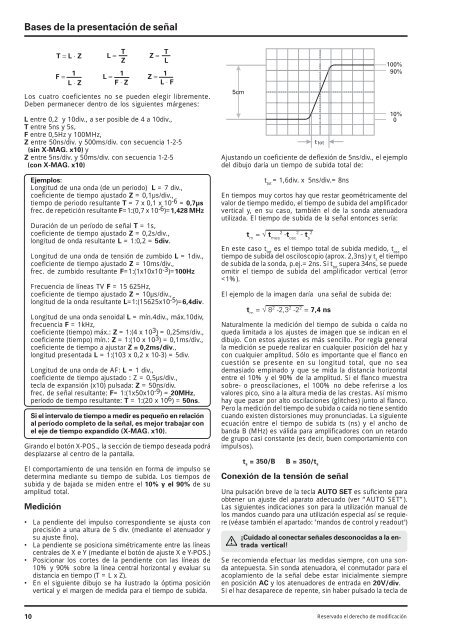• En el siguiente dibujo se ha ilustrado la óptima posición vertical y el margen de medida para el tiempo de subida. . . . . . . . . . . . . . . . . . . . . . . . . . . . . . . . . . . . . . . . . Ajustando un coeficiente de deflexión de 5ns/div., el ejemplo del dibujo daría un tiempo de subida total de: t tot = 1,6div. x 5ns/div.= 8ns En tiempos muy cortos hay que restar geométricamente del valor de tiempo medido, el tiempo de subida del amplificador vertical y, en su caso, también el de la sonda atenuadora utilizada. El tiempo de subida de la señal entonces sería: En este caso t tot es el tiempo total de subida medido, t osc el tiempo de subida del osciloscopio (aprox. 2,3ns) y t s el tiempo de subida de la sonda, p.ej.= 2ns. Si t tot supera 34ns, se puede omitir el tiempo de subida del amplificador vertical (error
Page 1 and 2: El Manual de la Instrucción El Mod
Page 3 and 4: KONFORMITÄTSERKLÄRUNG DECLARATION
Page 5 and 6: Generalidades Instrucciones de mane
Page 7: Bases de la presentación de señal
Page 11 and 12: Mandos de control y readout tecla A
Page 13 and 14: Mandos de control y readout resulta
Page 15 and 16: Mandos de control y readout present
Page 17 and 18: Mandos de control y readout (16) NM
Page 19 and 20: Mandos de control y readout breve p
Page 21 and 22: Mandos de Control y Readout hacia l
Page 23 and 24: Mandos de Control y Readout (33) AC
Page 25 and 26: Mandos de Control y Readout (MAIN M
Page 27 and 28: Menú Puesta en marcha y ajustes pr
Page 29 and 30: Modo de funcionamiento de los ampli
Page 31 and 32: Disparo y deflexión de tiempo t =
Page 33 and 34: Disparo y deflexión de tiempo TV-L
Page 35 and 36: SAVE/RECALL siempre se visualizan l
Page 37 and 38: Funcionamiento en memoria digital p
Page 39 and 40: Plan de chequeo 2. La frecuencia de
Page 41 and 42: Plan de chequeo retícula. ¡No sin
Page 43 and 44: Interfaz RS232 - Control a distanci
Page 45 and 46: 46 Reservado el derecho de modifica

El Manual de la Instrucción El Modelo: 5105A - BK Precision

You also want an ePaper? Increase the reach of your titles

Delete template?

Save as template?