ϵ2 - Le Cermics - ENPC

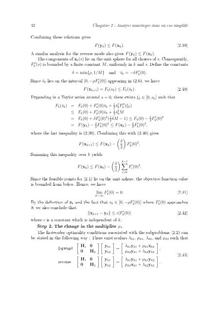
32 Chapitre 2 : Analyse numérique dans un cas simplié
Combining these relations gives
F (y k ) ≤ F (x k ). (2.39)
A similar analysis for the reverse mode also gives F (y k ) ≤ F (x k ).
The components of z k (s) lie on the unit sphere for all choices of s. Consequently,
F ′′
k
(s) is bounded by a nite constant M, uniformly in k and s. Dene the constants
δ = min{ρ, 1/M}
and ¯s k = −δF ′ k(0).
Since ¯s k lies on the interval [0, −ρF k ′ (0)] appearing in (2.6), we have
F (x k+1 ) = F k (s k ) ≤ F k (¯s k ). (2.40)
Expanding in a Taylor series around s = 0, there exists ξ k ∈ [0, s k ] such that
F k (¯s k ) = F k (0) + F k(0)¯s ′ k + 1 2 ¯s2 kF k ′′ (ξ k )
≤ F k (0) + F k(0)¯s ′ k + 1 2 ¯s2 kM
= F k (0) + δF ′ k(0) 2 ( 1 2 δM − 1) ≤ F k(0) − δ 2 F ′ k(0) 2
= F (y k ) − δ 2 F ′ k(0) 2 ≤ F (x k ) − δ 2 F ′ k(0) 2 ,
where the last inequality is (2.39). Combining this with (2.40) gives
F (x k+1 ) ≤ F (x k ) −
Summing this inequality over k yields
F (x k ) ≤ F (x 0 ) −
( δ
2)
F ′ k(0) 2 .
( δ ∑k−1
F i
2) ′ (0) 2 .
i=0
Since the feasible points for (2.1) lie on the unit sphere, the objective function value
is bounded from below. Hence, we have
lim F k(0) ′ = 0. (2.41)
k→∞
By the denition of z k and the fact that s k ∈ [0, −ρF k ′(0)] where F k ′ (0) approaches
0, we also conclude that
‖x k+1 − y k ‖ ≤ c|F k(0)| ′ (2.42)
where c is a constant which is independent of k.
Step 2. The change in the multiplier µ.
The rst-order optimality conditions associated with the subproblems (2.2) can
be stated in the following way : There exist scalars λ k1 , µ k1 , λ k2 , and µ k2 such that
forward [ H 1 0
reverse
] [ ] [ ]
yk1 λk1 y
= k1 + µ k1 x k2
,
0 H 2 y k2 µ k2 y k1 + λ k2 y k2
[ ] [ ]
H1 0 yk1
=
0 H 2 y k2
[ ]
λk1 y k1 + µ k1 y k2
.
µ k2 x k1 + λ k2 y k2
(2.43)