Parte I: Il metodo Strut-and-Tie - Dipartimento di Ingegneria Civile e ...
Parte I: Il metodo Strut-and-Tie - Dipartimento di Ingegneria Civile e ...
Parte I: Il metodo Strut-and-Tie - Dipartimento di Ingegneria Civile e ...

You also want an ePaper? Increase the reach of your titles
YUMPU automatically turns print PDFs into web optimized ePapers that Google loves.
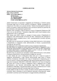
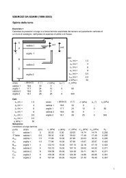
Corso <strong>di</strong> Progetto <strong>di</strong> <strong>Strut</strong>ture II<br />
Meccanismi Puntone-Tirante<br />
Puntone Tirante<br />
per <strong>Strut</strong>ture in Calcestruzzo Armato<br />
<strong>Dipartimento</strong> <strong>di</strong> <strong>Ingegneria</strong> <strong>Civile</strong> e Ambientale<br />
Università <strong>di</strong> Firenze<br />
<strong>Parte</strong> I: <strong>Il</strong> <strong>metodo</strong> <strong>Strut</strong>‐<strong>and</strong>‐<strong>Tie</strong><br />
1/65<br />
2/65<br />
05/05/2010<br />
1
Metodo “puntone‐tirante” (o “<strong>Strut</strong> & <strong>Tie</strong>”)<br />
Origini del <strong>metodo</strong>: W. Ritter (1899), E. Mörsch (1912)<br />
Sviluppi recenti: J. Schlaich, Università <strong>di</strong> Stoccarda<br />
Convegno IABSE Structural Concrete (1991)<br />
Obbiettivo: Progetto delle “zone <strong>di</strong> <strong>di</strong>scontinuità” delle strutture<br />
in calcestruzzo armato.<br />
Strumento: In<strong>di</strong>viduazione <strong>di</strong> un modello puntoni‐tiranti (“<strong>Strut</strong><br />
& <strong>Tie</strong> Model” o “S&T Model”) con puntoni in<br />
calcestruzzo e tiranti in acciaio.<br />
Sella Gerber<br />
Esempi <strong>di</strong> modelli tirante‐puntone<br />
Forze trasversali in unioni che<br />
trasmettono forze <strong>di</strong> compressione<br />
Modello S&T<br />
mensole<br />
3/65<br />
Angoli <strong>di</strong> portali soggetti a<br />
momento flettente negativo<br />
Dettagli costruttivi<br />
mensole tozze<br />
4/65<br />
05/05/2010<br />
2
Zone <strong>di</strong> continuità e <strong>di</strong>scontinuità<br />
In<strong>di</strong>viduazione delle regioni <strong>di</strong> continuità (“B”) e <strong>di</strong> <strong>di</strong>scontinuità (“D”)<br />
Le regioni “D” si estendono<br />
fino ad una <strong>di</strong>stanza h dalla<br />
<strong>di</strong>scontinuità (h = altezza<br />
della sezione<br />
dell’elemento)<br />
D<br />
h<br />
h<br />
D h<br />
l < h<br />
D D<br />
h<br />
h h<br />
B<br />
l > 2 h<br />
D<br />
h 2 h<br />
h<br />
B B<br />
l > 4 h<br />
Esempio <strong>di</strong> identificazione della geometria<br />
D h<br />
1° Passo: in<strong>di</strong>viduazione delle regioni <strong>di</strong> continuità (“B”) e <strong>di</strong> <strong>di</strong>scontinuità (“D”)<br />
B<br />
D<br />
D<br />
D<br />
D<br />
B D B D B D<br />
B<br />
D<br />
D<br />
D<br />
5/65<br />
6/65<br />
05/05/2010<br />
3
2° Passo: identificazione del modello tirante‐puntone all’interno <strong>di</strong> ogni regione “D”, dopo<br />
aver determinato le forze agenti sul suo contorno<br />
B<br />
D<br />
D<br />
D<br />
D<br />
B D B D B D<br />
B<br />
D<br />
D<br />
D<br />
Una volta identificata la geometria, si passa al calcolo degli sforzi normali in tutte le aste<br />
(puntoni e tiranti) del traliccio S&T.<br />
7/65<br />
<strong>Il</strong> comportamento a rottura del cemento armato<br />
<strong>Il</strong> <strong>metodo</strong> S&T dovrebbe in sostanza in<strong>di</strong>viduare il comportamento<br />
a rottura della struttura, allorqu<strong>and</strong>o, formatesi importanti fessure,<br />
si in<strong>di</strong>viduano puntoni <strong>di</strong> calcestruzzo e tiranti <strong>di</strong> armatura armatura.<br />
8/65<br />
05/05/2010<br />
4
Simulazione del comportamento a rottura<br />
Esistono co<strong>di</strong>ci <strong>di</strong><br />
calcolo sofisticati<br />
(ANSYS, DIANA,<br />
ecc.) che sono in<br />
grado <strong>di</strong> prevedere<br />
il comportamento a<br />
rottura <strong>di</strong> strutture<br />
in CA.<br />
Quadro fessurativo sperimentale e simulato<br />
Sperimentale Simulato<br />
9/65<br />
10/65<br />
05/05/2010<br />
5
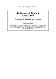
Esempi <strong>di</strong> armatura <strong>di</strong> una mensola tozza<br />
<strong>Il</strong> funzionamento è però non univoco ma <strong>di</strong>pende dalla <strong>di</strong>posizione<br />
dell’armatura tesa.<br />
a) b)<br />
Qual è la scelta progettuale più corretta, il progetto “migliore”?<br />
Criteri <strong>di</strong> progetto<br />
Un criterio <strong>di</strong> progetto può essere quello <strong>di</strong> scegliere fra tutti i<br />
tralicci possibili quello che, a parità <strong>di</strong> acciaio, ha la rigidezza<br />
maggiore.<br />
P �u<br />
� �<br />
N<br />
2<br />
i l i<br />
i E i Ai<br />
11/65<br />
(1)<br />
Esempio <strong>di</strong> ricerca della<br />
massima rigidezza attraverso<br />
un processo <strong>di</strong> ottimizzazione<br />
<strong>Il</strong> concetto può essere chiarito con un esempio: dato un traliccio <strong>di</strong> N aste,<br />
determinare la struttura <strong>di</strong> massima rigidezza tra tutte quelle possibili che si<br />
ottengono elimin<strong>and</strong>o M aste (M
1) Metodo del percorso <strong>di</strong> carico (J. Schlaich)<br />
(“load path method”)<br />
Si in<strong>di</strong>viduano in fase elastica i flussi <strong>di</strong> tensione e si sostituiscono con le forze<br />
risultanti.<br />
Puntone in c.a. compresso<br />
Tirante in acciaio <strong>di</strong> armatura teso<br />
13/65<br />
2) Metodo delle linee <strong>di</strong> <strong>di</strong>spluvio (Università <strong>di</strong> Firenze)<br />
Si rappresenta in 3D lo stato tensionale in<strong>di</strong>vidu<strong>and</strong>o le linee <strong>di</strong> massimi locali<br />
delle tensioni principali (linee <strong>di</strong> <strong>di</strong>spluvio)<br />
14/65<br />
05/05/2010<br />
7
3) Metodo dell’abbattimento del modulo elastico<br />
(Università <strong>di</strong> Firenze)<br />
In un processo iterativo, si effettuano analisi agli elementi finiti in campo elastico<br />
lineare e si “sottraggono” progressivamente gli elementi meno sollecitati<br />
(abbattendo il modulo elastico) .<br />
4) Metodo <strong>di</strong> ottimizzazione topologica<br />
15/65<br />
Consiste nel ricercare la massima rigidezza utilizz<strong>and</strong>o solo una frazione <strong>di</strong> del<br />
volume <strong>di</strong> materiale. In pratica si ricerca una <strong>di</strong>stribuzione <strong>di</strong> densità <strong>di</strong> materiale<br />
tale da minimizzare l’energia <strong>di</strong> deformazione fissati alcuni vincoli.<br />
16/65<br />
05/05/2010<br />
8
a b<br />
Modello MTOTP del setto Andamento dei flussi <strong>di</strong> compressione<br />
<strong>Parte</strong> II: Normativa<br />
17/65<br />
18/65<br />
05/05/2010<br />
9
Verifiche secondo N.T.C. 2008<br />
Bozza della Circolare relativa alle N.T.C. 2008<br />
(esempio <strong>di</strong> verifica <strong>di</strong> mensola tozza)<br />
Si possono utilizzare due meccanismi resistenti in parallelo fra loro<br />
1) Con armatura superiore 2) Con armatura inclinata<br />
19/65<br />
Ve<strong>di</strong> EC<br />
20/65<br />
05/05/2010<br />
10
Meccanismo con tirante orizzontale<br />
0.4 b d f cd c sin 2 ψ<br />
del tirante in acciaio per sod<strong>di</strong>sfare la gerarchia delle resistenze.<br />
21/65<br />
Equivale a verificare un puntone <strong>di</strong> calcestruzzo <strong>di</strong> altezza<br />
0.4 c d sinψ, nel caso <strong>di</strong> puntone inclinato a 45° l’altezza<br />
varia da 0.28 d a 0.42 d, in funzione del valore <strong>di</strong> c (1 o 1.5).<br />
22/65<br />
05/05/2010<br />
11
Meccanismo con tirante inclinato<br />
P c<br />
Equivale a verificare un puntone <strong>di</strong><br />
calcestruzzo <strong>di</strong> altezza 0.2 d.<br />
Ve<strong>di</strong> EC2, appen<strong>di</strong>ce J<br />
23/65<br />
24/65<br />
05/05/2010<br />
12
Esempio<br />
Verifiche secondo EC2<br />
1. Verifiche dei puntoni<br />
2. Verifiche dei tiranti<br />
3. Verifiche dei no<strong>di</strong><br />
25/65<br />
26/65<br />
05/05/2010<br />
13
Verifica dei puntoni compressi<br />
in assenza <strong>di</strong> azioni trasversali <strong>di</strong> trazione<br />
in presenza <strong>di</strong> azioni trasversali <strong>di</strong> trazione<br />
Le armature metalliche sono utilizzate come:<br />
1. tiranti del modello tirante‐puntone<br />
Verifica dei tiranti<br />
2. elementi resistenti alle forze <strong>di</strong> trazione<br />
ortogonali ai puntoni<br />
C<br />
C<br />
27/65<br />
28/65<br />
05/05/2010<br />
14
Tiranti che assorbono gli sforzi <strong>di</strong> trazione<br />
ortogonali ai puntoni<br />
In funzione del rapporto <strong>di</strong> snellezza H/b (H e b sono rispettivamente l’altezza e la larghezza<br />
del puntone) in un puntone possono aversi sia regioni tipo “B” sia regioni tipo “D” o soltanto<br />
queste q ultime.<br />
b<br />
F<br />
F<br />
Equilibrio alla<br />
rotazione attorno a<br />
H ��� b<br />
b<br />
b<br />
a<br />
F<br />
D<br />
B<br />
D<br />
Discontinuità parziale<br />
F<br />
b<br />
a/4<br />
H ���<br />
b<br />
a<br />
b<br />
Discontinuità totale<br />
b<br />
a/4 a/4<br />
F/2 F/2<br />
a<br />
F<br />
Puntone con <strong>di</strong>scontinuità parziale<br />
b<br />
b<br />
T<br />
2<br />
b<br />
�<br />
b/2<br />
F/2<br />
b/4<br />
b<br />
F � b a �<br />
� � �<br />
2 � 4 4 �<br />
F/2<br />
b/4<br />
F<br />
b<br />
F/A<br />
b<br />
b/2<br />
b/4<br />
F/2<br />
F/2<br />
F � a �<br />
T � �1� �<br />
4 � b�<br />
�<br />
a/4<br />
T<br />
C=T<br />
29/65<br />
30/65<br />
05/05/2010<br />
15
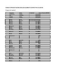
Andamento della forza trasversale e dell’inclinazione � dei<br />
puntoni inclinati al variare <strong>di</strong> a/b.<br />
T/F / �<br />
0,4 90°<br />
b<br />
0,3<br />
0,2<br />
01 0,1<br />
Equilibrio<br />
80°<br />
70°<br />
60°<br />
b<br />
F<br />
F<br />
h= =H/2<br />
Ipotesi sulla <strong>di</strong>ffusione<br />
delle tensioni<br />
approx<br />
T = 0,25 F (1 − a/b)<br />
T/F<br />
teoria elastica lin.<br />
0,1 0,3 0,5 0,7 0,9 a/b<br />
Puntone con <strong>di</strong>scontinuità totale<br />
h=H/22<br />
h/2 h a/4<br />
Tz<br />
b ef<br />
F/2<br />
bef/4<br />
a<br />
a/4 a/4<br />
F/2 F/2<br />
bef<br />
b<br />
ef � �<br />
F/2<br />
F �ba� � �<br />
2 � 4 4�<br />
bef/4<br />
� 0,5 H � 0,65 a<br />
z � h/2 �<br />
H/4<br />
�<br />
h=H/22<br />
h/2 h a/4<br />
F/2<br />
F/2<br />
a/4<br />
bef/4<br />
31/65<br />
C=T<br />
T<br />
F � a �<br />
T � �1�0,7 �<br />
4 � H�<br />
32/65<br />
05/05/2010<br />
16
Esempio<br />
σ � k �'<br />
f<br />
1Rd, max<br />
(k 1 =1,0)<br />
σ � k �'<br />
f<br />
2Rd, max<br />
Nodo compresso senza tiranti<br />
2<br />
1<br />
cd<br />
cd<br />
33/65<br />
Nodo compresso‐teso con armatura <strong>di</strong>sposta in una <strong>di</strong>rezione<br />
Esempio<br />
(k 2 =0,85)<br />
34/65<br />
05/05/2010<br />
17
Nodo compresso‐teso con armatura <strong>di</strong>sposta in due <strong>di</strong>rezioni<br />
Esempio<br />
σ � k �'<br />
f<br />
3Rd, max<br />
3<br />
(k 3 =0,75)<br />
cd<br />
Mensola tozza<br />
a c < h c/2 a c > h c/2<br />
Armatura<br />
secondaria<br />
orizzontale<br />
a c<br />
F F<br />
Ed<br />
Ed<br />
h c<br />
a c<br />
Armatura<br />
secondaria<br />
verticale<br />
h c<br />
35/65<br />
36/65<br />
05/05/2010<br />
18
400<br />
400<br />
150<br />
125<br />
250<br />
50 150<br />
400 250<br />
Armatura principale<br />
F Ed<br />
Mensola tozza con a c
F t<br />
F c<br />
Armatura principale<br />
come esempio precedente<br />
Mensola tozza con a c>h c/2<br />
a<br />
a ac a /2 a /2<br />
F<br />
Ed<br />
z<br />
h c<br />
traliccio iperstatico<br />
Armatura secondaria<br />
ipotesi <strong>di</strong> variazione lineare <strong>di</strong> Fwd nel tirante<br />
verticale al variare <strong>di</strong> a tra il valore Fwd =0pera=<br />
z/2 e F F per a 2 z<br />
F<br />
wd<br />
2 FEd<br />
F<br />
� a �<br />
3 z 3<br />
2a/z �1<br />
� FEd<br />
3<br />
z/2 e F wd = F Ed per a = 2�z 3<br />
F’t<br />
a a<br />
F’<br />
Ed<br />
F’’<br />
Ed<br />
z z<br />
F’c<br />
TRALICCIO 1<br />
F’’t<br />
F’’c<br />
a/2 a/2<br />
Ed<br />
39/65<br />
�<br />
TRALICCIO 2<br />
40/65<br />
05/05/2010<br />
20
Pressioni localizzate (EC2 §6.7)<br />
41/65<br />
42/65<br />
05/05/2010<br />
21
43/65<br />
44/65<br />
05/05/2010<br />
22
<strong>Parte</strong> III: Altri esempi<br />
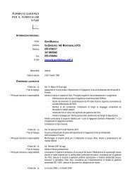
Esempio: Sella Gerber<br />
45/65<br />
L’EC2 consiglia <strong>di</strong> utilizzare uno dei due tralicci in figura:<br />
schema b) bordo inferiore completamente privo <strong>di</strong> armature<br />
schema a) occorre un’armatura longitu<strong>di</strong>nale superiore per ancoraggio staffe ed<br />
armatura <strong>di</strong> confinamento del puntone inclinato C1<br />
675<br />
C1<br />
1<br />
500<br />
425<br />
�<br />
3<br />
T1<br />
725<br />
�<br />
45°<br />
C2<br />
C3<br />
2<br />
725 580<br />
T2<br />
700<br />
C1<br />
1<br />
4 3<br />
2<br />
500<br />
T1<br />
2025<br />
a) b)<br />
Materiali:<br />
calcestruzzo C35/45 f ck = 35 N/mm 2<br />
acciaio B450C f yk = 450 N/mm 2<br />
45°<br />
1305<br />
C2<br />
45°<br />
C3<br />
T2<br />
4<br />
46/65<br />
05/05/2010<br />
23
Traliccio a) R=R Sdu /2 = 500 kN<br />
il corrente compresso ha una larghezza pari alla profon<strong>di</strong>tà x dell’asse neutro della sezione e<br />
pertanto <strong>di</strong>sta x/2 dal lembo superiore; dall’equilibrio alla traslazione della sezione si ottiene<br />
x=99 mm<br />
C 1<br />
�<br />
R<br />
senα<br />
T2 1<br />
� 620 kN<br />
� C � cosα � 366 kN<br />
T2<br />
C 2 �<br />
� 260 kN<br />
senβ � cosβ<br />
senβ<br />
� � C � 230 kN<br />
sen45� 45�<br />
C3 2<br />
T1 1<br />
2<br />
� C �senα<br />
� C �senβ<br />
� 663 kN<br />
Traliccio b) R=R Sdu /2 = 500 kN<br />
C'1 � 500 kN<br />
� C' � 500 kN<br />
C'2 1<br />
366000<br />
A s1 � � 935 mm<br />
391,3<br />
663000<br />
A s1 � � 1694 mm<br />
391,3<br />
T' T'1 � 2 � C' C'1<br />
� 707 kN sii adottano d tt llestesse t armature t <strong>di</strong> T’ 2<br />
C'3 1<br />
� T' � 707 kN<br />
�T' �C'<br />
��cos45� � 1000 kN<br />
T'2 � 1 3<br />
700<br />
1000000<br />
A �<br />
391,3<br />
2<br />
2<br />
675<br />
C1<br />
1<br />
500<br />
425<br />
�<br />
4<br />
3<br />
T1<br />
725<br />
�<br />
45°<br />
C2<br />
C3<br />
2<br />
725 580<br />
T2<br />
47/65<br />
2<br />
s1 � 2556 mm si adottano 6�24 = 2712 mm2 2 4<br />
1<br />
500<br />
C1’<br />
T1’<br />
2025<br />
45°<br />
1305<br />
C2’<br />
3<br />
45°<br />
C3’<br />
T2’<br />
48/65<br />
05/05/2010<br />
24
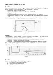
3500<br />
750<br />
Trave ad altezza variabile<br />
3000 3000<br />
2000<br />
F F<br />
A A<br />
1500<br />
6250 8500<br />
22500<br />
F = 1200 kN<br />
(si trascura il peso proprio della trave)<br />
6250 750<br />
Materiali: calcestruzzo C30/37 f ck = 30 N/mm 2 , acciaio B450C f yk = 450 N/mm 2<br />
Regioni B e D<br />
0,85f<br />
1,5<br />
0,85 � 30<br />
1,5<br />
ck<br />
f cd � � �<br />
17<br />
N/mm<br />
f yk 450<br />
f yd � � � 391,3 N/mm<br />
1,15 1,15<br />
D 1<br />
ck yk<br />
F F<br />
D 2<br />
D 3<br />
B<br />
A A<br />
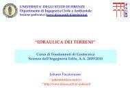
Caratteristiche <strong>di</strong> sollecitazione<br />
1200 kN<br />
A<br />
3000<br />
F<br />
Taglio<br />
2<br />
Momento flettente<br />
2<br />
F<br />
D 2<br />
15000 3000<br />
A<br />
3600 kNm<br />
D 1<br />
300<br />
49/65<br />
50/65<br />
05/05/2010<br />
25
35000<br />
Forze risultanti sulla regione D<br />
30001200 kN<br />
3500<br />
1690 210<br />
750<br />
Percorso <strong>di</strong> carico<br />
3500<br />
750<br />
1200 kN<br />
6250 2000<br />
2130 kN<br />
2130 kN<br />
3000 1200 kN 210<br />
3000<br />
1200 kN<br />
Modello puntoni‐tiranti<br />
A<br />
6250 2000<br />
F loop<br />
2130 kN<br />
2130 kN<br />
1200 kN 1200 kN<br />
C 2<br />
B<br />
C3 E<br />
C4 D<br />
T 2<br />
C1 T 1<br />
T 3<br />
C5 C<br />
45°<br />
1200 kN 1500<br />
750<br />
1200 kN<br />
1500<br />
210<br />
1690<br />
100<br />
1690<br />
100<br />
100<br />
C 4<br />
C 5<br />
51/65<br />
C1 ve<strong>di</strong> calcolo forze nella regione B 2130 kN<br />
T1 C 2<br />
T3 T2 C3 Floop C4 C5 T1=C1 (equil. (q verticale nodo A) )<br />
(equil. orizzontale nodo A)<br />
T2 = T3, perché C5 è inclinato <strong>di</strong> 45° (equil. nodo C)<br />
(equil. orizzontale nodo B)<br />
Floop = C1 –C3 (equil. verticale nodo C)<br />
2130 kN<br />
1647 kN<br />
1128 kN<br />
1128 kN<br />
1128 kN<br />
1002 kN<br />
1509 kN<br />
1595 kN<br />
52/65<br />
210<br />
31990<br />
100<br />
05/05/2010<br />
26
53/65<br />
54/65<br />
05/05/2010<br />
27
55/65<br />
56/65<br />
05/05/2010<br />
28
<strong>Parte</strong> IV: Analisi <strong>di</strong> parete forata<br />
57/65<br />
58/65<br />
05/05/2010<br />
29
Esempio <strong>di</strong> armatura <strong>di</strong> una trave forata<br />
Traliccio isostatico Traliccio iperstatico<br />
Quattro <strong>di</strong>fferenti esempi <strong>di</strong> armatura<br />
1) Traliccio isostatico<br />
2) Traliccio iperstatico<br />
3) Traliccio isostatico con la stessa quantità <strong>di</strong> armatura del traliccio iperstatico<br />
4) Armatura progettata come se si trattasse <strong>di</strong> una trave snella<br />
59/65<br />
Tirante 1. Modello STM iperstatico 2. Modello STM isostatico<br />
Fo<br />
rza (kN)<br />
T1 10<br />
70<br />
T2 53<br />
5<br />
T3 10<br />
70<br />
T4 53<br />
5<br />
T5 10<br />
70<br />
T6 53<br />
5<br />
T7 53<br />
5<br />
T8 53<br />
5<br />
T9 66<br />
3<br />
Peso armatura (kg)<br />
Armatura<br />
6 Ø 18 + 4 Ø 24<br />
6 Ø 18<br />
2 x 5 Ø 18<br />
2 x 5 Ø 18<br />
2 x 5 Ø 18<br />
2 x 5 Ø 12<br />
2 x 5 Ø 18<br />
2 x 5 Ø 12<br />
2 Ø 24 + 2 Ø 24<br />
Dettagli delle armature<br />
Lunghezza g<br />
(cm)<br />
250<br />
450<br />
460<br />
460<br />
460<br />
260<br />
460<br />
260<br />
540<br />
For<br />
za (kN)<br />
107<br />
0<br />
/<br />
/<br />
/<br />
/<br />
/<br />
/<br />
/<br />
132<br />
6<br />
Armatura<br />
6 Ø 18 + 4 Ø<br />
24<br />
Lunghezza g<br />
(cm)<br />
250<br />
/ /<br />
/ /<br />
/ /<br />
/ /<br />
/ /<br />
/ /<br />
/ /<br />
4 Ø 24 + 4 Ø<br />
24<br />
540<br />
3. Modello STM isostatico con<br />
armatura equivalente<br />
Armatura<br />
Lunghezza g<br />
(cm)<br />
8 Ø 24 + 2 Ø<br />
20 250<br />
6 Ø 18<br />
/<br />
/<br />
/<br />
/<br />
/<br />
/<br />
12 Ø 24 + 2 Ø<br />
20<br />
450<br />
/<br />
/<br />
/<br />
/<br />
/<br />
/<br />
4. Dimension. errato<br />
Armatura Lunghezza<br />
(cm)<br />
10 Ø 20<br />
10 Ø 20<br />
250<br />
450<br />
/ /<br />
/ /<br />
/ /<br />
/ /<br />
423 271 421 171<br />
540<br />
/<br />
/<br />
/<br />
/<br />
/<br />
/<br />
60/65<br />
05/05/2010<br />
30
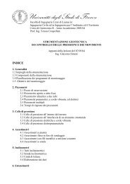
Esempio <strong>di</strong> armatura <strong>di</strong> una trave forata<br />
Curve carico‐spostamento<br />
Carico (KN)<br />
7.E+03<br />
6.E+03<br />
5.E+03<br />
4.E+03<br />
3.E+03<br />
2.E+03<br />
1.E+03<br />
0.E+00<br />
Traliccio Iperstatico<br />
Traliccio isostatico<br />
Progetto errato<br />
Traliccio isostatico con<br />
armatura equivalente<br />
0 0.1 0.2 0.3 0.4 0.5<br />
Spostamento verticale (cm)<br />
Esempio <strong>di</strong> simulazione<br />
Calcestruzzo Acciaio Armature<br />
Ec = 31200 N/mm2 Es = 210000 N/mm2 T1: 6Ø18 + 4Ø24<br />
ν = 0.2 ν = 0.2 T9: 8Ø24<br />
ft = 2.6 N/mm2 Gf = 100J/m<br />
<strong>di</strong>ffusa: 2x Ø8 20”<br />
2<br />
61/65<br />
Modellazione: 496 elementi soli<strong>di</strong> (SDM)<br />
6 elementi soli<strong>di</strong> elastici lineari (supporti in acciaio)<br />
2270 elementi biella elastici lineari (armature <strong>di</strong>screte)<br />
62/65<br />
05/05/2010<br />
31
63/65<br />
Puntoni<br />
e<br />
Tiranti<br />
64/65<br />
05/05/2010<br />
32
Distribuzione delle tensioni <strong>di</strong> armatura e quadro fessurativo nel caso <strong>di</strong><br />
traliccio isostatico (configurazione a rottura)<br />
65/65<br />
05/05/2010<br />
33