LISREL / SIMPLIS: Strategien zur Beurteilung der Modellanpassung ...

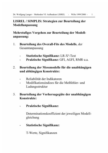
Dr. Wolfgang Langer - Methoden VI: Aufbaukurs LISREL - WiSe 1999/2000 - 1
LISREL / SIMPLIS: Strategien zur Beurteilung der
Modellanpassung
Mehrstufiges Vorgehen zur Beurteilung der Modellanpassung:
1. Beurteilung des Overall-Fits des Modells, der
Gesamtanpassung
- Statistische Signifikanz: LR-X²-Test
- Praktische Signifikanz: GFI, AGFI, RMR u.a.
2. Beurteilung der Messmodelle für die unabhängigen
und abhängigen Konstrukte:
- Reliabilität der Indikatoren
- Modifikationsindizes für die Meßfehler- und
Ladungsstruktur
3. Beurteilung der Vorhersagegüte der unabhängigen
Konstrukte:
- Praktische Signifikanz:
Determinationskoeffizient der jeweiligen Modellgleichung
- Statistische Signifikanz:
T-Werte, Signifikanzen

Dr. Wolfgang Langer - Methoden VI: Aufbaukurs LISREL - WiSe 1999/2000 - 2
Alle drei Prüfungsschritte sind durchzuführen, da eine alleinige Favorisierung der Überprüfung
der Gesamtmodellanpassung zu einer vorschnellen Falsifikation von Kausalmodellen führen
kann, wie Sobel & Bohrnstedt (1984, S. 158) bereits bemerkt haben:
"Scientific progress could be impeded if fit coefficients ... are used as the primary criterion for
judging the adequacy of a model."
Wheaton (1988, S. 199) schlägt daher vor, erstens die drei obigen Prüfungsschritte einzuhalten
und zweitens mehrere Maßzahlen zur Beurteilung der Modellanpassung zu verwenden.
1. Schritt: Beurteilung der Gesamtanpassung
a) Statistische Signifikanz:
Likelihood-Ratio-X²-Test: (Zentrale-X²-Verteilung)
1. Fall: Annahme: Das spezifizierte Modell gilt exakt für die Grundgesamtheit !
LR $² (n 1) F[S,(ˆ)]
F: Minimum der Schätzfunktion
S: Beobachtete Korrelations /Kovarianzmatrix
: Unter Restriktionen geschätzte Korrelations
/Kovarianzmatrix
Mit folgender Anzahl von Freiheitsgraden:
D.F. s t
Anzahl der nichtredundanten Elemente der Stichprobenmatrix S:
k(k 1)
s
2
t: Anzahl der unabhängig geschätzten Parameter
k: Anzahl der Indikatoren
Die Nullhypothese H 0 des LR-X²-Anpassungstests lautet: ("Badness of fit test")
Die Abweichungen der Elemente der beobachteten und unter Restriktionen geschätzten
Korrelations-/Kovarianzmatrix weichen statistisch nicht bedeutsam voneinander ab.
D.h., das spezifizierte Strukturmodell reproduziert die beobachtete Eingabematrix
nahezu vollständig.

Dr. Wolfgang Langer - Methoden VI: Aufbaukurs LISREL - WiSe 1999/2000 - 3
Die Alternativehypothese H A lautet:
Die modellimmanent geschätzte Korrelations-/Kovarianzmatrix weicht statistisch
bedeutsam von der beobachteten Stichprobenmatrix ab.
Ziel der Analyse ist es, ein Modell zu finden, dessen Residuen nicht statistisch signifikant
ausfallen. Da dieser Test sehr empfindlich auf den Stichprobenumfang reagiert -
hohe Fallzahlen führen zu Falsifikation fast jeder Modellstruktur (n 200), Modelle mit
geringen Fallzahlen können faktisch nicht widerlegt werden (n 100) - entwickelten
Jöreskog&Sörbom (1989) zwei Maßzahlen der praktischen Signifikanz zur Beurteilung
des Modellfits, die beide der allgemeinen Logik der Proportionalen Fehlerreduktion
folgen, wie sie auch dem Determinationskoeffizienten R 2 zugrunde liegt.
2. Fall: Modell gilt nur annäherungsweise für die Grundgesamtheit
Für diesen Fall empfiehlt Browne (1984) die Verwendung der nichtzentralen X²-Verteilung
mit dem Nichtzentralitätsparameter (lambda) und d-Freiheitsgraden. Dieser
Lageparameter läßt sich anhand der Stichprobenverteilung folgendermaßen schätzen: 1
Schätzung des Nichtzentralitätsparameters:
ˆ Max[(Likelihood Ration $ 2 WLS D.F.),0]
Mit Hilfe des mitgelieferten DOS-Utility-Programms “LISPOWER.EXE” können wir
nun uns den kritischen Wert der nichtzentralen X²-Verteilung bei einer bestimmten
Anzahl von Freiheitsgraden d, einem geschätzten Nichtzentralitätsparameter sowie
einem vorgegebenen .-Niveau (Irrtumswahrscheinlichkeit) ermitteln lassen.
Ab der Version 8.30 berechnet LISREL automatisch neben dem Nichtzentralitätsparameter
den zugehörigen nichtzentralen X²-Anpassungstest für die mit Hilfe der WLS-
Schätzung reproduzierte Korrelations-/ Kovarianzmatrix.
1 S. Jöreskog & Sörbom 1993, S.117

Dr. Wolfgang Langer - Methoden VI: Aufbaukurs LISREL - WiSe 1999/2000 - 4
b) Praktische Signifikanz: Klassische Maße für LISREL !
Globale Anpassungsmaße:
- Goodness of Fit-Index (GFI)
- Adjusted Goodness of Fit Index (AGFI)
- Root Mean squared Residuals (RMR)
Die beiden ersten Indizes beruhen auf einer Normierung des LR-$²-Werts, wobei der
AGFI zusätzlich die Anzahl der Indikatoren und Freiheitsgrade berücksichtigt. Beim
RMR handelt es sich um die Größe des geschätzten durchschnittlichen Residuums des
Strukturgleichungsmodells. Je größer das durchschnittliche Residuum ausfällt, desto
schlechter ist die Modellanpassung.
Goodness of Fit Index (GFI) 1
[0;1]
F[S,( ˆ)
F[S,(0)]
Inhaltlich: Prozentsatz der Informationen von S,
der durch das Kausalmodell reproduziert wird.
S: Beobachtete Korrelations /Kovarianzmatrix
: Modellimmanent reproduzierte Korrelations /Kovarianzmatrix
Adjusted Goodness of Fit Index (AGFI)
1
( p q )(p q 1)
2D.F.
(1 GFI )
[0;1]
p: Anzahl der Y Indikatoren
q: Anzahl der X Indikatoren
D.F.: Anzahl der Freiheitsgrade

Dr. Wolfgang Langer - Methoden VI: Aufbaukurs LISREL - WiSe 1999/2000 - 5
Root Mean Squared Residual (RMR)
p q
2
i 1
i
j 1
(s ij
1 ij
) 2
(pq) (pq1)
p: Anzahl der Y Indikatoren
q: Anzahl der X Indikatoren
Faulbaum (1981, S. 22-44) schlägt für das GFI, AGFI sowie das RMR-Maß folgende Schwellenwerte
für die Beurteilung der Modellanpassung an die empirische Stichprobe vor:
Tab.1:
LISREL/SIMPLIS: Kriterien für die Beurteilung
der Modellanpassung (Daumenregeln)
Quelle: Faulbaum, F.: Konfirmatorische Analysen der Reliabilität von Wichtigkeitseinstufungen
beruflicher Merkmale. ZUMA-Nachrichten, 9 (1981), S.22-44
Modellfit: GFI: AGFI: RMR:
vollständig bestätigt
0.98 0.95 0.05
tendentiell bestätigt
0.95 GFI < 0.98 0.90 AGFI < 0.95 0.05 RMR < 0.10
insgesamt abgelehnt
< 0.95 < 0.90 > 0.10
Für den Likelihood-Ratio-$²-Test gilt, wenn die Irrtumswahrscheinlichkeit p 0.10 ausfällt,
d.h., niedriger als 10 % ist, gilt die spezifizierte Modellstruktur für die vorliegende
Stichprobe als falsifiziert (widerlegt).

Dr. Wolfgang Langer - Methoden VI: Aufbaukurs LISREL - WiSe 1999/2000 - 6
Andere LR-X²-basierte globale Anpassungsmaße
1. Akaike-Information-Criterium
Akaike Information Criterium:
AIC c D.F.
c: L.R.$ 2 der aktuellen Modells
D.F.: Anzahl unabhängig geschätzten Parameter
Interpretation des AIC-Maßes:
Beim Vorliegen mehrerer alternativer Modelle wähle dasjenige aus, dessen AIC-Wert am
niedrigsten ist.
2. Bozdogans Corrected-Akaike-Information-Criterium
Die von Bozdogan vorgeschlagene Korrektur des Akaike-Information-Kriteriums berücksichtigt
zusätzlich zur Parameteranzahl den Stichprobenumfang. Für das CAIC gilt dieselbe Anwendungsregel
wie für das AIC.
Bozdogans Corrected Information Criterium:
CAIC c (1 ln n)D.F.
n : Stichprobenumfang

Dr. Wolfgang Langer - Methoden VI: Aufbaukurs LISREL - WiSe 1999/2000 - 7
3. Browne & Cudeck: Single-sample-cross-validation index (ECVI)
Browne und Cudeck (1993) haben einen Index vorgeschlagen, der auf der Idee der “Kreuzvalidierung”
anhand gesplitteter Substichproben beruht. Es mißt das Ausmaß der Übereinstimmung
zwischen der modellimmanent geschätzten Kovarianzmatrix der Analysestichprobe und derjenigen,
die beim identischen Stichprobenumfang aus der Validierungsstichprobe reproduziert wird.
Bei der von Jöreskog & Sörbom implementierten Variante handelt es sich lediglich um eine
Transformation des LR-X²-Werts.
Browne&Cudeck Single Sample Cross Validation Index:
ECVI L.R.$2 M A
n
2
D.F. M A
n
4. Hoelter: Critical N (CN)-Maß
Hoeltern schlug eine Umkehrung der Logik des LR-X² Tests in dem Sinne vor, daß er sich
fragte, ab welchem Stichprobenumfang beim vorliegenden Wert des LR-X²-Tests die Nullhypothese
der vollständigen Reproduktion der Stichprobenkovarianzmatrix zurückgewiesen werden
muß. Für die Beurteilung des Modells stellt er folgende „Daumenregeln“ auf:
“Hoelter suggests, with some care, a threshold level of 200 (times the number of groups in a
multisample analysis) for this measure. This means that a model has an acceptable fit should
have a CN of at least 200 (per sample).” (Wheaton 1988, S. 203)
Hoelter Critical N:
CN L.R.$2 1 .
F(S,(ˆ))
Das von Hoelter vorgeschlagene „Criticial-N“-Maß eignet sich m.E. am ehesten dazu, abzuschätzen,
ob bei der bekannten Sensitivität des LR-$ 2 -Test für große Stichprobenumfänge das
betrachtete Strukturmodell überhaupt eine Chance hat, nicht falsifiziert zu werden. Liegt das
Kritische N bei einem vorgegebenen Signifikanzniveau von 5 oder 10 % deutlich niedriger als
der aktuelle Stichprobenumfang, so ist Widerlegung der Nullhypothese unvermeidlich. Daher
eignet sich das von Hoelter vorgeschlagenen Fitmaß eher zu Abschätzung der Stärke des LR-$ 2
-Tests als zur Beurteilung der Modellanpassung. (S. Bollen&Liang 1988)

Dr. Wolfgang Langer - Methoden VI: Aufbaukurs LISREL - WiSe 1999/2000 - 8
Maße der partiellen / relativen Modellanpassung
Alle Maße partiellen Modellanpassung beruhen auf derselben Grundidee. Hierbei vergleichen
sie den Fit / die Anpassung des aktuellen Modells (M A ) mit derjenigen eines zuvor gewählten
und geschätzten Vergleichsmodells. Bei diesem Modell handelt es sich jeweils um ein restriktiver
spezifiziertes Modell (M R ), das über weniger Schätzer verfügt. Als “absoluter Vergleichsmaßstab”
dient ein sogenanntes Nullmodell (M 0 ), das von der statistischen Unabhängigkeit der
beobachteten Indikatoren ausgeht. Dieses “Nullmodell” schätzt lediglich die Varianzen der
beobachteten Indikatoren. Alle Kovarianzen werden auf Null restringiert oder gesetzt.
Die von einer Reihe von Autoren vorgeschlagenen partiellen Anpassungsmaße sind in LISREL
8 .30 implementiert und verfügen über die folgenden gemeinsamen Definitionsbestandteile:
F A
: Minimum der Fit Funktion des aktuellen Modells (M A
)
F 0
: Minimum der Fit Funktion des Nullmodells (M 0
)
d A
: Anzahl der Freiheitsgrade von M A
d 0
: Anzahl der Freiheitsgrade von M 0
f A
nF A
d A
L.R.$ M A
2
d A
f 0
nF 0
d 0
L.R.$ M 0
2
d 0
2 A
Max(nF A
d A
,0):Nichtzentralitätsparamter M A
2 0
Max(nF 0
d 0
,0):Nichtzentralitätsparamter M 0
Eines der ersten Incremental Fit-Maße haben Bentler&Bennett (1980) entwickelt. Ihr Ziel
bestand darin, entsprechend der Logik der Proportionalen Fehlerreduktion ein Fitmaß zu
entwickeln, das auf den Wertebereich von Null bis Eins normiert ist und sich analog zum
Determinationskoeffizienten R 2 interpretieren läßt. Sie schlugen den Normed-Fit-Index sowie
den Non-Normed-Fit-Index vor.

Dr. Wolfgang Langer - Methoden VI: Aufbaukurs LISREL - WiSe 1999/2000 - 9
1. Bentler&Bonetts (1980) Normed Fit Index (NFI):
Bentler&Bonnett Normed FIT Index 1980:
Bollens û 1
Index 1989:
NFI 1 F A
F 0
1 L.R.$2 M A
L.R.$ 2 M 0
[0;1]
2. Bentler&Bonetts (1980) Non Normed Fit Index (NNFI):
Bentler&Bonetts Non Normed Fit Index (NNFI) 1980:
Tucker Lewis Index (TLI) 1973:
Bollen !2 (rho2) 1989:
L.R.$ 2 M 0
L.R.$ 2 M A
NNFI f 0 f A
f 0
1 d M0
d MA
L.R.$ 2 M 0
1
d M0
Für die Interpretation ihrer NFI und NNFI-Indizes geben Bentler&Benett (1980) folgende
„Daumenregel“ an:
„Since the scale of the fit indices is not necessarily easy to interpret (e.g., the indices are not
squared multiple correlations), experience will be required to establish values of the indices
that are associated with various degrees of meaningfulness of results. In our experience, models
with overall fit indices of less than .9 can usually be improved substantially. These indices, and
the general hierarchical comparision described previously, are best understood by examples.“
(Dies. 1980, S. 600)
Mit Hilfe ihrer Simualtionsstudien haben Marsh, Balla&Hau (1996) eine Vielzahl von Fit-
Indizes im Hinblick auf ihr Eignung für die praktische Datenanalyse überprüft. Hierbei haben
sie nachgewiesen, daß die Größe des NFI vom Stichprobenprobenumfang direkt abhängig ist.
Hingegen empfehlen sie als partielles Anpassungmaß den von Tucker&Lewis (1973) entwickel-

Dr. Wolfgang Langer - Methoden VI: Aufbaukurs LISREL - WiSe 1999/2000 - 10
ten Index, welchen Bentler&Bonnett (1980) später als Non-Normed-Fit-Index bezeichneten.
Bollen (1989) führte für ihn in seinem LISREL-Buch die Bezeichnung !2 ein. Ihres Erachtens
verfügt der NNFI oder TLI über folgende Vorteile, die seine besondere Eignung für die Beurteilung
der Modellanpassung rechtfertigen:
1. Er ist unabhängig von der Stichprobengröße.
2. Er berücksichtigt adäquat die Modellkomplexität als Manus.
3. Er erfaßt systematisch Unterschiede der Fehlspezifikation des Modells.
4. Ausreißer mit Indexwerten über 1.0 treten in der praktischen Datenanalyse sehr selten
auf.
Um diese Ausreißer zu eliminieren, empfehlen Marsh, Balla & Hau (1996, S.331) daher die
folgende Normierung für den Tucker-Lewis-Index (TLI):
Normierungsvorschrift für den Tucker Lewis Index (TLI oder NNFI)
zur Berechnung des Normed Tucker Lewis Index (NTLI):
1. Fall NNFI 1oder NCP A
0 ist (auch D.F. A
0,
sowie NCP A
und NCP 0
0), dann setze NTLI1.0;
3. Ansonsten gilt: NTLI NNFI
Berechnung der Nichtzentralitätsparameter der Population(NCP):
Nullmodell: NCP 0
(L.R.$2 M 0
D.F. M0
)
n
Alternativmodell: NCP A
(L.R.$2 M A
D.F. MA
)
n
„Except for this possible limitation that was not evident in our research and may not be typical
in practice, the NNFI was the most successful index considered here in relation to the criteria
typically used to evaluate incremental fit indices. For these reasons we recommand the routine
use of the NNFI (or, perhaps, its normed counterpart, the NTLI).“ (Dies 1996, S. 347)

Dr. Wolfgang Langer - Methoden VI: Aufbaukurs LISREL - WiSe 1999/2000 - 11
Für unser Pfadmodell (LPFADAB2.SPL) läßt sich der von Bentler&Bonnett (1980) vorgeschlagene
NFI sowie der Tucker-Lewis-Index (NNFI) folgendermaßen anhand der von LISREL
bereitgestellten Angaben zum Null- und Alternativmodell berechnen:
Anpassungstest: LR $ 2 D.F.
Alternativmodell(M A
): 303,11 57
Nullmodell(M 0
): 3810,24 78
Berechnung des Bentler&Benett NFI:
NFI 1 L.R.$2 M A
L.R.$ 2 M 0
1 303,11
3810,24
1 0,0796 0,92
Berechnung des Tucker Lewis Index(TLI oder NNFI):
TLI oder NNFI
L.R.$ 2 M 0
d M0
L.R.$ 2 M A
d MA
L.R.$ 2 M 0
d M0
1
3810,24
78
3810,24
78
303,11
57
1
0,9098 oder 0,91
Da 0,91 0,90 ist, gilt die Modellstruktur als bestätigt!

Dr. Wolfgang Langer - Methoden VI: Aufbaukurs LISREL - WiSe 1999/2000 - 12
3. James, Mulaik & Brett (1982) Parsimony Normed Fit Index:
Die Grundidee der von James, Mulaik & Brett vorgeschlagenen „Sparsamkeitskorrektur“
bestehender Anpassungsmaße besteht darin, diese am Quotienten der Freiheitsgrade des aktuellen
und des Nullmodells zu normieren. Diese Form der Standardisierung honoriert eine möglichst
sparsame Spezifikation der Meß- und Strukturkomponenten. „Daumenregeln“ zur
Beurteilung der praktischen Modellanpassung haben die Autoren aber nicht entwickelt.
James, Mulaik &Brett Parsimony Normed Fit Index:
PNFI d A
d 0
1 F A
F 0
4. Mulaik et.al. (1989) Parsimony-Goodness-of-Fit-Index:
Mulaik s Parsimony Goodness of Fit Index (PGFI):
PGFI
2d A
k(k 1) GFI
k: Anzahl der beobachteten Indikatoren
GFI: Jöreskog&Sörboms Goodness of Fit Index

Dr. Wolfgang Langer - Methoden VI: Aufbaukurs LISREL - WiSe 1999/2000 - 13
5. Bentler’s (1990) Comparative-Fit-Index (CFI):
Gestützt auf ihre Simulationsstudien empfehlen Marsh, Balla & Hau (1996) den von Bentler
entwickelten Comparative-Fit-Index (CFI) zur Beurteilung der globalen Modellanpassung. Er
ist identisch mit dem von McDonald&Marsh (1990) vorgeschlagenen Relative-Noncentrality-
Index (RNI), der sich mit Hilfe der Likelihood-Ratio-$ 2 -Werte des aktuellen und des Nullmodells
berechnen läßt.
Bentler s Comparative Fit Index (CFI) 1990:
CFI 1 2 A
2 0
1 NCP M A
NCP M0
[0;1]
McDonald&Marsh Relative Noncentrality Index (RNI) 1990:
RNI 1 L.R.$2 M A
D.F. MA
L.R.$ 2 M 0
D.F. M0
Berechnung des CFI / RNI für das Pfadmodell:(LPFADAB2.SPL)
RNI 1 L.R.$2 M A
D.F. MA
1
L.R.$ 2 M 0
D.F. M0
303,11 57
3810,24 78
0,9341 oder 0,93
Im Hinblick auf den RNI-Index fassen Marsh, Balla & Hau die Ergebisse ihrer Simulationsstudie
folgendermaßen zusammen:
„RNI. In the present comparison, the RNI was not systematically related to sample size, had
mean values of approximately 1.0 for true approximating models and appropriately reflected
systematic variation in model misspecification. In this respect, it was successful in relation to
its intended goals. The only substantial limitation for this index, perhaps, is its failure to
penalize appropriately for model complexity (i.e., RNIs were larger for overfit models with
superfluous parameter estimates) and to reward model parsimony (i.e., RNIs were smaller for
the parsimonious models that imposed equality constraints known to be true in the population).
... Because the RNI was well behaved in relation to its intended goals and most of the desirable
criteria proposed here, we recommend the continued use of the RNI (or, perhaps, its normed
counterpart, the CFI).“ (Dies 1996, S. 346)

Dr. Wolfgang Langer - Methoden VI: Aufbaukurs LISREL - WiSe 1999/2000 - 14
Arbuckle (1997, S. 555f.) stellt folgende „Daumenregel“ für den Comparative-Fit-Index auf:
Modelle mit einem CFI nahe Eins verfügen über eine sehr gute Anpassung.
Für die praktische Datenanalyse empfehlen Marsh, Balla & Hau die Verwendung von Fit-
Indizes unterschiedlichster Konstruktionsprinzipien. Ihres Erachtens haben sich am besten die
Kombination aus Relative-Noncentrality-Index und Non-Normed-Fit-Index bzw. Comparative-
Fit-Index und Normed-Tucker-Lewis-Index bewährt.
„The RNI and NNFI were both well behaved in the present comparison in that values of these
indices were relatively unrelated to sample size. However, these two indices behaved differently
in relation to the introduction of superfluous parameters and of equality constraints. RNI has
no penalty for model complexity or reward for model parsimony, whereas NNFI penalizes
complexity and rewards parsimony. In this respect, the two indices reflect qualitatively different,
apparently complimentary characteristics. Based on these results, we recommend that
researchers wanting to use incremental fit indices should consider both RNI (or perhaps its
normed counterpart, CFI and NNFI (or perhaps its normed counterpart, NTLI). The juxtaposition
between the two should be particularly useful in the evaluation of a series of nested or
partially nested modells. The RNI provides an index of the change in fit due to the introduction
of new parameters or constraints on the model, but will typically lead to the selection of the
least parsimonious model within a nested sequence. Here the researcher must use a degree of
subjectivity in determining whether the change in fit is justified in relation to the change in
parsimony. The NNFI embodies a control for model complexity and a reward for parsimony
such that the optimal NNFI may be achieved for a model of intermediate complexity.“ (Dies
1996, S. 351)

Dr. Wolfgang Langer - Methoden VI: Aufbaukurs LISREL - WiSe 1999/2000 - 15
6. Bollen’s (1986) Relative-Fit-Index (RFI):
Bollen s Relative Fit Index (RFI) 1986:
L.R.$ 2 M A
RFI oder !1 f 0 f A
f 0
1
D.F. MA
L.R.$ 2 M 0
D.F. M0
Berechnung des RFI für das Pfadmodell (LPFADAB2.SPL):
RFI oder !1 1
303,11
57
3810,24
78
0,8911 oder 0,89
Marsh, Balla & Hau (1996) zeigen, daß der Relative-Fit-Index von Bollen im Gegensatz zum
Normed- Fit-Index von Bentler & Bonnett (1980) zwar die Modellkomplexität adäquat berücksichtig,
er aber mit dem Stichprobenumfang systematisch kovariiert.
„NFI and RFI. The NFI was proposed by Bentler and Bennett (1980) to provide an incremental
fit index that varied on a 0 to 1 scale. Although heuristic, subsequent research showed that
NFI was biased by N, a conclusion consisting with the results of this study. The RFI was
developed, in part, in response to this problem with the NFI, but subsequent research and the
present results show that it is also substantially biased by sample size. Hence, neither the NFI
nor the RFI are recommended for routine use.“ (Dies. 1996, S. 345)

Dr. Wolfgang Langer - Methoden VI: Aufbaukurs LISREL - WiSe 1999/2000 - 16
7. Bollen’s (1989) Incremental-Fit-Index (IFI):
Bollen s Incremental Fit oder û 2
Index (IFI):
IFI oder û 2
nF 0 nF A
L.R.$2 M 0
L.R.$ 2 M A
nF 0
D.F. A L.R.$ 2 M 0
D.F. MA
Berechnung des û 2
oder IFI für das Pfadmodell (LPFADAB2.SPL):
IFI oder û 2
3810,24 303,11
3810,24 57
0,9344 oder 0,93
Nach Bollens (1989) eignen Angaben ist der Incremental-Fit-Index nicht zwingender maßen auf
den Wertebereich zwischen Null und Eins begrenzt. Er berücksichtigt zwar ausdrücklich den
Stichprobenumfang und die Modellkomplexität, aber Marsh, Balla & Hau (1996) haben gezeigt,
daß der IFI erstens mit dem Stichprobenumfang kovariiert und zweitens seine Verzerrung nur
bei „wahren Modellen“ Null ist. Daher widersprechen sie vehement der Empfehlung von
Gerbing & Anderson (1993, S. 63) und raten von der Verwendung des IFI in der Datenanalysepraxis
eindringlich ab.
„In the present analysis, a more detailed evaluation of the mathematical properities of IFI and
the Monte Carlo results both indicate that: (a) IFI is positively biased for misspecified models
and that the size of this bias is more positive for small N; (b) the adjustment for df is inappropriate
in that it penalizes model parsimony and rewards model complexity; and (c) the
inappropriate penalty for model parsimony and reward for model complexity is larger for small
N. ... These undesirable properties of IFI summarized here demonstrate that this index has not
achieved its intended goals or claims by its proponents. For these reasons the IFI is not recommended
for routine use.“ (Dies. 1996, S. 346)

Dr. Wolfgang Langer - Methoden VI: Aufbaukurs LISREL - WiSe 1999/2000 - 17
8. Population Error of Approximation
Der klassische Likelihood-Ratio-$ 2 -Anpassungstest beruht auf der Annahme, daß das spezifizierte
Modell exakt in der Grundgesamtheit, auch Population genannt, gilt. Als Konsequenz hier
aus werden Modelle, die nur approximativ in der Population gelten, in großen Stichproben stets
falsifiziert. Browne und Cudeck (1993) schlugen eine Reihe von Maßzahlen vor, die sich
speziell dem Approximationsfehler und der Messgenauigkeit des Anpassungsmaßes widmen.
Sie definieren ihren Schätzer der Population Discrepancy Function (PDF) folgendermaßen, den
Steiger (1990) für seinen Root Mean Square Error of Approximation (RMSEA) benötigt:
Browne&Cudecks Population discrepancy function(PDF):
ˆF 0
Max
ˆF D.F. M A
n 1 , 0 Max L.R.$ 2 M A
D.F. MA
, 0 NCP
n 1
n 1
Steigers Root Mean Square Error of Approximation (RMSEA)1990:
RMSEA
ˆF 0
D.F. MA
Da der Wert der Populationsdiskrepanzfunktion im allgemeinen abnimmt , wenn man zusätzliche
Parameter im Strukturgleichungsmodell schätzen läßt, zugleich aber die Komplexität des
Modells zunimmt, schlugen Browne & Cudeck (1993) vor, den von Steiger (1990) entwickelten
RMSEA-Koeffizienten als Maß der durchschnittlichen Diskrepanz pro Freiheitsgrad zu betrachten.
Browne & Cudeck (1993) haben die folgenden „Daumenregeln“ für die Interpretation des
RMSEA-Koeffizienten aufgestellt:
„Practical experience has made us feel that a value of the RMSEA of about .05 or less would
indicate a close fit of the model in relation to the degrees of freedom. This figure is based on
sujective judgment. It cannot be regarded as infallible or correct, but it is more reasonable than
the requirement of exact fit with the RMSEA=0.0. We are also of the opinion that a value of
about 0.08 or less for the RMSEA would indicate a reasonable error of approximation and
would not want to employ a model with a RMSEA greater than 0,1.“ (Dies. 1993, S. 144)

Dr. Wolfgang Langer - Methoden VI: Aufbaukurs LISREL - WiSe 1999/2000 - 18
Tab.2:
Daumenregeln für die Interpretation des RMSEA - Maßes
(Browne&Cudeck 1993)
RMSEA-Maß:
RMSEA 0,05
Beurteilung des Modellfits:
Guter Fit: Modell bestätigt.
0,05 < RMSEA 0,08 Mäßiger Fit: Modell tendenziell bestätigt.
RMSEA > 0,10
Schlechter Fit: Modell widerlegt.
Hayduk (1996) bezieht ausdrücklich Stellung gegen die sich abzeichnende Flut neuer Anpassungmaße:
„Researchers interested in structural equation modeling as a tool, and not as a vocation, are
advised to awoid detailed pursuit of the plethora of new fit indices for the next few years. For
most purposes it is sufficient to report the $ 2 test (and its probability) as long as this is complemented
by a discussion of model parsimony as evidenced in the $ 2 degrees of freedom, a
discussion of the degree of test sensitivity provided by the sample size, a report of the adjusted
goodness of fit index (AGFI) and a discussion of any noticeable patternings in the residuals.
Having fully reported and discussed $ 2 and having mentioned the AGFI index, one should turn
one‘s attention to more detailed indices of particular components of the model fit, or to alternative
models, or to equivalent models, or to considerations of the styles of data that might
substantively distinguish between models, or whatever it is that is of import in the relevant
literature.“ (Ders. 1996, S. 201)

Dr. Wolfgang Langer - Methoden VI: Aufbaukurs LISREL - WiSe 1999/2000 - 19
Diskussionsebenen für den Vergleich von Goodness/Badness-of-Fit
Maßen für Strukturgleichungsmodelle: (Tanaka 1993, S. 16)

Dr. Wolfgang Langer - Methoden VI: Aufbaukurs LISREL - WiSe 1999/2000 - 20
Vergleich gängiger Anpassungsmaße auf den vorgegebenen Dimensionen:
(Tanaka 1993, S. 32)

Dr. Wolfgang Langer - Methoden VI: Aufbaukurs LISREL - WiSe 1999/2000 - 21
Diskussionsstand der Anpassungsmaße für Strukturgleichungsmodelle:
Literatur:
1. Bollen, Kenneth A. & Long, J. Scott (eds):
Testing structural equation models.
Newbury Park, Ca: SAGE, 1993
2. Tanaka, J. S.(1993):
Multifaceted conceptions of fit in structural equation models.
In: Bollen&Long (1993), S. 10-39
3. Gerbing, David W. & Andersonen, James C.(1993):
Monte Carlo evaluations of goodness-of-fit-indices.
In: Bollen&Long (1993), S. 40-65
4. Browne, Michael W. & Cudeck, Robert (1993):
Alternative ways of assessing model fit.
In: Bollen&Long (1993), S.136-162
5. Jöreskog, Karl G.(1993):
Testing structural equation models.
In: Bollen&Long (1993), S.294-315
6. Mulaik, Stanley A., James, Larry R., Alstine, Judith Van, Bennett, Nathan, Lind, Sherri
& Stilwell, C. Dean:
Evaluation of goodness-of-fit indices for structural equation models.
In: Psychological Bulletin, 105 (1989), 3, S. 430 - 445
7. Jöreskog, Karl G. & Sörbom, Dag (1993):
LISREL 8: Structural equation modeling with the SIMPLIS command language.
Hillsdale, N.J.: Lawrence Erlbaum
8. Wheaton, Blair (1988):
Assessment of fit in overidentified models with latent variables.
In: Long, J. Scott (ed.): Common problems / proper solutions.
Newbury Park, Ca.: SAGE, 1988, S. 193 - 225
9. Marsh, H..W., Balla, J.R. & Hau, K-F. (1996):
An Evaluation of Incremental Fit Indices: A clarification of mathematical and empirical
properties.
In: Marcoulides, G.A. & Schumacker, R.E. (Eds.):
Advanced Structural Equation Modeling. Issues and Techniques.
Mahwah, N.J.: Erlbaum, 1996, S. 315-353

Dr. Wolfgang Langer - Methoden VI: Aufbaukurs LISREL - WiSe 1999/2000 - 22
10. Bollen, K.A. & Liang, J. (1988):
Some Properties of Hoelter’s CN.
In: Sociological Methods & Research, 16 (4), S. 492 - 503
11. Arbuckle, J. (1997):
Amos User’s Guide Version 3.6.
Chicago, Ill.: Small Waters Corporation u. SPSS Inc.