The impact of urban groundwater upon surface water - eTheses ...
The impact of urban groundwater upon surface water - eTheses ...
The impact of urban groundwater upon surface water - eTheses ...

Create successful ePaper yourself
Turn your PDF publications into a flip-book with our unique Google optimized e-Paper software.
THE IMPACT OF URBAN GROUNDWATER UPON<br />
SURFACE WATER QUALITY: BIRMINGHAM –<br />
RIVER TAME STUDY, UK.<br />
by<br />
PAUL AUSTIN ELLIS<br />
A thesis submitted to<br />
<strong>The</strong> University <strong>of</strong> Birmingham<br />
for the degree <strong>of</strong><br />
DOCTOR OF PHILOSOPHY<br />
Hydrogeology Group<br />
School <strong>of</strong> Geography, Earth and Environmental Sciences<br />
<strong>The</strong> University <strong>of</strong> Birmingham<br />
December 2002
University <strong>of</strong> Birmingham Research Archive<br />
e-theses repository<br />
This unpublished thesis/dissertation is copyright <strong>of</strong> the author and/or third<br />
parties. <strong>The</strong> intellectual property rights <strong>of</strong> the author or third parties in respect<br />
<strong>of</strong> this work are as defined by <strong>The</strong> Copyright Designs and Patents Act 1988 or<br />
as modified by any successor legislation.<br />
Any use made <strong>of</strong> information contained in this thesis/dissertation must be in<br />
accordance with that legislation and must be properly acknowledged. Further<br />
distribution or reproduction in any format is prohibited without the permission<br />
<strong>of</strong> the copyright holder.
ABSTRACT<br />
A field-based research study has been undertaken on the River Tame within the industrial city<br />
<strong>of</strong> Birmingham, UK, to understand better the influence <strong>of</strong> <strong>urban</strong> <strong>ground<strong>water</strong></strong> discharge on<br />
<strong>surface</strong>-<strong>water</strong> quality. <strong>The</strong> 8 km study reach receives ~6% <strong>of</strong> its total baseflow (60% <strong>of</strong> which<br />
is <strong>ground<strong>water</strong></strong>) from the underlying Triassic Sandstone aquifer and flood-plain sediments. An<br />
integrated set <strong>of</strong> <strong>surface</strong> <strong>water</strong> and <strong>ground<strong>water</strong></strong> flow, head and physical/chemical data was<br />
collected from installed riverbed piezometers and existing monitoring across the aquifer. Field<br />
data and supporting computer modelling indicated the convergence <strong>of</strong> <strong>ground<strong>water</strong></strong> flows<br />
from the sandstone/drift deposits and variable discharge to the river (0.06 to 10.7 m 3 d -1 m -1 ,<br />
mean 3.6 m 3 d -1 m -1 ), much <strong>of</strong> which occurred through the riverbanks. Significant<br />
heterogeneity was also observed in <strong>ground<strong>water</strong></strong> quality along and across the river channel.<br />
Key contaminants detected were copper, nickel, sulphate, nitrate, chlorinated solvents, e.g.<br />
trichloroethene, and their biodegradation products. Ground<strong>water</strong> contaminant concentrations<br />
were generally lower than expected and ascribed to dilution and natural attenuation within the<br />
aquifer and riverbed. High concentration plumes were detected, but their effect was localised<br />
due to substantial dilution within the overlying <strong>water</strong> column <strong>of</strong> the river. Estimated<br />
contaminant fluxes were not found to reduce significantly the present <strong>surface</strong> <strong>water</strong> quality,<br />
which is poor (>30% is pipe-end discharge). Comparative studies elsewhere and further<br />
elucidation <strong>of</strong> heterogeneity and natural attenuation controls are recommended.
To my wife Yumi and sons Max Leo and Ben
ACKNOWLEDGEMENTS<br />
I would like to thank my supervisors Dr Mike Rivett and Pr<strong>of</strong>essor Rae Mackay for their<br />
advice and enthusiasm during the project. Also my thanks to Dr Rob Ward and Dr Bob Harris<br />
at the Environment Agency for the assistance and support they have given during my<br />
research. <strong>The</strong> Environment Agency National Ground<strong>water</strong> and Contaminated Land Centre<br />
and the School <strong>of</strong> Earth Sciences, Birmingham University jointly provided the funding for the<br />
work. Thanks to Pr<strong>of</strong>essor Ge<strong>of</strong>f Williams and Julian Trick at the British Geological Survey<br />
for the loan <strong>of</strong> equipment and discussions on piezometer design.<br />
For their hard toil in the field, splashing about with the rats in the glorious River Tame, thanks<br />
go to James Dowell, John Henstock, Tom Singleton, Amelia Moylett, Chris Fuller, Steve<br />
Littler, and Kevin Shepherd. For general advice and assistance I am grateful to Dr Richard<br />
Greswell, Roger Livsey, Jane Harris, Mick Riley and Pr<strong>of</strong>essor John Tellam.<br />
Thanks to Nassir Al Amri and Phil Blum for fruitful discussions and being good <strong>of</strong>fice mates.<br />
To my mother and father thanks for your support over the years and for actually reading the<br />
thesis.
TABLE OF CONTENTS<br />
CHAPTER 1. INTRODUCTION............................................................................................................ 1<br />
1.1 Project outline............................................................................................................................................... 1<br />
1.2 Aim and objectives ....................................................................................................................................... 2<br />
1.3 Approach and thesis layout........................................................................................................................... 3<br />
CHAPTER 2. A REVIEW OF GROUNDWATER/SURFACE WATER INTERACTIONS................ 6<br />
2.1 Introduction .................................................................................................................................................. 6<br />
2.1.1 Ground<strong>water</strong> flow to rivers................................................................................................................... 6<br />
2.1.2 <strong>The</strong> <strong>ground<strong>water</strong></strong>/<strong>surface</strong> <strong>water</strong> interface.............................................................................................. 9<br />
2.1.3 Ground<strong>water</strong> contamination................................................................................................................ 11<br />
2.2 International Case Studies .......................................................................................................................... 16<br />
2.2.1 Water Quality Studies ......................................................................................................................... 17<br />
2.2.2 Flow Studies........................................................................................................................................ 18<br />
2.2.3 Combined Quality and Flow Studies .................................................................................................. 19<br />
2.3 UK Case Studies......................................................................................................................................... 20<br />
2.3.1 UK Legislation.................................................................................................................................... 22<br />
2.4 Monitoring methods.................................................................................................................................... 22<br />
2.5 Modelling methods ..................................................................................................................................... 23<br />
2.6 Conclusions ................................................................................................................................................ 25<br />
CHAPTER 3 STUDY SETTING.......................................................................................................... 26<br />
3.1 Historical Background ................................................................................................................................ 26<br />
3.2 Land use...................................................................................................................................................... 29<br />
3.3 Hydrology <strong>of</strong> the River Tame..................................................................................................................... 30<br />
3.4 <strong>The</strong> Geology <strong>of</strong> the Tame Catchment......................................................................................................... 34
3.4.1 Solid Geology ..................................................................................................................................... 38<br />
3.4.2 Superficial Drift Deposits ................................................................................................................... 39<br />
3.4.3 Structure.............................................................................................................................................. 41<br />
3.5 Regional Hydrogeology.............................................................................................................................. 41<br />
3.6 Hydrochemistry and Contamination <strong>of</strong> the Birmingham Aquifer .............................................................. 47<br />
3.6.1 Inorganic Contamination..................................................................................................................... 52<br />
3.6.2 Organic Contamination....................................................................................................................... 54<br />
3.7 Summary..................................................................................................................................................... 55<br />
CHAPTER 4 MONITORING NETWORKS AND METHODS .......................................................... 57<br />
4.1 Overview .................................................................................................................................................... 58<br />
4.2 Archive data................................................................................................................................................ 65<br />
4.3 Surface <strong>water</strong> flow gauging. ....................................................................................................................... 67<br />
4.3.1 River discharge measurements............................................................................................................ 67<br />
4.3.2 River cross sectional discharge calculation......................................................................................... 69<br />
4.4 Surface <strong>water</strong> quality sampling................................................................................................................... 70<br />
4.5 Ground<strong>water</strong> quality sampling.................................................................................................................... 70<br />
4.5.1 Riverbed piezometers.......................................................................................................................... 70<br />
4.5.1.1 Construction <strong>of</strong> Riverbed Mini Drive Point Piezometers (MDPs)................................................... 71<br />
4.5.1.2 Sampling methods............................................................................................................................ 73<br />
4.5.2 Shallow monitoring wells ................................................................................................................... 74<br />
4.5.2.1 Sampling methods............................................................................................................................ 75<br />
4.5.3 Deep abstraction wells ........................................................................................................................ 76<br />
4.6 Ground<strong>water</strong> and <strong>surface</strong> <strong>water</strong> head measurements.................................................................................. 76<br />
4.6.1 Measurement procedure...................................................................................................................... 77<br />
4.6.2 Borehole locations and survey data..................................................................................................... 78<br />
4.6.3 Pressure Transducer Logging System................................................................................................. 79<br />
4.7 Characterisation <strong>of</strong> the riverbed sediments................................................................................................. 81<br />
4.7.1 Riverbed sediment coring ................................................................................................................... 81<br />
4.7.2 Falling head tests in the riverbed piezometers. ................................................................................... 83
4.7.2.1 Slug Test Analyses........................................................................................................................... 83<br />
4.7.3 Grain size analyses by the Hazen and Shepherd methods................................................................... 85<br />
4.8 Riverbed Temperature Survey .................................................................................................................... 88<br />
4.8.1 Lateral temperature pr<strong>of</strong>iles ................................................................................................................ 88<br />
4.8.2 Construction <strong>of</strong> a temperature probe................................................................................................... 89<br />
4.8.3 Estimating <strong>ground<strong>water</strong></strong> flow from vertical temperature pr<strong>of</strong>iles ....................................................... 89<br />
4.9 Analyses <strong>of</strong> the <strong>ground<strong>water</strong></strong> contribution to baseflow............................................................................... 92<br />
4.9.1 Analyses <strong>of</strong> river hydrographs ............................................................................................................ 92<br />
4.9.2 Seepage measurements ....................................................................................................................... 98<br />
4.9.2.1 Construction <strong>of</strong> a seepage meter ...................................................................................................... 99<br />
4.9.3 Radial Flow Analytical Solution....................................................................................................... 101<br />
4.9.4 River Bed Sediment Controlled Darcy Flow Analytical Solution .................................................... 102<br />
4.10 Sample analyses...................................................................................................................................... 104<br />
4.10.1 Chemical analyses........................................................................................................................... 104<br />
4.10.2 Measurement <strong>of</strong> Field Parameters................................................................................................... 104<br />
4.10.3 Sample preparation and storage ...................................................................................................... 104<br />
4.10.4 Precision and Accuracy <strong>of</strong> Inorganic Analyses............................................................................... 106<br />
CHAPTER 5 GROUNDWATER FLOW TO THE RIVER TAME................................................... 108<br />
5.1 General Objectives.................................................................................................................................... 108<br />
5.2 Ground<strong>water</strong> in the Tame Valley.............................................................................................................. 109<br />
5.3 Investigation <strong>of</strong> the Surface Water Baseflow ........................................................................................... 112<br />
5.3.1 <strong>The</strong> Surface Water Balance............................................................................................................... 112<br />
5.3.2 Baseflow Analyses............................................................................................................................ 115<br />
5.3.3 River Flow Gauging.......................................................................................................................... 121<br />
5.4 Local Scale Evidence for Ground<strong>water</strong> Discharge through the Riverbed. ............................................... 123<br />
5.4.1 Piezometric Data from the Riverbed................................................................................................. 123<br />
5.4.2 Temperature Data from the Riverbed................................................................................................ 125<br />
5.5 Characterisation <strong>of</strong> the Riverbed Sediments............................................................................................. 128<br />
5.5.1 Falling Head Test Permeability Data ................................................................................................ 128
5.5.2 Riverbed Sediment Core Data and Sieve Analyses........................................................................... 129<br />
5.6 Estimates <strong>of</strong> <strong>ground<strong>water</strong></strong> flow through the riverbed................................................................................ 134<br />
5.6.1 Darcy Flow Estimates ....................................................................................................................... 134<br />
5.6.2 Radial Flow Estimates ...................................................................................................................... 136<br />
5.6.3 Estimates <strong>of</strong> Flow from Measurements <strong>of</strong> Temperature Gradient .................................................... 137<br />
5.7 Ground<strong>water</strong> and Surface Water Interactions........................................................................................... 140<br />
5.8 <strong>The</strong> Hydrogeological Setting <strong>of</strong> Pr<strong>of</strong>ile 8................................................................................................. 143<br />
5.9 Concluding Discussion ............................................................................................................................. 147<br />
CHAPTER 6. THE MODELLING OF GROUNDWATER FLOW TO THE TAME ....................... 151<br />
6.1 General Modelling Objectives .................................................................................................................. 151<br />
6.2 Modelling Tools........................................................................................................................................ 152<br />
6.2.1 Analytical Model, Steady State Solution .......................................................................................... 153<br />
6.2.2 Analytical Model, Transient Solution ............................................................................................... 154<br />
6.2.3 MODFLOW...................................................................................................................................... 155<br />
6.2.4 FAT3D.............................................................................................................................................. 155<br />
6.2.5 UNSAT ............................................................................................................................................. 156<br />
6.3 Investigation <strong>of</strong> <strong>ground<strong>water</strong></strong> flow paths across the river flood plain....................................................... 156<br />
6.3.1 Regional conceptual model <strong>of</strong> <strong>ground<strong>water</strong></strong> flow through the flood plain........................................ 157<br />
6.3.2 Ground<strong>water</strong> flow to a river meander - MODFLOW model ............................................................ 158<br />
6.3.2.1 Boundaries and grid layout ............................................................................................................ 160<br />
6.3.2.2 Model Parameters .......................................................................................................................... 160<br />
6.3.2.3 Model Calibration. ......................................................................................................................... 162<br />
6.3.2.4 Sensitivity <strong>of</strong> parameters................................................................................................................ 163<br />
6.3.3 Results and discussion ...................................................................................................................... 164<br />
6.4 Investigation <strong>of</strong> <strong>ground<strong>water</strong></strong> flow paths at the near channel scale in the vertical plane. ......................... 166<br />
6.4.1 Conceptual model <strong>of</strong> <strong>ground<strong>water</strong></strong> flow to the river channel............................................................ 166<br />
6.4.2 Application <strong>of</strong> the MODFLOW flood plain model to assess underflow........................................... 166<br />
6.4.3 Ground<strong>water</strong> flow to the river channel - FAT3D cross sectional model........................................... 167<br />
6.4.3.1 Boundaries and grid layout ............................................................................................................ 167
6.4.3.2 Adaptation <strong>of</strong> model to represent the unsaturated zone ................................................................. 170<br />
6.4.3.3 Model Parameters .......................................................................................................................... 171<br />
6.4.3.4 Model Calibration .......................................................................................................................... 173<br />
6.4.3.5 Sensitivity <strong>of</strong> parameters................................................................................................................ 174<br />
6.4.4 Results and discussion ...................................................................................................................... 175<br />
6.5 Investigation <strong>of</strong> the geological controls on <strong>ground<strong>water</strong></strong> flow to the river ............................................... 182<br />
6.5.1 Conceptual model ............................................................................................................................. 182<br />
6.5.2 Application <strong>of</strong> the MODFLOW flood plain model........................................................................... 182<br />
6.5.3 Application <strong>of</strong> the FAT3D channel scale model............................................................................... 183<br />
6.5.3.1 Hydraulic parameters. .................................................................................................................... 183<br />
6.5.3.2 Sensitivity analyses........................................................................................................................ 184<br />
6.5.4 Application <strong>of</strong> the analytical model <strong>of</strong> aquifer thickness..................................................................185<br />
6.5.5 Results and discussion ...................................................................................................................... 185<br />
6.6 Investigation <strong>of</strong> the controls <strong>upon</strong> <strong>ground<strong>water</strong></strong> flow across the seepage face. ........................................ 192<br />
6.6.1 Conceptual model ............................................................................................................................. 192<br />
6.6.2 Application <strong>of</strong> the FAT3D channel scale model............................................................................... 193<br />
6.6.3 Results and discussion ...................................................................................................................... 193<br />
6.7 Investigation <strong>of</strong> the spatial variations in <strong>ground<strong>water</strong></strong> discharge to the river............................................ 195<br />
6.7.1 Conceptual model ............................................................................................................................. 195<br />
6.7.2 Application <strong>of</strong> the FAT3D channel scale model............................................................................... 196<br />
6.7.3 Application <strong>of</strong> the MODFLOW flood plain model........................................................................... 196<br />
6.7.4 Results and discussion ...................................................................................................................... 196<br />
6.8 Investigation <strong>of</strong> the effect <strong>of</strong> abstraction wells on <strong>ground<strong>water</strong></strong> flow to the river. ................................... 203<br />
6.8.1 Conceptual model ............................................................................................................................. 203<br />
6.8.2 Application <strong>of</strong> the MODFLOW flood plain model to assess abstraction.......................................... 203<br />
6.8.3 Results and discussion ...................................................................................................................... 204<br />
6.9 Investigation <strong>of</strong> the effect <strong>of</strong> changes in river level and regional head.....................................................207<br />
6.9.1 Conceptual model ............................................................................................................................. 207<br />
6.9.2 Application <strong>of</strong> the Models................................................................................................................. 207<br />
6.9.3 Results and discussion ...................................................................................................................... 208
6.10 Investigation <strong>of</strong> <strong>ground<strong>water</strong></strong>-<strong>surface</strong> <strong>water</strong> interactions during a flood event....................................... 210<br />
6.10.1 Conceptual model ........................................................................................................................... 210<br />
6.10.2 Application <strong>of</strong> the analytical model <strong>of</strong> transient <strong>ground<strong>water</strong></strong>-<strong>surface</strong> <strong>water</strong> interactions. ............. 211<br />
6.10.3 Application <strong>of</strong> the FAT3D cross sectional model...........................................................................212<br />
6.10.4 Results and discussion .................................................................................................................... 213<br />
6.11 Investigate the control <strong>of</strong> unsaturated flow processes and the capillary fringe on the fluctuation<br />
<strong>of</strong> the <strong>water</strong> table in response to changes in river stage................................................................................. 221<br />
6.11.1 Conceptual model ........................................................................................................................... 221<br />
6.11.2 Modelling <strong>of</strong> the unsaturated zone using the UNSAT code............................................................ 223<br />
6.11.2.1 Boundaries and grid layout .......................................................................................................... 224<br />
6.11.2.2 Procedure adopted, starting conditions and modelling periods.................................................... 224<br />
6.11.2.3 Calculation <strong>of</strong> apparent and global specific yield ........................................................................ 225<br />
6.11.2.4 Model Parameters ........................................................................................................................ 225<br />
6.11.3 Results and discussion .................................................................................................................... 226<br />
6.12 Conclusions ............................................................................................................................................ 233<br />
CHAPTER 7. GROUNDWATER /SURFACE WATER QUALITY INTERACTIONS................... 237<br />
7.1 Indications <strong>of</strong> <strong>water</strong> quality in the <strong>ground<strong>water</strong></strong> and <strong>surface</strong> <strong>water</strong> systems from electrical<br />
conductivity measurements............................................................................................................................. 241<br />
7.2 <strong>The</strong> pH and redox environment ................................................................................................................ 246<br />
7.3 Anion Hydrochemistry ............................................................................................................................. 251<br />
7.4 Major Cation Hydrochemistry .................................................................................................................. 263<br />
7.5 Toxic Metals ............................................................................................................................................. 271<br />
7.6 Discharge across the <strong>ground<strong>water</strong></strong>-<strong>surface</strong> <strong>water</strong> interface <strong>of</strong> a multi-component contaminant<br />
plume .............................................................................................................................................................. 273<br />
7.7 Organic Water Quality.............................................................................................................................. 284<br />
7.8 Biodegradation and transport <strong>of</strong> chlorinated solvents across the <strong>ground<strong>water</strong></strong>/<strong>surface</strong> <strong>water</strong><br />
interface .......................................................................................................................................................... 295<br />
7.9 Comparison <strong>of</strong> results with general toxicity standards ............................................................................. 305<br />
7.10 Concluding Discussion ........................................................................................................................... 308
CHAPTER 8. ESTIMATION OF GROUNDWATER FLUX TO THE RIVER TAME ................... 315<br />
8.1 Electrical conductivity as an estimate <strong>of</strong> mass flux within the river......................................................... 316<br />
8.2 Mass flux calculation from baseflow analyses and riverbed piezometer data .......................................... 320<br />
8.3 Mass flux estimates from <strong>surface</strong> <strong>water</strong> sampling and discharge measurements ..................................... 326<br />
8.4 Mass flux from individual contaminant plumes. ...................................................................................... 335<br />
8.5 Concluding Discussion ............................................................................................................................. 341<br />
CHAPTER 9. CONCLUSIONS AND FURTHER WORK................................................................ 347<br />
9.1 Introduction .............................................................................................................................................. 347<br />
9.2 Conclusions .............................................................................................................................................. 348<br />
9.3 Policy Implications and the Water Framework Directive......................................................................... 353<br />
9.4 Further Work ............................................................................................................................................ 356<br />
REFERENCES<br />
APPENDICES
LIST OF FIGURES<br />
2.1 Conceptual model <strong>of</strong> <strong>ground<strong>water</strong></strong> flows to a river 8<br />
2.2 Schematic section through a riverbed, (a) longitudinal (b) lateral. 10<br />
2.3 Conceptual model <strong>of</strong> contaminant inputs to a river. 13<br />
3.1 (a) Catchment map <strong>of</strong> the Upper Tame (b) Topography <strong>of</strong> the study reach (c) Regional Setting. 27<br />
3.2 (a) Land use map within 1 km <strong>of</strong> the River Tame, (b) Categorisation <strong>of</strong> land use 31<br />
3.3 (a) Photograph <strong>of</strong> the River Tame by the M6 Motorway, (b) Installation <strong>of</strong> riverbed piezometers. 33<br />
3.4 Schematic geology <strong>of</strong> the study area. 35<br />
3.5 Schematic geological cross <strong>of</strong> the study area. 35<br />
3.6 Solid geology <strong>of</strong> the Tame catchment. 36<br />
3.7 Drift and solid geology across the unconfined Birmingham Aquifer. 36<br />
3.8 Historical abstraction from the Birmingham Aquifer and its effect on <strong>water</strong> level. 44<br />
3.9 Water table in the Birmingham Aquifer from (a) pre-abstraction times (b) 1966 (c) 1976 (d) 1988/89. 45<br />
3.10 Schematic cross section showing <strong>ground<strong>water</strong></strong> age groups within the Birmingham aquifer. 49<br />
4.1 Location <strong>of</strong> the Surface Water Sampling and Flow Gauging Sites on the River Tame. 59<br />
4.2 Location <strong>of</strong> the Riverbed Piezometers, Shallow Piezometers and Agency Monitoring Wells. 60<br />
4.3 Water quality sample locations for the survey <strong>of</strong> Sutton Park. 62<br />
4.4 Construction <strong>of</strong> Mini Drive-point Piezometer. 72<br />
4.5 Pressure Logging System. 80<br />
4.6 Schematic diagram representing variables in the steady state temperature calculation. 91<br />
4.7 Construction <strong>of</strong> seepage meter. 100<br />
4.8 Schematic diagram for radial flow calculation. 101
4.9 Schematic diagram for Darcy Flux Equation. 103<br />
5.1 (a) Contours <strong>of</strong> <strong>ground<strong>water</strong></strong> head in the Tame Valley (b) Contours <strong>of</strong> unsaturated zone thickness. 110<br />
5.2 Monthly Abstractions from the Birmingham Aquifer. 111<br />
5.3 Historical <strong>water</strong> levels within 350 metres <strong>of</strong> the River Tame. 111<br />
5.4 <strong>The</strong> estimated contributions to <strong>surface</strong> <strong>water</strong> flow. 113<br />
5.5 River Tame gauging station discharge measurements, 1999. 116<br />
5.6 <strong>The</strong> association <strong>of</strong> rainfall and discharge in the River Tame, 1999. 116<br />
5.7 Summer baseflow in the River Tame, 1999. 116<br />
5.8 Dry weather discharge accretion along the River Tame. 122<br />
5.9 Variation in the difference in head between the river and the riverbed-piezometers with depth. 122<br />
5.10 Variation in head gradient between the riverbed piezometers and the river with distance downstream. 124<br />
5.11 Vertical temperature pr<strong>of</strong>iles through the riverbed. 124<br />
5.12 Variations in <strong>surface</strong> <strong>water</strong> and riverbed temperature at 10 cm depth for (a) Pr<strong>of</strong>ile 8 (b) Pr<strong>of</strong>ile 1. 126<br />
5.13 Longitudinal variations in <strong>surface</strong> <strong>water</strong> and riverbed temperatures. 127<br />
5.14 <strong>The</strong> frequency distribution <strong>of</strong> hydraulic conductivity in the riverbed. 127<br />
5.15 Distribution <strong>of</strong> riverbed conductivity values downstream. 130<br />
5.16 Photographs <strong>of</strong> riverbed cores. 131<br />
5.17 Typical grain size distribution curves for riverbed sediments in the Tame. 130<br />
5.18 Frequency distribution <strong>of</strong> Hazen conductivity values for riverbed samples. 133<br />
5.19 Specific discharge through the riverbed calculated using the Darcy flow equation. 133<br />
5.20 Variation between the calculated discharge for each pr<strong>of</strong>ile using the radial flow equation. 138<br />
5.21 Ground<strong>water</strong> head and river stage interactions. 138<br />
5.22 Ground<strong>water</strong> head and river stage interaction (12/5/01 – 21/5/01). 142<br />
5.23 <strong>The</strong> regional setting for Pr<strong>of</strong>iles 8,9,10. 142<br />
5.24 <strong>The</strong> location <strong>of</strong> boreholes adjacent to Pr<strong>of</strong>iles 8,9 and 10. 144<br />
5.25 Geological cross sections through (a) Pr<strong>of</strong>ile 8 (b) Pr<strong>of</strong>ile 10. 145<br />
5.26 <strong>The</strong> seasonal variation in <strong>ground<strong>water</strong></strong> head contours by Pr<strong>of</strong>ile 8. 146
6.1 Schematic diagram for the analytical solution <strong>of</strong> unconfined flow to a river 153<br />
6.2 Regional Setting for MODFLOW Ground<strong>water</strong> Flow Model. 159<br />
6.3 MODFLOW Model Grid and Boundary Conditions. 159<br />
6.4 Results <strong>of</strong> Particle Tracking for the MODFLOW Model. 165<br />
6.5 Regional setting for the FAT3D Model. 168<br />
6.6 <strong>The</strong> Grid geometry within 25 metres <strong>of</strong> the river for the FAT3D Cross-sectional model. 169<br />
6.7a MODFLOW model - proportion <strong>of</strong> river cell inflow discharging to the river. 176<br />
6.7b MODFLOW <strong>ground<strong>water</strong></strong> discharge to the river and underflow. 176<br />
6.8 FAT3D Model Ground<strong>water</strong> Head Contours for Different Fixed Head Boundary Conditions. 178<br />
6.9a Specific discharge across the FAT3D model boundaries when gravel, Kx = 5 md -1 . 180<br />
6.9b Specific discharge across the FAT3D model boundaries when gravel, Kx = 10 md -1 . 181<br />
6.10 Sensitivity <strong>of</strong> the analytical solution for saturated thickness to variations in boundary conditions. 191<br />
6.11 <strong>The</strong> distribution <strong>of</strong> steady state <strong>ground<strong>water</strong></strong> discharge across the channel. 198<br />
6.12 <strong>The</strong> effect <strong>of</strong> obstructions on <strong>ground<strong>water</strong></strong> flow across the riverbed. 200<br />
6.13 Variation in <strong>ground<strong>water</strong></strong> discharge to the river along the MODFLOW model reach. 200<br />
6.14 Proportions <strong>of</strong> inflow derived across each vertical face to the MODFLOW river cells. 202<br />
6.15 <strong>The</strong> effect <strong>of</strong> abstraction on <strong>ground<strong>water</strong></strong> flow across the flood plain. 205<br />
6.16 Results <strong>of</strong> the transient analytical modelling <strong>of</strong> the hydrograph for piezometer (a) P10 (b) P11. 214<br />
6.17 FAT3D Transient calibration against piezometers P10 and P11 hydrographs (6/3/01). 216<br />
6.18 Water table response to the flood peak for different specific yields in the gravel. 216<br />
6.19 Ground<strong>water</strong> discharge through the riverbed and riverbank during the course <strong>of</strong> a flood event. 219<br />
6.20 <strong>The</strong> spatial distribution <strong>of</strong> <strong>ground<strong>water</strong></strong> discharge across the riverbed during a flood event. 219<br />
6.21 Moisture content pr<strong>of</strong>iles for sand and clay. 227<br />
6.22 Cumulative inflow to the base <strong>of</strong> a sand column with a sin variation in the applied head. 227<br />
6.23 Variation in the moisture pr<strong>of</strong>ile <strong>of</strong> a column <strong>of</strong> (a) sand (b) clay during a head forcing cycle. 229<br />
6.24 Variation in the UNSAT model apparent specific yield with changes in the forcing head. 230<br />
6.25 Variations in global specific yield with changes in the amplitude and wavelength <strong>of</strong> the forcing head. 230<br />
7.1 Longitudinal pr<strong>of</strong>ile <strong>of</strong> <strong>ground<strong>water</strong></strong> and <strong>surface</strong> <strong>water</strong> conductivity. 242
7.2 <strong>The</strong> relationship between conductivity and discharge at Water Orton, 1998. 244<br />
7.3 Longitudinal pr<strong>of</strong>ile <strong>of</strong> <strong>surface</strong> <strong>water</strong> and <strong>ground<strong>water</strong></strong> (a) Eh, (b) D.O. 249<br />
7.4 Multilevel piezometer pr<strong>of</strong>iles within the riverbed <strong>of</strong> (a) pH (b) D.O. (c) Eh. 250<br />
7.5 Concentration pr<strong>of</strong>iles from multilevel piezometer within the riverbed <strong>of</strong> (a) Fe (b) Mn. 252<br />
7.6 <strong>The</strong> major anion content <strong>of</strong> different sample types. 254<br />
7.7 Longitudinal concentration pr<strong>of</strong>iles for (a) Sulphate (b) Nitrate (c) Chloride. 258<br />
7.8 Concentration pr<strong>of</strong>iles from multilevel piezometers <strong>of</strong> (a) Sulphate (b) Nitrate (c) Chloride. 259<br />
7.9 Longitudinal concentration pr<strong>of</strong>ile for fluoride in <strong>surface</strong> <strong>water</strong> and <strong>ground<strong>water</strong></strong>. 264<br />
7.10 Summary <strong>of</strong> the major cation content <strong>of</strong> each different sample type. 265<br />
7.11 Longitudinal concentration pr<strong>of</strong>iles for (a) Ca (b) Na (c) K. 267<br />
7.12 Comparison <strong>of</strong> hydrochemical data for (a) Na and Ca (b) Cl and SO4. 270<br />
7.13 Heavy metal concentrations in <strong>ground<strong>water</strong></strong> discharging through the North and South banks. 272<br />
7.14 Cross section through a <strong>ground<strong>water</strong></strong> plume containing Al and F that is discharging to the river. 275<br />
7.15 Pr<strong>of</strong>ile 8 <strong>water</strong> quality data cross sections, 2001 (a) Ca (b) Mg (c) Na (d) Cl (e) SO4 (f) NO3. 276<br />
7.16 Multilevel piezometer concentration data <strong>of</strong> (a) Na and Cl (b) NO3 and SO4 (c) Mg and Ca. 277<br />
7.17 Vertical concentration pr<strong>of</strong>iles for (a) F and (b) Al at Pr<strong>of</strong>ile 8. 279<br />
7.18 Temporal variation in the lateral concentration distribution <strong>of</strong> (a) F (b) Cl (c) Cu. 280<br />
7.19 Water quality results (8/8/01) from the western multilevel riverbed piezometer at Pr<strong>of</strong>ile 8. 281<br />
7.20 Frequency <strong>of</strong> VOC detection and mean concentrations in <strong>ground<strong>water</strong></strong> and <strong>surface</strong> <strong>water</strong>. 287<br />
7.21 Longitudinal concentration pr<strong>of</strong>iles for (a) TCE (b) PCE (c) TCM. 292<br />
7.22 Chlorinated solvent concentrations in <strong>ground<strong>water</strong></strong> discharging through the North and South banks. 294<br />
7.23 Biodegradation pathway (anaerobic dechlorination) for PCE/TCE. 296<br />
7.24 <strong>The</strong> ratio <strong>of</strong> TCE to Cis 1,2- DCE as an indication <strong>of</strong> biodegradation. 298<br />
7.25 Cross section through a <strong>ground<strong>water</strong></strong> plume containing (a) TCE (b) 1,1,1 TCA. 302<br />
7.26 Multilevel concentration pr<strong>of</strong>iles for VOCs at Pr<strong>of</strong>ile 8. 303<br />
8.1 Mass flux in the <strong>surface</strong> <strong>water</strong> at Water Orton derived from TDS data, 1998. 318<br />
8.2 River discharge measurements taken in conjunction with <strong>water</strong> quality sampling. 327<br />
8.3 Estimates <strong>of</strong> the change in <strong>surface</strong> <strong>water</strong> mass loading across the aquifer. 329
LIST OF TABLES<br />
Table 3.1 Description <strong>of</strong> geological units 37<br />
Table 3.2 Hydraulic properties <strong>of</strong> the subdivisions <strong>of</strong> the Birmingham Aquifer 43<br />
Table 4.1 <strong>The</strong> number and type <strong>of</strong> samples collected during the research. 61<br />
Table 4.2 Representative values <strong>of</strong> the Hazen coefficient. 86<br />
Table 4.3 Representative values <strong>of</strong> the Shepherd shape factors and exponents. 87<br />
Table 4.4 Time for overland flow to cease after a rainfall event. 95<br />
Table 4.5 Summary <strong>of</strong> the methods <strong>of</strong> chemical analyses undertaken. 105<br />
Table 4.6 Typical errors for the different methods <strong>of</strong> chemical analyses 107<br />
Table 5.1 Baseflow analyses <strong>of</strong> 1999 gauging station data. 117<br />
Table 5.2 Comparison <strong>of</strong> mean baseflow obtained using filter and recession analyses methods. 118<br />
Table 5.3 Estimates <strong>of</strong> mean diffuse baseflow discharge per unit <strong>of</strong> catchment area. 119<br />
Table 5.4 Summary <strong>of</strong> precipitation data for 1999 from the University <strong>of</strong> Birmingham. 120<br />
Table 5.5 Summary <strong>of</strong> Darcy calculation specific discharge through the riverbed. 135<br />
Table 5.6 Summary <strong>of</strong> radial flow discharge calculations. 136<br />
Table 5.7 Summary <strong>of</strong> flow estimates derived from the vertical temperature gradient. 139<br />
Table 6.1 <strong>The</strong> selection <strong>of</strong> modelling tools to meet the different objectives. 152<br />
Table 6.2 Conductivity values used in the FAT3D model sensitivity analyses. 184<br />
Table 6.3 Average conductivity for the saturated thickness <strong>of</strong> the FAT3D steady state model. 188
Table 6.4 Borehole Abstraction Rates for the Witton area in the Tame Valley. 204<br />
Table 6.5 River gains and losses due to borehole abstractions. 206<br />
Table 6.6 <strong>The</strong> <strong>impact</strong> <strong>of</strong> MODFLOW boundary head variations on discharge to the river. 208<br />
Table 6.7 <strong>The</strong> <strong>impact</strong> <strong>of</strong> FAT3D boundary head variations on discharge to the river. 209<br />
Table 6.8 Values <strong>of</strong> S/T derived for the transient analytical model. 215<br />
Table 7.1 Water quality data from the Tame Valley 2001 – Cations. 238<br />
Table 7.2 Summary <strong>of</strong> <strong>water</strong> quality data from Sutton Park 2001 – Cations. 239<br />
Table 7.3 Water Quality Data From Tame Valley And Sutton Park 2001 – Anions, Field Measurements 240<br />
Table 7.4 Temporal variations in selected determinants from the deep borehole beneath the city centre. 256<br />
Table 7.5 <strong>The</strong> level <strong>of</strong> total VOC contamination in the aquifer 285<br />
Table 7.6 Summary <strong>of</strong> organic <strong>water</strong> quality data from the Tame Valley, 2001. 286<br />
Table 7.7 Comparison <strong>of</strong> data against environmental quality and drinking <strong>water</strong> standards. 306<br />
Table 8.1 Estimated geochemical mass flux from the <strong>ground<strong>water</strong></strong> to the study reach. 321<br />
Table 8.2 Estimated compositions <strong>of</strong> recharge <strong>water</strong> and mass loading to the Birmingham Aquifer. 323<br />
Table 8.3 <strong>The</strong> geochemical mass flux estimated from <strong>surface</strong> <strong>water</strong> sampling and discharge measurements. 328<br />
Table 8.4 <strong>The</strong> estimated mass flux <strong>of</strong> heavy metals in the <strong>surface</strong> <strong>water</strong> 333<br />
Table 8.5 <strong>The</strong> estimated contaminant mass flux from the plume identified at Pr<strong>of</strong>ile 13. 337<br />
Table 8.6 <strong>The</strong> estimated contaminant mass flux from the plume identified at Pr<strong>of</strong>ile 8. 339<br />
Table 8.7 Mass flux <strong>of</strong> organic contaminants from the plume detected in Pr<strong>of</strong>iles 8 and 9. 341
APPENDICES<br />
Appendices 1, 11, 19, 20, 21 are included as hard copy bound with the thesis. All other<br />
appendices may be found in electronic format on the CD ROM enclosed at the back <strong>of</strong> the<br />
thesis.<br />
1. Publication, Posters and Power Point Presentations.<br />
2. Environment Agency Surface Water Sampling Data and Interpretation.<br />
3. Environment Agency Survey Data <strong>of</strong> the River Tame Channel.<br />
4. Environment Agency Monitoring Well Data<br />
5. Map <strong>of</strong> Licensed Abstraction Boreholes.<br />
6. Environment Agency Flood Defence Borehole Logs and Conductivity Data.<br />
7. Location and Geology <strong>of</strong> Shallow Piezometers (Severn Trent Water Company).<br />
8. Shallow Piezometer Dipping Records.<br />
9. River Discharge Field Measurements.<br />
10. 1:100,000 Maps <strong>of</strong> the River Tame.<br />
11. Details <strong>of</strong> the Riverbed Piezometer Installation.<br />
12. River/Ground<strong>water</strong> interactions - Pressure Transducer Data.<br />
13. Results <strong>of</strong> Foc Analyses.<br />
14. Riverbed Coring and Sieve Test Analyses.<br />
15. Riverbed Piezometer Slug Test Analyses.
16. Temperature Data and Calculations.<br />
17. Environment Agency River Gauging Station Data and Analyses.<br />
18. Darcy and Radial Flow Calculations.<br />
19. Methods <strong>of</strong> Chemical Analyses.<br />
20. Sample Data and Analyses - 2002, 2001.<br />
21. Measurement <strong>of</strong> Field Parameters.<br />
22. Analytical Models and Results.<br />
23. MODFLOW Model and Results.<br />
24. FAT3D Model and Results.<br />
25. UNSAT Model and Results.
1.1 Project outline<br />
CHAPTER 1. INTRODUCTION<br />
INTRODUCTION<br />
<strong>The</strong> development <strong>of</strong> conurbations in the vicinity <strong>of</strong> river systems is common. Such<br />
<strong>urban</strong>isation may cause contamination <strong>of</strong> land and underlying <strong>ground<strong>water</strong></strong> by a wide range <strong>of</strong><br />
substances (Lerner et al, 1996), with the attendant risk <strong>of</strong> contamination <strong>of</strong> <strong>urban</strong> <strong>surface</strong><br />
<strong>water</strong>s. Also, any improvements achieved in the quality <strong>of</strong> <strong>surface</strong> <strong>water</strong>, as a result <strong>of</strong> better<br />
control <strong>of</strong> industrial effluent discharges and industry closures, may be limited by the long-<br />
term release <strong>of</strong> pollutants from contaminated land to the underlying <strong>ground<strong>water</strong></strong> that<br />
subsequently discharges to <strong>urban</strong> river systems. Poor quality <strong>surface</strong> <strong>water</strong> will have a<br />
negative <strong>impact</strong> on the local ecology, on the potential for potable supply and on the amenity<br />
value <strong>of</strong> the river, both locally and perhaps for a considerable distance downstream.<br />
Impetus for the study <strong>of</strong> the <strong>impact</strong> <strong>of</strong> contaminated land on baseflow and <strong>urban</strong> <strong>surface</strong> <strong>water</strong><br />
quality is driven by several factors. <strong>The</strong>se include UK legislation covering the regulatory<br />
assessment <strong>of</strong> liability with respect to local <strong>surface</strong> <strong>water</strong> receptors (Environmental Protection<br />
Act, 1990); and the new European Commission Water Framework Directive (Council <strong>of</strong><br />
Europe, 2000). <strong>The</strong> latter provides for integrated catchment management <strong>of</strong> both <strong>ground<strong>water</strong></strong><br />
and <strong>surface</strong> <strong>water</strong>. In addition, the processes occurring in the <strong>ground<strong>water</strong></strong>/<strong>surface</strong>-<strong>water</strong><br />
interface (the hyporheic zone) merit study as they may reveal ‘natural attenuation’ <strong>of</strong><br />
contaminants which could limit the <strong>impact</strong> <strong>of</strong> the contaminants on the <strong>surface</strong>-<strong>water</strong> quality<br />
(Environmental Protection Agency, 2000). <strong>The</strong> above considerations have provided the<br />
underlying rationale for the current research.<br />
1
INTRODUCTION<br />
<strong>The</strong> quantification <strong>of</strong> contaminant fluxes from contaminated land to <strong>surface</strong> <strong>water</strong>s via the<br />
<strong>ground<strong>water</strong></strong> pathway is poorly understood and documented. Previous work has generally<br />
been on a local scale and has either addressed <strong>ground<strong>water</strong></strong> geochemical flux for limited<br />
determinands to simple rural catchments (Gburek et al.,1999), or has focussed <strong>upon</strong> the<br />
discharge <strong>of</strong> specific contaminant plumes to the <strong>surface</strong> <strong>water</strong> (Lorah et al.,1998).<br />
Contamination <strong>of</strong> <strong>urban</strong> <strong>ground<strong>water</strong></strong> and <strong>surface</strong> <strong>water</strong>s has also been examined on a regional<br />
scale (Ator et al., 1998, Lindsey et al.1998). However, little has been done to link local and<br />
regional investigations, or to quantify the <strong>ground<strong>water</strong></strong> contaminant flux to a river from an<br />
entire conurbation for a large suite <strong>of</strong> determinands. This provides a further rationale for the<br />
current research.<br />
1.2 Aim and objectives<br />
<strong>The</strong> overarching aim <strong>of</strong> this research is to investigate the <strong>impact</strong> <strong>of</strong> contaminated land and<br />
<strong>ground<strong>water</strong></strong> on <strong>urban</strong> <strong>surface</strong>-<strong>water</strong> quality.<br />
Four main objectives have been identified to meet this aim:<br />
1) to characterise and quantify the contribution <strong>of</strong> <strong>ground<strong>water</strong></strong>-derived contaminants to the<br />
<strong>surface</strong> <strong>water</strong> quality <strong>of</strong> an <strong>urban</strong> river at the subcatchment scale;<br />
2) to investigate the physical and chemical processes controlling contaminant flux across the<br />
<strong>ground<strong>water</strong></strong>/<strong>surface</strong> <strong>water</strong> interface;<br />
3) to investigate the processes controlling the temporal and spatial variations in <strong>ground<strong>water</strong></strong><br />
flow and contaminant flux to the river; and<br />
2
4) to develop suitable monitoring methods to quantify contaminant flux to the river.<br />
1.3 Approach and thesis layout<br />
INTRODUCTION<br />
<strong>The</strong> objectives were met via a case study approach involving field investigations supported by<br />
computer modelling. <strong>The</strong> study area comprises the River Tame as it flows through the<br />
industrial city <strong>of</strong> Birmingham, UK. <strong>The</strong> population <strong>of</strong> the city amounts to over one million<br />
and <strong>urban</strong>isation covers an area <strong>of</strong> some 250 km 2 . Research was focused on a 7.3 km river<br />
reach traversing an alluvial flood plain overlying a bedrock unconfined sandstone aquifer.<br />
This was supplemented by additional information on <strong>surface</strong>-<strong>water</strong> quality and flow collected<br />
8 km upstream and downstream <strong>of</strong> the main reach. <strong>The</strong> study area was selected on the basis <strong>of</strong><br />
previous work that had identified a wide range <strong>of</strong> organic and inorganic <strong>ground<strong>water</strong></strong><br />
contamination within the sandstone aquifer that was thought to contribute to an increase in<br />
river baseflow across the study reach.<br />
Foundation for the study was provided by a literature review <strong>of</strong> the previous research on<br />
<strong>ground<strong>water</strong></strong>/<strong>surface</strong> <strong>water</strong> quality and flow interactions. <strong>The</strong> research accessed was a<br />
combination <strong>of</strong> process/theory and case studies (Chapter 2). Extensive archive data on the<br />
regional hydrology and hydrogeology were examined to characterise the study setting and<br />
facilitate with the design <strong>of</strong> the fieldwork programme (Chapter 3). In order to estimate the<br />
geochemical mass flux from the aquifer to the river, information on the <strong>ground<strong>water</strong></strong> and<br />
<strong>surface</strong> <strong>water</strong> quality and flows in the Tame Valley were obtained from archive data and field<br />
investigations. Tools and methods were developed to measure <strong>ground<strong>water</strong></strong> flow and obtain<br />
<strong>water</strong> quality samples across the <strong>ground<strong>water</strong></strong>/<strong>surface</strong>-<strong>water</strong> interface. Fieldwork included the<br />
3
INTRODUCTION<br />
installation and monitoring <strong>of</strong> a river-bed-piezometer network combined with the monitoring<br />
<strong>of</strong> existing piezometers in the aquifer. An overview <strong>of</strong> the research undertaken is presented<br />
followed by a more detailed description <strong>of</strong> the methods employed (Chapter 4).<br />
Surface <strong>water</strong> flow data were analysed to determine the <strong>ground<strong>water</strong></strong> component. <strong>The</strong>se<br />
results were compared with <strong>ground<strong>water</strong></strong> flows estimated from data obtained during field<br />
investigations <strong>of</strong> the riverbed and riverbanks. Transient river-aquifer interactions during river<br />
flood events were also examined using a purpose built pressure logging system (Chapter 5).<br />
<strong>The</strong> results <strong>of</strong> the field investigations were used to develop a conceptual model <strong>of</strong> the<br />
<strong>ground<strong>water</strong></strong> flow system in the Tame Valley. This conceptual model was tested by using<br />
several numerical modelling tools to simulate <strong>ground<strong>water</strong></strong>/<strong>surface</strong>-<strong>water</strong> interactions at<br />
different scales (Chapter 6). <strong>The</strong> numerical models were used to investigate the distribution <strong>of</strong><br />
<strong>ground<strong>water</strong></strong> flow to the river.<br />
<strong>The</strong> levels <strong>of</strong> <strong>urban</strong> contamination in the <strong>ground<strong>water</strong></strong> and <strong>surface</strong> <strong>water</strong> were determined for<br />
a large suite <strong>of</strong> organic and inorganic determinands and compared with ‘natural background’<br />
quality. This was measured at Sutton Park, the source area <strong>of</strong> one <strong>of</strong> the Tame’s tributaries,<br />
located on the aquifer 5 km northwest <strong>of</strong> the study area. <strong>The</strong> <strong>urban</strong> <strong>surface</strong> <strong>water</strong> and<br />
<strong>ground<strong>water</strong></strong> quality distributions were examined to determine the spatial and temporal trends<br />
in the data. Changes in <strong>water</strong> quality that occurred across the <strong>ground<strong>water</strong></strong>/<strong>surface</strong>-<strong>water</strong><br />
interface were examined for evidence <strong>of</strong> the natural attenuation <strong>of</strong> contaminants (Chapter 7).<br />
<strong>The</strong> quality and flow data were combined to produce estimates <strong>of</strong> the geochemical mass flux<br />
from the <strong>ground<strong>water</strong></strong> to the river (Chapter 8). <strong>The</strong> generic relevance <strong>of</strong> the conclusions drawn<br />
from the case study were considered with reference to the possible implications for the new<br />
4
INTRODUCTION<br />
European Commission Water Framework Directive (Chapter 9). Recommendations for<br />
further research are made building on the insights gained from the work completed to date.<br />
5
2.1 Introduction<br />
CHAPTER 2. A REVIEW OF<br />
GROUNDWATER/SURFACE WATER<br />
INTERACTIONS<br />
REVIEW<br />
Ground<strong>water</strong> and <strong>surface</strong> <strong>water</strong> are <strong>of</strong>ten in hydraulic continuity and form a single<br />
hydrological system. Previous practice, however, has <strong>of</strong>ten been to manage these resources in<br />
isolation. Clearly, an integrated approach is required to best manage what is effectively a<br />
single resource within many river-basin settings. <strong>The</strong> aim <strong>of</strong> this chapter is to describe the key<br />
processes that occur during <strong>ground<strong>water</strong></strong>/<strong>surface</strong> <strong>water</strong> interactions and to review previous<br />
case studies <strong>of</strong> this interaction. More detailed theory on specific processes will be introduced<br />
as necessary in the subsequent chapters.<br />
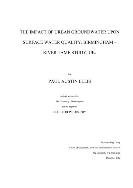
2.1.1 Ground<strong>water</strong> flow to rivers<br />
<strong>The</strong> interaction <strong>of</strong> <strong>ground<strong>water</strong></strong> and <strong>surface</strong> <strong>water</strong> bodies is complex and dependent on many<br />
factors including the topography, geology, climate, and the position <strong>of</strong> the <strong>surface</strong> <strong>water</strong> body<br />
relative to the <strong>ground<strong>water</strong></strong> flow system (Sophocleous, 2002, Winter, 1999 and 2002). Local,<br />
intermediate and/or regional <strong>ground<strong>water</strong></strong> flows may discharge into <strong>surface</strong> <strong>water</strong>s, (Figure<br />
6
REVIEW<br />
2.1) and <strong>surface</strong> <strong>water</strong> may on occasion recharge the <strong>ground<strong>water</strong></strong> (Toth, 1963, Nield et al.,<br />
1994). Hence a reduction in flow or contamination in one will <strong>of</strong>ten affect the other.<br />
Woessner (2000) states that <strong>ground<strong>water</strong></strong> flow to a river channel is dependent on:<br />
1. the distribution and magnitude <strong>of</strong> the hydraulic conductivities within the river channel, the<br />
associated fluvial plain sediments and the underlying bedrock;<br />
2. the relation <strong>of</strong> river stage to the adjacent <strong>ground<strong>water</strong></strong> gradients; and<br />
3. the geometry and position <strong>of</strong> the river channel within the fluvial plain.<br />
Ground<strong>water</strong> is influent to the river channel when the <strong>ground<strong>water</strong></strong> head at the channel<br />
interface is greater than the river stage. Conversely, <strong>surface</strong> <strong>water</strong> is effluent from the channel<br />
when the river stage is higher than the <strong>ground<strong>water</strong></strong> head. Ground<strong>water</strong> through-flow may<br />
occur when the <strong>ground<strong>water</strong></strong> head is higher than the river stage on one bank but lower on the<br />
other (Townley et al., 1992). Ground<strong>water</strong> flow may also occur parallel to the river in which<br />
case only limited <strong>ground<strong>water</strong></strong>/<strong>surface</strong> <strong>water</strong> exchange may occur. During periods <strong>of</strong> high<br />
recharge, <strong>ground<strong>water</strong></strong> ‘mounding’, (ie, rapid increases in head) may occur in the thin<br />
unsaturated zone adjacent to <strong>surface</strong>-<strong>water</strong> bodies which may temporarily influence<br />
<strong>ground<strong>water</strong></strong>/<strong>surface</strong> <strong>water</strong> interactions (Winter, 1983).<br />
A key reference by Winter et al. (1998) summarised the current understanding <strong>of</strong><br />
<strong>ground<strong>water</strong></strong>/<strong>surface</strong> <strong>water</strong> interactions and their relationship to <strong>water</strong> supply, <strong>water</strong> quality<br />
and the aquatic environment, in a variety <strong>of</strong> settings. A unifying framework based on the<br />
concept <strong>of</strong> hydrologic landscapes is used to present conceptual models containing common<br />
7
Abstractions<br />
induce recharge<br />
from <strong>surface</strong><br />
<strong>water</strong>.<br />
Years<br />
River<br />
Days<br />
Flow through<br />
the flood plain<br />
Centuries - Millennia<br />
Ground<strong>water</strong><br />
<strong>surface</strong> <strong>water</strong><br />
exchange<br />
Figure 2.1<br />
Run-<strong>of</strong>f<br />
Ground<strong>water</strong> flow-through Ground<strong>water</strong> influent<br />
Recharge<br />
Aquitard<br />
River gaining River losing<br />
Surface <strong>water</strong> effluent<br />
Figure 2.1 Conceptual model <strong>of</strong> <strong>ground<strong>water</strong></strong> flows to a river
REVIEW<br />
features <strong>of</strong> <strong>ground<strong>water</strong></strong>/<strong>surface</strong> <strong>water</strong> interactions in five general types <strong>of</strong> terrain:<br />
mountainous, riverine, coastal, glacial and dune, and karst.<br />
2.1.2 <strong>The</strong> <strong>ground<strong>water</strong></strong>/<strong>surface</strong> <strong>water</strong> interface<br />
Interactions between <strong>ground<strong>water</strong></strong> and <strong>surface</strong> <strong>water</strong> occur across a transition zone within the<br />
beds <strong>of</strong> lakes, rivers, or seas (Henry, 2002). In the case <strong>of</strong> a river, a ‘hyporheic zone’ develops<br />
where mixing between <strong>ground<strong>water</strong></strong> and <strong>surface</strong> <strong>water</strong> occurs (Biksey et al., 2001). This is an<br />
ecological term that refers to an ecotone where both <strong>ground<strong>water</strong></strong> and <strong>surface</strong> <strong>water</strong> are<br />
present within a stream bed along with a specific set <strong>of</strong> biota (Conant, 2000). <strong>The</strong> flow <strong>of</strong><br />
river <strong>water</strong> over variations in the <strong>surface</strong> <strong>of</strong> the riverbed may cause localised variations in<br />
pressure that induce flow through the riverbed, causing <strong>ground<strong>water</strong></strong>/<strong>surface</strong> <strong>water</strong> mixing<br />
(Figure 2.2). <strong>The</strong> extent <strong>of</strong> this mixing zone may range from centimetres to hundreds <strong>of</strong><br />
meters if <strong>surface</strong> <strong>water</strong> flows through the flood plain sediments are considered (Woessner,<br />
2000, Wroblicky et al., 1998). <strong>The</strong> zone is heterogeneous, dynamic and dependent on the<br />
<strong>surface</strong> <strong>water</strong> and <strong>ground<strong>water</strong></strong> head distribution, river flow, riverbed hydrogeology and<br />
bedform (Fraser et al., 1998).<br />
Large gradients in concentration and environmental conditions <strong>of</strong>ten exist across the transition<br />
zone (Boulton et al., 1998). <strong>The</strong>se affect the spatial and temporal distribution <strong>of</strong> aerobic and<br />
anaerobic microbial processes as well as the chemical form and concentration <strong>of</strong> nutrients,<br />
trace metals and contaminants. Microbial and biological activity may lead to biodegradation<br />
<strong>of</strong> organic contaminants, reducing levels by several orders <strong>of</strong> magnitude within this zone<br />
(Conant, 2000). <strong>The</strong> hyporheic zone is important ecologically because it may store nutrients<br />
(and potentially contaminants), transform compounds biologically and chemically, and<br />
9
(a)<br />
(b)<br />
Ground<strong>water</strong>/<strong>surface</strong> <strong>water</strong><br />
mixing in the hyporheic zone<br />
Ground<strong>water</strong><br />
flow<br />
River Flow<br />
Induced sub<strong>surface</strong><br />
flow <strong>of</strong> river <strong>water</strong><br />
Figure 2.2 Schematic section through a riverbed, (a) longitudinal<br />
(b) lateral (after Winter et al., 1998).<br />
Turbulence<br />
Contaminant plume<br />
with high concentrations<br />
at the core<br />
Riverbed sediments
REVIEW<br />
provide refuge to benthic invertebrates that are the base <strong>of</strong> the aquatic food web (Battin, 1999,<br />
Barnard et al.,1994). Hyporheic organisms are likely to show the effects <strong>of</strong> pollution from<br />
discharging <strong>ground<strong>water</strong></strong> before organisms within the <strong>water</strong> column and so provide an<br />
indicator <strong>of</strong> the <strong>impact</strong> <strong>of</strong> contaminated <strong>ground<strong>water</strong></strong> (Environmental Protection Agency (US),<br />
1998).<br />
Surface <strong>water</strong> exchange and storage within the hyporheic zone influences downstream<br />
nutrient and contaminant transport, and may be associated with enhanced biogeochemical<br />
transformation <strong>of</strong> these compounds in the <strong>surface</strong> <strong>water</strong>. Hyporheic flow paths are typically<br />
small but if rates <strong>of</strong> chemical reactions are rapid enough and the volume <strong>of</strong> exchange great<br />
enough then substantial modifications <strong>of</strong> <strong>surface</strong> <strong>water</strong> quality may occur (Choi et al., 2000,<br />
Packman et al., 2000, Harvey et al., 1993).<br />
2.1.3 Ground<strong>water</strong> contamination<br />
<strong>The</strong> natural background chemistry <strong>of</strong> <strong>ground<strong>water</strong></strong> resulting from recharge composition and<br />
mineral dissolution can be substantially modified by a wide range <strong>of</strong> contaminants that may<br />
be present as different phases within the sub<strong>surface</strong> environment. <strong>The</strong>se include; synthetic<br />
organic compounds, hydrocarbons, metals and other inorganics, and pathogens such as<br />
viruses and bacteria. Conant (2000) summarised the factors that may help to determine the<br />
<strong>impact</strong> <strong>of</strong> a contaminant present in the sub<strong>surface</strong> on a <strong>surface</strong> <strong>water</strong> body. <strong>The</strong>y include:<br />
1. physical and chemical characteristics <strong>of</strong> the contaminants;<br />
2. geometry and temporal variations in the contaminant source;<br />
3. transport mechanisms (advection and dispersion);<br />
4. reactions (reversible and non-reversible).<br />
11
REVIEW<br />
<strong>The</strong> physical and chemical properties <strong>of</strong> the contaminant determine its mobility and toxic<br />
effect. A contaminant may move through the sub<strong>surface</strong> as a pure liquid or gas phase, as a<br />
dissolved phase, in particulate form or attached to colloids. Soluble compounds may be<br />
transported readily within the <strong>ground<strong>water</strong></strong>, and attain high levels <strong>of</strong> concentration. Less<br />
soluble compounds will occur in low concentrations but may provide a long-term source <strong>of</strong><br />
contamination. Advective transport <strong>of</strong> dissolved phase contaminants within the <strong>ground<strong>water</strong></strong><br />
is seen as the primary mechanism by which sub<strong>surface</strong> contaminants may <strong>impact</strong> <strong>upon</strong><br />
<strong>surface</strong> <strong>water</strong> systems.<br />
<strong>The</strong> sources <strong>of</strong> contaminated <strong>ground<strong>water</strong></strong> may be spatially restricted point sources such as an<br />
industrial spill or waste dump, or more diffuse sources such as arise from the widespread<br />
application <strong>of</strong> agricultural fertilisers and pesticides. Point sources tend to give rise to narrow<br />
plumes (Rivett et al., 2001) which migrate with the <strong>ground<strong>water</strong></strong> flow and may eventually<br />
discharge to the <strong>surface</strong> <strong>water</strong> (Figure 2.3). In the USA more than 75% <strong>of</strong> the contaminated<br />
land categorised under the government’s ‘superfund’ sites lie within 0.5 miles <strong>of</strong> a <strong>surface</strong><br />
<strong>water</strong> body and more than half had an <strong>impact</strong> on <strong>surface</strong> <strong>water</strong> in some way (Environmental<br />
Protection Agency (U.S.), 2000).<br />
<strong>The</strong> initial contaminant concentration in the <strong>ground<strong>water</strong></strong> will depend on the mass and<br />
distribution <strong>of</strong> the contaminant in the source area, the rate <strong>of</strong> <strong>ground<strong>water</strong></strong> flow and the<br />
physical-chemical-biological processes controlling contaminant dissolution (Fetter, 1999).<br />
Contaminants derived from the land <strong>surface</strong> may take a considerable time to enter the<br />
<strong>ground<strong>water</strong></strong> if a large unsaturated zone is present. Ground<strong>water</strong> contaminant concentrations<br />
in the source area may vary with time or may give rise to discrete pulse-type inputs.<br />
12
Abstraction<br />
For<br />
drinking<br />
<strong>water</strong><br />
supply<br />
Seepage<br />
face<br />
Hyporheic<br />
zone<br />
Contaminated<br />
tributaries<br />
Surface<br />
<strong>water</strong><br />
exchange<br />
Sediment<br />
grains<br />
Eh.<br />
PH<br />
Temperature<br />
Concentration<br />
Gradients<br />
Diffuse <strong>urban</strong><br />
and agricultural<br />
pollution<br />
Pipe end discharge<br />
Capillary<br />
fringe<br />
Dilution and<br />
dispersion<br />
Leaking<br />
sewers<br />
Converging<br />
<strong>ground<strong>water</strong></strong> flows<br />
Point source<br />
Contaminant plume<br />
Leachate<br />
from<br />
contaminated<br />
land<br />
Natural<br />
mineral<br />
dissolution<br />
Dissolved phase<br />
PROCESSES IN THE RIVERBED<br />
Ground<strong>water</strong> / <strong>surface</strong> <strong>water</strong> mixing<br />
Interstitial transport <strong>of</strong> particulates / colloids<br />
Precipitation / dissolution reaction<br />
Sorption and ion exchange<br />
Line source<br />
LNAPL<br />
Bacterial activity may;<br />
consume nutrients and oxygen, mediate redox<br />
reactions biodegrade organic contaminants<br />
Benthic fauna may be affected by contaminants<br />
Figure 2.3 Conceptual model <strong>of</strong> contaminant inputs to a river.<br />
Recharge<br />
+<br />
aerial<br />
contaminant<br />
deposition<br />
Industrial<br />
spills<br />
DNAPL
REVIEW<br />
Contaminant concentrations within the <strong>ground<strong>water</strong></strong> will be modified en route to, and across,<br />
the <strong>ground<strong>water</strong></strong>/<strong>surface</strong> <strong>water</strong> interface. Dispersion will result in spreading and mixing <strong>of</strong> the<br />
contaminant plume with cleaner <strong>ground<strong>water</strong></strong>. However, lateral dispersion within an aquifer is<br />
generally low and the plume remains narrow relative to its length, the highest contaminant<br />
concentrations being within the central core (Rivett et al., 2001). When the plume reaches the<br />
hyporheic zone, more turbulent conditions are likely to exist as the <strong>ground<strong>water</strong></strong> mixes with<br />
the <strong>surface</strong> <strong>water</strong> and is ultimately diluted in the <strong>surface</strong>-<strong>water</strong> column.<br />
During transport, the contaminants may undergo reversible reactions such as adsorption,<br />
precipitation/dissolution and ion exchange, and non-reversible reactions such as<br />
biodegradation. Reactions may be reversible only under certain conditions. For example<br />
desorption <strong>of</strong> heavy metals occurs under conditions <strong>of</strong> low pH, and therefore contaminants<br />
may be effectively removed from the system until conditions change. <strong>The</strong> types <strong>of</strong> reactions<br />
that occur are dependent on the local conditions, and these may vary considerably along the<br />
contaminant flow path from the source area, through the aquifer to the <strong>ground<strong>water</strong></strong>/<strong>surface</strong><br />
<strong>water</strong> interface. <strong>The</strong>re are key processes controlling the movement and transport <strong>of</strong><br />
contaminants across the <strong>ground<strong>water</strong></strong>/<strong>surface</strong> <strong>water</strong> interface.<br />
1. Bacterial action which may play an important role in catalysing reactions (e.g. sulphate<br />
and nitrate reduction) and directly degrading some organic compounds. <strong>The</strong><br />
<strong>ground<strong>water</strong></strong>/<strong>surface</strong> <strong>water</strong> interface <strong>of</strong>ten has a high nutrient content and anoxic<br />
conditions which are conducive to bacterial action.<br />
2. Adsorption <strong>of</strong> contaminants to sites on the surrounding aquifer material. This reaction is<br />
generally reversible in which case it will not alter the total mass flux <strong>of</strong> the contaminants<br />
but it may significantly retard their transport allowing extra time for other processes to<br />
14
REVIEW<br />
occur such as biodegradation. For organic contaminants, the degree <strong>of</strong> sorption is <strong>of</strong>ten<br />
proportional to the content <strong>of</strong> organic carbon which is generally much higher in the<br />
riverbed sediments relative to the surrounding geology (Schwarzenbach et al., 1981). For<br />
inorganic contaminants, clay minerals, organic matter and oxides/hydroxides all have a<br />
sorption and exchange capacity which may retard contaminant transport (Appelo and<br />
Postma, 1999).<br />
3. Rapid changes in pH, Eh, and mixing <strong>of</strong> <strong>water</strong>s <strong>of</strong> significantly differing concentrations<br />
occur across the <strong>ground<strong>water</strong></strong>/<strong>surface</strong> <strong>water</strong> interface. Ground<strong>water</strong> chemistry which may<br />
have been in equilibrium will adjust rapidly to the new conditions, perhaps leading to<br />
sudden mineral precipitation. Iron oxides are a common example <strong>of</strong> precipitation occuring<br />
when acidic, oxygen-poor <strong>ground<strong>water</strong></strong> mixes with higher pH, more highly oxygenated<br />
<strong>surface</strong> <strong>water</strong>s.<br />
Contaminant movement and transformation across the <strong>ground<strong>water</strong></strong>/<strong>surface</strong> <strong>water</strong> interface<br />
are poorly understood. In light <strong>of</strong> this a workshop was held to summarise the existing<br />
knowledge base on the <strong>ground<strong>water</strong></strong>/<strong>surface</strong> <strong>water</strong> interface and to develop strategies for an<br />
improved understanding <strong>of</strong> the effect <strong>of</strong> contaminated <strong>ground<strong>water</strong></strong> discharge through it. <strong>The</strong><br />
proceedings <strong>of</strong> this workshop provide a key reference on this subject area (Environmental<br />
Protection Agency (U.S.), 2000).<br />
It is predicted that by 2010, half the world’s population <strong>of</strong> 6,500 million will live in towns or<br />
cities, and that much <strong>of</strong> the <strong>urban</strong> growth will be in developing countries (Morris, 2002).<br />
Increasing demand will be placed on both <strong>urban</strong> <strong>ground<strong>water</strong></strong> and <strong>surface</strong> <strong>water</strong> resources for<br />
domestic and industrial use. Unfortunately, <strong>urban</strong> growth is <strong>of</strong>ten associated with degradation<br />
15
REVIEW<br />
<strong>of</strong> <strong>water</strong> quality which limits the usefulness <strong>of</strong> both <strong>ground<strong>water</strong></strong> and <strong>surface</strong> <strong>water</strong> resources<br />
(Petts et al., 2002). <strong>The</strong> occurrence <strong>of</strong> contaminated <strong>ground<strong>water</strong></strong> related to <strong>urban</strong>isation is<br />
well known, both in the U.K. (Barrett et al., 1997, Lerner et al., 1996, Ford et al., 1994, Rivett<br />
et al., 1990) and abroad (Eiswirth et al., 1997, Kacaroglu et al., 1997, Appleyard, 1995).<br />
Likewise, the occurrence <strong>of</strong> poor quality <strong>urban</strong> <strong>surface</strong> <strong>water</strong>s is extremely common<br />
(Kayabalý et al., 1999, Ziegler et al., 2001). However, <strong>urban</strong> <strong>ground<strong>water</strong></strong> and <strong>surface</strong> <strong>water</strong><br />
interactions are less well understood.<br />
2.2 International Case Studies<br />
To characterise the <strong>impact</strong> <strong>of</strong> <strong>urban</strong> <strong>ground<strong>water</strong></strong> on <strong>surface</strong>-<strong>water</strong> quality requires a broad<br />
multidisciplinary approach involving hydrological, hydrogeological, hydrochemical and<br />
ecological elements. To cover all these elements is generally beyond the scope <strong>of</strong> a single<br />
study and previous work has <strong>of</strong>ten focussed on a particular <strong>ground<strong>water</strong></strong> and/or <strong>surface</strong> <strong>water</strong><br />
flow and/or quality issue. <strong>The</strong> scale <strong>of</strong> the studies can be divided into those that provide<br />
detailed but localised information on a specific contaminant plume or process across the river<br />
bed, and those that provide more general regional information on <strong>surface</strong>-<strong>water</strong> quality and<br />
flow. Only limited work has been done on scaling up the effects <strong>of</strong> local processes to the<br />
catchment scale. <strong>The</strong> <strong>urban</strong> <strong>ground<strong>water</strong></strong> system generally lies between these two extremes <strong>of</strong><br />
scale, having many potential contaminant sources but covering a limited extent <strong>of</strong> the total<br />
catchment area.<br />
16
2.2.1 Water quality studies<br />
REVIEW<br />
Relationships between <strong>ground<strong>water</strong></strong> and <strong>surface</strong>-<strong>water</strong> quality have been investigated for<br />
nutrients, pesticides , volatile organic compounds and metals (Lindsey et al., 1998, Bevans et<br />
al., 1998). A major study <strong>of</strong> the <strong>surface</strong> <strong>water</strong> and <strong>ground<strong>water</strong></strong> quality in the Potomac River<br />
Basin, USA, revealed a substantial <strong>impact</strong> from anthropogenic sources <strong>of</strong> contamination<br />
related to <strong>urban</strong>isation (Ator et al., 1998). Chlorodane, DDT, PCBs, mercury and lead were all<br />
detected in streambed sediment and aquatic tissues derived from persistent sources, such as<br />
<strong>ground<strong>water</strong></strong>, within the river basin. Grischek et al. (1996) investigated <strong>urban</strong> <strong>ground<strong>water</strong></strong><br />
quality beneath the city <strong>of</strong> Dresden in Germany and found the influent <strong>surface</strong> <strong>water</strong> from the<br />
River Elbe to have only a limited effect. Hartwell (1997) investigated the transport <strong>of</strong> the<br />
herbicide atrazine between the Cedar River and <strong>ground<strong>water</strong></strong> in Iowa, USA. <strong>The</strong> study found<br />
that <strong>ground<strong>water</strong></strong> from the adjacent alluvial aquifer was the principal source <strong>of</strong> atrazine in the<br />
river during base-flow conditions.<br />
Lorah et al. (1999) and Conant (2000) investigated the discharge <strong>of</strong> chlorinated solvent<br />
plumes to <strong>surface</strong> <strong>water</strong> systems and found evidence for enhanced biodegradation across the<br />
interface. Schwarzenbach et al. (1981) conducted some <strong>of</strong> the earliest work on<br />
<strong>ground<strong>water</strong></strong>/<strong>surface</strong> <strong>water</strong> contaminant interactions based on laboratory simulations <strong>of</strong> field<br />
conditions beneath a river valley in Switzerland. <strong>The</strong>y conducted a ‘classic’ set <strong>of</strong> sorption<br />
studies and showed sorption to organic carbon to be a key process in retarding the transport <strong>of</strong><br />
non-polar organic compounds across the <strong>ground<strong>water</strong></strong>/<strong>surface</strong> <strong>water</strong> interface.<br />
Metal contamination resulting from acidic <strong>ground<strong>water</strong></strong> associated with mining activities has<br />
been widely researched (Benner et al., 1995, Kimball et al., 2002). Paulson (1997)<br />
17
REVIEW<br />
investigated the transport and fate <strong>of</strong> Fe, Mn, Cu, Zn, Cd, Pb and SO4 in a <strong>ground<strong>water</strong></strong> plume<br />
and in the downstream <strong>surface</strong> <strong>water</strong>s in the Coeur d’Alene Mining District in the US. He<br />
found that <strong>upon</strong> mixing with higher pH <strong>surface</strong> <strong>water</strong> the metals were lost from solution in the<br />
following order: Fe>Al>Pb>Cu>Mn>Zn> Cd. Less than 10% <strong>of</strong> the dissolved Zn and Cd<br />
were lost, despite a 5 km journey through both the <strong>ground<strong>water</strong></strong> and <strong>surface</strong> <strong>water</strong> regimes.<br />
Paulson and Balistrieri (1999) used model simulations and laboratory experiments to examine<br />
the removal <strong>of</strong> Cd, Cu, Pb and Zn in acidic <strong>ground<strong>water</strong></strong> during neutralisation by ambient<br />
<strong>surface</strong> <strong>water</strong>s. <strong>The</strong>y concluded that hydrous Fe oxides and particulate organic carbon are<br />
more important than hydrous Al oxides in removing metals from the <strong>ground<strong>water</strong></strong>. Tessier et<br />
al. (1996) found that trace metals present in <strong>water</strong> influent to two lakes in Canada sorbed<br />
directly to the OH functional groups <strong>of</strong> iron and manganese oxyhroxides and organic matter<br />
found in the lake sediments. Kuwabara et al. (1999) found that <strong>water</strong> flowing through the bed<br />
<strong>of</strong> lake Coeur d’Alene caused a significant flux <strong>of</strong> metal from the lake sediments to the <strong>water</strong><br />
column.<br />
2.2.2 Flow Studies<br />
<strong>The</strong> <strong>ground<strong>water</strong></strong> support <strong>of</strong> river baseflow and its relationship to the underlying geology has<br />
has long been recognised and studied (Meyboom, 1961, Mau et al., 1993, Pinder et al., 1969,<br />
O’Conner 1976,). Several studies have investigated the relationship between reduced <strong>surface</strong><br />
<strong>water</strong> flows and increased levels <strong>of</strong> <strong>ground<strong>water</strong></strong> abstraction (Sophocleous 2000). A<br />
comprehensive study on the interaction <strong>of</strong> the Equus Beds alluvial aquifer and the Arkansas<br />
River, USA, found that abstraction for irrigation significantly reduced river baseflow levels<br />
and induced <strong>surface</strong> <strong>water</strong> seepage into the aquifer (Ziegler et al., 2001). <strong>The</strong> response <strong>of</strong><br />
<strong>ground<strong>water</strong></strong> to transient <strong>surface</strong> <strong>water</strong> levels has been used to derive estimates <strong>of</strong> the aquifer<br />
property S/T (Reynolds, 1987, Workman et al., 1997, Erskine 1991). Devito et al. (1996)<br />
18
REVIEW<br />
investigated <strong>ground<strong>water</strong></strong>/<strong>surface</strong> <strong>water</strong> interactions and the <strong>ground<strong>water</strong></strong> contribution to<br />
wetlands on the Canadian Shield and demonstrated the control <strong>of</strong> morphology and shallow<br />
sub<strong>surface</strong> geology on the hydrology <strong>of</strong> valley bottom swamps. Wroblicky et al. (1998)<br />
investigated the <strong>ground<strong>water</strong></strong> flow and seasonal variations in the hyporheic zone for two first<br />
order mountain streams in the US. <strong>The</strong> streams were in alluvial material with different<br />
hydraulic properties derived from bedrock types comprising welded tuff and sandstone.<br />
Numerical modelling was used to simulate unconfined transient flow. Sensitivity analyses<br />
indicated that changes in the hydraulic conductivity <strong>of</strong> the alluvial and streambed sediments<br />
and variation in recharge rates have greatest <strong>impact</strong> on the magnitude, direction, and spatial<br />
distribution <strong>of</strong> stream/<strong>ground<strong>water</strong></strong> exchange.<br />
2.2.3 Combined Quality and Flow Studies<br />
Case studies <strong>of</strong> <strong>ground<strong>water</strong></strong>/<strong>surface</strong> <strong>water</strong> quality and flow interactions have generally been<br />
conducted in a rural setting (Cey et al., 1998, Pionke et al., 1998) in order to avoid the<br />
complexities associated with <strong>urban</strong> rivers which have many inputs (Ellis et al., 2002,<br />
Appendix 1). Gburek et al. (1999) investigated the flow and major ion contributions to<br />
baseflow in an upland <strong>water</strong>shed in Canada. <strong>The</strong> study showed increased ionic concentrations,<br />
including nitrate, within <strong>ground<strong>water</strong></strong> baseflow derived from an area <strong>of</strong> agricultural land<br />
compared with low ionic concentrations from forested areas. A chemical mass balance (i.e<br />
concentration x flow) was used to investigate the contribution <strong>of</strong> <strong>ground<strong>water</strong></strong> from different<br />
parts <strong>of</strong> the study area. A simple model was developed based on land use to explain nitrate<br />
concentrations within baseflow.<br />
Diffuse nitrate pollution <strong>of</strong> <strong>surface</strong> <strong>water</strong>s from <strong>ground<strong>water</strong></strong> has been investigated in several<br />
studies in the USA (MacNish et al., 1998). (Bachman et al., 1997) used river baseflow<br />
analyses and <strong>surface</strong> <strong>water</strong> quality sampling to calculate nitrate loading to Chesapeake Bay.<br />
19
REVIEW<br />
<strong>The</strong> median <strong>ground<strong>water</strong></strong> contribution was estimated as 56% <strong>of</strong> the total nitrate load under<br />
baseflow. Harvey et al. (1998) examined the effect <strong>of</strong> enhanced maganese oxidation (and co-<br />
precipitation <strong>of</strong> trace metals) in the hyporheic zone on basin-scale geochemical mass balance<br />
in a drainage basin contaminated by copper mining.<br />
2.3 UK Case Studies<br />
Published data on <strong>ground<strong>water</strong></strong> quality and flow interactions in the UK are generally limited.<br />
A few <strong>of</strong> the key studies are briefly presented.<br />
A study <strong>of</strong> trace-element concentrations in the major rivers entering the Humber estuary<br />
showed elevated levels in the rivers draining industrial <strong>urban</strong> catchments (Neal et al., 1996).<br />
<strong>The</strong> relationship between concentration and flow was used to evaluate the sources <strong>of</strong> trace<br />
elements; a negative relationship to flow implied a <strong>ground<strong>water</strong></strong> source. Within the <strong>urban</strong><br />
rivers, most elements in the dissolved phase exhibited negative relationships, indicating that<br />
point-source discharges provided the major source <strong>of</strong> trace elements. Roberts et al. (1998)<br />
investigated nitrate contamination <strong>of</strong> <strong>ground<strong>water</strong></strong> in the Lincolnshire Limestone resulting<br />
from <strong>surface</strong> <strong>water</strong> recharge related to local <strong>ground<strong>water</strong></strong> abstractions.<br />
Of particular concern in the UK has been the widespread detection <strong>of</strong> pesticides at low levels<br />
within <strong>ground<strong>water</strong></strong>s and <strong>surface</strong> <strong>water</strong>s (Croll, 1991). Clark et al. (1991) investigated<br />
pesticide occurrence in the River Granta and the underlying <strong>ground<strong>water</strong></strong> within the chalk<br />
aquifer <strong>of</strong> Cambridgeshire. <strong>The</strong> maximum levels <strong>of</strong> pesticide were found in the river during<br />
periods <strong>of</strong> high flow. However, even under low-flow conditions, levels <strong>of</strong> pesticide were<br />
persistent and are probably derived from the <strong>ground<strong>water</strong></strong>. Of particular interest in the study,<br />
20
REVIEW<br />
owing to their widespread detection and/or application, were the pesticides atrazine, simazine,<br />
isoproturon, chlortoluron and tri-allate.<br />
Hooda et al. (1997) found the <strong>impact</strong> <strong>of</strong> diffuse phosphorous loading on six small catchments<br />
in Scotland to be greatest during summer <strong>ground<strong>water</strong></strong>-fed baseflow conditions. Birtles,<br />
(1978) modelled <strong>water</strong> quality in the River Severn by separating the river hydrographs into<br />
discrete components each <strong>of</strong> which had separate, conservative, <strong>surface</strong> <strong>water</strong> quality<br />
parameters. <strong>The</strong>se comprised, direct run-<strong>of</strong>f, baseflow from the Triassic Sandstone deposits,<br />
baseflow from superficial deposits and effluent returns. Younger et al. (1993) investigated<br />
<strong>ground<strong>water</strong></strong>/<strong>surface</strong> <strong>water</strong> interactions in the Thames basin.<br />
Research currently in progress in the UK is summarised by Young et al. (2002). New research<br />
initiatives are under way to provide support for integrated <strong>ground<strong>water</strong></strong>/<strong>surface</strong> <strong>water</strong><br />
monitoring and assessment for sustainable catchment management. <strong>The</strong>se include the<br />
Lowland Catchment Research Programme, LOCAR, (Peach et al., 2000, LOCAR, 2002) and<br />
the Catchment Hydrology and Sustainable Management (CHASM) group which will<br />
investigate highland catchments (CHASM, 2002). <strong>The</strong> recently concluded Land-Ocean<br />
Interaction Study (LOIS, 1998) was undertaken to quantify the chemical fluxes entering the<br />
North Sea from the surrounding countries, including the UK. Extensive data sets were<br />
collected for the Humber catchment which incorporate the <strong>ground<strong>water</strong></strong> contribution to the<br />
total geochemical flux to the sea. Most <strong>of</strong> the current research is focussed on rural catchments<br />
and there is a lack <strong>of</strong> ongoing research into <strong>urban</strong> <strong>ground<strong>water</strong></strong>/<strong>surface</strong> <strong>water</strong> interactions.<br />
21
2.3.1 UK Legislation<br />
REVIEW<br />
<strong>The</strong> new Water Framework Directive (Council <strong>of</strong> Europe, 2000, Environment Agency, 2002)<br />
has been introduced to ensure an integrated approach to the management <strong>of</strong> catchment <strong>surface</strong><br />
and <strong>ground<strong>water</strong></strong> quality and flow. Consultations are under way in the UK on the<br />
implementation <strong>of</strong> this directive (DEFRA, 2002). It will be implemented in conjunction with<br />
other legislation such as Part IIa <strong>of</strong> the Environmental Protection Act 1990 designed to<br />
maintain and improve the quality <strong>of</strong> <strong>surface</strong> and <strong>ground<strong>water</strong></strong>. Under the legislation, the<br />
<strong>impact</strong> <strong>of</strong> land causing pollution <strong>of</strong> controlled <strong>water</strong>s must be assessed by comparison to the<br />
background <strong>water</strong> quality and suitable standards such as drinking <strong>water</strong> and environmental<br />
quality standards (EQS) for <strong>surface</strong> <strong>water</strong>s (Smith, 2002). Contaminated land and<br />
contaminated <strong>ground<strong>water</strong></strong>s arising, where found to cause significant <strong>impact</strong>s on the <strong>surface</strong><br />
<strong>water</strong> are likely to require remedial action (Rivett et al., 2002).<br />
2.4 Monitoring methods<br />
Comprehensive reviews <strong>of</strong> the existing analytical, numerical, field and chemical investigative<br />
techniques for <strong>ground<strong>water</strong></strong>/<strong>surface</strong> <strong>water</strong> interactions have been carried out by HRU (2001)<br />
and Winter (1995). On the catchment scale, the most widely-used approach is river<br />
hydrograph separation and baseflow recession analyses to derive the <strong>ground<strong>water</strong></strong> component<br />
<strong>of</strong> river flow (Meyboom, 1961, Mau et al., 1997, Gustard et al., 1992). Several workers<br />
(Pinder et al., 1969, O’Conner 1976, Birtles 1978) have used differences in <strong>ground<strong>water</strong></strong> and<br />
<strong>surface</strong> <strong>water</strong> chemistry and total dissolved solids to resolve further the <strong>ground<strong>water</strong></strong><br />
component <strong>of</strong> the river hydrographs. At the smaller scale <strong>of</strong> the river reach, stream tracers<br />
22
REVIEW<br />
have been used to determine river discharge accretion and characterise river sub<strong>surface</strong> <strong>water</strong><br />
exchange (Harvey et al., 1996, Kimball, 2002).<br />
Piezometers and piezometer nests have been used in several studies to obtain <strong>water</strong> samples<br />
and head measurements within the <strong>ground<strong>water</strong></strong>/<strong>surface</strong> <strong>water</strong> interface (Dean et al., 1999,<br />
Cey et al., 1998, Lee, 1980, Henry, 2000). Other in situ sampling devices have also been<br />
developed such as the colonisation corer (Fraser et al., 1996) and the bead tube sampler<br />
(Moore, 2000). Passive sampling techniques based on diffusive gradients across semi-<br />
permeable membrane devices have been used to detect both hydrophobic organics and heavy<br />
metals in aquatic environments (Vroblesky et al., 1997; Church et al., 2000). A number <strong>of</strong><br />
devices have been developed to measure the seepage across a lake or riverbed (Lee, 1977;<br />
Carr et al., 1980; Isiorho, 1999) although the methods <strong>of</strong>ten encounter errors when used in<br />
fast-flowing river environments (Libelo et al., 1994). <strong>The</strong> temperature gradient across the<br />
<strong>ground<strong>water</strong></strong>/<strong>surface</strong> <strong>water</strong> interface has been used to determine flow rates (Silliman et al.,<br />
1995, Evans et al. 1997). Several <strong>of</strong> the investigative methods identified in the literature<br />
review were adapted for use in the present study.<br />
2.5 Modelling methods<br />
A review <strong>of</strong> analytical and numerical methods <strong>of</strong> modelling river-aquifer interactions are<br />
presented by HRU (2001), Winter (1995) and Younger (1989). Analytical solutions have been<br />
developed from early simulations <strong>of</strong> 1D <strong>ground<strong>water</strong></strong> interaction with fully penetrating<br />
streams (Rorabaugh, 1964) to meet a range <strong>of</strong> applications. <strong>The</strong>se include the simulation <strong>of</strong><br />
bank storage and <strong>ground<strong>water</strong></strong> fluctuations during river flood events (Serrano and Workman,<br />
23
REVIEW<br />
1998, Reynolds, 1987, Hunt, 1990), travel times for <strong>surface</strong> <strong>water</strong> into contiguous aquifers<br />
(Heij, 1989) and the effects <strong>of</strong> pumping <strong>ground<strong>water</strong></strong> on stream flow (Spalding et al., 1991).<br />
<strong>The</strong> onset <strong>of</strong> readily available computing power has led to an increase in the use <strong>of</strong> numerical<br />
models to simulate <strong>ground<strong>water</strong></strong>/<strong>surface</strong> <strong>water</strong> interactions. <strong>The</strong>se have been successfully<br />
applied to numerous field studies for different hydrogeologic settings and scales (Modica,<br />
1993, Jorgensen et al., 1989, Younger, 1989, Rushton et al., 1989, Sophocleous, 1991). Most<br />
models use idealised stream geometry and the Darcy equation to simulate transfer <strong>of</strong> <strong>water</strong><br />
across the streambed sediments. In this case <strong>ground<strong>water</strong></strong> discharge = hydraulic conductivity<br />
x hydraulic gradient x cross sectional area. This may <strong>of</strong>ten be an oversimplification <strong>of</strong> the<br />
natural system. Previous workers (Rushton et al., 1979) indicate that the relationship between<br />
discharge and hydraulic gradient is not always linear, with variations occurring in the<br />
hydraulic conductivity, particularly if flow reversal occurs. Near <strong>surface</strong> <strong>water</strong> bodies,<br />
convergent flow with a considerable vertical component <strong>of</strong>ten occurs which must be<br />
accounted for if hydraulic conductivity is anisotropic.<br />
<strong>The</strong> realistic simulation <strong>of</strong> transient <strong>surface</strong> <strong>water</strong> flows and <strong>ground<strong>water</strong></strong> flows across a<br />
region is complex. Surface <strong>water</strong> and <strong>ground<strong>water</strong></strong> flow equations may be coupled and solved<br />
simultaneously by iteration. However, more commonly the <strong>surface</strong> <strong>water</strong> heads are set (from<br />
field data or separate modelling) or river baseflow is determined as output from a<br />
<strong>ground<strong>water</strong></strong> model (Younger, 1989). <strong>The</strong> widely used <strong>ground<strong>water</strong></strong> flow model MODFLOW<br />
(Macdonald and Harbaugh, 1988) has been adapted to incorporate a 1D simulation <strong>of</strong><br />
unsteady flow in open-channel networks, but still utilises the simple Darcy equation for <strong>water</strong><br />
transfer. Other models have been developed to investigate <strong>ground<strong>water</strong></strong>/<strong>surface</strong> <strong>water</strong><br />
interaction for variably saturated <strong>ground<strong>water</strong></strong> systems for losing streams (Riesenauer, 1963)<br />
24
REVIEW<br />
and under conditions <strong>of</strong> non-uniform recharge adjacent to a <strong>surface</strong> <strong>water</strong> body (Winter, 1983,<br />
Cooley 1983). Models have been used to evaluate the effect <strong>of</strong> <strong>ground<strong>water</strong></strong> pumping on<br />
stream flow for <strong>water</strong> resources and environmental <strong>impact</strong> purposes (Sophocleous, 2000,<br />
Eberts and Blair, 1990). Flow and transport modelling has been used to investigate solute<br />
(contaminant) transfer between <strong>ground<strong>water</strong></strong> and <strong>surface</strong> <strong>water</strong> on the regional scale (Duffy<br />
and Lee, 1992, Jakeman et al., 1989). Geochemical models such as the USGS model<br />
PHREEQC have been used to simulate solute fate and transport across the<br />
<strong>ground<strong>water</strong></strong>/<strong>surface</strong> <strong>water</strong> interface (Van Breukelen et al., 1998).<br />
2.6 Conclusions<br />
Ground<strong>water</strong>/<strong>surface</strong> <strong>water</strong> quality and flow interactions are complex and variable between<br />
and within catchments. Further work is required to better understand the link between quality<br />
and flow processes, particularly in an <strong>urban</strong> setting where research to date has been limited.<br />
<strong>The</strong> <strong>ground<strong>water</strong></strong>/<strong>surface</strong> <strong>water</strong> interface is ecologically important and is a major pathway for<br />
mass transfer between the sub<strong>surface</strong> and <strong>surface</strong>. Contaminant and nutrient concentrations<br />
within both the <strong>ground<strong>water</strong></strong> and <strong>surface</strong> <strong>water</strong> may be altered significantly during their<br />
passage through the <strong>ground<strong>water</strong></strong>/<strong>surface</strong> <strong>water</strong> interface. <strong>The</strong> interface <strong>of</strong>ten shows high<br />
environmental and concentration gradients. Significant processes that occur across this zone<br />
that may affect contaminant fate and transport include; sorption and precipitation reactions<br />
and bacterial activity which may mediate chemical reactions and degrade organic<br />
contaminants. <strong>The</strong> key references identified in the review <strong>of</strong> <strong>ground<strong>water</strong></strong>-<strong>surface</strong> interactions<br />
were, Sophocleous (2002), Winter et al. (1998), EPA (2000), and Woessner (2000). Useful<br />
case studies <strong>of</strong> <strong>ground<strong>water</strong></strong> quality and flow interactions were Cey et al. (1998) and Gburek<br />
et al. (1999).<br />
25
CHAPTER 3. STUDY SETTING<br />
STUDY SETTING<br />
<strong>The</strong> River Tame drains a 408 km 2 highly <strong>urban</strong>ised catchment covering part <strong>of</strong> the West<br />
Midlands conurbation, which currently supports a population in excess <strong>of</strong> 1.8 million, and<br />
includes Birmingham the UK’s second largest city. <strong>The</strong> Tame forms part <strong>of</strong> the larger<br />
drainage system <strong>of</strong> the River Trent, which eventually drains to the North Sea. It rises to the<br />
east <strong>of</strong> a ridge that forms part <strong>of</strong> the major <strong>water</strong>shed <strong>of</strong> central England with the River Stour<br />
in the Severn catchment to the west draining to the Bristol Channel. <strong>The</strong> three upper arms <strong>of</strong><br />
the Tame (Figure 3.1) rise in the ‘Black Country’ towns <strong>of</strong> Wolverhampton, Walsall and<br />
Oldbury before joining to flow eastwards through the northern part <strong>of</strong> Birmingham. <strong>The</strong> river<br />
baseflow is supported by contributions from sewage effluent and other industrial discharges<br />
plus a significant contribution from <strong>ground<strong>water</strong></strong> which may increase the flow by >20%<br />
across the research area. <strong>The</strong> 24 km study reach lies between the gauging stations <strong>of</strong> Bescot<br />
and Water Orton and work has been focused on the central 7.4 km section that overlies the<br />
unconfined Birmingham Aquifer.<br />
3.1 Historical Background<br />
<strong>The</strong> West Midlands conurbation has been a population centre for the past 200 years and a<br />
major centre for heavy industry since the industrial revolution. Rapid development <strong>of</strong> the area<br />
occurred during the industrial revolution based on the exploitation and processing <strong>of</strong> raw<br />
materials from the South Staffordshire Coal Field and local ironstone deposits. A series <strong>of</strong><br />
canals (from 1800) and later railways (from 1840) were constructed connecting various<br />
26
(b)<br />
(a)<br />
River Tame<br />
10 m<br />
topographic<br />
contours<br />
Motorway<br />
Railway<br />
Regional<br />
Study Reach<br />
Detailed<br />
Study Reach<br />
Figure 3.1 (a) Catchment map <strong>of</strong> the Upper Tame (b) Topography <strong>of</strong> the detailed study<br />
reach (c) Regional Setting<br />
(c)
STUDY SETTING<br />
sections <strong>of</strong> the city with the rest <strong>of</strong> the country and facilitating the rapid growth and spread <strong>of</strong><br />
<strong>urban</strong>isation. <strong>The</strong> sparsely populated semi-rural area was transformed into a series <strong>of</strong><br />
gradually expanding towns that have eventually coalesced to form the West Midlands<br />
conurbation. <strong>The</strong> region became a major centre for metal working and manufacturing<br />
industries with productivity reaching maximum levels during the two world wars. Because <strong>of</strong><br />
this development, a large demand was placed on both <strong>surface</strong> <strong>water</strong> and <strong>ground<strong>water</strong></strong><br />
resources for industrial and public supply.<br />
Contamination <strong>of</strong> soils, <strong>ground<strong>water</strong></strong> and <strong>surface</strong> <strong>water</strong> occurred as a result <strong>of</strong> the <strong>urban</strong>isation<br />
with little or no legislation in place to control it. This pollution combined with sewage<br />
effluent and industrial discharges began to seriously effect river quality during the 19 th<br />
Century. By 1870 Birmingham City had major problems with the disposal <strong>of</strong> sewage effluent<br />
and the continued deterioration <strong>of</strong> <strong>water</strong> quality in the Tame prompted the construction <strong>of</strong> the<br />
Elan Valley reservoirs in Mid Wales to achieve an adequate public supply. This had the effect<br />
<strong>of</strong> increasing flow in the Tame which received the increased levels <strong>of</strong> sewage effluent.<br />
Because <strong>of</strong> overloading <strong>of</strong> the sewerage system untreated effluents <strong>of</strong>ten entered the river and<br />
by 1918 the Tame supported no fish life and by 1945 virtually no aquatic life (Clay, 2000).<br />
Today, the Tame, which once supported salmon and trout has no sustainable fish population<br />
in the study area (Crabtree et al., 1998). Ground<strong>water</strong> quality in the Birmingham Aquifer also<br />
showed a substantial deterioration with many public supply wells polluted and abandoned by<br />
1920 (Greswell et al., 2000).<br />
Since the 1950s’ modification <strong>of</strong> the sewerage system, a reduction in heavy industry and the<br />
implementation <strong>of</strong> better pollution control has helped to improve the <strong>surface</strong> <strong>water</strong> quality.<br />
28
STUDY SETTING<br />
But under the General Quality Assessment (Environment Agency, 1998) the Tame is still<br />
categorised within the worst classes E/F (poor/bad) with severe <strong>impact</strong>s reported on the river<br />
ecology. Rapid <strong>urban</strong> run-<strong>of</strong>f from precipitation events can generate high <strong>surface</strong> <strong>water</strong> flows<br />
and large pollutant loads that add to the hostile conditions for aquatic life.<br />
<strong>The</strong> long history <strong>of</strong> industrialisation and <strong>urban</strong>isation has left a legacy <strong>of</strong> contaminated land,<br />
which has caused significant inorganic and more recently organic contamination <strong>of</strong> the<br />
underlying <strong>ground<strong>water</strong></strong>. <strong>The</strong> contribution <strong>of</strong> sewage effluent and industrial pipe end<br />
discharges to the <strong>surface</strong> <strong>water</strong> quality and flow are relatively well understood but little is<br />
known about the contribution <strong>of</strong> <strong>ground<strong>water</strong></strong> across the study reach.<br />
3.2 Land use<br />
Heavy industry and housing grew up side by side with little or no legislation to control<br />
contamination <strong>of</strong> soils, <strong>ground<strong>water</strong></strong> and <strong>surface</strong> <strong>water</strong>.<br />
Studies <strong>of</strong> <strong>urban</strong> <strong>ground<strong>water</strong></strong> pollution throughout the UK (Lerner et al.,1996) and in nearby<br />
Wolverhampton (Bridge et al., 1997) identified associations between particular contaminants<br />
and land use. Sampling <strong>of</strong> the Birmingham Aquifer has identified <strong>ground<strong>water</strong></strong> contamination<br />
including heavy metals and chlorinated solvents associated with industrial land use (Rivett et<br />
al., 1990, Ford et al.,1994). Metal working and related industries which constitute 59% <strong>of</strong> the<br />
industry overlying the Birmingham Aquifer (Rivett et al., 1990.) are thought to be among the<br />
most significant polluters.<br />
A high concentration <strong>of</strong> industry is located in the Tame Valley which is particularly<br />
vulnerable to <strong>ground<strong>water</strong></strong> pollution owing to the limited thickness <strong>of</strong> the drift and the shallow<br />
<strong>water</strong> table. Recent studies (Thomas, 2001) <strong>of</strong> land use on the unconfined Birmingham<br />
29
STUDY SETTING<br />
Aquifer show industry to comprise 19% <strong>of</strong> land use within the Tame Valley adjacent (60 m 3 s -1 (5184 Mld -1 ) at Water Orton (J.West,<br />
2000). Gently undulating terrain surrounds the river as it flows down a relatively shallow<br />
gradient which remains fairly constant along the length <strong>of</strong> the reach at 0.0013. <strong>The</strong> highest<br />
elevation <strong>of</strong> 283 m above<br />
30
(a)<br />
Land Use In <strong>The</strong> River Tame Corridor Across <strong>The</strong> Birmingham Aquifer, Upto 1 Km From Each Bank<br />
(After Thomas, 2001)<br />
(b)<br />
Residential<br />
40%<br />
Railway/transport<br />
0.6%<br />
River<br />
0.4%<br />
Roads<br />
25%<br />
Canal/Reservoir<br />
2%<br />
Cemetery / Graveyard<br />
2%<br />
Park/Open Land<br />
11%<br />
Industrial/Commercial<br />
19%<br />
Figure 3.2 (a) Land use map within 1 km <strong>of</strong> the River Tame, (b) Categorisation <strong>of</strong> land use
STUDY SETTING<br />
Ordnance Datum (maod) occurs to the south west at Romsley Hill and the lowest point <strong>of</strong> 70<br />
maod is at Kingsbury, north <strong>of</strong> the Lea Marston Lakes (Figure 3.1).<br />
<strong>The</strong> river has been extensively modified from its original form as a meandering braided river<br />
system on a broad flood plain. More than 50% <strong>of</strong> the study reach has undergone engineering<br />
works for flood defence purposes, including strengthening bank sides and straightening some<br />
sections <strong>of</strong> the river. <strong>The</strong> channel bottom remains natural and unlined over most <strong>of</strong> its length,<br />
apart from some concrete-lined sections beneath the M6 motorway (Figure 3.3). Some <strong>of</strong> the<br />
tributaries have been brick lined (River Rea) or culverted (Hockley Brook). Bed materials<br />
range from sub angular cobbles through gravel, sand and silt and include many artefacts.<br />
Weed growth within the channel is limited during the winter months but is abundant during<br />
the summer and is thought to have an effect on the hydrological regime by reducing flow<br />
velocities (Clay, 1999).<br />
Aside from <strong>ground<strong>water</strong></strong> discharge, sewage effluent is a major component <strong>of</strong> dry weather flow<br />
in the river, with 55% <strong>of</strong> flow at the Lea Marston Lakes (Figure 3.1) attributed to sewage<br />
discharge. Efforts to improve the <strong>surface</strong> <strong>water</strong> quality have led to the closure <strong>of</strong> some <strong>of</strong> the<br />
smaller sewage treatment works (STWs) and the centralisation <strong>of</strong> treatment at larger plants.<br />
Several STWs discharge upstream <strong>of</strong> the study area and one within it, at Rayhall (Figure<br />
3.1a), which is intended to operate at a constant discharge <strong>of</strong> 30 Mld -1 . Sewage in excess <strong>of</strong><br />
this capacity is transported from Rayhall to Minworth STW, by the recently constructed Black<br />
Country Trunk sewer, and discharged downstream <strong>of</strong> Water Orton. <strong>The</strong> STWs are a major<br />
control on the <strong>surface</strong> <strong>water</strong> flow balance and the <strong>water</strong> quality within the river and introduce<br />
a significant temporal variability to both. <strong>The</strong> daily fluctuation in <strong>surface</strong> <strong>water</strong> flows related<br />
32
(a)<br />
(b)<br />
Figure 3.3 (a) Photograph <strong>of</strong> the River Tame by the M6 Motorway, (b) Installation <strong>of</strong> riverbed<br />
piezometers.
STUDY SETTING<br />
to the STW takes ~6 hours to propagate from Bescot to Water Orton. A rhodamine dye tracer<br />
experiment (Clay, 2000) undertaken along the study reach showed an overall travel time <strong>of</strong> 20<br />
hours (0.33 msec -1 ) for the dye between Bescot and Water Orton.<br />
3.4 <strong>The</strong> Geology <strong>of</strong> the Tame Catchment<br />
<strong>The</strong> River Tame rises in the west on the Carboniferous Middle Coal Measures and flows<br />
eastwards across the Silurian Wenlock Shale and the Upper Coal Measures before reaching an<br />
unconformable contact with the Triassic Sandstone <strong>of</strong> the Birmingham Aquifer. <strong>The</strong> Tame<br />
continues to flow eastwards for 7.3 km over the sandstone (Figures 3.4 and 3.5) crossing the<br />
Birmingham fault onto the down-thrown Mercia Mudstone which form the eastern division<br />
<strong>of</strong> the study area. Outcrops are rare (Figure 3.6) and the bedrock is generally covered by<br />
superficial drift deposits <strong>of</strong> glacial and alluvial origin (Figure 3.7) ranging in thickness from 1<br />
to 40 m. <strong>The</strong> principal focus <strong>of</strong> the study is related to the interaction <strong>of</strong> the river with the<br />
underlying Triassic Sandstone <strong>of</strong> the Birmingham Aquifer.<br />
Information on the solid and drift geology was derived from recent geological maps and<br />
memoirs (Powell et al.,2000) <strong>of</strong> the British Geological Survey and a study <strong>of</strong> rising<br />
<strong>ground<strong>water</strong></strong> levels within the Birmingham Aquifer (Knipe et al.,1993). <strong>The</strong>se data summarise<br />
a considerable body <strong>of</strong> earlier work combined with more recent mapping. Owing to the<br />
extensive <strong>urban</strong> land cover and the lack <strong>of</strong> outcrop in the study area, the geology (Table 3.1)<br />
is based in large part on the interpretation <strong>of</strong> <strong>water</strong>-well borehole logs and site investigation<br />
reports.<br />
34
Figure 3.4 Schematic geology <strong>of</strong> the study area<br />
Figure 3.5 Schematic geological cross <strong>of</strong> the study area (Jackson et al., 1983)
Study Area<br />
Figure 3.6 Solid geology <strong>of</strong> the Tame catchment (Powell et al., 2000)<br />
Figure 3.7 Drift and solid geology across the unconfined Birmingham Aquifer (Thomas, 2001)
Table 3.1 Description <strong>of</strong> geological units<br />
Age and Unit Description<br />
RECENT<br />
Made Ground<br />
Comprising mine spoil, sand and gravel mixtures <strong>of</strong>ten<br />
with substantial quantities <strong>of</strong> ash and slag and rubble.<br />
1-6<br />
Alluvium Channel and terrace deposits – sand, gravel and clay<br />
Till – boulder clay,<br />
0.5<br />
Glacial Drift<br />
TRIASSIC<br />
Glaciolacustrine-clay, silt, fine sand, peat<br />
Glaci<strong>of</strong>luvial – sand and gravel<br />
0-40<br />
Mercia Mudstone<br />
Red-brown mudstone, minor, dolomitic siltstone and<br />
sandstone beds and nodules <strong>of</strong> gypsum<br />
Red-brown medium to coarse grained, subangular<br />
3.4.1 Solid Geology<br />
Carboniferous Coal Measures<br />
STUDY SETTING<br />
<strong>The</strong> units present are the Upper and Middle Coal Measures comprising a cyclical sequence <strong>of</strong><br />
sandstone, mudstones, seat earths and occasional thin nodular limestone horizons. <strong>The</strong> Middle<br />
Coal Measures contain the productive coal seams <strong>of</strong> the South Staffordshire Coalfield.<br />
<strong>The</strong> Triassic Sandstone<br />
<strong>The</strong> Triassic Sandstone forming the Birmingham Aquifer comprises a thick sequence <strong>of</strong><br />
sediments accumulated during subaerial deposition in a desert environment (Allen et al,<br />
1997). <strong>The</strong> sediments are fluviatile in origin and derived from a major braided river system<br />
with evidence <strong>of</strong> aeolian dunes merging laterally into the <strong>water</strong>-laid deposits. <strong>The</strong> deposits lie<br />
unconformably on the Carboniferous Coal Measures and are succeeded by the conformable<br />
Mercia Mudstones above. <strong>The</strong> sediments range from friable to cemented depending on the<br />
degree <strong>of</strong> calcite cementation. <strong>The</strong> aquifer forms part <strong>of</strong> the Sherwood Sandstone Group, and<br />
comprises three units.<br />
Kidderminster Formation (lower)<br />
Comprising interbedded sandstone, breccia and conglomerate, the formation is believed to<br />
represent part <strong>of</strong> a major river system flowing northwards with wadi mouth fan type deposits.<br />
<strong>The</strong> unit comprises red-brown, medium- to coarse-grained, cross-bedded pebbly quartz<br />
sandstone and pebble conglomerate with sparse mudstone layers<br />
38
Wildmoor Sandstone Formation (middle)<br />
STUDY SETTING<br />
<strong>The</strong> Formation comprises finer-grained deposits <strong>of</strong> sandstone with fewer pebbles indicating a<br />
gradual reduction in sediment load and transport capacity and including some aeolian<br />
deposits. <strong>The</strong> unit consists <strong>of</strong> orange-red, fine-grained, micaceous s<strong>of</strong>t sandstone with sparse<br />
mudstone layers<br />
Bromsgrove Sandstone Formation (upper)<br />
This lies unconformably on the lower divisions and consists <strong>of</strong> a series <strong>of</strong> upward fining units<br />
from sandstone to mudstone. <strong>The</strong> overlying junction with the Mercia Mudstone group is<br />
typically gradational with an upward increase in mudstone and siltstone, and a decrease in<br />
sandstone beds. <strong>The</strong> unit comprises red-brown medium to coarse grained, sub-angular arkosic<br />
sandstone, pebbly in places and interbedded with mudstones layers.<br />
Mercia Mudstone Group<br />
<strong>The</strong> mudstones <strong>of</strong> Upper Triassic age were laid down on arid alluvial plains as mudflats and<br />
ephemeral lakes, at times connected to the sea at other times drying out giving rise to halite<br />
and gypsum deposits. <strong>The</strong> unit comprises red-brown mudstone, minor, dolomitic siltstone and<br />
sandstone beds. Nodules <strong>of</strong> gypsum occur throughout the formation.<br />
3.4.2 Superficial Drift Deposits<br />
<strong>The</strong> unconsolidated superficial deposits <strong>of</strong> the region have a complex distribution reflecting<br />
the glacial and post-glacial history <strong>of</strong> the Pleistocene and Recent time (Figure 3.7). <strong>The</strong><br />
glacial deposition from ice sheets and melt-<strong>water</strong> reflects at least three periods <strong>of</strong> ice advance<br />
and retreat. However, correlating units across the area associated with these different phases is<br />
39
STUDY SETTING<br />
problematic and Horton (1974) proposed a subdivision based on four lithological types<br />
summarised as follows (Knipe et al, 1993).<br />
1. Glacial till deposited beneath the ice sheets and retreating glaciers. <strong>The</strong> unit consists <strong>of</strong><br />
boulder clay and unbedded drift comprising unsorted rock debris in a sandy clay matrix.<br />
2. Glacio-lacustrine deposits formed in ice-dammed lakes. <strong>The</strong> unit comprises clay, silt, fine-<br />
grained sand and peat.<br />
3. Glacio-fluvial deposits derived from melt<strong>water</strong>s flowing from or beneath the glaciers.<br />
4. Interglacial deposits formed in shallow lakes and marshes between periods <strong>of</strong> ice advance.<br />
<strong>The</strong> unit comprises humic silt and clay with some peat beds.<br />
<strong>The</strong> glacial deposits cover a buried landscape significantly different from that <strong>of</strong> the present<br />
and including several buried valley systems with sand and gravel fill running on different<br />
courses to the current drainage pattern. <strong>The</strong> distribution <strong>of</strong> the drift types is highly variable<br />
across the region but in general the boulder clay is generally found on the higher ground and<br />
lining the sides and base <strong>of</strong> the main depressions (Knipe et al., 1993).<br />
Postglacial deposits in the district are primarily products <strong>of</strong> the erosion <strong>of</strong> earlier glacigenic<br />
deposits and subsequent deposition under fluvial and lacustrine conditions. Alluvial deposits<br />
comprising sands, gravels and clays are found in the valley bottoms <strong>of</strong> all the current <strong>water</strong><br />
courses. Flood plain deposits up to 1 km in width occur in the Tame Valley and two<br />
additional stages <strong>of</strong> river terrace deposition have been identified that predate the recent<br />
alluvium.<br />
40
STUDY SETTING<br />
Man-made excavations and mining activities are common in the region, with numerous shafts<br />
sunk into the South Staffordshire Coal Field and quarrying <strong>of</strong> sand and gravel deposits. Made<br />
ground deposits are extensive, particularly in the Tame Valley, where large amounts <strong>of</strong><br />
material have been deposited on otherwise marshy ground. <strong>The</strong> deposits comprise mine spoil,<br />
sand and gravel mixtures, <strong>of</strong>ten with substantial quantities <strong>of</strong> ash, slag and rubble.<br />
3.4.3 Structure<br />
<strong>The</strong> Coal Measures underlie the west <strong>of</strong> the region and to the east are unconformably overlain<br />
by the Triassic sandstone that makes up the central area. <strong>The</strong> sandstones dip gently to the east<br />
at less than five degrees. Within the unit subdivisions, the Wildmoor Formation lies<br />
conformably on the Kidderminster Formation, with an unconformable contact with the<br />
overlying Bromsgrove unit which, in turn, has a gradational contact with the overlying Mercia<br />
Mudstone. <strong>The</strong> Birmingham Fault is a major structural lineament which juxtaposes the<br />
sandstones <strong>of</strong> the central area against the Mercia Mudstones to the east. <strong>The</strong> Birmingham<br />
Fault is a northeast-southwest trending normal fault with a downthrow <strong>of</strong> between 50 m and<br />
200 m on the eastern side which has resulted in the erosion <strong>of</strong> the original overlying Mercia<br />
Mudstone .<br />
3.5 Regional Hydrogeology<br />
<strong>The</strong> primary <strong>water</strong>-bearing unit is the Triassic Sandstone <strong>of</strong> the Birmingham Aquifer which is<br />
unconfined over an area <strong>of</strong> 106 km 2 (Thomas, 2001) in the central portion <strong>of</strong> the study area.<br />
To the east, the Mercia Mudstones are considered impermeable and the Birmingham Aquifer<br />
becomes confined beneath them. <strong>The</strong> northern boundary <strong>of</strong> the Birmingham Aquifer is<br />
defined by an anticline and to the south by a series <strong>of</strong> faults. To the west the Carboniferous<br />
41
STUDY SETTING<br />
Coal Measures support some abstraction from minor aquifer units comprising highly fractured<br />
multi-layered sandstones inter-bedded with shale. Little natural connectivity is thought to<br />
exist with the overlying Triassic and the erosional <strong>surface</strong> <strong>of</strong> the Carboniferous forms the<br />
effective base <strong>of</strong> the Birmingham aquifer .<br />
<strong>The</strong> Birmingham Fault is a low permeability feature, and a significant drop in piezometric<br />
head (
STUDY SETTING<br />
Tame were effluent to the underlying aquifer (Land, 1966, Jackson et al., 1983). At the<br />
present time, however, the recovery in <strong>water</strong> levels implies that the Tame is now receiving<br />
<strong>ground<strong>water</strong></strong> discharge over most <strong>of</strong> its length with, perhaps, the exception <strong>of</strong> localised areas<br />
adjacent to abstractions.<br />
<strong>The</strong> Birmingham Aquifer has supported substantial abstraction in the past for industrial<br />
purposes and limited public supply, reaching a peak <strong>of</strong> 60 Mld -1 (Figure 3.8) during the<br />
1950s. This produced drawdown in some areas <strong>of</strong> up to 30m below the original postulated<br />
levels (Figure 3.9a and b). Industrial closures and changing practices has led to a decline in<br />
abstraction to approximately 13 Mld -1 (Environment Agency, 1999) and a consequent rise in<br />
the <strong>water</strong> table (Figure 3.9 c and d). An investigation was undertaken (Knipe et al., 1993) into<br />
the engineering implications <strong>of</strong> the <strong>ground<strong>water</strong></strong> rise because <strong>of</strong> concern about foundation<br />
stability, basement flooding and the mobilisation <strong>of</strong> contaminants from previously unsaturated<br />
waste.<br />
<strong>The</strong> limited data available from pumping tests indicate a range in transmissivities <strong>of</strong> between<br />
150 – 300 m 2 d -1 for the Birmingham Aquifer (Knipe et al., 1993). Values <strong>of</strong> conductivity and<br />
porosity assigned to the aquifer subdivisions by Lovelock (1977) are as follows:<br />
Formation Khorizontal md -1 Kvertical md -1 Porosity<br />
Kidderminster 3.5 2.7 0.29<br />
Wildmoor 1 0.83 0.27<br />
Bromsgrove 0.93 0.53 0.28<br />
Table 3.2 Hydraulic properties <strong>of</strong> the subdivisions <strong>of</strong> the Birmingham Aquifer<br />
43
Figure 3.8 Abstraction from the Birmingham Aquifer and its effect on <strong>water</strong> level at the<br />
Constitution Hill Borehole, modified from Greswell (1992).<br />
Water Level (m.a.o.d)<br />
110<br />
105<br />
100<br />
95<br />
90<br />
85<br />
80<br />
Response to abstraction: Constitution Hill Borehole<br />
<strong>water</strong> level<br />
abstraction<br />
1860 1880 1900 1920 1940 1960 1980 2000<br />
Date<br />
* Note pre 1960 data are taken from estimates used in <strong>ground<strong>water</strong></strong> modelling by Greswell (1992) undertaken for<br />
the CIRIA report (Knipe et al., 1993). Data post 1960 comes from the National Rivers Authority and the<br />
Environment Agency.<br />
80<br />
70<br />
60<br />
50<br />
40<br />
30<br />
20<br />
10<br />
0<br />
Total abstraction (Ml/d)
(a) (b)<br />
(c)<br />
Figure 3.9 (a) Postulated <strong>water</strong> table in the Birmingham Aquifer from pre-abstraction<br />
times (b) Water table in 1966 (c) Water table in 1976 (d) Water table in<br />
1988/89. (Figures adapted from Knipe et al., 1993).<br />
(d)
STUDY SETTING<br />
<strong>The</strong> importance <strong>of</strong> fracture flow has yet to be fully investigated but is believed to be<br />
significant in some cases. <strong>The</strong> calcite cementation <strong>of</strong> the formations varies from strong to<br />
weak. A value <strong>of</strong> 0.15 for specific yield and 0.0005 for the confined storage coefficient are<br />
thought to be generally representative <strong>of</strong> the aquifer (Knipe et al.,1993). <strong>The</strong> increasing<br />
occurrence <strong>of</strong> mudstone beds adjacent to the Mercia Mudstone contact is thought to produce<br />
multi-aquifer conditions (Ramingwong, 1974). <strong>The</strong> <strong>impact</strong> <strong>of</strong> these mudstone beds throughout<br />
the aquifer is unknown, but may significantly reduce vertical conductivity, with fractures<br />
acting as the dominant control on vertical flow. <strong>The</strong> extent <strong>of</strong> the active <strong>ground<strong>water</strong></strong> system<br />
is highly dependent on the degree <strong>of</strong> vertical connectivity, with the likelihood that the older<br />
<strong>ground<strong>water</strong></strong> at depth will be relatively stagnant with long residence times in the aquifer.<br />
Recharge is complex and has a high spatial variability in the <strong>urban</strong> catchment. <strong>The</strong><br />
distribution <strong>of</strong> precipitation across the region is not uniform with average annual rainfall <strong>of</strong><br />
800 mm in the south-west and only 650 mm in the north-east (Powell et al., 2000). Run-<strong>of</strong>f is<br />
high due to the extensive <strong>urban</strong> coverage and recharge may vary considerably over relatively<br />
short distances <strong>of</strong> tens to hundreds <strong>of</strong> metres dependent on land use and coverage. <strong>The</strong><br />
reduced recharge from precipitation may be supplemented by seepage from the extensive<br />
Birmingham canal network and leakage from sewers and <strong>water</strong> mains. Recharge from mains<br />
leakage into the aquifer has been estimated as 600 mmyr -1 equivalent to 25% <strong>of</strong><br />
Birmingham’s public supply (Lerner et al., 1996) the majority <strong>of</strong> which is derived from<br />
Wales via the Elan Aqueduct. A major control on recharge to the underlying bedrock is the<br />
conductivity, thickness and distribution <strong>of</strong> the superficial drift deposits. Large thicknesses <strong>of</strong><br />
boulder clay are present in some areas (e.g. more than 40 m in the vicinity <strong>of</strong> Smethwick ) and<br />
46
STUDY SETTING<br />
this restricts the level <strong>of</strong> recharge to the bedrock. A geographical information system has been<br />
used by Thomas (2001) to investigate the complex nature <strong>of</strong> recharge in Birmingham based<br />
on land use and drift geology.<br />
3.6 Hydrochemistry and Contamination <strong>of</strong> the Birmingham Aquifer<br />
<strong>The</strong> extended period <strong>of</strong> <strong>urban</strong>isation and industrial activity in the study area has had a<br />
substantial <strong>impact</strong> on the <strong>ground<strong>water</strong></strong> quality, with widespread contamination <strong>of</strong> the shallow<br />
portions <strong>of</strong> the unconfined aquifer, and local to some boreholes within the confined section.<br />
Despite this, many parts <strong>of</strong> the aquifer contain <strong>water</strong> <strong>of</strong> good quality and sustainable use <strong>of</strong><br />
the aquifer for public supply has been investigated (Greswell et al., 2000). Research by<br />
Jackson (1981), Ford (1990) and Rivett (1989) highlighted the distinct variations that occur in<br />
the hydrochemistry <strong>of</strong> the aquifer between the confined and unconfined sections, and between<br />
shallow and deep <strong>water</strong>s.<br />
<strong>The</strong> natural hydrochemistry is a bicarbonate system dominated by dissolution <strong>of</strong> calcite<br />
cement with high sulphate concentrations in some areas associated with the dissolution <strong>of</strong><br />
gypsum in the upper part <strong>of</strong> the Bromsgrove Sandstone Formation and the Mercia Mudstone<br />
Group. Water from the Kidderminster and Bromsgrove Sandstone Formations is<br />
oversaturated with respect to calcite, but undersaturated in the Wildmoor Formation owing to<br />
the lower content <strong>of</strong> calcite cement. A 20 m thick zone <strong>of</strong> decementation reported (Ford et al.,<br />
1992) at the top <strong>of</strong> the unconfined formations has developed as a result <strong>of</strong> acidic recharge<br />
<strong>water</strong> primarily related to industrial pollution. Contributing factors to the acidification include<br />
microbial activity increasing the PCO2 in the shallow <strong>ground<strong>water</strong></strong> e.g. microbially mediated<br />
oxidation <strong>of</strong> hydrocarbons, industrial acid spills which may be locally important, and<br />
oxidation <strong>of</strong> sulphide minerals present within the Quaternary deposits. <strong>The</strong> majority <strong>of</strong> the<br />
47
STUDY SETTING<br />
unconfined aquifer is oxygenated (2 to 10 mg l -1 O2) with Ca and HCO3 the dominant ions<br />
and Eh 300-350 mV. <strong>The</strong> Wildmoor Formation contains <strong>water</strong>s that have relatively lower pH<br />
than the other formations and SO4 and/or NO3 and/or Cl are generally the dominant ions. In<br />
the confined aquifer, reducing conditions prevail, Ca and SO4 are the predominant ions,<br />
dissolved oxygen (DO) is generally zero and nitrate is absent.<br />
Three age groups for the <strong>water</strong>s have been defined (Figure 3.10) on the basis <strong>of</strong> carbon<br />
isotope analyses (Jackson et al., 1983) and corroborated by the distribution <strong>of</strong> anthropogenic<br />
contamination. <strong>The</strong>se comprise:<br />
1. modern and contaminated <strong>water</strong>s within the shallow portions <strong>of</strong> the unconfined aquifer;<br />
2. intermediate <strong>water</strong>s (2000 to 4000 years) beneath group one <strong>water</strong>s in the unconfined<br />
aquifer and in sections <strong>of</strong> the confined aquifer close to the Birmingham fault; and<br />
3. old <strong>water</strong>s (>6500 years) within the confined section and at depth in topographic lows in<br />
the base <strong>of</strong> the unconfined aquifer.<br />
As is the case in all the hydrochemical studies involving abstraction wells within the aquifer,<br />
samples are drawn from over a considerable depth interval resulting in mixing <strong>of</strong> <strong>water</strong>s <strong>of</strong><br />
different origin. <strong>The</strong>refore, <strong>water</strong>s in the intermediate group may reflect induced mixing <strong>of</strong><br />
modern and old <strong>water</strong>s within the well or natural mixing within the aquifer. Water quality<br />
data from the abstraction wells must be considered in the light <strong>of</strong> several factors that may<br />
introduce bias into the sampling.<br />
1. <strong>The</strong> abstraction wells used in the surveys were almost all from sites within the industrial<br />
land-use category which comprises
Figure 3.10 Schematic cross section <strong>of</strong> the distribution <strong>of</strong> <strong>ground<strong>water</strong></strong> age groups within<br />
the Birmingham aquifer (Jackson et al., 1983).
STUDY SETTING<br />
2. Mixing <strong>of</strong> different <strong>water</strong>s occurs over the large open-screen intervals which is likely to<br />
result in a dilution <strong>of</strong> contaminants from a narrow depth interval, and a change in<br />
chemical equilibrium conditions.<br />
3. Most <strong>of</strong> the abstraction wells are associated with industrial supply and are therefore at<br />
most risk <strong>of</strong> contamination by the local industry.<br />
<strong>The</strong> carbon isotope study (Jackson et al., 1983) indicated a limited flow <strong>of</strong> modern <strong>water</strong>s<br />
across the Birmingham Fault and the travel <strong>of</strong> high sulphate intermediate group <strong>water</strong>s<br />
downwards in areas adjacent to the fault zone. Contaminant studies (Ford et al., 1994, Rivett<br />
et al., 1989) have detected a limited occurrence <strong>of</strong> modern pollutants within sections <strong>of</strong> the<br />
confined aquifer indicating connectivity, perhaps via an unsealed borehole.<br />
<strong>The</strong> hydrochemistry <strong>of</strong> the aquifer is modified by the amount and quality <strong>of</strong> the recharge it<br />
receives, primarily from rainfall and <strong>water</strong> mains leakage. <strong>The</strong> natural quality <strong>of</strong> rainfall in<br />
Birmingham is subject to considerable chemical loading from <strong>urban</strong> sources prior to entering<br />
the <strong>ground<strong>water</strong></strong> system. Historically induced seepage from the River Tame and tributaries<br />
may have occurred over several decades during periods <strong>of</strong> high drawdown perhaps<br />
introducing considerable amounts <strong>of</strong> poor quality <strong>surface</strong> <strong>water</strong> into the aquifer underlying the<br />
valley.<br />
Numerous diffuse and point sources <strong>of</strong> different <strong>ground<strong>water</strong></strong> contaminants occur across<br />
Birmingham including industrial wastes and processing chemicals, sewage, road de-icing<br />
salts, urea, domestic wastes, fertilizers, construction wastes, historical animal waste, human<br />
burial and wet cleaning processes. Ford (1990) observed anthropogenic <strong>impact</strong>s on inorganic<br />
50
STUDY SETTING<br />
<strong>water</strong> quality throughout the unconfined aquifer with the exception <strong>of</strong> two boreholes cased to<br />
a depth <strong>of</strong> >135 m. In all surveys the abstraction regime <strong>of</strong> the sampled well was found to be a<br />
major influence on temporal quality variations. Intermittent pumping was found to take high<br />
proportions <strong>of</strong> shallow <strong>water</strong>. Evidence was also found <strong>of</strong> migration <strong>of</strong> contaminants down<br />
the side <strong>of</strong> borehole casing. Rises in <strong>ground<strong>water</strong></strong> have led to a reduction in the unsaturated<br />
zone increasing the vulnerability <strong>of</strong> the <strong>ground<strong>water</strong></strong>. Closure <strong>of</strong> industry and reduction <strong>of</strong><br />
abstraction mean migration <strong>of</strong> contaminant plumes <strong>of</strong>f site is now more likely to occur.<br />
Of the 28 inorganic determinands measured from 70 abstraction wells (Ford et al.,1994) only<br />
nitrate and barium regularly approached the European Community drinking <strong>water</strong> standards.<br />
However, localised areas showing high levels <strong>of</strong> <strong>ground<strong>water</strong></strong> contamination, including heavy<br />
metals, were observed. <strong>The</strong> principal organic contaminants detected in the <strong>ground<strong>water</strong></strong> are<br />
chlorinated solvents (Rivett, 1989) which could be directly related to metal work degreasing<br />
or dry cleaning industries. Little correlation was found between the distributions <strong>of</strong> organic<br />
and inorganic contaminants, probably reflecting differences in physical transport<br />
processes,chemical interactions and histories <strong>of</strong> chemical usage. <strong>The</strong> worst case <strong>of</strong> inorganic<br />
pollution was found in west Birmingham and the worst case <strong>of</strong> organic contamination was<br />
within the Tame Valley. <strong>The</strong> extent <strong>of</strong> microbiological contamination within the Birmingham<br />
Aquifer is unknown but a study <strong>of</strong> shallow <strong>ground<strong>water</strong></strong> in the Triassic Sandstone beneath<br />
Nottingham has revealed the widespread occurrence <strong>of</strong> bacteria and bacteriophage marker<br />
species related to leakage from sewers.<br />
Temporal variations in <strong>ground<strong>water</strong></strong> quality have been investigated by Ford et al., (1994),<br />
Rivett, (1989) and Taylor and Rivett, (1999). Contaminant travel times to the <strong>water</strong> table have<br />
51
STUDY SETTING<br />
been estimated at 20 years beneath Birmingham city centre which has a deep unsaturated<br />
zone. Travel times are thought to be more rapid in areas where the <strong>water</strong> table is close to<br />
<strong>surface</strong> such as the Tame Valley. It was noted that some areas with a shallow <strong>water</strong> table in<br />
the Tame Valley had fast recovery in <strong>water</strong> quality owing to the rapid addition <strong>of</strong> high quality<br />
recharge and discharge <strong>of</strong> contaminated <strong>ground<strong>water</strong></strong> to the river system. Ford (1990) found a<br />
decrease in <strong>ground<strong>water</strong></strong> quality beneath the city centre since the survey by Jackson (1981),<br />
but an increase in quality in the Tame Valley. This is may be related to the lag between<br />
contaminant travel times to the <strong>water</strong> table in the different locations. A general decline in pH<br />
values in the abstraction wells was also observed between the 1978 (Jackson, 1981) and 1989<br />
(Ford, 1990) surveys. Chlorinated solvent concentrations were found to be stable over a ten-<br />
year period (Taylor and Rivett, 1999) and the solvents are thought to derive from dissolution<br />
<strong>of</strong> dense non-aqueous phase liquid (DNAPL) pools within the aquifer which represent a long<br />
term source.<br />
Better inorganic <strong>water</strong> quality showed no relationship to thicker overlying drift deposits.<br />
Rivett (1989) found a correlation between thicker deposits <strong>of</strong> drift and lower levels <strong>of</strong> organic<br />
contamination. However, this may also be related to the fact that organic contaminants are<br />
relatively recent and are therefore undergoing increased lag times through the drift before<br />
eventually reaching the <strong>water</strong> table.<br />
3.6.1 Inorganic Contamination<br />
Land use is a significant factor in contaminant occurrence with the highest levels <strong>of</strong> salinity,<br />
sulphate, chloride, sodium, boron and total heavy metal concentrations reported by Ford<br />
(1990) to be associated with metal working sites. Conductivity logging and depth sampling<br />
52
STUDY SETTING<br />
(Ford, 1990) from nine boreholes revealed that all determinands with the exception <strong>of</strong> nitrate,<br />
which is more widespread, exhibit a well-defined trend <strong>of</strong> decreasing concentration with<br />
depth.<br />
Elevated levels <strong>of</strong> pH have been observed in the shallow <strong>ground<strong>water</strong></strong> as a result <strong>of</strong> the<br />
depleted levels <strong>of</strong> calcite in the shallow zone. This has resulted in increased mobility <strong>of</strong> pH-<br />
sensitive contaminants, including trace metals. Inorganic contaminant attenuation<br />
characteristics <strong>of</strong> the sandstone (Buss et al.,1997, Mitchener, 2002) are governed by the<br />
presence <strong>of</strong> calcite cement and the oxyhydroxide grain coatings, and the few percent clay<br />
component, mostly kaolinite. Laboratory experiments return cation exchange values <strong>of</strong> 1 to 20<br />
meq/100g. Stagg (1997) looked at metal transport on colloids but found it to be insignificant<br />
in relation to the total metal content <strong>of</strong> the <strong>ground<strong>water</strong></strong>.<br />
Elevated levels <strong>of</strong> the trace metals copper, zinc, chromium, nickel and cadmium have been<br />
detected related to land use, primarily associated with the metal working industry. This is<br />
despite the expected limitations on transport by sorption processes. This may be a result <strong>of</strong><br />
low pH, ion pairing, and metal loading greater than the local aquifer’s sorption capacity; also,<br />
some anionic forms <strong>of</strong> chromate are highly mobile.<br />
Nitrate distribution is generally more diffuse and extends to greater depths than the other<br />
contaminants reflecting the long term and wide distribution <strong>of</strong> its numerous sources. Nitrate is<br />
not present in the confined section owing to the reducing environment. Nitrate shows no<br />
relationships to land use, with average concentrations <strong>of</strong> 50-65 mgl -1 (as NO3) across the<br />
unconfined aquifer. Unusually low concentrations <strong>of</strong> nitrate have been recorded in shallow<br />
53
STUDY SETTING<br />
boreholes perhaps suggesting reduction in association with organic pollution. Sulphate levels<br />
may be raised by atmospheric fallout estimated at 275,000 kgy -1 (Ford, 1990), but the primary<br />
loading is directly related to industry. Metal working industries return the highest average<br />
values <strong>of</strong> 192 mgl -1 compared with 25 mgl -1 for the service industries.<br />
High natural background levels <strong>of</strong> barium were observed in association with low sulphate<br />
concentrations. Boron shows a clear correlation with land use and is indicative <strong>of</strong><br />
contamination by boric acid which is much used in the metals industry. Median values for<br />
metal industry boreholes were 450 μgl -1 with service industry boreholes at < 20 μgl -1 .<br />
Substantial concentrations <strong>of</strong> boron (30-150 μgl -1 ) were detected in the confined aquifer<br />
related to release during gypsum dissolution. High levels <strong>of</strong> strontium (0.5-10 mgl -1 ) are<br />
associated with natural occurrence within the confined aquifer. High levels <strong>of</strong> iron and<br />
manganese are found to occur naturally as coatings within the sandstone and within the drift<br />
deposits, providing a plentiful source for dissolution within the <strong>ground<strong>water</strong></strong>.<br />
3.6.2 Organic Contamination<br />
A survey <strong>of</strong> organic <strong>water</strong> quality (Rivett et al., 1990) indicated the chlorinated solvents<br />
Trichloroethene (TCE), Trichloroethane (TCA), and Tetrachloroethene (PCE) to be the main<br />
organic contaminants <strong>of</strong> the Birmingham Aquifer. <strong>The</strong> high levels <strong>of</strong> contaminants that were<br />
detected were generally related to solvent user sites. <strong>The</strong> most widely occurring contaminant<br />
was TCE which shows the greatest consumption <strong>of</strong> the chlorinated solvents by industry<br />
within Birmingham. <strong>The</strong> solvent has been widely used since 1928 as a metal degreaser. TCA<br />
was introduced as a replacement for TCE in 1965 but its use has declined because <strong>of</strong> its<br />
detrimental effect on the ozone layer. PCE is used almost exclusively in Birmingham by the<br />
54
STUDY SETTING<br />
dry cleaning industry. Sorption experiments indicate the low organic carbon contents, from<br />
core analyses, are not a dominant factor in the transport <strong>of</strong> organic contaminants within the<br />
aquifer (Shepherd., 2002).<br />
3.7 Summary<br />
<strong>The</strong> Birmingham and West Midlands region has a long industrial history dating back to the<br />
beginnings <strong>of</strong> the industrial revolution in 1800, and this, together with <strong>urban</strong> development,<br />
has led to widespread contamination <strong>of</strong> the <strong>ground<strong>water</strong></strong>. Previous work has identified<br />
inorganic contaminants within the Birmingham Aquifer, including heavy metals and organic<br />
contaminants, primarily chlorinated solvents. This industrial footprint on the <strong>urban</strong><br />
<strong>ground<strong>water</strong></strong> in the Birmingham area, and its implications for future river basin management<br />
and protection policy, warrants further investigation, hence the rationale for my research.<br />
<strong>The</strong> River Tame was selected for study because it runs from east to west through the heart <strong>of</strong><br />
the <strong>urban</strong>/industrial area, and because some <strong>of</strong> the contaminated <strong>ground<strong>water</strong></strong> within the Tame<br />
Valley discharges to the river. A 23.8 km stretch <strong>of</strong> the Tame was chosen for the study as it is<br />
known to receive an increased (20%) inflow <strong>of</strong> <strong>ground<strong>water</strong></strong>, in particular, along a 7.4 km<br />
section that flows over the Birmingham Aquifer. This section was targeted for a detailed study<br />
<strong>of</strong> the contaminant flux via <strong>ground<strong>water</strong></strong> to the river. In addition to the bedrock aquifer, there<br />
is <strong>ground<strong>water</strong></strong> flow to the river through the alluvial gravels deposited on the flood plain.<br />
Site selection was also based on the fact that the 23.8 km reach <strong>of</strong> the Tame is conveniently<br />
delimited by two gauging stations, Bescot at the upstream limit and Water Orton downstream.<br />
55
STUDY SETTING<br />
<strong>The</strong> river along this stretch is typically 8-12 m wide, 0.2-2.0 m deep, with average dry<br />
weather flow velocities <strong>of</strong> 0.1-0.8 ms -1 and a mean discharge at Water Orton <strong>of</strong> 397 Mld -1 .<br />
<strong>The</strong> relatively small size <strong>of</strong> the river enables easy access for the installation <strong>of</strong> research<br />
instrumentation.<br />
<strong>The</strong> main potential drawback in selecting the study area was identified as the pipe-end<br />
discharges to the <strong>surface</strong> <strong>water</strong>. <strong>The</strong>re is no control on these discharges which can vary<br />
considerably from day to day. However, this is one <strong>of</strong> the inevitable challenges when<br />
undertaking research in an <strong>urban</strong> catchment environment.<br />
56
MONITORING NETWORKS AND METHODS<br />
CHAPTER 4. MONITORING NETWORKS AND<br />
METHODS<br />
<strong>The</strong> fundamental aim <strong>of</strong> this research is to determine the significance <strong>of</strong> contaminated<br />
<strong>ground<strong>water</strong></strong> flow in contributing to the <strong>water</strong> quality <strong>of</strong> the <strong>ground<strong>water</strong></strong>/<strong>surface</strong> <strong>water</strong><br />
interface and the overlying <strong>water</strong> column <strong>of</strong> an <strong>urban</strong>-river system. To this end data were<br />
collected from <strong>surface</strong> <strong>water</strong> surveys, a river-bed piezometer network specifically installed for<br />
the study and a previously installed shallow <strong>ground<strong>water</strong></strong> monitoring network in the vicinity<br />
<strong>of</strong> the Tame. <strong>The</strong> objective <strong>of</strong> this chapter is to detail the techniques employed in collecting<br />
field data on <strong>ground<strong>water</strong></strong> and <strong>surface</strong> <strong>water</strong> quality, head distribution and flow and the<br />
subsequent methods <strong>of</strong> data and sample analyses. Ground<strong>water</strong> modelling methods are<br />
described separately in Chapter 6.<br />
Data were collected over a period <strong>of</strong> three years (1999-2001) with the majority <strong>of</strong> fieldwork<br />
undertaken in the summers <strong>of</strong> 2000 and 2001. <strong>The</strong> range <strong>of</strong> fieldwork undertaken was greatly<br />
enhanced by the creation <strong>of</strong> several MSc and BSc projects designed to contribute to the<br />
overall PhD remit. <strong>The</strong> following projects were field managed by the PhD: MSc projects -<br />
Hogan,1999, Dowell, 2000, Henstock, 2000, Singleton 2001; BSc projects - Moylett, 2000,<br />
Fuller 2001, Littler, 2001. This greatly facilitated data collection. <strong>The</strong> sampling <strong>of</strong> shallow<br />
<strong>ground<strong>water</strong></strong> across the northern section <strong>of</strong> the Tame valley was undertaken in conjunction<br />
with the PhD research <strong>of</strong> Shepherd (2002).<br />
57
MONITORING NETWORKS AND METHODS<br />
Because <strong>of</strong> the broad scope <strong>of</strong> the investigation and the wide range <strong>of</strong> methods employed, an<br />
initial overview is presented <strong>of</strong> the techniques and monitoring networks used, together with<br />
the locations <strong>of</strong> sampling and measurement points. <strong>The</strong> reader may then refer to the<br />
subsequent sections if a more detailed description <strong>of</strong> each methodology is required. <strong>The</strong><br />
sections are divided as follows:<br />
• Archive data<br />
• Surface <strong>water</strong> flow gauging<br />
• Surface <strong>water</strong> quality sampling<br />
• Ground<strong>water</strong> quality sampling<br />
• Ground<strong>water</strong> head measurements<br />
• Characterisation <strong>of</strong> the riverbed sediments<br />
• Riverbed temperature survey<br />
• <strong>The</strong> <strong>ground<strong>water</strong></strong> contribution to baseflow<br />
• Sample analyses.<br />
4.1 Overview<br />
<strong>The</strong> 23.8 km study reach <strong>of</strong> the Tame is delimited by the Environment Agency’s flow gauging<br />
stations at Bescot (upstream) and Water Orton (downstream). <strong>The</strong> main focus <strong>of</strong> the study<br />
was on the central 7.4 km stretch <strong>of</strong> the river that flows over the unconfined Birmingham<br />
Aquifer (Figure 4.1).<br />
Surface <strong>water</strong> sampling was undertaken at ~ 200-500 m intervals along the river to determine<br />
the variation in <strong>surface</strong> <strong>water</strong> quality (Figure 4.2). Results were compared with the <strong>water</strong><br />
quality data from 96 piezometers specifically installed in the riverbed at depths <strong>of</strong> 15-200 cm.<br />
58
2<br />
9<br />
4<br />
0<br />
0<br />
0<br />
2<br />
8<br />
8<br />
0<br />
0<br />
0<br />
4020000 4100000<br />
Bescot GS<br />
Coal Measures<br />
OS grid co-ordinates<br />
LEGEND<br />
Sandstone Aquifer<br />
Gauging station<br />
Flow gauging measurement<br />
Surface <strong>water</strong> sampling point<br />
Geological boundary<br />
Figure 4.1 Location <strong>of</strong> the Surface Water<br />
Sampling and Flow Gauging Sites on the<br />
River Tame.<br />
North<br />
Calthorpe GS<br />
Mudstone<br />
Water Orton GS<br />
(3km downstream)<br />
River Tame<br />
2 Km
Coal<br />
Measures<br />
5<br />
11<br />
LEGEND<br />
12 3<br />
4<br />
14<br />
6 19<br />
13<br />
Environment Agency Monitoring Well<br />
Shallow Piezometer<br />
2<br />
Shallow Piezometer – Water Quality Sample<br />
Riverbed Piezometer Pr<strong>of</strong>ile<br />
North<br />
1<br />
Sandstone Aquifer<br />
15<br />
10<br />
2 km<br />
8<br />
9<br />
16<br />
7 17<br />
Figure 4.2 Location <strong>of</strong> the Riverbed Piezometer Pr<strong>of</strong>iles, Shallow<br />
Piezometers and Agency Monitoring Wells in the Tame Valley<br />
18<br />
Mudstone
MONITORING NETWORKS AND METHODS<br />
<strong>The</strong> riverbed piezometers formed a series <strong>of</strong> 18 lateral pr<strong>of</strong>iles, comprising 2-5 piezometers,<br />
so that variations in the <strong>water</strong> quality and head across the channel could be studied. Five<br />
multilevel piezometers were installed to examine changes vertically through the riverbed<br />
across the <strong>ground<strong>water</strong></strong>-<strong>surface</strong> <strong>water</strong> interface. Ground<strong>water</strong> quality data were also obtained<br />
by sampling a series <strong>of</strong> shallow piezometers (5-20m) adjacent to the riverbanks and across the<br />
northern section <strong>of</strong> the Tame Valley. This was supplemented by data on the deeper<br />
<strong>ground<strong>water</strong></strong> from the sampling <strong>of</strong> industrial abstraction wells (Shepherd, 2002). As a<br />
comparison with the <strong>urban</strong> <strong>water</strong> quality study, a background survey was undertaken in the<br />
natural undeveloped area (6 km 2 ) <strong>of</strong> Sutton Park to the north <strong>of</strong> Birmingham. Water samples<br />
were collected from springs, <strong>surface</strong> <strong>water</strong>s, 12 specifically installed riverbed piezometers and<br />
4 shallow piezometers (Figure 4.3).<br />
Inorganic sample analyses were for a full suite <strong>of</strong> cations and anions, plus the measurement <strong>of</strong><br />
field parameters, including dissolved oxygen, pH, Eh, conductivity and alkalinity. Organic<br />
analyses were for a full suite <strong>of</strong> volatile organic compounds including the chlorinated solvents<br />
and, for a few samples, vinyl chloride. During the course <strong>of</strong> the research a total <strong>of</strong> 324 <strong>water</strong><br />
samples were collected and analysed (Table 4.1). Temporal variability in <strong>water</strong> quality was<br />
assessed by repeated sampling over the three-year period.<br />
Sample Type Number <strong>of</strong> samples analysed<br />
Surface Water 128<br />
Riverbed Piezometers 139<br />
Shallow Ground<strong>water</strong> 43<br />
Abstraction Wells 14<br />
Table 4.1 <strong>The</strong> number and type <strong>of</strong> samples collected during the research.<br />
61
N<br />
Sutton Park Water Quality Sample Locations<br />
LEGEND<br />
2 km<br />
S 5, S6<br />
11<br />
W 2<br />
S 11, S12<br />
S 7, S8<br />
Boundary<br />
Agency Monitoring Well<br />
Riverbed<br />
Piezometer<br />
Shallow Piezometer<br />
Spring Sample<br />
Surface Water Sample<br />
S 9, S10<br />
S 1, S2<br />
Figure 4.3 Water quality sample locations for the survey <strong>of</strong> Sutton Park<br />
W 1<br />
9<br />
S 3, S4<br />
7, 8
Water quality data were collected in order to:<br />
MONITORING NETWORKS AND METHODS<br />
(i) estimate the contaminant mass flux to the river in conjunction with <strong>ground<strong>water</strong></strong> and<br />
<strong>surface</strong> <strong>water</strong> flow measurements;<br />
(ii) examine the variation in <strong>water</strong> quality across the <strong>ground<strong>water</strong></strong>-<strong>surface</strong> <strong>water</strong> interface<br />
associated with such processes as biodegradation and redox reactions;<br />
(iii) assess the <strong>water</strong> quality in relation to the U.K. toxicity standards for aquatic life<br />
(environmental quality standards) and drinking <strong>water</strong>;<br />
(iv) examine the differences in <strong>ground<strong>water</strong></strong> quality between the riverbed and the shallow<br />
and deep monitoring wells and the ‘background’ Sutton Park samples;<br />
(v) and to observe the changes in the <strong>surface</strong> <strong>water</strong> quality that can occur across the study<br />
reach.<br />
Archive <strong>surface</strong> <strong>water</strong> flow measurements from the gauging stations at Bescot, Water Orton<br />
and Calthorpe (Figure 4.1) were supplemented by additional fieldwork involving <strong>surface</strong><br />
<strong>water</strong> flow gauging across the aquifer. <strong>The</strong> data were examined to determine the <strong>ground<strong>water</strong></strong><br />
contribution to baseflow and the degree <strong>of</strong> temporal variability in this.<br />
A characterisation <strong>of</strong> the riverbed sediments was undertaken by performing falling head tests<br />
in the riverbed piezometers and taking riverbed sediment cores <strong>upon</strong> which sieve analyses<br />
were carried out. Samples <strong>of</strong> the riverbed sediment were analysed to determine the fraction <strong>of</strong><br />
organic carbon (Foc) content to assist with studies on the sorption and retardation <strong>of</strong> organic<br />
contaminants on their passage across the <strong>ground<strong>water</strong></strong>/<strong>surface</strong> <strong>water</strong> interface.<br />
63
MONITORING NETWORKS AND METHODS<br />
Local <strong>ground<strong>water</strong></strong> flows across the riverbed were estimated using the Darcy flow and radial<br />
flow equations in combination with head and conductivity data from the riverbed and<br />
riverbank piezometers. Measurements <strong>of</strong> the temperature gradient across the <strong>ground<strong>water</strong></strong>-<br />
<strong>surface</strong> <strong>water</strong> interface were taken across and along the riverbed to give a qualitative<br />
indication <strong>of</strong> <strong>ground<strong>water</strong></strong> discharge to the river. Vertical temperature pr<strong>of</strong>iles from multilevel<br />
piezometers were used to calculate rates <strong>of</strong> <strong>ground<strong>water</strong></strong> flow.<br />
Ground<strong>water</strong> head and river stage data were collected during the project and used in<br />
conjunction with archive data to model <strong>ground<strong>water</strong></strong> flow. This was undertaken on a large<br />
scale based on <strong>ground<strong>water</strong></strong> flow across the river flood plain (1.8 km 2 ) and on a local scale<br />
(centimetres – metres) based on flow to the river channel. Ground<strong>water</strong>/<strong>surface</strong> <strong>water</strong><br />
interactions under transient (river flood) conditions were examined using continuous head<br />
data collected on river stage and <strong>ground<strong>water</strong></strong> levels in the adjacent riverbank.<br />
<strong>The</strong> riverbed piezometer pr<strong>of</strong>ile 8 (Figure 4.2) was selected for detailed study <strong>of</strong> both flow<br />
and <strong>ground<strong>water</strong></strong> quality. Piezometers were located on both banks, 5 riverbed piezometers<br />
were installed across the channel <strong>of</strong> which 3 were multilevel installations. This pr<strong>of</strong>ile was<br />
sampled on 4 occasions during the study period and detailed modelling <strong>of</strong> <strong>ground<strong>water</strong></strong><br />
<strong>surface</strong> <strong>water</strong> interaction was carried out.<br />
Field equipment specifically designed and built for the project included drivepoint mini<br />
piezometers, seepage meters, a temperature probe, a peristaltic pump, a riverbed coring device<br />
and pressure transducer and logging systems to fit inside the narrow diameter shallow<br />
64
MONITORING NETWORKS AND METHODS<br />
piezometers. <strong>The</strong> seepage meter was found to be unsuitable for the River Tame environment<br />
and was not used further after initial trials (Section 4.9.2).<br />
More information on the equipment construction, installation and use can be found in the<br />
following sections together with details <strong>of</strong> the sampling, chemical analyses, archive data and<br />
methods <strong>of</strong> data analyses.<br />
4.2 Archive data.<br />
A considerable body <strong>of</strong> data for use on the project was obtained from a number <strong>of</strong> sources as<br />
follows:<br />
Environment Agency Data<br />
- Continuous discharge measurements for the Tame from the gauging stations at<br />
Bescot, Calthorpe, Water Orton 1990-96, 1998, 1999.<strong>The</strong> data were obtained<br />
through liaison with the Department <strong>of</strong> Civil Engineering, Birmingham University.<br />
- Continuous <strong>water</strong> quality measurements for the River Tame at Water Orton for<br />
limited determinands, including temperature and conductivity, 1990 – 1996, 1998,<br />
1999.<br />
- Monthly spot <strong>water</strong> quality measurements from four locations on the Tame 1990-<br />
1999, for Ammonia, Dissolved Oxygen, Copper, Nickel and Total Hardness<br />
(Appendix 2).<br />
- Flood defence survey data <strong>of</strong> several hundred river cross-sections (Appendix 3).<br />
- Hydrograph data from 13 deep Agency monitoring wells (Appendix 4).<br />
65
MONITORING NETWORKS AND METHODS<br />
- Licensed discharge and abstraction information from the Agency for the Tame and<br />
the Birmingham Aquifer (Appendix 5).<br />
- Geological logs, hydraulic conductivity estimates and sieve analyses from 20<br />
shallow piezometers drilled on the banks <strong>of</strong> the Tame for flood defence<br />
investigations (Appendix 6).<br />
Birmingham University School <strong>of</strong> Earth Sciences<br />
- Historical data on inorganic <strong>ground<strong>water</strong></strong> quality, (Jackson, 1981, Ford, 1990,<br />
Hues, 1998).<br />
- Historical data on organic <strong>ground<strong>water</strong></strong> quality, (Rivett, 1989, Brennan 1999,<br />
Taylor, 1998).<br />
- Surface <strong>water</strong> quality sampling pr<strong>of</strong>iles along the Tame, (Hogan,1999)<br />
British Atmospheric Data Centre (BADC)<br />
- Historical rainfall data from > 10 weather stations in the Tame catchment.<br />
Severn Trent Water Company<br />
- Geological logs from ~ 70 boreholes drilled as part <strong>of</strong> the Black Country Trunk<br />
Sewer Extension (BCTSE) site investigation along the Tame valley (Appendix 7).<br />
- Dipping records (1993 –2000) from piezometers installed for the BCTSE<br />
(Appendix 8).<br />
66
MONITORING NETWORKS AND METHODS<br />
<strong>The</strong> fieldwork programme was designed to provide more detailed information on the<br />
<strong>ground<strong>water</strong></strong>/<strong>surface</strong> <strong>water</strong> quality and flow interactions at a finer scale along the study reach<br />
and across the <strong>ground<strong>water</strong></strong>/<strong>surface</strong> <strong>water</strong> interface.<br />
4.3 Surface <strong>water</strong> flow gauging.<br />
In addition to the archive data from the gauging stations at Bescot, Water Orton and<br />
Calthorpe, flow measurements were also undertaken on the study reach between the stations<br />
(Figure 4.1). This was to define better the discharge accretion along the study reach and to<br />
examine the relationship with the underlying geology (Appendix 9).<br />
4.3.1 River discharge measurements<br />
Discharge measurements collected during periods <strong>of</strong> dry weather flow from a series <strong>of</strong> cross<br />
sectional pr<strong>of</strong>iles at intervals <strong>of</strong> several kilometres along the river were designed to assess<br />
discharge accretion along the study reach. Sites were selected to enable easy access to the<br />
river in areas with a relatively uniform channel pr<strong>of</strong>ile and minimal turbulence. <strong>The</strong><br />
measurements were taken within the space <strong>of</strong> a single day to minimise variations due to<br />
baseflow recession. <strong>The</strong> method was time consuming and labour intensive with a significant<br />
travel time between sites. This limited data collection to an average <strong>of</strong> four sites in one day<br />
per team (two people).<br />
Flow meters <strong>of</strong> both propeller and electromagnetic type were borrowed from the School <strong>of</strong><br />
Civil Engineering . After initial trials the propeller type ‘Ott’ meter was found <strong>of</strong> limited use<br />
owing to the presence <strong>of</strong> weed within the channel. An electromagnetic meter was used to<br />
collect the majority <strong>of</strong> readings. <strong>The</strong> meter was calibrated by technicians using the School <strong>of</strong><br />
Civil Engineering’s flume tank.<br />
67
MONITORING NETWORKS AND METHODS<br />
<strong>The</strong> method <strong>of</strong> data collection followed was as outlined by (Dingman, 1994). A measuring<br />
tape was stretched across the channel and fixed to each bank. Measurement points were<br />
spaced at 0.5 m intervals across the channel and the depth was recorded at each location. Flow<br />
velocity measurements were taken for each point at a depth <strong>of</strong> 0.6 m*(total depth) as previous<br />
workers (Clay, 1999, Cey et al., 1998) have found that this is representative <strong>of</strong> the average<br />
flow rate over the total depth. A fixed point was chosen to act as a stage reference mark. <strong>The</strong><br />
river stage was taken at the beginning and end <strong>of</strong> the pr<strong>of</strong>ile measurement to give an<br />
indication <strong>of</strong> any variation in discharge from upstream that may have occurred during the<br />
course <strong>of</strong> the pr<strong>of</strong>ile measurement.<br />
Because <strong>of</strong> time constraints it was not possible on every occasion to repeat the velocity<br />
measurements back across the pr<strong>of</strong>ile so as to obtain an estimation <strong>of</strong> the measurement<br />
repeatability. However, for the readings taken on May 21 and repeated on May 22, 2001,<br />
there is good correlation, indicating that the method shows good repeatability. <strong>The</strong> digital<br />
flow meter provided an average velocity over a one minute period from readings taken at one<br />
second intervals which reduced the error from this source. Error estimates <strong>of</strong> +/- 15 % are<br />
indicated by Cey et al, (1998) under similar conditions.<br />
<strong>The</strong> data were analysed using the mid-sectional method to estimate the total discharge across<br />
the pr<strong>of</strong>ile. <strong>The</strong> total discharge for each pr<strong>of</strong>ile was then plotted against distance down river to<br />
give an indication <strong>of</strong> the discharge accretion. Discharge measurements taken on six different<br />
days were combined with other available data (Clay, 1999, Knowles, 2000) to provide an<br />
indication <strong>of</strong> the variability <strong>of</strong> baseflow discharge accretion along the study reach.<br />
68
MONITORING NETWORKS AND METHODS<br />
<strong>The</strong>re was a significant problem in determining the inputs from tributaries and industrial<br />
discharges between the measurement points, and the diurnal variation in discharge from<br />
sewage treatment works upstream. This added additional uncertainty in the calculation <strong>of</strong> the<br />
actual accretion related to baseflow input over the study reach.<br />
4.3.2 River cross sectional discharge calculation<br />
Stream discharge measurements were carried out as detailed in Section 4.2.1. Values <strong>of</strong> flow<br />
velocity were obtained at 0.5m intervals across the river at a level <strong>of</strong> 0.6 m <strong>of</strong> the total river<br />
depth at each measurement location. <strong>The</strong> velocity at 0.6m <strong>of</strong> the total depth is generally<br />
representative <strong>of</strong> the average velocity occurring over the entire depth interval. <strong>The</strong> total river<br />
discharge may be calculated using the mid-section method (Cey et al.,1998):<br />
Q<br />
=<br />
n<br />
∑<br />
i = 1<br />
( X<br />
Q= total discharge<br />
i + 1 − X i)(<br />
U iY<br />
i + U i + 1Y<br />
i + 1)<br />
/ 2<br />
XI = distances to successive velocity measurements from the river bank<br />
Ui= velocity measurement at each interval<br />
Yi= depths at each interval<br />
69
4.4 Surface <strong>water</strong> quality sampling.<br />
MONITORING NETWORKS AND METHODS<br />
Surface <strong>water</strong> samples were obtained along the 23.8 km section <strong>of</strong> the River Tame between<br />
Bescot and Water Orton gauging stations (Figure 4.1, Appendix 10). A series <strong>of</strong> ~40 samples<br />
were taken to form a longitudinal pr<strong>of</strong>ile along the river, and this was repeated four times<br />
during the project. Daily variations in <strong>water</strong> quality were examined at one site by repeat<br />
sampling through the course <strong>of</strong> a day. On four occasions <strong>surface</strong> <strong>water</strong> samples were taken in<br />
conjunction with river discharge measurements to enable estimates <strong>of</strong> total mass flux within<br />
the river to be made. Surface <strong>water</strong> sampling was conducted only during periods <strong>of</strong> dry<br />
weather flow with no rainfall having occurred within the preceding three days. A sampling<br />
device was constructed to allow representative samples to be collected from the approximate<br />
mid-depth <strong>of</strong> the river. A weighted ceramic jar with a cork seal was lowered on a string into<br />
the river and the seal removed only when the required depth was attained to prevent sample<br />
bias (e.g. volatilisation) which may occur close to the river <strong>surface</strong>. Samples for volatile<br />
organic compound (VOC) analyses were placed directly into the sample vial without<br />
filtration. A series <strong>of</strong> samples were taken from different positions in the river channel at the<br />
same time to determine the degree <strong>of</strong> variation in concentration across the channel. As part <strong>of</strong><br />
a comparative study a total <strong>of</strong> three <strong>surface</strong> <strong>water</strong> samples and two samples <strong>of</strong> spring <strong>water</strong><br />
were taken from Sutton Park.<br />
4.5 Ground<strong>water</strong> quality sampling.<br />
4.5.1 Riverbed piezometers<br />
Several methods were considered for assessing <strong>ground<strong>water</strong></strong> quality and flow through the bed<br />
<strong>of</strong> the Tame. Both seepage meters and mini drive point piezometers have been used by<br />
70
MONITORING NETWORKS AND METHODS<br />
previous workers (Cey et al, 1998, Lee et al,1980 and Carr et al,1980) to quantify localised<br />
<strong>ground<strong>water</strong></strong> discharge through lake and river beds. <strong>The</strong> two methods were given field trials to<br />
assess their suitability to the local conditions and the data requirements. <strong>The</strong> riverbed mini<br />
drive point piezometers were selected as the primary tool for the investigation.<br />
4.5.1.1 Construction <strong>of</strong> Riverbed Mini Drive Point Piezometers (MDPs)<br />
Piezometers were constructed <strong>of</strong> flexible 13mm OD (10mm ID) high density polyetheylene<br />
(HDPE) tubing with a drivepoint screwed into the open tube (Figure 4.4) using 3.5 cm <strong>of</strong><br />
stainless steel studding thread (10mm dia) capped with a washer and nut. Located behind the<br />
head was a 10cm open section <strong>of</strong> drilled holes screened with nylon mesh (100 microns)<br />
secured by stainless steel wire. <strong>The</strong> piezometers were inserted inside a 2 m length (20mm ID)<br />
steel tube and driven by hand into the riverbed using a fence post driver to depths <strong>of</strong> up to 2<br />
m. <strong>The</strong> driving tube was removed leaving the MDP firmly in place. <strong>The</strong> MDP was sealed with<br />
a rubber cork to prevent the growth <strong>of</strong> algae within the tube and to prevent artesian flow<br />
which would disturb the natural system. <strong>The</strong> MDPs are firmly anchored within the riverbed<br />
making them impossible to remove by hand (reducing the likelihood <strong>of</strong> theft) and this<br />
combined with the MDP’s flexible nature prevented damage occurring during the three year<br />
study period despite several large flood events.<br />
A total <strong>of</strong> 96 MDPs were emplaced as a series <strong>of</strong> lateral and vertical pr<strong>of</strong>iles across the<br />
channel at 18 different locations along the study reach (Figure 4.2, Appendix 11). High<br />
chloride concentrations exist in the <strong>surface</strong> <strong>water</strong> owing to sewage treatment work discharges<br />
and generally low concentrations were recorded in the MDPs. This implies that it was<br />
primarily <strong>ground<strong>water</strong></strong> being sampled at depths <strong>of</strong> greater than 20 cm. Installation depths for<br />
71
A<br />
B<br />
C<br />
D<br />
E<br />
F<br />
G<br />
H<br />
1 2<br />
A - HDPE tubing (ID 10mm)<br />
B - Drilled Hole (Dia 10mm)<br />
C - Fine Nylon Mesh<br />
D - Stainless steel wire tie<br />
E - Driving Tube (ID 20 mm)<br />
F - Stainless Steel Washer (ID 10 mm, OD 30 mm)<br />
G - Stainless Steel Nut (ID 10 mm)<br />
H - Stainless Steel Studding Thread ( Dia 10 mm)<br />
Figure 4.4 Construction <strong>of</strong> Mini Drive-point Piezometer
MONITORING NETWORKS AND METHODS<br />
the MDPs ranged from 5 cm to 200 cm with the typical installation depth at 50 cm. Strong<br />
correlations were found between the chemistry <strong>of</strong> samples from the river bed piezometers and<br />
the larger permanent piezometers located 10 m from the adjacent banks. This reinforced<br />
confidence in the use <strong>of</strong> the MDPs.<br />
Multilevel sampling arrays have been used by previous workers (Dean et al, 1999, Lorah et al<br />
1999) to enable the investigation <strong>of</strong> the processes (including the degradation <strong>of</strong> organic<br />
compounds) that may be occurring across the <strong>ground<strong>water</strong></strong>/<strong>surface</strong> <strong>water</strong> interface. For this<br />
study a total <strong>of</strong> five multilevel arrays were installed at pr<strong>of</strong>iles 5, 7 and 8. <strong>The</strong> method <strong>of</strong><br />
installation simply involved driving in single MDPs to different depths within an area <strong>of</strong><br />
1.5m 2 . A total <strong>of</strong> 12 MDPs were installed in Sutton Park (Figure 4.3).<br />
4.5.1.2 Sampling methods<br />
Water samples from the riverbed piezometers were obtained using either a portable 12 VDC<br />
peristaltic pump or a hand vacuum pump (Mighty Vac). Samples taken using the hand pump<br />
were extracted directly from the piezometer in the river channel into a 300 ml conical flask<br />
which was then brought to the bank and emptied into a beaker for further processing. This<br />
method was used only for sampling carried out in 2000. For 2001 sampling work, a portable<br />
peristaltic pump was constructed. <strong>The</strong> pump was connected from the bank via a ~12 m section<br />
<strong>of</strong> LDPE tubing with an OD <strong>of</strong> 10 mm which fitted directly into the riverbed piezometer<br />
forming a tight seal. Samples for inorganic analyses were initially collected in a 250 ml<br />
beaker prior to filtration. Only the minimum necessary amount <strong>of</strong> <strong>water</strong> was withdrawn to<br />
meet the sampling requirements in order to prevent the occurrence <strong>of</strong> downward vertical flow<br />
and possible contamination by <strong>surface</strong> <strong>water</strong>.<br />
73
MONITORING NETWORKS AND METHODS<br />
Samples for VOC analyses were collected from a piece <strong>of</strong> LDPE tube <strong>of</strong> length sufficient to<br />
contain the sample volume. This was connected directly to the river bed piezometer. A fresh<br />
section <strong>of</strong> LDPE tube was used at each sample location to prevent cross contamination. <strong>The</strong><br />
VOC sample was collected after all other sampling had been carried out. This was to ensure a<br />
large volume <strong>of</strong> fluid had passed through the sampling tube to reduce the <strong>impact</strong> <strong>of</strong> sorption<br />
when the final VOC sample was taken. To reduce the risk <strong>of</strong> VOC sample degassing<br />
/volatilisation the sample tube contained a full column <strong>of</strong> <strong>water</strong> back to the peristaltic pump<br />
and the sample was taken from the base <strong>of</strong> this column. Three standing <strong>water</strong> volumes were<br />
purged prior to the commencement <strong>of</strong> sampling. It was noted that the piezometers appeared to<br />
be ‘developed’ during pumping with subsequent sampling runs yielding faster discharge rates<br />
owing to the removal <strong>of</strong> fine sediments adjacent to the piezometer screen.<br />
4.5.2 Shallow monitoring wells<br />
Ground<strong>water</strong> quality (and head) data were obtained from two sets <strong>of</strong> shallow piezometers<br />
(
MONITORING NETWORKS AND METHODS<br />
(Gabriel, 1993). <strong>The</strong> hole was covered with a standard 13x13 cm stop-cock cover. Many <strong>of</strong><br />
the holes are no longer accessible but at least 30 remained open during the course <strong>of</strong> the<br />
project.<br />
<strong>The</strong> second set <strong>of</strong> piezometers was drilled during summer 2000 as part <strong>of</strong> the Environment<br />
Agency River Tame Asset Survey. <strong>The</strong> holes (ID 150 mm) were drilled to depths <strong>of</strong> up to<br />
10.5m by light percussion rigs within 15 metres <strong>of</strong> the riverbank. Completion was similar to<br />
that employed in the Severn Trent holes with the response zones ranging from 1 to 3 metres in<br />
width (Caudell, 2000).<br />
A total <strong>of</strong> 20 shallow piezometers were sampled representing ten point samples adjacent to<br />
the river and ten across the northern side <strong>of</strong> the Tame Valley up to 2 km from the river.<br />
In Sutton Park, four shallow piezometers were sampled (Figure 4.3). <strong>The</strong>se formed part <strong>of</strong> a<br />
network installed by South Staffordshire Water Company to monitor the effect <strong>of</strong> a nearby<br />
public supply well.<br />
4.5.2.1 Sampling methods<br />
A low-flow Waterra pump was used with HDPE tubing (ID 10mm, OD 13mm) and stainless<br />
steel ball valves. Dedicated tubing was used for each hole and left in place between sampling.<br />
A total <strong>of</strong> three ball valves were used and rotated between each site, those not in use were<br />
soaked in distilled <strong>water</strong>. If possible, three well volumes (inclusive <strong>of</strong> the gravel pack) were<br />
purged prior to sampling but this was not always possible owing to the slow recovery time <strong>of</strong><br />
some piezometers. In each case a note was made <strong>of</strong> the purged volumes. Samples for<br />
75
MONITORING NETWORKS AND METHODS<br />
inorganic analyses were initially collected in a 1 litre measuring cylinder prior to filtration.<br />
Samples for VOC analyses were poured directly without filtration from the standing <strong>water</strong><br />
column within the pump tubing into the sample vial which was sealed immediately.<br />
4.5.3 Deep abstraction wells<br />
<strong>The</strong> sampled wells abstract <strong>water</strong> for industrial use from depths up to 100 metres within the<br />
Triassic Sandstone Aquifer. A single sample was collected at each site, in some cases directly<br />
from the pumped flow and in others from the storage tank. <strong>The</strong> abstraction wells provide a<br />
composite sample <strong>of</strong> considerable lateral and vertical extent that depends on a well’s<br />
abstraction rate and associated capture zone. Pumping regimes, screen length and depth varied<br />
considerably between sites but the samples are thought to be generally representative <strong>of</strong> deep<br />
<strong>ground<strong>water</strong></strong> within the aquifer. Sampling <strong>of</strong> the holes has been undertaken by previous<br />
workers (Jackson 1981, Rivett, 1989, Ford, 1990, Taylor 1998) over a period <strong>of</strong> two decades.<br />
<strong>The</strong> most recent survey (Shepherd, 2002) was undertaken in conjunction with the shallow<br />
<strong>ground<strong>water</strong></strong> sampling programme to allow comparisons <strong>of</strong> the relative levels <strong>of</strong><br />
contamination.<br />
4.6 Ground<strong>water</strong> and <strong>surface</strong> <strong>water</strong> head measurements.<br />
A considerable amount <strong>of</strong> historical head data (Section 4.2) are available for the Birmingham<br />
Aquifer. Weekly to monthly dipping records were obtained for 70 Severn Trent shallow<br />
piezometers (1993-2000) drilled for the BCTSE and for five Environment Agency monitoring<br />
wells (1970-2000) within the Birmingham Aquifer < 1km from the river. Riverbed level data<br />
were available as part <strong>of</strong> an Environment Agency flood defence survey.<br />
76
MONITORING NETWORKS AND METHODS<br />
Access was possible to 40 <strong>of</strong> the shallow ( 5 minutes) before dipping to enable the recovery <strong>of</strong> the <strong>water</strong> level as<br />
the transducer comprised a significant portion <strong>of</strong> the volume <strong>of</strong> the standing <strong>water</strong> column in<br />
the narrow 20 mm ID piezometers.<br />
77
MONITORING NETWORKS AND METHODS<br />
Water level was calculated for the set-up by subtracting the depth <strong>of</strong> the transducer from the<br />
collar elevation and then adding the recorded head value from the transducer. <strong>The</strong> dipped<br />
level recorded at the start was taken as the actual <strong>water</strong> level and if necessary used to apply a<br />
correction to the transducer reading. <strong>The</strong> correction was sometimes necessary because the<br />
transducer does not hang freely within the narrow piezometer.<br />
Transient <strong>water</strong> levels within the river were monitored using the pressure transducer clamped<br />
securely inside a 30 mm ID section <strong>of</strong> polyethene pipe with nylon cable ties. This pipe was<br />
fixed securely to the wire gabions that reinforce the channel sides in many places. Owing to<br />
the possibility <strong>of</strong> theft or vandalism it was necessary to make the equipment as unobtrusive as<br />
possible. <strong>The</strong> data logger and power pack for the system were concealed within dense<br />
undergrowth on the channel side.<br />
Head measurements within the riverbed piezometers were possible by direct observation <strong>of</strong><br />
the <strong>water</strong> level through the semitransparent HDPE tubing. Relative differences between<br />
piezometer head and river level were measured by placing a section <strong>of</strong> 20 cm ID clear plastic<br />
tube around the piezometer to isolate the river <strong>surface</strong> and reduce the effect <strong>of</strong> river flow and<br />
<strong>surface</strong> ripples. River levels and hence piezometer levels were calculated by comparing them<br />
with a known benchmark on the riverbank.<br />
4.6.2 Borehole locations and survey data<br />
<strong>The</strong> details <strong>of</strong> the Severn Trent piezometers included collar locations and elevations according<br />
to ordnance datum. <strong>The</strong>se boreholes were used as fixed reference points from which to survey<br />
in the flood defence boreholes, riverbed piezometers and river stage markers using a tape and<br />
prismatic level with stadia. Maps at 1:1250 scale were available from Severn Trent showing<br />
78
MONITORING NETWORKS AND METHODS<br />
borehole locations. Environment Agency maps were available at a scale <strong>of</strong> 1:1000 showing<br />
the River Tame and environs and marking the location <strong>of</strong> surveyed river sections and flood<br />
defence boreholes.<br />
4.6.3 Pressure Transducer Logging System<br />
To obtain information on <strong>ground<strong>water</strong></strong> and river interaction it was necessary to collect<br />
continuous head data from both the river and adjacent bank-side piezometers. <strong>The</strong> cost and<br />
the size restrictions <strong>of</strong> the piezometers (ID 20mm) precluded most <strong>of</strong> the commercially<br />
available pressure logging systems. <strong>The</strong> <strong>urban</strong> setting meant a high risk <strong>of</strong> theft /vandalism<br />
necessitating the concealment <strong>of</strong> all equipment beneath a standard size 13x13 cm metal stop-<br />
cock cover. It was decided to construct a pressure transducer and logging system that would<br />
meet the space requirements and have low component cost in case <strong>of</strong> loss. A benefit <strong>of</strong> in-<br />
house construction was the ability to adjust the transducer range and resolution to each<br />
individual site.<br />
<strong>The</strong> voltage recording data loggers and pressure transducers were readily available from parts<br />
catalogues and construction was simple (Figure 4.5) and achieved by soldering on to single-<br />
sided circuit board. Surface components consisted <strong>of</strong> the power source (two 9V batteries) and<br />
the voltage data logger (either an 8-bit or 16-bit device) housed in accessible <strong>water</strong>pro<strong>of</strong><br />
containers. Downhole components comprising the transducer unit were <strong>water</strong>pro<strong>of</strong>ed by<br />
encasing in heat-shrunk plastic and sealing with polyurethane potting compound. After<br />
construction, the transducers were calibrated by plotting voltage versus head which showed a<br />
linear relationship. Sensitivities <strong>of</strong> 1cm to 1mm over a 3m range in <strong>water</strong> level depending on<br />
whether the 8-bit or the 16-bit data logger was used. <strong>The</strong> 8-bit logger had a trigger output<br />
79
E<br />
>10<br />
VDC<br />
L<br />
TS<br />
R<br />
E<br />
L<br />
Surface<br />
(L1)<br />
T S<br />
T<br />
(E) (C)<br />
(B)<br />
1 2 5<br />
Figure 4.5 Pressure Logging System<br />
5 10<br />
vent tube<br />
5 core cable<br />
10 9 6<br />
EBC 3 2 1<br />
2<br />
V<br />
S<br />
9<br />
Down Hole<br />
Component Connections<br />
P<br />
3 1<br />
2<br />
Plastic body form +<br />
Heat shrink<br />
V.A<br />
V<br />
1<br />
3<br />
Poly eurethane<br />
potting compound<br />
4 3 2 1<br />
E - DC power supply > 10 VDC [in this case 2 x 9V DC batteries in series ]<br />
L - Data logger [ Gemini Tiny Talk (8 bit) voltage input,0-2.5 VDC ( RS#TK-0702)* 1 ,<br />
resolution 10 mv]L1 – trigger output<br />
Or [ ERTCO Volt101 (16 bit), 0-15 VDC ,no trigger (CP#U-38010-25)* 2 , resolution<br />
0.5 mv]<br />
T - Darlington small signal transistor [(RS#157-7157)] Gemini logger only<br />
S - Relay [Omron G5V-1, 5 VDC (RS#369-343)]<br />
V - Voltage Regulator 10 V [(RS#298-7151)]<br />
P - Pressure Transducer 0-5 psi [gauge, compensated, 0-50mv, (RS#286-6580]<br />
A - Amplifier [Burr-Brown, single supply micro power instrumentation amplifier<br />
(RS#285-8126)]<br />
R – Resistor to set the gain [Gain = 5+ 200k/R, used 4.7k but this may be altered for<br />
greater sensitivity <strong>of</strong> measurements over a smaller range.]<br />
*1 Radio Spares UK catalogue number * 2 Cole Palmer UK catalogue number<br />
Components V,P,A are located downhole. For this system a range <strong>of</strong> 3.3m provides a<br />
resolution <strong>of</strong> 1 cm with the Gemini and 1 mm with the ERTCO (however the ERTCO has<br />
no trigger system requiring power to be on all the time). With a total component price <strong>of</strong><br />
£100 the whole system can be constructed to fit a 20 mm ID piezometer and be concealed<br />
within a 13x13 cm stop cock cover<br />
P<br />
P<br />
A<br />
2<br />
4<br />
3<br />
2<br />
1<br />
2<br />
3<br />
4<br />
A<br />
5<br />
4<br />
7<br />
1<br />
8<br />
8<br />
7<br />
6<br />
5<br />
6<br />
15mm<br />
R
MONITORING NETWORKS AND METHODS<br />
that enabled the transducer to be powered up for only the measurement period, thus<br />
preserving battery life. Data loggers are interrogated using PC s<strong>of</strong>tware and can be used in<br />
real time recording mode with a laptop in the field.<br />
<strong>The</strong> system successfully collected continuous data illustrating the interplay between river<br />
flood events and rises in adjacent riverbank <strong>ground<strong>water</strong></strong> levels. Another use <strong>of</strong> the pressure<br />
logging system was to take head measurements from the riverbed MDP pr<strong>of</strong>iles by anchoring<br />
the transducer at a fixed point on the bed <strong>of</strong> the river and connecting by tube in turn to each <strong>of</strong><br />
the MDPs. <strong>The</strong> data logger is then monitored in real-time mode via a laptop on the riverbank.<br />
<strong>The</strong> system was used with some success but requires further improvement. It should also be<br />
possible to incorporate the system for use in the falling head tests performed on the MDPs.<br />
4.7 Characterisation <strong>of</strong> the riverbed sediments.<br />
4.7.1 Riverbed sediment coring<br />
A sediment coring tool was developed in order to characterise the river bed materials <strong>of</strong> the<br />
Tame. <strong>The</strong> tool comprised a 2m length <strong>of</strong> PVC pipe (ID 10cm) with a shorter (0.5m) section<br />
<strong>of</strong> narrower (ID 9cm) PVC pipe inside acting as a plunger. <strong>The</strong> mode <strong>of</strong> operation was to<br />
drive the tool into the riverbed and extract a sediment core using suction to prevent loss <strong>of</strong> the<br />
saturated material <strong>upon</strong> withdrawal <strong>of</strong> the tool. To generate the suction, a close fit was<br />
required between the inner and outer tubes. This was achieved by wrapping plastic sheeting<br />
about the inner tube to increase the diameter (ideally O rings would have been used). <strong>The</strong><br />
ends <strong>of</strong> the inner tube were sealed and the plastic sheeting secured by the use <strong>of</strong> two large<br />
rubber bungs.<br />
81
MONITORING NETWORKS AND METHODS<br />
A series <strong>of</strong> cores was obtained across the river channel from areas adjacent to the riverbed<br />
piezometer pr<strong>of</strong>iles 5, 1, 8 and 17. A maximum penetration depth <strong>of</strong> 0.5 m was achieved and<br />
the success rate for each coring attempt was ~ 25%. However, the method was simple and<br />
easily repeatable, and this allowed sufficient samples to be obtained.<br />
<strong>The</strong> core tool was driven into the riverbed by hand using a fence-post driver until no further<br />
progress could be achieved. <strong>The</strong> depth <strong>of</strong> penetration was recorded prior to removal <strong>of</strong> the<br />
tool. <strong>The</strong> sample was removed from the core tool by pushing on the upper <strong>surface</strong> <strong>of</strong> the<br />
plunger, and depositing the sample on a plastic sheet. <strong>The</strong> sample was allowed to drain,<br />
clearly labelled and then placed in a wooden core box for transportation to the laboratory. <strong>The</strong><br />
core was subsequently logged and sampled for FOC analyses (Appendix 13) and grain size<br />
distribution analyses (Moylett, 2000, Appendix 14).<br />
<strong>The</strong> coring process was found to be problematic owing to a number <strong>of</strong> factors:<br />
1. an armoured <strong>surface</strong> to the riverbed comprising large clasts made initial penetration <strong>of</strong> the<br />
coring tool difficult;<br />
2. the unconsolidated and saturated nature <strong>of</strong> the deposits made them difficult to retain in the<br />
core tube;<br />
3. high flow velocities in the river led to the wash out <strong>of</strong> sediments as the core tube was<br />
removed; and<br />
4. large cobbles particularly at depth tended to jam inside the coring tool and damage it.<br />
In order to overcome these problems the following methodology was used. <strong>The</strong> initial 10 cm<br />
<strong>of</strong> material comprising the armoured <strong>surface</strong> layer was removed by hand. <strong>The</strong> core tool was<br />
82
MONITORING NETWORKS AND METHODS<br />
designed with a plunger in the barrel above the sediment to develop a suction in order to<br />
retain the sample. On reaching maximum depth the tool was slowly withdrawn and prior to<br />
complete withdrawal tilted upstream within the hole to as close to horizontal as possible. <strong>The</strong><br />
tool was then swiftly withdrawn from the river with the open end facing downstream.<br />
4.7.2 Falling head tests in the riverbed piezometers.<br />
Falling head tests were performed to obtain estimates for the conductivity <strong>of</strong> the river bed<br />
materials (Appendix 15). <strong>The</strong> conductivity values obtained could be used in conjunction with<br />
river stage and piezometer head differences to derive a general estimate <strong>of</strong> flux to the river<br />
using the Darcy equation (Section 4.8.4). Given the low cost and ease <strong>of</strong> installation it was<br />
possible to obtain a large number <strong>of</strong> measurements at different locations to assess the<br />
heterogeneities within the riverbed. <strong>The</strong> MDPs were generally emplaced in the base <strong>of</strong> the<br />
channel not immediately adjacent to the bank sides. However, later modelling work has<br />
indicated the likelihood <strong>of</strong> high flow zones through the bank and seepage faces. Installation <strong>of</strong><br />
MDPs in these zones may be problematic in some cases because <strong>of</strong> the presence <strong>of</strong> rock-filled<br />
baskets used to support the channel sides.<br />
4.7.2.1 Slug Test Analyses<br />
<strong>The</strong> Hvorslev method (Hvorslev 1951) was used to analyse the data collected from falling<br />
head tests performed on the riverbed piezometers. <strong>The</strong> value for the conductivity <strong>of</strong> the<br />
riverbed sediments was derived using the following variant <strong>of</strong> the Hvorslev equation.<br />
83
K = hydraulic conductivity cm s -1<br />
K =<br />
2<br />
r Ln ( Le<br />
2 LeT<br />
/ R )<br />
0<br />
r = radius <strong>of</strong> well casing (0.5 cm)<br />
R= radius <strong>of</strong> well screen (0.65 cm)<br />
Le =length <strong>of</strong> well screen (10 cm)<br />
T0 =Time for <strong>water</strong> level to fall to 37% <strong>of</strong> the initial level<br />
MONITORING NETWORKS AND METHODS<br />
<strong>The</strong> data for each test were plotted as h/h0 on the y axis (log scale) against time on the x axis.<br />
h = <strong>water</strong> level at time t, h0 = <strong>water</strong> level when t = 0.<br />
A straight line was fitted to the points using the trend line function in Excel to derive two<br />
constants describing the line in the form:<br />
y = ae -bx<br />
T0 was then derived using the equation:<br />
( Log ( 0.<br />
37 a))<br />
T 0 =<br />
−b<br />
A spread sheet was used to calculate the value <strong>of</strong> K for the bed sediments which would<br />
contain both vertical and horizontal components. A typical slug test would involve a 50 cm<br />
column <strong>of</strong> <strong>water</strong> which would penetrate approximately 200 cm 3 <strong>of</strong> sediment (assuming<br />
porosity <strong>of</strong> 0.2). This is a small volume compared to the river bed as a whole and as a<br />
consequence <strong>of</strong> heterogeneities within the bed sediments a large spread <strong>of</strong> results is to be<br />
expected for piezometers within the same pr<strong>of</strong>ile.<br />
84
4.7.3 Grain size analyses by the Hazen and Shepherd methods<br />
MONITORING NETWORKS AND METHODS<br />
<strong>The</strong> hydraulic conductivity <strong>of</strong> unconsolidated sediments is directly related to the packing <strong>of</strong><br />
the particles and the void spaces between them which are a function <strong>of</strong> the grain size<br />
distribution. As median grain size increases so will permeability. An increase in the standard<br />
deviation indicates a more poorly sorted and less permeable sample. Coarse sediments are<br />
more sensitive to the degree <strong>of</strong> sorting than fine sediments, and unimodal samples have<br />
greater permeability than bimodal samples (Fetter, 1994).<br />
<strong>The</strong> riverbed sediments <strong>of</strong> the Tame comprise unconsolidated sand and gravel which are<br />
easily subjected to grain size analyses. Samples were selected from the material obtained<br />
during riverbed coring. <strong>The</strong> samples were dried before being passed through a standard series<br />
<strong>of</strong> sieves and the weight <strong>of</strong> each fraction recorded. A grain size distribution was then<br />
constructed by plotting grain size versus percent finer by weight and subjected to the analyses<br />
outlined below.<br />
<strong>The</strong> uniformity coefficient is the ratio <strong>of</strong> the grain size that is 60% finer by weight to the grain<br />
size that is 10% finer by weight. This was calculated for each sample to give a measure <strong>of</strong> the<br />
degree <strong>of</strong> sorting.<br />
Cu=d60/d10 Cu6 = poorly sorted<br />
<strong>The</strong> Hazen method (Hazen, 1911) may be used to estimate the hydraulic conductivity for<br />
sandy sediments from the grain size distribution curve. <strong>The</strong> method is appropriate when the<br />
85
MONITORING NETWORKS AND METHODS<br />
grain size that is 10% finer by weight is between 0.1 and 3.0 mm. <strong>The</strong> Hazen approximation<br />
is:<br />
K=C(d10) 2<br />
K = hydraulic conductivity (cms -1 )<br />
d10 = the effective grain size, (10% finer by weight) (cm).<br />
C = coefficient based on sorting see Table 4.2, (cm -1 s -1 )<br />
Table 4.2 Representative values <strong>of</strong> the Hazen coefficient for different grain sizes and degrees<br />
<strong>of</strong> sorting (Fetter, 1994).<br />
Sediment character<br />
Range <strong>of</strong> ‘C’ coefficient<br />
(cm -1 s -1 )<br />
Very fine sand, poorly sorted 40 – 80<br />
Fine sand with appreciable fines 40 – 80<br />
Medium sand, well sorted 80 – 120<br />
Coarse sand, poorly sorted 80 – 120<br />
Coarse sand, well sorted, clean 120 – 150<br />
Additional work has been carried out by Shepherd (1989) in which he developed a<br />
relationship between grain size and conductivity based on field and laboratory data from 18<br />
published studies. <strong>The</strong> general formula for the relationship is<br />
K = Cd50 j<br />
86
K = hydraulic conductivity (feet day -1 )<br />
C = a shape factor<br />
d50 = the mean grain diameter (mm)<br />
j = an exponent<br />
MONITORING NETWORKS AND METHODS<br />
<strong>The</strong> shape factor and exponent (Table 4.3) are greatest for texturally mature sediments which<br />
are characteristically well sorted with uniformly sized particles with a high degree <strong>of</strong><br />
roundness and sphericity.<br />
Table 4.3 Representative values <strong>of</strong> the Shepherd shape factors and exponents for different<br />
levels <strong>of</strong> sediment maturity (hydraulic conductivity values derived will be in feet day -1 ).<br />
Sediment Character Shape factor ‘C’ Exponent ‘j’<br />
Texturally mature<br />
Glass spheres 40000 2<br />
Dune deposits 5000 1.85<br />
Beach deposits 1600 1.75<br />
Channel deposits 450 1.65<br />
Consolidated sediments 100 1.5<br />
Texturally immature<br />
87
4.8 Riverbed Temperature Survey<br />
MONITORING NETWORKS AND METHODS<br />
Temperature gradients exist in <strong>ground<strong>water</strong></strong>. Ground<strong>water</strong> temperatures at depth are relatively<br />
constant when compared to the fluctuations in <strong>surface</strong> <strong>water</strong> temperatures that vary on several<br />
time scales from daily to annual. Previous workers (Silliman et al.,1995), have used the high<br />
contrast between summer and winter <strong>ground<strong>water</strong></strong> and <strong>surface</strong> <strong>water</strong> temperatures from direct<br />
measurements to identify areas <strong>of</strong> <strong>ground<strong>water</strong></strong> discharge within a river reach and over larger<br />
areas by remote sensing techniques (Souto-Maior, 1973). At a smaller scale, the temperature<br />
contrast and the response to <strong>surface</strong> <strong>water</strong> temperature fluctuations have been used to identify<br />
the extent <strong>of</strong> the hyporheic zone within the riverbed for a pool and riffle system (Evans et al.,<br />
1997).<br />
4.8.1 Lateral temperature pr<strong>of</strong>iles<br />
Several temperature pr<strong>of</strong>iles were measured at different locations laterally across the Tame<br />
and at one short longitudinal section within 2m <strong>of</strong> the river bank (Appendix 16). Lateral<br />
pr<strong>of</strong>iles were measured at 0.5m intervals and the longitudinal pr<strong>of</strong>ile at 10m intervals. Two<br />
temperature measurements were taken at each location, one at a depth <strong>of</strong> 10cm below the<br />
stream bed and one in the river <strong>water</strong> immediately above the riverbed. <strong>The</strong> two measurements<br />
were then compared graphically to give a qualitative estimate <strong>of</strong> where <strong>ground<strong>water</strong></strong> inflow<br />
was occurring based on the temperature difference. Measurements were taken during the<br />
summer at which time the <strong>surface</strong> <strong>water</strong> temperature was expected to be considerably warmer<br />
than the average <strong>ground<strong>water</strong></strong> temperature <strong>of</strong> 12 o C as measured during sampling <strong>of</strong><br />
abstraction wells in the Birmingham Aquifer (Jackson, 1981, Ford, 1990).<br />
88
MONITORING NETWORKS AND METHODS<br />
A specially constructed temperature probe was used for the survey. Difficulties were<br />
encountered in driving the probe into some sections <strong>of</strong> the river and temperature readings<br />
were slow to stabilise making the procedure time consuming. Unrealistic increases in<br />
temperature for both the <strong>surface</strong> and <strong>ground<strong>water</strong></strong> were noted in one pr<strong>of</strong>ile which may have<br />
resulted from heating <strong>of</strong> the apparatus by direct solar radiation. <strong>The</strong>refore, the most<br />
meaningful data were thought to be the temperature gradient between the <strong>surface</strong> <strong>water</strong> and<br />
the sediment <strong>water</strong> rather than the absolute temperature values. <strong>The</strong> method provided a<br />
qualitative method that suggested the inflow <strong>of</strong> colder <strong>water</strong> through the bed sediments.<br />
4.8.2 Construction <strong>of</strong> a temperature probe<br />
<strong>The</strong> temperature probe was constructed from a 2m section <strong>of</strong> PVC pipe (ID 20mm) with a<br />
steel drive point mounted on one end. A series <strong>of</strong> holes were drilled to form a screened<br />
section between 5 and 10cm above the drive point. A K-type thermocouple with a 2m<br />
extension was inserted into a protective plastic tube (2mm ID) leaving the two ends exposed.<br />
<strong>The</strong> active end <strong>of</strong> the thermocouple was then located within the screened section and sealed<br />
from the empty tube above using a <strong>water</strong>pro<strong>of</strong> sealant. <strong>The</strong> upper end <strong>of</strong> the thermocouple<br />
was then connected via a plug to a hand-held thermocouple reader.<br />
4.8.3 Estimating <strong>ground<strong>water</strong></strong> flow from vertical temperature pr<strong>of</strong>iles<br />
Several workers have investigated the use <strong>of</strong> vertical temperature pr<strong>of</strong>iles within <strong>ground<strong>water</strong></strong><br />
to calculate vertical flow velocities. Bredeh<strong>of</strong>t et al. (1965) developed a steady state analytical<br />
solution describing the vertical flow <strong>of</strong> heat and <strong>ground<strong>water</strong></strong> through an isotropic<br />
homogenous, fully saturated semiconfining layer by use <strong>of</strong> a type curve method. Silliman et<br />
89
MONITORING NETWORKS AND METHODS<br />
al. (1995) consider the characterisation <strong>of</strong> downward flow velocities by the temperature<br />
response <strong>of</strong> shallowly buried (5-15 cm) thermistors to variable forcing temperatures applied at<br />
the <strong>surface</strong> <strong>of</strong> the riverbed. Silliman et al (1993) discuss the three extremes <strong>of</strong> flow that may<br />
occur within the river bed sediments.<br />
1. <strong>The</strong> river is strongly gaining <strong>ground<strong>water</strong></strong> and sediment temperature will remain constant<br />
dominated by <strong>ground<strong>water</strong></strong> advection.<br />
2. <strong>The</strong>re is zero flux through the sediments and temperature will be dominated by conduction<br />
<strong>of</strong> the daily fluctuations <strong>of</strong> the <strong>surface</strong> temperature <strong>of</strong> the sediments.<br />
3. <strong>The</strong>re is downflow from the river to the sub<strong>surface</strong>, and sediment temperatures will reflect<br />
<strong>surface</strong> variations with a phase lag and a reduced amplitude which may be characterised<br />
by the advection and dispersion (conductance) equation.<br />
<strong>The</strong>se solutions consider only one dimensional flow and ignore other sources <strong>of</strong> thermal<br />
energy such as biological activity or chemical reactions within the sediments. <strong>The</strong> solution <strong>of</strong><br />
Bredehoeft et al. (1965) was used to calculate a vertical flux from temperature measurements<br />
taken from a series <strong>of</strong> multilevel piezometers within the riverbed (Appendix 16).<br />
<strong>The</strong> one dimensional equation for vertical heat and fluid flow may be written as follows:<br />
∂<br />
∂z<br />
2<br />
TZ z<br />
= − ( c<br />
2<br />
0 ρ 0v<br />
z<br />
∂T<br />
/ k)(<br />
) = 0<br />
∂z<br />
C0 is the specific heat <strong>of</strong> <strong>water</strong> = 1.0 cal.g -1 , (4.18 J.g -1 )<br />
P0 is the density <strong>of</strong> <strong>water</strong> = 1g.cm -3<br />
Vz is the vertical flow rate cms -1<br />
K is the thermal conductivity <strong>of</strong> the saturated sediments<br />
90
MONITORING NETWORKS AND METHODS<br />
<strong>The</strong> value used was for a Hudson River sand (Clark, 1966) with a moisture content <strong>of</strong> 30%<br />
and a value <strong>of</strong> 3.94 x 10 -3 cal.cm -1 s -1 . o C -1 (1.65 x 10 -2 J.cm -1 .s -1 .K -1 ). This may be compared<br />
with the value <strong>of</strong> 2.3 x 10 -3 cal.cm -1 s -1 o C -1 (9.62 x 10 -3 J.cm -1 .s -1 .K -1 ) used by Silliman (1995).<br />
Equation 1 may be solved for the following boundary conditions (Figure 4.6)<br />
Tz=T0 at Z=0 and Tz=TL at Z=L<br />
River<br />
Riverbe<br />
Sediment<br />
Aquifer<br />
L<br />
z<br />
T0<br />
Tz<br />
TL<br />
Figure 4.6 Schematic diagram representing variables in the steady state temperature<br />
calculation<br />
Tz = the temperature at depth z<br />
T0 = the uppermost temperature measurement<br />
TL = the lowermost temperature measurement<br />
L = the length <strong>of</strong> the vertical section over which temperature measurements extend<br />
<strong>The</strong> solution is:<br />
91<br />
-<br />
+<br />
Vz
( Tz − T0<br />
) /( TL<br />
−T0<br />
) = f ( β , z / L)<br />
where<br />
f ( β , z / L)<br />
=<br />
β =<br />
c<br />
0<br />
p<br />
0<br />
v z L / k<br />
[exp( βz<br />
/ L)<br />
− 1]<br />
/[exp( β ) − 1]<br />
MONITORING NETWORKS AND METHODS<br />
This may be calculated using a type curve fitting method as described by Bredehoeft (1965)<br />
or as in this case by using the solver function in an Excel spreadsheet to obtain the smallest<br />
error by varying Vz.<br />
Investigation <strong>of</strong> the vertical temperature pr<strong>of</strong>ile within the river bed was undertaken using<br />
measurements within the multilevel piezometers <strong>of</strong> pr<strong>of</strong>iles 5,8 and 7. Measurements were<br />
taken at the base <strong>of</strong> each piezometer using a 2 metre long K type thermocouple. Temperatures<br />
<strong>of</strong> the surrounding river <strong>water</strong> and any adjacent river bank piezometers were also taken.<br />
4.9 Analyses <strong>of</strong> the <strong>ground<strong>water</strong></strong> contribution to baseflow.<br />
<strong>The</strong> contribution <strong>of</strong> <strong>ground<strong>water</strong></strong> to baseflow was estimated on the catchment scale by the<br />
analyses <strong>of</strong> river gauging station data and on the local scale based on field data from<br />
investigations within the riverbed.<br />
4.9.1 Analyses <strong>of</strong> river hydrographs<br />
River flow comprises several components and the proportion <strong>of</strong> total river flow contributed<br />
by each will fluctuate with time. <strong>The</strong> following components contribute to the flow in the<br />
River Tame:<br />
92
MONITORING NETWORKS AND METHODS<br />
Run-<strong>of</strong>f relatively short term component associated with precipitation events;<br />
Interflow sub<strong>surface</strong> flow derived from a precipitation event which reaches the river<br />
without recharging the underlying <strong>ground<strong>water</strong></strong> system;<br />
Bank storage the release after a flood event <strong>of</strong> river <strong>water</strong> that has entered the adjacent<br />
sediments with head gradient reversal during the flood event. This is at<br />
maximum during the falling limb <strong>of</strong> the flood hydrograph. An effect similar to<br />
bank storage may occur with the release from storage <strong>of</strong> <strong>ground<strong>water</strong></strong> unable to<br />
discharge during the flood event;<br />
Baseflow is the long term discharge that sustains the river during dry weather flow<br />
(DWF) periods. This will contain a major component <strong>of</strong> <strong>ground<strong>water</strong></strong><br />
discharge from the underlying bedrock aquifer and drift deposits.<br />
Anthropogenic inputs including treated sewage effluent and industrial<br />
discharges also comprise a significant component in this <strong>urban</strong> catchment.<br />
<strong>The</strong> identification <strong>of</strong> the <strong>ground<strong>water</strong></strong> component <strong>of</strong> river baseflow is best accomplished<br />
under dry weather flow conditions when run-<strong>of</strong>f and interflow are minimal. <strong>The</strong> <strong>ground<strong>water</strong></strong><br />
discharge will fluctuate, depending on the regional head conditions. <strong>The</strong>se will vary over<br />
time, and are dependent on recharge and abstraction rates. Ground<strong>water</strong> discharge follows an<br />
exponential decline or recession during DWF until a recharge event occurs marking the start<br />
<strong>of</strong> a new recession period. This recession may be described (Fetter, 1994) by the expression:<br />
Q=Qoe -at<br />
Q= discharge at time t (m 3 s -1 )<br />
93
Qo= flow at the start <strong>of</strong> the recession (m 3 s -1 )<br />
a= basin constant (days -1 )<br />
t = time since the beginning <strong>of</strong> the recession (days)<br />
MONITORING NETWORKS AND METHODS<br />
Butler (1957) used a semilog plot <strong>of</strong> discharge against time to derive a near straight line for<br />
baseflow recession. He used the recession equation in the form:<br />
10 K<br />
K<br />
Q =<br />
1<br />
/ 2 t<br />
K1= <strong>ground<strong>water</strong></strong> discharge at the start <strong>of</strong> the recession (Qo)<br />
K2= time increment corresponding to one log cycle change in discharge<br />
Q = discharge<br />
t = time since start <strong>of</strong> the recession<br />
By integration <strong>of</strong> this expression it is possible to derive the total discharge over a time period<br />
(t1 to t2)<br />
t 2<br />
t 2<br />
⎡− K1K<br />
2 / 2.<br />
3⎤<br />
Total Discharge<br />
= ∫Qdt = ⎢ t / K 2<br />
t1<br />
10<br />
⎥<br />
⎣ ⎦t1<br />
Meyboom (1961) used the integral between time equal to zero and infinity to derive an<br />
expression for the total potential <strong>ground<strong>water</strong></strong> discharge (Qtp) for the recession period.<br />
Qtp=K1K2/2.3<br />
If the actual discharge from a recession is subtracted from the total potential discharge this<br />
leaves the remaining potential discharge (Qrp). If Qrp is subtracted from the new Qtp <strong>of</strong> the<br />
94
MONITORING NETWORKS AND METHODS<br />
next recession following a recharge event then the recharge <strong>of</strong> this event may be calculated.<br />
An assessment <strong>of</strong> this method and several others was carried out by Mau et al. (1993) and it<br />
was found to give reasonable results. He noted that the calculated recharge for the year was<br />
generally 25% higher than the <strong>ground<strong>water</strong></strong> baseflow estimates and concluded that baseflow<br />
did not equate to recharge as is sometimes assumed. <strong>The</strong>se losses may have been related to<br />
evapotranspiration from riparian vegetation or recharge to deeper <strong>ground<strong>water</strong></strong> flow systems<br />
that do not discharge to the river. An attempt was made to calculate recharge using this<br />
method for two rainfall events <strong>of</strong> different intensity but the results contained a high degree <strong>of</strong><br />
uncertainty and were not used. Data from more than one rainfall gauge within the catchment<br />
are required and estimates for multiple events are necessary to give meaningful information<br />
on the aquifer recharge. This is beyond the scope <strong>of</strong> this project.<br />
<strong>The</strong> determination <strong>of</strong> the time t0 for the start <strong>of</strong> the recession was taken from the first<br />
minimum to occur in the recession after run-<strong>of</strong>f and interflow cease (Meyboom, 1961). This<br />
was compared against the empirical formula (Table 4.4) for the length <strong>of</strong> time over which<br />
overland flow occurs following a precipitation event (Fetter, 1994). This is based on an arid<br />
catchment, which may have similar high levels <strong>of</strong> run-<strong>of</strong>f to an <strong>urban</strong> catchment.<br />
D = 0.827A 0.2<br />
D = days from storm peak A = drainage basin catchment area,<br />
Gauging station Catchment area (km 2 ) Time to end <strong>of</strong> overland flow (days)<br />
Bescot 196 2.38<br />
Calthorpe (Rea) 74.3 1.96<br />
Water Orton 408 2.75<br />
Table 4.4 Time for overland flow to cease after a rainfall event<br />
95
MONITORING NETWORKS AND METHODS<br />
Environment Agency data from gauging stations at Bescot, Calthorpe and Water Orton were<br />
inspected and recession periods selected for analyses during periods <strong>of</strong> dry weather flow to<br />
avoid the <strong>impact</strong> <strong>of</strong> run-<strong>of</strong>f. Exponential decay curves and semilog straight lines for the two<br />
different methods were fitted through the minimum values for each day to reduce the <strong>impact</strong><br />
<strong>of</strong> intermittent sources such as the sewage treatment works (Appendix 17). <strong>The</strong> basin<br />
constants derived for each recession were compared and average values taken. <strong>The</strong>se<br />
constants allow calculation <strong>of</strong> baseflow after any time period and are useful in calculating the<br />
maximum and minimum values to be expected for drought or high baseflow scenarios. <strong>The</strong><br />
basin constants may be compared between catchment areas and between different time<br />
periods (years) to assess variability in the hydrogeological regime.<br />
<strong>The</strong> baseflow component for the 24 km section <strong>of</strong> river between the gauging stations may be<br />
derived by subtracting the upstream baseflow (Bescot G.S.) and the major tributary baseflow<br />
(Rea at Calthorpe G.S.) from the baseflow at the downstream end (Water Orton). Further<br />
subtractions must be made for known industrial discharges and smaller tributaries. Data for<br />
these additional discharges are difficult to find as industry seldom discharges continuously at<br />
its consent levels and tributary flow is variable. Other unknown inputs will most certainly be<br />
incorporated within the baseflow estimates in addition to the <strong>ground<strong>water</strong></strong> contribution.<br />
<strong>The</strong> 23.8 km <strong>of</strong> river channel between the gauging stations incorporates <strong>ground<strong>water</strong></strong> inputs<br />
from the following underlying geological units:<br />
Mercia mudstone (7.8 km);<br />
Triassic sandstone (7.4 km):<br />
Carboniferous coal measures (8.5 km).<br />
96
MONITORING NETWORKS AND METHODS<br />
<strong>The</strong>se lengths incorporate channel meanders, and straight line distances across the units are<br />
Mercia mudstone (7.0 km), Triassic sandstone (4.5 km), Carboniferous coal measures (6.25<br />
km). Superficial deposits comprising alluvial gravel and glacial till overlie the bedrock over<br />
the entire length <strong>of</strong> the study area and may form significant aquifers in their own right,<br />
particularly the alluvial gravel in the river valley. <strong>The</strong> lack <strong>of</strong> a gauging station at either end<br />
<strong>of</strong> the Triassic sandstone makes it impossible to assign baseflow contributions from the<br />
separate geological units. <strong>The</strong>refore, a uniform baseflow increment was assigned per metre<br />
length <strong>of</strong> channel basis across the entire reach which possibly underestimates discharge from<br />
the sandstone and overestimates it from the Carboniferous and mudstone units, based on the<br />
conductivity contrast.<br />
Baseflow statistics were derived for the year 1999 by processing the gauging station data (15<br />
minute intervals) using an Excel spreadsheet to remove periods <strong>of</strong> river flow <strong>impact</strong>ed by run-<br />
<strong>of</strong>f (Appendix 17). <strong>The</strong> data set was examined and the period <strong>of</strong> highest baseflow was<br />
selected. From the data an upper limit for baseflow discharge was set and a maximum slope <strong>of</strong><br />
recession determined. Data exceeding these limits were filtered out and general statistics<br />
generated on the remaining data. <strong>The</strong> total time under baseflow conditions was compared to<br />
the number <strong>of</strong> days with rainfall multiplied by an estimate <strong>of</strong> the time for overland flow to<br />
cease in the catchment. An estimation <strong>of</strong> the total discharge and baseflow discharge for the<br />
year was calculated using a simple method <strong>of</strong> integration between each adjacent point that<br />
was considered as baseflow. <strong>The</strong> method employed was as follows:<br />
Total discharge =<br />
∑<br />
n<br />
0<br />
1/ 2[(<br />
Q + − Qn)<br />
* ( tn<br />
+ 1 − tn)]<br />
+ Qn * ( tn<br />
+ 1 −<br />
n 1 tn<br />
97<br />
)
Qn = discharge at time tn<br />
MONITORING NETWORKS AND METHODS<br />
Mau et al.(1993) list a number <strong>of</strong> more sophisticated methods for determining <strong>ground<strong>water</strong></strong><br />
baseflow contributions.<br />
<strong>The</strong> recession methods <strong>of</strong> analysis previously discussed consider baseflow discharges after a<br />
storm peak has passed and stable conditions <strong>of</strong> recession have resumed. However previous<br />
workers (Kunkle, 1965, Cey et al, 1998) have determined that considerable <strong>ground<strong>water</strong></strong><br />
discharge occurs during the flood event itself. Hydrograph separation techniques have been<br />
employed using natural tracers such as electrical conductivity and oxygen isotope ratios to<br />
determine the <strong>ground<strong>water</strong></strong> discharge component <strong>of</strong> the flood hydrograph. <strong>The</strong>se previous<br />
studies have dealt with rural catchments with a limited number <strong>of</strong> inputs. Urban catchments<br />
are more difficult to assess as they have multiple sources and for this reason hydrograph<br />
separation was not attempted on this project.<br />
4.9.2 Seepage measurements<br />
Seepage meters have been used with success to directly measure seepage to and from lakes<br />
and <strong>water</strong> courses (Lee 1977, Lee et al. 1980, Carr et al. 1980). <strong>The</strong> principle <strong>of</strong> the type <strong>of</strong><br />
seepage meter used in this case was the measurement <strong>of</strong> volume change that occurred within a<br />
flexible plastic bag connected to an area <strong>of</strong> riverbed and confined by the apparatus over a<br />
known time period. <strong>The</strong> seepage can then be calculated by dividing the change in volume<br />
with time by the area contained by the meter.<br />
98
MONITORING NETWORKS AND METHODS<br />
Difficulties were encountered in seating the meter to a suitable depth (10 cm) in coarse gravel<br />
bed sediments, and high river flow induced errors in the seepage measurements as found by<br />
other workers (Libelo et al 1994, Isiorho et al 1999). <strong>The</strong> seepage meter did not permit the<br />
direct sampling <strong>of</strong> <strong>ground<strong>water</strong></strong> quality from depths below the <strong>ground<strong>water</strong></strong> and <strong>surface</strong> <strong>water</strong><br />
interface (10cm). Emphasis was therefore placed on the riverbed mini drivepoint piezometers<br />
to be developed as the primary tool for the investigation.<br />
4.9.2.1 Construction <strong>of</strong> a seepage meter<br />
Seepage meters were constructed according to the basic design <strong>of</strong> Lee (1977) from 200 litre<br />
oil drums cut in half around the circumference. A 12 mm diameter hole was drilled in the<br />
top/base <strong>of</strong> the drum and a <strong>water</strong> tight cable gland installed (Figure 4.7). A 40 cm section <strong>of</strong><br />
LDPE tube was inserted into the cable gland and sealed in place. <strong>The</strong> seepage meter was then<br />
driven to a depth <strong>of</strong> 10 cm within the river bed sediments. An attempt was made to remove all<br />
air bubbles from the meter before attaching a plastic food bag filled with 100 ml <strong>of</strong> <strong>water</strong> and<br />
no air. <strong>The</strong> bag was attached to the end <strong>of</strong> the LDPE tube with the aid <strong>of</strong> a rubber band. At the<br />
end <strong>of</strong> the sampling period the bag was emptied into a measuring cylinder and the new<br />
volume recorded.<br />
99
End section <strong>of</strong> 200 litre steel drum<br />
Cable gland<br />
Device inserted into the riverbed sediments<br />
HDPE tube<br />
and 3 way<br />
valve<br />
Polyethylene food bag<br />
Ground<strong>water</strong> inflow<br />
Figure 4.7 Construction <strong>of</strong> seepage meter (After Dowell, 2000)
4.9.3 Radial Flow Analytical Solution<br />
MONITORING NETWORKS AND METHODS<br />
Radial flow will dominate in the region immediately adjacent to the river. Estimates <strong>of</strong> the<br />
extent <strong>of</strong> the influence <strong>of</strong> radial flow from the river are estimated at 50 m (based on half <strong>of</strong> the<br />
saturated thickness for the aquifer (100m). An approximation <strong>of</strong> flow from the aquifer to the<br />
river may be based <strong>upon</strong> the Thiem equation ,divided by 2, if the radius <strong>of</strong> the stream (as a<br />
semi-circle) is less than the saturated thickness <strong>of</strong> the aquifer.<br />
Ha<br />
k ( Hs − Ha )<br />
Q =<br />
⎡ L + r ⎤<br />
Ln ⎢ r ⎥<br />
⎣ ⎦<br />
2 A<br />
r =<br />
P<br />
π<br />
L + r<br />
r<br />
Hs<br />
L<br />
Figure 4.8 Schematic diagram for radial flow calculation<br />
101
MONITORING NETWORKS AND METHODS<br />
Q = total discharge to the river from the aquifer per metre length <strong>of</strong> river (m 3 d -1 m -1 )<br />
k = conductivity <strong>of</strong> the aquifer (m d -1 )<br />
Hs = head in the river (m.a.o.d)<br />
Ha = head in the aquifer (m.a.o.d)<br />
L = distance from the river bank to Ha (m)<br />
r = the hydraulic radius <strong>of</strong> the river (m)<br />
A = the cross sectional area <strong>of</strong> the river (m 2 )<br />
P = the wetted perimeter <strong>of</strong> the river (m)<br />
<strong>The</strong> calculation assumes perfect radial flow perpendicular to the section and an isotropic value<br />
<strong>of</strong> k for the aquifer which at this scale is unlikely. A k value <strong>of</strong> 2 md -1 was used as a combined<br />
estimate for vertical and horizontal conductivity. <strong>The</strong>re is also an assumption that the river<br />
bed sediments do not produce a significant drop in the values <strong>of</strong> Hs across the bed which<br />
would introduce error.<br />
An Excel spreadsheet was used to calculate flow at all points where data were available from<br />
piezometers on the riverbank within the zone <strong>of</strong> radial flow (Appendix 18). <strong>The</strong> value <strong>of</strong> Ha<br />
was taken from the piezometer and Hs from the river level perpendicular to the piezometer at<br />
distance L. Values for P and A were based on survey data from agency flood defence pr<strong>of</strong>iles.<br />
4.9.4 River Bed Sediment Controlled Darcy Flow Analytical Solution<br />
<strong>The</strong> data derived from river bed piezometers may be used to calculate a flux through the river<br />
bed (Figure 4.9) using the one dimensional Darcy flow equation :<br />
102
q = - k<br />
dh<br />
dx<br />
River<br />
Riverbed<br />
q = the specific discharge (md -1 )<br />
Piezometer<br />
Figure 4.9 Schematic diagram for Darcy Flux Equation<br />
k = conductivity <strong>of</strong> the riverbed material (md -1 )<br />
dh<br />
dx<br />
MONITORING NETWORKS AND METHODS<br />
dh = the head difference between the river and the piezometer -steady state conditions<br />
assumed (m)<br />
dx = distance from the piezometer screen to the river bed (m)<br />
<strong>The</strong> values <strong>of</strong> k were determined from falling head test data analysed with the Hvorslev<br />
method. <strong>The</strong> value <strong>of</strong> k derived using this method has been taken as representative <strong>of</strong> the<br />
vertical conductivity but it will contain a significant horizontal component which, with a<br />
common anisotropy ratio <strong>of</strong> 10:1 (kx:kz), will have led to an over estimation <strong>of</strong> the vertical<br />
conductivity. <strong>The</strong> value <strong>of</strong> dh was derived at single time point under an assumed steady state<br />
condition. <strong>The</strong> data were processed with an excel spreadsheet to derive a flux estimate for<br />
each river bed piezometer (Appendix 18).<br />
103
4.10 Sample analyses.<br />
4.10.1 Chemical analyses<br />
MONITORING NETWORKS AND METHODS<br />
Sample analysis was undertaken at several different laboratories by different agents including<br />
the author, and laboratory technicians. A summary <strong>of</strong> the analyses undertaken is presented in<br />
Table 4.5. A description <strong>of</strong> each analyses is included in appendix 19 where the most detailed<br />
descriptions are provided for those analyses undertaken by the author. <strong>The</strong> results are<br />
presented in appendix 20.<br />
4.10.2 Measurement <strong>of</strong> Field Parameters<br />
Field measurements for pH, Eh, and conductivity were taken within a 300 ml plastic beaker<br />
filled at the start <strong>of</strong> the sampling run. <strong>The</strong> probes were agitated within the sample and then<br />
allowed to stabilise over a five-minute period. An alkalinity titration was undertaken on a<br />
separate 100 ml <strong>of</strong> filtered <strong>water</strong>. Dissolved oxygen analyses were undertaken using either a<br />
meter or via the Chemets ampoule colour change system. A detailed description <strong>of</strong> the<br />
methods and instruments used can be found in appendix 21.<br />
4.10.3 Sample preparation and storage<br />
Samples for inorganic analyses were filtered in the field with a syringe through 0.45 micron<br />
nitro-cellulose filters. An initial 30 ml <strong>of</strong> sample <strong>water</strong> was used to rinse the sample bottle<br />
prior to filling. Cation samples were acidified in the field with 0.5ml <strong>of</strong> nitric acid to keep the<br />
ions in solution. Cation and anion samples were collected in 125 ml plastic bottles with no<br />
head space. Samples to be analysed for mercury were collected in 250 ml glass bottles<br />
104
Determinands Method <strong>of</strong> analyses Analysed by Laboratory<br />
Anions – F, Cl, NO 3, SO 4<br />
Ca, Cu, Cd, Cr, K, Mg,<br />
Na, Zn, Pb, Sr, Mn, Si,<br />
Fe, Ba, Al, Ni, B<br />
Chlorinated solvents –<br />
PCE, TCE, TCA, TCM,<br />
CTC<br />
Six toxic metals – Cu, Cd,<br />
Cr, Pb, Ni, Zn<br />
Hg<br />
As<br />
VOC – scan <strong>of</strong> extended<br />
volatile suite (52<br />
compounds)<br />
Dionex Ion<br />
Chromatograph<br />
Author<br />
ICP-AES Technician<br />
ECD – Gas<br />
Chromatograph<br />
Author<br />
ICP-MS Technician<br />
Hydride generation and<br />
fluorescence spectroscopy<br />
Hydride generation and<br />
hydrogenolyses<br />
Technician<br />
Technician<br />
GC – MS Technician<br />
Vinyl Chloride GC-MS Technician<br />
Fraction <strong>of</strong> organic<br />
carbon (FOC)<br />
Dissolved Oxygen<br />
LECO CS225<br />
Carbon/Sulphur analyser<br />
Chemets titration, and<br />
D.O. meter<br />
Technician<br />
Environmental Health,<br />
Birmingham University<br />
School <strong>of</strong> Earth Sciences,<br />
Birmingham University<br />
School <strong>of</strong> Earth Sciences,<br />
Birmingham University<br />
Environment Agency,<br />
Nottingham<br />
Environment Agency,<br />
Nottingham<br />
Environment Agency,<br />
Nottingham<br />
Environment Agency,<br />
Leeds<br />
Ground<strong>water</strong> Protection<br />
and Remediation Group,<br />
Sheffield University<br />
T.E.S. Bretby <strong>of</strong> Burton-<br />
on-Trent.<br />
Author Field site<br />
Alkalinity Hach Titration Author Field site<br />
Table 4.5 Summary <strong>of</strong> the methods <strong>of</strong> chemical analyses undertaken.
MONITORING NETWORKS AND METHODS<br />
containing the fixing agent potassium dichromate. VOC samples for analyses by the ECD<br />
method were collected in 137 ml amber glass bottles with teflon septa. VOC samples for<br />
broad scan analyses were collected in 40 ml clear glass vials with teflon septa. VOC samples<br />
were collected with no head space and stored upside down to minimise loss through the septa<br />
. <strong>The</strong> VOC samples were analysed within two weeks <strong>of</strong> collection. All samples were kept in<br />
an insulated cool box in the field prior to transfer to a fridge on return to the laboratory at the<br />
end <strong>of</strong> each day.<br />
4.10.4 Precision and Accuracy <strong>of</strong> Inorganic Analyses<br />
<strong>The</strong> accuracy <strong>of</strong> the inorganic analyses was checked by comparing the milliequivalents <strong>of</strong> the<br />
major cations and anions to derive the electroneutrality as the percentage ionic error <strong>of</strong> the<br />
solution (100*(Cations-Anions)/(Cations+Anions)). Upon examination <strong>of</strong> the data a series <strong>of</strong><br />
negative ionic errors were identified associated with a malfunction in the ICP equipment<br />
during March 2001. <strong>The</strong> cation results from the <strong>surface</strong> <strong>water</strong> sampling undertaken in<br />
February have been discarded as a result <strong>of</strong> this. <strong>The</strong> error in the data was sporadic and only<br />
detected as result <strong>of</strong> sudden changes observed in the Ca content that should show only gradual<br />
variation along the <strong>surface</strong> <strong>water</strong> pr<strong>of</strong>ile. <strong>The</strong> malfunction was not detected in subsequent<br />
analyses.<br />
Average errors (((ionic error) 2 ) 0.5 ) for each sample type were determined as abstraction wells<br />
+/-3.5%, shallow <strong>ground<strong>water</strong></strong> +/-6.9%, the riverbed piezometers +/-6.4%, and the <strong>surface</strong><br />
<strong>water</strong> +/-5%. A link was found between sites <strong>of</strong> high contamination and increased error.<br />
Negative errors were found to be reduced when the effects <strong>of</strong> additional contaminants were<br />
included in the cation balance. A comparison <strong>of</strong> results for repeat sampling <strong>of</strong> a location at<br />
106
MONITORING NETWORKS AND METHODS<br />
different times was undertaken and identified a sporadic under-estimation <strong>of</strong> alkalinity (>150<br />
mgl -1 as CaCO3). <strong>The</strong> alkalinity tests were usually conducted in the field to reduce the<br />
likelihood <strong>of</strong> carbonate precipitation and the error is likely to be associated with the titration<br />
process. In some cases positive errors were seen in association with high levels <strong>of</strong> SO4 and<br />
NO3 and it is suspected that some microbial reduction took place during sample storage,<br />
which was over a period <strong>of</strong> several weeks in some cases. A decrease in nitrate levels was<br />
observed when a set <strong>of</strong> analyses were repeated after a 5 day interval and smaller peaks on the<br />
ion chromatograph were <strong>of</strong>ten observed which may indicate the presence <strong>of</strong> sulphite and<br />
nitrite. Further investigation would be necessary to confirm this.<br />
For the available 2000 and 2001 data set for which all cation and anion analyses were<br />
available, the mean error (((ionic error) 2 ) 0.5 ) was +/- 5.5% (median error +/- 3.6). <strong>The</strong> error is<br />
considered acceptable for results derived from three different methods <strong>of</strong> analyses (ion<br />
chromatography, field alkalinity titration and ICP). <strong>The</strong> precision <strong>of</strong> each method <strong>of</strong> analyses<br />
is as quoted by the laboratory and verified by a number <strong>of</strong> repeat and standard analyses. <strong>The</strong><br />
typical errors are given in Table 4.6.<br />
Type <strong>of</strong> analyses Typical error<br />
Alkalinity +/- 4%<br />
Cations – ICP +/- 3%<br />
Anions – Dionex +/- 10%<br />
Chlorinated Solvents – ECD +/- 10%<br />
Environment Agency Metals +/- 10%<br />
Environment Agency VOCs +/- 10%<br />
Table 4.6 Typical errors for the different methods <strong>of</strong> chemical analyses<br />
107
GROUNDWATER FLOW TO THE RIVER TAME<br />
CHAPTER 5. GROUNDWATER FLOW TO THE<br />
RIVER TAME<br />
<strong>The</strong> aim <strong>of</strong> this chapter is to present the analysis and interpretation <strong>of</strong> field and archive data to<br />
quantify the <strong>ground<strong>water</strong></strong> discharge to the Tame and to provide background information for<br />
the <strong>ground<strong>water</strong></strong> modelling presented in the next chapter. Estimates are derived for<br />
<strong>ground<strong>water</strong></strong> discharge that will be used in later chapters in conjunction with <strong>water</strong>-quality<br />
data to provide an indication <strong>of</strong> the total <strong>ground<strong>water</strong></strong> contaminant flux to the river from the<br />
Birmingham Aquifer.<br />
5.1 General Objectives<br />
1. Investigate the <strong>ground<strong>water</strong></strong> system in the Tame valley<br />
2. Investigate the <strong>surface</strong> <strong>water</strong> baseflow and determine the regional <strong>ground<strong>water</strong></strong><br />
component.<br />
3. Find evidence on a local scale for <strong>ground<strong>water</strong></strong> discharge through the riverbed.<br />
4. Characterise the riverbed sediments and determine their control on <strong>ground<strong>water</strong></strong> discharge.<br />
5. Derive estimates <strong>of</strong> <strong>ground<strong>water</strong></strong> flow through the riverbed.<br />
6. Investigate <strong>ground<strong>water</strong></strong> <strong>surface</strong> <strong>water</strong> interactions during a river flood event.<br />
7. Undertake a detailed site specific hydrogeological characterisation <strong>of</strong> a section <strong>of</strong> river<br />
channel and the adjacent river banks to provide information for the construction <strong>of</strong> a<br />
numerical model.<br />
108
5.2 Ground<strong>water</strong> in the Tame Valley<br />
GROUNDWATER FLOW TO THE RIVER TAME<br />
Previous investigations indicate that the River Tame is the natural sink for <strong>ground<strong>water</strong></strong><br />
discharge from the Birmingham Aquifer. <strong>The</strong> kriged contour map <strong>of</strong> <strong>ground<strong>water</strong></strong> head in the<br />
Tame Valley (Figure 5.1a, Appendix 8) constructed using mean head data for shallow<br />
<strong>ground<strong>water</strong></strong> and river level indicates that <strong>ground<strong>water</strong></strong> flow is directed towards the river. <strong>The</strong><br />
present course <strong>of</strong> the river lies close to the northern (left) side <strong>of</strong> the valley where flow<br />
through the aquifer is generally directly towards the river or the major tributary and high<br />
gradients are apparent associated with steep slopes in the topography. To the south <strong>of</strong> the river<br />
data are limited except for a detailed pr<strong>of</strong>ile <strong>of</strong> shallow piezometers through the flood plain<br />
within the river meander centred (OS co-ordinates SP 0750091500). Here <strong>ground<strong>water</strong></strong><br />
appears to flow across the flood plain away from the upper bend in the river indicating the<br />
possibility <strong>of</strong> a losing section in the river. <strong>The</strong> depth to the <strong>water</strong> table (Figure 5.1b) decreases<br />
from ~19 m on the sides to ~2 m at the base <strong>of</strong> the valley where flow will occur through the<br />
shallow alluvial gravel as well as the deeper sandstone aquifer. <strong>The</strong> reduced thickness <strong>of</strong> the<br />
unsaturated zone in the valley bottom may increase the risk <strong>of</strong> <strong>ground<strong>water</strong></strong> pollution from<br />
industry in this region.<br />
<strong>The</strong> results <strong>of</strong> a MODFLOW model <strong>of</strong> the aquifer for the year 1989 indicate 22.3 Mld -1 <strong>of</strong><br />
<strong>ground<strong>water</strong></strong> discharging to rivers and streams, 16.4 Mld -1 being abstracted and 13.6 Mld -1<br />
entering storage (Knipe et al, 1993). <strong>The</strong> large amount shown to be entering storage in 1989 is<br />
a result <strong>of</strong> the <strong>ground<strong>water</strong></strong> rebound occurring after a reduction in the previously high levels<br />
<strong>of</strong> abstraction. <strong>The</strong> current reduced levels <strong>of</strong> pumping from the aquifer fluctuate about a<br />
generally stable trend <strong>of</strong> around 13.3 Mld -1 (Figure 5.2) estimated from Environment Agency<br />
borehole return data. Historically, during the period <strong>of</strong> peak abstraction from the aquifer<br />
109
(a)<br />
93000<br />
92500<br />
92000<br />
91500<br />
91000<br />
90500<br />
90000<br />
89500<br />
89000<br />
5000 5500 6000 6500 7000 7500 8000 8500 9000 9500 10000 10500 11000 11500 12000<br />
(b)<br />
93000<br />
92500<br />
92000<br />
91500<br />
91000<br />
90500<br />
90000<br />
89500<br />
Coal<br />
Measures<br />
1206<br />
River Tame<br />
1069<br />
Shallow Piezometer<br />
Agency Monitoring Well<br />
Ground<strong>water</strong> Head Contours (1m)<br />
Geological Boundary<br />
River Tame<br />
Thickness <strong>of</strong> the<br />
unsaturated zone<br />
(1m contours)<br />
1070<br />
N<br />
Triassic Sandstone<br />
Figure 5.1 (a) Contours <strong>of</strong> <strong>ground<strong>water</strong></strong> head in the Tame Valley (b) Contours <strong>of</strong> unsaturated<br />
zone thickness.<br />
1073<br />
1 km<br />
1207<br />
River Tame<br />
Mudstone<br />
89000<br />
5000 5500 6000 6500 7000 7500 8000 8500 9000 9500 10000 10500 11000 11500 12000
Total Monthly Volume Abstracted (m 3 )<br />
Water Level (m.a.o.d.)<br />
6.5E+05<br />
6.0E+05<br />
5.5E+05<br />
5.0E+05<br />
4.5E+05<br />
4.0E+05<br />
3.5E+05<br />
3.0E+05<br />
2.5E+05<br />
Monthly Abstractions from the Birmingham Aquifer - Environment Agency Borehole Return Data<br />
2.0E+05<br />
Apr-89 Apr-90 Apr-91 Apr-92 Apr-93 Apr-94 Apr-95 Apr-96 Apr-97 Apr-98<br />
98<br />
97<br />
96<br />
95<br />
94<br />
93<br />
92<br />
91<br />
90<br />
89<br />
88<br />
87<br />
86<br />
85<br />
Figure 5.2 Monthly Abstractions from the Birmingham Aquifer<br />
Time<br />
Environment Agency Monitoring Wells within 350 meters <strong>of</strong> the River Tame<br />
84<br />
Jul-70 Jul-75 Jul-80 Jul-85 Jul-90 Jul-95<br />
Date<br />
1069<br />
1070<br />
1073<br />
1206<br />
1207<br />
RB 1069<br />
RB 1070<br />
RB 1073<br />
RB 1206<br />
RB 1207<br />
Locations<br />
For Fig well 5.1<br />
locations see<br />
Figure 6.1a<br />
River Levels<br />
closest to the<br />
monitoring<br />
wells<br />
Figure 5.3 Historical <strong>water</strong> levels within 350 metres <strong>of</strong> the River Tame
GROUNDWATER FLOW TO THE RIVER TAME<br />
(1900-1960) <strong>ground<strong>water</strong></strong> discharge to the river was much reduced and in some cases<br />
<strong>ground<strong>water</strong></strong> head was below river level, leading to the infiltration <strong>of</strong> <strong>surface</strong> <strong>water</strong> into the<br />
aquifer. Environment Agency monitoring well hydrographs (Figure 5.3, Appendix 4) indicate<br />
that by 2000 <strong>water</strong> levels in the Tame Valley had stabilised after rebound with only small<br />
variations due to local abstraction rates and seasonal recharge. Because <strong>of</strong> this rebound,<br />
<strong>ground<strong>water</strong></strong> discharge to the river has increased and stabilised at its highest mean level for<br />
the past 100 years, albeit with some variability resulting from seasonal fluctuations in the<br />
<strong>water</strong> table and river stage.<br />
<strong>The</strong>re is strong evidence that <strong>ground<strong>water</strong></strong> is discharging to the Tame on a regional scale<br />
across the Birmingham Aquifer and in order to quantify the discharge a study <strong>of</strong> the river<br />
baseflow was undertaken.<br />
5.3 Investigation <strong>of</strong> the Surface Water Baseflow<br />
5.3.1 <strong>The</strong> Surface Water Balance<br />
Urban rivers are a complex system with multiple, time varying inputs from both natural and<br />
industrial sources, and it is difficult to know the exact contribution from each source at any<br />
one time. Environment Agency estimates (Davies, 2000, and Crabtree et al., 1998) <strong>of</strong> average<br />
dry weather flow and industrial discharges, from field data and catchment modelling<br />
(SIMCAT), were used to assess the contributions to flow in the Tame (Figure 5.4). <strong>The</strong><br />
largest point discharges are from sewage treatment works that comprise an average <strong>of</strong> 30% <strong>of</strong><br />
the flow at Water Orton and significantly influence the <strong>water</strong> quality <strong>of</strong> the Tame.<br />
112
4020000 4100000<br />
Bescot GS<br />
91, 182<br />
1*<br />
OS grid co-ordinates<br />
Rayhall<br />
* STW<br />
30, 47.5<br />
Coal Measures<br />
Inputs Upstream <strong>of</strong> Bescot GS<br />
Sewage Treatment works 39, 55<br />
Canal over-flow 16, 38<br />
Industry 0.3<br />
1*<br />
Components <strong>of</strong> Dry Weather Flow at Water Orton<br />
STW discharges 30%<br />
Industry 2%<br />
Tributary Flow 23%<br />
Canal 7%<br />
Unknown inflow at Bescot 16%<br />
Other (including <strong>ground<strong>water</strong></strong>) 22%<br />
Sandstone Aquifer<br />
Maximum possible dry weather inflow <strong>of</strong> <strong>ground<strong>water</strong></strong> is 2.2<br />
m 3<br />
d -1<br />
per metre <strong>of</strong> channel, over 23.8 km between Bescot<br />
and Water Orton. This would be an average specific<br />
-1<br />
discharge <strong>of</strong> 0.18 md through a wetted channel perimeter <strong>of</strong><br />
12 metres.<br />
Beeches<br />
Brook *<br />
2.9, 8.6<br />
Timet *<br />
1.8 , ?<br />
IMI *<br />
2.5 , ?<br />
Hockley<br />
Brook *<br />
1.6, 5.6<br />
Tame Catchment Surface Water Flows<br />
Environment Agency Estimates<br />
Witton<br />
Brook *<br />
3.1, 8.6<br />
North<br />
Calthorpe<br />
GS *<br />
35, 60<br />
Legend<br />
Data after Davies (2000)<br />
and Crabtree et al. (1998)<br />
Name *<br />
3.1, 8.6<br />
Dry weather flow<br />
(MLd-1)<br />
Figure 5.4 <strong>The</strong> estimated contributions to <strong>surface</strong> <strong>water</strong> flow<br />
Washwood<br />
Brook *<br />
2.4, 5.2<br />
Plants<br />
Brook *<br />
5.7, 16.9<br />
Mean flow<br />
Mudstone<br />
River Tame<br />
Discharge to<br />
the river<br />
2 Km<br />
Water<br />
Orton GS<br />
231, 397<br />
Dunlop *<br />
0.6, 1.5
GROUNDWATER FLOW TO THE RIVER TAME<br />
Diffuse and unknown sources are seen to increase dry weather flow by 22% between Bescot<br />
and Water Orton gauging stations. <strong>The</strong>se unknown sources incorporate the <strong>ground<strong>water</strong></strong><br />
contribution derived directly from the main channel between the two gauging stations. <strong>The</strong><br />
total catchment <strong>ground<strong>water</strong></strong> component <strong>of</strong> the river flow may be even higher, up to 61%, if<br />
flow from tributaries is considered primarily <strong>ground<strong>water</strong></strong> derived. <strong>The</strong> unknown inputs are<br />
likely to include interflow and minor discharges from field drains and sewer overflow,<br />
although <strong>ground<strong>water</strong></strong> is thought to provide the main contribution. Over the entire 23.8km <strong>of</strong><br />
the reach an average <strong>ground<strong>water</strong></strong> flow <strong>of</strong> up to 2.2 m 3 d -1 per metre <strong>of</strong> channel may be<br />
discharging through the river bed. This equates to a specific discharge <strong>of</strong> 0.18 md -1 through an<br />
average wetted channel perimeter <strong>of</strong> 12 m. This is an average figure for the entire reach and<br />
takes no account <strong>of</strong> variations in the underlying geology. <strong>The</strong> Birmingham Aquifer would be<br />
expected to provide a larger <strong>ground<strong>water</strong></strong> contribution to dry weather flow than the adjacent<br />
and less permeable Coal Measures and mudstones. However the presence <strong>of</strong> old coal mining<br />
voids and shafts may considerably increase the relative <strong>ground<strong>water</strong></strong> contribution from the<br />
Coal Measures. River flow measurements were undertaken to define the baseflow accretion as<br />
a result <strong>of</strong> <strong>ground<strong>water</strong></strong> discharge specifically from the aquifer and are discussed later<br />
(Section 5.3.3).<br />
<strong>The</strong> Environment Agency estimates are for an average set <strong>of</strong> dry weather flow conditions, but<br />
both <strong>surface</strong> <strong>water</strong> flows and the <strong>ground<strong>water</strong></strong> discharge are time variant. <strong>The</strong>refore, an<br />
investigation was undertaken to establish the range <strong>of</strong> baseflow conditions and <strong>ground<strong>water</strong></strong><br />
discharge to the river.<br />
114
5.3.2 Baseflow Analyses<br />
GROUNDWATER FLOW TO THE RIVER TAME<br />
Data for 1999 taken from the Environment Agency gauging stations (Figure 5.5) on the Tame<br />
at Bescot and Water Orton and on the Rea at Calthorpe show the nature <strong>of</strong> flow in the heavily<br />
engineered catchment. Baseflow ranges between 2 and 6 m 3 s -1 (173-518 Mld -1 ) at Water<br />
Orton. <strong>The</strong> baseflow recessions are punctuated by large flood events with discharges ranging<br />
up to 106 m 3 s -1 (9158 Mld -1 ) associated with heavy precipitation and rapid run<strong>of</strong>f (Figure 5.6,<br />
Appendix 17). <strong>The</strong> flood events are generally short-lived (< 3 days). This is in line with the<br />
calculated duration <strong>of</strong> overland flow <strong>of</strong> 2 to 2.75 days. <strong>The</strong> changes in baseflow reflect the<br />
variation in <strong>ground<strong>water</strong></strong> discharge during the course <strong>of</strong> the year. <strong>The</strong> baseflow is seen to<br />
decline from high flow during the winter to the lowest flow occurring in July because <strong>of</strong><br />
changing rainfall patterns (low recharge) and increased evapotranspiration during the summer.<br />
<strong>The</strong> <strong>impact</strong> <strong>of</strong> the sewage treatment works (STW) discharges is seen (Figure 5.7) as a daily<br />
cycle on the Bescot and Water Orton hydrographs. Dry weather flow (DWF) in the Rea is<br />
primarily supported by <strong>ground<strong>water</strong></strong> discharge as STWs are absent. This <strong>ground<strong>water</strong></strong> is<br />
derived from the Triassic Sandstone and drift deposits to the west and the drift overlying the<br />
impermeable Mercia Mudstones to the east. <strong>The</strong> STW discharges cause variations in dry<br />
weather flows <strong>of</strong> 15 to 25% (0.4 to 0.6 m 3 s -1 ) over the course <strong>of</strong> the day at Water Orton. <strong>The</strong><br />
discharge variations produce a corresponding change in river stage over a range <strong>of</strong> ~5 cm<br />
(assume channel width 12 m, and constant river velocity 0.5 m 3 s -1 ) and <strong>ground<strong>water</strong></strong> discharge<br />
to the river will fluctuate in response to this.<br />
115
Discharge m 3 s -1<br />
Rainfall in 0.1 mm<br />
10<br />
9<br />
8<br />
7<br />
6<br />
5<br />
4<br />
3<br />
2<br />
1<br />
0<br />
W ater Orton<br />
Bescot<br />
Calthorpe - Rea<br />
70<br />
60<br />
50<br />
40<br />
30<br />
20<br />
10<br />
0<br />
01-Jan 31-Jan 02-Mar 01-Apr 01-May 31-May 30-Jun 30-Jul 29-Aug 28-Sep 28-Oct 27-Nov<br />
01-Jan 31-Jan 02-Mar 01-Apr 01-May 31-May 30-Jun 30-Jul 29-Aug 28-Sep 28-Oct 27-Nov<br />
Time<br />
Figure 5.5 River Tame gauging station discharge measurements, 1999.<br />
Figure 5.6 <strong>The</strong> association <strong>of</strong> rainfall and discharge in the River Tame, 1999.<br />
Discharge m 3 s -1<br />
250<br />
200<br />
150<br />
100<br />
7<br />
6<br />
5<br />
4<br />
3<br />
2<br />
1<br />
50<br />
285 471 615 579<br />
265<br />
Rainfall (0.1 mm)<br />
Mean 30.04<br />
Median 4<br />
Max 615<br />
Total 10966<br />
0<br />
01/01 01/02 01/03 01/04 01/05 01/06 01/07 01/08 01/09 01/10 01/11 01/12<br />
Time<br />
0<br />
30-Jun 05-Jul 10-Jul 15-Jul 20-Jul 25-Jul 30-Jul<br />
Time<br />
Water Orton<br />
Bescot<br />
Figure 5.7 Summer baseflow in the River Tame, 1999.<br />
Calthorpe - Rea<br />
20<br />
18<br />
16<br />
14<br />
12<br />
10<br />
8<br />
6<br />
4<br />
2<br />
0<br />
River Discharge at Water Orton m 3 s -1
GROUNDWATER FLOW TO THE RIVER TAME<br />
<strong>The</strong> analyses <strong>of</strong> the river flow data using the baseflow filter (Section 4.9.1) removed the effect<br />
<strong>of</strong> run<strong>of</strong>f and wet weather conditions. <strong>The</strong> range in baseflow is estimated to be from 180 to<br />
518 Mld -1 with a mean dry weather flow <strong>of</strong> 308 Mld -1 at Water Orton (Table 5.1). Estimates <strong>of</strong><br />
discharges from known sources (including tributaries) across the study reach are 52.6 Mld -1<br />
(dry weather conditions) and 77.2 Mld -1 (mean conditions). <strong>The</strong> increase in baseflow across<br />
the reach was obtained by subtracting the mean value <strong>of</strong> known discharges, plus the flows at<br />
Bescot and Calthorpe, from the flow at Water Orton.<br />
Analyses <strong>of</strong> all discharge data Baseflow filter applied<br />
Gauging<br />
Station Mean Median Max Min Mean Max Min<br />
Mld -1 Mld -1 Mld -1 Mld -1 Mld -1 Mld -1 Mld -1 %<br />
Bescot 213 148 4040 27 131 225 48 68<br />
Calthorpe 81 40 5671 13 38 86 13 79<br />
WaterOrton 506 338 9150 180 308 518 180 68<br />
Table 5.1 Baseflow analyses <strong>of</strong> 1999 gauging station data<br />
Time<br />
under<br />
baseflow<br />
This produced a range for the increase in flow <strong>of</strong> between 41 and 130 Mld -1 for the minimum<br />
and maximum periods <strong>of</strong> baseflow. This represents a direct inflow <strong>of</strong> between 1.7 to 5.5 m 3 d -1<br />
per metre length <strong>of</strong> channel (total 23.8 km) and comprises 23% to 25% <strong>of</strong> the flow at Water<br />
Orton. <strong>The</strong> inflow under mean baseflow conditions is 2.6 m 3 d -1 inflow per metre length <strong>of</strong><br />
117
GROUNDWATER FLOW TO THE RIVER TAME<br />
channel (61 Mld -1 , 20% <strong>of</strong> flow), after the mean values <strong>of</strong> known discharges have been<br />
subtracted. On the catchment scale if tributary flow is considered as <strong>ground<strong>water</strong></strong> derived,<br />
then flow at Water Orton comprises between 40 and 67% <strong>ground<strong>water</strong></strong>. Clearly, the influence<br />
<strong>of</strong> <strong>ground<strong>water</strong></strong> contaminants on the dry weather <strong>surface</strong> <strong>water</strong> concentrations will vary<br />
considerably and will be dependent on the baseflow conditions and changing levels <strong>of</strong><br />
industrial (STW) discharge. <strong>The</strong> mean values <strong>of</strong> baseflow derived using the filter technique<br />
were compared with values based on the analyses (Section 4.9.1, Appendix 17) <strong>of</strong> seven<br />
periods (54 days total) <strong>of</strong> baseflow recession during 1999. <strong>The</strong> results (Table 5.2) show a<br />
reasonable correlation with the recession estimates generally 14 to 18 % lower than the filter<br />
estimates.<br />
Gauging Station<br />
Average Baseflow – Recession<br />
Method (Mld -1 )<br />
Average Baseflow – Filter<br />
Method<br />
(Mld -1 )<br />
Bescot 113 131<br />
Calthorpe 31 38<br />
Water Orton 260 308<br />
Table 5.2 Comparison <strong>of</strong> mean baseflow obtained using filter and recession analyses methods.<br />
<strong>The</strong> effect <strong>of</strong> industrial discharges was subtracted from the mean baseflow to provide an<br />
estimate <strong>of</strong> diffuse baseflow discharge per unit <strong>of</strong> catchment area (Table 5.3). <strong>The</strong> values for<br />
Water Orton and Calthorpe are higher than Bescot and may reflect high levels <strong>of</strong> <strong>ground<strong>water</strong></strong><br />
discharge from the sandstone and drift, though differences in recharge rates and land use will<br />
also be significant. A difference between catchments is also evident from the variation<br />
118
GROUNDWATER FLOW TO THE RIVER TAME<br />
between the basin decay constants derived from the recession analyses (Section 4.9.1,<br />
Appendix 17). Water Orton and Bescot have average decay constants <strong>of</strong> 0.040 (d -1 ) and 0.041<br />
(d -1 ) respectively whereas at Calthorpe the constant is 0.053 (d -1 ).<br />
Catchment<br />
Name<br />
Catchment<br />
Area (km 2 )<br />
Known DWF<br />
industrial discharge.<br />
(Mld -1 )<br />
Mean<br />
Baseflow<br />
(Mld -1 )<br />
Mean diffuse<br />
baseflow<br />
discharge per unit<br />
area (Mld -1 km -2 )<br />
Bescot 169 55 131 0.45<br />
Calthorpe 74.3 0 38 0.51<br />
Water Orton 408 90 308 0.53<br />
Table 5.3 Estimates <strong>of</strong> mean diffuse baseflow discharge per unit <strong>of</strong> catchment area.<br />
<strong>The</strong> more rapid decline in baseflow at Calthorpe is likely due to a lower storage potential <strong>of</strong><br />
the smaller <strong>ground<strong>water</strong></strong> catchment area. As a comparison, the baseflow indices (Institute <strong>of</strong><br />
Hydrology, 1998) are Water Orton 0.62, Bescot 0.66, and Calthorpe 0.47. <strong>The</strong>se represent the<br />
baseflow, 1991-1995, as calculated using the method <strong>of</strong> Gustard et al. (1992), divided by the<br />
total flow. Similar values are derived using the filtered baseflow data for 1999 divided by the<br />
total flow, Water Orton 0.68, Bescot 0.68, and Calthorpe 0.56.<br />
<strong>The</strong> Tame is estimated to be under baseflow conditions for 68% <strong>of</strong> the year using the filter<br />
method. Results from the university rainfall gauging station (Table 5.4) are assumed to be<br />
representative <strong>of</strong> the catchment and indicate that precipitation <strong>of</strong> >0.1mm per day occurs for<br />
61% <strong>of</strong> the time. In order for the filter method <strong>of</strong> baseflow estimation to be correct<br />
precipitation below a certain level is assumed not to create sufficient direct recharge and<br />
119
GROUNDWATER FLOW TO THE RIVER TAME<br />
<strong>surface</strong> run-<strong>of</strong>f to effect baseflow. Inspection <strong>of</strong> the data (Figure 5.6) indicates that rainfall <strong>of</strong><br />
2 mmd -1 occur over<br />
32% <strong>of</strong> the year. If a two-day duration <strong>of</strong> overland flow is assumed (Section 4.9.1) then the<br />
estimate <strong>of</strong> time under baseflow estimate <strong>of</strong> 68% may be an over-estimation. <strong>The</strong> Tame is<br />
assumed to be under baseflow conditions for between 36% to 68% <strong>of</strong> the year during which<br />
time the <strong>ground<strong>water</strong></strong> component <strong>of</strong> river flow is at its most significant.<br />
Precipitation data 1999 – University <strong>of</strong> Birmingham Weather Station<br />
Precipitation<br />
(mm)<br />
Precipitation ><br />
than<br />
Number <strong>of</strong><br />
days<br />
% <strong>of</strong> year<br />
Mean 3 > 0 mm 224 61<br />
Median 0.4 > 1 mm 156 43<br />
Maximum 61.5 > 2 mm 117 32<br />
Minimum 0 > 5 mm 57 16<br />
Total 1096.6<br />
Table 5.4 Summary <strong>of</strong> precipitation data for 1999 from the University <strong>of</strong> Birmingham<br />
Weather Station.<br />
Integration <strong>of</strong> the filtered river flow data was used to derive a value <strong>of</strong> 2.85 x10 7 m 3 for the<br />
years total baseflow discharge derived from unknown sources between Bescot and Water<br />
Orton. If this value is assumed to represent <strong>ground<strong>water</strong></strong> discharge and the <strong>ground<strong>water</strong></strong> is<br />
assumed to be in steady state then recharge may be approximated as 28% <strong>of</strong> the annual<br />
120
GROUNDWATER FLOW TO THE RIVER TAME<br />
rainfall. In the same way, catchment recharge was calculated as 29% at Bescot and 20% at<br />
Calthorpe. <strong>The</strong>se values will incorporate leakage from <strong>water</strong> mains in addition to recharge<br />
from precipitation. <strong>The</strong> 1999 yearly discharge to the main channel, derived from the<br />
Birmingham Aquifer directly, was approximated as 8.86 x10 6 m 3 yr -1 based on the sandstone<br />
underlying a reach length <strong>of</strong> 7.4 km from the total <strong>of</strong> 23.8km. <strong>The</strong> total contribution from the<br />
aquifer as a whole may be significantly larger with a flow <strong>of</strong> 1.66 x10 7 m 3 yr -1 from the Rea<br />
and 8.32 x10 6 m 3 yr -1 from the lesser tributaries, which drain the aquifer and are <strong>ground<strong>water</strong></strong><br />
fed.<br />
5.3.3 River Flow Gauging<br />
In order to determine the level <strong>of</strong> baseflow accretion, river flow gauging was undertaken.<br />
Measurements were carried out on ten separate days <strong>of</strong> dry weather flow during the period<br />
7/7/99 to 23/5/01 at different points on the river between Bescot and Water Orton. An<br />
increase in flow across the reach is evident (Figure 5.8, Appendix 9) with base flow accretion<br />
ranging from 1x10 -4 m 3 s -1 (8.6 m 3 d -1 ) to 3x10 -5 m 3 s -1 (2.6 m 3 d -1 ) per metre length <strong>of</strong> channel.<br />
Taking into account known DWF discharges <strong>of</strong> 10.3 Mld -1 , <strong>ground<strong>water</strong></strong> discharge from the<br />
aquifer directly to the channel ranges between 1.2 m 3 d -1 and 7.2 m 3 d -1 per metre <strong>of</strong> channel.<br />
Several <strong>of</strong> the data series (e.g.02/06/00) fluctuate, sometimes displaying a fall in discharge<br />
levels downstream, indicating either that the river is not under steady dry weather flow<br />
conditions or an error in the flow measurements. <strong>The</strong>re does not appear to be any obvious rise<br />
in accretion levels across the aquifer compared with the other types <strong>of</strong> bedrock geology (coal<br />
measures and the mudstones). This may be due to insufficient data coverage or perhaps it is<br />
an indication that the drift, in particular the alluvial gravel which is present along the entire<br />
length <strong>of</strong> the study reach, is controlling <strong>ground<strong>water</strong></strong> flow to the river. <strong>The</strong> most recent data<br />
were recorded on consecutive days (22 nd - 23 rd May 2001) and exhibit consistent discharges<br />
121
River Discharge (m 3 s -1 )<br />
Depth <strong>of</strong> Piezometer Tip below River Bed (m)<br />
4.7<br />
4.2<br />
3.7<br />
3.2<br />
2.7<br />
2.2<br />
1.7<br />
Carboniferous<br />
Coal Measures<br />
23/05/00<br />
02/06/00<br />
22/05/01<br />
23/05/01<br />
07/07/1999*1<br />
20/07/1999*1<br />
27/07/1999*1<br />
06/07/2000*2<br />
11/07/2000*2<br />
10/08/2000*2<br />
*1 Clay 1999<br />
*2 Knowles 2000<br />
Triassic<br />
Sandstone<br />
23/05/00<br />
y = 0.0001x + 1.4887<br />
y = 6E-05x + 1.3261<br />
y = 3E-05x + 1.1252<br />
1.2<br />
0 5000 10000 15000 20000 25000<br />
Distance Downstream from Bescot Gauging Station (m)<br />
23/05/01<br />
27/07/99<br />
Figure 5.8 Dry weather discharge accretion along the River Tame.<br />
Mercia<br />
Mudstone<br />
Head <strong>of</strong> Piezometer above River Stage (m)<br />
-0.04 -0.02 0 0.02 0.04 0.06 0.08 0.1 0.12 0.14 0.16<br />
0<br />
0.2<br />
0.4<br />
0.6<br />
0.8<br />
1<br />
1.2<br />
1.4<br />
<strong>The</strong> multilevel data<br />
refers to 3 distinct<br />
lateral positions across<br />
the channel at pr<strong>of</strong>ile 8<br />
All data<br />
Eastern Multilevel<br />
Central Multilevel<br />
Western<br />
Figure 5.9 Variation in the difference in head between the river and the riverbedpiezometers<br />
with depth.
GROUNDWATER FLOW TO THE RIVER TAME<br />
between each day. Values <strong>of</strong> known discharge may be subtracted from this data to provide a<br />
representative discharge <strong>of</strong> 4.4x10 -5 m 3 s -1 (3.8 m 3 d -1 ) per metre <strong>of</strong> channel across the aquifer<br />
under baseflow conditions. This estimate is similar to the average discharge <strong>of</strong> 3.6 m 3 d -1<br />
derived from baseflow analyses <strong>of</strong> 1999 data for the entire 23.8 km study reach with known<br />
dry weather discharges subtracted. Baseflow accretion is occurring across the entire study<br />
reach but a lack <strong>of</strong> data points makes it difficult to relate rates <strong>of</strong> discharge to the underlying<br />
geology. <strong>The</strong> regional increase in baseflow is thought to result primarily from <strong>ground<strong>water</strong></strong><br />
discharge and investigations were undertaken to obtain evidence <strong>of</strong> this on the local scale.<br />
5.4 Local Scale Evidence for Ground<strong>water</strong> Discharge through the Riverbed.<br />
<strong>The</strong> contrast between <strong>surface</strong> <strong>water</strong> and <strong>ground<strong>water</strong></strong> head and temperature measurements<br />
suggest that <strong>ground<strong>water</strong></strong> discharge to the river is occurring.<br />
5.4.1 Piezometric Data from the Riverbed<br />
Head in the riverbed piezometers was generally between 0 and 10 cm greater than the river<br />
stage across the aquifer over installation depths <strong>of</strong> 20 – 200 cm into the riverbed, with only a<br />
single negative head recorded (Figure 5.9, Appendix 11). <strong>The</strong> hydraulic gradient across the<br />
riverbed was seen to vary between –0.03 and 0.28 exhibiting large heterogeneity both in the<br />
longitudinal section and laterally across the channel at each pr<strong>of</strong>ile (Figure 5.10).<br />
<strong>The</strong> relationship between increasing head difference and depth is site specific, both within the<br />
longitudinal pr<strong>of</strong>ile and the position laterally across the channel. <strong>The</strong>re is a lack <strong>of</strong> any<br />
general correlation between depth and head difference but a relationship can be seen by<br />
considering data from within a vertical pr<strong>of</strong>ile from a single location. <strong>The</strong> three vertical<br />
pr<strong>of</strong>iles from Pr<strong>of</strong>ile 8 (Figure 5.9) all display increasing head with depth, with the most<br />
123
Head gradient between the Piezometer tip and the River (m)<br />
0.35<br />
0.3<br />
0.25<br />
0.2<br />
0.15<br />
0.1<br />
0.05<br />
-0.05<br />
0<br />
9 10 11 12 13 14 15<br />
Distance Downstream from Bescot (km)<br />
Figure 5.10 Variation in head gradient between the riverbed piezometers and the river with<br />
distance downstream.<br />
Temperature (C o )<br />
17<br />
16.5<br />
16<br />
15.5<br />
15<br />
14.5<br />
Range in<br />
<strong>surface</strong> <strong>water</strong><br />
temperature<br />
Pr<strong>of</strong>ile 8 East<br />
Pr<strong>of</strong>ile 8 Central<br />
Pr<strong>of</strong>ile 8 West<br />
Pr<strong>of</strong>ile 5 North<br />
Pr<strong>of</strong>ile 7 North<br />
14<br />
0 20 40 60 80 100 120 140<br />
Depth below riverbed (cm)<br />
Figure 5.11 Vertical temperature pr<strong>of</strong>iles through the riverbed.<br />
16
GROUNDWATER FLOW TO THE RIVER TAME<br />
abrupt drop in head occurring over the uppermost section <strong>of</strong> riverbed. This drop may be due<br />
to lower sediment permeability but there is little slug test data to support this. <strong>The</strong> vertical<br />
pr<strong>of</strong>iles show the steepest hydraulic gradient across the eastern section <strong>of</strong> the channel closest<br />
to the valley side, the lowest gradient to the west associated with the flat-lying flood plain. If<br />
sediment permeability’s are assumed uniform across the channel then the greatest<br />
<strong>ground<strong>water</strong></strong> contribution to <strong>surface</strong> <strong>water</strong> flow and quality will come from the eastern bank.<br />
5.4.2 Temperature Data from the Riverbed<br />
<strong>The</strong> temperature contrast between <strong>ground<strong>water</strong></strong> at a constant 12 o C and <strong>surface</strong> <strong>water</strong>, with a<br />
seasonal variation <strong>of</strong> 4.5 o C to 17 o C, was used to investigate <strong>ground<strong>water</strong></strong> discharge to the<br />
river (Appendix 16). Vertical temperature pr<strong>of</strong>iles (Figure 5.11) show the effect <strong>of</strong> the upward<br />
flow <strong>of</strong> cool <strong>ground<strong>water</strong></strong> on the downward conductive transmission <strong>of</strong> heat from the warm<br />
<strong>surface</strong> <strong>water</strong> during the summer. <strong>The</strong> three multilevel piezometers at Pr<strong>of</strong>ile 8 display similar<br />
temperature gradients but show differences in the temperature/depth pr<strong>of</strong>ile. This may be due<br />
to drift in the measurements, differences in flow rates or differences in temperatures <strong>of</strong> the<br />
<strong>ground<strong>water</strong></strong> sources. A similar type <strong>of</strong> variation between the three pr<strong>of</strong>iles is also noted on<br />
the head versus depth pr<strong>of</strong>ile (Figure 5.9). <strong>The</strong> temperature pr<strong>of</strong>iles from the other sites show<br />
different gradients indicating significant heterogeneity in the system.<br />
Temperature differences between the <strong>surface</strong> <strong>water</strong> and at 10 cm depth in the bed sediment<br />
indicated that cooler <strong>ground<strong>water</strong></strong> was discharging through the riverbed laterally across the<br />
channel (Figure 5.12a and b) and along the channel (Figure 5.13). <strong>The</strong> quality <strong>of</strong> some <strong>of</strong> the<br />
data is questionable as they display large apparent increases in <strong>surface</strong> <strong>water</strong> and <strong>ground<strong>water</strong></strong><br />
temperatures across the pr<strong>of</strong>ile. This is likely due to drift in the meter as a result <strong>of</strong> direct solar<br />
heating which may vary with changes in cloud cover. However, the change appears gradual<br />
125
(a)<br />
(b)<br />
Temperature C o<br />
Temperature C o<br />
15.55<br />
15.5<br />
15.45<br />
15.4<br />
15.35<br />
15.3<br />
15.25<br />
15.2<br />
15.15<br />
15.1<br />
15.05<br />
16<br />
15.8<br />
15.6<br />
15.4<br />
15.2<br />
15<br />
14.8<br />
14.6<br />
14.4<br />
14.2<br />
)<br />
0 2 4 6 8 10 12 14<br />
Distance from Eastern Bank (m)<br />
)<br />
Surface <strong>water</strong> temperature<br />
Temperature in riverbed at a depth <strong>of</strong> 10 cm<br />
0 1 2 3 4 5 6 7 8 9<br />
Distance from Northern Bank (m)<br />
Surface <strong>water</strong> temperature<br />
Temperature in riverbed at a depth <strong>of</strong> 10 cm<br />
Figure 5.12 Lateral variations in <strong>surface</strong> <strong>water</strong> and riverbed temperature at 10 cm depth for (a)<br />
Pr<strong>of</strong>ile 8 (b) Pr<strong>of</strong>ile 1.
Temperature C o<br />
20<br />
19.5<br />
19<br />
18.5<br />
18<br />
17.5<br />
Longitudinal Variations in Surface Water and River Bed Temperatures going<br />
downstream from Pr<strong>of</strong>ile 5. Measurements taken 2 m from the South bank and 10 cm<br />
below the riverbed.<br />
0 20 40 60 80 100 120 140<br />
Distance from Northern Bank (m)<br />
Surface <strong>water</strong> temperature<br />
Temperature in riverbed at a depth <strong>of</strong> 10 cm<br />
Figure 5.13 Longitudinal variations in <strong>surface</strong> <strong>water</strong> and riverbed temperatures.<br />
Frequency<br />
7<br />
6<br />
5<br />
4<br />
3<br />
2<br />
1<br />
0<br />
0.1<br />
0.2<br />
0.3<br />
0.4<br />
0.5<br />
0.6<br />
0.7<br />
0.8<br />
0.9<br />
1<br />
2<br />
3<br />
4<br />
Figure 5.14 <strong>The</strong> frequency distribution <strong>of</strong> hydraulic conductivity in the riverbed<br />
5<br />
Conductivity (md -1 )<br />
6<br />
7<br />
8<br />
Frequency<br />
Cumulative %<br />
9<br />
10<br />
20<br />
30<br />
More<br />
100.00%<br />
90.00%<br />
80.00%<br />
70.00%<br />
60.00%<br />
50.00%<br />
40.00%<br />
30.00%<br />
20.00%<br />
10.00%<br />
.00%<br />
Cumulative Frequency
GROUNDWATER FLOW TO THE RIVER TAME<br />
and both the <strong>surface</strong> <strong>water</strong> and <strong>ground<strong>water</strong></strong> temperatures at each point were taken in quick<br />
succession, therefore the data can be used to estimate the temperature contrast for each<br />
location. Each <strong>of</strong> the lateral pr<strong>of</strong>iles display the largest temperature difference close to the<br />
bank edge, indicating a zone <strong>of</strong> high <strong>ground<strong>water</strong></strong> flow. Points at which the temperature<br />
difference is zero suggest flow <strong>of</strong> <strong>surface</strong> <strong>water</strong> through the upper 10 cm <strong>of</strong> the riverbed. <strong>The</strong><br />
data indicate the hyporheic zone to be deeper and more extensive in the central portions <strong>of</strong> the<br />
channel than adjacent to the banks. <strong>The</strong> variation in temperature contrast for the longitudinal<br />
pr<strong>of</strong>ile indicates the river is gaining, with variable <strong>ground<strong>water</strong></strong> discharge over the section.<br />
<strong>The</strong> data also suggest that significant <strong>surface</strong> <strong>water</strong> flow does not occur through the riverbed<br />
sediments at depths greater than 10cm within 2 m <strong>of</strong> the riverbank in this area. Ground<strong>water</strong><br />
discharge is seen to occur through the riverbed and a major control on the rate <strong>of</strong> flow is the<br />
conductivity <strong>of</strong> the riverbed sediment. An investigation was therefore undertaken to<br />
characterise the riverbed sediments.<br />
5.5 Characterisation <strong>of</strong> the Riverbed Sediments<br />
Falling head tests in the riverbed piezometers and sieve analyses <strong>of</strong> riverbed core material<br />
were carried out to determine the hydraulic conductivity <strong>of</strong> the riverbed sediments.<br />
5.5.1 Falling Head Test Permeability Data<br />
<strong>The</strong> results <strong>of</strong> 45 falling head tests in the riverbed piezometers were analysed using the<br />
Hvorslev method and gave conductivity ranging between 0.08 md -1 and 23 md -1 with an<br />
average <strong>of</strong> 3.13 md -1 and a geometric mean <strong>of</strong> 1.26 md -1 (Appendix 15). Three <strong>of</strong> the tests<br />
were repeated immediately and showed a variation from the original value <strong>of</strong> between 0.25<br />
and 1.6 md -1 . <strong>The</strong> poor repeatability is a result <strong>of</strong> errors in the manual measurement process,<br />
128
GROUNDWATER FLOW TO THE RIVER TAME<br />
which could be overcome if a pressure transducer and logging system were used. <strong>The</strong><br />
frequency distribution (Figure 5.14) shows the large heterogeneity in the system and suggests<br />
a log normal distribution. This implies that the geometric mean is representative <strong>of</strong> the general<br />
conductivity <strong>of</strong> the sediments. This value contains both vertical and horizontal components<br />
and the vertical conductivity that controls the <strong>ground<strong>water</strong></strong> flow through the riverbed is likely<br />
to be lower. However the volume sampled is small (~200 cm 3 ) and other investigations<br />
(Bradbury et al., 1990) have suggested that hydraulic conductivity increases with the scale <strong>of</strong><br />
measurement. In addition other studies (Cey et al., 1998) have recognised that clogging <strong>of</strong> the<br />
riverbed piezometer screen may reduce the estimated conductivity.<br />
<strong>The</strong> conductivity estimates are very site specific and show large heterogeneity that requires a<br />
high sample density to determine average conductivity adequately. <strong>The</strong> spatial variation in<br />
conductivities along the study reach (Figure 5.15) may reflect changes in the sediment type<br />
but sample density is too limited to confirm this. High values at Pr<strong>of</strong>ile 8 may be associated<br />
with coarse gravels.<br />
5.5.2 Riverbed Sediment Core Data and Sieve Analyses<br />
A total <strong>of</strong> 23 riverbed cores were taken to depths <strong>of</strong> up to 0.5m from Pr<strong>of</strong>iles 1,2,8,and 17<br />
across the aquifer. <strong>The</strong> sediments typically comprised a 10 cm section <strong>of</strong> coarse gravel<br />
containing cobbles 60% <strong>of</strong> the samples were classified as gravel. In general, (Figure 5.17) particles < 10<br />
129
Hydraulic conductivity <strong>of</strong> riverbed sediments<br />
calculated from falling head test data (m/d)<br />
Cumulative % finer than<br />
25<br />
20<br />
15<br />
10<br />
5<br />
0<br />
100<br />
90<br />
80<br />
70<br />
60<br />
50<br />
40<br />
30<br />
20<br />
10<br />
9 10 11 12 13 14 15 16<br />
y<br />
Distance Down Stream from Bescot (km)<br />
Figure 5.15 Distribution <strong>of</strong> riverbed conductivity values downstream<br />
Sample BC7 Medium Sand- Pr<strong>of</strong>ile 1<br />
Sample BC17A Gravel-Pr<strong>of</strong>ile 8<br />
0<br />
1 10 100 1000 10000 100000<br />
Particle Size (microns)<br />
Figure 5.17 Typical grain size distribution curves for riverbed sediments in the Tame.
5 cm<br />
Figure 5.16 (a) Riverbed core BC7 from Pr<strong>of</strong>ile 1<br />
Down hole<br />
Figure 5.16 (b) Riverbed core BC7 from Pr<strong>of</strong>ile 1 (Close-Up)<br />
1 cm<br />
5 cm<br />
Figure 5.16 (c) Riverbed core BC17 from Pr<strong>of</strong>ile 8
GROUNDWATER FLOW TO THE RIVER TAME<br />
microns (medium silt) were rare as may be expected due to transport and erosion with river<br />
flow velocities commonly >0.5 ms -1 and > 1ms -1 during flood events. Conductivity values<br />
were calculated using the Hazen (1911) and Shepherd (1989) methods. Both methods were<br />
found unsuitable for the gravel, giving unreasonably high values <strong>of</strong> conductivity (Figure<br />
5.18). For the 15 samples classified as sand, the Hazen conductivity ranged from 22 md -1 to<br />
94 md -1 averaging 41 md -1 , and the Sheperd conductivity ranged from 11 md -1 to 91 md -<br />
1 averaging 31 md -1 . Laboratory falling head permeability tests (Moylett, 2001) were carried<br />
out on seven small-diameter cores kept in the core tube after extraction from the riverbed. <strong>The</strong><br />
results ranged from 0.25 to 3.68 md -1 , with an average <strong>of</strong> 1.3 md -1 .<br />
<strong>The</strong> conductivity values derived from the particle size analyses are on average an order <strong>of</strong><br />
magnitude larger than those derived from the field and laboratory falling head tests. One<br />
reason for this is that the sieve analyses provide a bulk permeability for a mixed sample over a<br />
large vertical range (.>20 cm) and sample volume (>1500cm 3 ). This does not account for the<br />
<strong>impact</strong> <strong>of</strong> stratification with thin less permeable units that will reduce the vertical<br />
conductivity. A finer sampling interval is required on the core to obtain a better estimate <strong>of</strong><br />
the vertical conductivity from the sieve analyses.<br />
<strong>The</strong> sediments comprising the riverbanks are <strong>of</strong> a different type to the modern riverbed<br />
sediments as the river flow regime has been changed radically. Reworking <strong>of</strong> these older<br />
sediments under recent high flow conditions will, most likely, remove the fines and increase<br />
the conductivity. Flood defence investigations by the Environment Agency (Caudell, 2000)<br />
gave mean conductivity <strong>of</strong> 6 md -1 from Hazen analyses <strong>of</strong> 6 particle size distributions and a<br />
mean <strong>of</strong> 4md -1 from Hvorslev analyses <strong>of</strong> rising head tests for these riverbank deposits.<br />
132
Frequency<br />
9<br />
8<br />
7<br />
6<br />
5<br />
4<br />
3<br />
2<br />
1<br />
0<br />
10<br />
20<br />
30<br />
40<br />
50<br />
60<br />
70<br />
80<br />
90<br />
Frequency<br />
Cumulative %<br />
100<br />
200<br />
300<br />
400<br />
500<br />
600<br />
700<br />
800<br />
900<br />
1000<br />
2000<br />
3000<br />
4000<br />
5000<br />
6000<br />
7000<br />
8000<br />
9000<br />
10000<br />
More<br />
Riverbed sediment conductivity derived using the Hazen Analyses (md -1 )<br />
120.00%<br />
100.00%<br />
80.00%<br />
60.00%<br />
40.00%<br />
20.00%<br />
Figure 5.18 Frequency distribution <strong>of</strong> Hazen conductivity values for riverbed samples.<br />
Specific Discharge (md -1 )<br />
3.0<br />
2.5<br />
2.0<br />
1.5<br />
1.0<br />
0.5<br />
0.0<br />
-0.5<br />
Calculated Specific Discharge<br />
Total mean discharge across the Pr<strong>of</strong>ile<br />
Mean discharge <strong>of</strong> 1.8 m 3 d -1 per metre <strong>of</strong> channel.<br />
Total discharge across the 7.4 km <strong>of</strong> channel overlying<br />
the aquifer is 13.3 MLd -1<br />
9 10 11 12 13 14 15 16<br />
Distance Downstream from Bescot (km)<br />
Figure<br />
5.19 Specific discharge through the riverbed calculated using the Darcy flow equation.<br />
.00%<br />
12<br />
10<br />
8<br />
6<br />
4<br />
2<br />
0<br />
-2<br />
Total discharge across the pr<strong>of</strong>ile (md -1 ).<br />
Cumulative Frequency
GROUNDWATER FLOW TO THE RIVER TAME<br />
<strong>The</strong> geometric mean conductivity <strong>of</strong> 1.26 md -1 from falling head analyses is considered to<br />
provide a general estimate for the combined vertical and horizontal riverbed hydraulic<br />
conductivity. <strong>The</strong> Hazen and Sheperd values <strong>of</strong> >11 md -1 may be more representative <strong>of</strong> the<br />
horizontal conductivity <strong>of</strong> the riverbed. Higher values <strong>of</strong> horizontal compared with vertical<br />
hydraulic conductivity in the riverbed would suggest a significant amount <strong>of</strong> lateral hyporheic<br />
flow might occur. <strong>The</strong> horizontal conductivity <strong>of</strong> the riverbanks is estimated as 5md -1 from the<br />
flood defence borehole data.<br />
<strong>The</strong> riverbed sediment is an important control on <strong>ground<strong>water</strong></strong> flow rates and using the values<br />
derived for hydraulic conductivity in conjunction with piezometric data it was possible to<br />
calculate local rates <strong>of</strong> <strong>ground<strong>water</strong></strong> discharge.<br />
5.6 Estimates <strong>of</strong> <strong>ground<strong>water</strong></strong> flow through the riverbed.<br />
One-dimensional analytical solutions for Darcy flow, radial flow and temperature distribution<br />
were used to calculate <strong>ground<strong>water</strong></strong> discharge through the riverbed based on field<br />
observations <strong>of</strong> head, conductivity and riverbed temperature gradient.<br />
5.6.1 Darcy Flow Estimates<br />
Darcy flow estimates were calculated based on the head potential and conductivity measured<br />
in the riverbed piezometers (Section 4.9.4). <strong>The</strong> calculated specific discharges range from –<br />
0.01 to +2.53 md -1 (Table 5.5) and display considerable variability along the length <strong>of</strong> the<br />
study reach and across the channel (Figure 5.19, Appendix 18).<br />
134
Summary <strong>of</strong> Darcy Specific Discharge<br />
Calculations (md -1 )<br />
Mean 0.28<br />
Median 0.07<br />
max 2.53<br />
95th %ile 1.40<br />
min -0.01<br />
5th %ile 0.00<br />
GROUNDWATER FLOW TO THE RIVER TAME<br />
Table 5.5 Summary <strong>of</strong> Darcy calculation specific discharge through the riverbed<br />
<strong>The</strong> total specific discharge for each pr<strong>of</strong>ile was calculated based on pr<strong>of</strong>ile width and the<br />
pr<strong>of</strong>ile mean specific discharge. <strong>The</strong> mean total discharge for the combined pr<strong>of</strong>iles was 1.8<br />
m 3 d -1 per metre <strong>of</strong> channel as compared to 3.8 m 3 d -1 calculated from the river-flow gauging.<br />
Several possibilities exist for the difference in results:<br />
1. <strong>The</strong> flow-gauging estimate includes discharges from other sources in addition to the<br />
<strong>ground<strong>water</strong></strong>.<br />
2. <strong>The</strong> falling head tests may underestimate the conductivity used in the Darcy flow<br />
calculations.<br />
3. <strong>The</strong> piezometers used to calculate the Darcy flow were generally located towards the<br />
centre <strong>of</strong> the channel bed and no estimates <strong>of</strong> flow were derived from the riverbanks. Flow<br />
135
GROUNDWATER FLOW TO THE RIVER TAME<br />
through the channel sides may be considerable due to higher horizontal conductivity<br />
compared to the lower vertical conductivity that dominates flow through the riverbed.<br />
4. <strong>The</strong> Darcy flow calculations are calculated using data from a period <strong>of</strong> minimum<br />
baseflow.<br />
5. Perhaps there are narrow zones <strong>of</strong> high <strong>ground<strong>water</strong></strong> flow associated with geological<br />
features that focus <strong>ground<strong>water</strong></strong> discharge and which are not identified by the limited data<br />
coverage.<br />
5.6.2 Radial Flow Estimates<br />
Radial flow estimates were calculated (Section 4.9.3) using river stage and <strong>water</strong> levels from<br />
nine piezometers located within 15 m <strong>of</strong> the river bank. Values <strong>of</strong> discharge ranged from 0.18<br />
to 1.53 m 3 d -1 per metre <strong>of</strong> channel (Table 5.6, Appendix 18) with an estimated total discharge<br />
to the 7.4 km <strong>of</strong> channel overlying the aquifer <strong>of</strong> 5.6 Mld -1 .<br />
Summary <strong>of</strong> Radial Flow Discharge Calculations<br />
(m 3 d -1 per metre <strong>of</strong> channel)<br />
Mean 0.76<br />
Median 0.9<br />
max 1.53<br />
95th %ile 1.26<br />
min 0.18<br />
5th %ile 0.26<br />
Table 5.6 Summary <strong>of</strong> radial flow discharge calculations<br />
136
GROUNDWATER FLOW TO THE RIVER TAME<br />
<strong>The</strong> radial discharge is directly proportional to the conductivity, which in this case was set at<br />
2 md -1 . <strong>The</strong> mean radial discharge <strong>of</strong> 0.76 m 3 d -1 per metre <strong>of</strong> channel is considerably lower<br />
than the 3.8 m 3 d -1 calculated from the river-flow gauging. This implies an underestimation <strong>of</strong><br />
the conductivity that would need to be increased to 10 md -1 to raise the discharge levels to 3.8<br />
m 3 d -1 . Radial discharge is also sensitive to the length <strong>of</strong> the wetted perimeter used, which in<br />
this case was calculated from river width and average <strong>water</strong> depth. <strong>The</strong> inclusion <strong>of</strong> a 20 cm<br />
seepage face increased the mean discharge by 13% to 0.86 m 3 d -1 . Variation <strong>of</strong> the head<br />
difference between the aquifer and the river by +/- 10cm produced changes in the mean<br />
discharge <strong>of</strong> +32% to 1 m 3 d -1 and –30% to 0.53 m 3 d -1 .<br />
Discharge is spatially variable along the reach (Figure 5.20) and between opposing banks as<br />
seen in the cases where piezometers are located on both sides <strong>of</strong> the river on the same pr<strong>of</strong>ile.<br />
<strong>The</strong>re is no obvious trend in the distribution <strong>of</strong> discharge or any direct relationship to the<br />
distribution <strong>of</strong> the Darcy flow estimates. Both estimation methods yield similar ranges in<br />
discharge, radial 0.18 – 1.53, Darcy 0.06 – 5.46 m 3 d -1 per metre <strong>of</strong> channel (the Darcy<br />
estimate was calculated using the geometric mean specific discharge for each pr<strong>of</strong>ile<br />
multiplied by the wetted perimeter, Appendix 18).<br />
5.6.3 Estimates <strong>of</strong> Flow from Measurements <strong>of</strong> Temperature Gradient<br />
Vertical temperature gradients derived from five multilevel piezometer pr<strong>of</strong>iles were used to<br />
calculate (Section 4.8.3) rates <strong>of</strong> vertical <strong>ground<strong>water</strong></strong> flow ranging from –0.029 to 0.065 md -1<br />
(Table 5.7, Appendix 16).<br />
137
Total Discharge from the Pr<strong>of</strong>ile (m 3 d -1 )<br />
1.8<br />
1.6<br />
1.4<br />
1.2<br />
1.0<br />
0.8<br />
0.6<br />
0.4<br />
0.2<br />
0.0<br />
q<br />
9 10 11 12 13 14 15 16<br />
Distance Downstream from Bescot (km)<br />
Mean discharge <strong>of</strong> 0.76 m 3 d -1 per metre <strong>of</strong> channel<br />
Discharge is directly proportional to the aquifer<br />
conductivity which in this case is 2 md -1<br />
Total discharge across the 7.4 km <strong>of</strong> channel<br />
overlying the aquifer is 5.6 MLd -1<br />
Figure 5.20 Variation between the calculated discharge for each pr<strong>of</strong>ile using the radial flow<br />
equation.<br />
Head (maod)<br />
91.25<br />
91.15<br />
91.05<br />
90.95<br />
90.85<br />
90.75<br />
90.65<br />
90.55<br />
90.45<br />
90.35<br />
Ground<strong>water</strong> Head and River Stage Interaction for Piezometers Located on Opposite<br />
Banks <strong>of</strong> the River<br />
Rainfall Event<br />
STW pulse ?<br />
90.25<br />
06/03/01 12:00 07/03/01 12:00 08/03/01 12:00 09/03/01 12:00 10/03/01 12:00<br />
Time<br />
A River Stage<br />
B East Bank Piezometer (P10)<br />
C West Bank Piezometer (P11)<br />
River Stage P10 13.27 m to the bank<br />
P11 9 m to the bank<br />
Figure 5.21 Ground<strong>water</strong> head and river stage interactions
Location Specific Discharge (md -1 )<br />
Pr<strong>of</strong>ile 8 - West 0.022<br />
Pr<strong>of</strong>ile 8 - Central 0.035<br />
Pr<strong>of</strong>ile 8 - East 0.009<br />
Pr<strong>of</strong>ile 5 - North -0.029<br />
Pr<strong>of</strong>ile 7 - North 0.065<br />
GROUNDWATER FLOW TO THE RIVER TAME<br />
Table 5.7 Summary <strong>of</strong> flow estimates derived from the vertical temperature gradient<br />
<strong>The</strong> vertical flow rates obtained using the temperature method are at the lowest end <strong>of</strong> the<br />
estimates derived from the Darcy flow calculations. This may result from the data collection<br />
technique overestimating the <strong>ground<strong>water</strong></strong> temperature at depth. <strong>The</strong> probe may have been<br />
affected by the temperature gradient resulting from conduction within the standing <strong>water</strong><br />
column <strong>of</strong> the piezometer as the temperature was not taken on a pumped sample. In addition,<br />
biochemical activity may also increase the <strong>ground<strong>water</strong></strong> temperatures and this is not taken into<br />
account in the analytical solution. <strong>The</strong>re is a high degree <strong>of</strong> uncertainty in the temperature<br />
flow estimates though they may provide an indication <strong>of</strong> the minimum flow rates at each<br />
location.<br />
Ground<strong>water</strong> is seen to discharge to the <strong>surface</strong> <strong>water</strong> system across the aquifer under dry<br />
weather conditions with stable river levels. However, under wet weather conditions with rapid<br />
rises in river level, <strong>ground<strong>water</strong></strong> discharge is likely to be reduced or reversed in some cases.<br />
139
GROUNDWATER FLOW TO THE RIVER TAME<br />
An investigation <strong>of</strong> the <strong>ground<strong>water</strong></strong>/<strong>surface</strong> <strong>water</strong> interaction was undertaken for these<br />
conditions.<br />
5.7 Ground<strong>water</strong> and Surface Water Interactions<br />
Continuous monitoring <strong>of</strong> river stage and adjacent <strong>ground<strong>water</strong></strong> levels indicated a good<br />
connection between the aquifer and the river. A rapid response <strong>of</strong> the <strong>water</strong> table to rises in<br />
river level was recorded in piezometers < 15 m from the riverbank at each <strong>of</strong> the six sites<br />
investigated (Appendix 12). River level rise due to rainfall events and STW discharges are<br />
seen to produce different responses in the piezometers (P10, P11) located on opposite banks at<br />
Pr<strong>of</strong>ile 8 (Figure 5.21). <strong>The</strong> rise in <strong>water</strong> table occurs when <strong>ground<strong>water</strong></strong> no longer able to<br />
discharge under conditions <strong>of</strong> increased river stage enters temporary storage in the bank. <strong>The</strong><br />
gradient between the river stage and the <strong>water</strong> table is seen to fall during the rising limb <strong>of</strong> the<br />
river flood hydrograph before returning to pre-flood levels, subject to any increase resulting<br />
from recharge to the aquifer. Gradient reversal was not observed in any <strong>of</strong> the flood events,<br />
for which a maximum stage rise <strong>of</strong>
GROUNDWATER FLOW TO THE RIVER TAME<br />
response at a single site between different flood events and within the same event, indicating<br />
temporal changes in the S/T characteristics. <strong>The</strong> most likely explanation for this is that S/T<br />
varies during an event as a function <strong>of</strong> unsaturated flow, and differences in available storage<br />
across the capillary fringe as the <strong>water</strong> table fluctuates. <strong>The</strong> variation between events is<br />
associated with the different wetting and drying histories leading to differences in the<br />
moisture content pr<strong>of</strong>ile.<br />
During the period 11 th to 22 nd May 2001, a series <strong>of</strong> flood events occurred in rapid succession<br />
after a period <strong>of</strong> dry weather flow conditions (Figure 5.22). Both piezometers at Pr<strong>of</strong>ile 8<br />
displayed damping and lag effects that decreased between each cycle indicating reduced<br />
unsaturated storage due to moisture retention from the previous cycle. Piezometer P11 was<br />
seen to give a greater response to the third peak than the second despite the maximum head in<br />
the river being less on the third cycle. A different response was seen to the river forcing head<br />
between the rising and falling limbs <strong>of</strong> any one event. Initial <strong>ground<strong>water</strong></strong> rise was rapid and<br />
reduced towards the peak, and considerable lag between the piezometer and the river was<br />
evident on the falling limb. This was due to available storage increasing progressively away<br />
from the capillary fringe as the <strong>water</strong> table rose. <strong>The</strong> falling limb was subject to gravity<br />
drainage and displayed a rapid initial drop in the <strong>water</strong> table which slowed with the onset <strong>of</strong><br />
delayed yield.<br />
<strong>The</strong> <strong>ground<strong>water</strong></strong> discharge to the river varies in response to <strong>surface</strong> <strong>water</strong> fluctuations, the<br />
soil moisture conditions and the local <strong>ground<strong>water</strong></strong> level. A detailed study <strong>of</strong> the area around<br />
Pr<strong>of</strong>ile 8 was undertaken to identify the local hydrogeological controls and provide data for<br />
the construction <strong>of</strong> a numerical model to investigate <strong>ground<strong>water</strong></strong>/<strong>surface</strong> <strong>water</strong> interactions.<br />
141
Head (m.a.o.d)<br />
91.4<br />
91.2<br />
91<br />
90.8<br />
90.6<br />
90.4<br />
90.2<br />
12/05/01<br />
00:00<br />
Ground<strong>water</strong> Head and River Stage Interaction -<strong>The</strong> River Tame, Birmingham, UK.<br />
13/05/01<br />
00:00<br />
14/05/01<br />
00:00<br />
15/05/01<br />
00:00<br />
16/05/01<br />
00:00<br />
17/05/01<br />
00:00<br />
Time<br />
18/05/01<br />
00:00<br />
River Stage<br />
East Bank Piezometer (P10)<br />
West Bank Piezometer (P11)<br />
19/05/01<br />
00:00<br />
P10 13.27 m to the bank<br />
P11 9 m to the bank<br />
20/05/01<br />
00:00<br />
21/05/01<br />
00:00<br />
Figure 5.22 Ground<strong>water</strong> head and river stage interaction (12/5/01 – 21/5/01).<br />
Regional Setting <strong>of</strong><br />
Pr<strong>of</strong>iles 8, 9, 10<br />
Figure 5.23 <strong>The</strong> regional setting for Pr<strong>of</strong>iles 8,9,10.
5.8 <strong>The</strong> Hydrogeological Setting <strong>of</strong> Pr<strong>of</strong>ile 8<br />
GROUNDWATER FLOW TO THE RIVER TAME<br />
Pr<strong>of</strong>ile 8 lies within the central part <strong>of</strong> the Tame Valley (Figure 5.23) where the river flows in<br />
a south-easterly direction on the downstream portion <strong>of</strong> a river meander bend. To the west lies<br />
the flood plain and to the east, the steeper topography <strong>of</strong> the valley side. <strong>The</strong> river at this<br />
location is 12 m wide and 30 cm deep, with a gravel bottom. <strong>The</strong> banks comprise a mixture <strong>of</strong><br />
natural form and rock basket support. <strong>The</strong>re is a large available data set for the site<br />
comprising geological logs, hydraulic conductivity estimates and <strong>water</strong>-level dipping records<br />
(Appendices 7,8, and 9). <strong>The</strong>se were derived from piezometers adjacent to the river and<br />
multilevel piezometers within the river bed (Figure 5.24).<br />
Geological sections were constructed for the area based on projected borehole logs (Figure<br />
5.25a and b). <strong>The</strong> position <strong>of</strong> the <strong>water</strong> table in Section 1 indicates that <strong>ground<strong>water</strong></strong> flow to<br />
the east <strong>of</strong> the river occurs through the bedrock sandstone unit to within 175m <strong>of</strong> the river<br />
(BH 19). In this region, flow also starts to occur through the overlying gravel and weathered<br />
sandstone. To the west, flow occurs through the sandstone and the overlying gravel <strong>of</strong> the<br />
flood plain.<br />
A study <strong>of</strong> historical head data (1993-95) indicates that flow to the river is parallel to the line<br />
<strong>of</strong> section with little seasonal variation (Figure 5.26) which supports the use <strong>of</strong> a 2D pr<strong>of</strong>ile<br />
model. Piezometric data show an average temporal variation <strong>of</strong> < 60 cm in the regional<br />
<strong>ground<strong>water</strong></strong> head over three years. <strong>The</strong> influence <strong>of</strong> river flood events on <strong>water</strong> levels is short<br />
lived (< 3 days) and limited to the near river zone,
500<br />
450<br />
400<br />
350<br />
300<br />
250<br />
200<br />
150<br />
100<br />
BH = Severn Trent Borehole<br />
P = Flood Defence Borehole<br />
TM = Flood Defence Riverbed Survey<br />
Pr<strong>of</strong> = Riverbed piezometer pr<strong>of</strong>ile<br />
N<br />
Canal<br />
River Tame<br />
Section 2<br />
BH21<br />
BH24<br />
r<br />
BH25<br />
TM 12021<br />
Section 1<br />
BH20<br />
BH114<br />
BH22<br />
BH109<br />
Distances in Meters<br />
BH19<br />
BH18<br />
TM 11769<br />
BH23 P13<br />
Pr<strong>of</strong>10<br />
TM 11821<br />
BH17<br />
P8<br />
Pr<strong>of</strong>9<br />
P10<br />
TM 1160<br />
Pr<strong>of</strong>8TM<br />
11608<br />
P11<br />
50<br />
AB<br />
50 100 150 200 250 300 350 400 450 500<br />
Figure 5.24 <strong>The</strong> location <strong>of</strong> boreholes adjacent to Pr<strong>of</strong>iles 8,9 and 10.
Level ( m.a.o.d )<br />
Level ( m.a.o.d )<br />
105<br />
100<br />
95<br />
90<br />
85<br />
95<br />
90<br />
85<br />
80<br />
BH 18<br />
(projected)<br />
Water Level<br />
BH 19<br />
(projected)<br />
Section 1. Tameside Drive<br />
Made Ground<br />
Sand and Gravel<br />
Wildmoor Sandstone<br />
Weathered Sandstone<br />
0 20 40 60 80 100 120 140 160 180 200 220 240 260 280<br />
( Meters )<br />
Clay<br />
P10 is 13.27 m from the river<br />
P11 is 8.9 m from the river<br />
Clay<br />
Sand and Gravel<br />
River Tame<br />
Looking Down Stream<br />
BH 21<br />
(projected) River Tame<br />
Looking Down Stream<br />
Alluvium<br />
Weathered Sandstone<br />
Response Zone<br />
Mean Water Level<br />
Sand and Gravel<br />
Wildmoor Sandstone<br />
Section 2. Tameside Drive<br />
BH 22<br />
BH 109<br />
0 20 40 60 80 100 120 140 160 180 200<br />
( Meters )<br />
Gravel<br />
Made Ground<br />
Gravel<br />
Sand<br />
P10<br />
P 13<br />
P13 is 9m from the river<br />
BH 109 is 99m from the river<br />
Figure 5.25 Geological cross sections through (a) Pr<strong>of</strong>ile 8 (b) Pr<strong>of</strong>ile 10.<br />
P11<br />
Gravel<br />
Sand
500<br />
450<br />
400<br />
350<br />
300<br />
250<br />
200<br />
150<br />
500<br />
450<br />
400<br />
350<br />
300<br />
250<br />
200<br />
150<br />
20-21Jan 94 Data Kriged<br />
(Not including Borehole 20)<br />
93.77<br />
91.30<br />
91.65<br />
93.71<br />
91.77<br />
93.45<br />
June 94 Data Kriged<br />
(Not including Borehole 20)<br />
92.81<br />
92.08<br />
91.65<br />
91.70<br />
93.22<br />
91.27 90.85<br />
97.00<br />
92.29 90.85<br />
93.17<br />
93.21<br />
93.24<br />
93.48<br />
90.23<br />
90.23<br />
94.03<br />
94.29<br />
90.18<br />
100<br />
150 200 250 300 350 400 450<br />
90.18<br />
100<br />
150 200 250 300 350 400 450<br />
500<br />
450<br />
400<br />
350<br />
300<br />
250<br />
200<br />
150<br />
April 94 Data Kriged<br />
(Not including Borehole 20)<br />
93.77<br />
92.10<br />
91.65<br />
91.72<br />
92.91<br />
96.09<br />
91.29 90.85<br />
93.16<br />
93.46<br />
90.23<br />
94.39<br />
90.18<br />
100<br />
150 200 250 300 350 400 450<br />
500<br />
450<br />
400<br />
350<br />
300<br />
250<br />
200<br />
150<br />
February 95 Data Kriged<br />
(Not including Borehole 20)<br />
93.47<br />
92.09<br />
91.65<br />
91.75<br />
92.66<br />
91.25 90.85<br />
93.23<br />
93.43<br />
90.23<br />
90.18<br />
100<br />
150 200 250 300 350 400 450<br />
Figure 5.26 <strong>The</strong> seasonal variation in <strong>ground<strong>water</strong></strong> head contours by Pr<strong>of</strong>ile 8.
5.9 Concluding Discussion<br />
GROUNDWATER FLOW TO THE RIVER TAME<br />
Baseflow analyses <strong>of</strong> river hydrographs indicate that 40-60% <strong>of</strong> dry weather flow at the lower<br />
end ( Water Orton ) <strong>of</strong> the study reach is derived from unknown sources including a major<br />
<strong>ground<strong>water</strong></strong> component. An estimated 20-25% <strong>of</strong> this is derived from <strong>ground<strong>water</strong></strong><br />
discharging directly to the 7.4 km <strong>of</strong> channel that overlies the Birmingham Aquifer. Baseflow<br />
accretion also takes place as the river flows over the less permeable mudstone and coal<br />
measure bedrock formations, and it is suspected that a significant component <strong>of</strong> baseflow is<br />
derived from flow through surficial deposits <strong>of</strong> sand and gravel. Sewage Treatment Works<br />
provide a major contribution to river discharge and comprise 30% <strong>of</strong> the total dry weather<br />
flow at the end <strong>of</strong> the study reach. <strong>The</strong> Tame is estimated to be under dry weather flow<br />
conditions for between 39% and 68% <strong>of</strong> the year, during which time the <strong>ground<strong>water</strong></strong><br />
component <strong>of</strong> river flow is most significant.<br />
Ground<strong>water</strong> levels in the Tame Valley have recovered from historical lows that occurred<br />
during the period <strong>of</strong> peak abstraction 1900 –1950 when considerable loss <strong>of</strong> <strong>surface</strong> <strong>water</strong> to<br />
the aquifer occurred. <strong>The</strong> Tame is now primarily, a gaining river with a very few localised<br />
areas displaying <strong>surface</strong> <strong>water</strong> loss.<br />
Ground<strong>water</strong> discharge to the river is both spatially and temporally variable. <strong>The</strong> river<br />
baseflow is at its lowest during the summer due to a reduction in <strong>ground<strong>water</strong></strong> discharge in<br />
response to lower levels <strong>of</strong> recharge. Baseflow analyses for the entire 23.8 km study reach<br />
estimated <strong>ground<strong>water</strong></strong> discharge to vary between 1.7 and 5.5 m 3 d -1 per metre <strong>of</strong> channel<br />
during 1999 with a mean <strong>of</strong> 3.6 m 3 d -1 . River flow gauging measurements taken across the<br />
aquifer indicate <strong>ground<strong>water</strong></strong> discharge in the range between 1.2 m 3 d -1 and 7.2 m 3 d -1 per metre<br />
147
GROUNDWATER FLOW TO THE RIVER TAME<br />
<strong>of</strong> channel with a typical dry weather discharge <strong>of</strong> 3.8 m 3 d -1 . <strong>The</strong>re is no conclusive evidence<br />
that discharge to the river channel is higher as it flows across the Birmingham Aquifer than<br />
when it passes above the coal measures or the mudstone. <strong>The</strong> baseflow discharge directly to<br />
the river channel overlying the aquifer for 1999 was 8.86 x10 6 m 3 yr -1 and the total<br />
<strong>ground<strong>water</strong></strong> discharge to <strong>surface</strong> <strong>water</strong> from the aquifer may be as high as 3.38x10 7 m 3 yr -1 .<br />
<strong>The</strong> analytical methods <strong>of</strong> estimating <strong>ground<strong>water</strong></strong> discharge, based on spot measurements <strong>of</strong><br />
hydraulic conductivity, head and temperature gradient, show spatial variability in the<br />
discharge from the sandstone aquifer in the range 0.06 to 10.7 m 3 d -1 from individual lateral<br />
pr<strong>of</strong>iles. Average discharges to the river were 0.76 m 3 d -1 per metre <strong>of</strong> channel (calculated<br />
from the radial flow method) and 1.8 m 3 d -1 per metre <strong>of</strong> channel (calculated using the Darcy<br />
method). <strong>The</strong>se estimates are considerably lower than the 3.8 m 3 d -1 per metre <strong>of</strong> channel<br />
estimated for typical summer baseflow by direct measurement <strong>of</strong> discharge accretion in the<br />
river. A similar occurrence has been noted in other studies (Cey et al.,1998, Harvey et al.,<br />
1993) with estimates <strong>of</strong> Darcy flow amounting to 19-25% <strong>of</strong> the measured baseflow<br />
accretion. This may indicate an unknown geological control or a shortfall in the data coverage<br />
in relation to what is required to estimate flow in a highly heterogeneous system. <strong>The</strong> direct<br />
measurement <strong>of</strong> baseflow accretion is considered to provide the best estimate for the<br />
<strong>ground<strong>water</strong></strong> discharge. However, it must be regarded as an upper limit and it is reliant on<br />
knowledge <strong>of</strong> all the additional sources <strong>of</strong> discharge to the river which is problematic to<br />
obtain in an <strong>urban</strong> setting.<br />
<strong>The</strong> Darcy flow estimates are very site specific to individual points within the riverbed and<br />
give a wide range in specific discharge values from –0.01 to +2.53 md -1 . A high sample<br />
148
GROUNDWATER FLOW TO THE RIVER TAME<br />
density and coverage (including the riverbanks) is required in order to give a meaningful<br />
estimate <strong>of</strong> total discharge across any one lateral pr<strong>of</strong>ile. Radial flow estimates provide an<br />
average discharge across a pr<strong>of</strong>ile but are very dependent on an accurate knowledge <strong>of</strong> the<br />
local hydraulic conductivity. <strong>The</strong>y also assume simple 2D flow conditions that seldom occur<br />
and require the installation <strong>of</strong> a piezometer on the riverbank. Estimates <strong>of</strong> flow using the<br />
temperature gradient are based on data <strong>of</strong> uncertain quality and range between –0.029 to<br />
0.065 md -1 , and are an order <strong>of</strong> magnitude lower than the Darcy estimates.<br />
<strong>The</strong> riverbed sediments comprise sand and gravel with conductivity ranging from 0.08 md -1 to<br />
>20 md -1 and generally do not provide a significant barrier to <strong>ground<strong>water</strong></strong> discharge from the<br />
underlying aquifer. <strong>The</strong> conductivity values derived from falling head tests form a log normal<br />
distribution with a geometric mean <strong>of</strong> 1.26 md -1 an order <strong>of</strong> magnitude lower than the<br />
minimum value <strong>of</strong> 11 md -1 derived from particle size fraction analyses. <strong>The</strong> difference may be<br />
related to the larger sample volume <strong>of</strong> the sieve analyses and the fact that it does not account<br />
for the occurrence <strong>of</strong> thin low conductivity layers which may control vertical conductivity.<br />
<strong>The</strong> <strong>ground<strong>water</strong></strong> discharge to the river is temporally variable on a seasonal time scale and<br />
changes according to the levels <strong>of</strong> baseflow. Large variability in discharge is also seen over<br />
shorter periods <strong>of</strong> hours to days associated with rapid changes in river level due to rainfall<br />
run-<strong>of</strong>f or STW discharges. Continuous monitoring data show a rise in the <strong>water</strong> table occurs<br />
as <strong>ground<strong>water</strong></strong> enters temporary storage in the bank under conditions <strong>of</strong> increased river stage.<br />
Levels <strong>of</strong> <strong>ground<strong>water</strong></strong> discharge decrease on the rising limb <strong>of</strong> the flood hydrograph and<br />
return to levels slightly greater than the initial conditions on the falling limb. Gradient reversal<br />
149
GROUNDWATER FLOW TO THE RIVER TAME<br />
and loss <strong>of</strong> <strong>surface</strong> <strong>water</strong> to the aquifer was not observed in any <strong>of</strong> the riverbank piezometers<br />
for flood events with a maximum stage rise <strong>of</strong>
CHAPTER 6. THE MODELLING OF<br />
GROUNDWATER FLOW MODELLING<br />
GROUNDWATER FLOW TO THE TAME<br />
6.1 General Modelling Objectives<br />
<strong>The</strong> following are the modelling objectives developed as a result <strong>of</strong> the field investigations<br />
and designed to increase understanding <strong>of</strong> the <strong>ground<strong>water</strong></strong> flow and the transport <strong>of</strong><br />
contaminants to the river.<br />
1. To investigate the <strong>ground<strong>water</strong></strong> flows beneath the flood plain so as to identify the likely<br />
lateral paths <strong>of</strong> contaminant plumes from source area to discharge zone within the river.<br />
2. To investigate the vertical components <strong>of</strong> <strong>ground<strong>water</strong></strong> flow paths near the channel.<br />
3. To investigate the geological controls on <strong>ground<strong>water</strong></strong> flow to the river and, to determine<br />
the sensitivity <strong>of</strong> the system to each control including the seepage face.<br />
4. To investigate the variations in <strong>ground<strong>water</strong></strong> discharge to the river along and across the<br />
river channel.<br />
5. To investigate the effect <strong>of</strong> abstraction wells on the <strong>ground<strong>water</strong></strong> flow paths and<br />
<strong>ground<strong>water</strong></strong> flux to, or from, the river.<br />
151
GROUNDWATER FLOW MODELLING<br />
6. To investigate the effect <strong>of</strong> different steady state, dry weather flow river levels and the<br />
variations in regional head distributions according to increased or decreased recharge and<br />
abstraction rates.<br />
7. To investigate <strong>ground<strong>water</strong></strong>/<strong>surface</strong> <strong>water</strong> interactions during a river flood event.<br />
8. To investigate the <strong>impact</strong> <strong>of</strong> unsaturated flow processes and the capillary fringe on the<br />
fluctuation <strong>of</strong> the <strong>ground<strong>water</strong></strong> table in response to changes in river stage.<br />
6.2 Modelling Tools<br />
Five modelling tools were used to meet different aspects <strong>of</strong> the model objectives (Table 6.1).<br />
Table 6.1 <strong>The</strong> selection <strong>of</strong> modelling tools to meet the different objectives<br />
Modelling Tool<br />
Analytical Model,<br />
Steady State<br />
Analytical Model,<br />
Transient<br />
Objectives<br />
1 2 3 4 5 6 7 8<br />
MODFLOW <br />
FAT3D<br />
UNSAT<br />
<br />
<br />
152
6.2.1 Analytical Model, Steady State Solution<br />
GROUNDWATER FLOW MODELLING<br />
<strong>The</strong> one-dimensional equation for flow in an unconfined aquifer may be expressed as:<br />
dh d ⎡ dh ⎤<br />
Sy = k h b + R<br />
dt dx ⎢ ( − )<br />
⎣ dx ⎥<br />
⎦<br />
Sy = specific yield [-]<br />
k = hydraulic conductivity [L/T]<br />
h = hydraulic head [L]<br />
b = base elevation <strong>of</strong> the aquifer [L]<br />
t = time [T]<br />
x = distance [L]<br />
R = recharge [L/T]<br />
When Recharge is zero, the hydraulic conductivity and aquifer base elevation are<br />
homogeneous and the boundary conditions are:h = h1 at x = 0 and h = h2 at x = L (Figure 6.1)<br />
the analytical solution is:<br />
h<br />
Datum<br />
2<br />
River<br />
2<br />
2 2<br />
− h<br />
⎡h − h b(<br />
h − h ⎤<br />
1<br />
2 1 2 1)<br />
− b(<br />
h − h1)<br />
= ⎢ − ⎥x<br />
2<br />
⎣ 2L<br />
L ⎦<br />
h 1 h h 2<br />
x<br />
b<br />
Aquifer<br />
L<br />
Figure 6.1 Schematic diagram for the analytical solution <strong>of</strong> unconfined flow to a river<br />
153<br />
Impermeable base<br />
Equation 6.1
GROUNDWATER FLOW MODELLING<br />
Using an Excel spreadsheet, Equation 6.1 was used to calculate the base <strong>of</strong> the aquifer (b),<br />
given input values for h, h1, h2, l, and x obtained from field measurements (Appendix 22). <strong>The</strong><br />
aim was to compare the effective thickness <strong>of</strong> the aquifer beneath the river with the expected<br />
thickness based on geological data. An investigation was also carried out to see whether h1<br />
was equal to the river stage, or contained an additional head component i.e. a seepage face.<br />
6.2.2 Analytical Model, Transient Solution<br />
Transient analytical solutions have been applied successfully in practical studies <strong>of</strong> ocean-<br />
aquifer (Erskine, 1991) and river-aquifer interactions (Reynolds, 1987). De Marsily (1986)<br />
presents the following analytical solution for aquifer heads given a sudden step change in<br />
river stage.<br />
h ( x , t ) = h 0 . erfc<br />
( x<br />
S<br />
4Tt<br />
h = change in head at distance x from the river at time t. [L]<br />
t = time after the stage increment has occurred [T]<br />
h0 = sudden rise in stream stage at time t=0 [L]<br />
S = Storage [-]<br />
)<br />
Equation 6.2<br />
This solution fits the case <strong>of</strong> a semi-infinite confined aquifer initially in equilibrium with the<br />
stream at one boundary. It may be applied to the case <strong>of</strong> an unconfined aquifer if the stage<br />
change is small enough that the saturated thickness can be considered constant<br />
154
GROUNDWATER FLOW MODELLING<br />
<strong>The</strong> river hydrograph may be approximated as a series <strong>of</strong> stepped increases and decreases in<br />
head (h0i) occurring at times ti after time zero (the beginning <strong>of</strong> the event). <strong>The</strong> effect <strong>of</strong> each<br />
increment, hoi, <strong>of</strong> the river stage on the head in a monitoring piezometer at distance x, is<br />
calculated using Equation 6.2, and combined by superposition to give a final distribution <strong>of</strong><br />
head changes within the piezometer. <strong>The</strong> model is fitted to the field data from the piezometer<br />
by varying storage and transmissivity (S/T). An Excel spreadsheet was constructed to carry<br />
out the fitting automatically (Appendix 22). Error residuals <strong>of</strong> the form headobserved – headmodel<br />
were calculated for each time step. An optimum fit for S/T was obtained using the solver<br />
function in Excel. Optimisation was based on minimisation <strong>of</strong> the sum <strong>of</strong> the squared<br />
residuals.<br />
6.2.3 MODFLOW<br />
<strong>The</strong> three-dimensional, finite difference, numerical flow model program MODFLOW<br />
(original version 88/96) was used in conjunction with Ground<strong>water</strong> Vistas (version 3). <strong>The</strong><br />
MODFLOW code (McDonald et al., 1988) was selected as it has been extensively validated<br />
in many <strong>ground<strong>water</strong></strong> studies including a regional scale model <strong>of</strong> the Birmingham Aquifer<br />
(Greswell, 1992). Details <strong>of</strong> the model setup and calibration are given in Appendix 23.<br />
6.2.4 FAT3D<br />
<strong>The</strong> computer code FAT3D (Mackay, 2001) is a 3-dimensional block centred finite difference<br />
numerical model which solves the equation for confined flow.<br />
155
Details <strong>of</strong> the model setup and calibration are given in Appendix 24.<br />
6.2.5 UNSAT<br />
n<br />
( k∇h) − Qiδ<br />
( x − xi)<br />
∇ ∑<br />
i=<br />
1<br />
k = hydraulic conductivity [LT -1 ]<br />
h = hydraulic head [L]<br />
Qi = point sink at location xi<br />
+ R =<br />
dh<br />
S<br />
dt<br />
x = location [L]<br />
xi = location <strong>of</strong> point sink [L]<br />
[L 3 T -1 ]<br />
R = distributed source [T -1 ]<br />
S = specific storativity [L -1 ]<br />
t = time [T]<br />
δ = dirac delta function [L -3 ]<br />
156<br />
GROUNDWATER FLOW MODELLING<br />
<strong>The</strong> computer code UNSAT (Mackay, 2001) is a one-dimensional, box-centred, finite<br />
difference numerical model which solves Richards equation for flow using Van Genuchten’s<br />
(1980) equations for the soil moisture characteristics to simulate the unsaturated zone. Details<br />
<strong>of</strong> the model setup and calibration are given in Appendix 25.<br />
6.3 Investigation <strong>of</strong> <strong>ground<strong>water</strong></strong> flow paths across the river flood plain<br />
<strong>The</strong> modelling objective was to investigate <strong>ground<strong>water</strong></strong> flow paths, at the flood plain and<br />
channel scales, and in the vertical and horizontal planes to establish the likely movement <strong>of</strong><br />
contaminant plumes from source area to discharge point within the river.
GROUNDWATER FLOW MODELLING<br />
6.3.1 Regional conceptual model <strong>of</strong> <strong>ground<strong>water</strong></strong> flow through the flood plain<br />
<strong>The</strong> Tame meanders across an <strong>urban</strong>ised flood plain comprising clays, sands, gravels and<br />
artificial made ground to a depth <strong>of</strong> 5 m. Underlying the floodplain and rising to form the<br />
valley sides, the sandstone aquifer has an effective base at >100 m, as defined by its contact<br />
with the top <strong>of</strong> the less permeable Carboniferous Coal Measures.<br />
<strong>The</strong> sandstone aquifer is a high porosity, low to moderate permeability formation. Flow is<br />
generally considered to be single porosity though the effect <strong>of</strong> fractures is locally important.<br />
Hydraulic anisotropy is present in the sandstone, with lower vertical conductivity resulting<br />
from the presence <strong>of</strong> low permeability mudstone layers within the formation. <strong>The</strong> alluvial<br />
sands and gravels are thought to be high-storage/high-permeability units and may have higher<br />
conductivity along buried channels in a down valley direction. <strong>The</strong> made ground exhibits a<br />
large range <strong>of</strong> storage and permeability values. <strong>The</strong> presence <strong>of</strong> clay horizons may lead to<br />
localised semi-confined conditions. <strong>The</strong> riverbed material comprises sand and gravel and is<br />
thought to provide little resistance to flow.<br />
<strong>The</strong> regional <strong>ground<strong>water</strong></strong> flows to the river from the north (left) and south (right) sides <strong>of</strong> the<br />
valley and the river flow increases across the area due to <strong>ground<strong>water</strong></strong> discharge. Ground<strong>water</strong><br />
flow occurs through the sandstone in areas with a deep <strong>water</strong> table (>15m) such as the valley<br />
sides. In areas with a shallow <strong>water</strong> table (
GROUNDWATER FLOW MODELLING<br />
more obliquely to the river through the flood plain, depending on the orientation <strong>of</strong> the river<br />
meanders.<br />
Recharge to the aquifer is complex and spatially variable. <strong>The</strong> primary recharge from<br />
precipitation is controlled by <strong>urban</strong> land cover and is supplemented by leakage from mains<br />
<strong>water</strong>, sewers and canals.<br />
Industrial abstraction wells are present in the area and have caused significant recharge <strong>of</strong><br />
<strong>surface</strong> <strong>water</strong> into the aquifer during the periods <strong>of</strong> major abstraction in the 1900s. <strong>The</strong><br />
reduction in the abstraction rates has led to <strong>ground<strong>water</strong></strong> rebound. Ground<strong>water</strong> levels are now<br />
essentially fully recovered in the Tame Valley. Small fluctuations (
39<br />
57<br />
Figure 6.2 Regional Setting for MODFLOW Ground<strong>water</strong> Flow Model<br />
38<br />
56<br />
37<br />
36<br />
55<br />
35<br />
5453<br />
33<br />
34<br />
51<br />
K<br />
95 m AB 5<br />
93 m<br />
River<br />
Flow<br />
95 m<br />
Reach divide<br />
AB 1<br />
52<br />
AB 2<br />
AB 4<br />
30<br />
3231<br />
49<br />
50<br />
AB 3<br />
Piezometer<br />
29<br />
47<br />
48<br />
27<br />
46<br />
28<br />
Abstraction<br />
well<br />
13p<br />
23<br />
Figure 6.3 MODFLOW Model Grid and Boundary Conditions<br />
26<br />
45<br />
AC<br />
AB 6<br />
AB 10<br />
44<br />
Pr<strong>of</strong>ile 8<br />
AA<br />
1069<br />
AB<br />
25<br />
24<br />
11p<br />
AB 8 AB 9<br />
River Cell<br />
River Cell<br />
10p<br />
8p<br />
22<br />
AB 7<br />
89 m
GROUNDWATER FLOW MODELLING<br />
into grid cells; and particle tracking function allows the visualisation <strong>of</strong> flow paths and the<br />
calculation <strong>of</strong> travel times.<br />
6.3.2.1 Boundaries and grid layout<br />
A uniform 50 x 50 grid, <strong>of</strong> cell size 36m, (Figure 6.3) was used with a single layer <strong>of</strong> 50m<br />
thickness <strong>of</strong> a uniform media type. <strong>The</strong> desired transmissivity was then obtained by varying<br />
the hydraulic conductivity. <strong>The</strong> grid was aligned approximately north-south with its centre at<br />
OS grid reference SP 0750091500 <strong>The</strong> ground elevation <strong>of</strong> the layer was set 1 m above the<br />
maximum fixed head values. No ground <strong>surface</strong> effects are therefore included in the model.<br />
<strong>The</strong> boundaries set for the model are as follows:<br />
1. Fixed head boundaries around the perimeter <strong>of</strong> the model. Head levels were assigned on<br />
an individual cell basis using contour values obtained from mean head levels from<br />
piezometers and monitoring wells.<br />
2. No flow at the base <strong>of</strong> the model.<br />
3. River cells are assigned a fixed river stage and a conductance relating to the river <strong>surface</strong><br />
area in the cell, the bed thickness and the bed hydraulic conductivity.<br />
6.3.2.2 Model Parameters<br />
Hydraulic parameters<br />
Transmissivities in the range 10-320 m 2 d -1 have been obtained from pumping tests within the<br />
Birmingham Aquifer (Jenkins, 1995). <strong>The</strong> sandstone underlying the model area comprises<br />
part <strong>of</strong> the Kidderminster formation with a geometric mean value for bulk permeability <strong>of</strong><br />
4.95 md -1 (Allen et al., 1997). <strong>The</strong> thickness <strong>of</strong> the unit above the underlying coal measures<br />
160
GROUNDWATER FLOW MODELLING<br />
increases from 15m to 100m along the river reach. <strong>The</strong> actual effective thickness <strong>of</strong> the<br />
aquifer in relation to <strong>ground<strong>water</strong></strong> flow to the river is unknown owing to the presence <strong>of</strong><br />
possible confining mudstone horizons within the sandstone. Aquifer units comprising alluvial<br />
flood-plain deposits and made ground, <strong>of</strong> unknown conductivity, overlie the sandstone. <strong>The</strong>se<br />
exhibit a maximum thickness <strong>of</strong> 5 m in borehole geological logs. A uniform transmissivity for<br />
the layer was set in the range <strong>of</strong> 100 m 2 d -1 to 600m 2 d -1 . No allowance was made in the model<br />
for any occurrence <strong>of</strong> lateral anisotropy as a result <strong>of</strong> depositional processes and buried<br />
palaeo-channels.<br />
Recharge<br />
An average recharge estimate <strong>of</strong> 0.00045 md -1 for the entire aquifer was obtained by Greswell<br />
(1992) amounting to 18% recharge from average rainfall <strong>of</strong> 736 mm year -1 plus additional<br />
<strong>urban</strong> sources such as mains leakage. <strong>The</strong> effective rainfall (precipitation minus<br />
evapotranspiration) was multiplied by a modification factor incorporating drift type and<br />
thickness, and a modification factor for housing density and industry. Added to this were<br />
<strong>urban</strong> return flows multiplied by a drift modification factor. A later model that was available<br />
(Robinson, 2001) based on the earlier work, was used to determine the average recharge<br />
(0.00069 md -1 ) over the 1.8 x 1.8 km 2 area <strong>of</strong> the current investigation. <strong>The</strong> level <strong>of</strong> recharge<br />
was probably higher than the average for the aquifer due to the limited thickness <strong>of</strong> permeable<br />
drift on the flood plain compared with the surrounding hills.<br />
River-aquifer relationship.<br />
Initial estimates <strong>of</strong> riverbed conductance were based on a cell length <strong>of</strong> 36 m, an average river<br />
width <strong>of</strong> 10 m and a conductivity <strong>of</strong> 2 md -1 . A riverbed thickness <strong>of</strong> 2 m was obtained from<br />
geological logs. <strong>The</strong> conductance was increased from 360 to 720 m 2 d -1 during calibration <strong>of</strong><br />
161
GROUNDWATER FLOW MODELLING<br />
the model to take account <strong>of</strong> the presence <strong>of</strong> a seepage face and river lengths greater than the<br />
cell width. <strong>The</strong> river stage is well constrained by surveyed data for riverbed elevations and<br />
dry weather river levels.<br />
6.3.2.3 Model Calibration<br />
<strong>The</strong> model was constructed to reflect the style <strong>of</strong> the real system and to illustrate some <strong>of</strong> the<br />
important features <strong>of</strong> <strong>ground<strong>water</strong></strong> flow across the flood plain. As the model is simplistic and<br />
significantly constrained by the boundary conditions it was thought to be <strong>of</strong> little benefit to<br />
apply stringent calibration criteria.<br />
<strong>The</strong> calibration <strong>of</strong> the model was carried out on a trial and error basis by altering conductivity,<br />
riverbed conductance, and recharge. <strong>The</strong> primary target was to achieve the <strong>ground<strong>water</strong></strong><br />
discharge along the 3.8 km model reach that was consistent with field data. Baseflow analyses<br />
<strong>of</strong> 1999 gauging station data (Section 6.3.2) suggest a range in <strong>ground<strong>water</strong></strong> discharge to the<br />
river <strong>of</strong> 11 MLd -1 to 25 MLd -1 for the model. Dry weather flow gauging undertaken on<br />
23/5/01 within the specific model reach, estimates a <strong>ground<strong>water</strong></strong> discharge <strong>of</strong> 8 MLd -1 to 16<br />
MLd -1 , depending on which estimate <strong>of</strong> industrial and tributary discharges is used. <strong>The</strong> flow-<br />
gauging estimate lies within the range <strong>of</strong> values from the baseflow analyses, and is specific to<br />
the model reach rather than an average over 23.8 km as calculated from the gauging station<br />
data. <strong>The</strong>refore, the model calibration criteria for <strong>ground<strong>water</strong></strong> discharge to the river were set<br />
as > 8 MLd -1 and
GROUNDWATER FLOW MODELLING<br />
general, the difference between modelled and observed heads was less than 0.5m and model<br />
head contours reflected the shape <strong>of</strong> the contoured field piezometric data.<br />
<strong>The</strong> <strong>ground<strong>water</strong></strong> discharge to the river is strongly dependent on the close proximity <strong>of</strong> the<br />
outer boundary conditions (Section 6.7), and sensitive to changes in these (Section 6.9). In<br />
some places <strong>ground<strong>water</strong></strong> flows may be maintained at above natural levels by the fixed head<br />
boundaries. Significant <strong>ground<strong>water</strong></strong> abstraction is thought to occur within the model area but<br />
limited information is available on the quantity <strong>of</strong> abstraction and the pumping regime<br />
(intermittent). <strong>The</strong>refore the calibration did not include the influence <strong>of</strong> the abstraction wells<br />
which are considered later (Section 6.8). For the preceding reasons the calibration was aimed<br />
at obtaining the minimum likely transmissivity. <strong>The</strong> parameters which yielded an acceptable<br />
discharge to the river <strong>of</strong> 9.7 MLd -1 were transmissivity 400 m 2 d -1 , recharge 0.00069 md -1 ,<br />
river conductance 720 m 2 d -1 .<br />
6.3.2.4 Sensitivity <strong>of</strong> parameters<br />
<strong>The</strong> initial assessment <strong>of</strong> the sensitivity <strong>of</strong> the model was carried out indirectly during the<br />
calibration process based primarily <strong>upon</strong> discharge to the river and to a lesser degree on the<br />
deviation between the modelled and observed heads. <strong>The</strong> parameters <strong>of</strong> transmissivity and<br />
river bed conductance were selected for specific sensitivity analyses. Aquifer transmissivity<br />
values in the range 50 to 750 m 2 d -1 were used and riverbed conductance values in the range<br />
100 to 1500 m 2 d -1 . <strong>The</strong> model discharge to the river was most sensitive to transmissivity.<br />
Riverbed conductance was <strong>of</strong> secondary importance. Riverbed conductance is <strong>of</strong> increased<br />
significance at low values (
GROUNDWATER FLOW MODELLING<br />
sensitive to low values <strong>of</strong> bed conductance (
Ground<strong>water</strong> head<br />
contours (1m)<br />
93.00<br />
93.00<br />
93.00<br />
18 20<br />
22<br />
16 18<br />
2 4 6 121416<br />
8<br />
10<br />
2 4 6 8 12 14<br />
2 4<br />
10<br />
6 8<br />
2 4 6<br />
10<br />
8<br />
2 4 6<br />
2 4<br />
2<br />
12<br />
14 16<br />
18<br />
10<br />
8<br />
6<br />
4<br />
2<br />
12<br />
2<br />
4<br />
6 2<br />
4<br />
8<br />
2<br />
6 4 2<br />
14 16<br />
10<br />
8 6<br />
4 2<br />
16<br />
4 2<br />
16<br />
6<br />
12<br />
2<br />
10<br />
12 14<br />
8 FAT3D 4 Model<br />
8<br />
6 10<br />
12 14<br />
6<br />
2<br />
Vertical Pr<strong>of</strong>ile<br />
4<br />
8<br />
4 6 10<br />
12 14 16<br />
2<br />
2<br />
8<br />
4 6<br />
10<br />
12 14 16<br />
2<br />
2 4 8<br />
6<br />
10<br />
12 14<br />
16<br />
16<br />
2<br />
2 4<br />
8<br />
6<br />
10<br />
12<br />
14<br />
16<br />
2 4<br />
8<br />
2<br />
6<br />
10<br />
12<br />
14<br />
4<br />
8<br />
16<br />
2<br />
6<br />
10<br />
12 14<br />
18<br />
4<br />
8<br />
2<br />
6<br />
10 12 14 16<br />
4<br />
8<br />
16<br />
2<br />
6<br />
10 12 14 16 18<br />
4<br />
8<br />
14<br />
2<br />
6<br />
4<br />
8<br />
10 12 14<br />
16<br />
18<br />
12 14<br />
2<br />
6<br />
4<br />
8<br />
10 12<br />
16 20<br />
12<br />
2<br />
6<br />
14<br />
4<br />
2<br />
6<br />
8 10<br />
18<br />
10 12<br />
16<br />
4<br />
2<br />
6<br />
8 10<br />
14<br />
10 12<br />
4<br />
2<br />
6<br />
8 10<br />
14 16<br />
12<br />
4<br />
6<br />
8 10<br />
2 4<br />
6<br />
8<br />
12 14<br />
10<br />
2 4<br />
6 8<br />
12<br />
2<br />
8<br />
2<br />
4<br />
10<br />
6 8<br />
2<br />
12<br />
4<br />
8 10<br />
2<br />
2<br />
6<br />
4<br />
4<br />
2<br />
2<br />
6<br />
6<br />
4<br />
2<br />
2<br />
8<br />
Particle flow paths with travel<br />
times in years<br />
Figure 6.4 Results <strong>of</strong> Particle Tracking for the MODFLOW Model<br />
91.00<br />
91.00<br />
93.00<br />
91.00
GROUNDWATER FLOW MODELLING<br />
6.4 Investigation <strong>of</strong> <strong>ground<strong>water</strong></strong> flow paths at the near channel scale in the<br />
vertical plane.<br />
6.4.1 Conceptual model <strong>of</strong> <strong>ground<strong>water</strong></strong> flow to the river channel<br />
<strong>The</strong> river meanders across an <strong>urban</strong>ised alluvial flood plain overlying the unconfined<br />
sandstone aquifer. <strong>The</strong> channel has been engineered in places to a uniform width <strong>of</strong> 12 m. <strong>The</strong><br />
river banks are vertical to a height <strong>of</strong> 1.5 m above the riverbed. <strong>The</strong>y are supported in places<br />
by permeable rock filled baskets (gabions). Dry weather river levels range from 0.3 to 0.5 m<br />
above a natural riverbed composed <strong>of</strong> sand and gravel. <strong>The</strong> regional modelling (Section 6.3)<br />
indicates that <strong>ground<strong>water</strong></strong> flow occurs towards the river from both sides <strong>of</strong> the channel in the<br />
selected model area. Flows discharging to the river may have many different origins and ages.<br />
Some will be recently recharged shallow <strong>ground<strong>water</strong></strong> flowing through the drift. Older,<br />
slower-moving, <strong>ground<strong>water</strong></strong> will be derived from deeper within the sandstone aquifer. Flow<br />
direction may change from horizontal to convergent in proximity to the river with a flow<br />
divide between flow to the river and underflow which discharges further downstream.<br />
6.4.2 Application <strong>of</strong> the MODFLOW flood plain model to assess underflow<br />
<strong>The</strong> calibrated regional MODFLOW model allows the examination <strong>of</strong> flows within each cell<br />
containing a river boundary condition. Flows across each cell face and discharge/recharge<br />
from the river were obtained. Calculations indicate the proportions <strong>of</strong> the total flow leaving<br />
the cell as discharge to the river and as underflow. <strong>The</strong> MODFLOW model gives estimates <strong>of</strong><br />
the proportion <strong>of</strong> underflow occurring but cannot provide information on the distribution <strong>of</strong><br />
flow in the vertical plane. For this, a detailed cross sectional model was created using FAT3D.<br />
166
GROUNDWATER FLOW MODELLING<br />
6.4.3 Ground<strong>water</strong> flow to the river channel - FAT3D cross sectional model<br />
<strong>The</strong> FAT3D code was selected to represent <strong>ground<strong>water</strong></strong> flow to the river through a vertical<br />
cross section (323 m wide and 100 m deep) with conditions set to be representative <strong>of</strong> pr<strong>of</strong>ile<br />
8 (Figure 6.5 and Section 6.8), grid reference O.S. 082913. <strong>The</strong> model was chosen to simulate<br />
flow through a multiple layer aquifer system in two-dimensions in the vertical plane, under<br />
steady state and transient conditions. <strong>The</strong> model allows fixed head boundaries to be<br />
incorporated at either edge <strong>of</strong> the model to simulate the regional head gradient and fixed head<br />
boundary conditions at the top centre <strong>of</strong> the grid to simulate the river. Boundary conditions<br />
could also be set on the bank cells for the simulation <strong>of</strong> the seepage face. <strong>The</strong> user-defined<br />
grid allowed a fine mesh size to be specified adjacent to the river to resolve the <strong>ground<strong>water</strong></strong><br />
head distribution. <strong>The</strong> model allowed the representation <strong>of</strong> multiple geological units,<br />
including the riverbed, by assignment <strong>of</strong> aquifer properties on a cell by cell basis. Head data<br />
from each cell, and <strong>ground<strong>water</strong></strong> flows across each cell face and to each boundary condition,<br />
were used to define the <strong>ground<strong>water</strong></strong> flow paths to the river. <strong>The</strong> model also allowed<br />
simulation <strong>of</strong> transient river level conditions such as <strong>ground<strong>water</strong></strong>/<strong>surface</strong> <strong>water</strong> interactions<br />
during a river flood event, that are discussed in more detail in Section 6.10.<br />
6.4.3.1 Boundaries and grid layout<br />
A non-uniform, 2-dimensional grid <strong>of</strong> 100 x 100 cells was used to represent a vertical cross<br />
section 323 m wide and 100 m deep. <strong>The</strong> cell sizes in the x and z directions range from 0.3 to<br />
100 m in the x direction and 0.1 to 5 m in the vertical z direction. Cells have a uniform<br />
thickness in the y direction <strong>of</strong> 1 m. <strong>The</strong> finest mesh size corresponds to the area immediately<br />
167
Setting <strong>of</strong> section to be<br />
modelled<br />
Figure 6.5 Regional setting for the FAT3D Model
11 12 13 # # # # # # 96 97 98 Column<br />
99 100<br />
Piezometer P 10 Piezometer P 11<br />
Number<br />
Made<br />
Ground<br />
Sands<br />
and<br />
Gravels<br />
RIVER<br />
East West<br />
~ 25 m<br />
River<br />
River bed<br />
Sediment<br />
Weathered Sandstone<br />
Sandstone<br />
Figure 6.6 <strong>The</strong> Grid geometry adjacent to the river for the FAT3D Cross-sectional model.
GROUNDWATER FLOW MODELLING<br />
adjacent to the river (Figure 6.6) and the origin corresponds to the eastern end <strong>of</strong> the section.<br />
<strong>The</strong> top elevation <strong>of</strong> the grid was set at 95 m, which is 2 m above the maximum fixed head<br />
values, at approximate ground level for the flood plain. <strong>The</strong> boundaries set for the model are<br />
as follows:<br />
1. Fixed head boundaries at the east and west edges <strong>of</strong> the model. <strong>The</strong> eastern boundary lies<br />
175 m from the river bank and a head value <strong>of</strong> 93.25 m.a.o.d was set, based on average<br />
<strong>water</strong> levels from borehole 19. <strong>The</strong> western boundary lies 130 m from the river bank and a<br />
head value was set by calibration (Section 6.4.3.4) at 92 m.a.o.d.<br />
2 Fixed head boundaries for the river cells. <strong>The</strong> steady-state river was represented using<br />
fixed head cells (90.3 m.a.o.d.) across the river bed (38 cells x 0.3 m in width) and in the<br />
adjacent banks (3 cells x 0.1 m in height). Under transient conditions additional fixed head<br />
cells were added to the banks to reflect the increase in river depth.<br />
3 Seepage cells were located in the banks above the river cells. <strong>The</strong>se cells can only<br />
discharge <strong>ground<strong>water</strong></strong> when the <strong>ground<strong>water</strong></strong> head is above the cell centre elevation.<br />
4 No flow boundary at the base <strong>of</strong> the model.<br />
6.4.3.2 Adaptation <strong>of</strong> model to represent the unsaturated zone<br />
<strong>The</strong> FAT3D modelling code assumes fully saturated flow and requires some adaptation to<br />
model the unsaturated zone. Field data on the location <strong>of</strong> the <strong>water</strong> table are needed to<br />
constrain the model (Section 5.8). Areas containing the unsaturated zone have been classed as<br />
no flow areas to prevent lateral flow through this zone. Tests performed under steady state<br />
conditions using a uniform geology (Kx,Kz = 5 md -1 ) indicated a 7% reduction in flow to the<br />
river and a 7 cm rise in modelled river bank piezometer heads when the no flow zone for the<br />
170
GROUNDWATER FLOW MODELLING<br />
unsaturated zone was incorporated. Cells were considered to contain the <strong>water</strong> table if they<br />
were intersected by straight lines projected from the eastern and western model boundaries to<br />
the nearest river bank. <strong>The</strong> elevations <strong>of</strong> the endpoints <strong>of</strong> the lines were equal to the observed<br />
steady state <strong>water</strong> levels in the adjacent riverbank piezometer at one end and the fixed head<br />
boundary conditions at the other. Cells above this level were assigned no flow conditions, as<br />
were all cells above ground level.<br />
For transient conditions cells are assigned a specific storage coefficient. In addition, a specific<br />
yield component was set for cells that may contain the <strong>water</strong> table at some point during the<br />
event (otherwise set to zero). <strong>The</strong> field data indicated all <strong>water</strong> level fluctuations occurred<br />
within the gravel for the modelled event and only this unit was assigned a value <strong>of</strong> specific<br />
yield. For transient conditions the base <strong>of</strong> the unsaturated no flow zone must be raised. In<br />
order to estimate how much it had to be raised a transient simulation using the geology from<br />
the calibrated steady state model with specific yield set as zero was used to determine the<br />
likely maximum <strong>water</strong> levels. No flow was then assigned to levels one cell above the greatest<br />
head obtained in the riverbank observation piezometer (P10) (91.7 m.a.o.d). In all the<br />
subsequent transient simulations which incorporated values <strong>of</strong> >0 for specific yield the heads<br />
in the riverbank piezometers were >10cm below the base <strong>of</strong> the no flow zone. <strong>The</strong> model is<br />
not ideal for the simulation <strong>of</strong> transient unsaturated conditions but does provide an insight into<br />
the processes that occur during <strong>ground<strong>water</strong></strong>/<strong>surface</strong> <strong>water</strong> interaction.<br />
6.4.3.3 Model Parameters<br />
Hydraulic parameters<br />
Initial model runs were undertaken with a uniform geology and more complexity was added<br />
in later runs to include five geological units identified in borehole logs representative <strong>of</strong><br />
171
GROUNDWATER FLOW MODELLING<br />
sandstone, weathered sandstone, sand and gravels, made ground and riverbed sediments. <strong>The</strong><br />
geometry <strong>of</strong> the geological units was based <strong>upon</strong> sections constructed from borehole logs<br />
(Section 5.8). Each geological unit was assigned values <strong>of</strong> conductivity in the x (Kx) and z<br />
(Kz) directions. Kx values ranged from 0.1 to 10 md -1 and Kz values 0.1 to 5 md -1 (Sections<br />
3.5 and 6.5.3.1). In general Kz values were set at 1/10 th <strong>of</strong> Kx values to simulate anisotropy.<br />
Recharge<br />
Recharge was set to zero in the steady state model as dry weather conditions were being<br />
simulated and no data were available on other sources/sinks such as mains leakage or<br />
evapotranspiration. Recharge was also set to zero in the transient model as the flood event<br />
studied occurred after a dry weather flow period and it was thought unlikely that recharge<br />
would have reached the <strong>water</strong> table, at depths <strong>of</strong> 2m on the riverbank, during the time period<br />
(1.5 days) modelled.<br />
Ground<strong>water</strong> head data<br />
Steady state <strong>ground<strong>water</strong></strong> head data were derived by averaging continuous logging data from<br />
piezometers (P10, P11) on the riverbanks during a dry weather flow period between 22/5/01<br />
and 31/5/01 (Appendix 12). Transient river stage data were collected for P10 and P11 at five-<br />
minute intervals during a river flood event on the 6/3/01 and 7/3/01.<br />
Steady state head data are used from a series <strong>of</strong> 17 piezometers within the riverbed that<br />
comprise Pr<strong>of</strong>ile 8. <strong>The</strong> riverbed piezometer head data were collected during a low flow<br />
period on 29/08/00 and represent a single point ‘snapshot’ in time. Ground<strong>water</strong> head data for<br />
the Eastern boundary condition were derived from dipping records for Severn Trent Borehole<br />
19 between 1994 and 1999, as access to the borehole is no longer possible.<br />
172
River level data<br />
GROUNDWATER FLOW MODELLING<br />
Steady state river level data are representative <strong>of</strong> typical dry weather flow conditions recorded<br />
from a stilling well at Pr<strong>of</strong>ile 8 between 22/5/01 and 31/5/01. Transient river stage data were<br />
collected from the stilling well at 5 minute intervals during a river flood event on the 6/3/01<br />
and 7/3/01.<br />
6.4.3.4 Model Calibration<br />
<strong>The</strong> objective <strong>of</strong> the model is to simulate the <strong>ground<strong>water</strong></strong> flow system at pr<strong>of</strong>ile 8 and its<br />
interaction with the <strong>surface</strong> <strong>water</strong>. <strong>The</strong> model uses the available geological, piezometric and<br />
river discharge data from Pr<strong>of</strong>ile 8. However, there is considerable heterogeneitity within the<br />
geology <strong>of</strong> the system at this location, with the possibility <strong>of</strong> multiple aquifer units. Also,<br />
limited data exists on the aquifer properties. Alternative combinations <strong>of</strong> aquifer properties<br />
could achieve calibration <strong>of</strong> the model, making the benefit <strong>of</strong> exact calibration limited. <strong>The</strong><br />
model was first examined under steady state conditions to select a suitable model <strong>upon</strong> which<br />
to perform transient calibration.<br />
Calibration <strong>of</strong> the steady state model is based on the net <strong>ground<strong>water</strong></strong> discharge to the river<br />
and the squared error in hydraulic head (headmodel-headobserved) 2 for the riverbank and<br />
multilevel river bed piezometers. River discharge measurements indicate <strong>ground<strong>water</strong></strong> inputs<br />
to the river <strong>of</strong> between 2 and 4 m 3 d -1 per unit length <strong>of</strong> channel and the MODFLOW model<br />
estimated <strong>ground<strong>water</strong></strong> inputs <strong>of</strong> 3 to 5 m 3 d -1 per unit length <strong>of</strong> channel. A variation <strong>of</strong> +/- 5<br />
cm was deemed acceptable for the riverbank piezometers. <strong>The</strong> riverbed piezometers were<br />
considered <strong>of</strong> secondary importance in the calibration as they represent a single time point<br />
and also have an increased likelihood <strong>of</strong> survey error. A total <strong>of</strong> 0.05 cm 2 for the sum <strong>of</strong><br />
173
GROUNDWATER FLOW MODELLING<br />
(headmodel-headobserved) 2 for all 17 piezometers was considered acceptable for the calibrated<br />
model.<br />
<strong>The</strong> calibration was performed in several stages. An initial calibration was carried out on a<br />
trial and error basis with a two layer geology to obtain a suitable fixed head for the western<br />
boundary <strong>of</strong> the system for which no field data were available. Further calibration and<br />
sensitivity analyses was carried out on a trial and error basis by selecting varied blocks <strong>of</strong><br />
cells to represent individual geological units and varying values <strong>of</strong> vertical and horizontal<br />
hydraulic conductivity for these blocks within a range suggested by field and literature data.<br />
<strong>The</strong> complexity <strong>of</strong> the geology was gradually increased from uniform to incorporate a total <strong>of</strong><br />
five divisions. Several different geological types were required to calibrate the model<br />
effectively and the riverbed sediments exerted a significant control for head values adjacent to<br />
the river. A final calibrated model was selected for later sensitivity analyses and transient<br />
modelling on the basis that the model incorporated all five geological divisions and produced<br />
an acceptable error using conservative hydraulic parameters (Section 6.5.3.1).<br />
Transient calibration was performed by varying the specific yield <strong>of</strong> the <strong>water</strong> table<br />
fluctuation zone and comparing the observed riverbank piezometer (P10 and P11)<br />
hydrographs with the model hydrographs. Specific yield was varied with minimum<br />
increments <strong>of</strong> 0.001 to obtain the closest fit between the modelled and observed hydrograph<br />
amplitudes. Details <strong>of</strong> the model calibration are presented in Appendix 24.<br />
6.4.3.5 Sensitivity <strong>of</strong> parameters<br />
<strong>The</strong> initial assessment <strong>of</strong> the sensitivity <strong>of</strong> the model was carried out indirectly during the<br />
steady state calibration process. <strong>The</strong> general sensitivity <strong>of</strong> the system to varying complexities<br />
174
GROUNDWATER FLOW MODELLING<br />
<strong>of</strong> geology was examined and an investigation <strong>of</strong> the effect <strong>of</strong> raising and lowering the fixed<br />
heads made. For the transient conditions a systematic evaluation <strong>of</strong> sensitivity was carried out<br />
on the values <strong>of</strong> Kx, Kz and specific yield for the five geological units. A single value was<br />
changed on each occasion and represented the maximum or minimum expected value for the<br />
parameter based on data from the field and literature. <strong>The</strong> model was found to be insensitive<br />
to a 10% reduction in the grid size. <strong>The</strong> results <strong>of</strong> the sensitivity analyses are presented in<br />
more detail in the later sections <strong>of</strong> this chapter and in Appendix 24.<br />
6.4.4 Results and discussion<br />
Data from both the MODFLOW flood-plain model and the FAT3D channel-scale model are<br />
used in the following discussion.<br />
<strong>The</strong> majority <strong>of</strong> the MODFLOW river cells display underflow in which a proportion <strong>of</strong> the<br />
total flow entering the cell is not discharged to the river (Figure 6.7a). This implies the<br />
existence <strong>of</strong> a flow divide beneath the river between shallow <strong>ground<strong>water</strong></strong> discharging to the<br />
river and deeper <strong>ground<strong>water</strong></strong> flowing in the direction <strong>of</strong> the regional gradient which will<br />
discharge to the river further down gradient. <strong>The</strong> proportion and amount <strong>of</strong> underflow (Figure<br />
6.7b) is variable along the reach reflecting changes in <strong>ground<strong>water</strong></strong> flow paths beneath the<br />
river and changes in the river flow direction. Proportions <strong>of</strong> underflow range from 100% at<br />
the upstream end <strong>of</strong> the study reach to 10-20% further downstream reflecting increases in the<br />
head differential between the river and the aquifer downstream. <strong>The</strong> high proportion <strong>of</strong><br />
underflow at the upstream end <strong>of</strong> the study reach may in part be related to channel<br />
engineering raising the river level in the area. Large variations in the apparent underflows<br />
between adjacent cells are a product <strong>of</strong> the coarse grid dimensions and the associated<br />
problems <strong>of</strong> representing a diagonal feature across the grid.<br />
175
Proportion <strong>of</strong> total flow into the cell that discharges to the river<br />
1<br />
0.8<br />
0.6<br />
0.4<br />
0.2<br />
-0.2<br />
-0.4<br />
Proportion <strong>of</strong> the total inflow to each river cell that is discharged to the river<br />
0<br />
0 20 40 60 80 100<br />
River Cell number going downstream<br />
Figure 6.7a MODFLOW model - proportion <strong>of</strong> river cell inflow discharging to the river<br />
Cell out-flow per meter length <strong>of</strong> channel (m 3 d -1 )<br />
8.5<br />
7.5<br />
6.5<br />
5.5<br />
4.5<br />
3.5<br />
2.5<br />
1.5<br />
0.5<br />
-0.5<br />
Total river cell out-flow expressed as underflow and discharge to the river per meter length <strong>of</strong><br />
channel<br />
1<br />
4<br />
7<br />
10<br />
13<br />
16<br />
19<br />
22<br />
25<br />
28<br />
31<br />
34<br />
37<br />
40<br />
43<br />
46<br />
49<br />
52<br />
55<br />
58<br />
61<br />
64<br />
67<br />
70<br />
73<br />
76<br />
79<br />
82<br />
85<br />
88<br />
91<br />
94<br />
97<br />
River cell number going downstream<br />
Underflow<br />
Discharge to the River<br />
Figure 6.7b MODFLOW <strong>ground<strong>water</strong></strong> discharge to the river and underflow<br />
100<br />
103<br />
106<br />
109<br />
112<br />
115
GROUNDWATER FLOW MODELLING<br />
<strong>The</strong> FAT3D model has been used to look at two-dimensional flow paths in the vertical plane<br />
at pr<strong>of</strong>ile 8 on a section <strong>of</strong> river where regional modelling (Figure 6.4) indicates <strong>ground<strong>water</strong></strong><br />
flow is nearly perpendicular to the river and flow parallel to the river can be ignored.<br />
A series <strong>of</strong> steady-state model runs were carried out in which the fixed head at the western<br />
boundary was varied. <strong>The</strong> geology in each case was simulated as two distinct units<br />
comprising 5 m <strong>of</strong> superficial drift (Kx 5 md -1 , Kz 0.5 md -1 ) overlying 95 m <strong>of</strong> bedrock<br />
sandstone (Kx 2 md -1 , Kz 0.2 md -1 ). <strong>The</strong> head distribution was contoured (Figure 6.8 a,b,c) to<br />
visualise the flow paths and to locate the flow divide. <strong>The</strong> division <strong>of</strong> flow between<br />
<strong>ground<strong>water</strong></strong> discharging to the river and underflow out to the flood plain is evident at depths<br />
greater than 50 m. It is apparent that the location <strong>of</strong> the flow divide is dependent on the<br />
Western head boundary (WHB). Depths <strong>of</strong> the flow divide increase with increases to the<br />
WHB, from ~50 m when WHB is 91.5 m.a.o.d (Figure 6.8a) until all flow is directed towards<br />
the river when WHB is 93.09 m.a.o.d. (Figure 6.8b) i.e when the regional head gradient is<br />
zero.<br />
<strong>The</strong> modelling indicates that flow through the overlying drift is primarily horizontal and<br />
therefore dominated by Kx. Flow through the underlying bedrock aquifer is in general<br />
horizontal until converging flow commences within 100 m <strong>of</strong> the river and Kz becomes<br />
increasingly important. <strong>The</strong> shallow (young) <strong>ground<strong>water</strong></strong> is seen to flow towards the sides <strong>of</strong><br />
the river channel while deeper (older) <strong>ground<strong>water</strong></strong> flows towards the central portions <strong>of</strong> the<br />
channel.<br />
<strong>The</strong> effect <strong>of</strong> a complex four-layer geological system on flow rates across the east and west<br />
fixed head boundaries was examined. Units representing the permeable weathered sandstone<br />
177
East<br />
50.0<br />
Elevation<br />
(m.a.o.d)<br />
0.0<br />
50.0<br />
0.0<br />
50.0<br />
0.0<br />
Drift Kx 5, Kz 0.5<br />
Sandstone Kx 2, Kz<br />
River<br />
50.0 100.0 150.0 200.0 250.0 300.0<br />
Horizontal Distance<br />
(a) Fixed Head Boundaries: East 93.25, West 91.5 (m.a.o.d)<br />
50.0 100.0 150.0 200.0 250.0 300.0<br />
(b) Fixed Head Boundaries: East 93.25, West 93.09 (m.a.o.d)<br />
50.0 100.0 150.0 200.0 250.0 300.0<br />
(c) Fixed Head Boundaries: East 93.25, West 92 (m.a.o.d)<br />
Figure 6.8 FAT3D Model Ground<strong>water</strong> Head Contours for Different Fixed Head<br />
Boundary Conditions<br />
West
GROUNDWATER FLOW MODELLING<br />
and gravel formations with a combined thickness <strong>of</strong> 8 m, overlay 85 to 90 m <strong>of</strong> the less<br />
permeable bedrock sandstone. <strong>The</strong> model was run in steady state with bedrock permeability<br />
remaining constant (Kx 2 md -1 ) and the overlying deposits with Kx values <strong>of</strong> 3 and 5 md -1<br />
(Figure 6.9a) and Kx 5 and 10 md -1 (Figure 6.9b). <strong>The</strong> highest flow rates are seen to occur<br />
within the top high conductivity layers with flow through the bedrock aquifer slower and<br />
decreasing with depth. Velocities through the drift range from 0.18 to 0.4 md -1 while average<br />
velocities through the deep aquifer are 50% is derived from the superficial deposits<br />
whereas the majority <strong>of</strong> flow from the eastern boundary is derived from the bedrock<br />
sandstone. Flow is seen to occur in two directions across the western boundary, with shallow<br />
<strong>ground<strong>water</strong></strong> flowing towards the river and deeper <strong>ground<strong>water</strong></strong> (below 40 m.a.o.d) flowing<br />
away towards the flood plain.<br />
<strong>The</strong>se results may be considered in relation to contaminant discharge to the river. <strong>The</strong><br />
<strong>ground<strong>water</strong></strong> quality <strong>of</strong> the bedrock aquifer on the eastern bank will provide the greatest<br />
contribution to the total discharge quality. Shallow <strong>ground<strong>water</strong></strong> will allow rapid transit <strong>of</strong><br />
contaminants to the river and will provide higher proportions <strong>of</strong> the total discharge to the river<br />
with higher hydraulic conductivities <strong>of</strong> the gravel. Higher values <strong>of</strong> conductivity in the gravel<br />
will increase the contribution from the western bank. Contaminants present in older deeper<br />
<strong>ground<strong>water</strong></strong> derived from more distant sources will tend to discharge through the centre <strong>of</strong><br />
the channel and contaminants in the shallow <strong>ground<strong>water</strong></strong> from sources more local to the river<br />
will tend to discharge closer to the channel sides. Contaminant travel velocities may differ by<br />
179
Elevation <strong>of</strong> cell centre m.a.o.d<br />
100<br />
90<br />
80<br />
70<br />
60<br />
50<br />
40<br />
30<br />
20<br />
10<br />
0<br />
Specific discharge across the left (East) and right (West) hand boundaries <strong>of</strong> the<br />
model under steady state conditions<br />
Underflow to the flood plain<br />
Flow through the deep<br />
sandstone aquifer<br />
Velocity ~0.05 md -1<br />
Flow through the Drift<br />
deposits<br />
Velocity ~0.18 md -1<br />
-0.01 0.01 0.03 0.05 0.07 0.09<br />
Gravel<br />
Sandstone<br />
Specific discharge across boundary cell md -1<br />
Figure 6.9a Specific discharge across the FAT3D model boundaries when gravel<br />
Kx = 5 md -1<br />
Weathered<br />
sandstone<br />
Conductivities Kx (md -1 )<br />
Gravel 5<br />
Weathered Sandstone 3<br />
Sandstone 2<br />
Eastern Boundary, R23<br />
Western Boundary, R23
Elevation <strong>of</strong> cell centre (m.a.o.d)<br />
100<br />
90<br />
80<br />
70<br />
60<br />
50<br />
40<br />
30<br />
20<br />
10<br />
Specific discharge across the left (East) and right (West) hand boundaries <strong>of</strong> the<br />
model under steady state conditions<br />
Underflow to the flood plain<br />
Flow through the deep<br />
sandstone aquifer<br />
Velocity ~0.05 md-1<br />
0<br />
-0.01 0.01 0.03 0.05 0.07 0.09<br />
Specific discharge across boundary cell md -1<br />
Significant flow through high<br />
permeability drift deposits<br />
Conductivity~10 md -1,<br />
Velocity ~0.4md -1<br />
Conductivities Kx (md-1)<br />
Gravel 10<br />
Weathered Sandstone 5<br />
Sandstone 2<br />
Eastern Boundary, R20<br />
Western Boundary, R20<br />
Figure 6.9b Specific discharge across the FAT3D model boundaries when gravel Kx = 10 md -1
GROUNDWATER FLOW MODELLING<br />
an order <strong>of</strong> magnitude between the deep and shallow <strong>ground<strong>water</strong></strong>. Shallow ground <strong>water</strong> will<br />
allow rapid transit <strong>of</strong> contaminants to the river with limited time for natural attenuation to<br />
occur, but will also recover rapidly on removal <strong>of</strong> the contaminant source. Deeper<br />
<strong>ground<strong>water</strong></strong>, with its slower velocities, will provide a long-term source <strong>of</strong> contaminants to<br />
the river. Contaminant concentrations within the shallow <strong>ground<strong>water</strong></strong> high flow zone (50m) will have no <strong>impact</strong> on the river <strong>water</strong><br />
quality in the modelled area.<br />
<strong>The</strong> geology <strong>of</strong> the system is seen to be a significant control on <strong>ground<strong>water</strong></strong> flow paths,<br />
discharge rates and travel times, and therefore requires more detailed investigation.<br />
6.5 Investigation <strong>of</strong> the geological controls on <strong>ground<strong>water</strong></strong> flow to the river<br />
6.5.1 Conceptual model<br />
Ground<strong>water</strong> flow to the river occurs through a multiple aquifer system consisting <strong>of</strong> the<br />
bedrock aquifer and overlying superficial deposits. Flow is predominantly horizontal until<br />
flow convergence commences adjacent to the river and focuses flow to discharge through the<br />
sediments <strong>of</strong> the riverbed and banks. <strong>The</strong> riverbed materials are <strong>of</strong> particular significance in<br />
controlling the focussed <strong>ground<strong>water</strong></strong> discharge to the river.<br />
6.5.2 Application <strong>of</strong> the MODFLOW flood plain model<br />
<strong>The</strong> calibrated MODFLOW flood-plain model was used to perform sensitivity analyses <strong>of</strong><br />
<strong>ground<strong>water</strong></strong> discharge to the river and <strong>ground<strong>water</strong></strong> head by varying the aquifer<br />
182
GROUNDWATER FLOW MODELLING<br />
transmissivity and riverbed conductance terms. <strong>The</strong> model employs a lumped estimate <strong>of</strong><br />
transmissivity for the geological sequence as a single unit across the model area. More<br />
detailed modelling <strong>of</strong> the geology was required to investigate the control <strong>of</strong> the individual<br />
geological formations and the FAT3D model was used for this purpose.<br />
6.5.3 Application <strong>of</strong> the FAT3D channel scale model.<br />
<strong>The</strong> geological controls on <strong>ground<strong>water</strong></strong> discharge to the river include the spatial distribution<br />
<strong>of</strong> individual geological units and their associated hydraulic parameters <strong>of</strong> Kx and Kz. <strong>The</strong><br />
FAT3D near channel model is well constrained by head data, and the expected <strong>ground<strong>water</strong></strong><br />
discharge to the river. <strong>The</strong> geology is known from borehole logs, and the model incorporates<br />
five geological units representative <strong>of</strong> sandstone, weathered sandstone, gravel, made ground<br />
and riverbed sediments. <strong>The</strong> model was used to carry out sensitivity analyses for the hydraulic<br />
parameters <strong>of</strong> Kx and Kz under both steady-state and transient conditions.<br />
6.5.3.1 Hydraulic parameters<br />
<strong>The</strong> conductivity values for the five geological units incorporated into the calibrated model<br />
along with the maximum and minimum values used for the sensitivity analyses are presented<br />
in Table 6.2. Initial values <strong>of</strong> Kx = 5 md -1 and Kz = 0.5md -1 for the Kidderminster Sandstone<br />
were reduced during the calibration process as additional geological units were added.<br />
Weathered sandstone was assigned a higher Kz value than the bedrock due to its likely<br />
decementation, increased fracture density and the low frequency <strong>of</strong> mudstone units. Estimates<br />
for Kx (5md -1 ) in the sands and gravel were based on rising head tests conducted within<br />
environment agency flood defence boreholes in the Tame Valley.<br />
183
Geological Unit Parameter values (md -1 )<br />
GROUNDWATER FLOW MODELLING<br />
Kx max Kx min Kx cal Kz max Kz min Kz cal<br />
Sandstone 5 0.5 2 1 0.1 0.2<br />
Weathered<br />
Sandstone<br />
5 0.5 3 2 0.1 1<br />
Alluvial gravel 15 0.1 5 5 0.1 0.5<br />
Made ground 20 0.05 1 2 0.005 0.1<br />
Stream bed 15 1 5 10 0.01 0.5<br />
max = maximum realistic value, min = minimum realistic value,<br />
cal = calibrated model value (a single value changed on each run)<br />
Table 6.2 Conductivity values used in the FAT3D model sensitivity analyses.<br />
<strong>The</strong> vertical conductivity (Kz 0.5 md -1 ) was assigned as 10% <strong>of</strong> Kx. <strong>The</strong> value <strong>of</strong> Kz is low<br />
for gravel but borehole logs indicate the occurrence <strong>of</strong> discontinuous units <strong>of</strong> clay which<br />
justify the lower value. Data on the made ground are sparse (4 values) but indicate high<br />
variability with values <strong>of</strong> conductivity 0.04, 0.03, 10, 20 md -1 ; mean estimates <strong>of</strong> Kx 1 md -1<br />
,Kz 0.1 md -1 were used. A vertical conductivity for the riverbed sediments Kz 1 md -1 was<br />
assigned, based on the results <strong>of</strong> falling head tests but subsequently reduced during the<br />
calibration process.<br />
6.5.3.2 Sensitivity analyses<br />
<strong>The</strong> sensitivity <strong>of</strong> total <strong>ground<strong>water</strong></strong> discharge to variations in conductivity was carried out on<br />
the calibrated model under transient conditions. <strong>The</strong> conductivity <strong>of</strong> a single unit was changed<br />
184
GROUNDWATER FLOW MODELLING<br />
on each occasion to the maximum or minimum expected value for the unit. <strong>The</strong> effect <strong>of</strong><br />
reducing the sandstone aquifer thickness to 10 m was also examined.<br />
6.5.4 Application <strong>of</strong> the analytical model <strong>of</strong> aquifer thickness<br />
<strong>The</strong> analytical model provided information on the effective saturated thickness <strong>of</strong> the aquifer<br />
adjacent to the river. <strong>The</strong> model incorporated field data representative <strong>of</strong> <strong>ground<strong>water</strong></strong> head<br />
values at three locations within the cross section parallel to <strong>ground<strong>water</strong></strong> flow on the eastern<br />
bank adjacent to pr<strong>of</strong>ile 8 (Section 5.8). Head conditions were imposed at the eastern<br />
boundary, the river boundary and on the river bank at the site <strong>of</strong> piezometer P10. <strong>The</strong><br />
sensitivity <strong>of</strong> the model to variations in the head values was examined to see if the<br />
<strong>ground<strong>water</strong></strong> boundary at the river was equal to river stage alone, or contained an additional<br />
head component i.e. a seepage face. <strong>The</strong> initial model head conditions were based on mean<br />
(DWF) values for the river stage (90.3 m.a.o.d) and <strong>water</strong> levels in the piezometers P10<br />
(90.86 m.a.o.d) and BH19 (93.25 m.a.o.d) at distances <strong>of</strong> 13.27m and 175m respectively<br />
from the river bank.<br />
6.5.5 Results and discussion<br />
<strong>The</strong> geological controls on <strong>ground<strong>water</strong></strong> flow to the river may be considered in terms <strong>of</strong> the<br />
hydraulic conductivity and the spatial distribution (thickness) <strong>of</strong> each geological unit.<br />
Modelling was used to investigate these controls under horizontal and convergent flow<br />
conditions. <strong>The</strong> control <strong>of</strong> specific yield on <strong>ground<strong>water</strong></strong> – <strong>surface</strong> <strong>water</strong> interactions will be<br />
considered in Section 6.10.<br />
185
GROUNDWATER FLOW MODELLING<br />
<strong>The</strong> regional MODFLOW modelling indicated that a range in transmissivity (T) <strong>of</strong> between<br />
400 and 750 m 2 d -1 is required in order to obtain realistic levels <strong>of</strong> discharge to the river <strong>of</strong> 8-<br />
16 MLd -1 without significantly altering the boundary conditions. <strong>The</strong>se estimates <strong>of</strong> T could<br />
be low if significant abstractions are currently occurring within the model area. <strong>The</strong> values <strong>of</strong><br />
T are higher than expected for the bedrock sandstone indicating levels <strong>of</strong> hydraulic<br />
conductivity >4 md -1 over a large effective aquifer thickness (>100 m) with limited <strong>impact</strong><br />
from impermeable mudstone layers. <strong>The</strong> high values <strong>of</strong> T may incorporate a contribution<br />
from alluvial gravel on the flood plain. However, the average thickness <strong>of</strong> the gravel is 5 m<br />
and values <strong>of</strong> conductivity would need to be considerable to reduce the contribution from the<br />
bedrock aquifer. Limited field data suggest values <strong>of</strong> conductivity in the gravel are generally<br />
GROUNDWATER FLOW MODELLING<br />
<strong>The</strong> FAT3D model indicates that flow through the overlying drift is primarily horizontal and<br />
dominated by Kx. Flow through the underlying bedrock aquifer is in general horizontal until<br />
convergent flow commences within 100 m <strong>of</strong> the river when Kz becomes increasingly<br />
important. Flow immediately beneath the river, and through the bed sediments is vertical and<br />
controlled by Kz. Average conductivity is represented by an arithmetic average <strong>of</strong> Kx where<br />
horizontal flow occurs, but by the harmonic mean <strong>of</strong> Kz when vertical flow dominates. <strong>The</strong><br />
harmonic mean accounts for the importance <strong>of</strong> any flat-lying, low-permeability horizons, even<br />
those <strong>of</strong> only minor thickness. Clay and fine grained over-bank deposits are found in the<br />
alluvial sequence <strong>of</strong> the flood plain, and mudstone horizons occur within the Triassic<br />
Sandstone with fracture flow likely to be dominant through these units. Estimates <strong>of</strong> the<br />
vertical and horizontal K were made for the steady state model (Table 6.3). Made ground was<br />
not included as it remained unsaturated.<br />
<strong>The</strong> effect <strong>of</strong> the low vertical conductivity in a uniform geology was examined by changing<br />
the initial Kx and Kz conditions <strong>of</strong> 2 md -1 to Kx 2 md -1 and Kz 0.2 md -1 . This created a 61%<br />
reduction in steady state discharge to the river, as a result <strong>of</strong> reducing vertical flow rates in the<br />
zone <strong>of</strong> convergent flow. Knowledge <strong>of</strong> the vertical conductivity <strong>of</strong> the bedrock sandstone is<br />
therefore important in constructing an accurate model <strong>of</strong> the discharge to the river.<br />
A value <strong>of</strong> 206 m 2 d -1 was derived for the horizontal T <strong>of</strong> the multilayer steady state FAT3D<br />
model compared with a minimum T <strong>of</strong> 400 m 2 d -1 for the MODFLOW model. <strong>The</strong> reason for<br />
this is that <strong>ground<strong>water</strong></strong> head values used for the FAT3D model boundary conditions are<br />
considerably higher than the average head conditions prevailing over the entire 3,800 m<br />
187
Material<br />
Thickness<br />
m (b)<br />
Horizontal<br />
Conductivity<br />
md -1 (Kx)<br />
GROUNDWATER FLOW MODELLING<br />
Vertical<br />
Conductivity<br />
md -1 (Kz)<br />
Sandstone 90.25 2 0.2<br />
Weathered Sandstone 2 3 1<br />
Gravels 3.95 5 0.5<br />
Total Depth 96.2 - -<br />
KxAverage<br />
KzAverage<br />
=<br />
n<br />
Knbn<br />
1 b<br />
∑<br />
= n<br />
∑<br />
1<br />
b<br />
bn<br />
Kn<br />
- 2.14 -<br />
- - 0.209<br />
Transmissivity m 2 d -1 - 206.25 -<br />
Table 6.3 Average conductivity for the saturated thickness <strong>of</strong> the FAT3D steady state<br />
model.<br />
MODFLOW model reach and that the calibration target used for the FAT3D model <strong>of</strong> a<br />
minimum <strong>ground<strong>water</strong></strong> discharge <strong>of</strong> 2 m 3 d -1 is probably too low. MODFLOW results indicate<br />
that some <strong>of</strong> the highest <strong>ground<strong>water</strong></strong> discharges to the river occur in the vicinity <strong>of</strong> Pr<strong>of</strong>ile 8<br />
with flow rates <strong>of</strong> 4 to 5 m 3 d -1 (Section 6.8). Values <strong>of</strong> transmissivity and conductivity<br />
derived from the FAT3D model should be regarded as minimum values.<br />
<strong>The</strong> results <strong>of</strong> the MODFLOW model show that the riverbed poses no significant impedance<br />
to <strong>ground<strong>water</strong></strong> flow until the riverbed conductance term (length*width*K)/(thickness <strong>of</strong> the<br />
riverbed sediments) drops below 100 m 2 d -1 which equates to an approximate conductivity <strong>of</strong><br />
0.6 md -1 . <strong>The</strong> FAT3D steady state model achieved calibration with a riverbed Kz conductivity<br />
188
GROUNDWATER FLOW MODELLING<br />
<strong>of</strong> 0.5md -1 but considerable flow (>40%, Section 6.8) was also seen to occur horizontally<br />
through the sides <strong>of</strong> the river dependent on higher Kx values. <strong>The</strong>refore the value <strong>of</strong> riverbed<br />
conductance <strong>of</strong> 720 m 2 d -1 used in the calibrated MODFLOW model includes estimates <strong>of</strong><br />
riverbed conductivity <strong>of</strong> 2-4 md -1 which incorporate values <strong>of</strong> both Kx and Kz for the riverbed<br />
sediments and the overlying drift.<br />
<strong>The</strong> steady state FAT3D model was used to examine the effect <strong>of</strong> a series <strong>of</strong> evenly<br />
distributed impermeable obstructions simulating cobbles (dia. 30 cm) on the <strong>surface</strong> <strong>of</strong> the<br />
riverbed. This is representative <strong>of</strong> the ‘armouring’, by large clasts <strong>of</strong> the <strong>surface</strong> <strong>of</strong> the<br />
riverbed that occurs due to the erosion <strong>of</strong> finer material under high river velocities, which may<br />
lead to a significant reduction in riverbed conductivity. Riverbed coverage <strong>of</strong> 23% caused a<br />
5% drop in discharge to the river. <strong>The</strong> overall importance <strong>of</strong> the riverbed sediments in<br />
controlling <strong>ground<strong>water</strong></strong> discharge in comparison to the other geological units <strong>of</strong> the FAT3D<br />
model was assessed during sensitivity analyses performed under transient conditions. <strong>The</strong><br />
riverbed sediments were found not to be a significant control with a Kz maximum <strong>of</strong> 10 md -1<br />
and a Kz minimum <strong>of</strong> 0.01 md -1 producing a 7% increase and a 10% reduction in discharge<br />
to the river respectively.<br />
<strong>The</strong> FAT3D transient sensitivity analyses showed the dominant controls on <strong>ground<strong>water</strong></strong><br />
discharge to the river in terms <strong>of</strong> conductivity to be the sandstone and gravel units. Discharge<br />
to the river was decreased by 40% with a reduction in sandstone Kx to 0.5 md -1 , and a fall <strong>of</strong><br />
37% occurred with a reduction <strong>of</strong> Kx for the gravel to 0.1 md -1 . Increased <strong>ground<strong>water</strong></strong><br />
discharge to the river was most sensitive to an increased value <strong>of</strong> Kz to 1 md -1 in the<br />
sandstone that produced a 48% rise in <strong>ground<strong>water</strong></strong> discharge. An increase in discharge <strong>of</strong><br />
189
GROUNDWATER FLOW MODELLING<br />
40% was related to a high value <strong>of</strong> Kx (15 md -1 ) in the alluvial gravel and a rise <strong>of</strong> 35% due to<br />
an elevated value <strong>of</strong> Kx (5 md -1 ) in the sandstone. <strong>The</strong> effect <strong>of</strong> an impermeable mudstone<br />
layer within the sandstone was simulated by reducing the unit thickness to 10 m. This caused<br />
a 48% reduction in <strong>ground<strong>water</strong></strong> discharge to the river and a 25 cm drop in the modelled head<br />
for piezometer P10.<br />
<strong>The</strong> sensitivity analyses suggests that sufficient <strong>ground<strong>water</strong></strong> discharge to the river could be<br />
supplied under conditions <strong>of</strong> reduced conductivity or thickness in the sandstone and increased<br />
conductivity <strong>of</strong> the gravel. However the average head modelled for piezometer P10 fell by 20<br />
cm under low Kx conditions in the sandstone. It fell by 25 cm when the sandstone thickness<br />
was reduced to 10 m and also fell by 17 cm under high Kx conditions in the gravel. This<br />
indicates that a combination <strong>of</strong> a high permeability gravel unit and a thin and/or low<br />
permeability sandstone unit is unlikely to represent the actual field conditions. Of most<br />
significance in controlling <strong>ground<strong>water</strong></strong> discharge under steady-state flow conditions is the<br />
transmissivity (T) <strong>of</strong> the sandstone aquifer. FAT3D results indicate a minimum T <strong>of</strong> 200 m 2 d -<br />
1 for the sandstone. <strong>The</strong>refore, flow must be occurring through a significant thickness <strong>of</strong> the<br />
aquifer.<br />
<strong>The</strong> steady-state analytical model was used to derive an estimate <strong>of</strong> the saturated thickness <strong>of</strong><br />
the aquifer based on field data. <strong>The</strong> initial value <strong>of</strong> saturated thickness derived was 1.07 m<br />
which is inconsistent with geological information that indicates sandstone to depths <strong>of</strong> greater<br />
than 100 m. A sensitivity analyses was undertaken (Figure 6.10) to investigate the <strong>impact</strong> <strong>of</strong><br />
varying the <strong>ground<strong>water</strong></strong> head values to the likely maximum and minimum values. <strong>The</strong><br />
calculated saturated thickness was most sensitive to variations in the value <strong>of</strong> the river<br />
190
Analytical solution for the saturated thickness <strong>of</strong> the aquifer (m)<br />
70<br />
60<br />
50<br />
40<br />
30<br />
20<br />
10<br />
Sensitivity analyses <strong>of</strong> saturated thickness to different levels <strong>of</strong> seepage face (h1) and varying steepness <strong>of</strong><br />
gradient between the observation piezometer (h) and the river, and varying distant boundary conditions (h2).<br />
h mean 90.86, h2 mean 93.25<br />
h min 90.73, h2 mean 93.25<br />
h max 91.41, h2 mean 93.25<br />
h2 min 92.75, h mean 90.86<br />
h2 max 93.75, h mean 90.86<br />
2 2<br />
2 2<br />
h − h<br />
⎡h h b h h ⎤<br />
1<br />
2 − 1 ( 2 − 1)<br />
− b(<br />
h − h1)<br />
= ⎢ − ⎥x<br />
2<br />
⎣ 2l<br />
l ⎦<br />
River Level (90.3)<br />
Datum<br />
River<br />
h1 h h2<br />
x<br />
0<br />
90.2 90.25 90.3 90.35 90.4 90.45 90.5 90.55 90.6 90.65 90.7<br />
River/Seepage head, h1, (maod)<br />
b<br />
Aquifer<br />
Aquitard<br />
l<br />
90.67 is the maximum level<br />
<strong>of</strong> the seepage face if a<br />
linear extension <strong>of</strong> the<br />
regional gradient is used.<br />
Figure 6.10 Sensitivity <strong>of</strong> the analytical solution for saturated thickness to variations in boundary conditions
GROUNDWATER FLOW MODELLING<br />
boundary condition. Variations in other parameters, in conjunction with the expected dry<br />
weather flow (DWF) river stage, yielded saturated thickness values <strong>of</strong> < 3m which are still<br />
below the expected value. This implies the existence <strong>of</strong> a seepage face to increase the<br />
calculated saturated thickness to a realistic level. <strong>The</strong> maximum likely vertical expression <strong>of</strong><br />
the seepage face is 37cm if a projection <strong>of</strong> the gradient between P10 and BH19 is used. If full<br />
connection between the different aquifer units is assumed then a saturated thickness <strong>of</strong> >10m<br />
is expected. This would require a minimum seepage face <strong>of</strong> 34 cm above the mean DWF river<br />
stage under average conditions <strong>of</strong> head in the aquifer. With a seepage face <strong>of</strong> 37cm the<br />
calculated saturated thickness is 65 m. <strong>The</strong> controls on the formation <strong>of</strong> the seepage face and<br />
<strong>ground<strong>water</strong></strong> flow across it are examined in more detail in the next section.<br />
6.6 Investigation <strong>of</strong> the controls <strong>upon</strong> <strong>ground<strong>water</strong></strong> flow across the seepage face.<br />
6.6.1 Conceptual model<br />
Ground<strong>water</strong> discharge to the river occurs through a seepage face as a result <strong>of</strong> capillarity and<br />
flow balancing when <strong>ground<strong>water</strong></strong> head gradients to the river are high and induce flow<br />
through the sides <strong>of</strong> the channel above the river level. Seepage may occur under steady-state<br />
conditions or following a river flood event after which ‘mounded’ <strong>ground<strong>water</strong></strong> and perhaps<br />
infiltrated <strong>surface</strong> <strong>water</strong> is discharged. <strong>The</strong> size <strong>of</strong> the seepage face is dependent on the<br />
conductivity values <strong>of</strong> each <strong>of</strong> the geological units through which flow to the river occurs. A<br />
high ratio <strong>of</strong> anisotropy (Kx/Kz) is likely to increase discharge through the seepage face.<br />
<strong>The</strong> significance <strong>of</strong> contaminant flux across the seepage face is unknown and in many parts <strong>of</strong><br />
the Tame it is difficult to measure directly the extent <strong>of</strong> the seepage face because <strong>of</strong> the<br />
192
GROUNDWATER FLOW MODELLING<br />
presence <strong>of</strong> rock-filled support gabions. Modelling therefore provides a useful approach to<br />
understanding seepage zone processes.<br />
6.6.2 Application <strong>of</strong> the FAT3D channel scale model<br />
<strong>The</strong> FAT3D model was used to simulate the seepage face by incorporating seepage cells in<br />
the banks above the river cells. <strong>The</strong>se cells can only discharge <strong>ground<strong>water</strong></strong> when the<br />
<strong>ground<strong>water</strong></strong> head is above the cell centre elevation. <strong>The</strong>se cells were located in the riverbank<br />
to a height <strong>of</strong> 0.5 m above river level to cover the maximum likely extent <strong>of</strong> the seepage face<br />
according to field data. Under steady state conditions seepage discharge was found to occur<br />
only through the lowest seepage cell adjacent to the river cell. <strong>The</strong> model simulated the<br />
discharge occurring across the seepage boundary for varying geological conditions and<br />
boundary heads under both transient and steady-state conditions. Under transient conditions<br />
additional fixed head river cells were added to the banks to reflect the increase in river depth<br />
and the coverage <strong>of</strong> the seepage cells was maintained at 0.5 m above river level.<br />
6.6.3 Results and discussion<br />
Steady-state modelling indicated that for an isotropic uniform geology no discharge occurred<br />
across the seepage face when conductivity was > 2 md -1 . Discharge did occur when<br />
anisotropy ( Kx 2 md -1 , Kz 0.2 md -1 ) was introduced, amounting to
GROUNDWATER FLOW MODELLING<br />
<strong>The</strong> specific discharge across the seepage face <strong>of</strong> the calibrated steady-state model was 0.07<br />
md -1 (
GROUNDWATER FLOW MODELLING<br />
in sections <strong>of</strong> the Tame that are cement-lined beneath the M6 motorway. Seepage appears to<br />
form a small percentage <strong>of</strong> the total <strong>ground<strong>water</strong></strong> discharge to the river (in general
GROUNDWATER FLOW MODELLING<br />
was used to investigate the range and distribution <strong>of</strong> <strong>ground<strong>water</strong></strong> flow across the river<br />
channel and along the reach.<br />
6.7.2 Application <strong>of</strong> the FAT3D channel scale model<br />
<strong>The</strong> FAT3D model was used to represent the river in vertical cross section. A horizontal row<br />
<strong>of</strong> 39 fixed head cells represented the riverbed and a vertical column <strong>of</strong> three cells at either<br />
end <strong>of</strong> the row represented the wetted river bank (cell dimensions: width 30 cm, height 10cm).<br />
<strong>The</strong> steady-state model provided data on the discharge that occurred across each boundary<br />
cell that was used to calculate specific and cumulative discharge across the channel. <strong>The</strong><br />
effect <strong>of</strong> transient conditions on river/<strong>ground<strong>water</strong></strong> interactions is discussed in Section 6.10.<br />
6.7.3 Application <strong>of</strong> the MODFLOW flood plain model<br />
<strong>The</strong> calibrated regional MODFLOW model that was used allowed the individual interrogation<br />
<strong>of</strong> each <strong>of</strong> the 116 cells containing a river boundary condition to provide a mass balance<br />
summary. Flows across each cell face and discharge/recharge from the river were obtained<br />
and used to calculate discharge to the river per meter length <strong>of</strong> channel. <strong>The</strong> model assumed a<br />
uniform geology and therefore variations in flow along the reach were solely a result <strong>of</strong> the<br />
regional head distribution and the river geometry.<br />
6.7.4 Results and discussion<br />
<strong>The</strong> modelling displays a high degree <strong>of</strong> spatial variability in <strong>ground<strong>water</strong></strong> discharge along the<br />
reach (-0.5 to +6.5 m 3 d -1 per metre length <strong>of</strong> reach) and across the channel (0.1 to 1.5 md -1<br />
specific discharge).<br />
196
GROUNDWATER FLOW MODELLING<br />
<strong>The</strong> FAT3D model indicates that discharge is primarily concentrated through the sides <strong>of</strong> the<br />
channel (Figure 6.11) with discharge through the central channel bed and the seepage face<br />
being <strong>of</strong> secondary importance. For the calibrated steady-state model, 25% <strong>of</strong> the total<br />
discharge occurs within 0.3 m <strong>of</strong> each riverbank. This is a general finding, as under the same<br />
head conditions using a single isotropic media, 22% <strong>of</strong> the total discharge occurs within 0.3 m<br />
<strong>of</strong> each riverbank. This implies that the results <strong>of</strong> <strong>water</strong>-quality samples taken from the sides<br />
<strong>of</strong> the channel are more significant when calculating total contaminant flux to the river than<br />
samples from the central section <strong>of</strong> the riverbed. Also, this may explain the lower-than-<br />
expected total <strong>ground<strong>water</strong></strong> discharge estimates that were based on field measurements taken<br />
from piezometers within the riverbed that do not sample the high flow zones around the river<br />
banks.<br />
<strong>The</strong> high flow through the river bank cells reflects the higher conductivity associated with<br />
horizontal flow through the bank side as opposed to the lower conductivity associated with<br />
vertical flow through the river bed. Under real conditions the vertical conductivity <strong>of</strong> the<br />
riverbed may be further restricted by the clogging <strong>of</strong> pore spaces with fine sediments when<br />
downward flow may otherwise have occurred, such as in the case <strong>of</strong> some tidal rivers where a<br />
‘one way valve’effect is observed (Rivett, pers com). <strong>The</strong> vertical conductivity <strong>of</strong> the river<br />
bed will also be dependent to some extent on the flow conditions within the river. Low<br />
velocity conditions will facilitate the deposition <strong>of</strong> fines and a reduction <strong>of</strong> conductivity, high<br />
velocity flood conditions may lead to the stripping <strong>of</strong> fine bed sediments and an increase in<br />
conductivity.<br />
197
Specific discharge to the river m 3 d -1<br />
(negative indicates discharge to the river)<br />
-1.6<br />
-1.4<br />
-1.2<br />
-1.0<br />
-0.8<br />
-0.6<br />
-0.4<br />
-0.2<br />
0.0<br />
Dry Weather Flow Conditions, R24<br />
Seepage face<br />
Cumulative discharge (2nd y axis)<br />
River Bank (East) River Bed<br />
River Bank (West)<br />
Cell Dimensions<br />
Horizontal 0.3 m<br />
Vertical 0.1 m<br />
River boundary cells in order starting at the top <strong>of</strong> the Eastern bank down across the river bed and<br />
up to the top <strong>of</strong> the Western bank, breaks between vertical and horizontal faces.<br />
Figure 6.11 <strong>The</strong> distribution <strong>of</strong> steady state <strong>ground<strong>water</strong></strong> discharge across the channel.<br />
100<br />
90<br />
80<br />
70<br />
60<br />
50<br />
40<br />
30<br />
20<br />
10<br />
0<br />
Cumulative Discharge (%)
GROUNDWATER FLOW MODELLING<br />
<strong>The</strong> average specific discharge through the centre <strong>of</strong> the riverbed is 0.1md -1 . If an effective<br />
porosity <strong>of</strong> 0.2 is assumed an average linear velocity <strong>of</strong> 0.5 md -1 results. For a riverbed<br />
thickness <strong>of</strong> 2 m there will be a contact time <strong>of</strong> four days between the <strong>ground<strong>water</strong></strong> and<br />
riverbed sediments. This is an important factor when considering the degree <strong>of</strong> natural<br />
attenuation that may occur during passage through the riverbed and the hyporheic zone.<br />
Residence times will be less for the higher velocity shallow <strong>ground<strong>water</strong></strong> entering through the<br />
riversides and consequently the potential for natural attenuation is reduced.<br />
An investigation was undertaken on the effects <strong>of</strong> heterogeneity within the streambed<br />
resulting from obstructions such as boulders. <strong>The</strong> distribution <strong>of</strong> flow across the riverbed<br />
(Figure 6.12) shows increased variability and flow through the river banks and seepage faces<br />
is increased.<br />
<strong>The</strong> data from the 2D cross sectional model suggests continuous discharge <strong>of</strong> <strong>ground<strong>water</strong></strong><br />
across the flat-bottomed channel and no penetration <strong>of</strong> river <strong>water</strong> into the sediment.<br />
However, in reality, 3D flow is occurring, and irregularities in the river bed and the pressure<br />
distribution caused by river flow will give rise to infiltration <strong>of</strong> river <strong>water</strong> through sections <strong>of</strong><br />
the upper river bed sediments (intergravel flow). This infiltration is likely to occur even in<br />
<strong>ground<strong>water</strong></strong> gaining reaches and will determine the extent <strong>of</strong> the hyporheic zone in which<br />
<strong>ground<strong>water</strong></strong> and <strong>surface</strong> <strong>water</strong> mixing occurs. A 3D approach is required to model this zone<br />
accurately. Considerable variation in <strong>ground<strong>water</strong></strong> discharge is observed along the<br />
MODFLOW model reach (Figure 6.13) ranging from -0.5 to +6.5 m 3 d -1 per metre length <strong>of</strong><br />
channel. This variability is a result <strong>of</strong> the geometry <strong>of</strong> the river meander in relation to the<br />
elevated heads <strong>of</strong> the valley side and the lower heads on the flood plain. Greater variation<br />
199
Specific discharge to the river m 3 d -1<br />
(negative indicates discharge to the river)<br />
Cell out-flow per meter length <strong>of</strong> channel (m 3 d -1 )<br />
-1.6<br />
-1.4<br />
-1.2<br />
-1.0<br />
-0.8<br />
-0.6<br />
-0.4<br />
-0.2<br />
0.0<br />
Steady State Specific Discharge to the River Boundary Condition when Impermeable<br />
Obstructions to Flow are Distributed across the Riverbed.<br />
Dry Weather Flow Conditions, R24<br />
Seepage face, R24<br />
Discharge with riverbed obstructions<br />
Seepage face with obstructions<br />
River Bank (East) River Bed<br />
River Bank (West)<br />
Cell Dimensions<br />
Horizontal 0.3 m<br />
Vertical 0.1 m<br />
River boundary cells in order starting at the top <strong>of</strong> the Eastern bank down across the river bed and<br />
up to the top <strong>of</strong> the Western bank, breaks between vertical and horizontal faces.<br />
Figure 6.12 <strong>The</strong> effect <strong>of</strong> obstructions on <strong>ground<strong>water</strong></strong> flow across the riverbed<br />
7<br />
6<br />
5<br />
4<br />
3<br />
2<br />
1<br />
-1<br />
Variation in the Ground<strong>water</strong> Discharge to the River Boundary Condition along the<br />
Modflow Model Reach.<br />
0<br />
0 20 40 60 80 100<br />
River cell number going downstream<br />
Figure 6.13 Variation in <strong>ground<strong>water</strong></strong> discharge to the river along the MODFLOW model<br />
reach
GROUNDWATER FLOW MODELLING<br />
would result from the introduction into the model <strong>of</strong> a more realistic heterogeneous geology.<br />
<strong>The</strong> river is primarily gaining although <strong>ground<strong>water</strong></strong> discharge is reduced and <strong>surface</strong> <strong>water</strong><br />
infiltration to the aquifer does occur at the upstream end <strong>of</strong> the reach.<br />
Large variations in <strong>ground<strong>water</strong></strong> discharge to the river between adjacent cells (e.g. cells 71 to<br />
85) are a product <strong>of</strong> the coarse grid dimensions and the associated problems <strong>of</strong> representing a<br />
diagonal feature across the grid. <strong>The</strong> ‘diagonal step’ method employed will overestimate the<br />
number <strong>of</strong> river cells per unit length. For example, in the case <strong>of</strong> the diagonal section starting<br />
from cell 50, a total <strong>of</strong> 23 cells are required to cover a straight line distance equivalent to 16<br />
cells parallel to the grid. This represents a 44% increase in available channel length that may<br />
lead to an overestimation <strong>of</strong> net discharge to the river but an underestimation <strong>of</strong> maximum<br />
flow per unit length <strong>of</strong> channel. Nevertheless the model is still considered suitable to represent<br />
the heterogeneity <strong>of</strong> the system dependent on the geometry <strong>of</strong> the river and the regional head<br />
distribution, and a correction was not applied.<br />
As discussed in previous sections, many different flow paths <strong>of</strong> different origin and<br />
contaminant loading culminate and discharge through a particular section <strong>of</strong> channel. <strong>The</strong><br />
composition <strong>of</strong> the total flow to each river cell in terms <strong>of</strong> source (Figure 6.14) is highly<br />
variable along the MODFLOW reach. Different portions <strong>of</strong> the reach are dominated by<br />
<strong>ground<strong>water</strong></strong> (contaminant) discharge from a particular direction (bank) rather than an equal<br />
inflow from each bank.<br />
<strong>The</strong> steady-state modelling and field data indicate that the river is currently primarily gaining<br />
<strong>ground<strong>water</strong></strong> but historical studies have indicated that substantial ingress <strong>of</strong> <strong>surface</strong> <strong>water</strong> to<br />
201
Proportion <strong>of</strong> total cell inflow<br />
1<br />
0.9<br />
0.8<br />
0.7<br />
0.6<br />
0.5<br />
0.4<br />
0.3<br />
0.2<br />
0.1<br />
0<br />
1<br />
5<br />
9<br />
13<br />
17<br />
21<br />
25<br />
29<br />
33<br />
37<br />
41<br />
45<br />
South Face<br />
North Face<br />
West Face<br />
East Face<br />
River flow direction<br />
49<br />
53<br />
57<br />
61<br />
65<br />
69<br />
73<br />
77<br />
River cell number going downstream<br />
Figure 6.14 Proportions <strong>of</strong> inflow derived across each vertical face to the MODFLOW river cells<br />
81<br />
85<br />
89<br />
93<br />
97<br />
101<br />
105<br />
109<br />
113<br />
270<br />
225<br />
180<br />
135<br />
90<br />
45<br />
0<br />
Direction <strong>of</strong> river flow from grid north
GROUNDWATER FLOW MODELLING<br />
the aquifer has occurred during periods <strong>of</strong> peak abstraction. <strong>The</strong> MODFLOW model was used<br />
to investigate the effect <strong>of</strong> these abstraction wells on flow paths and <strong>surface</strong> <strong>water</strong> loss.<br />
6.8 Investigation <strong>of</strong> the effect <strong>of</strong> abstraction wells on <strong>ground<strong>water</strong></strong> flow to the<br />
river.<br />
6.8.1 Conceptual model<br />
<strong>The</strong>re is a high concentration <strong>of</strong> industry in the model area and a total <strong>of</strong> ten currently licensed<br />
industrial abstraction wells. High rates <strong>of</strong> abstraction may alter the direction and reduce the<br />
amount <strong>of</strong> contaminant flow to the river from that observed under natural conditions.<br />
Abstraction wells located close to the river may induce the infiltration <strong>of</strong> poor quality <strong>surface</strong><br />
<strong>water</strong> into the aquifer.<br />
6.8.2 Application <strong>of</strong> the MODFLOW flood plain model to assess abstraction.<br />
<strong>The</strong> industrial abstraction wells were modelled under steady state conditions using the<br />
calibrated MODFLOW flood plain model. Details <strong>of</strong> well locations and abstractions (Table<br />
6.4) were obtained from Environment Agency records. (1/4/89 to 1/3/99). <strong>The</strong> model was run<br />
with particle tracking under conditions <strong>of</strong> both average and maximum abstraction rates to see<br />
the effect on contaminant flow paths and discharge to the river.<br />
203
Well # Depth (m)<br />
Maximum<br />
Licensed Daily<br />
Discharge<br />
(m 3 d -1 )<br />
GROUNDWATER FLOW MODELLING<br />
Average Daily Discharge<br />
from Monthly Returns<br />
(m 3 d -1 )<br />
1 75.13 1263 414<br />
2 150 1562 746<br />
3 61.3 450 189<br />
4 84.3 466 234<br />
5 45.72 32731 425<br />
6,8,9,10 60-99 3155 575<br />
7 91.44 546 175<br />
Table 6.4 Borehole Abstraction Rates for the Witton area in the Tame Valley<br />
6.8.3 Results and discussion<br />
Particle tracking (Figure 6.15a) shows flow paths to be more complex and less linear, with a<br />
greater range in travel times than flow prior to abstraction (Section 6.4). <strong>The</strong> majority <strong>of</strong> flow<br />
across the flood plain is captured by the abstraction wells before discharge to the river may<br />
occur. This would significantly reduce contaminant loading to the river that may occur from<br />
the large number <strong>of</strong> industries located on the flood plain. At maximum abstraction rates<br />
(Figure 6.15b), particles to the northeast <strong>of</strong> the river pass beneath the river as underflow to<br />
Abstraction Well 10.<br />
204
95 95<br />
95 95<br />
39<br />
MODFLOW Particle Tracking<br />
Travel Times in Years<br />
39<br />
57<br />
(a)<br />
94<br />
95<br />
94<br />
K<br />
93<br />
93<br />
93<br />
AB 1<br />
5<br />
AB 2<br />
15<br />
10 10<br />
5<br />
10<br />
26 15 20<br />
5<br />
27 10<br />
AB<br />
5<br />
AA<br />
10<br />
5<br />
5<br />
25<br />
52<br />
47<br />
AB 10<br />
55 5453<br />
5 46<br />
56<br />
45<br />
49<br />
25 24<br />
548<br />
44<br />
10<br />
22<br />
36 51 50<br />
5<br />
10<br />
13p<br />
35<br />
5<br />
AC<br />
10<br />
15<br />
20 23<br />
37<br />
15<br />
34 AB 3<br />
38<br />
20<br />
33 AB 4 5<br />
10<br />
30 5<br />
28 10 10<br />
15<br />
32 31<br />
5<br />
10<br />
11p<br />
29<br />
10<br />
10p<br />
5<br />
15<br />
5<br />
10<br />
20<br />
5<br />
10<br />
8p<br />
5<br />
10<br />
5<br />
15<br />
5<br />
5 15<br />
5555555<br />
AB 9<br />
AB 8<br />
MODFLOW Particle Tracking<br />
Travel Times in Years<br />
57<br />
(b)<br />
94<br />
37<br />
38<br />
94<br />
AB 1<br />
55 5453<br />
56<br />
36<br />
51<br />
35<br />
34<br />
33<br />
93<br />
K<br />
52<br />
31<br />
32<br />
93<br />
93<br />
AB 2<br />
5<br />
49<br />
50<br />
92<br />
AB 3<br />
AB 4<br />
30<br />
92<br />
92<br />
92<br />
91<br />
91<br />
5<br />
5<br />
5555555<br />
AB 6<br />
10<br />
10<br />
5<br />
5<br />
AB 5<br />
Average monthly abstraction rates<br />
29<br />
47<br />
48<br />
91<br />
91<br />
90<br />
90<br />
92<br />
89<br />
89<br />
AB 5<br />
89<br />
88<br />
91<br />
93<br />
5<br />
27<br />
26<br />
5<br />
5<br />
5<br />
5<br />
5<br />
46<br />
AB 105<br />
45<br />
44<br />
5<br />
5 5<br />
AC<br />
5<br />
28<br />
5<br />
5<br />
5<br />
10<br />
5<br />
5<br />
5<br />
5<br />
AB 6<br />
Maximum licensed abstraction rates<br />
90<br />
92<br />
88<br />
90<br />
93<br />
1069<br />
92<br />
AB<br />
AA<br />
87<br />
1069<br />
15<br />
91<br />
25 24<br />
13p23<br />
AB 8 AB 9<br />
89<br />
91<br />
90<br />
92<br />
11p 10p<br />
Figure 6.15 <strong>The</strong> effect <strong>of</strong> abstraction on <strong>ground<strong>water</strong></strong> flow across the flood plain at (a)<br />
average rates (b) maximum rates<br />
22<br />
92<br />
8p<br />
93<br />
93<br />
AB 7<br />
93<br />
AB 7
GROUNDWATER FLOW MODELLING<br />
Average abstraction rates decrease <strong>ground<strong>water</strong></strong> discharge to the river by 30% (Table 6.5) and<br />
maximum rates cause a 78% reduction.<br />
Level <strong>of</strong><br />
abstraction<br />
Abstraction rate<br />
(m 3 d -1 )<br />
River gain<br />
(m 3 d -1 )<br />
River loss<br />
(m 3 d -1 )<br />
None 0 9683 34<br />
Average 4483 6824 381<br />
Maximum 26907 2149 8320<br />
Table 6.5 River gains and losses due to borehole abstractions<br />
Under conditions <strong>of</strong> average abstraction, losses from the river are small and the river receives<br />
a net gain in flow over the reach. At maximum abstraction rates the river loses over a large<br />
proportion <strong>of</strong> its length, with a net loss in flow. If a dry weather river flow rate <strong>of</strong> 184 Mld -1 is<br />
used from flow gauging, then total river flow would be reduced by 5%.<br />
After abstraction and use in industrial processes the <strong>water</strong> may be discharged to sewer but in<br />
many cases it is discharged directly to the river. This needs to be taken into account when<br />
calculating the <strong>water</strong> balance and when considering whether contaminant flux to the river is a<br />
result <strong>of</strong> the industrial process or the original contaminated <strong>ground<strong>water</strong></strong>. For example, in the<br />
case <strong>of</strong> abstracted <strong>water</strong> containing chlorinated solvents (Rivett, 1989) discharged to the<br />
Tame.<br />
206
GROUNDWATER FLOW MODELLING<br />
Historically high levels <strong>of</strong> abstraction throughout the Birmingham Aquifer caused a large<br />
drop in regional <strong>water</strong> levels resulting in reduced <strong>ground<strong>water</strong></strong> discharge and river flows. <strong>The</strong><br />
<strong>impact</strong> <strong>of</strong> changes to the regional head gradient and river levels is examined in more detail in<br />
the next section.<br />
6.9 Investigation <strong>of</strong> the effect <strong>of</strong> changes in river level and regional head.<br />
6.9.1 Conceptual model<br />
For a variety <strong>of</strong> reasons, changes may occur in river level or the regional <strong>ground<strong>water</strong></strong> head<br />
gradient towards the river. Scenarios that might produce these alterations include climate<br />
change resulting in increased or decreased recharge and river stage. A variation in<br />
<strong>ground<strong>water</strong></strong> abstraction rates may reduce or increase the regional <strong>ground<strong>water</strong></strong> levels.<br />
Sewage treatment works and industrial discharges to the river, which currently provide > 40%<br />
<strong>of</strong> flow, may alter. River levels may rise as a result <strong>of</strong> reduced flow velocities owing to<br />
channel engineering or weed growth. Both the MODFLOW and FAT3D models were used to<br />
investigate the effect on contaminant flux to the river that may result from these changes in<br />
the future.<br />
6.9.2 Application <strong>of</strong> the Models<br />
A sensitivity analysis <strong>of</strong> <strong>ground<strong>water</strong></strong> discharge to the river was undertaken. Changes in river<br />
level and the regional head were simulated by raising or lowering the fixed head conditions by<br />
a uniform amount under steady-state conditions. <strong>The</strong> changes occur in isolation whereas in<br />
reality there would be greater interdependency, but some interesting points can be made.<br />
207
6.9.3 Results and discussion<br />
GROUNDWATER FLOW MODELLING<br />
<strong>The</strong> MODFLOW (Table 6.6) and the FAT3D (Table 6.7) models indicate increases <strong>of</strong> 20-<br />
38% in <strong>ground<strong>water</strong></strong> discharge to the river for a regional <strong>water</strong> level rise <strong>of</strong> 0.5 m. If<br />
contaminant concentrations in the <strong>ground<strong>water</strong></strong> remain the same, i.e. are not diluted, then the<br />
river is likely to receive a greater total contaminant mass loading derived from <strong>ground<strong>water</strong></strong> if<br />
increased recharge due to climate change occurs. <strong>The</strong> recovery <strong>of</strong> <strong>ground<strong>water</strong></strong> levels in<br />
Birmingham (Section 5.2) by several metres since the 1950s has undoubtedly led to a<br />
significant increase in <strong>ground<strong>water</strong></strong> discharge to the river. However, <strong>water</strong> table rebound in<br />
the Tame Valley appears to have stabilised and further increases in <strong>ground<strong>water</strong></strong> discharge are<br />
unlikely to result from this if current rates <strong>of</strong> abstraction are maintained.<br />
River gain<br />
(m 3 d -1 )<br />
Variation in<br />
river gain<br />
(%)<br />
River loss<br />
(m 3 d -1 )<br />
Variation in<br />
boundary<br />
heads (m)<br />
Variation in<br />
river level<br />
9683 0 34 - -<br />
13364 +38 0 +0.5 -<br />
6774 -30 798 -0.5 -<br />
(m)<br />
6837 -29 805 - +0.5<br />
13235 +37 0 - -0.5<br />
Table 6.6 <strong>The</strong> <strong>impact</strong> <strong>of</strong> MODFLOW boundary head variations on discharge to the river<br />
208
Discharge to<br />
the river m 3 d -1<br />
% variation<br />
from Run 24<br />
Variation in<br />
Boundary<br />
Heads (m)<br />
Variation in<br />
river level (m)<br />
GROUNDWATER FLOW MODELLING<br />
1.82 1.89 2.18 2.53 1.87 1.68 1.43 1.11 0.63<br />
0 +4 +20<br />
+39<br />
%<br />
+3% - 8% -21% -39% -65%<br />
- +0.1 +0.5 +1.0 - - - - -<br />
- - - - -0.2 +0.2 +0.5 +0.8 +1.5<br />
Table 6.7 <strong>The</strong> <strong>impact</strong> <strong>of</strong> FAT3D boundary head variations on discharge to the river<br />
A decrease in discharge <strong>of</strong> 29% occurs when the regional <strong>water</strong> table is lowered by 0.5m .<br />
<strong>The</strong> river remains a net gaining reach, the FAT3D cross sectional model incurs no losses from<br />
the river and MODFLOW river losses are not significant (
GROUNDWATER FLOW MODELLING<br />
Variations <strong>of</strong> 0.1 – 0.2 m in the river and regional boundary heads in the FAT3D model<br />
simulate the frequent (days-weeks) temporal variability likely to occur which induce a less<br />
than +/- 8 % variation in discharge to the river. High river stages were also imposed to<br />
investigate the <strong>impact</strong> <strong>of</strong> a major flood event. An increase in stage <strong>of</strong> 1.5 m reduced<br />
<strong>ground<strong>water</strong></strong> discharge by 65% but the river still received a net gain. This is assuming the<br />
system reacts fast enough for steady-state conditions to occur. More detailed investigations <strong>of</strong><br />
<strong>ground<strong>water</strong></strong>/<strong>surface</strong> <strong>water</strong> interactions under transient river flood conditions are undertaken<br />
in the next section.<br />
6.10 Investigation <strong>of</strong> <strong>ground<strong>water</strong></strong>-<strong>surface</strong> <strong>water</strong> interactions during a flood<br />
event.<br />
6.10.1 Conceptual model<br />
<strong>The</strong> heavily engineered nature <strong>of</strong> the Tame catchment leads to a rapid rise and fall in river<br />
levels during precipitation events. River stage flood rises <strong>of</strong> 50 cm are common and stage<br />
rises <strong>of</strong> several metres have been observed. Daily river stage fluctuations <strong>of</strong>
GROUNDWATER FLOW MODELLING<br />
6.10.2 Application <strong>of</strong> the analytical model <strong>of</strong> transient <strong>ground<strong>water</strong></strong>-<strong>surface</strong> <strong>water</strong><br />
interactions.<br />
<strong>The</strong> 1-D transient analytical model was used to simulate changes in <strong>ground<strong>water</strong></strong> level in the<br />
riverbank (
GROUNDWATER FLOW MODELLING<br />
and frequency <strong>of</strong> the piezometer hydrograph are independent <strong>of</strong> changes in the regional head<br />
gradient. This indicates that it is valid to compare the analytical model results <strong>of</strong> S/T for<br />
boreholes from different locations with different regional head gradient conditions. Full<br />
details <strong>of</strong> the modelling carried out are given in Appendix 22.<br />
<strong>The</strong> 1-D analytical model provided a simple and rapid estimate <strong>of</strong> average S/T over a 5-10<br />
day period incorporating several flood events. More detailed 2D modelling incorporating<br />
complex geology was undertaken for a single event using FAT3D.<br />
6.10.3 Application <strong>of</strong> the FAT3D cross sectional model<br />
<strong>The</strong> FAT3D cross sectional model was used to simulate <strong>ground<strong>water</strong></strong>-<strong>surface</strong> <strong>water</strong><br />
interactions across the channel during a single flood event lasting a period <strong>of</strong> 1.2 days with the<br />
peak in stage, 0.5 m above dry weather flow conditions. <strong>The</strong> calibrated steady-state model<br />
was subjected to varying river boundary head conditions based <strong>upon</strong> field data (6-7 th March<br />
2001). A general specific storativity <strong>of</strong> 0.00001 was assigned to all geological units. In<br />
addition, the gravel unit was assigned a value <strong>of</strong> specific yield, as it was known to contain the<br />
free <strong>surface</strong> <strong>of</strong> the <strong>water</strong> table. <strong>The</strong> transient model was calibrated on a trial and error basis by<br />
varying values <strong>of</strong> specific yield in the gravel unit and comparing modelled heads with field<br />
data for piezometers P10 and P11. <strong>The</strong> model was run under steady-state conditions to obtain<br />
the initial head conditions prior to each transient run.<br />
A sensitivity analysis was undertaken to gauge the effect <strong>of</strong> variation in hydraulic parameters<br />
on <strong>ground<strong>water</strong></strong> discharge to the river and hydrograph amplitude in piezometer P10. An<br />
212
GROUNDWATER FLOW MODELLING<br />
investigation was made into the temporal variation in <strong>ground<strong>water</strong></strong> discharge to the river<br />
boundary cells during the flood event.<br />
6.10.4 Results and discussion<br />
A range <strong>of</strong> S/T values <strong>of</strong> 0.0003 to 0.0061 dm -2 was obtained from the analytical model<br />
(Table 6.8) from five different locations. Good repeatability <strong>of</strong> results is seen for P10 and<br />
P11, both showing a drop in S/T for the second modelled period. It can be seen by<br />
comparison with the river hydrograph (Figures 16a and b) that the P11 hydrograph displays<br />
greater peak lag times and damping <strong>of</strong> its amplitude than P10 which has a lower value <strong>of</strong> S/T .<br />
<strong>The</strong>re is an order <strong>of</strong> magnitude <strong>of</strong> difference between the S/T value for P10 and those <strong>of</strong> P11,<br />
P13, P8 which are all located along the same 400m reach <strong>of</strong> the river. This difference may be<br />
explained by the occurrence <strong>of</strong> a 30 cm thick clay-rich unit noted in the geological log for<br />
P10, which may locally confine the sand and gravel units generally found in the borehole<br />
logs. <strong>The</strong> clay unit does not, however, prevent good connectivity with the river.<br />
<strong>The</strong> FAT3D model returned values <strong>of</strong> specific yield in the gravel <strong>of</strong> 0.005 and 0.03 for<br />
calibrations against P10 and P11 respectively (Figure 6.17). This heterogeneity may represent<br />
local conditions only, but it does make the model assumption <strong>of</strong> uniformity in the gravel<br />
213
Head in P10 (m.a.o.d)<br />
91.1<br />
91.05<br />
91<br />
90.95<br />
90.9<br />
90.85<br />
90.8<br />
A comparison <strong>of</strong> modelled (Erfc) and recorded head variations in piezometer P10<br />
(13.27m from the bank) during a river flood event .<br />
90.75<br />
90.2<br />
06/03/01 00:00 07/03/01 00:00 08/03/01 00:00 09/03/01 00:00 10/03/01 00:00 11/03/01 00:00<br />
Time<br />
Figure 6.16a Results <strong>of</strong> the transient analytical modelling <strong>of</strong> the hydrograph <strong>of</strong> Piezometer<br />
P10 (6/3/01)<br />
Head in P11 (m.a.o.d)<br />
91<br />
90.95<br />
90.9<br />
90.85<br />
90.8<br />
90.75<br />
P10 Actual<br />
P10 Model<br />
Model river input<br />
Model best fit with<br />
S/T = 0.000399<br />
A comparison <strong>of</strong> modelled (Erfc) and recorded head variations in piezometer P11 (8.9<br />
m from the bank) during a river flood event .<br />
Actual P11<br />
Model P11<br />
Model river input<br />
Best fit for model with<br />
S/T = 0.001934<br />
90.7<br />
90.2<br />
06/03/01 00:00 07/03/01 00:00 08/03/01 00:00 09/03/01 00:00 10/03/01 00:00 11/03/01 00:00<br />
Time<br />
Figure 6.16b Results <strong>of</strong> the transient analytical modelling <strong>of</strong> the hydrograph <strong>of</strong> Piezometer<br />
P11 (6/3/01)<br />
90.8<br />
90.7<br />
90.6<br />
90.5<br />
90.4<br />
90.3<br />
90.8<br />
90.7<br />
90.6<br />
90.5<br />
90.4<br />
90.3<br />
Model river input (m.a.o.d.)<br />
Model river input (m.a.o.d.)
GROUNDWATER FLOW MODELLING<br />
across the river doubtful. Subsequent modelling and sensitivity analyses were based on the<br />
calibration against P10 with specific yield = 0.005.<br />
Piezometer Distance from river (m) Period Modelled Best fit value <strong>of</strong> S/T<br />
P10 13.27 6/3/01 – 10/3/01 0.000399<br />
P10 13.27 11/5/01 – 22/5/01 0.000321<br />
P11 8.9 6/3/01 – 10/3/01 0.001934<br />
P11 8.9 11/5/01 – 22/5/01 0.001069<br />
P13 9 9/6/01 – 18/6/01 0.001457<br />
P8 13.25 27/6/01 – 3/7/01 0.004 – poor fit<br />
BH39 13.96 3/7/01 – 12/7/01 0.006092<br />
Table 6.8 Values <strong>of</strong> S/T derived for the transient analytical model.<br />
<strong>The</strong> FAT3D transient calibration was performed by varying specific yield (Sy) alone, as<br />
transmissivity had been set previously in the steady-state calibration. It was possible to obtain<br />
the same calibration hydrograph for higher values <strong>of</strong> Sy if Kx and Kz were also increased by<br />
the same factor. Any possible increase in Sy is limited by the expected <strong>ground<strong>water</strong></strong> discharge<br />
to the river. <strong>The</strong> values <strong>of</strong> Sy derived in the calibration are therefore thought to be<br />
representative <strong>of</strong> the actual field parameters.<br />
Using the results <strong>of</strong> the analytical modelling to derive a meaningful value <strong>of</strong> storage is<br />
problematic. Straight use <strong>of</strong> values <strong>of</strong> horizontal transmissivity from the MODFLOW (450<br />
m 2 d -1 ) and FAT3D (206 m 2 d -1 ) models yields storage values well in excess <strong>of</strong> those derived<br />
215
Head (m.a.o.d)<br />
Head in row 31 (m.a.o.d)<br />
91.3<br />
91.2<br />
91.1<br />
91<br />
90.9<br />
90.8<br />
90.7<br />
FAT3D Transient Model Calibrations for Piezometers P10 and P11<br />
P10 field data<br />
P11 field data<br />
P11 Gravel Sy 0.03<br />
P10 Gravel Sy 0.005<br />
P11 Gravel Sy 0.005<br />
90.6<br />
0.00 0.20 0.40 0.60 0.80 1.00 1.20<br />
Time (days)<br />
Figure 6.17 FAT3D Transient calibration against piezometers P10 and P11 hydrographs<br />
(6/3/01).<br />
93.50<br />
93.00<br />
92.50<br />
92.00<br />
91.50<br />
91.00<br />
90.50<br />
Head pr<strong>of</strong>ile along row with cell centre at 90.25 m.a.o.d (level <strong>of</strong> the riverbed) at peak river stage with<br />
maximum (0.35) and minimum (0.005) values for specific yield in the gravel.<br />
Head values at 50 m from river bank<br />
Time = 0 Initial conditions 91.46 m.a.o.d.<br />
Time = 0.792 days, Head 91.57 m.a.o.d [Sy = 0.005]<br />
Time = 0.792 days, Head 91.46 m.a.o.d [Sy = 0.35 ]<br />
90.00<br />
0 50 100 150 200 250 300<br />
Horizontal Distance (m)<br />
Initial Conditions<br />
Peak Stage, gravel Sy= 0.35<br />
Peak Stage, gravel Sy=0.005<br />
Figure 6.18 Water table response to the flood peak for different specific yields in the gravel.<br />
River
GROUNDWATER FLOW MODELLING<br />
by the FAT3D model. For P11, estimates <strong>of</strong> storage from the analytical solution would be<br />
0.68 to 0.31 (T = 450 – 206 m 2 d -1 ) versus the FAT3D estimate <strong>of</strong> Sy=0.03. <strong>The</strong> difference<br />
results from an overestimation <strong>of</strong> T used to derive the analytical storage values. Pressure<br />
changes generated by the river may be assumed to propagate in a straight line from the bottom<br />
corner <strong>of</strong> the river channel to the centre <strong>of</strong> the piezometer screen. <strong>The</strong> centre <strong>of</strong> the screen for<br />
piezometer P10 is 13.27 m in horizontal distance and 2.5 m in vertical distance below the<br />
eastern corner <strong>of</strong> the riverbed (gradient 19%). <strong>The</strong> centre <strong>of</strong> the screen for piezometer P11 is<br />
8.9 m horizontal distance and 2 m vertical distance below the western corner <strong>of</strong> the riverbed<br />
(gradient 22%). <strong>The</strong>re is therefore a significant vertical component <strong>of</strong> T to consider which is<br />
already incorporated within the FAT3D model, which simulates convergent flow and<br />
anisotropy. An order <strong>of</strong> magnitude <strong>of</strong> difference exists between the average values <strong>of</strong> Kx<br />
(2.14 md -1 ) and Kz (0.209 md -1 ) calculated for the FAT3D model (Section 6.6). An order <strong>of</strong><br />
magnitude reduction in the value <strong>of</strong> T used to estimate storage values for the analytical model<br />
would give greater consistency with the FAT3D storage values. While the analytical model<br />
provided estimates <strong>of</strong> S/T it required estimates <strong>of</strong> T containing a vertical component to<br />
calculate meaningful storage values. <strong>The</strong> model would be better suited to obtain storage<br />
values under confined conditions, and at greater distances from the river where the vertical<br />
component <strong>of</strong> T would be less significant.<br />
<strong>The</strong> results <strong>of</strong> the FAT3D sensitivity analyses indicated that the specific yield <strong>of</strong> the gravel<br />
was the dominant control <strong>of</strong> <strong>ground<strong>water</strong></strong>-<strong>surface</strong> <strong>water</strong> interaction under transient conditions.<br />
An increase in the Sy <strong>of</strong> the gravel from 0.005 to 0.35 caused an 83% decrease in the net<br />
<strong>ground<strong>water</strong></strong> discharge for the event and maximum losses from the river <strong>of</strong> 0.73 m 3 d -1 over a<br />
short (40 minute) time period. A reduction in the sandstone thickness to 10 m and an increase<br />
217
GROUNDWATER FLOW MODELLING<br />
in Kz for the riverbed sediments to 10 md -1 produced minor river losses <strong>of</strong> 0.003 m 3 d -1 and<br />
0.0009 m 3 d -1 respectively over a short (40 minute) time period. Losses from the river are<br />
prevented by the rapid response <strong>of</strong> the aquifer to rises in river stage that occur under<br />
conditions <strong>of</strong> low Sy.<br />
High specific yield in the gravel greatly reduces the amplitude <strong>of</strong> the <strong>ground<strong>water</strong></strong> fluctuations<br />
and decreases the distance from the river at which the influence <strong>of</strong> flood events may be<br />
observed. An increase in <strong>water</strong> levels <strong>of</strong> 11 cm (Figure 6.18) can be seen in response to the<br />
flood peak at a distance <strong>of</strong> 50 m from the river when gravel Sy = 0.005, but any response is<br />
limited to
Specific discharge to the river from cell per time step<br />
(M 3 /day ) - positive values indicate river influent to aquifer<br />
Specific discharge to the river (m 3 -1 )<br />
d<br />
(negative indicates discharge to the river)<br />
-1.00E+00<br />
-8.00E-01<br />
-6.00E-01<br />
-4.00E-01<br />
-2.00E-01<br />
0.00E+00<br />
2.00E-01<br />
4.00E-01<br />
Ground<strong>water</strong><br />
Discharging<br />
River Water<br />
Influent<br />
Discharge per time step through selected river boundary cells during a flood event<br />
6.00E-01<br />
90.2<br />
0.0 0.2 0.4 0.6 0.8 1.0 1.2 1.4<br />
Time (days)<br />
Base <strong>of</strong> riverbank, gravel Sy 0.005<br />
Centre <strong>of</strong> riverbed, gravel Sy 0.005<br />
Base <strong>of</strong> riverbank, gravel Sy 0.35<br />
Centre <strong>of</strong> riverbed, gravel Sy 0.35<br />
River stage (2nd Y axis)<br />
Figure 6.19 Ground<strong>water</strong> discharge through the riverbed and riverbank during the course <strong>of</strong> a<br />
flood event<br />
-2.00E+00<br />
0.00E+00<br />
2.00E+00<br />
4.00E+00<br />
6.00E+00<br />
8.00E+00<br />
1.00E+01<br />
Discharge across the riverbed at three points in time during the river flood event for<br />
conditions <strong>of</strong> high Sy (0.35) in the gravel.<br />
Seepage<br />
Time 0.729 Peak Stage (90.79 m.a.o.d.)<br />
Time 0.653 Rising Stage (90.59 m.a.o.d)<br />
Time 0.864 Falling Stage (90.59 m.a.o.d)<br />
Riverbed<br />
Riverbank (East) Riverbank (West)<br />
Cells in order starting top left <strong>of</strong> bank down across the river bed and up to the top<br />
left hand corner, breaks between vertical and horizontal faces, cell width 0.3m,<br />
Figure 6.20 <strong>The</strong> spatial distribution <strong>of</strong> <strong>ground<strong>water</strong></strong> discharge across the riverbed during a<br />
flood event<br />
90.9<br />
90.8<br />
90.7<br />
90.6<br />
90.5<br />
90.4<br />
90.3<br />
River Stage (maod)
GROUNDWATER FLOW MODELLING<br />
<strong>The</strong> value <strong>of</strong> the FAT3D specific yield parameter derived for the piezometer P11 (0.03) is<br />
lower than expected for an unconfined sand and gravel aquifer which usually have specific<br />
yields > 0.15. <strong>The</strong>re is no evidence <strong>of</strong> any horizons within the geological log that would<br />
reduce the storage. An underestimation <strong>of</strong> Kx and Kz in the model may have caused an<br />
underestimation in Sy but would not alone be sufficient to explain the low value. A likely<br />
explanation is the effect <strong>of</strong> the capillary zone in reducing available storage adjacent to the free<br />
<strong>water</strong> <strong>surface</strong>. Other evidence <strong>of</strong> the effect <strong>of</strong> unsaturated zone processes is found in the<br />
variation in aquifer response to similar river flood events (Section 5.7) which must reflect a<br />
variation in S/T. Different values <strong>of</strong> S/T for P10 and P11 were calculated by the analytical<br />
model over two different time periods (Table 6.8) reflecting changes in the moisture content<br />
pr<strong>of</strong>ile which effects storage and flow processes above the <strong>water</strong> table. <strong>The</strong> variation in S/T<br />
for P10 implies that the clay layer does not fully confine the aquifer as in that case S/T would<br />
remain constant.<br />
<strong>The</strong> transient analytical model indicates that a single value <strong>of</strong> S/T will not serve to fit the<br />
modelled and observed data between events or for the entire duration <strong>of</strong> a single event (Figure<br />
16a and b). <strong>The</strong> deviation <strong>of</strong> the model is most notable in the tails <strong>of</strong> the falling limbs <strong>of</strong> the<br />
flood peaks where model values do not decline as rapidly as actual values indicating an over<br />
estimation <strong>of</strong> S/T. <strong>The</strong> model also over-estimates lag times for peak arrivals which is an over<br />
estimation <strong>of</strong> S/T. Maximum peak heights exceed actual values, indicating an underestimation<br />
<strong>of</strong> S/T . <strong>The</strong> initial rise <strong>of</strong> the flood peak occurs more slowly in the model than in the actual<br />
data, indicating an overestimation <strong>of</strong> S/T . Transmissivity is unlikely to vary greatly, owing to<br />
an increase in saturated thickness which is small compared with the total. Small variations in<br />
S/T may result from changes in geology across the fluctuation zone but these would not vary<br />
220
GROUNDWATER FLOW MODELLING<br />
in time only with <strong>ground<strong>water</strong></strong> level. <strong>The</strong> most likely explanation is that the S/T parameter<br />
varies over time as a function <strong>of</strong> unsaturated flow and differences in the available storage as<br />
the <strong>water</strong> table fluctuates. An additional factor may be that increased <strong>water</strong> levels and mass<br />
loading on the river bed contributes to a reduction in the elastic storage. <strong>The</strong> unsaturated zone<br />
is seen to be a major control on the <strong>ground<strong>water</strong></strong> and <strong>surface</strong> <strong>water</strong> interaction adjacent to the<br />
river and further modeling was undertaken to investigate the processes associated with <strong>water</strong><br />
table fluctuation using the code UNSAT.<br />
6.11 Investigate the control <strong>of</strong> unsaturated flow processes and the capillary<br />
fringe on the fluctuation <strong>of</strong> the <strong>water</strong> table in response to changes in river stage.<br />
6.11.1 Conceptual model<br />
Variations in river stage cause a response in <strong>ground<strong>water</strong></strong> levels as observed in shallow<br />
piezometers on the riverbank. <strong>The</strong> aquifer is unconfined and the observed fluctuations<br />
represent variations in the level <strong>of</strong> the <strong>water</strong> table, the position at which pore pressure is equal<br />
to atmospheric pressure. Above this level <strong>water</strong> is held under tension in pore spaces and as<br />
grain coatings by the effect <strong>of</strong> soil-<strong>water</strong> attraction. <strong>The</strong> negative pressure created by the soil-<br />
<strong>water</strong> (capillary) attraction draws <strong>water</strong> upward from the <strong>water</strong> table to form the capillary<br />
fringe. This is a saturated zone with the upper limit defined as the point at which the gravity<br />
head <strong>of</strong> the supported <strong>water</strong> column above the <strong>water</strong> table is equal to the capillary suction.<br />
Above this point, the gravity head <strong>of</strong> the column <strong>of</strong> <strong>water</strong> will be greater than the suction and<br />
gravity drainage will result.<br />
221
GROUNDWATER FLOW MODELLING<br />
<strong>The</strong> height <strong>of</strong> the capillary fringe is a function <strong>of</strong> the diameter <strong>of</strong> the pore space and the pore<br />
throat. <strong>The</strong> narrower the pore diameter the greater the column <strong>of</strong> <strong>water</strong> supported. Thus clay<br />
will have a more extensive capillary fringe than gravel. Sediments display a degree <strong>of</strong><br />
heterogeneity that leads to variations in capillary rise. <strong>The</strong> upper limit <strong>of</strong> the saturated zone<br />
represents the level <strong>of</strong> capillary rise for the widest pore spaces; capillary rise will occur above<br />
this level for smaller diameter pores. Moisture content generally decreases with height above<br />
the saturated zone, although it does depend to some extent on the recharge history and the<br />
geology.<br />
An increase in pressure in the aquifer results in upward flow and a rise in the <strong>water</strong> table.<br />
Initial movement <strong>of</strong> the <strong>water</strong> table will occur subject to saturated conductivity flow rates<br />
through the capillary fringe. Conductivity then declines because <strong>of</strong> air entrapped within the<br />
pore spaces being infiltrated. Unsaturated flow will occur above, and in advance <strong>of</strong>, the <strong>water</strong><br />
table as a result <strong>of</strong> the redistribution <strong>of</strong> moisture by capillary attraction subject to unsaturated<br />
conductivity. <strong>The</strong> rate <strong>of</strong> upward movement <strong>of</strong> the <strong>water</strong> table is determined by both saturated<br />
and unsaturated flow processes and the available storage to be filled. <strong>The</strong> high moisture<br />
content around the capillary fringe will lead to a lower available storage capacity and more<br />
rapid <strong>water</strong> table movement than sections higher in the pr<strong>of</strong>ile with lower moisture content.<br />
This will lead to variability in the rate <strong>of</strong> change <strong>of</strong> the level <strong>of</strong> the <strong>water</strong> table that will not be<br />
solely dependent on the forcing head. This is observed as variations in the modelled S/T<br />
values obtained from monitoring piezometers.<br />
A decrease in pressure in the aquifer on the falling limb <strong>of</strong> the river hydrograph results in<br />
downward flow and a drop in the <strong>water</strong> table. Flow is by gravity drainage controlled by<br />
222
GROUNDWATER FLOW MODELLING<br />
unsaturated conductivity that is dependent on moisture content. <strong>The</strong> vertical distribution <strong>of</strong><br />
moisture content is a major control on rates <strong>of</strong> <strong>water</strong> table movement and is dependent on the<br />
previous wetting and drying history. For example, a second river flood event may occur<br />
before completion <strong>of</strong> gravity drainage from a previous event, or <strong>surface</strong> recharge may occur.<br />
Differences in this moisture pr<strong>of</strong>ile between events will lead to different <strong>water</strong> table<br />
responses. A modelling code (UNSAT) that incorporates unsaturated flow was used to<br />
examine the processes controlling the fluctuation <strong>of</strong> the <strong>water</strong> table in an unconfined aquifer.<br />
6.11.2 Modelling <strong>of</strong> the unsaturated zone using the UNSAT code<br />
<strong>The</strong> objective <strong>of</strong> the model was to investigate the control <strong>of</strong> unsaturated flow processes and<br />
the capillary fringe on the fluctuation <strong>of</strong> the <strong>water</strong> table in response to changes in river stage.<br />
<strong>The</strong> UNSAT code enabled the construction <strong>of</strong> a 1-D model to simulate the rise and fall <strong>of</strong> the<br />
<strong>water</strong> table within the unsaturated zone in response to a river flood event. This was used to<br />
investigate:<br />
(i) <strong>The</strong> effect <strong>of</strong> different geology on the vertical distribution <strong>of</strong> moisture content.<br />
(ii) <strong>The</strong> effect <strong>of</strong> the variation in the vertical distribution <strong>of</strong> moisture content on the<br />
observed storage during the course <strong>of</strong> a forcing head event.<br />
(iii) <strong>The</strong> sensitivity <strong>of</strong> the observed storage to different wetting and drying histories.<br />
(iv) <strong>The</strong> sensitivity <strong>of</strong> the observed storage to different rates <strong>of</strong> change in the forcing head.<br />
<strong>The</strong> code calculates values <strong>of</strong> soil moisture content, soil pressure and unsaturated conductivity<br />
in each cell for different geology types based on the empirical Van Genuchten equations (Van<br />
Genuchten, 1980) and simulates both saturated and unsaturated flow under transient<br />
223
GROUNDWATER FLOW MODELLING<br />
conditions. A variable pressure boundary condition may be applied at the base <strong>of</strong> the model to<br />
induce upward flow or downward gravity drainage simulating changes in the level <strong>of</strong> the<br />
<strong>water</strong> table. <strong>The</strong> model provides information on the flow across the boundary condition that<br />
may be used in conjunction with the change in applied head to calculate storage values.<br />
6.11.2.1 Boundaries and grid layout<br />
<strong>The</strong> 1-D model comprised a 2 m column <strong>of</strong> 100 cells with boundary conditions applied at the<br />
top and bottom. A no flow condition was assigned as the upper boundary. <strong>The</strong> lower<br />
boundary at the base <strong>of</strong> the column was assigned a pressure head that was held either constant<br />
or varied sinusoidally over time.<br />
6.11.2.2 Procedure adopted, starting conditions and modelling periods<br />
<strong>The</strong> model was used to investigate the occurrence <strong>of</strong> the capillary fringe under stable<br />
conditions for sand and clay - the two extremes <strong>of</strong> the materials likely to occur adjacent to the<br />
river. In the initial experiment, conditions for the column were set as dry with residual<br />
moisture content. <strong>The</strong> model was run for a period <strong>of</strong> 10 days with the lower boundary<br />
condition set as zero pressure to wet the column. A second experiment was carried out in<br />
which a saturated column was allowed to drain for 10 days with a pressure <strong>of</strong> zero applied at<br />
the base.<br />
To simulate the aquifer response to river level fluctuations, a pressure head varying in the<br />
form <strong>of</strong> a sine function was applied at the base. <strong>The</strong> amplitude and wavelength were varied<br />
for different model runs over the ranges seen in field observations (wavelength 0.5-2 days,<br />
224
GROUNDWATER FLOW MODELLING<br />
amplitude 5-100cm) and the function varied over time steps <strong>of</strong> 1/50 days. Initial moisture<br />
conditions for the model were set, based <strong>upon</strong> the moisture pr<strong>of</strong>ile after 10 days wetting.<br />
Cumulative inflow to the model was sensitive to the initial conditions, and the model was run<br />
through at least 10 cycles <strong>of</strong> the sin function until stable conditions <strong>of</strong> flow across the<br />
boundary were reached.<br />
6.11.2.3 Calculation <strong>of</strong> apparent and global specific yield<br />
In order to investigate the variations in storage that occur during a forcing head cycle it was<br />
necessary to calculate a value representative <strong>of</strong> storage (apparent storage) for each time step<br />
in the forcing cycle. <strong>The</strong> apparent storage was calculated based <strong>upon</strong> the definition <strong>of</strong> specific<br />
yield, that is the volume <strong>of</strong> <strong>water</strong> released over a given time period per unit horizontal area<br />
per unit head change. <strong>The</strong> flow across the lower boundary <strong>of</strong> the model was divided by the<br />
change in the forcing head on a per time step basis. A global specific yield was calculated<br />
equal to the cumulative inflow divided by the total head change per quarter <strong>of</strong> the sin forcing<br />
head cycle.<br />
6.11.2.4 Model Parameters<br />
<strong>The</strong> geology was varied between runs and the column was set to represent a single geological<br />
type on each occasion. Van Genuchten parameters for unsaturated flow were obtained<br />
(Anderson, 1990, Digges la Touche, 1998) for the soil types clay, sand and loam to simulate<br />
the range <strong>of</strong> conditions that are likely to occur in the Tame Valley. Details <strong>of</strong> the results and<br />
parameters used are given in Appendix 25.<br />
225
6.11.3 Results and discussion<br />
GROUNDWATER FLOW MODELLING<br />
Both the sand and the clay columns display capillary rise when wetted from dry at the base <strong>of</strong><br />
the column (Figure 6.21), the clay column coming close to saturation after the ten-day wetting<br />
period. <strong>The</strong> drained clay pr<strong>of</strong>ile is saturated over the entire 2 m section and would perhaps be<br />
saturated to the <strong>surface</strong> <strong>of</strong> the riverbank which lies only 3 m above the <strong>water</strong> table. <strong>The</strong> clay<br />
has very limited available storage ranging from 0 to 0.02<br />
<strong>The</strong> sand displays a capillary fringe and a reduction in storage over the bottom 30 cm (wetted<br />
pr<strong>of</strong>ile) to 60 cm (drained pr<strong>of</strong>ile), the most significant reduction to 0.066 (16% <strong>of</strong> possible)<br />
occurring over the bottom 10 cm.<br />
<strong>The</strong> drained moisture pr<strong>of</strong>iles are not the same as the wetted pr<strong>of</strong>iles indicating that one or<br />
both experiments had not reached equilibrium after ten days. Under field conditions it is<br />
unlikely that a period <strong>of</strong> longer than ten days <strong>of</strong> steady-state conditions will occur and<br />
therefore the near <strong>water</strong> table zone is never likely to reach a state <strong>of</strong> equilibrium. This means<br />
that conditions will be different for each flood event depending on the recent wetting and<br />
drying history, and the response <strong>of</strong> the river bank <strong>water</strong> table will be slightly different for each<br />
event. <strong>The</strong> most likely moisture content pr<strong>of</strong>iles for the study reach will lie between the two<br />
extremes <strong>of</strong> sand and clay, with the low modelled values <strong>of</strong> storage indicating a considerable<br />
clay component within the gravel. A considerable (30 cm to 2 m) saturated /partially saturated<br />
zone exists above the <strong>water</strong> table and little is known about contaminant transport and<br />
attenuation within this zone. Horizontal flow rates may be assumed to be low due to soil-<br />
<strong>water</strong> attraction and primary contaminant movement would occur through diffusion. Oxygen<br />
contents in this zone are high with large <strong>water</strong>/atmosphere contact areas and conditions ideal<br />
for aerobic bacteria which may aid in contaminant attenuation processes.<br />
226
Depth (cm)<br />
-80<br />
-100<br />
-120<br />
-140<br />
-160<br />
-180<br />
-200<br />
Moisture content pr<strong>of</strong>iles for sand and clay after wetting dry material from<br />
the base or draining a saturated column for 10 days.<br />
0<br />
0 0.05 0.1 0.15 0.2 0.25 0.3 0.35 0.4 0.45 0.5<br />
-20<br />
-40<br />
-60<br />
Sand Water Content<br />
Parameters<br />
Saturated 0.43<br />
Residual 0.045<br />
Clay Water Content<br />
Parameters<br />
Saturated 0.38<br />
Residual 0.068<br />
Cumulative inflow from column base (+ =<br />
inflow) /cm<br />
12<br />
10<br />
8<br />
6<br />
4<br />
2<br />
Moisture Content (fraction <strong>of</strong> unit volume)<br />
Figure 6.21 Moisture content pr<strong>of</strong>iles for sand and clay<br />
Cumulative inflow to base <strong>of</strong> sand column with a forcing sin function<br />
applied at the base.<br />
Wetted sand<br />
Wetted clay<br />
Drained sand<br />
Drained clay<br />
0<br />
-30<br />
0 1 2 3 4 5 6 7 8 9 10<br />
Time (days)<br />
Cum Q (Ksat = 200 cmd-1)<br />
Cum Q (Ksat = 50 cmd-1)<br />
Forcing head at base (cm)<br />
Figure 6.22 Cumulative inflow to the base <strong>of</strong> a sand column with a sin variation in the applied<br />
head.<br />
30<br />
20<br />
10<br />
0<br />
-10<br />
-20<br />
Forcing Head (cm)
GROUNDWATER FLOW MODELLING<br />
For sand under conditions <strong>of</strong> a sin variation in the applied pressure head, cumulative inflow<br />
across the base <strong>of</strong> the column is seen (Figure 6.22) to vary non-uniformly and displays a<br />
phase difference with the forcing head function. A greater inflow occurs during the first cycle<br />
as initial conditions require wetting before more stable conditions are reached in the following<br />
cycles, with cumulative inflow remaining above zero. <strong>The</strong> minimum level <strong>of</strong> the cumulative<br />
inflow is seen to rise between each cycle indicating a continued slow draw <strong>of</strong> <strong>water</strong> by<br />
capillary action. <strong>The</strong> cumulative inflow is less when a lower saturated conductivity (Ksat) is<br />
assigned to the sand - a 75% reduction <strong>of</strong> Ksat from 200 cmd -1 to 50 cmd -1 produces a 30%<br />
reduction in the range <strong>of</strong> the cycle <strong>of</strong> cumulative flow. This indicates that both saturated and<br />
unsaturated flow processes are occurring. <strong>The</strong> cumulative inflow curve displays asymmetry in<br />
the downward half <strong>of</strong> each cycle where unsaturated flow and gravity drainage dominate.<br />
<strong>The</strong> moisture content pr<strong>of</strong>ile <strong>of</strong> the sand and clay columns vary during the course <strong>of</strong> a cycle<br />
(Figure 6.23 a and b). <strong>The</strong> formation <strong>of</strong> drainage fronts increases the variability <strong>of</strong> the<br />
available storage during the cycle. <strong>The</strong> full 25 cm rise in the <strong>water</strong> table occurs in both the<br />
sand and the clay moisture pr<strong>of</strong>iles.<br />
<strong>The</strong> range <strong>of</strong> variation (Figure 6.24) in apparent specific yield (aSy) was greatest in the sand<br />
and least in the clay. <strong>The</strong> variations in Sy are non-linear and are heavily influenced by the<br />
phase difference between the forcing head function and the cumulative flow. <strong>The</strong> falling limb<br />
<strong>of</strong> the head function produces a generally lower Sy than the rising limb. <strong>The</strong> lowest values <strong>of</strong><br />
aSy in any one cycle occur during the initial head increase and the first phase <strong>of</strong> drainage. <strong>The</strong><br />
aSy values calculated for the first cycle are considerably higher than those <strong>of</strong> the following<br />
228
Depth (cm)<br />
-40<br />
-60<br />
-80<br />
-100<br />
-120<br />
-140<br />
-160<br />
-180<br />
-200<br />
Variation in the moisture pr<strong>of</strong>ile <strong>of</strong> a sand column during a head forcing<br />
cycle<br />
0<br />
0<br />
-20<br />
0.05 0.1 0.15 0.2 0.25 0.3 0.35 0.4 0.45 0.5<br />
Moisture Content (fraction <strong>of</strong> unit volume)<br />
Sand Water<br />
Content<br />
Parameters<br />
Saturated 0.43<br />
R id l 0 045<br />
Max forcing head +25 cm<br />
Min forcing head -25 cm<br />
Forcing head = 0 cm<br />
Wetted for 10 days<br />
Figure 6.23a Variation in the moisture pr<strong>of</strong>ile <strong>of</strong> a sand column during a head forcing cycle.<br />
Depth<br />
-80<br />
-100<br />
-120<br />
-140<br />
-160<br />
-180<br />
-200<br />
Variation in the moisture pr<strong>of</strong>ile <strong>of</strong> a clay column during a head forcing<br />
cycle<br />
0<br />
0.355<br />
-20<br />
0.36 0.365 0.37 0.375 0.38 0.385<br />
-40<br />
Clay Water Content<br />
Parameters<br />
Saturated 0.38<br />
-60<br />
Residual 0.068<br />
Moisture content (fraction <strong>of</strong> unit volume)<br />
Max forcing head +25 cm<br />
Forcing Head = 0 cm<br />
Min forcing head = -25 cm<br />
Wetted for 10 days<br />
Figure 6.23b Variation in the moisture pr<strong>of</strong>ile <strong>of</strong> a clay column during a head forcing cycle.
Apparent specific yield<br />
0.50<br />
0.45<br />
0.40<br />
0.35<br />
0.30<br />
0.25<br />
0.20<br />
0.15<br />
0.10<br />
0.05<br />
0.00<br />
Variation in apparent specific yield with variations in a forcing head sin<br />
function (wavelength 2 days, amplitude 50 cm) at the base <strong>of</strong> the column.<br />
0 1 2 3 4 5 6 7 8 9 10<br />
Time (days)<br />
Sand<br />
Clay<br />
Loam<br />
Forcing Head<br />
Figure 6.24 Variation in the UNSAT model apparent specific yield with changes in the<br />
forcing head<br />
Global apparent specific yield<br />
0.3<br />
0.25<br />
0.2<br />
0.15<br />
0.1<br />
0.05<br />
Variations in Global Apparent Specific Yield with changes to the amplitude<br />
and wavelength (WL) <strong>of</strong> the forcing head Sin function at the base <strong>of</strong> a sand<br />
column<br />
Wavelength 0.25 day<br />
Wavelength 1 day<br />
Clay WL 2 days<br />
Sand WL 2 days<br />
Loam WL 2 days<br />
0<br />
0 10 20 30 40 50<br />
Amplitude (cm)<br />
60 70 80 90 100<br />
Figure 6.25 Variations in global specific yield with changes in the amplitude and wavelength<br />
<strong>of</strong> the forcing head<br />
30<br />
20<br />
10<br />
0<br />
-10<br />
-20<br />
-30<br />
Forcing Head (cm)
GROUNDWATER FLOW MODELLING<br />
cycles owing to the initial ‘wetting up’, and highlight the importance <strong>of</strong> the initial conditions<br />
and the drying history.<br />
<strong>The</strong> apparent specific yield can not be directly related to the actual specific yield as aSy<br />
values <strong>of</strong> > 0.5 are obviously incorrect. Global estimates <strong>of</strong> specific yield calculated using the<br />
total change in head and cumulative inflow over the quarter cycle were sand 0.19 (max<br />
possible 0.43), loam 0.11(max possible 0.25), clay 0.005 (max possible 0.38). <strong>The</strong> apparent<br />
specific yield and global specific yield are both dependent on the forcing head function<br />
applied. An increase in wavelength or a decrease in amplitude both result in increased<br />
estimates <strong>of</strong> aSy and global specific yield (Figure 6.25). <strong>The</strong> apparent specific yield is time<br />
dependent and governed by flow rates in the unsaturated zone. <strong>The</strong>se flow rates determine the<br />
time taken to saturate/desaturate the column by a height equivalent to the step change in the<br />
forcing head. This time may be greater than the time interval over which the change in forcing<br />
head occurs which would lead to a decrease in the apparent storage. Downward flow rates <strong>of</strong><br />
unsaturated gravity drainage determine the rate <strong>of</strong> change <strong>of</strong> storage prior to the next re-<br />
saturation. Lower frequency head cycles increase drainage time and lower amplitudes<br />
decrease the vertical extent to be drained between maximum and minimum forcing head.<br />
<strong>The</strong> storage capacity and conductivity <strong>of</strong> the unsaturated zone is controlled by the vertical<br />
distribution <strong>of</strong> the moisture content and this is dependent on the geology and the wetting and<br />
drying history. <strong>The</strong> response <strong>of</strong> the <strong>water</strong> table to a forcing head event is dependent on the<br />
unsaturated storage capacity and conductivity, which will vary according to the relative<br />
position <strong>of</strong> the <strong>water</strong> table within the vertical moisture content pr<strong>of</strong>ile. <strong>The</strong> <strong>water</strong> table<br />
response will vary between events and will be dependent on the rate <strong>of</strong> change in the river<br />
231
GROUNDWATER FLOW MODELLING<br />
forcing head, and on the previous wetting and drying history. In general higher storage values<br />
might be expected after a long dry period with a stable <strong>water</strong> table. Low amplitude and large<br />
wavelength river stage events will be less easy to identify in river bank observation<br />
piezometers because <strong>of</strong> the larger damping effect associated with higher apparent storage.<br />
<strong>The</strong> parameter S/T derived from the transient modelling work indicated lower than expected<br />
values <strong>of</strong> storage which varied within and between events. <strong>The</strong> UNSAT model demonstrates<br />
that these observations are likely to be a result <strong>of</strong> the complex behaviour <strong>of</strong> the unsaturated<br />
zone. <strong>The</strong> UNSAT estimate for the global specific yield <strong>of</strong> a sand was 0.19 (Figure 6.25) for a<br />
forcing event (amplitude 50 cm, wavelength two days) similar to that used in the FAT3D<br />
model. This estimate <strong>of</strong> specific yield is 49% lower than the total available storage (saturated<br />
– residual moisture content) <strong>of</strong> 0.385 for the sand. <strong>The</strong> FAT3D model estimated specific<br />
yields <strong>of</strong> 0.03 to 0.005. Even including the effect <strong>of</strong> the capillary zone and unsaturated flow<br />
processes, these are significantly lower than would be expected for a pure sand and imply a<br />
considerable clay content in the riverbank material. However, the clay content appears not to<br />
be so high as to reduce the hydraulic conductivity below the 5 md -1 derived in the model<br />
calibration. <strong>The</strong>refore additional reasons are also likely to contribute to the low estimates <strong>of</strong><br />
Sy in the FAT3D model such as an underestimation <strong>of</strong> transmissivity and incorrect<br />
distribution <strong>of</strong> the geological units. <strong>The</strong> response <strong>of</strong> the riverbank observation piezometers<br />
may also incorporate components <strong>of</strong> both confined and unconfined storage. <strong>The</strong> system is<br />
complex and not fully understood and requires further investigation involving a 3D model<br />
that incorporates the geology, the river and unsaturated zone processes.<br />
232
6.12 Conclusions<br />
GROUNDWATER FLOW MODELLING<br />
Particle tracking indicates that in some cases <strong>ground<strong>water</strong></strong> contaminant plumes within a<br />
meander may flow away from the river beneath the flood plain before discharging to the river<br />
further downstream. This may considerably increase contaminant travel times and the chance<br />
for natural attenuation to occur. Flow beneath the flood plane is primarily horizontal to within<br />
approximately 100 m <strong>of</strong> the river when the vertical component becomes increasingly<br />
important, as flows with a variety <strong>of</strong> origins converge and discharge to the river. <strong>The</strong> younger<br />
<strong>ground<strong>water</strong></strong> discharges through the sides <strong>of</strong> the channel and the older <strong>ground<strong>water</strong></strong> through<br />
the centre. <strong>The</strong> modelling indicated the existence <strong>of</strong> a flow divide between shallow<br />
<strong>ground<strong>water</strong></strong> that discharges directly to the river and deeper <strong>ground<strong>water</strong></strong> that may flow over a<br />
considerable distance before discharging to the river further downstream.<br />
Ground<strong>water</strong> flows to the river occur through a complex geology comprising made ground,<br />
alluvial gravel, weathered and unweathered sandstone and the riverbed sediments. In<br />
agreement with the field data, the modelling indicated that the riverbed sediments did not<br />
significantly restrict <strong>ground<strong>water</strong></strong> discharge to the river. Borehole evidence (Figure 5.25a)<br />
indicates that on the edges <strong>of</strong> the flood plain the gravel receives <strong>ground<strong>water</strong></strong> flow from the<br />
underlying sandstone. <strong>The</strong> FAT3D model indicates that flow velocities through the alluvial<br />
gravels (
GROUNDWATER FLOW MODELLING<br />
<strong>The</strong> formation <strong>of</strong> the seepage face was found to be most likely when horizontal was<br />
significantly higher than vertical hydraulic conductivity. <strong>The</strong> modelling predicted seepage<br />
amounting to
GROUNDWATER FLOW MODELLING<br />
considerable geological heterogeneity that exists over short distances <strong>of</strong>
GROUNDWATER FLOW MODELLING<br />
<strong>The</strong> UNSAT model predicted that during the course <strong>of</strong> a simulated flood event, cumulative<br />
inflow across the base (i.e the initial <strong>water</strong> table) <strong>of</strong> a column <strong>of</strong> sand will vary non-<br />
uniformly. <strong>The</strong> cumulative inflow curve displays asymmetry on the downward limb where<br />
unsaturated flow and gravity drainage dominate. <strong>The</strong> lowest estimates <strong>of</strong> specific yield occur<br />
during the initial head increase and the first phase <strong>of</strong> drainage. For a simulated flood event<br />
(amplitude 50 cm, wavelength two days) the UNSAT model estimate for the global specific<br />
yield <strong>of</strong> a sand was 0.19 which is 49% lower than the total available storage. <strong>The</strong> response <strong>of</strong><br />
the <strong>water</strong> table to a forcing event is dependent on the unsaturated storage capacity and<br />
conductivity which will vary according to the relative position <strong>of</strong> the <strong>water</strong> table within the<br />
vertical moisture content pr<strong>of</strong>ile. <strong>The</strong> <strong>water</strong> table response will vary between events<br />
depending on both the rate <strong>of</strong> change in the river forcing head, and the previous wetting and<br />
drying history.<br />
A good conceptual model <strong>of</strong> <strong>ground<strong>water</strong></strong> flow in the study area was developed during the<br />
modelling exercise, enabling predictions to be made about the likely distribution <strong>of</strong><br />
<strong>ground<strong>water</strong></strong> flow. This was necessary in order to interpret the results <strong>of</strong> the <strong>water</strong>-quality<br />
sampling which are discussed in the following chapters.<br />
236
WATER QUALITY INTERACTIONS<br />
CHAPTER 7. GROUNDWATER - SURFACE WATER<br />
QUALITY INTERACTIONS.<br />
Results are presented from the <strong>water</strong> quality sampling <strong>of</strong> <strong>surface</strong> <strong>water</strong>s, shallow piezometers<br />
(
Water Quality Data From <strong>The</strong> Tame Valley 2001 - Cations<br />
Ca K Mg Na Sr Mn Si Fe Ba Al Pb Hg Cd Cr As Cu Zn Ni<br />
Units mg/l mg/l mg/l mg/l mg/l mg/l mg/l mg/l mg/l mg/l μg/l μg/l μg/l μg/l μg/l μg/l μg/l μg/l<br />
Det Limit < 0.02
Water Quality Data From Sutton Park 2001 - Cations<br />
Ca K Mg Na Sr Mn Si Fe Ba Al Pb Hg Cd Cr As Cu Zn Ni<br />
Units mg/l mg/l mg/l mg/l mg/l mg/l mg/l mg/l mg/l mg/l μg/l μg/l μg/l μg/l μg/l μg/l μg/l μg/l<br />
Det Limit < 0.02
Water Quality Data From <strong>The</strong> Tame Valley And Sutton Park 2001 – Anions and Field Measurements<br />
pH D.O. Temp EC Eh Alkalinity F Cl NO3 SO4 P<br />
Units mg/l C μS/cm mV mg/l CaCO3 mg/l mg/l mg/l mg/l mg/l<br />
Det Limit 0.1 0.5 0.1 1 1 1 Det 4 4 4 4 4 4 0 4 3 4 0<br />
N < Det 0 0 0 0 0 0 4 0 1 0 4<br />
N 4 4 4 4 4 4 4 4 4 4 4<br />
Riverbed Piezometers<br />
Mean 6.6 3.2 15.8 253 329 138 0.6 23.7 18.6 48.7 2.2<br />
Median 6.7 3.0 15.5 240 380 150 0.4 16.0 13.2 49.5 2.2<br />
Maximum 7.6 9.0 20.8 422 499 217 1.9 68.4 55.5 103.6 2.7<br />
Minimum 4.8 1.5 12.7 121 27 0 0.1 10.1 4.4 11.3 1.8<br />
N > Det 12 12 11 12 10 6 12 12 12 12 12<br />
N < Det 0 0 0 0 0 0 0 0 0 0 0<br />
N 12 12 11 12 10 6 12 12 12 12 12<br />
Spring 1 7.0 6.0 13 248 410 143.00 2.0 14.39 35.87 41.32 2.26<br />
Spring 2 6.8 10 185 0.4 16.54 10.33 48.46 2.29<br />
Surface Water<br />
Mean 7.1 6.8 13.3 200 344 80 0.7 25.2 15.1 43.4 2.3<br />
Median 7.1 6.0 12.2 190 344 80 0.6 24.9 8.3 39.4 2.4<br />
Maximum 7.4 8.5 16.8 235 369 107 1.4 35.3 29.5 57.3 2.5<br />
Minimum 7.0 6.0 11.0 175 319 53 0.1 15.3 7.6 33.6 2.0<br />
N > Det 3 3 3 3 2 2 3 3 3 3 3<br />
N < Det 0 0 0 0 0 0 0 0 0 0 0<br />
N 3 3 3 3 2 2 3 3 3 3 3<br />
Table 7.3 Water Quality Data From <strong>The</strong> Tame Valley And Sutton Park 2001 – Anions<br />
and Field Measurements
WATER QUALITY INTERACTIONS<br />
7.1 Indications <strong>of</strong> <strong>water</strong> quality in the <strong>ground<strong>water</strong></strong> and <strong>surface</strong> <strong>water</strong> systems<br />
from electrical conductivity measurements.<br />
Electrical conductivity (EC) is proportional to the total dissolved ionic mass. Elevated levels<br />
<strong>of</strong> EC (Table 7.3) in the <strong>urban</strong> shallow <strong>ground<strong>water</strong></strong> (mean 1042 μScm -1 , median 737 μScm -1 )<br />
relative to the rural levels at Sutton Park (mean 423 μScm -1 , median 413 μScm -1 ) are<br />
indicative <strong>of</strong> widespread contamination beneath Birmingham. However the use <strong>of</strong> EC as a<br />
measure <strong>of</strong> <strong>water</strong> quality is limited as it does not reflect organic quality and is representative<br />
only <strong>of</strong> total dissolved mass, regardless <strong>of</strong> the relative toxicity <strong>of</strong> the components. In <strong>surface</strong><br />
<strong>water</strong>, elevated levels <strong>of</strong> chloride from <strong>water</strong> treatment processes may raise the EC without<br />
significantly decreasing the <strong>water</strong> quality.<br />
Deep <strong>urban</strong> <strong>ground<strong>water</strong></strong> from the abstraction wells appears to be less contaminated than the<br />
shallow <strong>ground<strong>water</strong></strong> showing generally lower values <strong>of</strong> EC (mean 668 μScm -1 , median 703<br />
μScm -1 ). EC values are also markedly different for the <strong>surface</strong> <strong>water</strong>s <strong>of</strong> the River Tame<br />
(mean 723 μScm -1 , median 757 μScm -1 ) compared with the streams <strong>of</strong> Sutton Park (mean 200<br />
μScm -1 , median 190 μScm -1 ).<br />
<strong>The</strong> mean EC value <strong>of</strong> 976 μScm -1 (median 875 μScm -1 ) for the riverbed piezometers (Table<br />
7.3) is considerably higher than for the <strong>surface</strong> <strong>water</strong>s <strong>of</strong> the Tame implying that they are<br />
likely to decrease the <strong>water</strong> quality <strong>of</strong> the river. However, this may be partly due to an upward<br />
bias in the riverbed mean due to high levels (maximum 5580 μScm -1 ) detected at one locality.<br />
<strong>The</strong> values <strong>of</strong> EC in the <strong>surface</strong> <strong>water</strong> for different sampling periods show no conclusive<br />
increase (Figure 7.1) with distance downstream from pr<strong>of</strong>ile 5,<br />
241
Conductivity μScm -1<br />
4000<br />
3500<br />
3000<br />
2500<br />
2000<br />
1500<br />
1000<br />
500<br />
Surface Water Concentration Pr<strong>of</strong>iles Combined with Data from Riverbed and Riverbank<br />
Piezometers<br />
Surface Water 28/02/01<br />
Surface Water 22/05/01<br />
Surface Water 23/05/01<br />
Surface Water 11/05/01<br />
Surface Water 30/07/01<br />
Surface Water 20/07/00<br />
Surface Water 26/7/00<br />
Riverbed Piezometers 2001<br />
Riverbank Piezometers 2001<br />
Riverbed Piezometers 2000<br />
Riverbank Piezometers 2000<br />
Max<br />
R.bank 6330<br />
R.bed 5580<br />
Coal Measures Aquifer<br />
Mudstone<br />
0<br />
-5000 -3000 -1000 1000 3000 5000 7000 9000<br />
Distance downstream from pr<strong>of</strong>ile 5 (metres)<br />
Geological<br />
boundary<br />
Figure 7.1 Longitudinal pr<strong>of</strong>ile <strong>of</strong> <strong>ground<strong>water</strong></strong> and <strong>surface</strong> <strong>water</strong> conductivity.
WATER QUALITY INTERACTIONS<br />
(the furthest upstream <strong>of</strong> the riverbed pr<strong>of</strong>iles). <strong>The</strong> riverbed piezometers and the shallow<br />
piezometers located on the river banks display a considerable contrast with the EC measured<br />
in the <strong>surface</strong> <strong>water</strong> at the same location.<br />
A general upward trend in EC values is observed in the riverbed piezometers downstream<br />
across the aquifer which coincides with a change in land use, from parkland and residential<br />
areas (first 4 riverbed pr<strong>of</strong>iles) to more industrial areas. Adjacent samples in the <strong>surface</strong> <strong>water</strong><br />
pr<strong>of</strong>ile for the Tame taken on consecutive days 19-20/7/00 show two large step changes in the<br />
EC <strong>of</strong> 30% (796 to 1035 μScm -1 ) and 47% (815 to 1200 μScm -1 ). <strong>The</strong>se are associated with<br />
temporal changes in the sewage treatment works (STW) discharges and different sampling<br />
times. By comparison, hourly sampling at Pr<strong>of</strong>ile 8 over an eight hour period on 26/7/00<br />
showed an increase through the day in <strong>surface</strong> <strong>water</strong> EC <strong>of</strong> only 14% (825 to 941 μScm -1 ).<br />
This daily variation makes it difficult to interpret the <strong>surface</strong> <strong>water</strong> pr<strong>of</strong>iles and relate them to<br />
the discharge <strong>of</strong> contaminated <strong>ground<strong>water</strong></strong>. <strong>The</strong>re is no conclusive evidence in the <strong>surface</strong><br />
<strong>water</strong> pr<strong>of</strong>ile <strong>of</strong> any <strong>impact</strong> from the high EC plume located in the riverbed (Figure 7.1).<br />
Data on EC and flow in the River Tame for 1998 from the gauging station at Water Orton<br />
(Figure 7.2 a and b) show considerable (50-200 μScm -1 ) daily and weekly fluctuations in EC.<br />
<strong>The</strong>se are only partly explained by variations in STW discharge and probably indicate<br />
multiple sources <strong>of</strong> flux to the river. Rainfall events are sometimes seen to produce a rapid<br />
initial peak in EC reaching values <strong>of</strong> over 1,500 μScm -1 associated with the first flush <strong>of</strong><br />
<strong>urban</strong> run-<strong>of</strong>f and overflow discharges from combined sewer overflows (CSOs). Levels <strong>of</strong> EC<br />
then fall due to dilution by the subsequent drainage <strong>of</strong> less contaminated run-<strong>of</strong>f.<br />
243
(a)<br />
Conductivity μscm-1<br />
(b)<br />
Conductivity μscm -1<br />
1600<br />
1200<br />
800<br />
400<br />
Discharge and Conductivity at Water Orton Gauging Station 1998<br />
0<br />
0<br />
1-Jan-98 20-Feb-98 11-Apr-98 31-May-98 20-Jul-98 8-Sep-98 28-Oct-98 17-Dec-98<br />
1400<br />
1000<br />
600<br />
Time<br />
Discharge and Conductivity at Water Orton Gauging Station 1998<br />
Conductivity<br />
Discharge<br />
200<br />
13-Jan-98 18-Jan-98 23-Jan-98 28-Jan-98 2-Feb-98 7-Feb-98 12-Feb-98 17-Feb-98<br />
Time<br />
Conductivity<br />
Discharge<br />
Figure 7.2 <strong>The</strong> relationship between conductivity and discharge at Water Orton, for (a) the<br />
entire year, 1998 (b) winter baseflow January – February.<br />
5<br />
0<br />
40<br />
35<br />
30<br />
25<br />
20<br />
15<br />
10<br />
5<br />
40<br />
35<br />
30<br />
25<br />
20<br />
15<br />
10<br />
Discharge m 3 s -1<br />
Discharge m 3 s -1
WATER QUALITY INTERACTIONS<br />
Underlying the fluctuations due to anthropogenic inputs and rainfall is a general progressive<br />
increase in EC during the baseflow recession. This indicates that low levels <strong>of</strong> baseflow are<br />
associated with poorer <strong>surface</strong> <strong>water</strong> quality. For example, EC increases from 900 μScm -1 on<br />
23/1/98 to 1000 μScm -1 on 20/2/98 as baseflow declines (Figure 7.2b). Thus, if EC increases<br />
as the <strong>ground<strong>water</strong></strong> contribution to <strong>surface</strong> <strong>water</strong> decreases, and if anthropogenic inputs are<br />
assumed to remain relatively constant through baseflow periods, the implication is that, on the<br />
catchment scale (400 km 2 ), <strong>ground<strong>water</strong></strong> discharge improves the quality <strong>of</strong> the river by<br />
diluting anthropogenic inputs. <strong>The</strong> results from the riverbed piezometers indicate a higher EC<br />
in the <strong>ground<strong>water</strong></strong> but these results are specific to discharge from the Birmingham Aquifer<br />
whereas the gauging station data reflect the larger catchment scale.<br />
<strong>The</strong> level <strong>of</strong> industrial discharges will limit the extent to which <strong>ground<strong>water</strong></strong> affects the<br />
quality <strong>of</strong> <strong>surface</strong> <strong>water</strong>, but even without industrial discharges, the levels <strong>of</strong> EC <strong>of</strong> <strong>surface</strong><br />
<strong>water</strong> in <strong>urban</strong> areas are still likely to remain higher than in rural areas.<br />
<strong>The</strong> poorest levels <strong>of</strong> <strong>water</strong> quality occur in the river during the initial phase <strong>of</strong> a flood event.<br />
Previous workers (O’Connor, 1976, Pinder et al.,1969) have found that <strong>ground<strong>water</strong></strong> forms a<br />
significant component <strong>of</strong> flow in a natural catchment during these events (up to 80%, Sklash<br />
et al., 1979). Although it is generally considered most important in upland catchments the<br />
effect <strong>of</strong> <strong>ground<strong>water</strong></strong> dilution may be significant in mitigating the effects <strong>of</strong> first flush run-<strong>of</strong>f<br />
and CSO discharges in the Tame.<br />
245
7.2 <strong>The</strong> pH and redox environment<br />
WATER QUALITY INTERACTIONS<br />
Table 7.3 indicates a mean pH for the deep, shallow and riverbed <strong>urban</strong> <strong>ground<strong>water</strong></strong> system<br />
<strong>of</strong> 7.0 (median 7.0). A minimum value for pH <strong>of</strong> 5.4 detected in the riverbed at Pr<strong>of</strong>ile 8 is<br />
believed to be associated with a discharging contaminant plume. <strong>The</strong> pH <strong>of</strong> the <strong>ground<strong>water</strong></strong><br />
system is dominated by the dissolution <strong>of</strong> calcite cement from the sandstone that buffers the<br />
pH by the formation <strong>of</strong> HCO3 - ions. This has maintained near neutral levels <strong>of</strong> pH despite<br />
acidification <strong>of</strong> the <strong>ground<strong>water</strong></strong> (Ford et al., 1992) associated with the leakage <strong>of</strong> industrial<br />
acids, N-species transformations, and hydrocarbon oxidation which have either released<br />
hydrogen ions or increased the content <strong>of</strong> carbon dioxide.<br />
<strong>The</strong> <strong>surface</strong> <strong>water</strong> pH ranges between 7.4 and 8.1 with a mean <strong>of</strong> 7.6 and displays significant<br />
daily fluctuations. Agency data from monthly <strong>water</strong> quality sampling at Water Orton between<br />
1989 and 1996 show a range in pH <strong>of</strong> between 7.1 and 8.7. Data from the continuous<br />
monitoring <strong>of</strong> pH were available for Water Orton during July 1998 and the maximum pH<br />
range observed in a single day was from 7.3 to 8.1 over a nine-hour period. <strong>The</strong> rural<br />
catchment displays a mean pH <strong>of</strong> 6 in the shallow <strong>ground<strong>water</strong></strong> and 6.6 in the riverbed<br />
associated with acidic peat bogs in the valley. <strong>The</strong>se conditions are perhaps representative <strong>of</strong><br />
the original environment in the Tame Valley where peat deposits have been observed at<br />
several locations (Powell et al., 2000). <strong>The</strong> acidic conditions prevalent within the bogs may<br />
have contributed, along with recent anthropogenic acidification, to the formation <strong>of</strong> a shallow<br />
(
WATER QUALITY INTERACTIONS<br />
Oxygen levels in the <strong>urban</strong> <strong>ground<strong>water</strong></strong> drop from a mean <strong>of</strong> 8.4 mgl -1 (median 9 mgl -1 ) in<br />
the deep to a mean <strong>of</strong> 6.1mgl -1 (median 7 mgl -1 ) in the shallow. This, perhaps, reflects oxygen<br />
consumption related to microbial oxidation <strong>of</strong> shallow hydrocarbon and ammonium<br />
contamination as the recent recharge <strong>water</strong> would be expected to contain more dissolved<br />
oxygen than observed. <strong>The</strong> main aquifer comprises red bed sandstones with hematite and iron<br />
oxyhydroxide grain coatings that has been extensively oxidised under previous geologic<br />
conditions. <strong>The</strong>re are unlikely to be large amounts <strong>of</strong> original organic material or sulphides<br />
that would consume significant amounts <strong>of</strong> oxygen and it is reasonable, therefore, to expect<br />
high levels <strong>of</strong> oxygen at depth. However, oxygen levels from the abstraction wells are higher<br />
than the mean value <strong>of</strong> 5.6 mgl -1 recorded from previous sampling (Ford, 1990), perhaps<br />
indicating exposure to the atmosphere between abstraction and sampling. <strong>The</strong> riverbed<br />
sediments have a low mean oxygen content <strong>of</strong> 3 mgl -1 (median 3.5 mgl -1 ) with anoxic<br />
conditions observed in several locations. <strong>The</strong> drop in oxygen levels is associated with<br />
microbial activity in the riverbed sediments where a supply <strong>of</strong> organic compounds from the<br />
<strong>surface</strong> <strong>water</strong> is readily available for degradation. Oxygen levels observed in Sutton Park<br />
follow a similar trend, with the shallow <strong>ground<strong>water</strong></strong> having a mean <strong>of</strong> 5.3 mgl -1 , dropping to<br />
a mean <strong>of</strong> 3.2 mgl -1 in the riverbed. Data on oxygen content from the 2001 <strong>surface</strong> <strong>water</strong><br />
survey is limited (n=3, mean 6 mgl -1 ) but Agency data from monthly spot sampling between<br />
1993 and 1996 indicate a fall in dissolved oxygen across the aquifer from mean 10.1 mgl -1 at<br />
Pr<strong>of</strong>ile 5 (upstream) to 9.1 mgl -1 at Pr<strong>of</strong>ile 18 (downstream). <strong>The</strong> Agency data show<br />
fluctuation in oxygen levels between the 5 th percentile and the 95 th percentile <strong>of</strong> 6.8 to 12.7<br />
mgl -1 , with a minimum <strong>of</strong> 1.7 mgl -1 reported at the downstream end reflecting high biological<br />
oxygen demand.<br />
247
WATER QUALITY INTERACTIONS<br />
Redox conditions are consistent with the oxygen levels. <strong>The</strong> aquifer is generally oxidising<br />
with mean Eh 456 mv (median 463mv) in the deep aquifer, falling slightly to 444 mv (median<br />
441 mv) in the shallow. More reducing conditions (mean 298 mv, median 333 mv) coincide<br />
with microbial activity and the drop in oxygen levels across the riverbed. Surface <strong>water</strong> data<br />
show a mean Eh <strong>of</strong> 317 mv (median 326 mv). Considerable variation in both the oxygen<br />
content and the redox potential (Figure 7.3a and b) is observed within the riverbed<br />
piezometers along the reach and within the same lateral pr<strong>of</strong>ile. Previous workers (Conant,<br />
2000) have attributed this to differences in <strong>ground<strong>water</strong></strong> discharge velocities and residence<br />
times within the sediments, low oxygen content corresponding to long residence times.<br />
Information from five multilevel piezometer pr<strong>of</strong>iles (Figures 7.4 a, b and c) shows the <strong>of</strong>ten<br />
complex vertical zonation in redox conditions that occurs across the riverbed. <strong>The</strong> western,<br />
eastern and central multilevel piezometers at Pr<strong>of</strong>ile 8 were sampled on more than one<br />
occasion and display considerable temporal variability which will be discussed in more detail<br />
in Section 7.6. Mixing with <strong>surface</strong> <strong>water</strong> appears to occur across the top 40cm to 20 cm <strong>of</strong><br />
the riverbed as evidenced in some pr<strong>of</strong>iles by increasing levels <strong>of</strong> pH and dissolved oxygen<br />
(D.O.) approaching <strong>surface</strong> <strong>water</strong> conditions. However, there is great variability in the data<br />
and pr<strong>of</strong>ile 2 shows a decrease in oxygen content towards the <strong>surface</strong>, with considerable<br />
(microbial) oxygen consumption taking place between 30cm and 70 cm depth.<br />
Solid-phase iron and manganese oxides are present throughout the aquifer and the solubilities<br />
<strong>of</strong> both are sensitive to redox conditions. Variations in dissolved concentrations coincide with<br />
changing conditions across the aquifer system. Manganese shows increasing mean<br />
concentrations from 0.08 mgl -1 in the deep, 1.49 mgl -1 in the shallow to 3.15 mgl -1 in the<br />
248
(a)<br />
(b)<br />
Eh (mv)<br />
DO (mgl -1 )<br />
600<br />
500<br />
400<br />
300<br />
200<br />
100<br />
10<br />
9<br />
8<br />
7<br />
6<br />
5<br />
4<br />
3<br />
2<br />
1<br />
Eh Data from Surface Water, Riverbed and Riverbank Piezometers<br />
Aquifer<br />
0<br />
-5000 -3000 -1000 1000 3000 5000 7000 9000<br />
28/02/01<br />
22/05/01<br />
23/05/01<br />
11/05/01<br />
30/07/01<br />
7/20/00<br />
7/26/00<br />
R.bed 2001<br />
R.bank 2001<br />
R.bed 2000<br />
R.bank 2000<br />
Distance downstream from pr<strong>of</strong>ile 5 (metres)<br />
Dissolved Oxygen Data from Riverbed and Riverbank Piezometers<br />
Aquifer<br />
0<br />
-5000 -3000 -1000 1000 3000 5000 7000 9000<br />
Distance downstream from pr<strong>of</strong>ile 5 (metres)<br />
28/02/01<br />
22/05/01<br />
23/05/01<br />
11/05/01<br />
30/07/01<br />
7/20/00<br />
7/26/00<br />
R.bed 2001<br />
R.bank 2001<br />
R.bed 2000<br />
R.bank 2000<br />
Figure 7.3 Longitudinal pr<strong>of</strong>ile <strong>of</strong> <strong>surface</strong> <strong>water</strong> and <strong>ground<strong>water</strong></strong> (a) Eh, (b) D.O.
(a)<br />
(b)<br />
(c)<br />
Depth below river bed (cm)<br />
Depth below river bed (cm)<br />
Depth below river bed (cm)<br />
5 5.5 6<br />
pH<br />
6.5 7 7.5 8<br />
0<br />
20<br />
40<br />
60<br />
80<br />
100<br />
120<br />
140<br />
Riverbank piezometers show ~ 10 m lateral<br />
displacement , 3 m vertical below riverbed.<br />
Dissolved Oxygen mgl<br />
0 1 2 3 4 5 6 7 8<br />
0<br />
-1<br />
20<br />
40<br />
60<br />
80<br />
100<br />
120<br />
140<br />
Riverbank piezometers show ~ 10 m lateral<br />
displacement , 3 m vertical below riverbed.<br />
0 50 100 150 200 250<br />
Eh (mv)<br />
300 350 400 450 500<br />
0<br />
20<br />
40<br />
60<br />
80<br />
100<br />
120<br />
140<br />
Riverbank piezometers show ~ 10 m lateral<br />
displacement , 3 m vertical below riverbed.<br />
P8C-24/8/00<br />
P7-16/8/00<br />
P8E-24/8/00<br />
P8W-24/8/00<br />
P5-25/8/00<br />
P2-17/8/00<br />
P8W-27/10/00<br />
P8W-8/8/01<br />
P8W-26/11/01<br />
P8C-27/11/01<br />
P8E-27/11/01<br />
P8R.bnk.E-27/11/01<br />
P8R.bnk.W-27/11/01<br />
P8 SW-11/5/01<br />
P8 = Lateral Pr<strong>of</strong>ile 8<br />
Location <strong>of</strong> multilevel piezometer<br />
within the channel: E = East, C =<br />
Central, N=North, W= West<br />
R.bank = River bank piezometer,<br />
SW = <strong>surface</strong> <strong>water</strong><br />
Figure 7.4 Multilevel piezometer pr<strong>of</strong>iles within the riverbed <strong>of</strong> (a) pH (b) D.O. (c) Eh
WATER QUALITY INTERACTIONS<br />
riverbed, implying conditions <strong>of</strong> decreasing pH and Eh. Iron shows mean concentrations <strong>of</strong><br />
0.31 mgl -1 (median 0.16 mgl -1 ) in the deep, 0.18 mgl -1 (median 0.13 mgl -1 ) in the shallow<br />
and 1.41 mgl -1 (median 0.24 mgl -1 ) in the riverbed, also implying more reducing and lower<br />
pH conditions higher in the system. Manganese has a greater solubility (as Mn 2+ ) than iron<br />
(Fe 2+ ) at higher levels <strong>of</strong> Eh which may explain the higher concentrations. Both are likely to<br />
precipitate (Fe(OH)3, MnCO3/MnO2) with the increase in pH. This is likely to occur during<br />
mixing with the <strong>surface</strong> <strong>water</strong> and evidence <strong>of</strong> this can be seen in the multilevel pr<strong>of</strong>iles<br />
(Figures 7.5 a and b). Other workers (Harvey et al., 1998) have indicated the importance <strong>of</strong><br />
manganese and iron in the co-precipitation and removal <strong>of</strong> heavy metals from <strong>ground<strong>water</strong></strong>.<br />
<strong>The</strong> abrupt change in redox conditions to a more oxidising and higher pH environment across<br />
the upper section <strong>of</strong> the riverbed, combined with elevated levels <strong>of</strong> microbial activity, may<br />
result in significant changes to the dissolved mass flux from the <strong>ground<strong>water</strong></strong> to the river.<br />
7.3 Anion Hydrochemistry<br />
<strong>The</strong> total anion content increases upwards through the <strong>ground<strong>water</strong></strong> system (Table 7.3)<br />
showing higher levels <strong>of</strong> calcite dissolution and chloride, sulphate and nitrate contamination<br />
in the shallow and riverbed piezometers. Elevated concentrations <strong>of</strong> anions and other<br />
contaminants provide evidence <strong>of</strong> modern recharge in all 14 <strong>of</strong> the abstraction wells with the<br />
exception <strong>of</strong> a deep (154 m ) well beneath the city centre which has chloride, nitrate and<br />
sulphate levels <strong>of</strong>
(a)<br />
Depth below river bed (cm)<br />
(b)<br />
Depth below river bed (cm)<br />
0<br />
20<br />
40<br />
60<br />
80<br />
100<br />
120<br />
140<br />
Multilevel Piezometer Pr<strong>of</strong>iles within the bed <strong>of</strong> the RiverTame<br />
Iron (meql -1 )<br />
0.00 0.05 0.10 0.15 0.20 0.25<br />
Riverbank piezometers show ~ 10 m lateral<br />
displacement , 3 m vertical below riverbed.<br />
Multilevel Piezometer Pr<strong>of</strong>iles within the bed <strong>of</strong> the RiverTame<br />
0.00<br />
0<br />
0.05 0.10 0.15 0.20 0.25 0.30 0.35 0.40 0.45<br />
20<br />
40<br />
60<br />
80<br />
100<br />
120<br />
140<br />
Manganese (meql -1 )<br />
Riverbank piezometers show ~ 10 m lateral<br />
displacement , 3 m vertical below riverbed.<br />
P8C-24/8/00<br />
P7-16/8/00<br />
P8E-24/8/00<br />
P8W-24/8/00<br />
P5-25/8/00<br />
P2-17/8/00<br />
P8W-27/10/00<br />
P8W-8/8/01<br />
P8W-26/11/01<br />
P8C-27/11/01<br />
P8E-27/11/01<br />
P8R.bnk.E-27/11/01<br />
P8R.bnk.W-27/11/01<br />
P8 SW-11/5/01<br />
P8 = Lateral Pr<strong>of</strong>ile 8<br />
Location <strong>of</strong> multilevel piezometer<br />
within the channel: E = East, C =<br />
Central, N=North, W= West<br />
R.bank = River bank piezometer,<br />
SW = <strong>surface</strong> <strong>water</strong><br />
P8C-24/8/00<br />
P7-16/8/00<br />
P8E-24/8/00<br />
P8W-24/8/00<br />
P5-25/8/00<br />
P2-17/8/00<br />
P8W-8/8/01<br />
P8W-26/11/01<br />
P8C-27/11/01<br />
P8E-27/11/01<br />
P8R.bnk.E-27/11/01<br />
P8R.bnk.W-27/11/01<br />
P8 SW-11/5/01<br />
P8 = Lateral Pr<strong>of</strong>ile 8<br />
Location <strong>of</strong> multilevel piezometer<br />
within the channel: E = East, C =<br />
Central, N=North, W= West<br />
R.bank = River bank piezometer,<br />
SW = <strong>surface</strong> <strong>water</strong><br />
Figure 7.5 Concentration pr<strong>of</strong>iles from multilevel piezometer within the<br />
riverbed <strong>of</strong> (a) Fe (b) Mn
WATER QUALITY INTERACTIONS<br />
samples show only limited variation. This reflects the nature <strong>of</strong> the sampling, the abstraction<br />
and <strong>surface</strong> <strong>water</strong> samples giving an integrated sample from a large well-mixed volume<br />
whereas the piezometers reflect localised heterogeneity.<br />
A comparison <strong>of</strong> riverbed and <strong>surface</strong> <strong>water</strong> quality (Figure 7.6) shows comparable values for<br />
the major anions, the median riverbed value being slightly lower than the <strong>surface</strong> <strong>water</strong> and<br />
the mean value being slightly higher, perhaps indicating localised <strong>impact</strong> from contaminant<br />
plume discharge. Based <strong>upon</strong> the similarity in mean riverbed and <strong>surface</strong> <strong>water</strong> anion<br />
concentrations, and the large dilution effect in the river, the <strong>ground<strong>water</strong></strong> anion composition<br />
will not normally alter the <strong>surface</strong> <strong>water</strong> quality significantly. However, should the upstream<br />
<strong>surface</strong> <strong>water</strong> quality improve, perhaps moving towards levels observed in Sutton Park, then<br />
<strong>ground<strong>water</strong></strong> will be a limiting factor on the maximum level <strong>of</strong> improvement. Sutton Park<br />
shows much lower anion concentrations in all sample types than observed in the Tame Valley,<br />
although these are still likely to be elevated above ‘natural’ levels owing to atmospheric<br />
fallout from Birmingham which lies within 10 km in the direction <strong>of</strong> the prevailing wind.<br />
Bicarbonate is the major anion in the shallow <strong>ground<strong>water</strong></strong> and <strong>surface</strong> <strong>water</strong> but in the deeper<br />
abstraction wells sulphate is the dominant species (mean HCO3 - 2 meql -1 , mean SO4 -2 2.9<br />
meql -1 ). Calculations indicate that all the abstraction wells were undersaturated with respect to<br />
calcite, with saturation indices ranging from –0.3 to –2.8. This is not what would be expected<br />
for old <strong>ground<strong>water</strong></strong> at depth and indicates a source <strong>of</strong> relatively rapid modern recharge. <strong>The</strong><br />
modern <strong>water</strong>s may have had limited time in contact with calcite and/or have mixed in the<br />
well with <strong>water</strong>s from other sources leading to the under saturation <strong>of</strong> the new solution with<br />
respect to calcite. Other reasons such as a common ion effect due to the presence <strong>of</strong> SO4 or<br />
253
Anion Content (mgl -1 )<br />
900<br />
800<br />
700<br />
600<br />
500<br />
400<br />
300<br />
200<br />
100<br />
0<br />
Major Anion Content (Mean and Median) for different sample types in the Tame Valley<br />
and Sutton Park, 2001.<br />
Abstraction-<br />
Mean<br />
Abstraction-<br />
Median<br />
Shallow-Mean Shallow-<br />
Median<br />
Riverbed-<br />
Mean<br />
Sample Type<br />
Riverbed-<br />
Median<br />
Surface<br />
Water-Mean<br />
Surface<br />
Water-Median<br />
Figure 7.6 <strong>The</strong> major anion content <strong>of</strong> different sample types<br />
Sutton Park<br />
Surface<br />
Water-Mean<br />
NO3<br />
SO4<br />
Cl<br />
HCO3<br />
Sutton Park<br />
Riverbed-<br />
Mean
WATER QUALITY INTERACTIONS<br />
errors in the pH measurements may have influenced the results. <strong>The</strong> deep uncontaminated<br />
borehole beneath the city centre had a saturation index <strong>of</strong> –0.8 and a pH <strong>of</strong> 7.38. <strong>The</strong>se values<br />
represent a downward temporal trend, being lower than the results obtained by previous<br />
workers (Table 7.4). An upward trend in EC was seen from 290 μScm to 356 μScm between<br />
1988 and 2001. This may indicate increased contamination at depth but the results from the<br />
other determinands do not support this conclusively.<br />
<strong>The</strong> results <strong>of</strong> shallow <strong>ground<strong>water</strong></strong> sampling showed general saturation with respect to<br />
calcite, with an average HCO3 - content <strong>of</strong> 294 mgl -1 . <strong>The</strong> piezometers were in general situated<br />
on, or adjacent to, open land and would be expected to receive considerable recharge through<br />
the soil zone with a high ppCO2 content. <strong>The</strong> riverbed piezometers showed a mixture <strong>of</strong><br />
saturation and undersaturation with respect to calcite and the <strong>surface</strong> <strong>water</strong> was saturated with<br />
respect to calcite. <strong>The</strong> source <strong>of</strong> the recharge to the abstraction wells is <strong>of</strong> significance when<br />
considering the active <strong>ground<strong>water</strong></strong> flow system in the Tame Valley that will ultimately<br />
discharge to the river. <strong>The</strong> lack <strong>of</strong> any substantial contribution by old calcite saturated <strong>water</strong><br />
(i.e. the undersaturation) at depth (
Previous Worker<br />
Jackson<br />
(1981)<br />
Ford<br />
(1990)<br />
Hughes<br />
(1998)<br />
Taylor<br />
(1998)<br />
Shepherd<br />
(2002)<br />
Sample year<br />
Reference No.<br />
Ca<br />
(mgl -1 )<br />
Cl<br />
(mgl -1 )<br />
Na<br />
(mgl -1 )<br />
NO3<br />
(mgl -1 )<br />
1979 BH51 35 9 7.4 5.3 131 8 0.06<br />
1988 BH30 31.3 11.9 7 6.6 290 131 8.05 0.12<br />
1995 BH30 30.6 16.3 6.5 6.4 310 134 7.61 -0.35<br />
1998 BH16 33.8 22 7.64 3.2<br />
2001 5016 31.55
WATER QUALITY INTERACTIONS<br />
industrial processes. A natural component may be derived from the dissolution <strong>of</strong> anhydrite<br />
and gypsum from the Upper Bromsgrove Formation which has also been reported in the<br />
confined aquifer (Ford, 1990). <strong>The</strong> longitudinal pr<strong>of</strong>ile (Figure 7.7a) shows background<br />
<strong>ground<strong>water</strong></strong> concentrations ranging from 50 to 200 mgl -1 with the occurrence <strong>of</strong> several high<br />
concentration plumes discharging to the river (e.g. riverbed data with a maximum <strong>of</strong> 590 mgl -<br />
1 ). Some <strong>of</strong> the riverbed piezometer pr<strong>of</strong>iles display a large variation in sulphate concentration<br />
across a single lateral pr<strong>of</strong>ile indicating different sources to the <strong>ground<strong>water</strong></strong> discharging from<br />
either bank. Similarities are seen at some riverbed pr<strong>of</strong>iles between the sulphate content in the<br />
riverbank piezometer and those in the riverbed, indicating shallow <strong>ground<strong>water</strong></strong> discharge.<br />
However, the riverbank piezometer is seldom representative <strong>of</strong> the <strong>water</strong> quality across the<br />
entire pr<strong>of</strong>ile. <strong>The</strong> five multi-level piezometer pr<strong>of</strong>iles (Figure 7.8a) showed limited variation<br />
in concentration across the riverbed and did not provide compelling evidence for microbial<br />
reduction <strong>of</strong> sulphate in this zone. <strong>The</strong> <strong>surface</strong> <strong>water</strong> concentration pr<strong>of</strong>iles show no obvious<br />
correlation with the discharging <strong>ground<strong>water</strong></strong> quality probably because <strong>of</strong> dilution effects and<br />
temporal variations in the <strong>surface</strong> <strong>water</strong>.<br />
Nitrate levels are elevated throughout the system and exceed the drinking <strong>water</strong> limits <strong>of</strong> 50<br />
mgl -1 in seven <strong>of</strong> 14 abstraction wells, five <strong>of</strong> 20 shallow piezometers and 20 <strong>of</strong> the 60<br />
riverbed piezometers. High background levels <strong>of</strong> nitrate are reported by previous workers<br />
(Ford, 1990) throughout the aquifer and may reflect loading <strong>of</strong> the aquifer over a period <strong>of</strong><br />
several hundred years. Sources include land dist<strong>urban</strong>ce, atmospheric fall out, sewer leakage,<br />
fertilizer, industrial processes and the use <strong>of</strong> urea as a de-icing agent on the elevated section <strong>of</strong><br />
the M6 which follows the course <strong>of</strong> the Tame across much <strong>of</strong> the aquifer. <strong>The</strong> longitudinal<br />
concentration pr<strong>of</strong>ile (Figure 7.7b) shows several high concentration plumes (maximum 232<br />
257
(a)<br />
(b)<br />
(c)<br />
Sulphate Concentration mgl -1<br />
Nitrate Concentration mgl -1<br />
Chloride Concentration mgl -1<br />
600<br />
500<br />
400<br />
300<br />
200<br />
100<br />
Surface Water Concentration Pr<strong>of</strong>iles Combined with Data from Riverbed and Riverbank<br />
Piezometers<br />
28/02/01<br />
22/05/01<br />
0<br />
-5000 -3000 -1000 1000 3000 5000 7000 9000<br />
250<br />
200<br />
150<br />
100<br />
50<br />
23/05/01<br />
11/05/01<br />
30/07/01<br />
7/20/00<br />
R.bed 2001<br />
R.bank 2001<br />
R.bed 2000<br />
R.bank 2000<br />
Distance downstream from pr<strong>of</strong>ile 5 (metres)<br />
Surface Water Concentration Pr<strong>of</strong>iles Combined with Data from Riverbed and Riverbank<br />
Piezometers<br />
28/02/01<br />
22/05/01<br />
23/05/01<br />
11/05/01<br />
30/07/01<br />
7/20/00<br />
7/26/00<br />
R.bed 2001<br />
R.bank 2001<br />
R.bed 2000<br />
R.bank 2000<br />
Aquifer<br />
Aquifer<br />
0<br />
-5000 -3000 -1000 1000 3000 5000 7000 9000<br />
800<br />
700<br />
600<br />
500<br />
400<br />
300<br />
200<br />
100<br />
Distance downstream from pr<strong>of</strong>ile 5 (metres)<br />
Surface Water Concentration Pr<strong>of</strong>iles Combined with Data from Riverbed and Riverbank<br />
Piezometers<br />
28/02/01<br />
22/05/01<br />
23/05/01<br />
11/05/01<br />
30/07/01<br />
7/20/00<br />
7/26/00<br />
R.bed 2001<br />
R.bank 2001<br />
R.bed 2000<br />
R.bank 2000<br />
Max<br />
R.bank 1568<br />
R.bed 1873<br />
0<br />
-5000 -3000 -1000 1000 3000 5000 7000 9000<br />
Distance downstream from pr<strong>of</strong>ile 5 (metres)<br />
Figure 7.7 Longitudinal concentration pr<strong>of</strong>iles for (a) Sulphate (b) Nitrate (c) Chloride.<br />
Aquifer
(a)<br />
(b)<br />
(c)<br />
Depth below river bed (cm)<br />
Depth below river bed (cm)<br />
Depth below river bed (cm)<br />
Multilevel Piezometer Pr<strong>of</strong>iles within the bed <strong>of</strong> the RiverTame<br />
0.0<br />
0<br />
2.0 4.0<br />
Sulphate (meql<br />
6.0 8.0 10.0 12.0<br />
-1 )<br />
20<br />
40<br />
60<br />
80<br />
100<br />
120<br />
140<br />
Riverbank piezometers show ~ 10 m lateral<br />
displacement , 3 m vertical below riverbed.<br />
Multilevel Piezometer Pr<strong>of</strong>iles within the bed <strong>of</strong> the RiverTame<br />
0.0<br />
0<br />
0.5 1.0 1.5<br />
Nitrate (meql<br />
2.0 2.5 3.0 3.5 4.0<br />
-1 )<br />
20<br />
40<br />
60<br />
80<br />
100<br />
120<br />
140<br />
Riverbank piezometers show ~ 10 m lateral<br />
displacement , 3 m vertical below riverbed.<br />
Multilevel Piezometer Pr<strong>of</strong>iles within the bed <strong>of</strong> the RiverTame<br />
Chloride (meql<br />
0.0<br />
0<br />
1.0 2.0 3.0 4.0 5.0 6.0 7.0<br />
-1 )<br />
20<br />
40<br />
60<br />
80<br />
100<br />
120<br />
140<br />
Riverbank piezometers show ~ 10 m lateral<br />
displacement , 3 m vertical below riverbed.<br />
P2-17/8/00<br />
P5-25/8/00<br />
P7-16/8/00<br />
P8E-24/8/00<br />
P8E-27/11/01<br />
P8C-24/8/00<br />
P8C-27/11/01<br />
P8W-24/8/00<br />
P8W-27/10/00<br />
P8W-8/8/01<br />
P8W-26/11/01<br />
P8R.bnk.E-27/11/01<br />
P8R.bnk.W-27/11/01<br />
P8 SW-11/5/01<br />
P8 = Lateral Pr<strong>of</strong>ile 8<br />
Location <strong>of</strong> multilevel piezometer<br />
within the channel: E = East, C =<br />
Central, N=North, W= West<br />
R.bank = River bank piezometer,<br />
SW = <strong>surface</strong> <strong>water</strong><br />
Figure 7.8 Concentration pr<strong>of</strong>iles from multilevel piezometers within the riverbed, <strong>of</strong><br />
(a) Sulphate (b) Nitrate (c) Chloride.
WATER QUALITY INTERACTIONS<br />
mgl -1 in the riverbed), but with generally low 10-20 mgl -1 background levels. <strong>The</strong>se<br />
background levels are lower than might be expected given the high level <strong>of</strong> local contaminant<br />
sources and may reflect microbial reduction. Evidence for reduction has been found in the<br />
multilevel riverbed piezometers (Figure 7.8b). Pr<strong>of</strong>ile 2 displays a rapid decline in nitrate<br />
levels to below detection limits within 30cm <strong>of</strong> the riverbed, coincident with anaerobic<br />
conditions and an Eh <strong>of</strong> 100 mv. A small subset <strong>of</strong> samples from the three multi-level<br />
riverbed piezometers at pr<strong>of</strong>ile 8 were analysed for nitrite which was detected in all the<br />
samples with maximum values <strong>of</strong> 0.33 mgl -1 recorded.<br />
Chloride concentration shows higher mean values than medians throughout the system<br />
reflecting locally high levels <strong>of</strong> contamination with maximum values <strong>of</strong> 1,873 mgl -1 measured<br />
in the riverbed piezometers. Median values varied from 46 mgl -1 in the abstraction wells to 41<br />
mgl -1 in the shallow <strong>ground<strong>water</strong></strong> and 63 mgl -1 in the riverbed piezometers. Four <strong>of</strong> the deep<br />
abstraction wells displayed low chloride values <strong>of</strong> between 10 to 26 mgl -1 , implying an older<br />
uncontaminated source <strong>of</strong> <strong>ground<strong>water</strong></strong>, and current background levels from all <strong>water</strong>s in<br />
Sutton Park averaged 25 mgl -1 . <strong>The</strong> widespread more elevated levels <strong>of</strong> chloride found<br />
generally in the <strong>ground<strong>water</strong></strong> are a result <strong>of</strong> anthropogenic contamination from industry and<br />
<strong>urban</strong> sources including a high loading from winter road salting, leaking mains and sewers,<br />
and the degradation <strong>of</strong> chlorinated organic compounds. <strong>The</strong> <strong>surface</strong> <strong>water</strong> shows significantly<br />
higher levels <strong>of</strong> chloride (median 162 mgl -1 ) than the <strong>ground<strong>water</strong></strong> as a result <strong>of</strong> sewage<br />
inputs and the subsequent discharge to the river (>30% <strong>of</strong> DWF). Previous workers (Jackson,<br />
1981, Ford, 1990) have indicated that high chloride concentrations in ground <strong>water</strong>s<br />
abstracted from the Tame Valley may have resulted from the inflow <strong>of</strong> <strong>surface</strong> <strong>water</strong> into the<br />
aquifer during periods <strong>of</strong> peak historical abstraction. <strong>The</strong> three abstraction wells sampled<br />
260
WATER QUALITY INTERACTIONS<br />
within 500 m <strong>of</strong> the river during the current survey did not show significantly higher<br />
concentrations (41, 46, 104 mgl -1 ) than the other 11 wells sampled across the aquifer but the<br />
data set is too limited to draw any conclusions from this.<br />
<strong>The</strong> longitudinal pr<strong>of</strong>ile (Figure 7.6c) shows background levels <strong>of</strong> chloride increasing from 20<br />
to 80 mgl -1 across the aquifer perhaps associated with changing land use from parkland to<br />
industrial (Figure 4.2). A high concentration plume <strong>of</strong> fairly limited lateral extent was<br />
detected in the riverbank (1,568 mgl -1 ) and riverbed piezometers (1,873 mgl -1 ) <strong>of</strong> one pr<strong>of</strong>ile<br />
but was not detected in pr<strong>of</strong>iles 250m upstream or downstream. Surface <strong>water</strong> sampling<br />
across the plume at 100 m intervals detected a rise in <strong>surface</strong> <strong>water</strong> chloride concentrations<br />
from 160 to 169 mgl -1 in 100 m on 11/5/01, and from 205 to 207 mgl -1 on 28/2/01. However,<br />
these changes do lie within the range <strong>of</strong> analytical error and the <strong>surface</strong> <strong>water</strong> concentration<br />
pr<strong>of</strong>ile is difficult to interpret because <strong>of</strong> variations over time in the chemical flux coming<br />
downstream. Repeat <strong>surface</strong> <strong>water</strong> sampling on 26/7/00 at pr<strong>of</strong>ile 8 showed a rise in chloride<br />
concentrations from 150 to 200 mgl -1 in 6 hours. <strong>The</strong> variation in STW discharges also<br />
explains the sharp change in the chloride concentrations (223 to 153 mgl -1 ) observed in<br />
<strong>surface</strong> <strong>water</strong> sampling between the 19 th and 20 th <strong>of</strong> July 2000. <strong>The</strong> effect <strong>of</strong> dilution from the<br />
<strong>water</strong>s <strong>of</strong> the River Rea, which does not contain any STW discharges, is visible at the<br />
downstream end <strong>of</strong> the aquifer on the 19/7/00. Consecutive samples were taken within 15<br />
minutes on either side <strong>of</strong> the confluence and a fall in chloride concentration from 183 to 161<br />
mgl -1 was observed.<br />
<strong>The</strong> high chloride concentrations in the river (median 162 mgl -1 ) compared with those<br />
generally found in the <strong>ground<strong>water</strong></strong> (median 59 mgl -1 ) provide a useful tracer to establish the<br />
261
WATER QUALITY INTERACTIONS<br />
depth <strong>of</strong> <strong>surface</strong> <strong>water</strong> penetration into the riverbed. Data from the multilevel riverbed<br />
piezometers generally show an increase in chloride concentrations over the upper 20cm to 60<br />
cm <strong>of</strong> the riverbed which is interpreted as an upward flow <strong>of</strong> <strong>ground<strong>water</strong></strong> mixing with <strong>surface</strong><br />
<strong>water</strong> (Figure 7.8c). <strong>The</strong> degree <strong>of</strong> mixing was calculated from the ratio <strong>of</strong> the concentrations<br />
<strong>of</strong> chloride in the <strong>surface</strong> <strong>water</strong> and the <strong>ground<strong>water</strong></strong> at depth. Pr<strong>of</strong>ile 2 has >95% <strong>surface</strong><br />
<strong>water</strong> at 35 cm depth while in some other pr<strong>of</strong>iles no mixing with <strong>surface</strong> <strong>water</strong> is apparent at<br />
depths <strong>of</strong> just 20 cm . Temporal variation in the extent <strong>of</strong> the mixing zone is also apparent,<br />
with a decrease from 40 cm (24/8/00) to 20 cm (8/8/01) in the western multilevel piezometer<br />
at Pr<strong>of</strong>ile 8. <strong>The</strong> extent <strong>of</strong> the hyporheic zone is dependent on local <strong>ground<strong>water</strong></strong> heads and<br />
discharge rates and river stage, gradient and bedforms. <strong>The</strong> deepest penetration <strong>of</strong> <strong>surface</strong><br />
<strong>water</strong> occurs at Pr<strong>of</strong>iles 2 and 7 which are narrow, engineered sections <strong>of</strong> channel, with river<br />
depths >70cm and low predicted <strong>ground<strong>water</strong></strong> discharge based on Darcy flow calculations.<br />
Conversely, Pr<strong>of</strong>iles 5 and 8 have wide channels (~12m) with DWF river depths <strong>of</strong> ~30 cm<br />
and high predicted <strong>ground<strong>water</strong></strong> discharge. Pr<strong>of</strong>iles 2 and 8 are within the river meander<br />
modelled in Section 7.4.2, (Figure 7.1), with modelled discharge rates <strong>of</strong> 0.2 and 3.7 m 3 d -1 per<br />
metre length <strong>of</strong> channel respectively. A proportion <strong>of</strong> the total volume <strong>of</strong> <strong>surface</strong> <strong>water</strong><br />
flowing along the study reach will pass through the hyporheic zone at some point. This<br />
provides an important environment in which microbially mediated reactions, sorption and<br />
precipitation may take place that could considerably modify the <strong>surface</strong> <strong>water</strong> quality. <strong>The</strong><br />
residence time <strong>of</strong> the <strong>surface</strong> <strong>water</strong> within the hyporheic zone is unknown but in Pr<strong>of</strong>ile 2 it is<br />
long enough for an anoxic environment to develop in which nitrate from both <strong>ground<strong>water</strong></strong><br />
and <strong>surface</strong> <strong>water</strong> sources is being reduced.<br />
262
WATER QUALITY INTERACTIONS<br />
<strong>The</strong> greatest contrast between <strong>surface</strong> <strong>water</strong> and <strong>ground<strong>water</strong></strong> concentrations was observed for<br />
fluoride in which levels <strong>of</strong> 198 mgl -1 were measured in the riverbed discharging to the <strong>surface</strong><br />
<strong>water</strong> with a mean concentration <strong>of</strong> 1.3 mgl -1 . <strong>The</strong> plume was not detected in riverbed pr<strong>of</strong>iles<br />
200 m upstream or downstream. <strong>The</strong> effect <strong>of</strong> the plume on <strong>surface</strong> <strong>water</strong> concentrations was<br />
difficult to observe with sample spacings > 400m. A series <strong>of</strong> closely spaced samples<br />
(11/5/01) detected a rise in fluoride concentrations from 1.3 to 1.7 mgl -1 over a 270 m length<br />
<strong>of</strong> reach across the plume discharge area (Figure 7.9). This may be associated with the plume<br />
but also lies within the range <strong>of</strong> analytical error and so any relationship is uncertain. <strong>The</strong><br />
<strong>surface</strong> <strong>water</strong> pr<strong>of</strong>iles also appear to be subject to fluctuations <strong>of</strong> fluoride concentration, such<br />
as the 6 mgl -1 peak only observed on the 20/7/00, that are associated with pulse type<br />
discharges coming downstream from an unknown source.<br />
7.4 Major Cation Hydrochemistry<br />
<strong>The</strong> total concentration <strong>of</strong> cations in the <strong>ground<strong>water</strong></strong> is greater at shallower depths as a result<br />
<strong>of</strong> higher levels <strong>of</strong> mineral dissolution and weathering and anthropogenic sources at the<br />
<strong>surface</strong> (Figure 7.10). <strong>The</strong> minimum observed levels <strong>of</strong> Ca 32 mgl -1 , Na 7 mgl -1 , Mg 16 mgl -1 ,<br />
K 2 mgl -1 were sampled from old pre-industrial <strong>water</strong> within the deep borehole below the city<br />
centre. <strong>The</strong> <strong>ground<strong>water</strong></strong> discharging to the Tame has a high mineral content, containing on<br />
average a four times greater amount <strong>of</strong> dissolved cations than <strong>water</strong> discharging through the<br />
riverbed in Sutton Park. Under present conditions, <strong>ground<strong>water</strong></strong> concentrations <strong>of</strong> the major<br />
cations are similar to those in the river and will cause limited variation to the overall <strong>surface</strong><br />
<strong>water</strong> concentrations except in localised areas <strong>of</strong> the riverbed associated with contaminant<br />
plume discharge. Calcium, magnesium and sodium are all below the UK limits for drinking<br />
<strong>water</strong> and have no detrimental effect on the <strong>surface</strong> <strong>water</strong> quality. Potassium is the only major<br />
263
Fluoride Concentration mgl -1<br />
46<br />
41<br />
36<br />
31<br />
26<br />
21<br />
16<br />
11<br />
6<br />
1<br />
Surface Water Concentration Pr<strong>of</strong>iles Combined with Data from Riverbed and Riverbank<br />
Piezometers<br />
28/02/01<br />
22/05/01<br />
23/05/01<br />
11/05/01<br />
30/07/01<br />
19-20/7/00<br />
26/07/00<br />
R.bed 2001<br />
R.bank 2001<br />
R.bed 2000<br />
R.bank 2000<br />
Aquifer<br />
High concentration fluoride<br />
plume discharging through one<br />
side <strong>of</strong> the river channel.<br />
Maximum concentration<br />
Riverbed 198 mgl -1<br />
Riverbank 71 mgl -1<br />
-4<br />
-5000 -3000 -1000 1000 3000 5000 7000 9000<br />
Distance downstream from pr<strong>of</strong>ile 5 (metres)<br />
Figure 7.9 Longitudinal concentration pr<strong>of</strong>ile for fluoride in <strong>surface</strong> <strong>water</strong> and <strong>ground<strong>water</strong></strong>.
Cation Content (mgl -1 )<br />
300<br />
250<br />
200<br />
150<br />
100<br />
50<br />
0<br />
Major Cation Content (Mean and Median) for different sample types in the Tame Valley<br />
and Sutton Park, 2001.<br />
Abstraction-<br />
Mean<br />
Abstraction-<br />
Median<br />
Shallow-Mean Shallow-<br />
Median<br />
Riverbed-<br />
Mean<br />
Sample Type<br />
Riverbed-<br />
Median<br />
Surface<br />
Water-Mean<br />
Surface<br />
Water-Median<br />
Figure 7.10 Summary <strong>of</strong> the major cation content <strong>of</strong> each different sample type.<br />
Sutton Park<br />
Surface<br />
Water-Mean<br />
K<br />
Mg<br />
Na<br />
Ca<br />
Sutton Park<br />
Riverbed-<br />
Mean
WATER QUALITY INTERACTIONS<br />
cation that approaches the drinking <strong>water</strong> PCV <strong>of</strong> 12 mgl -1 which it regularly exceeds in the<br />
shallow (mean 11.6 mgl -1 ) and riverbed piezometers (mean 14.5 mgl -1 ) and <strong>surface</strong> <strong>water</strong><br />
(mean 19.8 mgl -1 ).<br />
Calcium is the dominant ion in the <strong>ground<strong>water</strong></strong> system, increasing from a mean <strong>of</strong> 79 mgl -1<br />
in the abstraction wells to 137 mgl -1 in shallow <strong>ground<strong>water</strong></strong> and 147 mgl -1 in the river bed.<br />
This is a result <strong>of</strong> increased calcite dissolution and contaminant inputs, most likely from<br />
CaSO4 that is found extensively in building waste and made ground. <strong>The</strong> calcium<br />
concentration in the riverbed piezometers generally increases downstream across the aquifer<br />
from levels <strong>of</strong> ~ 60 mgl -1 in the parkland (0 km) to ~150 mgl -1 immediately downstream from<br />
industrialised areas (Figure 7.11a). It is difficult to say whether this change is simply related<br />
to changing land use and increasing anthropogenic sources or whether changes in the<br />
underlying hydrogeology along the reach are also having an <strong>impact</strong>. Progressing downstream<br />
the river first flows over the Upper Coal Measures and then across the Kidderminster<br />
Formation, which increases in thickness downstream to the contact with the Wildmoor<br />
Formation and then the Bromsgrove Formation. In addition, the bedrock is overlain by an<br />
extensive alluvial aquifer that covers much <strong>of</strong> the flood plain to depths <strong>of</strong> 5 m . Due to a<br />
limited sample distribution, previous work on abstraction well data was unable to conclude<br />
that there was any distinctive hydrochemistry characterising the sandstone aquifer sub-units.<br />
However, the alluvium is expected to have a distinctive hydrochemistry with a lower calcite<br />
content than the sandstone. <strong>The</strong> low calcium <strong>water</strong>s observed at the upstream end <strong>of</strong> the<br />
aquifer are under-saturated with respect to calcite, and may represent a local fast-flow system<br />
through the thin sandstone and overlying alluvial gravel. Increasing calcium content may<br />
indicate a rising proportion <strong>of</strong> discharge from the underlying sandstone in addition to the<br />
266
(a)<br />
(b)<br />
(c)<br />
Calcium Concentration mgl -1<br />
Sodium Concentration mgl -1<br />
Potassium Concentration mgl -1<br />
400<br />
350<br />
300<br />
250<br />
200<br />
150<br />
100<br />
50<br />
Surface Water Concentration Pr<strong>of</strong>iles Combined with Data from Riverbed and Riverbank<br />
Piezometers<br />
0<br />
-5000 0 5000 10000 15000<br />
400<br />
350<br />
300<br />
250<br />
200<br />
150<br />
100<br />
50<br />
22/05/01<br />
23/05/01<br />
11/05/01<br />
30/07/01<br />
19-20/7/00<br />
26/07/00<br />
R.bed 2001<br />
R.bank 2001<br />
R.bed 2000<br />
R.bank 2000<br />
Maximum concentration<br />
Riverbed 482 mgl-1<br />
Riverbank 462 mgl-1<br />
Aquifer<br />
Distance downstream from pr<strong>of</strong>ile 5 (metres)<br />
Maximum<br />
concentration<br />
Riverbed 704 mgl-1<br />
Riverbank 513 mgl-1<br />
28/02/01<br />
22/05/01<br />
23/05/01<br />
11/05/01<br />
30/07/01<br />
19-20/7/00<br />
26/07/00<br />
R.bed 2001<br />
R.bank 2001<br />
R.bed 2000<br />
R.bank 2000<br />
0<br />
-5000 -3000 -1000 1000 3000 5000 7000 9000<br />
50<br />
45<br />
40<br />
35<br />
30<br />
25<br />
20<br />
15<br />
10<br />
5<br />
28/02/01<br />
22/05/01<br />
23/05/01<br />
11/05/01<br />
30/07/01<br />
19-20/7/00<br />
26/07/00<br />
R.bed 2001<br />
R.bank 2001<br />
R.bed 2000<br />
R.bank 2000<br />
Distance downstream from pr<strong>of</strong>ile 5 (metres)<br />
Aquifer<br />
Aquifer<br />
0<br />
-5000 -3000 -1000 1000 3000 5000 7000 9000<br />
Distance downstream from pr<strong>of</strong>ile 5 (metres)<br />
Figure 7.11 Longitudinal concentration pr<strong>of</strong>iles for (a) Ca (b) Na (c) K.
WATER QUALITY INTERACTIONS<br />
anthropogenic sources. Variations in upstream discharges cause large temporal fluctuations<br />
(>20 mgl -1 in 1.5 hours, 11/5/01) in <strong>surface</strong> <strong>water</strong> calcium concentrations that mask any<br />
change that may occur due to <strong>ground<strong>water</strong></strong> discharge, either from the Triassic Sandstone<br />
aquifer, or from the Carboniferous strata.<br />
<strong>The</strong> quality <strong>of</strong> <strong>water</strong>s discharging from opposite banks <strong>of</strong> the river may differ markedly, as in<br />
the case <strong>of</strong> Pr<strong>of</strong>ile 5 (at 0 km, Figure 7.11a) located in parkland on the Carboniferous-aquifer<br />
boundary. High levels <strong>of</strong> calcium were detected discharging from the northern bank and low<br />
calcium concentrations from the south. <strong>The</strong> high calcium levels were associated with elevated<br />
levels <strong>of</strong> trichloroethene (TCE) that were unexpected in the park land. An industrial site<br />
thought to be the source was located from aerial photographs
WATER QUALITY INTERACTIONS<br />
in the upstream flux. Magnesium and potassium (Figure 7.11c) display a similar increasing<br />
trend across the aquifer.<br />
Good evidence <strong>of</strong> the imported origin <strong>of</strong> the <strong>surface</strong> <strong>water</strong> is seen by the contrast with the<br />
<strong>ground<strong>water</strong></strong> for the Na, Ca, Cl and SO4 data (Figure 7.12a and b). A relationship is apparent<br />
in all the types <strong>of</strong> <strong>urban</strong> <strong>ground<strong>water</strong></strong> sampled between the concentrations <strong>of</strong> sodium and<br />
calcium in the approximate milli-equivalent ratio 1:4 (Figure 7.12a). This may be due to the<br />
fact that contamination by both NaCl and CaSO4 <strong>of</strong>ten occur together at a site and therefore<br />
higher levels <strong>of</strong> contamination have a proportionate increase in both Na and Ca<br />
concentrations. <strong>The</strong> ratio <strong>of</strong> chloride to sulphate shows a similar relationship (Figure 7.12b)<br />
but with a higher degree <strong>of</strong> scatter between the points. <strong>The</strong> closer grouping <strong>of</strong> data points for<br />
the calcium/sodium relationship may indicate that additional controls such as ion-exchange<br />
are taking place. <strong>The</strong> Na:Ca ratios show a fairly distinct divide between samples <strong>of</strong><br />
<strong>ground<strong>water</strong></strong> and <strong>surface</strong> <strong>water</strong> with little overlap, implying a limited extent to the<br />
<strong>ground<strong>water</strong></strong>/<strong>surface</strong> <strong>water</strong> mixing zone. A greater overlap is observed between <strong>ground<strong>water</strong></strong><br />
and <strong>surface</strong> <strong>water</strong> concentrations for chloride and sulphate. This may be coincidental, or it<br />
may imply that <strong>surface</strong> <strong>water</strong> influent to the <strong>ground<strong>water</strong></strong> system has undergone a decrease <strong>of</strong><br />
the Na/Ca ratio via ionic exchange, with the relatively conservative Cl/SO4 ratio remaining<br />
unchanged. However, the large heterogeneity in the system, and in the sample types and<br />
depths, introduces a high degree <strong>of</strong> uncertainty and makes it difficult to draw any valid<br />
conclusions on this.<br />
269
(a)<br />
(b)<br />
Na (meq)<br />
Cl (meq)<br />
12<br />
10<br />
8<br />
6<br />
4<br />
2<br />
River Tame and Sutton Park Water Quality Data from 2000 and 2001<br />
0<br />
0 2 4 6 8 10 12 14 16 18 20<br />
12<br />
10<br />
8<br />
6<br />
4<br />
2<br />
Ca (meq)<br />
River Tame and Sutton Park Water Quality Data from 2000 and 2001<br />
Abstraction Wells<br />
Shallow Ground<strong>water</strong><br />
Riverbed<br />
Surface Water<br />
Sutton Pk R.Bed<br />
0<br />
0 2 4 6 8 10 12 14<br />
SO4 (meq)<br />
Abstraction Wells<br />
Shallow Ground<strong>water</strong><br />
Riverbed<br />
Surface Water<br />
Sutton Pk R.Bed<br />
Figure 7.12 Comparison <strong>of</strong> hydrochemical data for (a) Na and Ca (b) Cl and SO4
7.5 Toxic Metals<br />
WATER QUALITY INTERACTIONS<br />
Multiple sources <strong>of</strong> minor and heavy metals are present across the aquifer associated with<br />
industrial manufacturing and metal working industries. Despite this, metal concentrations in<br />
the <strong>ground<strong>water</strong></strong> remain low, apart from localised high level areas. This is mainly attributed to<br />
the large adsorption capacity <strong>of</strong> the iron oxyhydroxide grain coatings within the aquifer which<br />
has limited the solubility and transport <strong>of</strong> the minor and heavy metals (Ford, 1990). Metals<br />
concentrations from the deep borehole beneath the city centre thought to be representative <strong>of</strong><br />
natural background levels were Hg 0.2, Cr 1, As 5, Cu 3, Zn 5, Fe 36, - μgl -1 , with Pb, Ni,<br />
Mn, Cd, Al below detection limits. Levels <strong>of</strong> metals concentrations are generally greater at<br />
shallower depth in the <strong>ground<strong>water</strong></strong> system. Between the abstraction wells and the riverbed<br />
piezometers mean concentrations increase: from 6 to 12 μgl -1 for Cu, 46 to 81 μgl -1 for Zn and<br />
from 10 to 44 μgl -1 for Ni. Mean values in the <strong>surface</strong> <strong>water</strong> (from 3 samples) are Cu 12 μgl -1 ,<br />
Zn 58 μgl -1 and Ni 56 μgl -1 . It is believed that the <strong>ground<strong>water</strong></strong> is unlikely to make a<br />
noticeable <strong>impact</strong> on the <strong>surface</strong> <strong>water</strong> concentrations under present conditions. However,<br />
locally high levels <strong>of</strong> metals are observed in <strong>ground<strong>water</strong></strong> discharging through the riverbed.<br />
Maximum values from the riverbed piezometers in micrograms per litre were Mn 11000, Fe<br />
24000, Al 33000, Pb 158, Hg 0.2, Cd 3, Cr 20, As 33, Cu 97, Zn 429, and Ni 304 μgl -1 . High<br />
levels <strong>of</strong> cadmium (80 μgl -1 ) were detected in the riverbank piezometer at pr<strong>of</strong>ile 13, in<br />
association with the maximum value <strong>of</strong> 3 μgl -1 found in the riverbed.<br />
<strong>The</strong> distribution <strong>of</strong> heavy metal concentrations in the <strong>ground<strong>water</strong></strong> discharging through the<br />
riverbed displays large heterogeneity both along the reach and between the opposing banks<br />
(Figure 7.13 a and b). Pr<strong>of</strong>iles 11 and 12 are located where the study reach is bordered by<br />
271
(a)<br />
(b)<br />
Concentration μg/l<br />
Concentration ug/l<br />
200<br />
180<br />
160<br />
140<br />
120<br />
100<br />
80<br />
60<br />
40<br />
20<br />
0<br />
200<br />
180<br />
160<br />
140<br />
120<br />
100<br />
80<br />
60<br />
40<br />
20<br />
0<br />
Quality <strong>of</strong> <strong>water</strong> discharging through the northern side <strong>of</strong> the river bed- longitudinal pr<strong>of</strong>ile down<br />
river, 2001<br />
lead as Pb<br />
mercury as Hg<br />
cadmium as Cd<br />
chromium as Cr<br />
arsenic as As<br />
copper as Cu<br />
zinc as Zn<br />
nickel as Ni<br />
304 Ni 219 Zn<br />
5 11 12 4 2 1 13 14 6 19 15 10 8 9 16 7 17 18<br />
Pr<strong>of</strong>ile number going downstream<br />
Quality <strong>of</strong> <strong>water</strong> discharging through the southern side <strong>of</strong> the river bed - longitudinal pr<strong>of</strong>ile down<br />
river, 2001<br />
lead as Pb<br />
mercury as Hg<br />
cadmium as Cd<br />
chromium as Cr<br />
arsenic as As<br />
copper as Cu<br />
zinc as Zn<br />
nickel as Ni<br />
5 11 12 4 2 1 13 14 6 19 15 10 8 9 16 7 17 18<br />
Pr<strong>of</strong>ile number going downstream<br />
Figure 7.13 Heavy metal concentrations in <strong>ground<strong>water</strong></strong> discharging through the (a) North and<br />
(b) South banks <strong>of</strong> the study reach.<br />
294
WATER QUALITY INTERACTIONS<br />
parkland to > 500 m from the river and may be considered to give background <strong>urban</strong> metal<br />
concentrations. Similar low levels <strong>of</strong> metal concentration across the aquifer in more<br />
industrialised areas indicate that the <strong>impact</strong> <strong>of</strong> industry on the levels <strong>of</strong> heavy metals in the<br />
<strong>ground<strong>water</strong></strong> is perhaps lower than expected. Taking into account both sides <strong>of</strong> the river nine<br />
<strong>of</strong> the 18 pr<strong>of</strong>iles did not display concentrations above the background. Movement <strong>of</strong> heavy<br />
metals across the <strong>ground<strong>water</strong></strong>-<strong>surface</strong> <strong>water</strong> interface was investigated at a particular site by<br />
the use <strong>of</strong> multilevel sampling techniques. <strong>The</strong> results <strong>of</strong> this work will be discussed in the<br />
next section in conjunction with other <strong>water</strong> quality data from the same plume.<br />
7.6 Discharge across the <strong>ground<strong>water</strong></strong>-<strong>surface</strong> <strong>water</strong> interface <strong>of</strong> a multi-<br />
component contaminant plume<br />
Ground<strong>water</strong> plumes located using the riverbed piezometers were sometimes found to contain<br />
a cocktail <strong>of</strong> several different contaminant types, both inorganic and organic, that may be<br />
associated with metals-related industry. Such was the case for Pr<strong>of</strong>ile 8, where an acidic<br />
plume was found discharging from one bank, with elevated levels <strong>of</strong> nickel, zinc, copper,<br />
aluminium, fluoride, sulphate, nitrate, TCE and TCA. A combination <strong>of</strong> data is presented to<br />
show on a local scale the processes occurring during the discharge <strong>of</strong> the contaminant plume<br />
across the riverbed. <strong>The</strong> interpretation <strong>of</strong> the multilevel data is based on upward vertical flow<br />
as indicated by the 2D flow modelling <strong>of</strong> Pr<strong>of</strong>ile 8, and field measurements that indicate<br />
heads <strong>of</strong> 1-4 cm in all the piezometers relative to DWF river levels. However, there is a<br />
degree <strong>of</strong> uncertainty as heterogeneity within the sediments and the bed forms may lead to<br />
some degree <strong>of</strong> lateral flow both inwards from the bank and down river.<br />
273
WATER QUALITY INTERACTIONS<br />
High concentrations <strong>of</strong> fluoride and aluminium form a plume that discharges over a discrete<br />
area on the western side <strong>of</strong> the channel (Figure 7.14). <strong>The</strong> area <strong>of</strong> discharge extends 4 m from<br />
the riverbank with the highest concentrations occurring closest to the riverbank. Water <strong>of</strong><br />
different composition was observed discharging across the central and eastern sections <strong>of</strong> the<br />
river reflecting the convergence <strong>of</strong> flow paths <strong>of</strong> different origins and travel times (Figure<br />
7.15a to f). <strong>The</strong> samples within each pr<strong>of</strong>ile display relatively uniform composition,<br />
reinforcing the assumption <strong>of</strong> upward vertical flow. Some variations are apparent in the<br />
shallower piezometers due to mixing with the <strong>surface</strong> <strong>water</strong>, e.g. the increase in the chloride<br />
content in the shallowest sample on the left bank.<br />
<strong>The</strong> ratio <strong>of</strong> the major determinands varies between the three multilevel piezometers across<br />
the channel (Figure 7.16a,b,c). A clear difference in <strong>water</strong> chemistry is visible between the<br />
western pr<strong>of</strong>ile and the central and eastern pr<strong>of</strong>iles which are similar. <strong>The</strong> content <strong>of</strong> Mg, NO3<br />
and SO4 is higher and Na and Cl lower in the western pr<strong>of</strong>ile compared with the eastern and<br />
central pr<strong>of</strong>iles. Similarities exist between the riverbank piezometers and the <strong>ground<strong>water</strong></strong><br />
discharging through the adjacent bank, but the <strong>water</strong> types are not identical. This may reflect<br />
mixing between shallow and deep <strong>ground<strong>water</strong></strong> in the riverbed samples or heterogeneity in the<br />
contaminant concentrations. <strong>The</strong> content <strong>of</strong> Ca, Mg, NO3, SO4 (Figure 7.16b,c) shows a<br />
general decrease from higher values in the western riverbank piezometer to lower values in<br />
the eastern riverbed piezometers, with the central riverbed piezometers possibly representing<br />
a mixture between these two end members. <strong>The</strong> data on Na and Cl are more difficult to<br />
interpret. Flow modelling indicates the central pr<strong>of</strong>ile to be sampling the discharge <strong>of</strong> older,<br />
deeper <strong>ground<strong>water</strong></strong>, and the hydrochemical similarities with the eastern pr<strong>of</strong>ile may represent<br />
a high degree <strong>of</strong> mixing with the shallower <strong>ground<strong>water</strong></strong>. Flow modelling also indicates the<br />
274
95<br />
94<br />
93<br />
92<br />
OD (meters)<br />
91<br />
90<br />
89<br />
88<br />
Piezometer P11<br />
47.1<br />
GRAVEL<br />
SAND<br />
Pr<strong>of</strong>ile 8 - Multilevel Piezometer Water Chemistry<br />
<strong>The</strong> River Tame, Birmingham, 2000<br />
West East<br />
Aluminium (mg/l)<br />
91<br />
35.1 37.8<br />
27.2<br />
33.9<br />
34.5<br />
36.2<br />
25.2<br />
< 0.3<br />
90 6.8<br />
< 0.3<br />
11.2 < 0.3<br />
8.8<br />
< 0.3<br />
< 0.3<br />
MG<br />
< 0.3<br />
8.3 < 0.3<br />
MG<br />
8.6<br />
< 0.3<br />
< 0.3<br />
89<br />
8.4 3.4<<br />
0.3<<br />
0.30.5<br />
6 10 14 18 22 26<br />
1.1<br />
0.8<br />
0.8<br />
1.6<br />
0.8<br />
0.8<br />
0.8<br />
Fluoride (mg/l)<br />
0.6<br />
0.5<br />
0.5<br />
0.7<br />
0.6<br />
Water Level<br />
30(mg/l)<br />
10(mg/l)<br />
Piezometer P10<br />
CLAY<br />
GRAVEL<br />
CLAY<br />
SAND/GRAVEL<br />
SANDSTONE<br />
View looking up stream<br />
87<br />
0 2 4 6 8 10 12 14 16<br />
meters<br />
18 20 22 24 26 28<br />
SANDSTONE<br />
30 32 34 36<br />
Figure 7.14 Cross section through a <strong>ground<strong>water</strong></strong> plume containing Al and F that is discharging to the river.<br />
1.1
[a]<br />
Calcium<br />
(mg/l)<br />
[c]<br />
(meters)<br />
Elevation<br />
m.a.o.d<br />
Sodium<br />
(mg/l)<br />
[e]<br />
(meters)<br />
Sulphate<br />
(mg/l)<br />
(meters)<br />
91<br />
River<br />
90 155<br />
178<br />
178<br />
178<br />
156<br />
179<br />
89<br />
180<br />
173 188<br />
180<br />
182<br />
183 171 188<br />
175<br />
176<br />
181 177<br />
West<br />
East<br />
91<br />
90<br />
89<br />
91<br />
90<br />
89<br />
6 10 14 18 22 26<br />
85<br />
58<br />
54<br />
55<br />
55<br />
55<br />
(meters)<br />
80<br />
89<br />
89<br />
88<br />
90<br />
87<br />
87<br />
98<br />
88<br />
86<br />
84<br />
87<br />
6 10 14 18 22 26<br />
(meters)<br />
327<br />
399<br />
405<br />
196<br />
197<br />
207<br />
193<br />
407 199<br />
397<br />
200<br />
386 230 205<br />
210<br />
208<br />
211 204<br />
6 10 14 18 22 26<br />
(meters)<br />
[b]<br />
Magnesium<br />
(mg/l)<br />
[d]<br />
Figure 7.15 Pr<strong>of</strong>ile 8 <strong>water</strong> quality data cross sections, summer 2001, for<br />
(a) Ca (b) Mg (c) Na (d) Cl (e) SO4 (f) NO3.<br />
(meters)<br />
Chloride<br />
(mg/l)<br />
[f]<br />
Nitrate<br />
(mg/l)<br />
(meters)<br />
(meters)<br />
91<br />
90<br />
89<br />
91<br />
90<br />
89<br />
91<br />
90<br />
89<br />
32<br />
36<br />
36<br />
34<br />
34<br />
32<br />
27<br />
20<br />
19<br />
21<br />
21<br />
21<br />
20<br />
20<br />
20<br />
20<br />
20<br />
20<br />
6 10 14 18 22 26<br />
(meters)<br />
100<br />
52<br />
45<br />
166<br />
150<br />
143<br />
48<br />
48<br />
50<br />
167<br />
177<br />
179<br />
122 182<br />
142<br />
145<br />
154 155<br />
6 10 14 18 22 26<br />
136<br />
190<br />
186<br />
178<br />
206<br />
217<br />
(meters)<br />
79<br />
18<br />
20<br />
18<br />
22<br />
28<br />
18<br />
27<br />
18<br />
19<br />
20<br />
17<br />
6 10 14 18 22 26<br />
(meters)
(a)<br />
(b)<br />
(c)<br />
Chloride (meql -1 )<br />
Nitrate (meql -1 )<br />
Magnesium (meql -1 )<br />
0<br />
1<br />
2<br />
3<br />
4<br />
5<br />
6<br />
7<br />
Sodium (meql -1 )<br />
0.0 0.5 1.0 1.5 2.0 2.5 3.0 3.5 4.0 4.5 5.0<br />
0.0<br />
0.5<br />
1.0<br />
1.5<br />
2.0<br />
2.5<br />
3.0<br />
3.5<br />
4.0<br />
1.5<br />
1.7<br />
1.9<br />
2.1<br />
2.3<br />
2.5<br />
2.7<br />
2.9<br />
3.1<br />
3.3<br />
3.5<br />
East-24/8/00<br />
East-27/11/01<br />
Central-24/8/00<br />
Central-27/11/01<br />
West-24/8/00<br />
West-8/8/01<br />
West-26/11/01<br />
Riverbank.East-27/11/01<br />
Riverbank West-27/11/01<br />
Surface Water-11/5/01<br />
Sulphate (meql -1 )<br />
0.0 2.0 4.0 6.0 8.0 10.0 12.0<br />
East-24/8/00<br />
East-27/11/01<br />
Central-24/8/00<br />
Central-27/11/01<br />
West-24/8/00<br />
West-8/8/01<br />
West-26/11/01<br />
Riverbank.East-27/11/01<br />
Riverbank West-27/11/01<br />
Surface Water-11/5/01<br />
Calcium (meql -1 )<br />
0.0 2.0 4.0 6.0 8.0 10.0 12.0<br />
East-24/8/00<br />
East-27/11/01<br />
Central-24/8/00<br />
Central-27/11/01<br />
West-24/8/00<br />
West-8/8/01<br />
West-26/11/01<br />
Riverbank.East-27/11/01<br />
Riverbank West-27/11/01<br />
Surface Water-11/5/01<br />
Figure 7.16 Multilevel piezometer data from Pr<strong>of</strong>ile 8 showing concentrations <strong>of</strong> (a) Na and<br />
Cl (b) NO3 and SO4 (c) Mg and Ca.
WATER QUALITY INTERACTIONS<br />
greatest proportion <strong>of</strong> the <strong>ground<strong>water</strong></strong> that is discharging is coming from the eastern side <strong>of</strong><br />
the channel. Evidence <strong>of</strong> this may be the limited extent <strong>of</strong> the fluoride plume on the west<br />
compared to the dominance <strong>of</strong> the similar <strong>water</strong> types from the east.<br />
All the different <strong>water</strong> types display a degree <strong>of</strong> temporal variability, the central pr<strong>of</strong>ile<br />
remaining the most constant. Temporal variations in the plume are significant and are most<br />
marked in the changes <strong>of</strong> fluoride and aluminium concentrations (Figure 7.17 a and b). <strong>The</strong>se<br />
vary from a mean <strong>of</strong> F 35 mgl -1 , Al 8 mgl -1 (summer 2000) to F 180 mgl -1 , Al 32 mgl -1<br />
(summer 2001). A change is not detected in the area <strong>of</strong> discharge (Figure 7.18 a) which<br />
remains between 3.3 and 5.8 m from the riverbank (2 nd and 3 rd sampling points). Geochemical<br />
modelling (Tellam, pers. comm) indicates the aluminium to be soluble as a complex with<br />
fluoride. <strong>The</strong> solubility <strong>of</strong> aluminium is pH dependent and the high concentrations detected in<br />
the summer <strong>of</strong> 2001 are coincident with a decrease in pH to more acidic conditions from ~6.4<br />
to ~5.8. <strong>The</strong> source <strong>of</strong> the fluoride may be from the use <strong>of</strong> hydr<strong>of</strong>luoric acid or the mineral<br />
cryolite (Na3AlF6) as a flux within the metals industry. <strong>The</strong> aluminium may also be derived<br />
from industrial sources or released from the ubiquitous aluminium silicate minerals.<br />
<strong>The</strong> discharge area <strong>of</strong> the plumes containing sulphate, nitrate and heavy metals show a similar<br />
distribution to the aluminium and fluoride. Chloride (Figure 7.18 b) shows an inverse<br />
correlation and copper (Figure 7.18 c) a positive correlation with the aluminium. Data<br />
collected on the 8/8/01 from the western multilevel pr<strong>of</strong>ile are presented (Figure 7.19a to f) to<br />
illustrate the processes that may alter contaminant concentrations within the <strong>ground<strong>water</strong></strong><br />
during vertical flow across the <strong>ground<strong>water</strong></strong> – <strong>surface</strong> <strong>water</strong> interface. <strong>The</strong> <strong>ground<strong>water</strong></strong> flows<br />
into the pr<strong>of</strong>ile at 1.25 m depth<br />
278
(a)<br />
(b)<br />
Depth below river bed (cm)<br />
Depth below river bed (cm)<br />
0<br />
20<br />
40<br />
60<br />
80<br />
100<br />
120<br />
140<br />
Multilevel Piezometer Pr<strong>of</strong>iles within the bed <strong>of</strong> the RiverTame<br />
Fluoride (mgl -1 )<br />
0.00 50.00 100.00 150.00 200.00 250.00<br />
Multilevel Piezometer Pr<strong>of</strong>iles within the bed <strong>of</strong> the RiverTame<br />
0.00<br />
0<br />
5.00 10.00 15.00 20.00 25.00 30.00 35.00<br />
20<br />
40<br />
60<br />
80<br />
100<br />
120<br />
140<br />
Aluminium (mgl -1 )<br />
P8W-24/8/00<br />
P8W-27/10/00<br />
P8W-8/8/01<br />
P8W-26/11/01<br />
P8R.bnk.W-27/11/01<br />
P8 SW-11/5/01<br />
P8 = Lateral Pr<strong>of</strong>ile 8<br />
Location <strong>of</strong> multilevel piezometer<br />
within the channel:, W= West<br />
R.bank = River bank piezometer,<br />
SW = <strong>surface</strong> <strong>water</strong><br />
Figure 7.17 Vertical concentration pr<strong>of</strong>iles for (a) F and (b) Al at Pr<strong>of</strong>ile 8
Fluoride mgl-1<br />
Chloride mgl -1<br />
Copper mgl -1<br />
250<br />
200<br />
150<br />
100<br />
50<br />
Lateral and Temporal Variation in Concentration Across the Riverbed at Pr<strong>of</strong>ile 8.<br />
Samples from the Deepest (>1m) Piezometer at each Lateral Position<br />
0<br />
0 2 4 6 8 10<br />
250<br />
200<br />
150<br />
100<br />
50<br />
25<br />
20<br />
15<br />
10<br />
Distance from the West Bank (metres)<br />
Lateral and Temporal Variation in Concentration Across the Riverbed at Pr<strong>of</strong>ile 8.<br />
Samples from the Deepest (>1m) Piezometer at each Lateral Position<br />
0<br />
0 2 4 6 8 10<br />
5<br />
Distance from the West Bank (metres)<br />
Lateral and Temporal Variation in Concentration Across the Riverbed at Pr<strong>of</strong>ile 8.<br />
Samples from the Deepest (>1m) Piezometer at each Lateral Position<br />
0<br />
0 2 4 6 8 10<br />
Distance from the West Bank (metres)<br />
Figure 7.18 Temporal variation in the lateral concentration distribution <strong>of</strong> (a) F (b) Cl (c) Cu.<br />
24/08/00<br />
27/10/00<br />
07/08/01<br />
27/11/01<br />
24/08/00<br />
27/10/00<br />
07/08/01<br />
27/11/01<br />
24/08/00<br />
27/10/00<br />
07/08/01<br />
27/11/01
(a)<br />
(c)<br />
(e)<br />
Depth below river bed (cm)<br />
Depth below river bed (cm)<br />
Depth below river bed (cm)<br />
0 2 4 6 8<br />
0<br />
20<br />
pH<br />
D.O<br />
40<br />
60<br />
Surface<br />
Water<br />
80<br />
100<br />
120<br />
140<br />
Dissolved Oxygen (mgl -1 )/ pH<br />
Concentration (meql<br />
0.00<br />
0<br />
0.10 0.20 0.30 0.40 0.50<br />
-1 )<br />
20<br />
40<br />
60<br />
80<br />
100<br />
120<br />
140<br />
Riverbank piezometer, lateral <strong>of</strong>f-set 10m,<br />
depth 2.5 m.<br />
Mn<br />
Fe<br />
Cr<br />
Concentration (meql<br />
0.00<br />
0<br />
0.02 0.04 0.06 0.08 0.10 0.12<br />
-1 )<br />
20<br />
40<br />
60<br />
80<br />
100<br />
120<br />
140<br />
As<br />
Cd<br />
Pb<br />
(b)<br />
Depth below river bed (cm)<br />
Depth below river bed (cm)<br />
Depth below river bed (cm)<br />
Concentration (meql<br />
0 2 4 6 8 10 12<br />
0<br />
20<br />
40<br />
-1 )<br />
Cl<br />
NO3<br />
SO4<br />
60<br />
80<br />
100<br />
120<br />
140<br />
Concentration (meql<br />
0 5 10<br />
0<br />
-1 )<br />
20<br />
40<br />
60<br />
80<br />
100<br />
120<br />
140<br />
Cu<br />
Ni<br />
Zn<br />
Concentration (meql<br />
0.0000<br />
0<br />
0.0002 0.0004 0.0006 0.0008 0.0010 0.0012 0.0014<br />
-1 )<br />
Figure 7.19 Water quality results (8/8/01) from the western multilevel riverbed piezometer at<br />
Pr<strong>of</strong>ile 8.<br />
(d)<br />
(f)<br />
20<br />
40<br />
60<br />
80<br />
100<br />
120<br />
140<br />
Hg<br />
15
WATER QUALITY INTERACTIONS<br />
with a dissolved oxygen (DO) content <strong>of</strong> 2.5 mgl -1 which increases rapidly to 6 mgl -1 across<br />
the top 30 cm due to mixing and diffusion from the oxygenated <strong>surface</strong> <strong>water</strong>. <strong>The</strong> pH <strong>of</strong> the<br />
influent <strong>ground<strong>water</strong></strong> is 5.7 which exhibits minor fluctuations (
WATER QUALITY INTERACTIONS<br />
depth. This indicates dissolution <strong>of</strong> iron oxide/hydroxide coatings on the sediments and then<br />
re-precipitation <strong>upon</strong> mixing with <strong>surface</strong> <strong>water</strong> and an increased pH.<br />
All the heavy metals exhibit similar trends in concentration over depth (Figure 7.19c,d,e,f),<br />
with influent <strong>ground<strong>water</strong></strong> levels increasing and then generally falling in the <strong>ground<strong>water</strong></strong><br />
<strong>surface</strong> <strong>water</strong> mixing zone. <strong>The</strong> depth interval over which the changes occur vary between the<br />
metals: copper, nickel, zinc and lead concentrations rise from 40 cm and start dropping from<br />
15 cm depth with the exception <strong>of</strong> copper which continues to rise. Cadmium shows a rise<br />
from 72 cm and mercury concentrations peak at 37 cm before dropping steadily towards the<br />
<strong>surface</strong> <strong>water</strong> interface. <strong>The</strong> rises in concentrations are likely to be due to either disolution or<br />
de-sorption from the riverbed sediments. Both controlling processes are dependent on the pH<br />
and redox conditions which appear to be similar, both at depth and in the zone <strong>of</strong> increased<br />
metal concentration. This suggests that a source <strong>of</strong> solid/sorbed material is present that does<br />
not exist at depth, perhaps a layer <strong>of</strong> metal-rich sediment washed down from industrial<br />
activities upstream. High values for mean total copper (42 μgl -1 ) zinc (139 μgl -1 ) and nickel<br />
(126 μgl -1 ) values have been recorded in monthly Environment Agency <strong>surface</strong> <strong>water</strong><br />
sampling at the downstream boundary <strong>of</strong> the aquifer; approximately 50% <strong>of</strong> the copper was in<br />
particulate form (Appendix 2).<br />
<strong>The</strong> drop in concentration values that takes place for Zn, Ni, and Cr, between depths <strong>of</strong> 18 cm<br />
and 15 cm is too great to be explained by a dilution <strong>of</strong> 13%, and sorption or precipitation<br />
reactions are the likely explanation. Under pH conditions <strong>of</strong> 6.8 at 15 cm depth, copper, nickel<br />
and zinc are likely to remain soluble despite the increasing oxygen content. Chromium as Cr 3+<br />
is slightly mobile under acidic conditions and with a rise in pH and a change to oxidising<br />
283
WATER QUALITY INTERACTIONS<br />
conditions, is likely to convert to the very soluble Cr 6+ . <strong>The</strong>refore, it can be deduced that<br />
sorption is the likely explanation for the drop in concentrations. Sorption may occur onto<br />
clays, organic material and iron and manganese oxyhydroxide coatings present within the<br />
sediment. <strong>The</strong> sorption is pH dependent and the pHpzc (pH point <strong>of</strong> zero charge) for the iron<br />
oxyhydroxide goethite is 7.3, above which pH metals are rapidly adsorbed. This point lies<br />
within the pH transition across the <strong>ground<strong>water</strong></strong>/<strong>surface</strong> <strong>water</strong> interface suggesting that<br />
goethite sorption maybe a significant control on metal flux to the river. <strong>The</strong> acidic plume<br />
appears to be mobilising metals from the sediments and transporting them to the<br />
<strong>ground<strong>water</strong></strong>/<strong>surface</strong> <strong>water</strong> interface where they are rapidly sorbed onto grain coatings. <strong>The</strong><br />
metals may then re-enter the river as the coatings on fine particles that are stripped from the<br />
riverbed into suspension during high flow events<br />
7.7 Organic Water Quality<br />
<strong>The</strong> <strong>urban</strong> <strong>ground<strong>water</strong></strong> and <strong>surface</strong> <strong>water</strong> systems show widespread contamination by volatile<br />
organic compounds (VOCs) though generally at a low level (Table 7.5).<br />
<strong>The</strong> highest levels <strong>of</strong> contamination were associated with the abstraction wells, which<br />
contained the maximum total VOC content <strong>of</strong> 879 μgl -1 . This is in contrast to the inorganic<br />
data that show lower levels <strong>of</strong> contamination at depth. <strong>The</strong> most frequently detected<br />
contaminants (Table 7.6, Figure 7.20) were derived from dense nonaqueous-phase liquids<br />
(DNAPLs) and the physical-chemical properties <strong>of</strong> these compounds may explain the high<br />
levels <strong>of</strong> contamination at depth. Driven by the density contrast and <strong>of</strong>ten low viscosity in<br />
relation to <strong>water</strong>, the pure phase DNAPLs may have penetrated far below the <strong>water</strong> table into<br />
the aquifer to form a long-term source <strong>of</strong> dissolved phase DNAPL over a considerable vertical<br />
284
WATER QUALITY INTERACTIONS<br />
extent. An additional reason for the high levels <strong>of</strong> VOCs detected in the abstraction wells is<br />
that many are associated with industries that use VOCs on site. <strong>The</strong> use <strong>of</strong> these compounds is<br />
specialised and generally restricted to these locations rather than the more widespread<br />
distribution <strong>of</strong> the inorganic contaminant sources such as chloride.<br />
Sample Type<br />
Abstraction<br />
Wells<br />
Shallow<br />
Ground<strong>water</strong><br />
Riverbed<br />
Piezometers<br />
Number <strong>of</strong><br />
samples<br />
Samples in which<br />
VOCs were<br />
detected (%)<br />
Samples in which<br />
total VOC content<br />
14 79 50 114 879<br />
20 60 95 4 70<br />
44 82 79 13 210<br />
Surface Water 3 100 67 8 11<br />
Table 7.5 <strong>The</strong> level <strong>of</strong> total VOC contamination in the aquifer (analysis was for a range <strong>of</strong> 52<br />
VOCs)<br />
<strong>The</strong> most frequently detected compounds were Trichloroethene (TCE), cis 1,2-Dichloroethene<br />
(DCE), Tetrachloroethene (PCE), Trichloromethane (TCM, chlor<strong>of</strong>orm), 1,1-Dichloroethane<br />
(DCA), and 1,1,1-Trichloroethane (TCA). This is in agreement with results from the sampling<br />
<strong>of</strong> abstraction wells in the Birmingham Aquifer undertaken by previous workers (Rivett, 1990<br />
and Taylor et al., 1999). Both TCE and TCA are widely used for metal degreasing by industry<br />
in the Tame Valley and the primary use <strong>of</strong> PCE is in dry cleaning. TCM is a by-product <strong>of</strong><br />
<strong>water</strong> treatment processes and may indicate leakage from <strong>water</strong> mains or sewer pipes. TCM<br />
285<br />
< 10 μgl -1 (%).<br />
Mean Total VOC<br />
content (μgl -1 )<br />
Maximum Total<br />
VOC content<br />
(μgl -1 )
Water Quality Data from<br />
the Tame Valley, 2001<br />
Detection<br />
Limits μg/l<br />
Total ><br />
Det<br />
Abstraction Wells Shallow Ground<strong>water</strong> Riverbed Piezometers Surface Water<br />
Mean *<br />
max<br />
min<br />
Median<br />
N > Det<br />
N<br />
Mean *<br />
max<br />
Analysed at the University <strong>of</strong> Birmingham<br />
Trichloroethene (TCE)
Number <strong>of</strong> samples greater than detection limit<br />
50<br />
45<br />
40<br />
35<br />
30<br />
25<br />
20<br />
15<br />
10<br />
5<br />
0<br />
Trichloroethene (TCE)<br />
cis-1,2-Dichloroethene (DCE)<br />
Tetrachloroethene (PCE)<br />
Trichloromethane (TCM)<br />
1,1-Dichloroethane (DCA)<br />
1,1,1-Trichloroethane (TCA)<br />
Bromo-dichloromethane<br />
Vinyl Chloride<br />
1,1-Dichloroethene (DCE)<br />
trans-1,2-Dichloroethene (DCE)<br />
MTBE<br />
Total number <strong>of</strong> samples n=81 except for<br />
Vinyl Chloride for which n=16<br />
1,2-Dichloroethane (DCA)<br />
1,4-Dichlorobenzene<br />
Tetrachloromethane (CTC)<br />
Toluene<br />
1,2-Dichlorobenzene<br />
Benzene<br />
1,1,1,2-Tetrachloroethane<br />
Abstraction wells<br />
Shallow<br />
Riverbed<br />
Surface Water<br />
Figure 7.20 Frequency <strong>of</strong> VOC detection and mean concentrations in <strong>ground<strong>water</strong></strong> and <strong>surface</strong> <strong>water</strong> in the Tame Valley, 2001.<br />
(Analysed at the Environment Agency Laboratory in Leeds).<br />
1,1,2-Trichloroethane (TCA)<br />
Chlorobenzene<br />
Dichloromethane<br />
100.0<br />
10.0<br />
1.0<br />
0.1<br />
Mean Concentration μgl -1
WATER QUALITY INTERACTIONS<br />
results from the interaction <strong>of</strong> chlorine with humic substances, which may be present due to<br />
the origins <strong>of</strong> the public supply from Welsh upland sources. <strong>The</strong> compound cis 1,2-DCE has<br />
no industrial use and is formed following the breakdown <strong>of</strong> TCE through biodegradation. <strong>The</strong><br />
compound 1,1-DCA has some industrial use as a solvent and is also a breakdown product <strong>of</strong><br />
1,1,1-TCA.<br />
Many <strong>of</strong> the compounds detected are regarded as toxic carcinogens and EC drinking <strong>water</strong><br />
guide levels have been set at 1 μgl -1 for TCE, TCA, PCE and TCM and UK drinking <strong>water</strong><br />
standards for TCE and TCM at 30 μgl -1 . <strong>The</strong> UK drinking <strong>water</strong> limits for TCE are exceeded<br />
four times (maximum 340 μgl -1 ) in the abstraction wells including two <strong>of</strong> the three wells<br />
within 500 m <strong>of</strong> the river. TCE and TCA only exceeded 30 μgl -1 in two <strong>of</strong> the riverbed<br />
piezometer pr<strong>of</strong>iles. <strong>The</strong>se lay within 120 m <strong>of</strong> each other and were most likely within the<br />
same plume. <strong>The</strong> only significant shallow <strong>ground<strong>water</strong></strong> VOC concentrations (TCE 28 μgl -1 ,<br />
TCE 22 μgl -1 ) were also found in this area. <strong>The</strong> maximum concentration <strong>of</strong> PCE (700 μgl -1 )<br />
occurred in an abstraction well within 100 m <strong>of</strong> the river. However, only trace amounts <strong>of</strong><br />
PCE were detected in the two adjacent riverbed piezometer pr<strong>of</strong>iles. <strong>The</strong>re may be several<br />
reasons for this:<br />
1. the plume is narrow and discharges between the 2 pr<strong>of</strong>iles which are 300 m apart;<br />
2. continued abstraction restricts contaminant movement <strong>of</strong>f site;<br />
3. the plume is at depth in a slow moving/stagnant <strong>ground<strong>water</strong></strong> system that is not<br />
discharging to the river; and<br />
4. the direction <strong>of</strong> plume migration is away from the river in this area across the adjacent<br />
flood plain as indicated by the numerical flow modelling.<br />
288
WATER QUALITY INTERACTIONS<br />
<strong>The</strong> only other VOC that occurred at a high level was the PCE/TCE biodegradation product<br />
cis 1,2-DCE, with a maximum concentration <strong>of</strong> 110 μgl -1 detected in the same abstraction<br />
well as the maximum PCE content. <strong>The</strong> other VOCs occurred infrequently and at low levels.<br />
<strong>The</strong>re is little data available on the toxicity <strong>of</strong> VOCs to benthic organisms living in the<br />
hyproheic zone but if the environmental quality standards <strong>of</strong> 10 μgl -1 are applied then the<br />
discharge <strong>of</strong> VOCs will have limited effect on the hyporheic zone and even less after dilution<br />
in the river. However, if lower limits (~1 μgl -1 ) are imposed then the <strong>impact</strong> is considerably<br />
more widespread. A compound that may have considerable toxicity even at low levels is vinyl<br />
chloride, which forms as the end member <strong>of</strong> the breakdown <strong>of</strong> TCE and PCE. Analysis for<br />
this compound is difficult and expensive and was undertaken for only 16 samples in areas <strong>of</strong><br />
TCE and PCE contamination. Vinyl chloride was detected in 10 samples (maximum value <strong>of</strong><br />
1.9μgl -1 ) and its occurrence at low levels is widespread, associated with the biodegradation <strong>of</strong><br />
TCE and PCE, as indicated by the common occurrence <strong>of</strong> cis-1,2 DCE.<br />
Chlorinated solvents are frequently detected in the <strong>ground<strong>water</strong></strong> due to their widespread use,<br />
relatively high solubility and resistance to natural attenuation (NA). Other groups <strong>of</strong> organic<br />
compounds such as BTEX and PAHs have similar or higher levels <strong>of</strong> usage (e.g. from<br />
petroleum fuels, gas works hydrocarbons, road run <strong>of</strong>f) but were either infrequent or not<br />
detected, showing a greater susceptibility to NA. Napthalene is a common PAH but was not<br />
detected in any sample. This is likely due to it being a large molecule with a low solubility<br />
that fairly readily sorbs to the aquifer material. <strong>The</strong> BTEX compounds have multiple sources<br />
associated with petrol stations and industrial usage but benzene and toluene were detected<br />
only once and ethylbenzene and xylene not at all. <strong>The</strong> most likely reason for the limited<br />
289
WATER QUALITY INTERACTIONS<br />
detection <strong>of</strong> these compounds is the ready occurrence <strong>of</strong> biodegradation. Field studies at the<br />
Borden site in Canada have shown significant natural attenuation <strong>of</strong> plumes, eg. BTEX<br />
(Barker et al., 1987) and PAHs (King et al., 1999), and studies <strong>of</strong> a large number <strong>of</strong> plumes in<br />
the US ‘plumathon’ survey showed the average length <strong>of</strong> a BTEX plume to be
WATER QUALITY INTERACTIONS<br />
source for the <strong>surface</strong> <strong>water</strong> contamination. No information is available on pipe discharge<br />
concentrations across the aquifer but it is thought that some discharges comprise<br />
contaminated <strong>ground<strong>water</strong></strong> abstracted for use in industrial processes and eventually<br />
discharged to the river.<br />
<strong>The</strong> <strong>surface</strong> <strong>water</strong> concentration pr<strong>of</strong>ile for TCE (Figure 7.21a) is complex and shows<br />
considerable variation between different sampling periods. It is not possible to relate high<br />
levels <strong>of</strong> TCE in the <strong>ground<strong>water</strong></strong> at a particular location directly with local increases in<br />
<strong>surface</strong> <strong>water</strong> concentrations. However, levels <strong>of</strong> TCE are maintained or increased across the<br />
aquifer despite volatilisation and this indicates continuing input from what are believed to be<br />
<strong>ground<strong>water</strong></strong> sources. <strong>The</strong>re is perhaps a general increase for all the sampling periods in the<br />
TCE <strong>surface</strong> <strong>water</strong> concentrations from 4 km onwards which may correspond to the changes<br />
in land use and hydrogeological factors discussed for the inorganic <strong>water</strong> quality. <strong>The</strong>re is<br />
evidence to suggest that some <strong>of</strong> the TCE is being derived from intermittent sources, probably<br />
pipe discharges. An example <strong>of</strong> this was the large peak detected on 11/5/01 at 3 km which<br />
was not detected in any <strong>of</strong> the previous sampling. A similar high degree <strong>of</strong> variability is seen<br />
in both the PCE and TCM <strong>surface</strong> <strong>water</strong> pr<strong>of</strong>iles (Figure 7.21 b and c). Reasons for the<br />
variability between and within sampling periods may be a combination <strong>of</strong> factors:<br />
1. changes in pipe and <strong>ground<strong>water</strong></strong> plume discharge rates and concentrations;<br />
2. variation in river flow;<br />
3. different temperatures and <strong>surface</strong> <strong>water</strong> mixing will alter rates <strong>of</strong> volatilisation;<br />
4. the quantities detected are low and may be subject to large percentage errors in the<br />
analyses; and<br />
5. variation in the type and quantity <strong>of</strong> suspended particulate matter may alter sorption rates.<br />
291
(a)<br />
(b)<br />
(c)<br />
TCE Concentration μgl -1<br />
PCE Concentration μgl -1<br />
TCM Concentration μgl -1<br />
10.0<br />
9.0<br />
8.0<br />
7.0<br />
6.0<br />
5.0<br />
4.0<br />
3.0<br />
2.0<br />
1.0<br />
Surface Water Concentration Pr<strong>of</strong>iles Combined with Data from Riverbed and Riverbank<br />
Piezometers<br />
28/02/01<br />
22/05/01<br />
23/05/01<br />
11/05/01<br />
19-20/7/00<br />
R.bed 2001<br />
R.bank 2001<br />
(Hogan, 1999)<br />
Aquifer<br />
TCE plume,<br />
Maximum Concentration<br />
Riverbed 25 μgl-1<br />
0.0<br />
-5000 -3000 -1000 1000 3000 5000 7000 9000<br />
20.0<br />
18.0<br />
16.0<br />
14.0<br />
12.0<br />
10.0<br />
8.0<br />
6.0<br />
4.0<br />
2.0<br />
Distance downstream from pr<strong>of</strong>ile 5 (metres)<br />
High concentration TCE plume discharging through one side<br />
<strong>of</strong> the river channel at 2 adjacent riverbed pr<strong>of</strong>iles 120m<br />
apart. Maximum concentration:<br />
Riverbed 64 μgl -1 ,Riverbank 28 μgl -1<br />
Surface Water Concentration Pr<strong>of</strong>iles Combined with Data from Riverbed and Riverbank<br />
Piezometers<br />
28/02/01<br />
22/05/01<br />
23/05/01<br />
11/05/01<br />
19-20/7/00<br />
R.bed 2001<br />
R.bank 2001<br />
(Hogan, 1999)<br />
Aquifer<br />
0.0<br />
-5000 -3000 -1000 1000 3000 5000 7000 9000<br />
8.0<br />
7.0<br />
6.0<br />
5.0<br />
4.0<br />
3.0<br />
2.0<br />
1.0<br />
Distance downstream from pr<strong>of</strong>ile 5 (metres)<br />
Surface Water Concentration Pr<strong>of</strong>iles Combined with Data from Riverbed and Riverbank<br />
Piezometers<br />
28/02/01<br />
22/05/01<br />
23/05/01<br />
11/05/01<br />
19-20/7/00<br />
R.bed 2001<br />
R.bank 2001<br />
(Hogan, 1999)<br />
Aquifer<br />
0.0<br />
-5000 -3000 -1000 1000 3000 5000 7000 9000<br />
Distance downstream from pr<strong>of</strong>ile 5 (metres)<br />
Figure 7.21 Longitudinal concentration pr<strong>of</strong>iles for (a) TCE (b) PCE (c) TCM.
WATER QUALITY INTERACTIONS<br />
<strong>The</strong> <strong>surface</strong> <strong>water</strong> concentration pr<strong>of</strong>iles imply that there may have been input across the<br />
aquifer <strong>of</strong> a number <strong>of</strong> VOCs that are found in the <strong>ground<strong>water</strong></strong>, but beyond that any more<br />
detailed interpretation was not attempted. <strong>The</strong> most useful indication <strong>of</strong> the <strong>impact</strong> <strong>of</strong><br />
<strong>ground<strong>water</strong></strong> quality on the <strong>surface</strong> <strong>water</strong> system and the hyporheic zone is provided by the<br />
riverbed piezometer pr<strong>of</strong>iles. A variety <strong>of</strong> different contaminants discharge at each location<br />
along the reach with a marked contrast in the <strong>water</strong> qualities discharging from the northern<br />
(Figure 7.22a) and southern (Figure 7.22b) banks. A marked contrast is observed between the<br />
VOC concentrations discharging from opposite banks (eg pr<strong>of</strong>iles 5,8,9, and 7) showing that,<br />
in some areas, one side <strong>of</strong> the riverbed may be strongly contaminated whilst the other side is<br />
not. <strong>The</strong> largest plume with the highest concentrations can be seen discharging from the<br />
southern bank at pr<strong>of</strong>iles 8 and 9 which are 120 m apart; the plume is not detected in pr<strong>of</strong>ile<br />
10 which lies 180 m upstream. Pr<strong>of</strong>iles 8 and 9 are also sites <strong>of</strong> high levels <strong>of</strong> inorganic<br />
contamination, including high concentrations <strong>of</strong> sulphate, and fluoride at Pr<strong>of</strong>ile 8. Variations<br />
in the ratio <strong>of</strong> TCE to TCA are observed between the two pr<strong>of</strong>iles, probably indicating<br />
multiple sources for the plume.<br />
Chlor<strong>of</strong>orm was detected on both sides <strong>of</strong> the river at Pr<strong>of</strong>iles 11 and 2 and this may indicate<br />
<strong>ground<strong>water</strong></strong> from one side <strong>of</strong> the river discharging across the entire width <strong>of</strong> the channel. <strong>The</strong><br />
inorganic quality data are also similar for both piezometers and support this possibility.<br />
Pr<strong>of</strong>ile 11 lies on a meander bend with flow likely to occur from north to south across the<br />
flood plain. Pr<strong>of</strong>ile 2 lies in a diverted section <strong>of</strong> deep river channel with the highest<br />
topography closest to the northern bank. Alternatively, a source <strong>of</strong> TCM such as a <strong>water</strong> main<br />
may be present on both banks.<br />
293
(a)<br />
Concentration ug/l<br />
(b)<br />
Concentration μgl -1<br />
10<br />
9<br />
8<br />
7<br />
6<br />
5<br />
4<br />
3<br />
2<br />
1<br />
0<br />
10<br />
9<br />
8<br />
7<br />
6<br />
5<br />
4<br />
3<br />
2<br />
1<br />
0<br />
Quality <strong>of</strong> <strong>water</strong> discharging through the northern side <strong>of</strong> the river bed - longitudinal pr<strong>of</strong>ile<br />
25 TCE, 24 Cis DCE<br />
PCE<br />
TCE<br />
cis-1,2-DCE<br />
trans-1,2-DCE<br />
1,1-DCE<br />
1,1,1-TCA<br />
1,1-DCA<br />
TCM<br />
5 11 12 4 2 1 13 14 6 19 15 10 8 9 16 7 17 18<br />
Riverbed pr<strong>of</strong>ile number<br />
Quality <strong>of</strong> <strong>water</strong> discharging through the Southern side <strong>of</strong> the river bed - longitudinal pr<strong>of</strong>ile<br />
11 chlor<strong>of</strong>orm 16 cis DCE 47 TCA,<br />
62 TCE<br />
PCE<br />
TCE<br />
cis-1,2-DCE<br />
trans-1,2-DCE<br />
1,1-DCE<br />
1,1,1-TCA<br />
1,1-DCA<br />
TCM<br />
5 11 12 4 2 1 13 14 6 19 15 10 8 9 16 7 17 18<br />
Riverbed pr<strong>of</strong>ile number<br />
110 TCA,<br />
25 DCA,<br />
52 TCE,<br />
10.8 cis<br />
DCE<br />
Figure 7.22 Chlorinated solvent concentrations in <strong>ground<strong>water</strong></strong> discharging through the (a)<br />
North and (b) South banks <strong>of</strong> the study reach.
WATER QUALITY INTERACTIONS<br />
<strong>The</strong> Environment Agency has undertaken a survey for 56 pesticides, herbicides and selected<br />
trace organic compounds in <strong>water</strong> supply rivers, for the Midland Region (Environment<br />
Agency, 1998). <strong>The</strong> pesticides mecoprop and isoproturon and the organic compounds nonyl<br />
phenol, chlor<strong>of</strong>orm and trichloroethene were identified in the sewage treatment discharges<br />
from Ray Hall and Minworth in the upper Tame. In addition to these compounds MCPA was<br />
identified in the <strong>surface</strong> <strong>water</strong> at Lea Marston, a distance <strong>of</strong> 10 km downstream <strong>of</strong> the study<br />
area. No <strong>surface</strong> <strong>water</strong> sampling was conducted within the upper Tame in this survey. No<br />
work has been done on the <strong>ground<strong>water</strong></strong> contribution <strong>of</strong> pesticides to the upper Tame, but they<br />
may be present in the <strong>ground<strong>water</strong></strong> owing to the extensive use <strong>of</strong> amenity and industrial<br />
pesticides in major conurbations.<br />
7.8 Biodegradation and transport <strong>of</strong> chlorinated solvents across the<br />
<strong>ground<strong>water</strong></strong>/<strong>surface</strong> <strong>water</strong> interface<br />
<strong>The</strong> degradation <strong>of</strong> PCE, TCE and 1,1,1-TCA is indicated by the presence <strong>of</strong> cis 1,2-DCE and<br />
1,1-DCA within the <strong>ground<strong>water</strong></strong>. <strong>The</strong> rate <strong>of</strong> abiotic transformation is generally low and<br />
most reactions are probably a result <strong>of</strong> microbially mediated reductive hydrogenolysis (Fetter,<br />
1999). <strong>The</strong> reduction follows a pathway with decreasing chlorination from PCE to TCE to<br />
DCE to vinyl chloride to ethene (Figure 7.23), and from TCA to DCA to chloroethane to<br />
ethane. Cis 1,2-DCE is only produced as a product <strong>of</strong> biodegradation and the ratio <strong>of</strong><br />
TCE/DCE provides an indication <strong>of</strong> the extent to which biodegradation has occurred. <strong>The</strong><br />
average TCE/DCE ratio varied from 62 in the abstraction wells to 2 in the shallow<br />
<strong>ground<strong>water</strong></strong> and 4 in the riverbed piezometers. In the case where either only TCE or only<br />
DCE was detected the ratio was calculated using the detection limit for the non-detected<br />
compound. Average values were taken for the north and south bank <strong>of</strong> each pr<strong>of</strong>ile to remove<br />
295
Tetrachloroethene<br />
PCE<br />
Trichloroethene<br />
TCE<br />
Dichloroethene<br />
Cis 1,2 DCE<br />
(other forms are rare).<br />
Vinyl<br />
Chloride<br />
Ethene<br />
Cl<br />
Cl<br />
Cl<br />
Cl<br />
Cl<br />
H<br />
H<br />
H<br />
H<br />
H<br />
C C<br />
C C<br />
C C<br />
C C<br />
C C<br />
Figure 7.23 Biodegradation pathway (anaerobic dechlorination) for PCE/TCE<br />
(Fetter, 1999).<br />
Cl<br />
Cl<br />
Cl<br />
H<br />
Cl<br />
H<br />
Cl<br />
H<br />
H<br />
H
WATER QUALITY INTERACTIONS<br />
the bias resulting from multilevel samples collected within the same plume. <strong>The</strong>se ratios<br />
suggest the abstraction wells are close to the DNAPL source where, despite the occurrence <strong>of</strong><br />
biodegradation (as evidenced by some high levels <strong>of</strong> cis 1,2-DCE), concentrations <strong>of</strong> TCE<br />
remain high due to continued dissolution from the pure phase DNAPL. Further away from the<br />
source, the TCE/DCE ratio drops as TCE is removed by biodegradation. This shows that<br />
natural attenuation does occur within the aquifer but not at sufficient levels to remove all the<br />
VOCs prior to discharge to the river.<br />
<strong>The</strong> low concentration <strong>of</strong> PCE in <strong>ground<strong>water</strong></strong> discharging from the southern bank (Figure<br />
7.24) indicates limited sources and/or biodegradation <strong>of</strong> the parent compound to TCE. <strong>The</strong><br />
low TCE/DCE ratio (0.01) at Pr<strong>of</strong>ile 1 shows that nearly complete biodegradation <strong>of</strong> the<br />
original TCE has occurred, with concentrations <strong>of</strong> DCE at 16 μgl -1 and TCE at 0.17 μgl -1 . By<br />
contrast, the high ratio and concentrations <strong>of</strong> TCE at Pr<strong>of</strong>iles 8 and 9 imply rapid transit times<br />
from a nearby source. However, as anaerobic biodegradation for dechlorination requires a<br />
specific set <strong>of</strong> physical-chemical conditions there is no straightforward relationship between<br />
biodegradation and travel time from the source. Previous work (Lorah et al., 1999, and Fetter,<br />
1999) indicates that hydrogenolysis occurs under anaerobic reducing (sulphate reducing to<br />
methanogenic) conditions which are not the general conditions throughout the aquifer. It may<br />
be that high levels <strong>of</strong> microbial activity close to the source, perhaps related to the degradation<br />
<strong>of</strong> mono-aromatic (BTEX) compounds, consumes the oxygen producing localised anaerobic<br />
zones. Reduction may occur in these zones before the plume travels further from the source<br />
and mixes with more oxygenated <strong>ground<strong>water</strong></strong> containing less dissolved carbon, at which time<br />
dechlorination ceases.<br />
297
Concentration (μgl -1 )<br />
20<br />
18<br />
16<br />
14<br />
12<br />
10<br />
8<br />
6<br />
4<br />
2<br />
0<br />
Concentrations <strong>of</strong> PCE, TCE and Cis 1,2-DCE in <strong>ground<strong>water</strong></strong> discharging from the southern bank<br />
together with the ratio <strong>of</strong> TCE/DCE to indicate the degree <strong>of</strong> biodegradation.<br />
TCE/DCE<br />
PCE<br />
TCE<br />
cis-1,2-DCE<br />
5 11 12 4 2 1 13 14 6 19 15 10 8 9 16 17 18<br />
Riverbed pr<strong>of</strong>ile going downstream<br />
TCE Pr<strong>of</strong>ile 8, 62 μgl -1<br />
TCE Pr<strong>of</strong>ile 9, 52 μgl -1<br />
Figure 7.24 <strong>The</strong> ratio <strong>of</strong> TCE to Cis 1,2- DCE as an indication <strong>of</strong> biodegradation.<br />
10<br />
1<br />
0.1<br />
0.01<br />
TCE/DCE
WATER QUALITY INTERACTIONS<br />
<strong>The</strong> <strong>ground<strong>water</strong></strong>/<strong>surface</strong> <strong>water</strong> interface provides an environment rich in dissolved organic<br />
carbon and other nutrients suitable for sustained microbial activity, which may lead to<br />
reducing conditions conducive to biodegradation. Previous work (Conant, 2000) has recorded<br />
dramatic reductions in PCE concentration (from 3700 μgl -1 to < 50 μgl -1 ) in a plume over a<br />
15 cm vertical interval <strong>of</strong> riverbed in areas <strong>of</strong> low to moderate <strong>ground<strong>water</strong></strong> discharge rates.<br />
Biodegradation reactions themselves <strong>of</strong>ten occur rapidly, but time may be required for<br />
microbial activity to consume oxygen and develop a suitable anaerobic and reducing<br />
environment before the <strong>ground<strong>water</strong></strong> discharges to the river. Reducing conditions have been<br />
recorded at several locations within the Tame riverbed but <strong>of</strong>ten the oxygen content is too<br />
high and sulphate reducing conditions have not developed. Flow velocities are thought to be<br />
generally rapid (>50 cmd -1 ) through the sand and gravel <strong>of</strong> the riverbed with a limited<br />
residence time over which degradation may occur. However, considerable heterogeneity in<br />
flow exists both across the channel and along the reach and it is likely that low flow zones<br />
exist that are conducive to biodegradation. Modelling indicates that the highest flow rates<br />
occur immediately adjacent to, and through, the riverbank. Flow from these areas is derived<br />
from local shallow <strong>ground<strong>water</strong></strong> that flows at relatively high velocity through the drift<br />
deposits. <strong>The</strong> chance for biodegradation to occur in plumes derived from sources local to the<br />
river therefore appears to be considerably lower than for sources that are more distant.<br />
Sorption <strong>of</strong> the hydrophobic contaminants onto organic matter will retard transport rates and<br />
will increase the residence time during which microbial action can occur. <strong>The</strong> results <strong>of</strong> the<br />
fOC analyses performed on 15 riverbed core samples gave an organic carbon content ranging<br />
from 0.08% to 9.18% with a mean <strong>of</strong> 1.12% (median 0.37%). <strong>The</strong>se values are similar to<br />
those found by analyses (Shepherd, 2002) <strong>of</strong> the flood plain alluvium (mean 1.2%, n=2) and<br />
299
WATER QUALITY INTERACTIONS<br />
glacial sand and gravel deposits (mean 0.4%, n=3). <strong>The</strong> FOC values obtained from the<br />
analyses <strong>of</strong> aquifer material (Shepherd, 2002) are substantially lower with a mean value <strong>of</strong><br />
0.049%. It can be inferred, therefore, that a considerable difference in contaminant transport<br />
rates exists between the unconsolidated and the bedrock aquifers. Ground<strong>water</strong> velocities may<br />
be higher but sorption and retardation will be greater in the permeable alluvial deposits<br />
compared with the sandstone.<br />
<strong>The</strong> retardation factor may be calculated for PCE, the most sorbing <strong>of</strong> the chlorinated<br />
solvents, in order to estimate the residence time within the riverbed environment.<br />
R = VL/VS = 1+(Pb/n)*Kd<br />
R = Retardation factor [-]<br />
Pb = dry bulk density, 1.72 gcm -3 (Moylett, 2001) [ML -3 ]<br />
n = porosity, 0.2 [-]<br />
VL = linear <strong>ground<strong>water</strong></strong> velocity [LT -1 ]<br />
VS = velocity <strong>of</strong> solute [LT -1 ]<br />
Kd = FOC*Koc [M -1 L 3 ]<br />
FOC = fraction <strong>of</strong> organic carbon [-]<br />
Koc = organic carbon partition coefficient, [M -1 L 3 ]<br />
<strong>The</strong> Koc value for linear sorption <strong>of</strong> PCE was estimated as 588 lkg -1 for aquifer material<br />
(Shepherd, 2002) which is considerably higher than the US Environmental Protection Agency<br />
(EPA) estimate <strong>of</strong> 265 and is related to the type <strong>of</strong> organic material present. Using the higher<br />
300
WATER QUALITY INTERACTIONS<br />
value <strong>of</strong> Koc a mean retardation factor <strong>of</strong> 58 may be calculated for the riverbed , ranging from<br />
5 to 465 depending on the fraction <strong>of</strong> organic carbon. Estimates <strong>of</strong> linear discharge velocities<br />
from the field measurements and modelling indicate maximum velocities >5 md -1 (effective<br />
porosity 0.2), most likely through the channel sides, with discharge through the central<br />
riverbed ~50 cmd -1 . <strong>The</strong> mean residence time for PCE across a vertical 2m section <strong>of</strong> riverbed<br />
may be as high as 232 days, with extremes ranging from 2 to 1860 days depending on<br />
<strong>ground<strong>water</strong></strong> velocity and fOC content. This has implications regarding whether biodegradation<br />
has time to occur within the riverbed prior to contaminant discharge.<br />
<strong>The</strong> plume detected at Pr<strong>of</strong>ile 8 discharges across a 4 m section <strong>of</strong> the riverbed (Figure 7.25 a<br />
and b) showing a similar distribution to the elevated levels <strong>of</strong> fluoride, sulphate and nitrate.<br />
<strong>The</strong> main components <strong>of</strong> the plume are TCE and 1,1-TCA with minor amounts <strong>of</strong> 1,2-DCE,<br />
1,1-DCE, 1,1-DCA, TCM PCE, VC, and bromodichloride. TCE and TCA have similar lateral<br />
and vertical (Figure 7.26 a) distributions within the channel and show a considerable temporal<br />
variation in concentration, dropping by half between the summer and winter levels. This fall<br />
in concentration was also detected in the inorganic quality data with fluoride, sulphate and<br />
nitrate following a similar trend between summer and autumn in both 2000 and 2001 (Figure<br />
7.8). This may be a seasonal trend related to the changes in the recharge rate and <strong>ground<strong>water</strong></strong><br />
levels. <strong>The</strong>se may affect the level <strong>of</strong> dilution within the plume and <strong>ground<strong>water</strong></strong> flow rates,<br />
and flow direction through the source zone. However, the contaminant travel time from the<br />
source zone to the river is unknown, making it difficult to relate the sampling time directly to<br />
any temporal variability in the source. Another explanation for the temporal variability may<br />
be that the direction <strong>of</strong> plume migration changes the high concentrations <strong>of</strong> the plume centre<br />
being sampled in the summer, but the lower concentration fringes <strong>of</strong> the plume being sampled<br />
301
95<br />
94<br />
93<br />
92<br />
OD (meters)<br />
91<br />
90<br />
89<br />
88<br />
OD (meters)<br />
Piezometer P11<br />
GRAVEL<br />
SAND<br />
Pr<strong>of</strong>ile 8 - Multilevel Piezometer Water Chemistry<br />
West East<br />
August 2001<br />
91<br />
90 61.0<br />
55.0 46.0<br />
MG<br />
89<br />
62.0<br />
64.0<br />
>10 23.0
Depth below river bed (cm)<br />
0<br />
20<br />
40<br />
60<br />
80<br />
100<br />
120<br />
140<br />
Concentrations <strong>of</strong> TCE and 1,1,1 TCA (μgl -1 )<br />
0 10 20 30 40 50 60 70<br />
Depth below river bed (cm)<br />
SW = <strong>surface</strong> <strong>water</strong><br />
R.bank = River bank piezometer, which has ~<br />
10 m lateral displacement , 3 m vertical below<br />
riverbed.<br />
Concentrations <strong>of</strong> PCE and Vinyl Chloride (μgl<br />
0.00<br />
0<br />
0.20 0.40 0.60 0.80 1.00 1.20<br />
-1 )<br />
(a) (b) (c)<br />
TCE-8/8/01 TCE-26/11/01 TCE R.bnk.-27/11/01<br />
TCE SW TCE R.bnk-7/8/01 TCA-8/8/01<br />
TCA -26/11/01<br />
TCA SW<br />
TCA R.bnk-7/8/01 TCA R.bnk-27/11/01<br />
Ratio <strong>of</strong> TCE/Cis 1,2-DCE<br />
0 2 4 6 8 10 12<br />
0<br />
Depth below river bed (cm)<br />
20<br />
40<br />
60<br />
80<br />
100<br />
120<br />
140<br />
SW = <strong>surface</strong> <strong>water</strong><br />
R.bank = River bank piezometer,<br />
which has ~ 10 m lateral<br />
displacement , 3 m vertical below<br />
riverbed.<br />
VC-26/11/01 VC-8/8/01 VC R.bnk.-27/11/01<br />
VC SW VC R.bnk-7/8/01 PCE -26/11/01<br />
PCE R.bnk-7/8/01 PCE R.bnk-27/11/01 PCE SW<br />
(d) (e)<br />
20<br />
40<br />
60<br />
80<br />
100<br />
120<br />
140<br />
Riverbank piezometers show ~ 10 m lateral<br />
displacement , 3 m vertical below riverbed.<br />
P8E-27/11/01<br />
P8C-27/11/01<br />
P8W-8/8/01<br />
P8W-26/11/01<br />
P8R.bnk.E-27/11/01<br />
P8R.bnk.W-27/11/01<br />
P8 SW-11/5/01<br />
P8R.bnk.W-8/8/01<br />
P8 = Lateral Pr<strong>of</strong>ile 8<br />
Location <strong>of</strong> multilevel piezometer<br />
within the channel: E = East, C =<br />
Central, N=North, W= West<br />
R.bank = River bank piezometer,<br />
SW = <strong>surface</strong> <strong>water</strong><br />
Depth below river bed (cm)<br />
Depth below river bed (cm)<br />
Concentrations <strong>of</strong> cis 1,2-DCE and 1,1-DCA (μgl<br />
0 1 2 3 4 5 6 7 8 9<br />
0<br />
-1 )<br />
20<br />
40<br />
60<br />
80<br />
100<br />
120<br />
140<br />
SW = <strong>surface</strong> <strong>water</strong><br />
R.bank = River bank piezometer,<br />
which has ~ 10 m lateral<br />
displacement , 3 m vertical below<br />
riverbed.<br />
DCE-26/11/01 DCE-8/8/01 DCE R.bnk.-27/11/01<br />
DCE SW DCE R.bnk-7/8/01 DCA-8/8/01<br />
DCA -26/11/01<br />
DCA SW<br />
DCA R.bnk-7/8/01 DCA R.bnk-27/11/01<br />
Total VOC content (μgl-1)<br />
0 20 40 60 80 100 120 140 160<br />
0<br />
20<br />
40<br />
60<br />
80<br />
100<br />
120<br />
140<br />
Riverbank piezometers show ~ 10 m lateral<br />
displacement , 3 m vertical below riverbed.<br />
Figure 7.26 Concentration pr<strong>of</strong>iles from the multilevel piezometers at Pr<strong>of</strong>ile 8; from the western pr<strong>of</strong>ile (a) TCE and TCA (b) PCE and<br />
VC (c) DCE and DCA; from across the whole lateral pr<strong>of</strong>ile (d) is the ratio <strong>of</strong> TCE/ cis 1,2-DCE (e) total VOC content.
WATER QUALITY INTERACTIONS<br />
in the autumn. <strong>The</strong> source may also be receiving additional mass inputs, perhaps through<br />
leakage from an industrial process, but this would require increased inputs for all the organic<br />
and inorganic contaminants together. This is unlikely from a single industrial process. A more<br />
likely explanation would be leakage from a mixed waste dump or sewer.<br />
<strong>The</strong> variations can not be explained by dilution alone as the ratios <strong>of</strong> TCE to TCA change<br />
from 1.2 in the summer to 1.6 in the autumn. Levels <strong>of</strong> VC (Figure 7.26 b) follow a similar<br />
pattern to the TCE and TCA but the decrease in cis 1,2-DCE is small and the levels <strong>of</strong> 1,1-<br />
DCA increase between the summer and autumn samples (Figure 7.26 c). PCE was detected in<br />
only trace amounts and does not appear to be derived from the same source as the other<br />
VOCs. PCE is mainly used for dry cleaning whereas TCE and TCA are primarily used by the<br />
metals industry. Modelling <strong>of</strong> <strong>ground<strong>water</strong></strong> flow through the flood plain indicated a large<br />
source area for the discharge at Pr<strong>of</strong>ile 8 which contains many current and historical industrial<br />
sites. It is possible that a high concentration source <strong>of</strong> PCE (700μgl -1 ) observed in an<br />
abstraction well > 1km away may be the source as PCE is not usually associated with the<br />
industries in the immediate vicinity <strong>of</strong> Pr<strong>of</strong>ile 8.<br />
<strong>The</strong> presence <strong>of</strong> VC, DCE, and DCA demonstrates that biodegradation has occurred en route<br />
to the riverbed. Moreover, a change in the ratio <strong>of</strong> TCE/DCE (Figure 7.26 d) from<br />
approximately 8 in the summer to 6 in the autumn indicates that less biodegradation has<br />
occurred in the summer samples. This may be due to changes in the redox conditions or high<br />
concentrations <strong>of</strong> the inorganic determinands inhibiting the biodegradation.<br />
304
WATER QUALITY INTERACTIONS<br />
<strong>The</strong>re is very limited evidence that biodegradation is occurring within the riverbed. <strong>The</strong> total<br />
VOC content (Figure 7.26e) does show a general decrease in the shallower samples from 80<br />
μgl -1 to 70 μgl -1 in the autumn and 137 μgl -1 to 121 μgl -1 in the summer (between 92 cm and<br />
18 cm below the riverbed). However, there is no rise in the levels <strong>of</strong> daughter products such<br />
as VC, DCE and DCA, and the ratio <strong>of</strong> TCE to DCE shows no obvious fall. <strong>The</strong> riverbed<br />
environment does not appear to provide the necessary reducing conditions to initiate the<br />
microbial breakdown processes. Oxygen levels are high (3 mgl -1 ) and neither sulphate nor<br />
nitrate appear to be reduced below a depth <strong>of</strong> 20 cm (Figure 7.19). However, both sulphate<br />
and nitrate concentrations appear to decrease by a greater amount than predicted by simple<br />
dilution with <strong>surface</strong> <strong>water</strong> based on chloride concentrations. <strong>The</strong> increase in chloride<br />
concentrations at 15 cm indicates a <strong>surface</strong> <strong>water</strong> content <strong>of</strong> 12.5% and a <strong>surface</strong> <strong>water</strong><br />
content <strong>of</strong> 19% at 5 cm. At these mixing ratios, if the sulphate is conservative, the<br />
concentration should be 8.6 meql -1 at 15cm (actual 8.15 meql -1 ) and 8.24 meql -1 at 5 cm<br />
(actual 4.24 meql -1 ). This implies that the sulphate is not conservative (i.e. is being reduced)<br />
from 0 to 15 cm depth below the riverbed. This calculation is not wholly reliable as there may<br />
have been some analytical error and because <strong>surface</strong> <strong>water</strong> concentrations are known to vary<br />
over time. If biodegradation does occur in this pr<strong>of</strong>ile it lies within the <strong>surface</strong> <strong>water</strong>-<br />
<strong>ground<strong>water</strong></strong> mixing pr<strong>of</strong>ile within the top 15 cm <strong>of</strong> the riverbed. <strong>The</strong>re is insufficient VOC<br />
sample coverage in this area to provide any further information.<br />
7.9 Comparison <strong>of</strong> results with general toxicity standards<br />
<strong>The</strong> results <strong>of</strong> the <strong>water</strong> quality sampling were compared against the U.K. Environmental<br />
Quality Standards (EQS) for fresh<strong>water</strong>. <strong>The</strong>se comprise a set <strong>of</strong> general toxicity standards<br />
which indicate levels harmful to aquatic life (Table 7.7). <strong>The</strong> U.K. Drinking Water<br />
305
Water Quality Tame Valley 2001 Abstraction<br />
Determinand<br />
Units<br />
DWS<br />
EQS<br />
N samples<br />
Wells<br />
Failed DWS<br />
Shallow<br />
Ground<strong>water</strong><br />
Riverbed<br />
Piezometers<br />
EC uS/cm 1500 14 20 1 58 3 60<br />
Failed EQS<br />
N samples<br />
Failed DWS<br />
Failed EQS<br />
N samples<br />
Failed DWS<br />
Failed EQS<br />
Surface Water<br />
F mg/l 1.5 14 20 2 60 26 67 17<br />
Cl mg/l 250 250 14 20 1 1 60 3 3 67<br />
NO3 mg/l 50 14 7 20 5 60 20 67 17<br />
SO4 mg/l 250 400 14 2 1 20 4 1 60 18 9 67<br />
Ca mg/l 250 14 20 1 54 3 66<br />
K mg/l 12 14 1 20 6 54 38 66 64<br />
Mg mg/l 50 14 20 54 2 66<br />
Na mg/l 200 170 14 20 1 2 54 3 5 66<br />
Mn mg/l 0.05 14 3 20 12 54 49 66 3<br />
Fe mg/l 0.2 1 14 3 2 20 7 54 27 1 66<br />
Ba mg/l 1 14 20 54 66<br />
Al mg/l 0.2 14 20 2 54 11 66<br />
Pb μg/l 10 20-250 14 20 8 47 3 3<br />
Hg μg/l 1 1 14 20 47 3<br />
Cd μg/l 5 5 14 20 1 1 47 3<br />
Cr μg/l 50 50-250 14 2 2 20 47 3<br />
As μg/l 10 50 14 1 20 47 2 3<br />
Cu μg/l 2000 28 14 20 3 47 3 3<br />
Zn μg/l 5000 125-500 14 2 20 47 3<br />
Ni μg/l 50 200 14 1 20 1 47 11 1 3 2<br />
1,1,1-<br />
TCA<br />
μg/l 100 14 20 44 1 45<br />
1,1-DCA μg/l 3 10 14 20 1 44 5 1 3<br />
TCM μg/l 200 12 14 1 20 44 63<br />
cis-1,2-<br />
DCE<br />
μg/l 50 14 1 20 44 3<br />
PCE μg/l 10 10 14 3 3 20 44 64 1 1<br />
TCE μg/l 10 10 14 5 5 20 1 1 44 9 9 64<br />
VC μg/l 0.5 3 1 20 1 11 7 0<br />
EQS = UK Environmental quality standards for sensitive species <strong>of</strong> fish at hardness >250 mgl-1 as CaCO3.<br />
DWS = UK Drinking Water Standards<br />
Table 7.7 Comparison <strong>of</strong> data against environmental quality and drinking <strong>water</strong> standards.<br />
N samples<br />
Failed DWS<br />
Failed EQS
WATER QUALITY INTERACTIONS<br />
Standards (DWS) were also used, as not all determinants were covered by the EQS and<br />
<strong>surface</strong> <strong>water</strong> in the River Trent downstream <strong>of</strong> the Tame is being considered for public<br />
supply. <strong>The</strong> DWS are generally more stringent than the EQS with the exception <strong>of</strong> certain<br />
contaminants such as Cu and TCM to which aquatic life is more susceptible. <strong>The</strong> EQS are<br />
generally applicable to sensitive species <strong>of</strong> fish and may not be entirely appropriate to assess<br />
the chronic affects <strong>of</strong> discharging plumes on biota within the riverbed as little research has<br />
been done on this.<br />
Within the <strong>surface</strong> <strong>water</strong>, only one EQS failure was recorded which was for a PCE value <strong>of</strong><br />
20 μgl -1 and multiple failures against DWS were recorded for K, NO3, F, Mn and Ni. <strong>The</strong><br />
<strong>ground<strong>water</strong></strong> in the riverbed contains higher mean concentrations for all these determinants<br />
with the exception <strong>of</strong> K. <strong>The</strong>refore <strong>ground<strong>water</strong></strong> should be considered as an important control<br />
on <strong>water</strong> quality in the river. <strong>The</strong> number <strong>of</strong> EQS failures increases significantly in the<br />
riverbed piezometers indicating the <strong>surface</strong> <strong>water</strong> sampling is not adequate to identify<br />
<strong>ground<strong>water</strong></strong> contaminant discharge to the river. EQS failures occurred in the riverbed<br />
piezometers for SO4, Cl, Na, Fe, Cu, Ni, TCA, DCA, and TCE, the most frequent <strong>of</strong> which<br />
were for TCE and SO4. Additional failures occurred against the DWS for F, NO3, Ca, K, Mg,<br />
Mn, Al, Pb, As, and vinyl chloride. <strong>The</strong> failures <strong>of</strong>ten occur for several determinants at one<br />
site and are associated with localised discharge areas <strong>of</strong> high concentration. A large number <strong>of</strong><br />
DWS failures are observed for Fe and Mn which are widely distributed in oxide form and<br />
become mobile under reducing and acidic conditions which <strong>of</strong>ten occur in the riverbed<br />
environment. However, on mixing with <strong>surface</strong> <strong>water</strong>, the change in pH and redox conditions<br />
is likely to remove these determinants from solution. <strong>The</strong> majority <strong>of</strong> DWS failures for<br />
307
WATER QUALITY INTERACTIONS<br />
aluminium are associated with a single plume in which the aluminium is mobile as a complex<br />
with fluoride.<br />
<strong>The</strong> shallow piezometers show a similar pattern to the riverbed piezometers with additional<br />
failures for Pb and Cd. Many <strong>of</strong> the failures for lead were situated in residential areas adjacent<br />
to busy roads and the source <strong>of</strong> the lead may be associated with the combustion <strong>of</strong> leaded fuel.<br />
<strong>The</strong> lower concentrations <strong>of</strong> lead in the riverbed piezometers implies restricted mobility for<br />
the lead (perhaps due sorption) or dilution.<br />
<strong>The</strong> abstraction wells have EQS failures for SO4, Fe, Cr, Zn, TCM, PCE, TCE and additional<br />
failures against the DWS <strong>of</strong> NO3, K, Mn, As, Ni, DCE and VC. <strong>The</strong> most widespread<br />
contamination is by NO3 and TCE which would be significant if the abstraction wells were<br />
ever to be used for drinking-<strong>water</strong> supply.<br />
7.10 Concluding Discussion<br />
<strong>The</strong> <strong>urban</strong> <strong>ground<strong>water</strong></strong> quality data from the Tame Valley showed evidence <strong>of</strong> widespread<br />
anthropogenic contamination by the presence <strong>of</strong> industrial volatile organic compounds<br />
(primarily chlorinated solvents), heavy metals, and high concentrations <strong>of</strong> calcium, sodium,<br />
aluminium, fluoride, chloride, sulphate and nitrate. <strong>The</strong> survey did not analyse for other<br />
organics such as pesticides, semivolatiles and non-volatiles. <strong>The</strong> <strong>urban</strong> data showed<br />
considerably higher levels <strong>of</strong> electrical conductivity, major cations and anions than the natural<br />
background data set from Sutton Park and the deep borehole beneath Birmingham city centre.<br />
However, it was recognised that Sutton Park lies at the head <strong>of</strong> the catchment and is<br />
representative <strong>of</strong> a local, relatively rapid, <strong>ground<strong>water</strong></strong> flow system (as evidenced by the<br />
308
WATER QUALITY INTERACTIONS<br />
general under-saturation with respect to calcite), rather than the larger, more complex and<br />
perhaps slower systems operating in the Tame Valley. Acidic conditions were observed in the<br />
peat bogs <strong>of</strong> Sutton Park and this has increased the mobility <strong>of</strong> the heavy metals such that<br />
values <strong>of</strong> copper in the riverbed piezometers are comparable with those in the Tame Valley.<br />
<strong>The</strong> results indicate a conceptual model for <strong>ground<strong>water</strong></strong> contamination in the Birmingham<br />
Aquifer that incorporates both diffuse and multiple point sources that generate contaminant<br />
plumes which, subject to natural attenuation, discharge to the river system or abstraction<br />
wells. Diffuse pollution by low levels <strong>of</strong> many contaminants was observed in the shallow and<br />
deep <strong>ground<strong>water</strong></strong> throughout the Tame Valley associated with mains and sewer leakage (Cl,<br />
NO3), widespread usage (Cl as a road de-icer) and atmospheric fall-out (SO4). Other source<br />
areas <strong>of</strong> more limited spatial extent are associated with current and historical land use. <strong>The</strong><br />
riverbed piezometer pr<strong>of</strong>iles showed a general increasing trend in some contaminant<br />
concentrations across the aquifer associated with changes in land use from parkland and<br />
residential to more industrialised areas. For example, the minimum concentrations <strong>of</strong> sulphate<br />
in the riverbed pr<strong>of</strong>iles rises from 45 mgl -1 to 69 mgl -1 across the study reach (Figure 7.7a).<br />
<strong>The</strong> contaminant point sources may have considerable variability in size ranging from large<br />
areas (100’s m 2 ) <strong>of</strong> made ground to localised areas (10’s m 2 ) associated with spills and<br />
leakage from industrial processes. <strong>The</strong> resultant plumes may follow a flow path up to several<br />
kilometres in length with a considerable vertical component through both fractures and matrix<br />
to the final discharge point. <strong>The</strong> final location and extent <strong>of</strong> the plume discharge area to the<br />
river is dependent on the <strong>ground<strong>water</strong></strong>/<strong>surface</strong> <strong>water</strong> interactions and the degree <strong>of</strong> lateral<br />
dispersion. <strong>The</strong> average spacing between the riverbed piezometer pr<strong>of</strong>iles was ~ 400m and so<br />
it is likely that a number <strong>of</strong> plumes were not detected by this coarse sample spacing.<br />
309
WATER QUALITY INTERACTIONS<br />
However, several high concentration inorganic and organic contaminant plumes were<br />
identified, <strong>of</strong>ten containing elevated levels <strong>of</strong> several contaminants in association with each<br />
other. <strong>The</strong> two major inorganic plumes identified had high concentrations in the riverbed<br />
piezometers <strong>of</strong>:<br />
(1) 1873 Cl mgl -1 , 275 mgl -1 SO4, 414 mgl -1 Ca, 704 mgl -1 Na, 2.7 μgl -1 Cd, 3.5 μgl -1 As, 304<br />
μgl -1 Ni<br />
(2) 198 mgl -1 F, 233 mgl -1 NO3, 470 mgl -1 SO4, 33 mgl -1 Al, 11 μgl -1 Pb, 97 μgl -1 Cu, 294 μgl -<br />
1 Zn, 139 μgl -1 Ni.<br />
A major organic contaminant plume was identified across two piezometer pr<strong>of</strong>iles spaced 120<br />
m apart with maximum concentrations <strong>of</strong> 62 μgl -1 TCE, 110 μgl -1 TCA in the riverbed.<br />
<strong>The</strong> concentrations <strong>of</strong> contaminant that finally discharge to a river will be modified by<br />
dilution and natural attenuation processes within the aquifer and the riverbed, such as redox<br />
reactions, sorption and biodegradation. <strong>The</strong> data provide evidence for the occurrence <strong>of</strong> all<br />
these processes in the Tame Valley, including the biodegradation <strong>of</strong> TCE to cis 1,2-DCE,<br />
nitrate reduction, and the sorption and mobilisation <strong>of</strong> metals across the <strong>ground<strong>water</strong></strong>/<strong>surface</strong><br />
<strong>water</strong> interface owing to gradients in the redox conditions. However, natural attenuation is not<br />
sufficient to remove all traces <strong>of</strong> contaminants from the discharging <strong>ground<strong>water</strong></strong>. Further<br />
work is required to investigate whether enhanced natural attenuation in the riverbed is more<br />
important than attenuation processes in the main aquifer.<br />
Most persistent contaminants will eventually discharge to the river or abstraction wells which<br />
receive 59 % and 41% <strong>of</strong> <strong>ground<strong>water</strong></strong> flow respectively under current conditions. Natural<br />
310
WATER QUALITY INTERACTIONS<br />
attenuation will decrease contaminant concentrations but this is partially dependent on travel<br />
times, and the least amount <strong>of</strong> attenuation will occur for contaminants with sources close to<br />
the river. <strong>The</strong> high concentration plumes detected in this study may have sources within 100<br />
m <strong>of</strong> the river where the protection afforded by the unsaturated zone is least.<br />
Mixing <strong>of</strong> <strong>ground<strong>water</strong></strong> from different origins may occur in the focussed discharge zone<br />
around the river, and this would cause dilution <strong>of</strong> contaminant concentrations. In some<br />
instances, a substantial variation was observed in the composition <strong>of</strong> <strong>water</strong>s discharging from<br />
opposite banks, and this together with further variations in concentrations observed across the<br />
riverbed may reflect the culmination <strong>of</strong> other <strong>water</strong> types from a variety <strong>of</strong> flow paths. <strong>The</strong><br />
vertical extent <strong>of</strong> the active <strong>ground<strong>water</strong></strong> system is unknown but modelling indicates that the<br />
deeper <strong>ground<strong>water</strong></strong> does not discharge to the river. <strong>The</strong> older <strong>ground<strong>water</strong></strong> from depth would<br />
be expected to discharge through the middle <strong>of</strong> the channel and younger, shallower<br />
<strong>ground<strong>water</strong></strong>, through the riverbanks, but the chemical data set is insufficient to confirm this.<br />
<strong>The</strong> similarities in <strong>water</strong> quality between the shallow and the riverbed piezometers are greater<br />
than between the abstraction wells and the riverbed piezometers, implying that the majority <strong>of</strong><br />
<strong>ground<strong>water</strong></strong> discharging to the river is <strong>of</strong> relatively shallow origin.<br />
Interaction between <strong>ground<strong>water</strong></strong> and <strong>surface</strong> <strong>water</strong>s was observed in multilevel piezometers<br />
using the concentration gradient between high levels <strong>of</strong> chloride in the <strong>surface</strong> <strong>water</strong> and<br />
usually lower levels in the <strong>ground<strong>water</strong></strong>. <strong>The</strong> maximum observed depth <strong>of</strong> <strong>surface</strong> <strong>water</strong><br />
penetration into the riverbed was
WATER QUALITY INTERACTIONS<br />
vary over time. High levels <strong>of</strong> temporal variability were also observed in the contaminant<br />
concentrations within the discharging <strong>ground<strong>water</strong></strong>, perhaps associated with changes in the<br />
source, levels <strong>of</strong> natural attenuation, recharge and <strong>ground<strong>water</strong></strong> flow, and interaction with the<br />
<strong>surface</strong> <strong>water</strong>.<br />
It is difficult to say how representative the riverbed piezometer sampling results are to the<br />
overall level <strong>of</strong> contaminant discharge to the Tame. <strong>The</strong> large heterogeneity <strong>of</strong> the system<br />
means that small variations in the position <strong>of</strong> the piezometer are likely to produce significant<br />
variations in concentration. Sample spacing, both along and across the river channel, needs to<br />
be closer to characterise the system fully. Significant changes in contaminant concentrations<br />
may also occur in the vertical plane including the upper 30 cm <strong>of</strong> the riverbed which is<br />
difficult to sample. It is also very likely that some contaminant plumes were not detected and<br />
that, even within the plumes that were, localised zones <strong>of</strong> high concentration were missed.<br />
Nevertheless, despite these limitations, the riverbed data yield a valuable insight into the<br />
processes and contaminant concentrations occurring across the riverbed and on the larger<br />
scale <strong>of</strong> the study reach.<br />
<strong>The</strong> results <strong>of</strong> the <strong>surface</strong> <strong>water</strong> sampling under dry weather baseflow conditions were<br />
complex and difficult to interpret as the river displays considerable temporal variation in<br />
terms <strong>of</strong> both flow and mass flux. <strong>The</strong>re are several time scales apparent in these variations:<br />
on a seasonal basis with changes in baseflow, and over a daily cycle determined by pipe<br />
discharges primarily from the sewage treatment works. In addition to this temporal variation<br />
there is the spatial variation <strong>of</strong> discharge accretion that occurs progressively downstream. All<br />
312
WATER QUALITY INTERACTIONS<br />
these factors need to be considered when comparing <strong>surface</strong> <strong>water</strong> results, even over<br />
relatively short distances.<br />
For reasons <strong>of</strong> time and money, the data set used in this study has not been exhaustive, and<br />
the toxicity standards that have been applied have had their limitations. Nevertheless, a<br />
number <strong>of</strong> broad conclusions can be drawn, not least, that the quality <strong>of</strong> <strong>ground<strong>water</strong></strong><br />
discharging into the Tame is better than might have been expected, despite Birmingham’s<br />
long industrial history and the intensive <strong>urban</strong>isation that has taken place. Sampling has<br />
shown that in many places in the study area, the quality <strong>of</strong> the <strong>ground<strong>water</strong></strong> is better than the<br />
quality <strong>of</strong> the <strong>surface</strong> <strong>water</strong>, and that in these areas the <strong>ground<strong>water</strong></strong> may be contributing to<br />
improved river quality and helping to sustain the riverbed ecology.<br />
In other areas, it is clear that contaminant plumes discharging through the riverbed are having<br />
a detrimental effect on life within the riverbed although this is generally mitigated by dilution<br />
<strong>of</strong> the plume within the main <strong>surface</strong> <strong>water</strong> column.<br />
It has been established that the levels <strong>of</strong> all the determinants used to gauge <strong>ground<strong>water</strong></strong><br />
quality are above natural background levels. Although these elevated levels in the<br />
<strong>ground<strong>water</strong></strong> are having only a very limited <strong>impact</strong> on the existing quality <strong>of</strong> <strong>surface</strong> <strong>water</strong>,<br />
they could impede future efforts to improve <strong>surface</strong> <strong>water</strong> quality (e.g. if all pipe discharges<br />
into the river were to cease).<br />
<strong>The</strong> most important determinants for <strong>surface</strong> <strong>water</strong> quality (EQS), particularly in the<br />
hyporheic zone, appear to be SO4, Cu, Ni, TCE and VC because <strong>of</strong> their widespread<br />
313
WATER QUALITY INTERACTIONS<br />
occurrence and/or the stringent toxicity standards that apply to them. <strong>The</strong>se toxicity standards<br />
are extremely useful in assessing the <strong>impact</strong> on the ecology in specific areas, but to manage<br />
the overall river quality effectively and to assess any attenuation processes that may be taking<br />
place a calculation <strong>of</strong> contaminant flux is required. Some <strong>of</strong> the high concentration plumes<br />
identified may have only a limited discharge, while other lower concentrations may discharge<br />
at a greater level and so provide a more significant mass input to the <strong>surface</strong> <strong>water</strong>. <strong>The</strong> mass<br />
flux to the river from the <strong>ground<strong>water</strong></strong> will be considered in Chapter 8.<br />
314
GROUNDWATER FLUX<br />
CHAPTER 8. ESTIMATION OF GROUNDWATER<br />
FLUX TO THE RIVER TAME<br />
<strong>The</strong> objective <strong>of</strong> this chapter is to estimate the dissolved chemical mass loading to the river<br />
from the <strong>ground<strong>water</strong></strong> discharging across the 7.4 km reach overlying the Birmingham Aquifer.<br />
<strong>The</strong> methods used included:<br />
i) continuous measurements <strong>of</strong> electrical conductivity (EC) and discharge to derive<br />
temporal variations in <strong>surface</strong> <strong>water</strong> mass flux at Water Orton gauging station which<br />
result from changes in <strong>ground<strong>water</strong></strong> discharge;<br />
ii) the use <strong>of</strong> baseflow analyses and mean riverbed sample concentrations to derive an<br />
average mass flux to the river from the <strong>ground<strong>water</strong></strong>;<br />
iii) combined <strong>surface</strong> <strong>water</strong> sampling and discharge measurements to determine the<br />
increase in mass flux within the <strong>surface</strong> <strong>water</strong> across the study reach; and<br />
iv) mass flux calculations for some <strong>of</strong> the individual contaminant plumes identified.<br />
<strong>The</strong> calculation <strong>of</strong> mass flux requires measurement <strong>of</strong> both concentration and discharge. <strong>The</strong><br />
marked heterogeneity <strong>of</strong> the system introduces significant uncertainty to both which is<br />
additive. <strong>The</strong> determination <strong>of</strong> <strong>ground<strong>water</strong></strong> discharge is not trivial. Increases in discharge<br />
along a river may be measured directly by flow gauging but in an <strong>urban</strong> setting it is difficult<br />
to separate the <strong>ground<strong>water</strong></strong> component reliably. Discharge may be calculated using hydraulic<br />
conductivity and head measurements taken from piezometers in the riverbed, but these values<br />
315
GROUNDWATER FLUX<br />
<strong>of</strong>ten show high variability over a small distance and provide point source information only.<br />
Ground<strong>water</strong> modelling may be used to provide discharge estimates on a wider scale but is<br />
<strong>of</strong>ten constrained by limited available data on the sub<strong>surface</strong> hydrogeology. For studies on<br />
individual plumes, extensive investigation is required to determine the spatial distribution <strong>of</strong><br />
discharge and concentration across the river channel.<br />
<strong>The</strong>re are uncertainties associated with selecting the appropriate values <strong>of</strong> concentration to be<br />
used in the flux calculation. <strong>The</strong> riverbed piezometers may have sufficient sample density and<br />
distribution to be representative <strong>of</strong> the overall quality <strong>of</strong> the <strong>ground<strong>water</strong></strong> discharging but<br />
further work would be required to confirm this. Surface <strong>water</strong> sample concentrations are<br />
subject to variability that may result from changes in upstream pipe discharges rather than the<br />
effects <strong>of</strong> discharging <strong>ground<strong>water</strong></strong>. Considerable temporal variability was observed in several<br />
<strong>of</strong> the <strong>ground<strong>water</strong></strong> plumes that requires regular repeat sampling to characterise them fully.<br />
Many <strong>of</strong> the determinants are not conservative and will be modified by attenuation processes<br />
such as biodegradation, redox reactions, sorption and volatilisation within the <strong>surface</strong> <strong>water</strong><br />
column and the riverbed.<br />
However, despite these uncertainties, mass flux estimates can be made from the River Tame<br />
data set using a variety <strong>of</strong> methods.<br />
8.1 Electrical conductivity as an estimate <strong>of</strong> mass flux within the river.<br />
Continuous monitoring data (15 minute intervals) were obtained for <strong>surface</strong> <strong>water</strong> electrical<br />
conductivity (EC) and discharge from the Water Orton gauging station at the downstream end<br />
<strong>of</strong> the study reach for 1998. If EC is assumed to be proportional to the concentration <strong>of</strong> the<br />
316
GROUNDWATER FLUX<br />
solution then the total mass <strong>of</strong> (ionic) dissolved solids (TDS) may be estimated. This does not<br />
account for the non-ionic inorganic and organic compounds but the results <strong>of</strong> the <strong>surface</strong><br />
<strong>water</strong> sampling indicate the mass <strong>of</strong> these to be
(a)<br />
Total Mass Flux (kgs -1 )<br />
(b)<br />
Total Mass Flux (KgS -1 )<br />
10<br />
9<br />
8<br />
7<br />
6<br />
5<br />
4<br />
3<br />
2<br />
1<br />
Discharge and Total Mass Flux, Based on TDS Data, in the Surface Water at Water Orton Gauging<br />
Station 1998<br />
0<br />
0<br />
1-Jan-98 20-Feb-98 11-Apr-98 31-May-98 20-Jul-98 8-Sep-98 28-Oct-98 17-Dec-98<br />
14<br />
12<br />
10<br />
8<br />
6<br />
4<br />
2<br />
Time<br />
Total Mass Flux<br />
Discharge<br />
Discharge and Total Mass Flux, Based on TDS Data, at Water Orton Gauging Station<br />
1998<br />
0<br />
13-Jan-98 18-Jan-98 23-Jan-98 28-Jan-98 2-Feb-98 7-Feb-98 12-Feb-98 17-Feb-98<br />
Time<br />
Total Mass Flux<br />
Discharge<br />
Figure 8.1 Mass flux in the <strong>surface</strong> <strong>water</strong> at Water Orton derived from TDS data for (a) the<br />
total year <strong>of</strong> 1998 (b) 13/2/98 to 19/2/98.<br />
20<br />
18<br />
16<br />
14<br />
12<br />
10<br />
8<br />
6<br />
4<br />
2<br />
20<br />
18<br />
16<br />
14<br />
12<br />
10<br />
8<br />
6<br />
4<br />
2<br />
0<br />
Discharge m 3 s -1<br />
Discharge m 3 s -1
GROUNDWATER FLUX<br />
the riverbed piezometer sampling (Chapter 7, Tables 7.1 and 7.3). <strong>The</strong> results indicate lower<br />
quality <strong>ground<strong>water</strong></strong> discharging through the riverbed across the Birmingham aquifer<br />
(measured in the piezometers) compared with the gauging station estimate that is<br />
representative <strong>of</strong> <strong>ground<strong>water</strong></strong> across the entire catchment. <strong>The</strong> TDS content <strong>of</strong> the <strong>surface</strong><br />
<strong>water</strong> at Water Orton is higher than the <strong>ground<strong>water</strong></strong> (809 mgl -1 ), and rose from 884 mgl -1 to<br />
965 mgl -1 over the period 21/1/98 to 14/8/98. This implies that on the catchment scale the<br />
<strong>ground<strong>water</strong></strong> is diluting the <strong>surface</strong> <strong>water</strong>.<br />
During high baseflow conditions (21/1 to 19/2/98) a 30-day recession period (Figure 8.1b)<br />
showed a fall in the daily minimum mass flux from 3.44 kgs -1 to 2.44 kgs -1 and a drop in<br />
discharge from 3.89 m 3 s -1 to 2.25 m 3 s -1 . <strong>The</strong> TDS in the <strong>ground<strong>water</strong></strong> was calculated as 610<br />
mgl -1 , lower than the estimate <strong>of</strong> 809 mgl -1 over the full range in baseflow conditions. This<br />
difference may be related to variation in the STW discharges or it may indicate that the<br />
average TDS content <strong>of</strong> the <strong>ground<strong>water</strong></strong> increases with a decrease in baseflow. <strong>The</strong> answer to<br />
why the TDS content <strong>of</strong> the <strong>ground<strong>water</strong></strong> should change is not straightforward and is<br />
dependent on mass flux from a complex system. One explanation is that <strong>ground<strong>water</strong></strong> under<br />
high baseflow conditions may contain a greater proportion <strong>of</strong> recent recharge than under low<br />
flow conditions when the proportion <strong>of</strong> <strong>ground<strong>water</strong></strong> with longer residence times (and higher<br />
TDS) increases. Ground<strong>water</strong> modelling (Section 6.2) indicated that the permeable alluvial<br />
flood plain deposits are an important control on the <strong>ground<strong>water</strong></strong> system and provide a rapid<br />
flow path for the shallow <strong>ground<strong>water</strong></strong> (comprising a large component <strong>of</strong> recent recharge) to<br />
the river. Computer modelling <strong>of</strong> contaminant flux through the aquifer and flood plain<br />
deposits incorporating recharge is required in order to understand the system better.<br />
319
GROUNDWATER FLUX<br />
Separation <strong>of</strong> the hydrograph data during flood events to determine the <strong>ground<strong>water</strong></strong><br />
component was not possible without knowledge <strong>of</strong> that proportion <strong>of</strong> the mass flux<br />
originating from run <strong>of</strong>f and sewer overflow.<br />
8.2 Mass flux calculation from baseflow analyses and riverbed piezometer data<br />
<strong>The</strong> baseflow analyses <strong>of</strong> gauging station data from 1999 (Section 5.3.2) was used in<br />
conjunction with the results <strong>of</strong> riverbed piezometer sampling undertaken in 2001 to estimate<br />
mass flux to the river from the 7.4 km study reach (Table 8.1). <strong>The</strong> estimate used the<br />
maximum, minimum and mean daily discharge rates under baseflow conditions and the total<br />
discharge for the year. <strong>The</strong>se values were multiplied by the mean concentration for the<br />
determinant measured in the riverbed. Some <strong>of</strong> the determinants (e.g. Cl, NO3, SO4) show<br />
means that are considerably higher than the median values, reflecting the occurrence <strong>of</strong> low<br />
frequency high concentration contaminant plumes, hence the use <strong>of</strong> the mean value may<br />
overestimate the mass flux. On a local scale, considerable variation in both riverbed<br />
concentrations and estimated <strong>ground<strong>water</strong></strong> flows occurs across the aquifer. As discussed in the<br />
previous chapter a general increase is observed in riverbed concentrations across the aquifer,<br />
and therefore an associated increase in mass flux is also likely. <strong>The</strong> variation may be related<br />
to increasing industrial land use and may be observed in the distributions <strong>of</strong> Cl, NO3, SO4<br />
concentrations in the riverbed piezometers (Figure 7.7). However, for the purposes <strong>of</strong> the<br />
mass flux calculation the aquifer will be considered as a single unit.<br />
<strong>The</strong> <strong>ground<strong>water</strong></strong> that discharges directly to the 7.4 km study reach (mean baseflow 19.2<br />
Mld -1 , Section 5.3.2) may comprise 26-59% <strong>of</strong> the total aquifer discharge depending on how<br />
much tributary flow is fed by <strong>ground<strong>water</strong></strong> from the aquifer (dry weather tributary flow is<br />
estimated as 42.6 Mld -1 , Section 5.3.1). Between 18% and 41% <strong>of</strong> <strong>ground<strong>water</strong></strong> from the<br />
320
HCO3 -<br />
Determinant<br />
Mean Ground<strong>water</strong> Concentration* 1<br />
mgl -1<br />
Median Ground<strong>water</strong> Concentration* 1<br />
mgl -1<br />
Ground<strong>water</strong> baseflow discharge from the<br />
Maximum<br />
m 3 d -1<br />
(7.4 km )study reach * 2<br />
Mean<br />
m 3 d -1<br />
Minimum<br />
m 3 d -1<br />
Years Total<br />
(1999)<br />
m 3 yr -1<br />
40700 19240 12580 8861345<br />
Mass Flux from the Ground<strong>water</strong><br />
(calculated from mean <strong>ground<strong>water</strong></strong> concentrations)<br />
Maximum<br />
kgd -1<br />
Mean<br />
kgd -1<br />
Minimum<br />
kgd -1<br />
Years Total<br />
kgyr -1<br />
371 299 15093 7135 4665 3286063<br />
F 23 1 926 438 286 201714<br />
Cl 143 62 5835 2759 1804 1270514<br />
NO3 58 24 2363 1117 730 514509<br />
SO4 215 162 8746 4135 2703 1904280<br />
Ca 147 135 5988 2831 1851 1303781<br />
K 15 16 591 279 183 128641<br />
Mg 22 20 886 419 274 192837<br />
Na 91 62 3686 1743 1139 802574<br />
Mn 3 2 128 61 40 27928<br />
Fe 1 0 57 27 18 12503<br />
Ba 0.11 0.09 4.5 2.1 1.4 988<br />
Al 4.3 29.9 177 83 55 38449<br />
Pb 0.0062 0.0020 0.25 0.12 0.08 55<br />
Hg 0.00003 0.00002 0.0013 0.00061 0.00040 0.3<br />
Cd 0.00065 0.00062 0.026 0.012 0.008 6<br />
Cr 0.0024 0.0018 0.098 0.046 0.030 21<br />
As 0.0031 0.0032 0.126 0.060 0.039 27<br />
Cu 0.012 0.006 0.486 0.23 0.150 106<br />
Zn 0.081 0.037 3.30 1.56 1.02 719<br />
Ni 0.044 0.027 1.79 0.85 0.55 390<br />
TCE 0.0107 0.0006 0.44 0.21 0.14 95<br />
cis-1,2-DCE 0.0026 0.0019 0.108 0.051 0.033 23<br />
PCE 0.0003 0.0002 0.0106 0.0050 0.0033 2<br />
TCM 0.0015 0.0031 0.059 0.028 0.018 13<br />
1,1-DCA 0.0013 0.0005 0.052 0.024 0.016 11<br />
1,1,1-TCA 0.0092 0.0440 0.38 0.18 0.12 82<br />
* 1 Values taken from riverbed piezometer sampling 2001.<br />
* 2 Values from baseflow analyses <strong>of</strong> gauging station data 1999.<br />
Table 8.1 Estimated geochemical mass flux from the <strong>ground<strong>water</strong></strong> to the study reach.
GROUNDWATER FLUX<br />
aquifer is abstracted (13.3 Mld -1 ). <strong>The</strong> mean values for total dissolved mass in the riverbed<br />
piezometer and abstraction well data from the 2001 sampling (Section 7.1, Tables 7.1 and 7.3)<br />
were 1101 mgl -1 and 504 mgl -1 respectively. <strong>The</strong>refore, in terms <strong>of</strong> the total <strong>ground<strong>water</strong></strong><br />
chemical mass flux, 76-91% goes to the river and only 9-24% to the abstraction wells. Of the<br />
total <strong>ground<strong>water</strong></strong> flux, some comprises relatively recent recharge affected by anthropogenic<br />
pollution and the remainder consists <strong>of</strong> older <strong>ground<strong>water</strong></strong> with a composition reflecting<br />
previous recharge history and mineral dissolution. <strong>The</strong> relative contribution to the <strong>surface</strong><br />
<strong>water</strong> flux from the different <strong>water</strong> types is unknown. <strong>The</strong> calculation <strong>of</strong> mass flux through<br />
the aquifer is highly complex but some estimates <strong>of</strong> current mass loading via recharge can be<br />
made for comparison with the estimates <strong>of</strong> <strong>ground<strong>water</strong></strong> flux to <strong>surface</strong> <strong>water</strong>. <strong>The</strong> current<br />
recharge to the aquifer is estimated to comprise 52% rainfall run-<strong>of</strong>f and 48% from other<br />
sources such as mains and sewer leakage (Section 6.4.2.2). A recent survey <strong>of</strong> ro<strong>of</strong> run-<strong>of</strong>f in<br />
a residential area <strong>of</strong> Birmingham (Harris,2002) and from a study on pollutant flux to the<br />
aquifer (Thomas, 2001) provide data on the likely composition <strong>of</strong> recharge <strong>water</strong> (Table 8.2).<br />
<strong>The</strong> residential ro<strong>of</strong> run-<strong>of</strong>f is generally representative <strong>of</strong> atmospheric loading, while the<br />
general <strong>urban</strong> and industrial categories reflect the higher concentrations observed in storm<br />
drains associated with different land uses. Many <strong>of</strong> the concentrations in rainfall from the ro<strong>of</strong><br />
run-<strong>of</strong>f survey are one to two orders <strong>of</strong> magnitude lower than the <strong>ground<strong>water</strong></strong> discharging to<br />
the riverbed, showing the extensive input from natural and anthropogenic sources. However,<br />
the run-<strong>of</strong>f concentrations for the metals Cu, Pb, Zn are similar to, or greater than, the<br />
concentrations in the riverbed. Given the sources in addition to the run-<strong>of</strong>f, this implies<br />
attenuation is occurring within the aquifer.<br />
322
Residential<br />
ro<strong>of</strong> run-<strong>of</strong>f *1<br />
General <strong>urban</strong><br />
run <strong>of</strong>f *2<br />
Industrial run-<br />
<strong>of</strong>f *2<br />
Concentration<br />
(mgl -1 )<br />
Mass loading<br />
(kgyr -1 ) *3<br />
Concentration<br />
(mgl -1 )<br />
Mass loading<br />
(kgyr -1 ) *3<br />
Concentration<br />
(mgl -1 )<br />
Mass loading<br />
from industry<br />
(kgyr -1 ) *4<br />
Cl NO3 SO4 Ca K Mg Na Zn Pb Cu pH EC<br />
1.9 2.3 2.2 0.7 0.6 0.15 1.4 0.03 5.1<br />
71382 86966 84914 25899 21730 5717 52925 1153 - -<br />
15 4 0.21 0.165 0.04<br />
577209 153922 8081 6349 1539<br />
148 8.4 1.063 0.115 0.032<br />
1139026 64647 8181 885 246<br />
*1 Concentrations from Harris (2002)<br />
*2 Concentrations from Thomas (2001)<br />
*3 Based on recharge to the aquifer from rainfall <strong>of</strong> 38268 m 3 yr -1<br />
*4 Based on 20% industrial land use<br />
Table 8.2 Estimated compositions <strong>of</strong> recharge <strong>water</strong> and mass loading to the unconfined Birmingham Aquifer.<br />
25<br />
μscm -1
GROUNDWATER FLUX<br />
An estimate <strong>of</strong> mass loading from rainfall run-<strong>of</strong>f may be calculated for the unconfined<br />
aquifer using a <strong>surface</strong> area <strong>of</strong> 1.063 x 10 8 m 2 and an average recharge from rainfall <strong>of</strong><br />
0.00036 md -1 . This does not include the recharge <strong>of</strong> 0.00033 md -1 estimated to come from<br />
other sources such as leaking <strong>water</strong> mains (Section 6.4.2.2). <strong>The</strong> estimate <strong>of</strong> pollutant mass<br />
flux from industry is based on a land use <strong>of</strong> 20% in the industrial/commercial category<br />
(Thomas, 2001). <strong>The</strong> estimated <strong>ground<strong>water</strong></strong> mass flux to the river for Cl was 1,271 tonnes<br />
per year -1 (Table 8.1) which may be compared with an atmospheric loading (residential ro<strong>of</strong><br />
top run-<strong>of</strong>f) to the aquifer <strong>of</strong> 71 ty -1 . A combined estimate <strong>of</strong> Cl mass flux for <strong>urban</strong> and<br />
industrial recharge to the aquifer was ~ 1,700 ty -1 . In addition to this an average amount <strong>of</strong><br />
8,781 ty -1 <strong>of</strong> NaCl ( 5,326 ty -1 as Cl) is applied in the Birmingham area during winter road<br />
salting (Jenkins, 1995). <strong>The</strong> estimated <strong>ground<strong>water</strong></strong> mass flux to the river for SO4 was 1,904<br />
ty -1 and for NO3 515 ty -1 compared with an atmospheric loading to the aquifer <strong>of</strong> 85 and 87 ty -<br />
1 respectively. <strong>The</strong> combined estimate for <strong>urban</strong> and industrial recharge to the aquifer for NO3<br />
was 219 ty -1 . This compares with estimates by Ford (1994) for the atmospheric fallout on the<br />
Birmingham area for SO4 <strong>of</strong> 275 ty -1 and for NO3 160 ty -1 .<strong>The</strong> fluxes to the river are<br />
considerably higher than the contributions from run-<strong>of</strong>f suggesting considerable input from<br />
other sources such as leaking sewers and <strong>water</strong> mains, contaminated land and mineral<br />
dissolution.<br />
<strong>The</strong> mass flux <strong>of</strong> the chlorinated solvents to the river is limited despite the large mass<br />
estimated to be resident in the aquifer (Rivett, 1989). For TCE a total mass flux <strong>of</strong> 95 kgy -1<br />
equates to 65 litres, ~1/3 <strong>of</strong> a drum, and for TCA 82 kgy -1 equates to 61 litres, ~1/3 drum, and<br />
PCE 2 kgy -1 equates to 1.2 litres, ~ 1 lemonade bottle. Calculations from the sampling <strong>of</strong><br />
abstraction wells indicated loss <strong>of</strong> TCE from the aquifer <strong>of</strong> 1,500 kgy -1 (1987) and 160 kgy -<br />
1 (1990) (Taylor et al.,1999). <strong>The</strong> lower value in 1990 was the result <strong>of</strong> the more restricted<br />
324
GROUNDWATER FLUX<br />
availability <strong>of</strong> sampling wells; many <strong>of</strong> the highly contaminated abstractions sampled by<br />
Rivett et al. (1990) were not available. <strong>The</strong>se values are much greater than the estimates for<br />
the mass flux to the river despite the mean <strong>ground<strong>water</strong></strong> baseflow discharge to the river <strong>of</strong><br />
19.2 Mld -1 being greater than 13.3 Mld -1 discharge to the abstraction wells (1999 data). This<br />
indicates either that the chlorinated solvents do not reach the river in large quantities, or that<br />
the riverbed sampling failed to locate some <strong>of</strong> the significant plumes. Biodegradation is<br />
responsible for the removal <strong>of</strong> some <strong>of</strong> the TCE, with the mass flux <strong>of</strong> 23 kgy -1 cis 1,2-DCE,<br />
likely a biodegradation product <strong>of</strong> PCE/TCE, being equivalent to the breakdown <strong>of</strong> 31 kgy -1<br />
TCE. This is equal to 25% <strong>of</strong> the total concentration <strong>of</strong> TCE detected discharging to the river<br />
(inclusive <strong>of</strong> the cis 1,2-DCE ) and implies that some 25% <strong>of</strong> the original dissolved mass <strong>of</strong><br />
TCE in the <strong>ground<strong>water</strong></strong> flowing towards the river has degraded prior to discharge.<br />
<strong>The</strong> yearly mass flux <strong>of</strong> heavy metals to the river from the <strong>ground<strong>water</strong></strong> is low and given the<br />
large dilution effect there is unlikely to be a significant effect on the <strong>surface</strong> <strong>water</strong> quality<br />
downstream. <strong>The</strong> greatest mass flux estimate was for Zn (719 kgy -1 ) followed in descending<br />
order by Ni (390 kgy -1 ), Cu (106 kgy -1 ), Pb (55 kgy -1 ), As (27 kgy -1 ), Cr (21 kgy -1 ), Cd (6 kgy -<br />
1 ), and Hg (0.3 kgy -1 ). Heavy metals are <strong>of</strong>ten found at high concentrations in contaminated<br />
land and are widespread at lower levels in <strong>urban</strong> soils. For example, concentrations <strong>of</strong> Zn<br />
detected in a soil survey <strong>of</strong> the Wolverhampton area (Bridge et al., 1997) ranged from 27 to<br />
2,853 ppm with a mean value <strong>of</strong> 488 ppm. However, results from the Tame valley indicate<br />
that, if present, heavy metals in contaminated soils are having only a limited <strong>impact</strong> on the<br />
<strong>ground<strong>water</strong></strong> discharging to the river.<br />
<strong>The</strong> bias on the mean and median values introduced by high concentrations at some localities<br />
is particularly evident for F (Table 8.1). <strong>The</strong> plume detected at Pr<strong>of</strong>ile 8 has contributed to the<br />
325
GROUNDWATER FLUX<br />
mean concentration <strong>of</strong> F being 23 times greater than the median. This introduces uncertainty<br />
into the calculated mass flux which may be over- estimated by the use <strong>of</strong> the mean value. A<br />
similar overestimate may also have occurred for Al, the mean concentration being 4.3 mgl -1<br />
when 80% <strong>of</strong> the samples were below the detection limit <strong>of</strong> 0.3 mgl -1 (Table 8.1). <strong>The</strong> median<br />
value for Al <strong>of</strong> 29.9 mgl -1 represents only the subset <strong>of</strong> samples above the detection limit and<br />
does not indicate an underestimation <strong>of</strong> the mean.<br />
8.3 Mass flux estimates from <strong>surface</strong> <strong>water</strong> sampling and discharge<br />
measurements<br />
A series <strong>of</strong> <strong>surface</strong> <strong>water</strong> samples were taken on 2/6/00, 22/5/01 and 23/5/01 at points across<br />
the study reach in combination with river discharge measurements (Figure 8.2). <strong>The</strong> total<br />
mass in the river at each point was calculated by multiplying the discharge by the<br />
concentration. For each determinand, the average increase in mass flux per metre length <strong>of</strong><br />
channel was then divided by the average increase in discharge per metre <strong>of</strong> channel to derive<br />
the concentration <strong>of</strong> the influent <strong>water</strong> (Table 8.3). <strong>The</strong> results were compared against the<br />
mean concentrations found from the riverbed piezometer sampling. A mass flux was<br />
calculated over the 7.4 km study reach assuming all the influent <strong>water</strong> to be <strong>ground<strong>water</strong></strong>.<br />
<strong>The</strong> results display considerable variability, showing the very complex nature <strong>of</strong> mass flux in<br />
the river. <strong>The</strong> discharge measurements taken on the 2/6/00 show high variability and may not<br />
be suitable for detailed consideration. <strong>The</strong> discharge measurements taken on the 22nd and<br />
23/5/01 are consistent (Figure 8.3) but comparison with the influent <strong>water</strong> compositions<br />
shows some large variations between the determinants. Differences range from 2-6 % for Na,<br />
K, Cl to 34-38% for Mg, SO4, and NO3. Some <strong>of</strong> the differences may be due to errors in the<br />
326
Discharge MLd -1<br />
350<br />
330<br />
310<br />
290<br />
270<br />
250<br />
230<br />
210<br />
190<br />
170<br />
02/06/00<br />
22/05/01<br />
23/05/01<br />
150<br />
5000 7000 9000 11000 13000 15000 17000 19000 21000<br />
Distance down stream from Bescot GS (metres)<br />
Figure 8.2 River discharge measurements taken in conjunction with <strong>water</strong> quality sampling<br />
across the study reach.
Date Sampled<br />
2/6/00 22/5/01 23/5/01 2/6/00 22/5/01 23/5/01<br />
Increase in discharge across the<br />
7.4 km study reach (m 3 ) 53391 73013 38193<br />
Estimated concentration <strong>of</strong> the<br />
influent <strong>water</strong> (mgl -1 Mass flux to the river that occurs<br />
across the 7.4 km study reach<br />
)<br />
(kgd -1 )<br />
F 23 3 1 1 182 85 43<br />
Cl 143 53 89 84 2842 6510 3196<br />
NO3 58 15 34 46 777 2477 1757<br />
SO4 215 75 170 105 4007 12378 3999<br />
Ca 147 73 121 104 3921 8862 3965<br />
K 15 4 12 13 211 904 494<br />
Mg 22 11 23 15 562 1692 582<br />
Na 91 22 67 65 1199 4883 2492<br />
Sr 0.49 0.1 0.4 0.2 8 32 8<br />
Si 10.3 2.8 -0.9 -3.8 150 -69 -145<br />
Ba 0.11 0.048 0.001 0.019 3 0.1 1<br />
TCM 0.0015 0.015 -0.039 1.1 -1.5<br />
TCA 0.0092 0.001 -0.002 0.1 -0.1<br />
TCE 0.0107 0.005 0.014 0.4 0.5<br />
PCE 0.0003 0.009 0.009 0.7 0.3<br />
Determinant<br />
Mean <strong>ground<strong>water</strong></strong><br />
concentration (Riverbed<br />
Piezometers) mgl -1<br />
Table 8.3 <strong>The</strong> geochemical mass flux to the study reach estimated from combined <strong>surface</strong><br />
<strong>water</strong> sampling and discharge measurements.
(a)<br />
Dissolved Mass<br />
gs -1<br />
Dissolved Mass<br />
gs -1<br />
Dissolved Mass<br />
gs -1<br />
Dissolved Mass<br />
gs -1<br />
Surface <strong>water</strong> loading<br />
y = 0.005x + 232.16<br />
400<br />
350<br />
300<br />
250<br />
200<br />
5000 10000 15000 20000<br />
Distance Down Stream (m)<br />
Surface <strong>water</strong> loading<br />
y = 0.0063x + 282.9<br />
500<br />
450<br />
400<br />
350<br />
300<br />
5000 10000 15000 20000<br />
110<br />
Distance Down Stream (m)<br />
Surface <strong>water</strong> loading<br />
y = 0.0027x + 41.86<br />
50<br />
5000 10000 15000 20000<br />
15<br />
10<br />
90<br />
70<br />
5<br />
Distance Down Stream (m)<br />
Surface <strong>water</strong> loading<br />
y = 0.0005x - 0.3087<br />
0<br />
5000 10000 15000 20000<br />
Distance Down Stream (m)<br />
Cl 22/5/01<br />
Cl 23/5/01<br />
Cl 2/6/00<br />
Linear (Cl<br />
23/5/01)<br />
SO4 22/5/01<br />
SO4 23/5/01<br />
SO4 2/6/00<br />
Linear (SO4<br />
23/5/01)<br />
NO3 22/5/01<br />
NO3 23/5/01<br />
NO3 2/6/00<br />
Linear (NO3<br />
23/5/01)<br />
PCE 22/5/01<br />
PCE 23/5/01<br />
Linear (PCE<br />
23/5/01)<br />
(b)<br />
Dissolved Mass<br />
gs -1<br />
(c) (d)<br />
(e)<br />
Dissolved Mass<br />
gs -1<br />
Dissolved Mass<br />
gs -1<br />
(g) (h)<br />
(f)<br />
Dissolved Mass<br />
gs -1<br />
Surface <strong>water</strong> loading<br />
y = 0.0039x + 139.72<br />
300<br />
250<br />
200<br />
150<br />
100<br />
5000 10000 15000 20000<br />
Distance Down Stream (m)<br />
Surface <strong>water</strong> loading<br />
y = 0.0062x + 187.39<br />
400<br />
350<br />
300<br />
250<br />
200<br />
5000 10000 15000 20000<br />
Distance Down Stream (m)<br />
Surface <strong>water</strong> loading<br />
y = 0.0009x + 41.796<br />
70<br />
60<br />
50<br />
40<br />
5000 10000 15000 20000<br />
Distance Down Stream (m)<br />
Surface <strong>water</strong> loading<br />
y = 0.0006x - 4.5773<br />
20<br />
15<br />
10<br />
5<br />
0<br />
5000 10000 15000 20000<br />
Distance Down Stream (m)<br />
Na 22/5/01<br />
Na 23/5/01<br />
Na 2/6/00<br />
Linear (Na<br />
23/5/01)<br />
Ca 22/5/01<br />
Ca 23/5/01<br />
Ca 2/6/00<br />
Linear (Ca<br />
23/5/01)<br />
Mg 22/5/01<br />
Mg 23/5/01<br />
Mg 2/6/00<br />
Linear (Mg<br />
23/5/01)<br />
TCE 22/5/01<br />
TCE 23/5/01<br />
Linear (TCE<br />
22/5/01)<br />
Figure 8.3 Estimates <strong>of</strong> the change in <strong>surface</strong> <strong>water</strong> mass loading across the aquifer<br />
for (a) Cl (b) Na (c) SO4 (d) Ca (e) NO3 (f) Mg (g) PCE (h) TCE.
GROUNDWATER FLUX<br />
analyses or the discharge measurements but some are likely due to variations in the flux<br />
coming downstream. <strong>The</strong> sewage treatment works and other pipe end discharges produce<br />
different daily variations in mass flux for each determinand. This was observed during the<br />
hourly sampling (over an eight-hour period) undertaken at Pr<strong>of</strong>ile 8 on 26/7/00, with the<br />
range in concentration for each determinant being different, Cl 33%, Na 17%, SO4 4%.<br />
For each different sampling period nearly all <strong>of</strong> the influent <strong>water</strong> showed concentrations less<br />
than the mean concentrations from the riverbed piezometers. This indicates one <strong>of</strong> the<br />
following possibilities:<br />
• <strong>water</strong> <strong>of</strong> lower concentration is influent to the river in addition to <strong>ground<strong>water</strong></strong>;<br />
• a decline in the dissolved mass flux coming downstream occurs during the course <strong>of</strong> the<br />
days sampling;<br />
• non-conservative behaviour <strong>of</strong> the solutes;<br />
• overestimation <strong>of</strong> the <strong>ground<strong>water</strong></strong> concentrations from the riverbed sampling.<br />
Approximately 27% (10.3 Mld -1 ) <strong>of</strong> the 38.2 Mld -1 increase in discharge recorded across the<br />
study reach on 23/5/01 is estimated to comprise <strong>water</strong> from tributaries (58%) and pipe<br />
discharges (42%). No actual measured data are available for the sample days in terms <strong>of</strong> the<br />
concentration or discharge <strong>of</strong> the tributary or pipe discharges, although none carries any high<br />
concentration STW discharges. To obtain an estimate <strong>of</strong> the maximum likely <strong>ground<strong>water</strong></strong><br />
concentrations, the <strong>surface</strong> <strong>water</strong> inflows (27% <strong>of</strong> total inflow) were assumed to have the<br />
same composition as the <strong>surface</strong> <strong>water</strong> from Sutton Park. Recalculation <strong>of</strong> the concentrations<br />
<strong>of</strong> the <strong>ground<strong>water</strong></strong> component (63% <strong>of</strong> the total inflow) brought the concentrations for the<br />
majority <strong>of</strong> the determinands to levels similar to the mean riverbed concentrations with the<br />
330
GROUNDWATER FLUX<br />
exception <strong>of</strong> Si, Cl, F and SO4. <strong>The</strong>se remained at lower levels, perhaps indicating that the<br />
riverbed piezometer sample mean may be an overestimate for F, Cl and SO4 in the<br />
<strong>ground<strong>water</strong></strong>. <strong>The</strong> high mean concentration <strong>of</strong> F from the riverbed piezometers <strong>of</strong> 23 mgl -1 is<br />
biased upwards by the samples from the high concentration plume. It is probably more<br />
appropriate to use the median value <strong>of</strong> 1 mgl -1 for the <strong>ground<strong>water</strong></strong> concentration which<br />
agrees well with the predicted values from the discharge measuring <strong>of</strong> 1-3 mgl -1 . <strong>The</strong>re is<br />
evidence <strong>of</strong> non-conservative behaviour by Si which shows a decrease in mass flux across the<br />
aquifer maintaining a concentration that varies by < 1mgl -1 . This may be due to sorption or<br />
precipitation. With the restrictions on the data set (i.e. the limited number <strong>of</strong> multilevel<br />
samples and temporal variability in <strong>surface</strong> <strong>water</strong> concentrations), it is difficult to reach any<br />
definite conclusion about the level <strong>of</strong> nitrate reduction that may occur within the river and the<br />
hyporheic zone. <strong>The</strong> positive increase in mass flux suggests attenuation is limited and that a<br />
substantial amount <strong>of</strong> nitrate is reaching the <strong>surface</strong> <strong>water</strong> system along the reach.<br />
<strong>The</strong> chlorinated solvent aqueous concentrations will be subject to attenuation via loss to the<br />
vapour phase from the <strong>surface</strong> <strong>water</strong>. <strong>The</strong> low or negative predicted concentrations <strong>of</strong> the<br />
influent <strong>water</strong> indicate loss <strong>of</strong> TCM and TCA on the 23/5/01 and 22/5/01. Predicted TCE<br />
concentrations for the influent <strong>water</strong> range from 6 μgl -1 (53%) below, to 3 μgl -1 (31%) higher<br />
than the mean riverbed estimate <strong>of</strong> 10.7 3 μgl -1 . Further data on the rates <strong>of</strong> TCE sorption in<br />
the <strong>surface</strong> <strong>water</strong> system and loss to atmosphere would be required before any predictions as<br />
to the actual concentrations <strong>of</strong> influent <strong>water</strong> can be made. <strong>The</strong> increase in mass flux along the<br />
reach indicates the rate <strong>of</strong> inflow <strong>of</strong> TCE exceeds the rate <strong>of</strong> vapour loss, but this is not the<br />
case for TCA and TCM. PCE shows consistently higher estimated concentrations for the<br />
influent <strong>water</strong> (0.009 μgl -1 ) than the field data (0.003 μgl -1 ) suggests, indicating unknown<br />
331
GROUNDWATER FLUX<br />
sources from either pipe discharge or <strong>ground<strong>water</strong></strong>. <strong>The</strong> calculated mass flux <strong>of</strong> TCE ranged<br />
between 0.4 and 0.5 kgd -1 and was higher than the range 0.4 to 0.1 kgd -1 estimated from the<br />
baseflow analyses (Table 8.1) which incorporates no attenuation. This implies additional<br />
sources <strong>of</strong> TCE or an underestimation by the baseflow-riverbed piezometer method <strong>of</strong><br />
calculation. Using the maximum daily flux <strong>of</strong> 0.54 kgd -1 a total mass flux <strong>of</strong> at least 197 kg <strong>of</strong><br />
TCE (~2/3 drum) enters the river across the study reach annually.<br />
<strong>The</strong> combined sampling and discharge measurements did not, unfortunately, incorporate<br />
detection limits sufficiently low to detect toxic metals. However, data were available from<br />
Environment Agency bi-monthly <strong>surface</strong> <strong>water</strong> sampling, which were used to estimate flux in<br />
the <strong>surface</strong> <strong>water</strong> (Appendix 2). <strong>The</strong>re were two sampling points located on either side <strong>of</strong> the<br />
unconfined aquifer, Perry Barr upstream and Saltley downstream. <strong>The</strong> sample data were<br />
screened to remove results from wet weather days which were counted as those with >3mm<br />
rainfall on the day <strong>of</strong> sampling. This screening was designed to remove the effect <strong>of</strong> run-<strong>of</strong>f<br />
and sewer overflow so that any increase in mass flux would be more representative <strong>of</strong> a<br />
<strong>ground<strong>water</strong></strong> source. <strong>The</strong> metals data are primarily for total content and so include the<br />
contribution from suspended particulate matter as well as the dissolved phase. <strong>The</strong> difference<br />
between the Cu total and the dissolved values indicates that approximately half <strong>of</strong> the copper<br />
is in particulate form.<br />
For the entire data set (Table 8.4) a decrease in concentration is observed for each<br />
determinand between Perry Barr and Saltley, implying dilution by <strong>water</strong> <strong>of</strong> lower<br />
concentration, settling <strong>of</strong> particulates or natural attenuation. This is also true for the dry<br />
weather data with the exception <strong>of</strong> Cr which shows a slight increase in concentration. <strong>The</strong><br />
332
Location<br />
Distance from Bescot<br />
GS (km)<br />
Mean Concentrations from Environment Agency Bi-Weekly<br />
Surface Water Sampling (1993 – 1996)<br />
NH4<br />
mgl -1<br />
Cd<br />
(total)<br />
μgl -1<br />
Cu<br />
(total)<br />
μgl -1<br />
Cu<br />
(dissolved)<br />
μgl -1<br />
Ni<br />
(total)<br />
μgl -1<br />
Cr<br />
Pb<br />
(total)<br />
μgl -1<br />
(total)<br />
μgl -1<br />
Zn<br />
(total)<br />
μgl -1<br />
Mean concentrations inclusive <strong>of</strong> all samples<br />
Tot. Hard<br />
As CaCO3<br />
mgl -1<br />
PERRY BARR 10.3 1.76 0.43 52.3 23.9 145.2 13.2 13.1 164 382<br />
SALTLEY 17.7 1.45 0.32 42.1 19.3 125.6 12.4 9.2 139 334<br />
Mean concentrations for dry weather flow only (
GROUNDWATER FLUX<br />
changes in concentration could also be due to systematic error - if, for example, the sample<br />
points were regularly visited but at times corresponding to different stages in the daily<br />
sewage discharge cycle as it propagated down river. <strong>The</strong> dry-weather data show a fall in mean<br />
concentration at Perry Barr for Cd, Cu(total), Cr, Pb and Zn showing that, despite the increased<br />
dilution caused by wet weather, the mass flux is greater, because wet weather inputs and<br />
increased flow velocities carry more suspended material. <strong>The</strong> concentrations <strong>of</strong> NH4,<br />
Cu(dissolved), Ni and total hardness increase because <strong>of</strong> less dilution from run-<strong>of</strong>f. Similar trends<br />
are observed between the Saltley composite and dry weather averages but the change is not as<br />
great.<br />
<strong>The</strong> discharge used to calculate the mass flux was derived using mean values for baseflow<br />
discharge at Bescot plus known mean discharges. In addition to this the average baseflow<br />
increment <strong>of</strong> 3.6 m 3 d -1 per metre <strong>of</strong> channel was added over the 10.3 km from Bescot to Perry<br />
Barr and the further 7.4 km to Saltley. For comparative purposes, readings from the 22/5/01<br />
discharge measurements were also used to calculate the mass flux. Both sets <strong>of</strong> discharge<br />
values used show a similar increase <strong>of</strong> 17-22% but the mass flux is much lower for the<br />
22/5/01 and it is unknown which, if either, is more appropriate. <strong>The</strong> mass flux reveals a<br />
complex story that is not immediately obvious from consideration <strong>of</strong> the concentration data<br />
alone. Some <strong>of</strong> the determinands using the 22/5/01 discharge data, Cd and Cu(dissolved) and<br />
Cu(total), exhibit an overall reduction in mass flux which may be due to sorption or settling <strong>of</strong><br />
particulates. NH4 shows an increase <strong>of</strong> between 2 and 21 kgd -1 even though some losses will<br />
have occurred by the ready oxidation <strong>of</strong> NH4 to NO3. <strong>The</strong> most significant increases in metal<br />
mass flux are for Zn (2.5-5 kgd -1 , Ni 0.5-2 kgd -1 and Cr 0.5-0.8 kgd -1 ). It is not known<br />
whether the additional mass flux is in dissolved form but it is not unreasonable to assume that<br />
334
GROUNDWATER FLUX<br />
<strong>ground<strong>water</strong></strong> is a significant contributor. <strong>The</strong> values for Zn and Ni are in a similar range to<br />
those derived from the baseflow and riverbed piezometer data (Table 8.1) but the mass flux <strong>of</strong><br />
Cr is considerably higher than the 0.03-0.1 kgd -1 calculated from the riverbed data. This<br />
suggests either a significant <strong>ground<strong>water</strong></strong> source not detected in the riverbed sampling or that<br />
Cr enters as a <strong>surface</strong> <strong>water</strong> or pipe end discharge either in dissolved or particulate form.<br />
As discussed in the previous chapter, the possibility exists that acidic <strong>ground<strong>water</strong></strong> discharge<br />
may mobilise contaminants from within the metal rich riverbed sediments. <strong>The</strong> mass loading<br />
appears to be low enough not to have a significant adverse <strong>impact</strong> on the overall <strong>surface</strong> <strong>water</strong><br />
quality under current conditions. For example, the maximum mass flux for zinc <strong>of</strong> 5 kgd -1 , if<br />
added to a typical dry weather flow <strong>of</strong> 166 Mld -1 at Perry Barr would produce a rise in<br />
concentration <strong>of</strong> only 0.03 mgl -1 . <strong>The</strong> study <strong>of</strong> mass flux has so far focussed on a general<br />
contaminant contribution across the study reach. It would be beneficial to consider the<br />
possible contributions from some <strong>of</strong> the individual contaminant plumes identified and to<br />
assess whether any remediation is worth attempting on an individual plume basis.<br />
8.4 Mass flux from individual contaminant plumes.<br />
<strong>The</strong> calculation <strong>of</strong> mass flux from a discharging <strong>ground<strong>water</strong></strong> plume requires specific<br />
information on:<br />
• the spatial extent <strong>of</strong> the plume discharge area;<br />
• the distribution <strong>of</strong> contaminant concentration values within the plume;<br />
• the spatial distribution <strong>of</strong> <strong>ground<strong>water</strong></strong> discharge rates to the <strong>surface</strong> <strong>water</strong> mixing zone<br />
across the plume;<br />
• the <strong>impact</strong> <strong>of</strong> retardation processes such as sorption on the mass flux;<br />
335
• the control <strong>of</strong> natural attenuation on the mass flux;<br />
• an indication <strong>of</strong> the temporal variability <strong>of</strong> all the parameters.<br />
GROUNDWATER FLUX<br />
To obtain this information, from what is usually a very heterogeneous system, is very time<br />
and data intensive. <strong>The</strong> data set from the riverbed survey is not sufficient to allow anything<br />
more than a simplified calculation for the one major organic and two inorganic plumes<br />
identified, with the contaminants considered as conservative. Selecting the correct value for<br />
plume discharge is problematic; the Darcy specific discharge calculated for individual<br />
riverbed piezometers (Section 5.6.1) showed a high degree <strong>of</strong> variability (–0.01 to 2.53 md -1 )<br />
even within the same vertical or horizontal pr<strong>of</strong>ile. Ground<strong>water</strong> modelling <strong>of</strong> flow to the<br />
river meander bend on which the plumes were located showed a range in discharge <strong>of</strong> –0.5 to<br />
6.5 m 3 d -1 per metre <strong>of</strong> channel. <strong>The</strong> mass flux for each plume was calculated for a discharge<br />
<strong>of</strong> 1 m 3 d -1 per metre <strong>of</strong> channel ignoring the lateral extent <strong>of</strong> plume discharge across the<br />
channel. This discharge was compared with the values derived based on the field estimates <strong>of</strong><br />
Darcy flow and radial flow where available, and the discharge predicted by the <strong>ground<strong>water</strong></strong><br />
modelling for the 36 m 2 cell in which the pr<strong>of</strong>ile was located. <strong>The</strong> percentage <strong>of</strong> the mean<br />
total mass flux to the river represented by the plume was calculated and the effect the plume<br />
would have on <strong>surface</strong> <strong>water</strong> concentrations under a typical baseflow <strong>of</strong> 166 Mld -1 was<br />
estimated.<br />
<strong>The</strong> first <strong>of</strong> the two major inorganic plumes (Pr<strong>of</strong>ile 13) showed elevated concentrations <strong>of</strong><br />
contaminants across the entire (~10 m wide) lateral pr<strong>of</strong>ile <strong>of</strong> four riverbed piezometers with<br />
EC values >1000 μscm -1 . High concentrations were also found in the piezometer located on<br />
the eastern bank and no piezometer was available on the western bank.<br />
336
Maximum concentration<br />
in the plume (mgl -1 )<br />
Mass flux<br />
(kgd -1 )<br />
Change in <strong>surface</strong> <strong>water</strong><br />
concentration *1<br />
(mgl -1 )<br />
Percentage <strong>of</strong> mean daily<br />
mass flux to the 7.4 km<br />
study reach *2<br />
Estimate <strong>of</strong> mass flux from the plume detected in Pr<strong>of</strong>ile 13<br />
GROUNDWATER FLUX<br />
Cl SO4 Ca Na Cd As Ni<br />
1873 275 414 704 0.0027 0.0035 0.304<br />
486980 71500 107640 183040 0.702 0.91 79.04<br />
2.93 0.43 0.65 1.10 0.000004 0.000005 0.0005<br />
12.7 1.2 2.7 7.6 3.5 1.1 6.6<br />
*1 Under typical flow conditions <strong>of</strong> 166 Mld -1 and a total plume discharge <strong>of</strong> 260 m 3 d -1 .<br />
*2 Based on mass flux calculated from baseflow analyses and riverbed piezometer samples.<br />
Table 8.5 <strong>The</strong> estimated contaminant mass flux from the plume identified at Pr<strong>of</strong>ile 13<br />
It is not straightforward to identify a source area for the contamination, particularly in the<br />
shallow (
GROUNDWATER FLUX<br />
calculate the mass flux to the river (Table 8.5) at a discharge rate <strong>of</strong> 1 m 3 d -1 per metre <strong>of</strong><br />
channel.<br />
<strong>The</strong> plume may provide a significant proportion (>5%) <strong>of</strong> the total mass flux to the <strong>surface</strong><br />
<strong>water</strong> for Cl, Na and Ni and should therefore warrant further investigation although the actual<br />
elevation <strong>of</strong> <strong>surface</strong> <strong>water</strong> concentrations is small. <strong>The</strong> most significant <strong>impact</strong> to the <strong>surface</strong><br />
<strong>water</strong> will come from the high concentration <strong>of</strong> Cl which could account for 13% <strong>of</strong> the total<br />
mean mass flux <strong>of</strong> chloride to the river calculated from baseflow analyses and mean riverbed<br />
concentrations. Also it could account for 7-17% <strong>of</strong> the chloride load calculated from the<br />
combined discharge measurements and <strong>surface</strong> <strong>water</strong> sampling. <strong>The</strong> variability in upstream<br />
pipe discharges and analytical errors make it difficult to distinguish any <strong>impact</strong> from the<br />
plume on the longitudinal <strong>surface</strong> <strong>water</strong> sampling pr<strong>of</strong>iles. However, the rise in Cl<br />
concentrations from 160 to 169 mgl -1 in 100 metres on 11/5/01 may perhaps be an indication<br />
<strong>of</strong> the plume discharge.<br />
<strong>The</strong> second major inorganic plume was located discharging from one bank <strong>of</strong> the river at<br />
Pr<strong>of</strong>ile 8, where elevated concentrations <strong>of</strong> contaminants, in particular F, were detected in two<br />
<strong>of</strong> the riverbed piezometers extending ~4 m across a channel width <strong>of</strong> 12 m . High<br />
concentrations were also found in the piezometer located on the western bank. Regional and<br />
local flow modelling (Sections 6.4 and 6.5) and field measurements show flow to the river<br />
occurring from both banks putting the source <strong>of</strong> the contamination on the western bank.<br />
Average flow estimates for the entire pr<strong>of</strong>ile were Darcy flow 10.7 m 3 d -1 , Radial flow 1 m 3 d -1 ,<br />
and regional <strong>ground<strong>water</strong></strong> flow modelling <strong>of</strong> 3-5 m 3 d -1 . <strong>The</strong> high levels <strong>of</strong> F were not detected<br />
in the pr<strong>of</strong>iles 180 m upstream or 120 m downstream. A plume discharge length to the river <strong>of</strong><br />
338
GROUNDWATER FLUX<br />
150 m was used, together with the maximum detected concentrations in the plume, and a<br />
discharge <strong>of</strong> 1 m 3 d -1 per metre length <strong>of</strong> channel to calculate the <strong>impact</strong> on the <strong>surface</strong> <strong>water</strong><br />
(Table 8.6).<br />
Maximum concentration<br />
in the plume (mgl -1 )<br />
Mass flux<br />
(kgd -1 )<br />
Change in <strong>surface</strong> <strong>water</strong><br />
concentration *1<br />
(mgl -1 )<br />
Percentage <strong>of</strong> mean daily<br />
mass flux to the 7.4 km<br />
study reach *2<br />
Estimate <strong>of</strong> mass flux from the plume detected in Pr<strong>of</strong>ile 8<br />
F NO3 SO4 Al Pb Cu Zn Ni<br />
198 233 470 33 0.011 0.097 0.294 0.139<br />
29700 34950 70500 4950 1.65 14.55 44.1 20.85<br />
0.18 0.21 0.42 0.03 0.00001 0.00009 0.0003 0.0001<br />
4.9 2.3 1.2 4.3 1.0 4.9 2.0 1.7<br />
*1 Under typical flow conditions <strong>of</strong> 166 Mld -1 and a total plume discharge <strong>of</strong> 260 m 3 d -1 .<br />
*2 Based on mass flux calculated from baseflow analyses and riverbed piezometer samples.<br />
Table 8.6 <strong>The</strong> estimated contaminant mass flux from the plume identified at Pr<strong>of</strong>ile 8.<br />
<strong>The</strong> mass flux to the <strong>surface</strong> <strong>water</strong> is significant for both F and Cu, amounting to ~ 5% <strong>of</strong> the<br />
total mass flux to the study reach. If higher values <strong>of</strong> discharge are used, such as indicated by<br />
the modelling, then the contribution to the NO3, Al, Zn, Ni <strong>surface</strong> <strong>water</strong> loading also<br />
becomes significant. <strong>The</strong> source <strong>of</strong> the Cu, Zn, and Ni in this plume may be from the riverbed<br />
sediments themselves where the discharge <strong>of</strong> acidic <strong>ground<strong>water</strong></strong> has mobilised the metals<br />
(Section 7.5) and other acidic plumes may cause a similar effect. <strong>The</strong> F concentration used<br />
was the maximum value from four different sampling events. <strong>The</strong> concentrations from the<br />
339
GROUNDWATER FLUX<br />
other events were much lower (~ 20% <strong>of</strong> the maximum) demonstrating the significant<br />
temporal variation in mass flux to the river. At the maximum concentrations, F would produce<br />
a change in <strong>surface</strong> <strong>water</strong> concentration <strong>of</strong> 0.18 mgl -1 which would be undetectable through<br />
the ‘noise’ in the <strong>surface</strong> <strong>water</strong> concentration pr<strong>of</strong>iles. A rise in fluoride concentrations from<br />
1.3 to 1.7 mgl -1 was detected during <strong>surface</strong> <strong>water</strong> sampling downstream across the plume (on<br />
11/5/01) but it is unclear whether this is related to the plume discharge.<br />
<strong>The</strong> major organic contaminant plume was also identified in Pr<strong>of</strong>ile 8 with a similar lateral<br />
extent across the riverbed. It was not identified in the riverbed pr<strong>of</strong>ile 180 m upstream but was<br />
identified 120 m downstream. <strong>The</strong> next riverbed pr<strong>of</strong>ile was > 1 km downstream and so an<br />
estimate <strong>of</strong> 90 m was made for the continuation <strong>of</strong> the plume downstream from Pr<strong>of</strong>ile 9. A<br />
plume discharge length to the river <strong>of</strong> 300 m was used together with the maximum detected<br />
concentrations in the plume and a discharge <strong>of</strong> 1 m 3 d -1 per metre length <strong>of</strong> channel to<br />
calculate the <strong>impact</strong> on the <strong>surface</strong> <strong>water</strong> (Table 8.7).<br />
<strong>The</strong> plume provides a significant contribution to the total <strong>surface</strong> <strong>water</strong> mass loading for all <strong>of</strong><br />
these compounds, in particular TCA and DCA, but changes in the <strong>surface</strong> <strong>water</strong><br />
concentrations resulting from the plume discharge are unlikely to be detectable.<br />
340
Estimate <strong>of</strong> mass flux from the plume detected in Pr<strong>of</strong>iles 8 and 9<br />
Maximum concentration<br />
in the plume (mgl -1 )<br />
Mass flux<br />
(kgd -1 )<br />
Change in <strong>surface</strong> <strong>water</strong><br />
concentration *1<br />
(mgl -1 )<br />
Percentage <strong>of</strong> mean daily<br />
mass flux to the 7.4 km<br />
study reach *2<br />
GROUNDWATER FLUX<br />
TCE 1,1,1-TCA 1,1-DCA Cis 1,2-DCE<br />
0.052 0.11 0.025 0.011<br />
15.6 33 7.5 3.3<br />
0.0001 0.0002 0.00005 0.00002<br />
5.2 16.5 25.0 3.3<br />
*1 Under typical flow conditions <strong>of</strong> 166 Mld -1 and a total plume discharge <strong>of</strong> 260 m 3 d -1 .<br />
*2 Based on mass flux calculated from baseflow analyses and riverbed piezometer samples.<br />
Table 8.7 Mass flux <strong>of</strong> organic contaminants from the plume detected in Pr<strong>of</strong>iles 8 and 9.<br />
8.5 Concluding Discussion<br />
<strong>The</strong> Birmingham Aquifer receives a significant pollutant flux from contaminated land and<br />
other <strong>urban</strong> sources and, under current mean baseflow conditions, 59% <strong>of</strong> the total<br />
<strong>ground<strong>water</strong></strong> discharge from the aquifer ends up in the River Tame (41% abstracted).<br />
Considerable temporal variability was observed in the <strong>surface</strong> <strong>water</strong> mass flux coming<br />
downstream and the <strong>ground<strong>water</strong></strong> mass flux from individual contaminant plumes. <strong>The</strong> lowest<br />
mass flux within the river occurs in the summer under low baseflow conditions and the<br />
maximum mass fluxes in the river are associated with rainfall events that appear to be a<br />
limiting factor on river quality. <strong>The</strong> <strong>impact</strong> <strong>of</strong> the <strong>ground<strong>water</strong></strong> contaminant flux on the<br />
<strong>surface</strong> <strong>water</strong> is limited by the effect <strong>of</strong> dilution and natural attenuation processes. Natural<br />
341
GROUNDWATER FLUX<br />
attenuation may be particularly important for the chlorinated solvents and heavy metals which<br />
display concentrations in the discharging <strong>ground<strong>water</strong></strong> which are lower than other data such as<br />
abstraction well sampling and estimates <strong>of</strong> recharge loading suggest. Further investigation is<br />
required to determine if the most significant natural attenuation occurs within the source zone,<br />
the aquifer or the riverbed.<br />
Agreement between the different methods <strong>of</strong> mass flux estimation varied between<br />
determinands but values were generally within one order <strong>of</strong> magnitude <strong>of</strong> each other. For<br />
example, annual mass flux calculated from baseflow analyses and riverbed piezometer data<br />
for Ca, Cl, TCE and Zn were 1,300,000, 1,270,000, 95 and 719 kgy -1 respectively. This<br />
compares with 1,450,000 (Ca), 1,170,000 (Cl) and 183 (TCE) kgy -1 calculated from the<br />
combined <strong>surface</strong> <strong>water</strong> sampling and discharge measurements. <strong>The</strong> mass flux <strong>of</strong> Zn<br />
estimated from the regular Environment Agency <strong>surface</strong> <strong>water</strong> sampling ranged between 897<br />
and 1,762 kgy -1 . <strong>The</strong> calculations are based on limited data sets and further work is required<br />
to assess the requirements for sample density. Some <strong>of</strong> the contaminants (e.g. F, TCA) may<br />
receive a significant contribution to the total mass flux from a single plume while other<br />
contamination (e.g. NO3) is more diffuse. Very detailed investigations are required for<br />
individual plumes to obtain an accurate estimate <strong>of</strong> mass flux. However, based on limited<br />
calculations, none <strong>of</strong> the plumes by itself will raise <strong>surface</strong> <strong>water</strong> concentrations above the<br />
EQS limits and the principal <strong>impact</strong> <strong>of</strong> the plume will be on the ecology within the specific<br />
discharge zone where locally high concentrations may exist prior to dilution by <strong>surface</strong> <strong>water</strong>.<br />
All the methods <strong>of</strong> <strong>ground<strong>water</strong></strong> flux estimation should be used in conjunction, as none in<br />
isolation is sufficient to assess the <strong>impact</strong> <strong>of</strong> the <strong>ground<strong>water</strong></strong> on the <strong>surface</strong> <strong>water</strong> quality in<br />
342
GROUNDWATER FLUX<br />
an <strong>urban</strong> setting. Direct measurement <strong>of</strong> changes in discharge and concentration along the<br />
river provides mass flux in the <strong>surface</strong> <strong>water</strong> but includes inputs from sources other than the<br />
<strong>ground<strong>water</strong></strong> and is susceptible to the temporal variations in pipe discharges. Riverbed<br />
piezometers directly measure the concentrations in the <strong>ground<strong>water</strong></strong> discharging to the river<br />
and are useful for delineating localised areas <strong>of</strong> plume discharge which <strong>surface</strong> <strong>water</strong><br />
sampling does not. However, the mass flux calculation relies on estimates <strong>of</strong> <strong>ground<strong>water</strong></strong><br />
flow rather than direct measurements, and a wide range in estimated flows may be calculated<br />
depending on the method used (Chapters 6 and 7). River baseflow and <strong>ground<strong>water</strong></strong> discharge<br />
display considerable temporal variation through the year and it is necessary to take this into<br />
account by using continuous discharge monitoring. This may be combined with continuous<br />
EC measurements so as to estimate the variability in <strong>surface</strong> <strong>water</strong> mass flux.<br />
Ideally, continuous discharge and EC data would be available from the upstream and<br />
downstream boundary <strong>of</strong> the aquifer and from the major <strong>surface</strong> discharges such as tributaries<br />
and sewage treatment works. Regular <strong>surface</strong> <strong>water</strong> sampling could be conducted at the<br />
gauged points and converted directly to a <strong>surface</strong> <strong>water</strong> chemical mass flux. <strong>The</strong> increase in<br />
<strong>surface</strong> <strong>water</strong> mass flux at points across the aquifer could be determined more accurately from<br />
the combined sampling and discharge measurements if the temporal variations in mass flux<br />
entering the upstream limit <strong>of</strong> the study reach were known. <strong>The</strong>se measurements could be<br />
combined with a <strong>surface</strong> <strong>water</strong> tracer test (Kimball et al., 2002) to reduce the uncertainty in<br />
the results. <strong>The</strong> riverbed piezometer monitoring network should be extended to identify any<br />
narrow, high concentration, plumes that may have been missed, and to provide more reliable<br />
mean <strong>ground<strong>water</strong></strong> concentrations. Geostatistical analyses should be performed to determine<br />
the optimum sample density. Further investigation is necessary on the sensitivity <strong>of</strong> the<br />
343
GROUNDWATER FLUX<br />
measured concentration and flow (chemical mass flux) to the lateral position <strong>of</strong> the<br />
piezometer within the channel. <strong>The</strong> greatest <strong>ground<strong>water</strong></strong> discharge is likely to occur close to<br />
the riverbank and comprises shallow perhaps more contaminated <strong>ground<strong>water</strong></strong> than older<br />
<strong>water</strong> discharging through the centre <strong>of</strong> the channel and this is significant to the mass flux<br />
estimation.<br />
<strong>The</strong> contribution to <strong>surface</strong> <strong>water</strong> mass flux from the Birmingham Aquifer is estimated as<br />
6.7% <strong>of</strong> the total dissolved mass flux in the <strong>surface</strong> <strong>water</strong> at Water Orton downstream <strong>of</strong> the<br />
study area. This estimate is based <strong>upon</strong> a mean baseflow discharge <strong>of</strong> 308 Mld -1 at Water<br />
Orton, a mean <strong>ground<strong>water</strong></strong> discharge <strong>of</strong> 19 Mld -1 from the aquifer and TDS in the <strong>surface</strong><br />
<strong>water</strong>, and <strong>ground<strong>water</strong></strong> <strong>of</strong> 1,014 mgl -1 and 1,101 mgl -1 respectively. <strong>The</strong> effect <strong>of</strong> discharge<br />
from the aquifer is therefore relatively minor owing to the dilution effect and the fact that the<br />
TDS content <strong>of</strong> the <strong>water</strong> moving downstream is already high. <strong>The</strong> <strong>impact</strong> <strong>of</strong> discharge from<br />
the aquifer is dependent on conditions within the overlying river system. <strong>The</strong> Tame rises in an<br />
<strong>urban</strong> catchment and receives numerous discharges from sewage treatment works and other<br />
industry that significantly increases contaminant loading in the river before it reaches the<br />
Birmingham Aquifer. However if the aquifer were located immediately downstream <strong>of</strong> a rural<br />
catchment then the <strong>impact</strong> would be more significant. For example, using a <strong>surface</strong> <strong>water</strong><br />
TDS content <strong>of</strong> 245 mgl -1 from Sutton Park, the contribution <strong>of</strong> the aquifer to total mass flux<br />
at Water Orton would increase to 23%.<br />
Calculations <strong>of</strong> the <strong>ground<strong>water</strong></strong> contribution to <strong>surface</strong> <strong>water</strong> mass flux using gauging station<br />
data on discharge and EC indicate that on the catchment scale <strong>ground<strong>water</strong></strong> (mean estimated<br />
TDS 809 mgl -1 ) is diluting the <strong>surface</strong> <strong>water</strong> (mean estimated TDS 924 mgl -1 ) implying an<br />
344
GROUNDWATER FLUX<br />
improvement <strong>of</strong> <strong>surface</strong> <strong>water</strong> quality. Results <strong>of</strong> the 2001 <strong>water</strong> quality survey show mean<br />
EC (976 μScm -1 ) in the riverbed piezometers across the 7.4 km reach overlying the<br />
Birmingham aquifer to be higher than in the <strong>surface</strong> <strong>water</strong>s (2001 mean is 723 μScm -1 and<br />
848 μScm -1 for 1998 gauging station data at Water Orton). This indicates the <strong>ground<strong>water</strong></strong><br />
discharging from the aquifer is detrimental to the <strong>surface</strong> <strong>water</strong> because it contains a higher<br />
TDS content than the catchment average. However, owing to dilution this has a limited<br />
<strong>impact</strong> at the catchment scale.<br />
<strong>The</strong> <strong>ground<strong>water</strong></strong> does contribute to an increase in the <strong>surface</strong> <strong>water</strong> mass flux for all<br />
determinants across the aquifer, but no conclusive rise in <strong>surface</strong> <strong>water</strong> concentrations for any<br />
<strong>of</strong> the inorganic determinands was observed. An increase in the <strong>surface</strong> <strong>water</strong> concentrations<br />
<strong>of</strong> the chlorinated solvents, primarily TCE, was observed across the aquifer though at low<br />
levels (
GROUNDWATER FLUX<br />
Based <strong>upon</strong> the limited data set it would seem that the <strong>ground<strong>water</strong></strong> discharge from the<br />
Birmingham Aquifer does not significantly reduce the current <strong>surface</strong> <strong>water</strong> quality. In some<br />
cases the <strong>ground<strong>water</strong></strong> may improve <strong>surface</strong> <strong>water</strong> quality by diluting sewage effluent<br />
discharges and upstream sources <strong>of</strong> Cu, Zn, Ni. <strong>The</strong> Tame is at present categorised within the<br />
worst classes E/F (poor/bad) under the General Quality Assessment (Environment Agency,<br />
1999), primarily due to excessive levels <strong>of</strong> biological oxygen demand (B.O.D) and<br />
ammonium from pipe end discharges. Should these pipe end discharges be halted the river<br />
quality is likely to improve although the minimum baseflow (180 Mld -1 , Section 6.3.2) at the<br />
downstream end <strong>of</strong> the study reach may be reduced by 50%. Ground<strong>water</strong> discharge from the<br />
aquifer will supply a contaminant loading to the river from <strong>urban</strong> sources but not at levels<br />
sufficient to break the EQS limits, except in localised areas <strong>of</strong> the riverbed where high<br />
concentration contaminant plumes are discharging.<br />
346
CONCLUSIONS<br />
CHAPTER 9. CONCLUSIONS AND FURTHER<br />
9.1 Introduction<br />
WORK<br />
<strong>The</strong> purpose <strong>of</strong> the Birmingham Aquifer – River Tame case study was to investigate the<br />
<strong>impact</strong> <strong>of</strong> contaminated land and <strong>ground<strong>water</strong></strong> on <strong>urban</strong> river systems. <strong>The</strong> research had the<br />
following objectives.<br />
1. To characterise and quantify the contribution <strong>of</strong> <strong>ground<strong>water</strong></strong>-derived contaminants to the<br />
<strong>surface</strong>-<strong>water</strong> quality <strong>of</strong> an <strong>urban</strong> river at the subcatchment scale.<br />
2. To investigate the physical and chemical processes controlling contaminant flux across the<br />
<strong>ground<strong>water</strong></strong>/<strong>surface</strong>-<strong>water</strong> interface.<br />
3. To investigate the processes controlling the temporal and spatial variations in <strong>ground<strong>water</strong></strong><br />
flow and contaminant flux to the river.<br />
4. To develop suitable monitoring methods to quantify contaminant flux to the river.<br />
<strong>The</strong>se objectives were, for the most part, achieved successfully.<br />
A large database was amassed concerning <strong>water</strong> quality and levels, obtained by sampling<br />
<strong>surface</strong> <strong>water</strong>s, using shallow piezometers in the riverbed and across the aquifer,<br />
supplemented by data from deeper abstraction and monitoring wells. Temperature probe<br />
surveys and sediment coring <strong>of</strong> the riverbed were undertaken. Surface <strong>water</strong> flows were<br />
347
CONCLUSIONS<br />
investigated using archived gauging station data from the Environment Agency and discharge<br />
measurements along the river. Computer modelling was used to investigate <strong>ground<strong>water</strong></strong> flow<br />
to the river at several scales during dry weather flow and during a river flood event. Analysis<br />
<strong>of</strong> the chemical quality (and flow) data sets was undertaken to discern trends, quantify mass<br />
fluxes and understand physical-chemical controlling processes.<br />
9.2 Conclusions<br />
Detailed conclusions specific to each aspect <strong>of</strong> the work have already been summarised in the<br />
relevant chapters (6,7,8,9). Key conclusions arising from the study and their generic relevance<br />
are summarised for each <strong>of</strong> the study objectives below.<br />
Objective 1. To characterise and quantify the contribution <strong>of</strong> <strong>ground<strong>water</strong></strong>-derived<br />
contaminants to the <strong>surface</strong> <strong>water</strong> quality <strong>of</strong> an <strong>urban</strong> river at the subcatchment scale.<br />
Ground<strong>water</strong> comprises up to 60% <strong>of</strong> the dry-weather flow at the downstream end <strong>of</strong> the<br />
study reach. <strong>The</strong> remainder is derived from pipe-end discharges which contain a high<br />
proportion <strong>of</strong> imported <strong>water</strong> from outside the catchment. At the downstream end <strong>of</strong> the study<br />
reach an estimated 6% <strong>of</strong> the mean dry weather flow and 6.7% <strong>of</strong> the <strong>surface</strong> <strong>water</strong><br />
geochemical (inorganic) mass flux is derived from the Birmingham Aquifer and the overlying<br />
drift deposits.<br />
Urban <strong>ground<strong>water</strong></strong> beneath Birmingham, particularly the shallow <strong>ground<strong>water</strong></strong>, is<br />
contaminated relative to the natural background levels as measured in Sutton Park. However,<br />
the estimated contaminant mass flux from the <strong>ground<strong>water</strong></strong> to the river was not sufficient to<br />
cause a significant reduction in the current <strong>surface</strong> <strong>water</strong> quality based on the U.K.<br />
environmental quality standards for fresh<strong>water</strong>. In some cases the <strong>ground<strong>water</strong></strong> improved the<br />
348
CONCLUSIONS<br />
<strong>surface</strong>-<strong>water</strong> quality by diluting sewage effluent and industrial pipe discharges. <strong>The</strong> <strong>impact</strong><br />
<strong>of</strong> the <strong>ground<strong>water</strong></strong> on the river was found to be scale dependent. High concentration<br />
contaminant plumes were observed within the riverbed which may have a localised <strong>impact</strong> on<br />
the ecology, but the large dilution within the river limited the <strong>impact</strong> on the overall <strong>surface</strong>-<br />
<strong>water</strong> quality. <strong>The</strong>re is some evidence that natural attenuation within the aquifer and/or the<br />
riverbed limits the quantity <strong>of</strong> organic and inorganic contaminants entering the river by the<br />
<strong>ground<strong>water</strong></strong> pathway.<br />
Objective 2. To investigate the physical and chemical processes controlling contaminant flux<br />
across the <strong>ground<strong>water</strong></strong>/<strong>surface</strong> <strong>water</strong> interface.<br />
Surface <strong>water</strong> was observed to penetrate the riverbed and mix with the <strong>ground<strong>water</strong></strong> in the<br />
hyporheic zone to depths <strong>of</strong> up to 60 cm . Rapid changes in pH, Eh and dissolved oxygen<br />
content occurred across the <strong>ground<strong>water</strong></strong>/<strong>surface</strong> <strong>water</strong> interface leading to precipitation or<br />
sorption <strong>of</strong> some inorganic contaminants, probably to iron oxyhydroxide grain coatings.<br />
Zonation <strong>of</strong> some processes occurred within the interface over a limited (tens <strong>of</strong> centimetres)<br />
vertical extent. Dissolved oxygen levels were generally lower in the riverbed than the<br />
<strong>ground<strong>water</strong></strong> or <strong>surface</strong> <strong>water</strong>, probably due to microbial activity, and there was evidence <strong>of</strong><br />
nitrate and sulphate reduction in some localities from both the <strong>ground<strong>water</strong></strong> and the <strong>surface</strong><br />
<strong>water</strong>. <strong>The</strong>re was no conclusive pro<strong>of</strong> <strong>of</strong> the biodegradation <strong>of</strong> organic contaminants such as<br />
chlorinated solvents within the riverbed, but the presence <strong>of</strong> daughter compounds indicated<br />
that biodegradation <strong>of</strong> PCE/TCE had occurred at least somewhere in the <strong>ground<strong>water</strong></strong> system.<br />
Natural attenuation within the riverbed does not occur in all situations and may be limited by<br />
rapid rates <strong>of</strong> <strong>ground<strong>water</strong></strong> discharge through the more permeable bed sediments.<br />
349
CONCLUSIONS<br />
<strong>The</strong> <strong>ground<strong>water</strong></strong> computer modelling and sediment coring indicate that the riverbed<br />
sediments do not limit the <strong>ground<strong>water</strong></strong> discharge to the river. During river flood events the<br />
<strong>ground<strong>water</strong></strong> system was observed to react quickly, preventing the uptake <strong>of</strong> <strong>surface</strong> <strong>water</strong> as<br />
bank storage. <strong>The</strong> rate <strong>of</strong> change in <strong>ground<strong>water</strong></strong> levels in unconfined material within the<br />
riverbank was partly dependent on the extent <strong>of</strong> the capillary fringe and the soil moisture<br />
history and is subject to unsaturated flow processes. <strong>The</strong> dammed <strong>ground<strong>water</strong></strong> released when<br />
the river stage drops contributes to the falling limb <strong>of</strong> the hydrograph. Urban river conditions<br />
are <strong>of</strong>ten at their most extreme during wet weather in terms <strong>of</strong> poor <strong>water</strong> quality and high<br />
flow velocities, and an understanding <strong>of</strong> the <strong>ground<strong>water</strong></strong> contribution to these events is<br />
important.<br />
Objective 3. To investigate the processes controlling the temporal and spatial variations in<br />
<strong>ground<strong>water</strong></strong> flow and contaminant flux to the river.<br />
<strong>The</strong> river baseflow and the <strong>ground<strong>water</strong></strong> contribution to it followed a generally exponential<br />
decay between recharge events, with the lowest flows occurring during the summer months.<br />
<strong>The</strong> <strong>surface</strong> <strong>water</strong> quality (in terms <strong>of</strong> total dissolved solids) deteriorated during these low-<br />
flow periods, with less <strong>ground<strong>water</strong></strong> dilution <strong>of</strong> the poor quality pipe-end discharges that the<br />
river receives. An average <strong>of</strong> 30% <strong>of</strong> the river flow at the downstream end <strong>of</strong> the study reach<br />
comprises sewage effluent which displayed considerable variation in discharge levels during a<br />
single day.<br />
<strong>The</strong> <strong>ground<strong>water</strong></strong> contribution to the river from the Birmingham Aquifer has increased and<br />
apparently stabilised since the cessation <strong>of</strong> historically high levels <strong>of</strong> abstraction ( 75 Mld -1 ,<br />
350
CONCLUSIONS<br />
1945) which caused significant draw-down and the probable recharge <strong>of</strong> the aquifer by<br />
<strong>surface</strong> <strong>water</strong>. If current abstractions were to cease (average rate <strong>of</strong> 13 Mld -1 ), the<br />
<strong>ground<strong>water</strong></strong> discharge to the <strong>surface</strong> <strong>water</strong> could potentially increase by up to 70%.<br />
Furthermore, if pipe-end discharges were also to be reduced, the contribution <strong>of</strong> contaminated<br />
<strong>ground<strong>water</strong></strong> to the river would become more significant.<br />
Large temporal variations in contaminant concentrations were observed within one <strong>of</strong> the<br />
discharging <strong>ground<strong>water</strong></strong> plumes. <strong>The</strong>se may be related to changes in the source term,<br />
geochemical transformation and/or other factors such as the levels <strong>of</strong> recharge. <strong>The</strong> maximum<br />
mass fluxes within the river are associated with short term (
CONCLUSIONS<br />
A strong association was observed between land use and the distribution <strong>of</strong> contaminants<br />
within the <strong>ground<strong>water</strong></strong>. Specific contaminant plumes were identified in the riverbed<br />
associated with nearby industry or contaminated land e.g. TCE associated with the metal-<br />
working industry. Other contaminants were more diffuse and widespread e.g. chloride from<br />
road salting. A large amount <strong>of</strong> industry is now, and historically has been, located adjacent to<br />
the river. With a narrow unsaturated zone, <strong>of</strong>ten permeable alluvial deposits and short<br />
<strong>ground<strong>water</strong></strong> flow paths, the river is at greater risk <strong>of</strong> contaminated <strong>ground<strong>water</strong></strong> discharge<br />
from these sites than from sites further away on the valley flanks.<br />
Although the estimated contaminant flux from the <strong>ground<strong>water</strong></strong> to the river is not sufficient to<br />
cause a significant reduction in current <strong>surface</strong>-<strong>water</strong> quality, in the long term the<br />
<strong>ground<strong>water</strong></strong>, as a source <strong>of</strong> contaminants, does present a significant limiting factor in the<br />
future improvement <strong>of</strong> <strong>surface</strong>-<strong>water</strong> quality. Improvements in pipe-end discharge quality<br />
may be achieved relatively rapidly but improvements in <strong>ground<strong>water</strong></strong> quality will take<br />
significantly longer. <strong>The</strong> aquifer will continue to receive significant pollutant loading, via<br />
recharge in the <strong>urban</strong> environment, and long- term sources such as DNAPL pools are already<br />
known to be present within the aquifer.<br />
<strong>The</strong> <strong>impact</strong> <strong>of</strong> the <strong>urban</strong> <strong>ground<strong>water</strong></strong> aquifer is dependent on conditions within the overlying<br />
river system. <strong>The</strong> Birmingham Aquifer discharges to a river that has risen in an <strong>urban</strong><br />
catchment and the <strong>ground<strong>water</strong></strong> does not significantly alter the <strong>surface</strong> <strong>water</strong> quality.<br />
However, if Birmingham were located near the head-<strong>water</strong>s <strong>of</strong> a rural catchment, then the<br />
contribution <strong>of</strong> contaminant flux from the <strong>ground<strong>water</strong></strong> would be more significant.<br />
352
CONCLUSIONS<br />
Objective 4. To develop suitable monitoring methods to quantify contaminant flux to the<br />
river.<br />
<strong>The</strong> use <strong>of</strong> riverbed piezometers was found particularly useful in this study, both for assessing<br />
the quality <strong>of</strong> the <strong>ground<strong>water</strong></strong> that is discharging to the river, and for investigating specific<br />
contaminant plumes. <strong>The</strong> riverbed coring device successfully provided samples <strong>of</strong> bed<br />
sediment to a maximum depth <strong>of</strong> 50 cm. <strong>The</strong> temperature probe proved to be a useful tool in<br />
characterising the riverbed and indicating areas <strong>of</strong> <strong>ground<strong>water</strong></strong> inflow. <strong>The</strong> pressure<br />
transducers that were constructed were economical and proved useful in measuring variations<br />
in <strong>water</strong> level in the narrow (20 mm I.D.) riverbank piezometers. <strong>The</strong> seepage meters,<br />
however, proved <strong>of</strong> limited use, mainly because <strong>of</strong> fast river flows and the ‘armoured’ nature<br />
<strong>of</strong> the riverbed. <strong>The</strong>y need to be adapted to the conditions if they are to be used in the future.<br />
<strong>The</strong> techniques <strong>of</strong> riverbed investigation applied in this study may be more difficult to use on<br />
larger rivers, but because <strong>ground<strong>water</strong></strong> flows tend to be concentrated at the shoreline/channel<br />
sides they could still prove useful.<br />
9.3 Policy Implications and the Water Framework Directive<br />
<strong>The</strong> EU 2000 Water Framework Directive (WFD) requires integrated management <strong>of</strong> <strong>surface</strong><br />
<strong>water</strong>s and <strong>ground<strong>water</strong></strong>s within a river basin, knowledge <strong>of</strong> the <strong>ground<strong>water</strong></strong> and <strong>surface</strong><br />
<strong>water</strong> interactions, and the exchange <strong>of</strong> flows and contaminants that may occur. Data on the<br />
likely contribution <strong>of</strong> <strong>urban</strong> <strong>ground<strong>water</strong></strong> to the <strong>surface</strong>-<strong>water</strong> system are therefore vital to the<br />
understanding <strong>of</strong> each river basin and the necessary tools and data collection procedures must<br />
be developed to provide this knowledge. Research on the River Tame in Birmingham has<br />
353
CONCLUSIONS<br />
given an insight into monitoring strategies and the problems associated with estimating<br />
contaminant flux to an <strong>urban</strong> river via the <strong>ground<strong>water</strong></strong> pathway.<br />
Typically the quality <strong>of</strong> a river is determined by regular sampling <strong>of</strong> <strong>surface</strong> <strong>water</strong>s at several<br />
widely-spaced points using simple concentration values rather than total mass flux. This<br />
approach is unlikely to identify individual contaminant plumes discharging to the river due to<br />
dilution effects and masking by upstream inputs. <strong>The</strong> sampling programme along a 7.5 km<br />
section <strong>of</strong> the River Tame utilising piezometers in the river bed located discharge from<br />
plumes <strong>of</strong> both organic and inorganic contaminants which were not identified by the detailed<br />
<strong>surface</strong>-<strong>water</strong> sampling programme.<br />
<strong>The</strong> WFD indicates that contaminant concentrations should be measured and regulated before<br />
dilution occurs at the discharge point to the receptor. To assess the total mass <strong>of</strong> contaminant<br />
flux from the plume to the river requires definition <strong>of</strong> the spatial extent <strong>of</strong> the plume,<br />
concentration values and discharge rates. This is time and data intensive and requires<br />
consideration <strong>of</strong> the temporal variability and the effect <strong>of</strong> any attenuation processes that may<br />
occur across the <strong>ground<strong>water</strong></strong> <strong>surface</strong> <strong>water</strong> interface.<br />
Current UK <strong>water</strong>-quality guidelines are generally expressed as maximum concentration<br />
limits related to the possible toxic effects on humans and the wider ecology. However, to<br />
allow effective management <strong>of</strong> a river system, knowledge <strong>of</strong> the geochemical mass flux<br />
balance is required, though it is more problematic to obtain.<br />
354
CONCLUSIONS<br />
On a catchment scale, geochemical mass flux in the <strong>surface</strong> <strong>water</strong> can be readily obtained by<br />
linking regular <strong>water</strong> quality sampling with discharge measurements from the Environment<br />
Agency gauging stations, a practice which does not appear to happen at present. Useful<br />
estimates <strong>of</strong> geochemical mass flux in the <strong>surface</strong> <strong>water</strong> can also be obtained by combining<br />
the continuous discharge and conductivity measurements available at some gauging stations.<br />
<strong>The</strong> <strong>ground<strong>water</strong></strong> contribution to the total <strong>surface</strong> <strong>water</strong> geochemical mass flux may be<br />
estimated from the <strong>surface</strong> <strong>water</strong> data or calculated using <strong>ground<strong>water</strong></strong> discharge estimates<br />
from computer modelling or direct measurement and <strong>ground<strong>water</strong></strong> quality data. A suitable<br />
monitoring network should be designed to sample the <strong>ground<strong>water</strong></strong> system that is discharging<br />
to the river. <strong>The</strong> Birmingham study has shown that a considerable difference in <strong>water</strong> quality<br />
exists between the deep abstraction wells and the shallow and riverbed piezometers, implying<br />
that the discharge to the river is dominated by the shallow <strong>ground<strong>water</strong></strong>. Ideally, in situ<br />
chemical flux measurement devices should be developed for emplacement in the riverbed as<br />
part <strong>of</strong> the network.<br />
Data should be collected to establish whether the <strong>ground<strong>water</strong></strong> is improving or reducing the<br />
<strong>surface</strong> <strong>water</strong> quality. If <strong>ground<strong>water</strong></strong> is sustaining the river quality then restrictions on<br />
abstraction are prudent to safeguard the discharge levels.<br />
<strong>The</strong> Baseflow Index (BFI) is <strong>of</strong>ten used as an initial screening tool to assess the importance <strong>of</strong><br />
<strong>ground<strong>water</strong></strong> contributions to <strong>surface</strong> <strong>water</strong> flows (Young et al., 2002). However, care must be<br />
taken to assess the influence <strong>of</strong> industrial discharges especially near the head <strong>of</strong> a catchment<br />
where the contribution from these sources may be significant.<br />
355
CONCLUSIONS<br />
When dealing with stretches <strong>of</strong> river that may be at risk from the discharge <strong>of</strong> contaminated<br />
<strong>ground<strong>water</strong></strong>, regulatory compliance points must be set. <strong>The</strong>se should be specified as<br />
maximum levels <strong>of</strong> both mass flux and concentration. <strong>The</strong> question is then to decide where<br />
the compliance point should be set, within a monitoring piezometer on the riverbank, within<br />
the riverbed (which may incorporate natural attenuation processes) or within the <strong>surface</strong> <strong>water</strong><br />
column after dilution has occurred?<br />
Further research is required to develop the necessary knowledge and monitoring techniques to<br />
allow effective implementation <strong>of</strong> the Water Framework Directive.<br />
9.4 Further Work<br />
Although suggestions for further work are centred <strong>upon</strong> the Birmingham Aquifer - River<br />
Tame system, many <strong>of</strong> the suggestions could be undertaken in other <strong>ground<strong>water</strong></strong>/<strong>surface</strong><br />
<strong>water</strong> settings.<br />
Further work on estimating the <strong>ground<strong>water</strong></strong> contribution from the Birmingham Aquifer to<br />
contaminant flux in the <strong>surface</strong> <strong>water</strong> could include the following considerations.<br />
1. Increasing the sample density <strong>of</strong> the riverbed piezometers to see if the estimated<br />
geochemical mass flux from the <strong>ground<strong>water</strong></strong> changes significantly with the discovery <strong>of</strong><br />
further contaminant plumes. (<strong>The</strong> high concentration core <strong>of</strong> a plume may be very local<br />
and easily missed.) Flux estimates calculated from the riverbed data could be compared<br />
with those derived from further combined sampling and discharge measurements in order<br />
to determine the most effective method <strong>of</strong> <strong>ground<strong>water</strong></strong> flux estimation. Flux estimates for<br />
356
CONCLUSIONS<br />
other compounds <strong>of</strong> interest, e.g. pesticides and PAHs, should also be included. Work<br />
should be undertaken to calibrate the continuous conductivity measurements taken at<br />
Water Orton gauging station for comparison with <strong>surface</strong>-<strong>water</strong> quality.<br />
A survey with relatively short sample spacing (50-100m) using a removable drive-point<br />
piezometer, pump and low volume flow cell could be undertaken to measure conductivity<br />
and pH in the riverbed to identify ‘hot spots’ for detailed sampling. Geostatistics could be<br />
performed to obtain the optimum sample spacing required to intercept the major plumes<br />
and obtain an improved estimate <strong>of</strong> the <strong>ground<strong>water</strong></strong> geochemical flux to the river.<br />
Further attempts should be made to quantify the contribution from other sources such as<br />
the sewage treatment works to the <strong>surface</strong> <strong>water</strong> geochemical flux. Long-term monitoring<br />
for chlorinated solvents and heavy metals could be undertaken using semi-permeable<br />
membrane devices on the riverbed.<br />
2. Tracer experiments could be performed within the riverbed to determine rates <strong>of</strong><br />
<strong>ground<strong>water</strong></strong> discharge. A <strong>surface</strong> <strong>water</strong> tracer test <strong>of</strong> known mass should be combined<br />
with <strong>surface</strong>-<strong>water</strong> sampling to determine the dilution (<strong>ground<strong>water</strong></strong> inflow) and increase<br />
in mass flux for individual determinants along the reach. This method would go some way<br />
to removing the ‘noise’ introduced by the daily variations in sewage works discharges.<br />
<strong>The</strong> survey could incorporate not only stations on the river bank but also a mobile boat<br />
unit with fluorimeter, data-logger and GPS which could follow the tracer plume down<br />
river, repeatedly traversing and sampling it.<br />
357
CONCLUSIONS<br />
3. A better understanding is required <strong>of</strong> the relative contributions <strong>of</strong> <strong>ground<strong>water</strong></strong> to the river<br />
flow from the bedrock units (Coal Measures, Triassic sandstone and mudstone) and the<br />
overlying alluvial drift (gravel) which is present along the entire reach. This would be in<br />
the form <strong>of</strong> a mass balance to determine from where the other 54% <strong>of</strong> flow in the Tame is<br />
derived. This could be achieved by further measurements <strong>of</strong> discharge accretion along the<br />
reach, perhaps in conjunction with temporary stilling wells which could be used to remove<br />
the effect <strong>of</strong> the sewage treatment works. A study <strong>of</strong> the <strong>ground<strong>water</strong></strong>-supported tributaries<br />
<strong>of</strong> the Tame lying completely within the aquifer boundaries will increase the knowledge<br />
<strong>of</strong> the quantity and quality <strong>of</strong> aquifer baseflow.<br />
4. Natural attenuation within the riverbed could be investigated by geochemical modelling<br />
and column experiments to examine the biological, physical, and chemical changes that<br />
occur across the <strong>ground<strong>water</strong></strong>/<strong>surface</strong>-<strong>water</strong> interface. Laboratory work could be linked<br />
with field work on known plumes to investigate biodegradation <strong>of</strong> chlorinated solvents<br />
and the transport <strong>of</strong> heavy metals.<br />
Finer resolution (
CONCLUSIONS<br />
<strong>ground<strong>water</strong></strong> and <strong>surface</strong> <strong>water</strong> residence times within the <strong>ground<strong>water</strong></strong>/<strong>surface</strong> <strong>water</strong><br />
interface should also form part <strong>of</strong> this study.<br />
5. Investigation should be made to further confirm that the most significant <strong>ground<strong>water</strong></strong><br />
contribution to the <strong>surface</strong> <strong>water</strong> contaminant flux in Birmingham, comes from diffuse<br />
<strong>urban</strong> pollution rather than a few specific plumes which may be located and remediated.<br />
Some <strong>of</strong> the known plumes could be fully characterised in order to determine their full<br />
extent and to quantify their contaminant flux to the <strong>surface</strong> <strong>water</strong>. <strong>The</strong> fluoride plume<br />
detected in the current survey could be effectively delineated using a temporary drive-<br />
point piezometer and a specific ion probe. Instrumentation could be developed to measure<br />
directly, seepage and <strong>water</strong> quality in the Tame environment, both from the riverbed and<br />
through the river banks which may be very significant areas <strong>of</strong> discharge.<br />
6. An ecological assessment <strong>of</strong> the riverbed could undertaken in relation to the specific<br />
plume studies and in other areas where <strong>water</strong> quality is known to vary between opposing<br />
banks.<br />
7. <strong>The</strong> age and origin <strong>of</strong> the <strong>ground<strong>water</strong></strong> discharging across the riverbed could be<br />
investigated to determine whether deeper and cleaner <strong>ground<strong>water</strong></strong> is mixing with, and<br />
diluting, shallow contaminated <strong>ground<strong>water</strong></strong>. Predictions <strong>of</strong> the future variations in the<br />
quality <strong>of</strong> the discharging <strong>ground<strong>water</strong></strong> could be incorporated in the study. This would be<br />
accomplished by using deep multilevel piezometers adjacent to the river, detailed lateral<br />
multilevel sampling across the riverbed and through the use <strong>of</strong> isotope dating.<br />
359
CONCLUSIONS<br />
8. <strong>The</strong> existing regional <strong>ground<strong>water</strong></strong> models (Greswell, 1992 and Robinson, 2001) could be<br />
refined and used in conjunction with <strong>ground<strong>water</strong></strong> quality data to obtain better estimates <strong>of</strong><br />
geochemical mass flux to the river. <strong>The</strong> model should include increased resolution along<br />
the river and calibration against <strong>surface</strong> <strong>water</strong> hydrographs. Abstraction well, land use,<br />
rainfall and pollutant-loading data could be combined in the model to develop a<br />
geochemical mass balance for the aquifer.<br />
9. Computer modelling <strong>of</strong> the flood plain and river channel could be undertaken to examine<br />
the extent <strong>of</strong> the hyporheic zone, the <strong>surface</strong> <strong>water</strong> exchange with it, and the variation in<br />
residence times <strong>of</strong> both <strong>ground<strong>water</strong></strong> and <strong>surface</strong> <strong>water</strong> within this zone. <strong>The</strong> model could<br />
be used to simulate flood events to determine the contribution <strong>of</strong> <strong>ground<strong>water</strong></strong> to <strong>surface</strong><br />
<strong>water</strong> flows, which has relevance to flood defence planning and <strong>surface</strong>-<strong>water</strong> quality<br />
during these events. <strong>The</strong> modelling should be three dimensional, incorporating the<br />
hyporheic zone, the effect <strong>of</strong> recharge and unsaturated flow processes. <strong>The</strong> effect <strong>of</strong> an<br />
increase in riverbed conductivity due to particle entrainment under high flows could also<br />
be examined.<br />
10. Further information is required on the processes controlling the variability <strong>of</strong> <strong>ground<strong>water</strong></strong><br />
contaminant flux to the <strong>surface</strong> <strong>water</strong> over time, on both the catchment scale and for<br />
individual plumes. Repeat sampling <strong>of</strong> riverbed piezometers and <strong>surface</strong> <strong>water</strong>s should be<br />
conducted to determine how variations in <strong>ground<strong>water</strong></strong> discharge quality are related to the<br />
level <strong>of</strong> baseflow and recharge. Continuous conductivity measurements from the Water<br />
Orton gauging station may be <strong>of</strong> use in this study.<br />
360
REFERENCES<br />
REFERENCES<br />
Allen, D.J., Brewerton, L.J., Coleby, L.M., Gibbs, B.R., Lewis, M.A., MacDonald, A.M, Wagstaff,<br />
S.J., & Williams, A.T., 1997. <strong>The</strong> physical properties <strong>of</strong> major aquifers in England and Wales. British<br />
Geological Survey Technical Report WD/97/34.<br />
Anderson, M.G., & Chichester, T.P., 1990. Process studies in hillslope hydrology Published by John<br />
Wiley & Sons.<br />
Appelo, C.A.J., & Postma, D., 1999. Geochemistry, <strong>ground<strong>water</strong></strong> and pollution. Fourth edition, A.A.<br />
Balkema.<br />
Appleyard, S., 1995. Impact <strong>of</strong> <strong>urban</strong> development on recharge and <strong>ground<strong>water</strong></strong> quality in a coastal<br />
aquifer near Perth, Western Australia. Hydrogeology Journal, 3, pp 65-75.<br />
Ator, S.W., Blomquist, J.D., Brakebill, J.W., Denis, J.M., Ferrari, M.J., Miller, C.V., & Zappia, H.,<br />
1998. Water Quality in the Potomac River Basin, Maryland, Pennsylvania, Virginia, West Virginia,<br />
and the District <strong>of</strong> Columbia, 1992-96: U.S. Geological Survey Circular 1166.<br />
http://pubs.<strong>water</strong>.usgs.gov/circ1166<br />
Bachman, L.J., & Brakebill, J.W., 1997. Ground-Water Nitrate Loads to Non-tidal Tributaries <strong>of</strong><br />
Chesapeake Bay, 1972-92, Poster Abstract, 1997 Fall Meeting, American Geophysical Union,<br />
Supplement to EOS, Transactions, AGU, 78, (46).<br />
Barker, J.F., Patrick, G.C., & Major, D., 1987. Natural attenuation <strong>of</strong> aromatic hydrocarbons in a<br />
shallow sand aquifer. Ground Water Monitoring Review 7, 64-71.<br />
Barnard, K., & McBain, S., 1994. Protocol for sampling <strong>surface</strong> <strong>water</strong>- <strong>ground<strong>water</strong></strong> interactions in<br />
spawning reaches <strong>of</strong> lowland rivers. U.S. Fish and Wildlife Service Fish Habitat Relationships<br />
Technical Bulletin, Currents, 15:1-12.<br />
http://calfed.ca.gov/programs/cmarp/a7a12d.html
REFERENCES<br />
Barrett, M.H., Hiscock, K.M., Pedley, S.J., Lerner, D.N., & Tellam, J.H., 1997. <strong>The</strong> use <strong>of</strong> marker<br />
species to establish the <strong>impact</strong> <strong>of</strong> the city <strong>of</strong> Nottingham (UK) on the quantity and quality <strong>of</strong> its<br />
underlying <strong>ground<strong>water</strong></strong>. In: Ground<strong>water</strong> in the <strong>urban</strong> environment. Eds. J. Chilton et al., Published<br />
by Balkema, 85-90.<br />
Battin, T.J., 1999. Hydrologic flow paths control dissolved organic carbon fluxes and metabolism in<br />
an alpine stream hyporheic zone. Water Resources Research 35 (10) pp 3,159.<br />
Benner, S.G., Smart, E.W., & Moore, J.N., 1995. Metal behavior during <strong>surface</strong>-<strong>ground<strong>water</strong></strong><br />
interaction, Silver Bow Creek, Montana. Enivronmental Science and Technology. 29 (7) pp 1789-<br />
1795.<br />
Bevans, H.E., Lico, M.S., & Lawrence, S.J., 1998. Water Quality in the Las Vegas Valley Area and<br />
the Carson and Truckee River Basins, Nevada and California, 1992-96.<br />
http://<strong>water</strong>.usgs.gov/pubs/circ1170<br />
Biksey, T..M., & Gross, E.D., 2001. <strong>The</strong> Hyporheic Zone: Linking Ground<strong>water</strong> and Surface Water –<br />
Understanding the Paradigm. Remediation, Winter. Published by John Wiley & Sons.<br />
Birtles, A.B., 1978. Identification and separation <strong>of</strong> major base flow components from a stream<br />
hydrograph. Water Resources Research 14 (5) pp 791-804.<br />
Boulton, A.J., Findlay, S., Marmonier, P., Stanley, E.H., & Valett, H.M. 1998. <strong>The</strong> functional<br />
significance <strong>of</strong> the hyporheic zone in streams and rivers. Annual Review <strong>of</strong> Ecology and Systematics<br />
29:59-81.<br />
Buss, S.R., Tellam, J.T., Lloyd, J.W., & Harris, R.C., 1997. Natural retardation <strong>of</strong> fluids in the<br />
Birmingham <strong>urban</strong> TriassicSandstone aquifer. In <strong>ground<strong>water</strong></strong> in the <strong>urban</strong> environment : problems,<br />
processes and management. Eds. Chilton et al. Published by Balkema.<br />
Butler, S.S., 1957. Engineering Hydrology. Published by Prentice Hall.<br />
Bradbury, K.R., & Muldoon, M.A., 1990. Hydraulic conductivity determinations in unlithified glacial<br />
and fluvial materials. In: Ground<strong>water</strong> and Vadose Zone Monitoring. Eds. Neilsen, D.M., Johnson,<br />
A.I., ASTM STP 1053, American Society for Testing and Materials, Philadelphia, pp. 138-151.
REFERENCES<br />
Bredehoeft, J.D., & Papadopulos, I.S., 1965. Rates <strong>of</strong> vertical <strong>ground<strong>water</strong></strong> movement estimated from<br />
the earth’s thermal pr<strong>of</strong>ile. Water Resources Research, 1 (2), pp. 325-329.<br />
Brennan, A.E., 1999. <strong>The</strong> persistence <strong>of</strong> chlorinated solvents in the Birmingham Aquifer. Unpublished<br />
MSc thesis, School <strong>of</strong> Earth Sciences, University <strong>of</strong> Birmingham.<br />
Bridge, D.McC, Brown, M.J., & Hooker, P.J., 1997. Wolverhampton Urban Environmental Survey :<br />
An integrated geoscientific case study. British Geological Survey Technical Report WE/95/49.<br />
Carr,M.R., & Winter,T.C., 1980. An annotated bibliography <strong>of</strong> devices developed for direct<br />
measurement <strong>of</strong> seepage. U.S. Geological Survey Open File Report 80-344.<br />
Caudell, M.R., 2000. Upper Trent, River Tame stage II asset survey, factual report on ground<br />
investigation for the Environment Agency, Midlands Region. Prepared by Exploration Associates.<br />
Cey, E.E, Rudolph, D.L. Parkin G.W, & Aravena, R., 1998. Quantifying <strong>ground<strong>water</strong></strong> discharge to a<br />
small perennial stream in southern Ontario, Canada. Journal <strong>of</strong> Hydrology 210, pp. 21-37.<br />
CHASM, 2002. Catchment Hydrology and Sustainable Management<br />
http://www.ncl.ac.uk/chasm<br />
Choi, J., Harvey, J.W., & Conklin,M.H., 2000. Characterising multiple timescales <strong>of</strong> stream and<br />
storage zone interaction that affect solute fate and transport in streams. Water Resources Research, 36<br />
(6) pp. 1511-1518.<br />
Church, P.E., Lyford F.P., & Clifford, S., 1999. Distribution <strong>of</strong> selected volatile organic compounds<br />
determined with <strong>water</strong>-to-vapor diffusion samplers at the interface between ground <strong>water</strong> and <strong>surface</strong><br />
<strong>water</strong>, Centredale Manor Site, North Providence, Rhode Island, USGS Open-File Report 00-276:<br />
Clark, S.P., 1966. Handbook <strong>of</strong> Physical Constants. <strong>The</strong> Geological Society <strong>of</strong> America Memoir 97.<br />
Clark, L., Gomme, J.W., Shurvell, S., & Hennings, S.M., 1991. Hydrology <strong>of</strong> pesticides in a chalk<br />
catchment: <strong>surface</strong> <strong>water</strong>s. Journal <strong>of</strong> the institution <strong>of</strong> <strong>water</strong> and environmental management 5, pp<br />
546-552.
REFERENCES<br />
Clay, A., 1999. Longitudinal and lateral variations along the upper river Tame. Unpublished MSc<br />
<strong>The</strong>sis. School <strong>of</strong> Civil Engineering. University <strong>of</strong> Birmingham U.K.<br />
Conant, B. 2000. Ground<strong>water</strong> plume behaviour near the <strong>ground<strong>water</strong></strong> <strong>surface</strong> <strong>water</strong> interface <strong>of</strong> a<br />
river. Proceedings <strong>of</strong> the Ground<strong>water</strong>/Surface Water Interactions Workshop. EPA/542/R-00/007, pp<br />
23-30.<br />
Cooley, R.L., 1983. Some new procedures for numerical solution <strong>of</strong> variably saturated flow problems.<br />
Water Resources Research 19(5), pp 1271-1285.<br />
Cooper, H.H., & Rorabaugh, M.I., 1963. Ground<strong>water</strong> movements and bank storage due to flood<br />
stages in <strong>surface</strong> streams. U.S.G.S. Water supply paper 1536-J.<br />
Council <strong>of</strong> Europe, 2000. Establishing a framework for Community action in the field <strong>of</strong> <strong>water</strong> policy.<br />
Official Journal <strong>of</strong> the European Community, L327/1.<br />
Crabtree, R., Gill, E., Jones, R., & Ellis, J. 1998. Initial planning for River Tame UPM Investigations:<br />
Phase 1, Identification <strong>of</strong> wet weather pollution problems. January 1998 ,UC 3083. WRc plc. For the<br />
Environment Agency.<br />
Croll, B.T., 1991. Pesticides in <strong>surface</strong> <strong>water</strong>s and <strong>ground<strong>water</strong></strong>s. Journal <strong>of</strong> the Institution <strong>of</strong> Water<br />
and Environmental Management. 5, pp 389-395.<br />
Davies, M., 2000. Dry weather flow estimates and industrial discharges to the River Tame.<br />
Environment Agency, Midlands Region. Personal Communication.<br />
Dean, S., Lendvay, J., Barcelona, M., Adriaens, P. & Katopodes, N., 1999. Installing multilevel<br />
sampling arrays to monitor <strong>ground<strong>water</strong></strong> and contaminant discharge to a <strong>surface</strong> <strong>water</strong> body.<br />
Ground<strong>water</strong> Quality Monitoring and Remediation., Fall, pp 90-96.<br />
DEFRA, 2002. Second consultation paper on the implementation <strong>of</strong> the EC <strong>water</strong> framework directive<br />
(2000/60/EC). Department for the Environment, Food and Rural Affairs.
REFERENCES<br />
De Marsily, G., 1986. Quantitative Hydrogeology, Ground<strong>water</strong> Hydrology for Engineers. Pp 198-<br />
199, Academic Press.<br />
Devito, K.J., Hill, A.R., & Roulet, N., 1996. Ground<strong>water</strong>-<strong>surface</strong> <strong>water</strong> interactions in head<strong>water</strong><br />
forested wetlands <strong>of</strong> the Canadian Shield. Journal <strong>of</strong> Hydrology, 181, pp 127-147.<br />
Dewsbury, P., 2002. Method <strong>of</strong> Vinyl Chloride Analyses. Personal communication Ground<strong>water</strong><br />
Protection and Remediation Group, Sheffield University.<br />
Digges la Touche, 1998. Unsaturated flow in the Triassic sandstones <strong>of</strong> the UK. Unpublished PhD<br />
thesis, School <strong>of</strong> Earth Sciences, University <strong>of</strong> Birmingham.<br />
Dingman, S.L., 1994. Physical Hydrology. Published by Prentice Hall.<br />
Dowell, J., 2000. Ground<strong>water</strong> discharge to <strong>urban</strong> <strong>surface</strong> <strong>water</strong> – River Tame Study. Unpublished<br />
Msc thesis, School <strong>of</strong> Earth Sciences, University <strong>of</strong> Birmingham.<br />
Duffy, C.J., & Do-Hun Lee, 1992. Base flow response from nonpoint source contamination: simulated<br />
spatial variability in source, structure, and initial condition, Water Resources Research 28(3), pp 905-<br />
914.<br />
Durr, K., 2003. <strong>The</strong> hydrological response <strong>of</strong> large <strong>urban</strong> catchments. Unpublished PhD <strong>The</strong>sis.<br />
School <strong>of</strong> Civil Engineering. University <strong>of</strong> Birmingham U.K.<br />
Eberts, S.M., & Bair, E.S., 1990. Simulated effects <strong>of</strong> quarry de<strong>water</strong>ing near a municipal well field:<br />
Ground<strong>water</strong>, 28(1), pp 37-47.<br />
Ellis, P.A., Rivett, M.O., Henstock, J.E., Dowle, J.W., Mackay, R., Ward, R.S., & Harris, R.C. 2002.<br />
Impacts <strong>of</strong> contaminated <strong>ground<strong>water</strong></strong> on <strong>urban</strong> river quality – Birmingham, U.K. In Ground<strong>water</strong><br />
Quality: Natural and Enhanced Restoration <strong>of</strong> Ground<strong>water</strong> Pollution. IAHS Publication 275.<br />
Environment Agency (UK), 2002. <strong>The</strong> Water Framework Directive, Guiding principles on the<br />
technical requirements. Report June 2002.
REFERENCES<br />
Environment Agency (UK), 1999. Monthly Borehole Return Abstraction Data from the Birmingham<br />
Aquifer. Environment Agency, Midlands Region.<br />
Environment Agency (UK), 1998. Local Environment Agency Plan, West Midlands Tame<br />
Consultation Report.<br />
Environment Agency (UK), 1998. Survey <strong>of</strong> herbicides and selected trace organic compounds in <strong>water</strong><br />
supply rivers, Midland Region 1997. Internal report.<br />
Environmental Protection Agency (U.S.), 2000. Proceedings <strong>of</strong> the Ground<strong>water</strong>/Surface Water<br />
Interactions Workshop. EPA/542/R-00/007.<br />
Environmental Protection Agency (U.S.), 1998. Biological indicators <strong>of</strong> Ground<strong>water</strong>-Surface <strong>water</strong><br />
interactions. Report for the US Environmental Protection Agency, EPA 816-R-98-018.<br />
http://www.epa.gov/safe<strong>water</strong>/swp/bioind.pdf<br />
Environmental Protection Act, (c.43), 1990. Published by <strong>The</strong> Stationery Office Limited. ISBN<br />
0105443905.<br />
Erskine, A.D., 1991. <strong>The</strong> effect <strong>of</strong> tidal fluctuation on a coastal aquifer in the U.K. Ground<strong>water</strong> 29<br />
(4).<br />
Evans, E.C., & Petts, G.E., 1997. Hyporheic temperature patterns within riffles. Hydrological Sciences<br />
Journal 42 (2) pp 199-213.<br />
Fardon, J., 2002. Standard method for the analyses <strong>of</strong> volatile organic compounds. Report HSGC2,<br />
Environment Agency, Leeds Laboratory.<br />
Fetter, C.W., 1994. Applied Hydrogeology, Third edition. Published by Prentice-Hall.<br />
Fetter, C.W., 1999. Contaminant Hydrogeology, Second edition. Published by Prentice-Hall.<br />
Ford, M., 1990. Extent, type and sources <strong>of</strong> inorganic <strong>ground<strong>water</strong></strong> pollution below the Birmingham<br />
conurbation. Unpublished PhD thesis, School <strong>of</strong> Earth Sciences, University <strong>of</strong> Birmingham.
REFERENCES<br />
Ford, M., Tellam, J.H., & Hughes, M., 1992. Pollution related acidification in the Birmingham<br />
acquifer, UK. Journal <strong>of</strong> Hydrology 140, pp 297-312.<br />
Ford, M. & Tellam, J.H., 1994. Source, type and extent <strong>of</strong> inorganic <strong>ground<strong>water</strong></strong> contamination<br />
within the Birmingham <strong>urban</strong> aquifer system, UK. Journal <strong>of</strong> Hydrology 156, pp 101-135.<br />
Fraser, B., & Williams, D.D., 1998. Seasonal boundary dynamics <strong>of</strong> a <strong>ground<strong>water</strong></strong>/ <strong>surface</strong> <strong>water</strong><br />
ecotone. Ecology 79, pp 2019-2031.<br />
Fraser, B., Howard, K.W.F., & Williams, D.D., 1996. Monitoring biotic and abiotic processes across<br />
the hyporheic/<strong>ground<strong>water</strong></strong> interface. Hydrogeology Journal 4 (2) pp 36-50.<br />
Fuller, C., 2001. <strong>The</strong> hydrochemistry <strong>of</strong> Sutton Park. Unpublished BSc thesis, School <strong>of</strong> Earth<br />
Sciences, University <strong>of</strong> Birmingham.<br />
Gabriel, K., 1993. Standpipe completion report for the Severn Trent Water Company black country<br />
trunk sewer extension project. Prepared by Contest Melbourne Weeks Limited.<br />
Gburek, W.J., & Folmar, G.F., 1999. Flow and chemical contributions to streamflow in an upland<br />
<strong>water</strong>shed: a baseflow survey. Journal <strong>of</strong> Hydrology 217, pp 1-18.<br />
Grischek, T., & Nestler, W., 1996. Urban <strong>ground<strong>water</strong></strong> in Dresden, Germany. Hydrogeology Journal 4<br />
(1), pp 48-63.<br />
Greswell, R., 1992. <strong>The</strong> modelling <strong>of</strong> <strong>ground<strong>water</strong></strong> rise in the Birmingham area. Unpublished Msc<br />
thesis, School <strong>of</strong> Earth Sciences, University <strong>of</strong> Birmingham.<br />
Greswell, R., Thomas, A., Shepherd, K.A., Mitchener, R., Harris, J., Mackay.R., Tellam, J.H., &<br />
Rivett, M.O., 2000. Approaches for recovering good quality <strong>water</strong> from an <strong>urban</strong> sandstone aquifer,<br />
UK. Proceedings <strong>of</strong> the 21 st Congress <strong>of</strong> the IAHS, Cape Town, South Africa.<br />
Gustard, A., Bullock, A., & Dickson, 1992. Low flow estimation in the UK. Institute <strong>of</strong> Hydrology<br />
Report 108.
REFERENCES<br />
Harris, J., 2001. Standard method for cation analyses., School <strong>of</strong> Earth Sciences, University <strong>of</strong><br />
Birmingham.<br />
Harris, J., 2002. Contamination <strong>of</strong> <strong>ground<strong>water</strong></strong> from <strong>urban</strong> recharge. Unpublished MPhil thesis,<br />
School <strong>of</strong> Earth Sciences, University <strong>of</strong> Birmingham, (in progress).<br />
Hartwell, W., 1997. Atrazine transport between the river and <strong>ground<strong>water</strong></strong>, Palisades, Iowa. USGS<br />
Water-Supply Paper 2448.<br />
http://ucaswww.mcm.uc.edu/geology/maynard/organic/palisades/palisades-f.html<br />
Harvey, J.W. & Fuller, C.C., 1998. Effect <strong>of</strong> enhanced manganese oxidation in the hyporheic zone on<br />
basin-scale geochemical mass balance. Water Resources Research 34 (4), pp 623-636.<br />
Harvey, J.W., Wagner, B.J., & Bencala, K.E., 1996. Evaluating the reliability <strong>of</strong> the stream tracer<br />
approach to characterise stream-sub<strong>surface</strong> exchange. Water Resources Research 32, pp 2441-2451.<br />
Harvey, J.W., & Bencala, K.E., 1993. <strong>The</strong> effect <strong>of</strong> streambed topography on <strong>surface</strong>-sub<strong>surface</strong> <strong>water</strong><br />
exchange in mountain catchments. Water Resources Research 32, pp 2441-2451.<br />
http://<strong>water</strong>.usgs.gov/nrp/proj.bib/jharvey.html<br />
Hazen, A. 1911. Discussion: Dams on sand foundations. Transactions, American Society <strong>of</strong> Civil<br />
Engineers, 73:199.<br />
Heij, G.J., 1989. River-<strong>ground<strong>water</strong></strong> relationships in the lower parts <strong>of</strong> <strong>The</strong> Netherlands. Journal <strong>of</strong><br />
Hydrology 108(1-4), pp 35-62.<br />
Henry, M., 2002., Ground<strong>water</strong> /Surface Water Interface Webb Site.<br />
http://www.GSIwebpage.net<br />
Hogan, D.,1999. Chlorinated solvents in <strong>surface</strong> <strong>water</strong> derived from <strong>ground<strong>water</strong></strong> in relation to the<br />
River Tame, West-Midlands. Unpublished Msc thesis, School <strong>of</strong> Earth Sciences, University <strong>of</strong><br />
Birmingham.
REFERENCES<br />
Hooda, P.S., Moynagh, M., Svoboda, I.F., Thurlow, M., Stewart, M., Thomson, M., & Anderson,<br />
H.A., 1997. Soil and land use effects on phosphorus in six streams draining small agricultural<br />
catchments in Scotland. Soil use and management 13 (4) pp 196-204.<br />
Horton, A., 1974. <strong>The</strong> sequence <strong>of</strong> Pleistocene deposits proved during the construction <strong>of</strong> Birmingham<br />
motorways. Report <strong>of</strong> the Institute <strong>of</strong> Geological Sciences, 75 (4).<br />
HRU, 2001. <strong>The</strong> importance <strong>of</strong> <strong>ground<strong>water</strong></strong> in the hydrological cycle and the relationship to <strong>surface</strong><br />
<strong>water</strong> bodies. Hydrological Research Unit, Zululand. Project K5/1168.<br />
http://<strong>water</strong>.hru.uzulu.ac.za/geohydro/index_m.htm<br />
Hughes, A. J., 1998. Identification <strong>of</strong> natural and anthropogenic sources <strong>of</strong> sulphate in two UK<br />
aquifers using sulphur and oxygen isotopes. Unpublished PhD thesis, School <strong>of</strong> Earth Sciences,<br />
University <strong>of</strong> Birmingham.<br />
Hunt, B., 1990. An approximation for the bank storage effect. Water Resources Research 26(11), pp<br />
2769-2775.<br />
Hvorslev, M.J., 1951. Time lag and soil permeability in <strong>ground<strong>water</strong></strong> observations. U.S. Army Corps<br />
<strong>of</strong> Engineers Waterway Experimentation Station, Bulletin 36.<br />
Institute <strong>of</strong> Hydrology, 1998. Hydrometric register and statistics, 1991-1995. Published by the Institute<br />
<strong>of</strong> Hydrology, Wallingford.<br />
Isiorho,S.A., & Meyer, J.H., 1999. <strong>The</strong> effects <strong>of</strong> bag size and meter size on seepage meter<br />
measurements. Ground<strong>water</strong> 37 (3) pp 411-413.<br />
Jackson, D., 1981. Hydrochemical aspects <strong>of</strong> the Birmingham Triassic sandstone acquifer <strong>of</strong> the West<br />
Midlands. Unpublished PhD thesis, School <strong>of</strong> Earth Sciences, University <strong>of</strong> Birmingham.<br />
Jackson, D. & Lloyd, J.W., 1983. Ground<strong>water</strong> chemistry <strong>of</strong> the Birmingham Triassic sandstone<br />
acquifer and its relation to structure. Quaterly Journal <strong>of</strong> Engineering Geology 16, pp 135-142.
REFERENCES<br />
Jakeman, A.J., C.R. Dietrich, & G.A. Thomas, 1989. Solute transport in a stream-aquifer system: 2.<br />
Application <strong>of</strong> model identification to the River Murray. Water Resources Research 25(10), pp 2177-<br />
2185.<br />
Jenkins, A.V., 1995. <strong>The</strong> prediction <strong>of</strong> Urban Ground<strong>water</strong> Pollution in Birmingham. Unpublished<br />
MSc thesis, School <strong>of</strong> Earth Sciences, University <strong>of</strong> Birmingham.<br />
Jorgensen, D.G., D.C. Signor, & Imes, J.L., 1989. Accounting for intracell flow in models with<br />
emphasis on <strong>water</strong> table recharge and stream-aquifer interaction. Water Resources Research 25(4), pp<br />
669-676.<br />
Kacaroglu, F., & Gultekin, G., 1997. Impacts <strong>of</strong> Human Activities on Ground<strong>water</strong> Quality <strong>of</strong> an<br />
Alluvial Aquifer: A case study <strong>of</strong> the Eskisehir Plain, Turkey. Hydrogeology Journal 5 (3) pp 60-70.<br />
Kayabalý, K., Çelik, M., Karatosun, H., Arýgün, Z., & Koçbay, A., 1999. <strong>The</strong> influence <strong>of</strong> a heavily<br />
polluted <strong>urban</strong> river on the adjacent aquifer systems. Environmental Geology, 38 (3) pp 233-243.<br />
Kimball, B.A., Runkel, R.L., Walton-Day, K., & Bencala, K.E., 2002. Assessment <strong>of</strong> metal loads in<br />
<strong>water</strong>sheds affected by acid mine drainage by using tracer injection synoptic sampling: Cement Creek,<br />
Colorado, USA: Applied Geochemistry 17 (9) pp 1183-1207.<br />
http://wwwdutslc.wr.usgs.gov/usgsabout/fs245/245.html<br />
King, M.W.G., & Barker, J.F., 1999. Migration and natural fate <strong>of</strong> a coal tar creosote plume 1.<br />
Overview and plume development. Journal <strong>of</strong> Contaminant Hydrology 39, pp 249-279.<br />
Knipe C.V., Lloyd, J.W., Lerner, D.N. & Greswell, R.B., 1993. Rising <strong>ground<strong>water</strong></strong> levels in<br />
Birmingham and the engineering implications. CIRIA Special Publication 92, Construction Industry<br />
Research and Information Association, London.<br />
Knowles, H., 2000. Longitudinal Discharge accretion along the upper river Tame. Unpublished MSc<br />
<strong>The</strong>sis. School <strong>of</strong> Civil Engineering. University <strong>of</strong> Birmingham U.K.<br />
Kunkle, G.R., 1965. Computation <strong>of</strong> Ground<strong>water</strong> discharge to streams during floods, or to individual<br />
reaches during baseflow by use <strong>of</strong> specific conductance. USGS Pr<strong>of</strong>essional Paper 525-D, pp D207-<br />
D210.
REFERENCES<br />
Kuwabara, J., Berelson, W., Balistrieri, L., Woods, P., Topping, B., Steding D., & Krabbenh<strong>of</strong> D.,<br />
2000. Benthic flux <strong>of</strong> metals and nutrients into the <strong>water</strong> column <strong>of</strong> Lake Coeur d’Alene, Idaho:<br />
Report <strong>of</strong> an August, 1999 pilot study. USGS Water Resources Investigations Report 00-4132.<br />
Land, D.H., 1966. Hydrogeology <strong>of</strong> the Triassic Sandstones in the Birmingham – Lichfield district.<br />
Water Supply Papers <strong>of</strong> the Geol. Surv. Gt Brit. , Hydrogeology Report no.2. Natural Environment<br />
Research Council.<br />
Lee,D. R., 1977. A device for measuring seepage flux in lakes and estuaries. Journal <strong>of</strong> Limnology<br />
and Oceanography 22, pp 140-147.<br />
Lee, D.R. Cherry, J.A., & Pickens, J.F., 1980. Ground<strong>water</strong> transport <strong>of</strong> a salt tracer through a sandy<br />
lakebed. Limnology and Oceanography, 25, pp 45-61.<br />
Lerner, D.N., & Barrett, M.H., 1996. Urban <strong>ground<strong>water</strong></strong> issues in the United Kingdom Hydrogeology<br />
Journal. 4, pp 80-89.<br />
Libelo, E.L., & MacIntyre, W.G., 1994. Effects <strong>of</strong> <strong>surface</strong>-<strong>water</strong> movement on seepage meter<br />
measurements <strong>of</strong> flow through the sediment <strong>water</strong> interface. Applied Hydrogeology 4, pp 49-54.<br />
Lindsey, B.D., Breen, K.J., Bilger, M.D., & Brightbill, R.A., 1998. Water Quality in the Lower<br />
Susquehanna River Basin, Pennsylvania and Maryland, 1992-95: U.S. Geological Survey Circular<br />
1168.<br />
http://<strong>water</strong>.usgs.gov/pubs/circ1168<br />
Littler, S., 2001. Ground<strong>water</strong> contamination in the Tame valley. Unpublished BSc thesis, School <strong>of</strong><br />
Earth Sciences, University <strong>of</strong> Birmingham.<br />
LOCAR, 2002. Lowland catchment research programme.<br />
http://www.nerc.ac.uk/funding/thematics/locar<br />
LOIS, 1998. Land-Ocean Interaction Study<br />
http://www.pml.ac.uk/lois/main.htm
REFERENCES<br />
Lorah, M. M., & Olsen, L. D., 1999. Natural attenuation <strong>of</strong> chlorinated volatile organic compounds in<br />
a fresh<strong>water</strong> tidal wetland: Field evidence <strong>of</strong> anaerobic biodegradation. Water Resources Research 35,<br />
pp 3811-3827.<br />
Lovelock, P.E.R., 1977. Aquifer properties <strong>of</strong> Permo-Triassic Sandstones in the United Kingdom.<br />
Bulletin <strong>of</strong> the Geological survey <strong>of</strong> Great Britain, 56.<br />
MacDonald, M.G. & Harbaugh, A.W., 1988. A modular three-dimensional finite-difference<br />
<strong>ground<strong>water</strong></strong> flow model. Techniques <strong>of</strong> Water-Resources Investigation <strong>of</strong> the United States<br />
Geological Survey, Book 6, Chapter A1.<br />
Mackay, R., 2001. FAT3D, confined <strong>ground<strong>water</strong></strong> flow model computer code. Unpublished report,<br />
School <strong>of</strong> Earth Sciences, University <strong>of</strong> Birmingham.<br />
Mackay, R., 2001. UNSAT, unsaturated flow model computer code. Unpublished report, School <strong>of</strong><br />
Earth Sciences, University <strong>of</strong> Birmingham.<br />
Mac Nish, R.D., Peters, C.J., Schulte, M.A., Goodrich, D.C., Pool, D.R., Maddock, T., Unkrich, C.L.,<br />
Whitaker, M.P.L., & G<strong>of</strong>f, B.F., 1998. Quantification <strong>of</strong> <strong>ground<strong>water</strong></strong>-<strong>surface</strong> <strong>water</strong> interactions in a<br />
southwestern riparian system. Proceedings <strong>of</strong> the American Meterological Society, Special<br />
Symposium on Hydrology, Phoenix, Arizona, Paper P2.12.<br />
http://www.tucson.ars.ag.gov/salsa/archive/publications/ams_preprints/macnish.html<br />
Mau, D.P. & Winter T.C., 1993. Estimating Ground<strong>water</strong> Recharge from Streamflow Hydrographs for<br />
a Small Mountain Watershed in a Temperate Humid Climate, New Hampshire, USA. Ground<strong>water</strong> 35,<br />
pp 291-304.<br />
Meyboom, P., 1961. Estimating Ground<strong>water</strong> Recharge from Stream Hydrographs. Journal <strong>of</strong><br />
Geophysical Research 676, pp 1203-1214.<br />
Mitchener, R., 2002. Correlations between hydraulic and chemical properties in the Triassic<br />
sandstones and their <strong>impact</strong> on solute migration. Unpublished PhD thesis, School <strong>of</strong> Earth Sciences,<br />
University <strong>of</strong> Birmingham, (in progress).
REFERENCES<br />
Modica, E., 1993. Hydraulic relationships between shallow <strong>ground<strong>water</strong></strong> subsystems discharging to<br />
<strong>surface</strong> <strong>water</strong> bodies and underlying regional systems (New Jersey). PhD <strong>The</strong>sis, City University <strong>of</strong><br />
New York.<br />
Moore, J.N., & Woessner, W.W., 2000. Solute and Solid Phase Relationships in the Surface<br />
Hyporheic Zone <strong>of</strong> a Metal Contaminated Stream, Silver Bow Creek, MT. In proceedings <strong>of</strong> the<br />
Ground-Water/Surface-Water Interactions Workshop July 2000. EPA/542/R-00/007.<br />
Morris, B., 2002. Urban <strong>ground<strong>water</strong></strong>. British Geological Survey Earthwise Publication No18.<br />
Moylett, A., 2001. Investigation <strong>of</strong> the River Tame Valley and the effect <strong>of</strong> river bed materials on<br />
contaminant transport. Unpublished Bsc thesis, School <strong>of</strong> Earth Sciences, University <strong>of</strong> Birmingham.<br />
Neal, C., Smith, C.J., Jeffery, H.A., & Jarvie, H.P., 1996. Trace element concentration in the major<br />
rivers entering the Humber estuary. NE England. Journal <strong>of</strong> Hydrology, 182 (1-4): 37.<br />
Newell, C.J., & Conner, J.A., 1998. Characteristics <strong>of</strong> dissolved petroleum hydrocarbon plumes,<br />
results from four studies. API Technical Transfer Bulletin.<br />
Nield, S.P., Townley, L.R., & Barr, A.D., 1994. A framework for quantitative analysis <strong>of</strong> <strong>surface</strong><br />
<strong>water</strong>-<strong>ground<strong>water</strong></strong> interaction: Flow geometry in a vertical section. Water Resources Research 30 (8)<br />
pp 2461-2475.<br />
O’Connor,D.J., 1976, <strong>The</strong> concentration <strong>of</strong> dissolved solids and river flow. Water Resources Research<br />
12 (2) pp 279-294.<br />
Packman, A.I.; Brooks, N.H.; & Morgan, J.J., 2000. A physicochemical model for colloid exchange<br />
between a stream and a sand streambed with bed forms. Water Resources Research 36 (8) pp 2351-<br />
2361.<br />
Paulson, A.J., & Balistrieri, L.S., 1999. Modeling removal <strong>of</strong> Cd, Cu, Pb, and Zn in acidic<br />
<strong>ground<strong>water</strong></strong> during neutralization by ambient <strong>surface</strong> <strong>water</strong>s and <strong>ground<strong>water</strong></strong>s. Environmental<br />
Science & Technology 33 (21) pp 3850-3856.
REFERENCES<br />
Paulson, A.J., 1997. <strong>The</strong> transport and fate <strong>of</strong> Fe, Mn, Cu, Zn, Cd, Pb and SO4 in a <strong>ground<strong>water</strong></strong><br />
plume and in downstream <strong>surface</strong> <strong>water</strong>s in the Coeur d’Alene Mining District, Idaho, U.S.A. Applied<br />
Geochemistry 12, pp 441-464.<br />
http://www.nic.edu/library/superfund/refdocs%5Ccda0010.pdf<br />
Peach, D.W., Adams, B., & Bloomfield, J.P., 2000. Support for integrated <strong>ground<strong>water</strong></strong>/<strong>surface</strong> <strong>water</strong><br />
monitoring and assessment for sustainable catchment management. In Ground<strong>water</strong>: Past<br />
Achievements and Future Challenges, Sililo et al. (eds). Published by Balkema.<br />
Petts G., Heathcote J., & Martin D., 2002. Urban Rivers: Our Inheritance and Future.<br />
IWA/Environment Agency 177 pp.<br />
Pinder,G.F., & Jones, J.F., 1969. Determination <strong>of</strong> the <strong>ground<strong>water</strong></strong> component <strong>of</strong> peak discharge from<br />
the chemistry <strong>of</strong> total run-<strong>of</strong>f. Water Resources Research 5 (2) pp 438-445.<br />
Pionke, H.B., Gburek, W.J., Schnabel, R.R., Sharpley, A.N., & Elwinger, G.F., 1999. Seasonal flow,<br />
nutrient concentrations and loading patterns in stream flow draining an agricultural hill-land<br />
<strong>water</strong>shed. Journal <strong>of</strong> Hydrology 220, pp 62-73.<br />
Powell, J.H, Glover, B.W. & Waters, C.N., 2000. Geology <strong>of</strong> the Birmingham area. Memoir <strong>of</strong> the<br />
British Geolgical Survey, Sheet 168 (England and Wales).<br />
Ramingwong, T., 1974. Hydrogeology <strong>of</strong> the keuper sandstone in the Droitwich syncline area,<br />
Worcestershire. Unpublished PhD thesis, School <strong>of</strong> Earth Sciences, University <strong>of</strong> Birmingham.<br />
Reynolds, R.J., 1987. Diffusivity <strong>of</strong> a glacial-outwash aquifer by the flood wave response technique.<br />
Ground<strong>water</strong> 25, (3).<br />
Riesenauer, A.E., 1963. Methods <strong>of</strong> solving problems <strong>of</strong> multidimensional, partially saturated steady<br />
flow in soils. Journal <strong>of</strong> Geophysical Research 68(20), pp5725-5733.<br />
Rivett, M., Petts, J., & Butler, B., 2002. Remediation <strong>of</strong> contaminated land and <strong>ground<strong>water</strong></strong>:<br />
experience in the UK. Journal <strong>of</strong> Environmental Management, 65 (3) pp 251-268.<br />
Rivett M.O., 2002. Flow through the bed <strong>of</strong> a tidal river. Personal communication, School <strong>of</strong> Earth<br />
Sciences, University <strong>of</strong> Birmingham.
REFERENCES<br />
Rivett, M.O., Feenstra, S., & Cherry, J.A., 2001. A controlled field experiment on <strong>ground<strong>water</strong></strong><br />
contamination by a multi-component DNAPL: creation <strong>of</strong> the emplaced-source and overview <strong>of</strong><br />
dissolved plume development. Journal <strong>of</strong> Contaminant Hydrology 49, pp 111-149.<br />
Rivett, M.O., Lerner, D.N. & Lloyd, J.W., 1990. Chlorinated solvents in UK Aquifers. Journal <strong>of</strong> the<br />
institute <strong>of</strong> waste and environmental management 4, pp 242-250.<br />
Rivett, M.O., 1989. <strong>The</strong> organic contamination <strong>of</strong> the Birmingham aquifer. Unpublished PhD thesis,<br />
School <strong>of</strong> Earth Sciences, University <strong>of</strong> Birmingham.<br />
Roberts, S., & McArthur, J.M., 1998. Surface / <strong>ground<strong>water</strong></strong> interactions in a UK limestone aquifer.<br />
(In: Gambling with Ground<strong>water</strong>-Physical, Chemical and Biological Aspects <strong>of</strong> Aquifer-Stream<br />
Relations, J. Van Brahana et al. (eds). Proceedings <strong>of</strong> the 28 th Congress <strong>of</strong> the International<br />
Association <strong>of</strong> Hydrogeologists, 125-130.<br />
Robinson, B., 2001. Ground<strong>water</strong> model <strong>of</strong> the Birmingham Aquifer. Unpublished Msc thesis, School<br />
<strong>of</strong> Earth Sciences, University <strong>of</strong> Birmingham.<br />
Rorabaugh, M.I., 1964. Estimating changes in bank storage and <strong>ground<strong>water</strong></strong> contribution to<br />
streamflow, Int. Assoc. Sci. Hydrol. Publ. 63, pp 432-441.<br />
Rushton, K.R., Connorton, B.J., & Tomlinson, L.M., 1989. Estimation <strong>of</strong> the <strong>ground<strong>water</strong></strong> resources <strong>of</strong><br />
the Berkshire Downs supported by mathematical modelling. Quarterly Journal <strong>of</strong> Engineering<br />
Geology 22(4), pp 329-341.<br />
Rushton, K.R., & Tomlinson, L.M., 1979. Possible mechanisms for leakage between aquifers and<br />
rivers. Journal <strong>of</strong> Hydrology 40, pp 49-65.<br />
Schwarzenbach, R. P., & Westall, J., 1981. Transport <strong>of</strong> Nonpolar Organic Compounds From Surface<br />
Water to Ground<strong>water</strong>. Laboratory Sorption Studies. Environmental Science and Technology 15, pp<br />
1360-1367.<br />
Serrano, S.E., & Workman, S.R., 1998. Modeling transient stream/aquifer interaction with the nonlinear<br />
Boussinesq equation and its analytical solution. Journal <strong>of</strong> Hydrology. 206, pp 245-255.
REFERENCES<br />
Shepherd, K., 2002. Contamination and <strong>ground<strong>water</strong></strong> quality in the Birmingham Aquifer. Unpublished<br />
PhD thesis, School <strong>of</strong> Earth Sciences, University <strong>of</strong> Birmingham, (in progress).<br />
Shepherd, R.G. 1989. Correlations <strong>of</strong> permeability and grain size. Ground Water 27 (5) pp 633-638.<br />
Silliman, S.E., Ramirez, & J., McCabe, R.L., 1995. Quantifying downflow through creek sediments<br />
using temperature time series: one dimensional solution incorporating measured <strong>surface</strong> temperature.<br />
Journal <strong>of</strong> Hydrology 167, pp 99-119.<br />
Singleton, T., 2001. Ground<strong>water</strong> and <strong>surface</strong> <strong>water</strong> interactions between the River Tame and the<br />
proximal scale aquifer, Birmingham, UK. Unpublished Msc thesis, School <strong>of</strong> Earth Sciences,<br />
University <strong>of</strong> Birmingham.<br />
Sklash, M.G., & Farvolden, R.N., 1979, <strong>The</strong> role <strong>of</strong> <strong>ground<strong>water</strong></strong> in storm run-<strong>of</strong>f. Journal <strong>of</strong><br />
Hydrology 43, pp 45-65.<br />
Smith, J., 2002. Environment Agency technical advice to third parties on Pollution <strong>of</strong> Controlled<br />
Waters for Part IIa <strong>of</strong> the EPA 1990. Environment Agency Report D7_02.<br />
Sophocleous, M., 2002. Interactions between <strong>ground<strong>water</strong></strong> and <strong>surface</strong> <strong>water</strong>:<br />
the state <strong>of</strong> the science. Hydrogeology Journal 10, pp 52–67<br />
http://www.kgs.ukans.edu/General/Personnel/rs/mas/2002/Sophocleous_GW-SW.pdf<br />
Sophocleous, M.A., 2000. From safe yield to sustainable development <strong>of</strong> <strong>water</strong> resources – the Kansas<br />
experience. Journal <strong>of</strong> Hydrology 235, pp 27–43.<br />
Sophocleous, M.A., 1991. Stream-floodwave propagation through the Great Bend alluvial aquifer,<br />
Kansas: Field measurements and numerical simulations, Journal <strong>of</strong> Hydrology 124(3-4), pp 207-228.<br />
Souto-Maior, J., 1973. Applications <strong>of</strong> thermal remote sensing to detailed <strong>ground<strong>water</strong></strong> studies. In<br />
Remote Sensing and Water Resources Management. Editors: Thomson, K.P.B., Lane, T.K., &<br />
Csallany, S.C., Proc. Ser. No. 17, American Water Resources Association, Urbana, IL, pp 284-299.<br />
Spalding, C.P. and R. Khaleel, 1991. An evaluation <strong>of</strong> analytical solutions to estimate drawdowns and<br />
stream depletions by wells. Water Resources Research 27(4), pp 597-609.
REFERENCES<br />
Stagg, K.A., 2000. An investigation into colloids in Triassic sandstone <strong>ground<strong>water</strong></strong>, UK. Unpublished<br />
PhD thesis, School <strong>of</strong> Earth Sciences, University <strong>of</strong> Birmingham.<br />
Taylor ,L.,1998. Monitoring solvents in the Birmingham Aquifer .Unpublished MSc thesis, School <strong>of</strong><br />
Earth Sciences, University <strong>of</strong> Birmingham.<br />
Taylor, L. & Rivett, M.O., 1999. Monitoring solvents in the Birmingham Aquifer (UK): 1987, 1998<br />
and on to the next millenium. IAHS symposia at IUGG, Birmingham 1999. HSS Impacts <strong>of</strong> <strong>urban</strong><br />
growth on <strong>surface</strong> and <strong>ground<strong>water</strong></strong> quality.<br />
Tessier, A., Fortin, D., Belzile, N., DeVitre, R.R., & Leppard, G.G., 1996. Metal sorption to diagentic<br />
iron and manganese oxyhydroxides and associated organic matter: narrowing the gap between field<br />
and laboratory measurements. Geochimica et Cosmochimica Acta 60 (3) pp 387-404.<br />
Todd, D.K., 1980. Ground<strong>water</strong> hydrology, 2 nd Edition. Published by John Wiley and Sons.<br />
Townley, L.R., Barr, A.D., & Nield, S.P., 1992. FlowThru: An interactive Program for calculating<br />
<strong>ground<strong>water</strong></strong> flow regimes near shallow <strong>surface</strong> <strong>water</strong> bodies, CSIRO Division <strong>of</strong> Water Resources,<br />
Technical Memorandum 92/1.<br />
http://www.Townley.com.au/flowthru<br />
Thomas.A., 2001. Modelling <strong>urban</strong> recharge and pollutant flux in the Birmingham Aquifer using a<br />
GIS, Unpublished PhD thesis, School <strong>of</strong> Earth Sciences, University <strong>of</strong> Birmingham.<br />
Toth, J., 1963. A theoretical analysis <strong>of</strong> flow in small drainage basins. Proceedings <strong>of</strong> Hydrology<br />
Symposium No.3, Ground<strong>water</strong>, Queen’s Printer, Ottawa, Canada. P75-96.<br />
Van Breukelen, B.M., Appelo, C.A.J., & Olsthoorn, T.N., 1998. Hydrogeochemical transport<br />
modelling <strong>of</strong> 24 years <strong>of</strong> Rhine <strong>water</strong> infiltration in the dunes <strong>of</strong> the Amsterdam <strong>water</strong> supply: Journal<br />
<strong>of</strong> Hydrology 209, pp. 281-296.<br />
Van Genuchten, M. Th., 1980. A closed-form equation for predicting the hydraulic conductivity <strong>of</strong><br />
unsaturated soils. Soil Science America Journal 44, pp 892-898.
REFERENCES<br />
Vroblesky, D.A., & Hyde, W.T., 1997. Diffusion samplers as an inexpensive approach to monitoring<br />
VOCs in <strong>ground<strong>water</strong></strong>. Ground<strong>water</strong> Monitoring and Remediation, Summer, pp 177-184.<br />
Winter, T. C.,2002. Subaqueous capping and natural recovery: Understanding the<br />
hydrogeologic setting at contaminated sites. DOER Technical Notes Collection (TN<br />
DOER-C26), U.S. Army Engineer Research and Development Center, Vicksburg, MS.<br />
www.wes.army.mil/el/dots/doer<br />
Winter, T.C., 1999. Relation <strong>of</strong> streams, lakes and wetlands to <strong>ground<strong>water</strong></strong> flow systems.<br />
Hydrogeology Journal 7, pp 28-45.<br />
Winter, T.C., Judson, W., Franke, O. L., & Alley, W.M., 1998. Ground<strong>water</strong> and <strong>surface</strong> <strong>water</strong> a<br />
single resource. United States Geological Survey, Circular 1139.<br />
Winter, T.C., 1995. Recent advances in understanding <strong>ground<strong>water</strong></strong>/<strong>surface</strong> <strong>water</strong> interactions. US<br />
National report to IUGG, 1991-1994. Geophysics 33, American Geophysical Union.<br />
http://www.agu.org/revgeophys/winter01/node1.html<br />
Winter, T.C., 1983. <strong>The</strong> interaction <strong>of</strong> lakes with variably saturated porous media. Water Resources<br />
Research 19, pp 1203-1218.<br />
Woessner, W.W., 2000. Stream and fluvial plain ground <strong>water</strong> interactions: Rescaling hydrogeologic<br />
thought. Ground Water 2000, 38 (3) pp 423-429.<br />
Workman, S.R., Serrano, S.E., & Liberty, K., 1997. Development and application <strong>of</strong> an analytical<br />
model <strong>of</strong> stream/aquifer interaction. Journal <strong>of</strong> Hydrology 200, pp 149-163.<br />
Wroblicky, G.J., Campana, M.E., Valett, H.M., & Dahm, C.N., 1998. Seasonal variation in <strong>surface</strong>sub<strong>surface</strong><br />
<strong>water</strong> exchange and lateral hyporheic area <strong>of</strong> two stream-aquifer systems. Water Resources<br />
Research 34 (3) pp 317-328.<br />
Young, C.P., Blackmore, K., Turrell, J., Godbold, P., Oakes, D.B., Clark, L. & Dempsey, 2002.<br />
Understanding geochemical fluxes between <strong>ground<strong>water</strong></strong> and <strong>surface</strong> <strong>water</strong>:scoping report. Research<br />
and development technical report P2-260/5. For the Environment Agency (UK).
REFERENCES<br />
Younger, P.L., 1989. Stream-aquifer systems <strong>of</strong> the Thames Basin: hydrogeology, geochemistry and<br />
modelling. Unpublished PhD thesis, Department <strong>of</strong> Civil Engineering, University <strong>of</strong> Newcastle Upon<br />
Tyne.<br />
Younger, P.L., Mackay R.J., & Connorton, B.J., 1993. Streambed sediment as a barrier to <strong>ground<strong>water</strong></strong><br />
pollution: insights from fieldwork and modelling in the River Thames basin. Journal <strong>of</strong> the institution<br />
<strong>of</strong> <strong>water</strong> and environmental management 7, pp 577-585.<br />
Ziegler, A.C., Ross, H.C., Trombley, T.J., & Christensen, V.G., 2001. Effects <strong>of</strong> Artificial Recharge<br />
on Water Quality in the Equus Beds Aquifer, South-Central Kansas, 1995-2000. USGS fact sheet 096-<br />
01.