The impact of urban groundwater upon surface water - eTheses ...
The impact of urban groundwater upon surface water - eTheses ...
The impact of urban groundwater upon surface water - eTheses ...

You also want an ePaper? Increase the reach of your titles
YUMPU automatically turns print PDFs into web optimized ePapers that Google loves.
THE IMPACT OF URBAN GROUNDWATER UPON<br />
SURFACE WATER QUALITY: BIRMINGHAM –<br />
RIVER TAME STUDY, UK.<br />
by<br />
PAUL AUSTIN ELLIS<br />
A thesis submitted to<br />
<strong>The</strong> University <strong>of</strong> Birmingham<br />
for the degree <strong>of</strong><br />
DOCTOR OF PHILOSOPHY<br />
Hydrogeology Group<br />
School <strong>of</strong> Geography, Earth and Environmental Sciences<br />
<strong>The</strong> University <strong>of</strong> Birmingham<br />
December 2002
University <strong>of</strong> Birmingham Research Archive<br />
e-theses repository<br />
This unpublished thesis/dissertation is copyright <strong>of</strong> the author and/or third<br />
parties. <strong>The</strong> intellectual property rights <strong>of</strong> the author or third parties in respect<br />
<strong>of</strong> this work are as defined by <strong>The</strong> Copyright Designs and Patents Act 1988 or<br />
as modified by any successor legislation.<br />
Any use made <strong>of</strong> information contained in this thesis/dissertation must be in<br />
accordance with that legislation and must be properly acknowledged. Further<br />
distribution or reproduction in any format is prohibited without the permission<br />
<strong>of</strong> the copyright holder.
ABSTRACT<br />
A field-based research study has been undertaken on the River Tame within the industrial city<br />
<strong>of</strong> Birmingham, UK, to understand better the influence <strong>of</strong> <strong>urban</strong> <strong>ground<strong>water</strong></strong> discharge on<br />
<strong>surface</strong>-<strong>water</strong> quality. <strong>The</strong> 8 km study reach receives ~6% <strong>of</strong> its total baseflow (60% <strong>of</strong> which<br />
is <strong>ground<strong>water</strong></strong>) from the underlying Triassic Sandstone aquifer and flood-plain sediments. An<br />
integrated set <strong>of</strong> <strong>surface</strong> <strong>water</strong> and <strong>ground<strong>water</strong></strong> flow, head and physical/chemical data was<br />
collected from installed riverbed piezometers and existing monitoring across the aquifer. Field<br />
data and supporting computer modelling indicated the convergence <strong>of</strong> <strong>ground<strong>water</strong></strong> flows<br />
from the sandstone/drift deposits and variable discharge to the river (0.06 to 10.7 m 3 d -1 m -1 ,<br />
mean 3.6 m 3 d -1 m -1 ), much <strong>of</strong> which occurred through the riverbanks. Significant<br />
heterogeneity was also observed in <strong>ground<strong>water</strong></strong> quality along and across the river channel.<br />
Key contaminants detected were copper, nickel, sulphate, nitrate, chlorinated solvents, e.g.<br />
trichloroethene, and their biodegradation products. Ground<strong>water</strong> contaminant concentrations<br />
were generally lower than expected and ascribed to dilution and natural attenuation within the<br />
aquifer and riverbed. High concentration plumes were detected, but their effect was localised<br />
due to substantial dilution within the overlying <strong>water</strong> column <strong>of</strong> the river. Estimated<br />
contaminant fluxes were not found to reduce significantly the present <strong>surface</strong> <strong>water</strong> quality,<br />
which is poor (>30% is pipe-end discharge). Comparative studies elsewhere and further<br />
elucidation <strong>of</strong> heterogeneity and natural attenuation controls are recommended.
To my wife Yumi and sons Max Leo and Ben
ACKNOWLEDGEMENTS<br />
I would like to thank my supervisors Dr Mike Rivett and Pr<strong>of</strong>essor Rae Mackay for their<br />
advice and enthusiasm during the project. Also my thanks to Dr Rob Ward and Dr Bob Harris<br />
at the Environment Agency for the assistance and support they have given during my<br />
research. <strong>The</strong> Environment Agency National Ground<strong>water</strong> and Contaminated Land Centre<br />
and the School <strong>of</strong> Earth Sciences, Birmingham University jointly provided the funding for the<br />
work. Thanks to Pr<strong>of</strong>essor Ge<strong>of</strong>f Williams and Julian Trick at the British Geological Survey<br />
for the loan <strong>of</strong> equipment and discussions on piezometer design.<br />
For their hard toil in the field, splashing about with the rats in the glorious River Tame, thanks<br />
go to James Dowell, John Henstock, Tom Singleton, Amelia Moylett, Chris Fuller, Steve<br />
Littler, and Kevin Shepherd. For general advice and assistance I am grateful to Dr Richard<br />
Greswell, Roger Livsey, Jane Harris, Mick Riley and Pr<strong>of</strong>essor John Tellam.<br />
Thanks to Nassir Al Amri and Phil Blum for fruitful discussions and being good <strong>of</strong>fice mates.<br />
To my mother and father thanks for your support over the years and for actually reading the<br />
thesis.
TABLE OF CONTENTS<br />
CHAPTER 1. INTRODUCTION............................................................................................................ 1<br />
1.1 Project outline............................................................................................................................................... 1<br />
1.2 Aim and objectives ....................................................................................................................................... 2<br />
1.3 Approach and thesis layout........................................................................................................................... 3<br />
CHAPTER 2. A REVIEW OF GROUNDWATER/SURFACE WATER INTERACTIONS................ 6<br />
2.1 Introduction .................................................................................................................................................. 6<br />
2.1.1 Ground<strong>water</strong> flow to rivers................................................................................................................... 6<br />
2.1.2 <strong>The</strong> <strong>ground<strong>water</strong></strong>/<strong>surface</strong> <strong>water</strong> interface.............................................................................................. 9<br />
2.1.3 Ground<strong>water</strong> contamination................................................................................................................ 11<br />
2.2 International Case Studies .......................................................................................................................... 16<br />
2.2.1 Water Quality Studies ......................................................................................................................... 17<br />
2.2.2 Flow Studies........................................................................................................................................ 18<br />
2.2.3 Combined Quality and Flow Studies .................................................................................................. 19<br />
2.3 UK Case Studies......................................................................................................................................... 20<br />
2.3.1 UK Legislation.................................................................................................................................... 22<br />
2.4 Monitoring methods.................................................................................................................................... 22<br />
2.5 Modelling methods ..................................................................................................................................... 23<br />
2.6 Conclusions ................................................................................................................................................ 25<br />
CHAPTER 3 STUDY SETTING.......................................................................................................... 26<br />
3.1 Historical Background ................................................................................................................................ 26<br />
3.2 Land use...................................................................................................................................................... 29<br />
3.3 Hydrology <strong>of</strong> the River Tame..................................................................................................................... 30<br />
3.4 <strong>The</strong> Geology <strong>of</strong> the Tame Catchment......................................................................................................... 34
3.4.1 Solid Geology ..................................................................................................................................... 38<br />
3.4.2 Superficial Drift Deposits ................................................................................................................... 39<br />
3.4.3 Structure.............................................................................................................................................. 41<br />
3.5 Regional Hydrogeology.............................................................................................................................. 41<br />
3.6 Hydrochemistry and Contamination <strong>of</strong> the Birmingham Aquifer .............................................................. 47<br />
3.6.1 Inorganic Contamination..................................................................................................................... 52<br />
3.6.2 Organic Contamination....................................................................................................................... 54<br />
3.7 Summary..................................................................................................................................................... 55<br />
CHAPTER 4 MONITORING NETWORKS AND METHODS .......................................................... 57<br />
4.1 Overview .................................................................................................................................................... 58<br />
4.2 Archive data................................................................................................................................................ 65<br />
4.3 Surface <strong>water</strong> flow gauging. ....................................................................................................................... 67<br />
4.3.1 River discharge measurements............................................................................................................ 67<br />
4.3.2 River cross sectional discharge calculation......................................................................................... 69<br />
4.4 Surface <strong>water</strong> quality sampling................................................................................................................... 70<br />
4.5 Ground<strong>water</strong> quality sampling.................................................................................................................... 70<br />
4.5.1 Riverbed piezometers.......................................................................................................................... 70<br />
4.5.1.1 Construction <strong>of</strong> Riverbed Mini Drive Point Piezometers (MDPs)................................................... 71<br />
4.5.1.2 Sampling methods............................................................................................................................ 73<br />
4.5.2 Shallow monitoring wells ................................................................................................................... 74<br />
4.5.2.1 Sampling methods............................................................................................................................ 75<br />
4.5.3 Deep abstraction wells ........................................................................................................................ 76<br />
4.6 Ground<strong>water</strong> and <strong>surface</strong> <strong>water</strong> head measurements.................................................................................. 76<br />
4.6.1 Measurement procedure...................................................................................................................... 77<br />
4.6.2 Borehole locations and survey data..................................................................................................... 78<br />
4.6.3 Pressure Transducer Logging System................................................................................................. 79<br />
4.7 Characterisation <strong>of</strong> the riverbed sediments................................................................................................. 81<br />
4.7.1 Riverbed sediment coring ................................................................................................................... 81<br />
4.7.2 Falling head tests in the riverbed piezometers. ................................................................................... 83
4.7.2.1 Slug Test Analyses........................................................................................................................... 83<br />
4.7.3 Grain size analyses by the Hazen and Shepherd methods................................................................... 85<br />
4.8 Riverbed Temperature Survey .................................................................................................................... 88<br />
4.8.1 Lateral temperature pr<strong>of</strong>iles ................................................................................................................ 88<br />
4.8.2 Construction <strong>of</strong> a temperature probe................................................................................................... 89<br />
4.8.3 Estimating <strong>ground<strong>water</strong></strong> flow from vertical temperature pr<strong>of</strong>iles ....................................................... 89<br />
4.9 Analyses <strong>of</strong> the <strong>ground<strong>water</strong></strong> contribution to baseflow............................................................................... 92<br />
4.9.1 Analyses <strong>of</strong> river hydrographs ............................................................................................................ 92<br />
4.9.2 Seepage measurements ....................................................................................................................... 98<br />
4.9.2.1 Construction <strong>of</strong> a seepage meter ...................................................................................................... 99<br />
4.9.3 Radial Flow Analytical Solution....................................................................................................... 101<br />
4.9.4 River Bed Sediment Controlled Darcy Flow Analytical Solution .................................................... 102<br />
4.10 Sample analyses...................................................................................................................................... 104<br />
4.10.1 Chemical analyses........................................................................................................................... 104<br />
4.10.2 Measurement <strong>of</strong> Field Parameters................................................................................................... 104<br />
4.10.3 Sample preparation and storage ...................................................................................................... 104<br />
4.10.4 Precision and Accuracy <strong>of</strong> Inorganic Analyses............................................................................... 106<br />
CHAPTER 5 GROUNDWATER FLOW TO THE RIVER TAME................................................... 108<br />
5.1 General Objectives.................................................................................................................................... 108<br />
5.2 Ground<strong>water</strong> in the Tame Valley.............................................................................................................. 109<br />
5.3 Investigation <strong>of</strong> the Surface Water Baseflow ........................................................................................... 112<br />
5.3.1 <strong>The</strong> Surface Water Balance............................................................................................................... 112<br />
5.3.2 Baseflow Analyses............................................................................................................................ 115<br />
5.3.3 River Flow Gauging.......................................................................................................................... 121<br />
5.4 Local Scale Evidence for Ground<strong>water</strong> Discharge through the Riverbed. ............................................... 123<br />
5.4.1 Piezometric Data from the Riverbed................................................................................................. 123<br />
5.4.2 Temperature Data from the Riverbed................................................................................................ 125<br />
5.5 Characterisation <strong>of</strong> the Riverbed Sediments............................................................................................. 128<br />
5.5.1 Falling Head Test Permeability Data ................................................................................................ 128
5.5.2 Riverbed Sediment Core Data and Sieve Analyses........................................................................... 129<br />
5.6 Estimates <strong>of</strong> <strong>ground<strong>water</strong></strong> flow through the riverbed................................................................................ 134<br />
5.6.1 Darcy Flow Estimates ....................................................................................................................... 134<br />
5.6.2 Radial Flow Estimates ...................................................................................................................... 136<br />
5.6.3 Estimates <strong>of</strong> Flow from Measurements <strong>of</strong> Temperature Gradient .................................................... 137<br />
5.7 Ground<strong>water</strong> and Surface Water Interactions........................................................................................... 140<br />
5.8 <strong>The</strong> Hydrogeological Setting <strong>of</strong> Pr<strong>of</strong>ile 8................................................................................................. 143<br />
5.9 Concluding Discussion ............................................................................................................................. 147<br />
CHAPTER 6. THE MODELLING OF GROUNDWATER FLOW TO THE TAME ....................... 151<br />
6.1 General Modelling Objectives .................................................................................................................. 151<br />
6.2 Modelling Tools........................................................................................................................................ 152<br />
6.2.1 Analytical Model, Steady State Solution .......................................................................................... 153<br />
6.2.2 Analytical Model, Transient Solution ............................................................................................... 154<br />
6.2.3 MODFLOW...................................................................................................................................... 155<br />
6.2.4 FAT3D.............................................................................................................................................. 155<br />
6.2.5 UNSAT ............................................................................................................................................. 156<br />
6.3 Investigation <strong>of</strong> <strong>ground<strong>water</strong></strong> flow paths across the river flood plain....................................................... 156<br />
6.3.1 Regional conceptual model <strong>of</strong> <strong>ground<strong>water</strong></strong> flow through the flood plain........................................ 157<br />
6.3.2 Ground<strong>water</strong> flow to a river meander - MODFLOW model ............................................................ 158<br />
6.3.2.1 Boundaries and grid layout ............................................................................................................ 160<br />
6.3.2.2 Model Parameters .......................................................................................................................... 160<br />
6.3.2.3 Model Calibration. ......................................................................................................................... 162<br />
6.3.2.4 Sensitivity <strong>of</strong> parameters................................................................................................................ 163<br />
6.3.3 Results and discussion ...................................................................................................................... 164<br />
6.4 Investigation <strong>of</strong> <strong>ground<strong>water</strong></strong> flow paths at the near channel scale in the vertical plane. ......................... 166<br />
6.4.1 Conceptual model <strong>of</strong> <strong>ground<strong>water</strong></strong> flow to the river channel............................................................ 166<br />
6.4.2 Application <strong>of</strong> the MODFLOW flood plain model to assess underflow........................................... 166<br />
6.4.3 Ground<strong>water</strong> flow to the river channel - FAT3D cross sectional model........................................... 167<br />
6.4.3.1 Boundaries and grid layout ............................................................................................................ 167
6.4.3.2 Adaptation <strong>of</strong> model to represent the unsaturated zone ................................................................. 170<br />
6.4.3.3 Model Parameters .......................................................................................................................... 171<br />
6.4.3.4 Model Calibration .......................................................................................................................... 173<br />
6.4.3.5 Sensitivity <strong>of</strong> parameters................................................................................................................ 174<br />
6.4.4 Results and discussion ...................................................................................................................... 175<br />
6.5 Investigation <strong>of</strong> the geological controls on <strong>ground<strong>water</strong></strong> flow to the river ............................................... 182<br />
6.5.1 Conceptual model ............................................................................................................................. 182<br />
6.5.2 Application <strong>of</strong> the MODFLOW flood plain model........................................................................... 182<br />
6.5.3 Application <strong>of</strong> the FAT3D channel scale model............................................................................... 183<br />
6.5.3.1 Hydraulic parameters. .................................................................................................................... 183<br />
6.5.3.2 Sensitivity analyses........................................................................................................................ 184<br />
6.5.4 Application <strong>of</strong> the analytical model <strong>of</strong> aquifer thickness..................................................................185<br />
6.5.5 Results and discussion ...................................................................................................................... 185<br />
6.6 Investigation <strong>of</strong> the controls <strong>upon</strong> <strong>ground<strong>water</strong></strong> flow across the seepage face. ........................................ 192<br />
6.6.1 Conceptual model ............................................................................................................................. 192<br />
6.6.2 Application <strong>of</strong> the FAT3D channel scale model............................................................................... 193<br />
6.6.3 Results and discussion ...................................................................................................................... 193<br />
6.7 Investigation <strong>of</strong> the spatial variations in <strong>ground<strong>water</strong></strong> discharge to the river............................................ 195<br />
6.7.1 Conceptual model ............................................................................................................................. 195<br />
6.7.2 Application <strong>of</strong> the FAT3D channel scale model............................................................................... 196<br />
6.7.3 Application <strong>of</strong> the MODFLOW flood plain model........................................................................... 196<br />
6.7.4 Results and discussion ...................................................................................................................... 196<br />
6.8 Investigation <strong>of</strong> the effect <strong>of</strong> abstraction wells on <strong>ground<strong>water</strong></strong> flow to the river. ................................... 203<br />
6.8.1 Conceptual model ............................................................................................................................. 203<br />
6.8.2 Application <strong>of</strong> the MODFLOW flood plain model to assess abstraction.......................................... 203<br />
6.8.3 Results and discussion ...................................................................................................................... 204<br />
6.9 Investigation <strong>of</strong> the effect <strong>of</strong> changes in river level and regional head.....................................................207<br />
6.9.1 Conceptual model ............................................................................................................................. 207<br />
6.9.2 Application <strong>of</strong> the Models................................................................................................................. 207<br />
6.9.3 Results and discussion ...................................................................................................................... 208
6.10 Investigation <strong>of</strong> <strong>ground<strong>water</strong></strong>-<strong>surface</strong> <strong>water</strong> interactions during a flood event....................................... 210<br />
6.10.1 Conceptual model ........................................................................................................................... 210<br />
6.10.2 Application <strong>of</strong> the analytical model <strong>of</strong> transient <strong>ground<strong>water</strong></strong>-<strong>surface</strong> <strong>water</strong> interactions. ............. 211<br />
6.10.3 Application <strong>of</strong> the FAT3D cross sectional model...........................................................................212<br />
6.10.4 Results and discussion .................................................................................................................... 213<br />
6.11 Investigate the control <strong>of</strong> unsaturated flow processes and the capillary fringe on the fluctuation<br />
<strong>of</strong> the <strong>water</strong> table in response to changes in river stage................................................................................. 221<br />
6.11.1 Conceptual model ........................................................................................................................... 221<br />
6.11.2 Modelling <strong>of</strong> the unsaturated zone using the UNSAT code............................................................ 223<br />
6.11.2.1 Boundaries and grid layout .......................................................................................................... 224<br />
6.11.2.2 Procedure adopted, starting conditions and modelling periods.................................................... 224<br />
6.11.2.3 Calculation <strong>of</strong> apparent and global specific yield ........................................................................ 225<br />
6.11.2.4 Model Parameters ........................................................................................................................ 225<br />
6.11.3 Results and discussion .................................................................................................................... 226<br />
6.12 Conclusions ............................................................................................................................................ 233<br />
CHAPTER 7. GROUNDWATER /SURFACE WATER QUALITY INTERACTIONS................... 237<br />
7.1 Indications <strong>of</strong> <strong>water</strong> quality in the <strong>ground<strong>water</strong></strong> and <strong>surface</strong> <strong>water</strong> systems from electrical<br />
conductivity measurements............................................................................................................................. 241<br />
7.2 <strong>The</strong> pH and redox environment ................................................................................................................ 246<br />
7.3 Anion Hydrochemistry ............................................................................................................................. 251<br />
7.4 Major Cation Hydrochemistry .................................................................................................................. 263<br />
7.5 Toxic Metals ............................................................................................................................................. 271<br />
7.6 Discharge across the <strong>ground<strong>water</strong></strong>-<strong>surface</strong> <strong>water</strong> interface <strong>of</strong> a multi-component contaminant<br />
plume .............................................................................................................................................................. 273<br />
7.7 Organic Water Quality.............................................................................................................................. 284<br />
7.8 Biodegradation and transport <strong>of</strong> chlorinated solvents across the <strong>ground<strong>water</strong></strong>/<strong>surface</strong> <strong>water</strong><br />
interface .......................................................................................................................................................... 295<br />
7.9 Comparison <strong>of</strong> results with general toxicity standards ............................................................................. 305<br />
7.10 Concluding Discussion ........................................................................................................................... 308
CHAPTER 8. ESTIMATION OF GROUNDWATER FLUX TO THE RIVER TAME ................... 315<br />
8.1 Electrical conductivity as an estimate <strong>of</strong> mass flux within the river......................................................... 316<br />
8.2 Mass flux calculation from baseflow analyses and riverbed piezometer data .......................................... 320<br />
8.3 Mass flux estimates from <strong>surface</strong> <strong>water</strong> sampling and discharge measurements ..................................... 326<br />
8.4 Mass flux from individual contaminant plumes. ...................................................................................... 335<br />
8.5 Concluding Discussion ............................................................................................................................. 341<br />
CHAPTER 9. CONCLUSIONS AND FURTHER WORK................................................................ 347<br />
9.1 Introduction .............................................................................................................................................. 347<br />
9.2 Conclusions .............................................................................................................................................. 348<br />
9.3 Policy Implications and the Water Framework Directive......................................................................... 353<br />
9.4 Further Work ............................................................................................................................................ 356<br />
REFERENCES<br />
APPENDICES
LIST OF FIGURES<br />
2.1 Conceptual model <strong>of</strong> <strong>ground<strong>water</strong></strong> flows to a river 8<br />
2.2 Schematic section through a riverbed, (a) longitudinal (b) lateral. 10<br />
2.3 Conceptual model <strong>of</strong> contaminant inputs to a river. 13<br />
3.1 (a) Catchment map <strong>of</strong> the Upper Tame (b) Topography <strong>of</strong> the study reach (c) Regional Setting. 27<br />
3.2 (a) Land use map within 1 km <strong>of</strong> the River Tame, (b) Categorisation <strong>of</strong> land use 31<br />
3.3 (a) Photograph <strong>of</strong> the River Tame by the M6 Motorway, (b) Installation <strong>of</strong> riverbed piezometers. 33<br />
3.4 Schematic geology <strong>of</strong> the study area. 35<br />
3.5 Schematic geological cross <strong>of</strong> the study area. 35<br />
3.6 Solid geology <strong>of</strong> the Tame catchment. 36<br />
3.7 Drift and solid geology across the unconfined Birmingham Aquifer. 36<br />
3.8 Historical abstraction from the Birmingham Aquifer and its effect on <strong>water</strong> level. 44<br />
3.9 Water table in the Birmingham Aquifer from (a) pre-abstraction times (b) 1966 (c) 1976 (d) 1988/89. 45<br />
3.10 Schematic cross section showing <strong>ground<strong>water</strong></strong> age groups within the Birmingham aquifer. 49<br />
4.1 Location <strong>of</strong> the Surface Water Sampling and Flow Gauging Sites on the River Tame. 59<br />
4.2 Location <strong>of</strong> the Riverbed Piezometers, Shallow Piezometers and Agency Monitoring Wells. 60<br />
4.3 Water quality sample locations for the survey <strong>of</strong> Sutton Park. 62<br />
4.4 Construction <strong>of</strong> Mini Drive-point Piezometer. 72<br />
4.5 Pressure Logging System. 80<br />
4.6 Schematic diagram representing variables in the steady state temperature calculation. 91<br />
4.7 Construction <strong>of</strong> seepage meter. 100<br />
4.8 Schematic diagram for radial flow calculation. 101
4.9 Schematic diagram for Darcy Flux Equation. 103<br />
5.1 (a) Contours <strong>of</strong> <strong>ground<strong>water</strong></strong> head in the Tame Valley (b) Contours <strong>of</strong> unsaturated zone thickness. 110<br />
5.2 Monthly Abstractions from the Birmingham Aquifer. 111<br />
5.3 Historical <strong>water</strong> levels within 350 metres <strong>of</strong> the River Tame. 111<br />
5.4 <strong>The</strong> estimated contributions to <strong>surface</strong> <strong>water</strong> flow. 113<br />
5.5 River Tame gauging station discharge measurements, 1999. 116<br />
5.6 <strong>The</strong> association <strong>of</strong> rainfall and discharge in the River Tame, 1999. 116<br />
5.7 Summer baseflow in the River Tame, 1999. 116<br />
5.8 Dry weather discharge accretion along the River Tame. 122<br />
5.9 Variation in the difference in head between the river and the riverbed-piezometers with depth. 122<br />
5.10 Variation in head gradient between the riverbed piezometers and the river with distance downstream. 124<br />
5.11 Vertical temperature pr<strong>of</strong>iles through the riverbed. 124<br />
5.12 Variations in <strong>surface</strong> <strong>water</strong> and riverbed temperature at 10 cm depth for (a) Pr<strong>of</strong>ile 8 (b) Pr<strong>of</strong>ile 1. 126<br />
5.13 Longitudinal variations in <strong>surface</strong> <strong>water</strong> and riverbed temperatures. 127<br />
5.14 <strong>The</strong> frequency distribution <strong>of</strong> hydraulic conductivity in the riverbed. 127<br />
5.15 Distribution <strong>of</strong> riverbed conductivity values downstream. 130<br />
5.16 Photographs <strong>of</strong> riverbed cores. 131<br />
5.17 Typical grain size distribution curves for riverbed sediments in the Tame. 130<br />
5.18 Frequency distribution <strong>of</strong> Hazen conductivity values for riverbed samples. 133<br />
5.19 Specific discharge through the riverbed calculated using the Darcy flow equation. 133<br />
5.20 Variation between the calculated discharge for each pr<strong>of</strong>ile using the radial flow equation. 138<br />
5.21 Ground<strong>water</strong> head and river stage interactions. 138<br />
5.22 Ground<strong>water</strong> head and river stage interaction (12/5/01 – 21/5/01). 142<br />
5.23 <strong>The</strong> regional setting for Pr<strong>of</strong>iles 8,9,10. 142<br />
5.24 <strong>The</strong> location <strong>of</strong> boreholes adjacent to Pr<strong>of</strong>iles 8,9 and 10. 144<br />
5.25 Geological cross sections through (a) Pr<strong>of</strong>ile 8 (b) Pr<strong>of</strong>ile 10. 145<br />
5.26 <strong>The</strong> seasonal variation in <strong>ground<strong>water</strong></strong> head contours by Pr<strong>of</strong>ile 8. 146
6.1 Schematic diagram for the analytical solution <strong>of</strong> unconfined flow to a river 153<br />
6.2 Regional Setting for MODFLOW Ground<strong>water</strong> Flow Model. 159<br />
6.3 MODFLOW Model Grid and Boundary Conditions. 159<br />
6.4 Results <strong>of</strong> Particle Tracking for the MODFLOW Model. 165<br />
6.5 Regional setting for the FAT3D Model. 168<br />
6.6 <strong>The</strong> Grid geometry within 25 metres <strong>of</strong> the river for the FAT3D Cross-sectional model. 169<br />
6.7a MODFLOW model - proportion <strong>of</strong> river cell inflow discharging to the river. 176<br />
6.7b MODFLOW <strong>ground<strong>water</strong></strong> discharge to the river and underflow. 176<br />
6.8 FAT3D Model Ground<strong>water</strong> Head Contours for Different Fixed Head Boundary Conditions. 178<br />
6.9a Specific discharge across the FAT3D model boundaries when gravel, Kx = 5 md -1 . 180<br />
6.9b Specific discharge across the FAT3D model boundaries when gravel, Kx = 10 md -1 . 181<br />
6.10 Sensitivity <strong>of</strong> the analytical solution for saturated thickness to variations in boundary conditions. 191<br />
6.11 <strong>The</strong> distribution <strong>of</strong> steady state <strong>ground<strong>water</strong></strong> discharge across the channel. 198<br />
6.12 <strong>The</strong> effect <strong>of</strong> obstructions on <strong>ground<strong>water</strong></strong> flow across the riverbed. 200<br />
6.13 Variation in <strong>ground<strong>water</strong></strong> discharge to the river along the MODFLOW model reach. 200<br />
6.14 Proportions <strong>of</strong> inflow derived across each vertical face to the MODFLOW river cells. 202<br />
6.15 <strong>The</strong> effect <strong>of</strong> abstraction on <strong>ground<strong>water</strong></strong> flow across the flood plain. 205<br />
6.16 Results <strong>of</strong> the transient analytical modelling <strong>of</strong> the hydrograph for piezometer (a) P10 (b) P11. 214<br />
6.17 FAT3D Transient calibration against piezometers P10 and P11 hydrographs (6/3/01). 216<br />
6.18 Water table response to the flood peak for different specific yields in the gravel. 216<br />
6.19 Ground<strong>water</strong> discharge through the riverbed and riverbank during the course <strong>of</strong> a flood event. 219<br />
6.20 <strong>The</strong> spatial distribution <strong>of</strong> <strong>ground<strong>water</strong></strong> discharge across the riverbed during a flood event. 219<br />
6.21 Moisture content pr<strong>of</strong>iles for sand and clay. 227<br />
6.22 Cumulative inflow to the base <strong>of</strong> a sand column with a sin variation in the applied head. 227<br />
6.23 Variation in the moisture pr<strong>of</strong>ile <strong>of</strong> a column <strong>of</strong> (a) sand (b) clay during a head forcing cycle. 229<br />
6.24 Variation in the UNSAT model apparent specific yield with changes in the forcing head. 230<br />
6.25 Variations in global specific yield with changes in the amplitude and wavelength <strong>of</strong> the forcing head. 230<br />
7.1 Longitudinal pr<strong>of</strong>ile <strong>of</strong> <strong>ground<strong>water</strong></strong> and <strong>surface</strong> <strong>water</strong> conductivity. 242
7.2 <strong>The</strong> relationship between conductivity and discharge at Water Orton, 1998. 244<br />
7.3 Longitudinal pr<strong>of</strong>ile <strong>of</strong> <strong>surface</strong> <strong>water</strong> and <strong>ground<strong>water</strong></strong> (a) Eh, (b) D.O. 249<br />
7.4 Multilevel piezometer pr<strong>of</strong>iles within the riverbed <strong>of</strong> (a) pH (b) D.O. (c) Eh. 250<br />
7.5 Concentration pr<strong>of</strong>iles from multilevel piezometer within the riverbed <strong>of</strong> (a) Fe (b) Mn. 252<br />
7.6 <strong>The</strong> major anion content <strong>of</strong> different sample types. 254<br />
7.7 Longitudinal concentration pr<strong>of</strong>iles for (a) Sulphate (b) Nitrate (c) Chloride. 258<br />
7.8 Concentration pr<strong>of</strong>iles from multilevel piezometers <strong>of</strong> (a) Sulphate (b) Nitrate (c) Chloride. 259<br />
7.9 Longitudinal concentration pr<strong>of</strong>ile for fluoride in <strong>surface</strong> <strong>water</strong> and <strong>ground<strong>water</strong></strong>. 264<br />
7.10 Summary <strong>of</strong> the major cation content <strong>of</strong> each different sample type. 265<br />
7.11 Longitudinal concentration pr<strong>of</strong>iles for (a) Ca (b) Na (c) K. 267<br />
7.12 Comparison <strong>of</strong> hydrochemical data for (a) Na and Ca (b) Cl and SO4. 270<br />
7.13 Heavy metal concentrations in <strong>ground<strong>water</strong></strong> discharging through the North and South banks. 272<br />
7.14 Cross section through a <strong>ground<strong>water</strong></strong> plume containing Al and F that is discharging to the river. 275<br />
7.15 Pr<strong>of</strong>ile 8 <strong>water</strong> quality data cross sections, 2001 (a) Ca (b) Mg (c) Na (d) Cl (e) SO4 (f) NO3. 276<br />
7.16 Multilevel piezometer concentration data <strong>of</strong> (a) Na and Cl (b) NO3 and SO4 (c) Mg and Ca. 277<br />
7.17 Vertical concentration pr<strong>of</strong>iles for (a) F and (b) Al at Pr<strong>of</strong>ile 8. 279<br />
7.18 Temporal variation in the lateral concentration distribution <strong>of</strong> (a) F (b) Cl (c) Cu. 280<br />
7.19 Water quality results (8/8/01) from the western multilevel riverbed piezometer at Pr<strong>of</strong>ile 8. 281<br />
7.20 Frequency <strong>of</strong> VOC detection and mean concentrations in <strong>ground<strong>water</strong></strong> and <strong>surface</strong> <strong>water</strong>. 287<br />
7.21 Longitudinal concentration pr<strong>of</strong>iles for (a) TCE (b) PCE (c) TCM. 292<br />
7.22 Chlorinated solvent concentrations in <strong>ground<strong>water</strong></strong> discharging through the North and South banks. 294<br />
7.23 Biodegradation pathway (anaerobic dechlorination) for PCE/TCE. 296<br />
7.24 <strong>The</strong> ratio <strong>of</strong> TCE to Cis 1,2- DCE as an indication <strong>of</strong> biodegradation. 298<br />
7.25 Cross section through a <strong>ground<strong>water</strong></strong> plume containing (a) TCE (b) 1,1,1 TCA. 302<br />
7.26 Multilevel concentration pr<strong>of</strong>iles for VOCs at Pr<strong>of</strong>ile 8. 303<br />
8.1 Mass flux in the <strong>surface</strong> <strong>water</strong> at Water Orton derived from TDS data, 1998. 318<br />
8.2 River discharge measurements taken in conjunction with <strong>water</strong> quality sampling. 327<br />
8.3 Estimates <strong>of</strong> the change in <strong>surface</strong> <strong>water</strong> mass loading across the aquifer. 329
LIST OF TABLES<br />
Table 3.1 Description <strong>of</strong> geological units 37<br />
Table 3.2 Hydraulic properties <strong>of</strong> the subdivisions <strong>of</strong> the Birmingham Aquifer 43<br />
Table 4.1 <strong>The</strong> number and type <strong>of</strong> samples collected during the research. 61<br />
Table 4.2 Representative values <strong>of</strong> the Hazen coefficient. 86<br />
Table 4.3 Representative values <strong>of</strong> the Shepherd shape factors and exponents. 87<br />
Table 4.4 Time for overland flow to cease after a rainfall event. 95<br />
Table 4.5 Summary <strong>of</strong> the methods <strong>of</strong> chemical analyses undertaken. 105<br />
Table 4.6 Typical errors for the different methods <strong>of</strong> chemical analyses 107<br />
Table 5.1 Baseflow analyses <strong>of</strong> 1999 gauging station data. 117<br />
Table 5.2 Comparison <strong>of</strong> mean baseflow obtained using filter and recession analyses methods. 118<br />
Table 5.3 Estimates <strong>of</strong> mean diffuse baseflow discharge per unit <strong>of</strong> catchment area. 119<br />
Table 5.4 Summary <strong>of</strong> precipitation data for 1999 from the University <strong>of</strong> Birmingham. 120<br />
Table 5.5 Summary <strong>of</strong> Darcy calculation specific discharge through the riverbed. 135<br />
Table 5.6 Summary <strong>of</strong> radial flow discharge calculations. 136<br />
Table 5.7 Summary <strong>of</strong> flow estimates derived from the vertical temperature gradient. 139<br />
Table 6.1 <strong>The</strong> selection <strong>of</strong> modelling tools to meet the different objectives. 152<br />
Table 6.2 Conductivity values used in the FAT3D model sensitivity analyses. 184<br />
Table 6.3 Average conductivity for the saturated thickness <strong>of</strong> the FAT3D steady state model. 188
Table 6.4 Borehole Abstraction Rates for the Witton area in the Tame Valley. 204<br />
Table 6.5 River gains and losses due to borehole abstractions. 206<br />
Table 6.6 <strong>The</strong> <strong>impact</strong> <strong>of</strong> MODFLOW boundary head variations on discharge to the river. 208<br />
Table 6.7 <strong>The</strong> <strong>impact</strong> <strong>of</strong> FAT3D boundary head variations on discharge to the river. 209<br />
Table 6.8 Values <strong>of</strong> S/T derived for the transient analytical model. 215<br />
Table 7.1 Water quality data from the Tame Valley 2001 – Cations. 238<br />
Table 7.2 Summary <strong>of</strong> <strong>water</strong> quality data from Sutton Park 2001 – Cations. 239<br />
Table 7.3 Water Quality Data From Tame Valley And Sutton Park 2001 – Anions, Field Measurements 240<br />
Table 7.4 Temporal variations in selected determinants from the deep borehole beneath the city centre. 256<br />
Table 7.5 <strong>The</strong> level <strong>of</strong> total VOC contamination in the aquifer 285<br />
Table 7.6 Summary <strong>of</strong> organic <strong>water</strong> quality data from the Tame Valley, 2001. 286<br />
Table 7.7 Comparison <strong>of</strong> data against environmental quality and drinking <strong>water</strong> standards. 306<br />
Table 8.1 Estimated geochemical mass flux from the <strong>ground<strong>water</strong></strong> to the study reach. 321<br />
Table 8.2 Estimated compositions <strong>of</strong> recharge <strong>water</strong> and mass loading to the Birmingham Aquifer. 323<br />
Table 8.3 <strong>The</strong> geochemical mass flux estimated from <strong>surface</strong> <strong>water</strong> sampling and discharge measurements. 328<br />
Table 8.4 <strong>The</strong> estimated mass flux <strong>of</strong> heavy metals in the <strong>surface</strong> <strong>water</strong> 333<br />
Table 8.5 <strong>The</strong> estimated contaminant mass flux from the plume identified at Pr<strong>of</strong>ile 13. 337<br />
Table 8.6 <strong>The</strong> estimated contaminant mass flux from the plume identified at Pr<strong>of</strong>ile 8. 339<br />
Table 8.7 Mass flux <strong>of</strong> organic contaminants from the plume detected in Pr<strong>of</strong>iles 8 and 9. 341
APPENDICES<br />
Appendices 1, 11, 19, 20, 21 are included as hard copy bound with the thesis. All other<br />
appendices may be found in electronic format on the CD ROM enclosed at the back <strong>of</strong> the<br />
thesis.<br />
1. Publication, Posters and Power Point Presentations.<br />
2. Environment Agency Surface Water Sampling Data and Interpretation.<br />
3. Environment Agency Survey Data <strong>of</strong> the River Tame Channel.<br />
4. Environment Agency Monitoring Well Data<br />
5. Map <strong>of</strong> Licensed Abstraction Boreholes.<br />
6. Environment Agency Flood Defence Borehole Logs and Conductivity Data.<br />
7. Location and Geology <strong>of</strong> Shallow Piezometers (Severn Trent Water Company).<br />
8. Shallow Piezometer Dipping Records.<br />
9. River Discharge Field Measurements.<br />
10. 1:100,000 Maps <strong>of</strong> the River Tame.<br />
11. Details <strong>of</strong> the Riverbed Piezometer Installation.<br />
12. River/Ground<strong>water</strong> interactions - Pressure Transducer Data.<br />
13. Results <strong>of</strong> Foc Analyses.<br />
14. Riverbed Coring and Sieve Test Analyses.<br />
15. Riverbed Piezometer Slug Test Analyses.
16. Temperature Data and Calculations.<br />
17. Environment Agency River Gauging Station Data and Analyses.<br />
18. Darcy and Radial Flow Calculations.<br />
19. Methods <strong>of</strong> Chemical Analyses.<br />
20. Sample Data and Analyses - 2002, 2001.<br />
21. Measurement <strong>of</strong> Field Parameters.<br />
22. Analytical Models and Results.<br />
23. MODFLOW Model and Results.<br />
24. FAT3D Model and Results.<br />
25. UNSAT Model and Results.
1.1 Project outline<br />
CHAPTER 1. INTRODUCTION<br />
INTRODUCTION<br />
<strong>The</strong> development <strong>of</strong> conurbations in the vicinity <strong>of</strong> river systems is common. Such<br />
<strong>urban</strong>isation may cause contamination <strong>of</strong> land and underlying <strong>ground<strong>water</strong></strong> by a wide range <strong>of</strong><br />
substances (Lerner et al, 1996), with the attendant risk <strong>of</strong> contamination <strong>of</strong> <strong>urban</strong> <strong>surface</strong><br />
<strong>water</strong>s. Also, any improvements achieved in the quality <strong>of</strong> <strong>surface</strong> <strong>water</strong>, as a result <strong>of</strong> better<br />
control <strong>of</strong> industrial effluent discharges and industry closures, may be limited by the long-<br />
term release <strong>of</strong> pollutants from contaminated land to the underlying <strong>ground<strong>water</strong></strong> that<br />
subsequently discharges to <strong>urban</strong> river systems. Poor quality <strong>surface</strong> <strong>water</strong> will have a<br />
negative <strong>impact</strong> on the local ecology, on the potential for potable supply and on the amenity<br />
value <strong>of</strong> the river, both locally and perhaps for a considerable distance downstream.<br />
Impetus for the study <strong>of</strong> the <strong>impact</strong> <strong>of</strong> contaminated land on baseflow and <strong>urban</strong> <strong>surface</strong> <strong>water</strong><br />
quality is driven by several factors. <strong>The</strong>se include UK legislation covering the regulatory<br />
assessment <strong>of</strong> liability with respect to local <strong>surface</strong> <strong>water</strong> receptors (Environmental Protection<br />
Act, 1990); and the new European Commission Water Framework Directive (Council <strong>of</strong><br />
Europe, 2000). <strong>The</strong> latter provides for integrated catchment management <strong>of</strong> both <strong>ground<strong>water</strong></strong><br />
and <strong>surface</strong> <strong>water</strong>. In addition, the processes occurring in the <strong>ground<strong>water</strong></strong>/<strong>surface</strong>-<strong>water</strong><br />
interface (the hyporheic zone) merit study as they may reveal ‘natural attenuation’ <strong>of</strong><br />
contaminants which could limit the <strong>impact</strong> <strong>of</strong> the contaminants on the <strong>surface</strong>-<strong>water</strong> quality<br />
(Environmental Protection Agency, 2000). <strong>The</strong> above considerations have provided the<br />
underlying rationale for the current research.<br />
1
INTRODUCTION<br />
<strong>The</strong> quantification <strong>of</strong> contaminant fluxes from contaminated land to <strong>surface</strong> <strong>water</strong>s via the<br />
<strong>ground<strong>water</strong></strong> pathway is poorly understood and documented. Previous work has generally<br />
been on a local scale and has either addressed <strong>ground<strong>water</strong></strong> geochemical flux for limited<br />
determinands to simple rural catchments (Gburek et al.,1999), or has focussed <strong>upon</strong> the<br />
discharge <strong>of</strong> specific contaminant plumes to the <strong>surface</strong> <strong>water</strong> (Lorah et al.,1998).<br />
Contamination <strong>of</strong> <strong>urban</strong> <strong>ground<strong>water</strong></strong> and <strong>surface</strong> <strong>water</strong>s has also been examined on a regional<br />
scale (Ator et al., 1998, Lindsey et al.1998). However, little has been done to link local and<br />
regional investigations, or to quantify the <strong>ground<strong>water</strong></strong> contaminant flux to a river from an<br />
entire conurbation for a large suite <strong>of</strong> determinands. This provides a further rationale for the<br />
current research.<br />
1.2 Aim and objectives<br />
<strong>The</strong> overarching aim <strong>of</strong> this research is to investigate the <strong>impact</strong> <strong>of</strong> contaminated land and<br />
<strong>ground<strong>water</strong></strong> on <strong>urban</strong> <strong>surface</strong>-<strong>water</strong> quality.<br />
Four main objectives have been identified to meet this aim:<br />
1) to characterise and quantify the contribution <strong>of</strong> <strong>ground<strong>water</strong></strong>-derived contaminants to the<br />
<strong>surface</strong> <strong>water</strong> quality <strong>of</strong> an <strong>urban</strong> river at the subcatchment scale;<br />
2) to investigate the physical and chemical processes controlling contaminant flux across the<br />
<strong>ground<strong>water</strong></strong>/<strong>surface</strong> <strong>water</strong> interface;<br />
3) to investigate the processes controlling the temporal and spatial variations in <strong>ground<strong>water</strong></strong><br />
flow and contaminant flux to the river; and<br />
2
4) to develop suitable monitoring methods to quantify contaminant flux to the river.<br />
1.3 Approach and thesis layout<br />
INTRODUCTION<br />
<strong>The</strong> objectives were met via a case study approach involving field investigations supported by<br />
computer modelling. <strong>The</strong> study area comprises the River Tame as it flows through the<br />
industrial city <strong>of</strong> Birmingham, UK. <strong>The</strong> population <strong>of</strong> the city amounts to over one million<br />
and <strong>urban</strong>isation covers an area <strong>of</strong> some 250 km 2 . Research was focused on a 7.3 km river<br />
reach traversing an alluvial flood plain overlying a bedrock unconfined sandstone aquifer.<br />
This was supplemented by additional information on <strong>surface</strong>-<strong>water</strong> quality and flow collected<br />
8 km upstream and downstream <strong>of</strong> the main reach. <strong>The</strong> study area was selected on the basis <strong>of</strong><br />
previous work that had identified a wide range <strong>of</strong> organic and inorganic <strong>ground<strong>water</strong></strong><br />
contamination within the sandstone aquifer that was thought to contribute to an increase in<br />
river baseflow across the study reach.<br />
Foundation for the study was provided by a literature review <strong>of</strong> the previous research on<br />
<strong>ground<strong>water</strong></strong>/<strong>surface</strong> <strong>water</strong> quality and flow interactions. <strong>The</strong> research accessed was a<br />
combination <strong>of</strong> process/theory and case studies (Chapter 2). Extensive archive data on the<br />
regional hydrology and hydrogeology were examined to characterise the study setting and<br />
facilitate with the design <strong>of</strong> the fieldwork programme (Chapter 3). In order to estimate the<br />
geochemical mass flux from the aquifer to the river, information on the <strong>ground<strong>water</strong></strong> and<br />
<strong>surface</strong> <strong>water</strong> quality and flows in the Tame Valley were obtained from archive data and field<br />
investigations. Tools and methods were developed to measure <strong>ground<strong>water</strong></strong> flow and obtain<br />
<strong>water</strong> quality samples across the <strong>ground<strong>water</strong></strong>/<strong>surface</strong>-<strong>water</strong> interface. Fieldwork included the<br />
3
INTRODUCTION<br />
installation and monitoring <strong>of</strong> a river-bed-piezometer network combined with the monitoring<br />
<strong>of</strong> existing piezometers in the aquifer. An overview <strong>of</strong> the research undertaken is presented<br />
followed by a more detailed description <strong>of</strong> the methods employed (Chapter 4).<br />
Surface <strong>water</strong> flow data were analysed to determine the <strong>ground<strong>water</strong></strong> component. <strong>The</strong>se<br />
results were compared with <strong>ground<strong>water</strong></strong> flows estimated from data obtained during field<br />
investigations <strong>of</strong> the riverbed and riverbanks. Transient river-aquifer interactions during river<br />
flood events were also examined using a purpose built pressure logging system (Chapter 5).<br />
<strong>The</strong> results <strong>of</strong> the field investigations were used to develop a conceptual model <strong>of</strong> the<br />
<strong>ground<strong>water</strong></strong> flow system in the Tame Valley. This conceptual model was tested by using<br />
several numerical modelling tools to simulate <strong>ground<strong>water</strong></strong>/<strong>surface</strong>-<strong>water</strong> interactions at<br />
different scales (Chapter 6). <strong>The</strong> numerical models were used to investigate the distribution <strong>of</strong><br />
<strong>ground<strong>water</strong></strong> flow to the river.<br />
<strong>The</strong> levels <strong>of</strong> <strong>urban</strong> contamination in the <strong>ground<strong>water</strong></strong> and <strong>surface</strong> <strong>water</strong> were determined for<br />
a large suite <strong>of</strong> organic and inorganic determinands and compared with ‘natural background’<br />
quality. This was measured at Sutton Park, the source area <strong>of</strong> one <strong>of</strong> the Tame’s tributaries,<br />
located on the aquifer 5 km northwest <strong>of</strong> the study area. <strong>The</strong> <strong>urban</strong> <strong>surface</strong> <strong>water</strong> and<br />
<strong>ground<strong>water</strong></strong> quality distributions were examined to determine the spatial and temporal trends<br />
in the data. Changes in <strong>water</strong> quality that occurred across the <strong>ground<strong>water</strong></strong>/<strong>surface</strong>-<strong>water</strong><br />
interface were examined for evidence <strong>of</strong> the natural attenuation <strong>of</strong> contaminants (Chapter 7).<br />
<strong>The</strong> quality and flow data were combined to produce estimates <strong>of</strong> the geochemical mass flux<br />
from the <strong>ground<strong>water</strong></strong> to the river (Chapter 8). <strong>The</strong> generic relevance <strong>of</strong> the conclusions drawn<br />
from the case study were considered with reference to the possible implications for the new<br />
4
INTRODUCTION<br />
European Commission Water Framework Directive (Chapter 9). Recommendations for<br />
further research are made building on the insights gained from the work completed to date.<br />
5
2.1 Introduction<br />
CHAPTER 2. A REVIEW OF<br />
GROUNDWATER/SURFACE WATER<br />
INTERACTIONS<br />
REVIEW<br />
Ground<strong>water</strong> and <strong>surface</strong> <strong>water</strong> are <strong>of</strong>ten in hydraulic continuity and form a single<br />
hydrological system. Previous practice, however, has <strong>of</strong>ten been to manage these resources in<br />
isolation. Clearly, an integrated approach is required to best manage what is effectively a<br />
single resource within many river-basin settings. <strong>The</strong> aim <strong>of</strong> this chapter is to describe the key<br />
processes that occur during <strong>ground<strong>water</strong></strong>/<strong>surface</strong> <strong>water</strong> interactions and to review previous<br />
case studies <strong>of</strong> this interaction. More detailed theory on specific processes will be introduced<br />
as necessary in the subsequent chapters.<br />
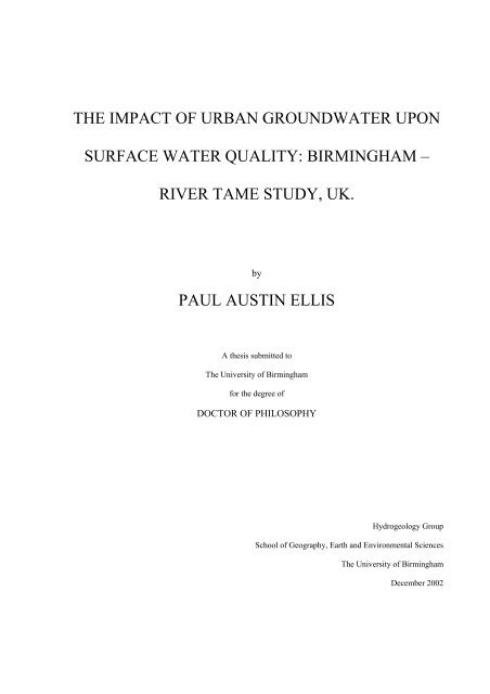
2.1.1 Ground<strong>water</strong> flow to rivers<br />
<strong>The</strong> interaction <strong>of</strong> <strong>ground<strong>water</strong></strong> and <strong>surface</strong> <strong>water</strong> bodies is complex and dependent on many<br />
factors including the topography, geology, climate, and the position <strong>of</strong> the <strong>surface</strong> <strong>water</strong> body<br />
relative to the <strong>ground<strong>water</strong></strong> flow system (Sophocleous, 2002, Winter, 1999 and 2002). Local,<br />
intermediate and/or regional <strong>ground<strong>water</strong></strong> flows may discharge into <strong>surface</strong> <strong>water</strong>s, (Figure<br />
6
REVIEW<br />
2.1) and <strong>surface</strong> <strong>water</strong> may on occasion recharge the <strong>ground<strong>water</strong></strong> (Toth, 1963, Nield et al.,<br />
1994). Hence a reduction in flow or contamination in one will <strong>of</strong>ten affect the other.<br />
Woessner (2000) states that <strong>ground<strong>water</strong></strong> flow to a river channel is dependent on:<br />
1. the distribution and magnitude <strong>of</strong> the hydraulic conductivities within the river channel, the<br />
associated fluvial plain sediments and the underlying bedrock;<br />
2. the relation <strong>of</strong> river stage to the adjacent <strong>ground<strong>water</strong></strong> gradients; and<br />
3. the geometry and position <strong>of</strong> the river channel within the fluvial plain.<br />
Ground<strong>water</strong> is influent to the river channel when the <strong>ground<strong>water</strong></strong> head at the channel<br />
interface is greater than the river stage. Conversely, <strong>surface</strong> <strong>water</strong> is effluent from the channel<br />
when the river stage is higher than the <strong>ground<strong>water</strong></strong> head. Ground<strong>water</strong> through-flow may<br />
occur when the <strong>ground<strong>water</strong></strong> head is higher than the river stage on one bank but lower on the<br />
other (Townley et al., 1992). Ground<strong>water</strong> flow may also occur parallel to the river in which<br />
case only limited <strong>ground<strong>water</strong></strong>/<strong>surface</strong> <strong>water</strong> exchange may occur. During periods <strong>of</strong> high<br />
recharge, <strong>ground<strong>water</strong></strong> ‘mounding’, (ie, rapid increases in head) may occur in the thin<br />
unsaturated zone adjacent to <strong>surface</strong>-<strong>water</strong> bodies which may temporarily influence<br />
<strong>ground<strong>water</strong></strong>/<strong>surface</strong> <strong>water</strong> interactions (Winter, 1983).<br />
A key reference by Winter et al. (1998) summarised the current understanding <strong>of</strong><br />
<strong>ground<strong>water</strong></strong>/<strong>surface</strong> <strong>water</strong> interactions and their relationship to <strong>water</strong> supply, <strong>water</strong> quality<br />
and the aquatic environment, in a variety <strong>of</strong> settings. A unifying framework based on the<br />
concept <strong>of</strong> hydrologic landscapes is used to present conceptual models containing common<br />
7
Abstractions<br />
induce recharge<br />
from <strong>surface</strong><br />
<strong>water</strong>.<br />
Years<br />
River<br />
Days<br />
Flow through<br />
the flood plain<br />
Centuries - Millennia<br />
Ground<strong>water</strong><br />
<strong>surface</strong> <strong>water</strong><br />
exchange<br />
Figure 2.1<br />
Run-<strong>of</strong>f<br />
Ground<strong>water</strong> flow-through Ground<strong>water</strong> influent<br />
Recharge<br />
Aquitard<br />
River gaining River losing<br />
Surface <strong>water</strong> effluent<br />
Figure 2.1 Conceptual model <strong>of</strong> <strong>ground<strong>water</strong></strong> flows to a river
REVIEW<br />
features <strong>of</strong> <strong>ground<strong>water</strong></strong>/<strong>surface</strong> <strong>water</strong> interactions in five general types <strong>of</strong> terrain:<br />
mountainous, riverine, coastal, glacial and dune, and karst.<br />
2.1.2 <strong>The</strong> <strong>ground<strong>water</strong></strong>/<strong>surface</strong> <strong>water</strong> interface<br />
Interactions between <strong>ground<strong>water</strong></strong> and <strong>surface</strong> <strong>water</strong> occur across a transition zone within the<br />
beds <strong>of</strong> lakes, rivers, or seas (Henry, 2002). In the case <strong>of</strong> a river, a ‘hyporheic zone’ develops<br />
where mixing between <strong>ground<strong>water</strong></strong> and <strong>surface</strong> <strong>water</strong> occurs (Biksey et al., 2001). This is an<br />
ecological term that refers to an ecotone where both <strong>ground<strong>water</strong></strong> and <strong>surface</strong> <strong>water</strong> are<br />
present within a stream bed along with a specific set <strong>of</strong> biota (Conant, 2000). <strong>The</strong> flow <strong>of</strong><br />
river <strong>water</strong> over variations in the <strong>surface</strong> <strong>of</strong> the riverbed may cause localised variations in<br />
pressure that induce flow through the riverbed, causing <strong>ground<strong>water</strong></strong>/<strong>surface</strong> <strong>water</strong> mixing<br />
(Figure 2.2). <strong>The</strong> extent <strong>of</strong> this mixing zone may range from centimetres to hundreds <strong>of</strong><br />
meters if <strong>surface</strong> <strong>water</strong> flows through the flood plain sediments are considered (Woessner,<br />
2000, Wroblicky et al., 1998). <strong>The</strong> zone is heterogeneous, dynamic and dependent on the<br />
<strong>surface</strong> <strong>water</strong> and <strong>ground<strong>water</strong></strong> head distribution, river flow, riverbed hydrogeology and<br />
bedform (Fraser et al., 1998).<br />
Large gradients in concentration and environmental conditions <strong>of</strong>ten exist across the transition<br />
zone (Boulton et al., 1998). <strong>The</strong>se affect the spatial and temporal distribution <strong>of</strong> aerobic and<br />
anaerobic microbial processes as well as the chemical form and concentration <strong>of</strong> nutrients,<br />
trace metals and contaminants. Microbial and biological activity may lead to biodegradation<br />
<strong>of</strong> organic contaminants, reducing levels by several orders <strong>of</strong> magnitude within this zone<br />
(Conant, 2000). <strong>The</strong> hyporheic zone is important ecologically because it may store nutrients<br />
(and potentially contaminants), transform compounds biologically and chemically, and<br />
9
(a)<br />
(b)<br />
Ground<strong>water</strong>/<strong>surface</strong> <strong>water</strong><br />
mixing in the hyporheic zone<br />
Ground<strong>water</strong><br />
flow<br />
River Flow<br />
Induced sub<strong>surface</strong><br />
flow <strong>of</strong> river <strong>water</strong><br />
Figure 2.2 Schematic section through a riverbed, (a) longitudinal<br />
(b) lateral (after Winter et al., 1998).<br />
Turbulence<br />
Contaminant plume<br />
with high concentrations<br />
at the core<br />
Riverbed sediments
REVIEW<br />
provide refuge to benthic invertebrates that are the base <strong>of</strong> the aquatic food web (Battin, 1999,<br />
Barnard et al.,1994). Hyporheic organisms are likely to show the effects <strong>of</strong> pollution from<br />
discharging <strong>ground<strong>water</strong></strong> before organisms within the <strong>water</strong> column and so provide an<br />
indicator <strong>of</strong> the <strong>impact</strong> <strong>of</strong> contaminated <strong>ground<strong>water</strong></strong> (Environmental Protection Agency (US),<br />
1998).<br />
Surface <strong>water</strong> exchange and storage within the hyporheic zone influences downstream<br />
nutrient and contaminant transport, and may be associated with enhanced biogeochemical<br />
transformation <strong>of</strong> these compounds in the <strong>surface</strong> <strong>water</strong>. Hyporheic flow paths are typically<br />
small but if rates <strong>of</strong> chemical reactions are rapid enough and the volume <strong>of</strong> exchange great<br />
enough then substantial modifications <strong>of</strong> <strong>surface</strong> <strong>water</strong> quality may occur (Choi et al., 2000,<br />
Packman et al., 2000, Harvey et al., 1993).<br />
2.1.3 Ground<strong>water</strong> contamination<br />
<strong>The</strong> natural background chemistry <strong>of</strong> <strong>ground<strong>water</strong></strong> resulting from recharge composition and<br />
mineral dissolution can be substantially modified by a wide range <strong>of</strong> contaminants that may<br />
be present as different phases within the sub<strong>surface</strong> environment. <strong>The</strong>se include; synthetic<br />
organic compounds, hydrocarbons, metals and other inorganics, and pathogens such as<br />
viruses and bacteria. Conant (2000) summarised the factors that may help to determine the<br />
<strong>impact</strong> <strong>of</strong> a contaminant present in the sub<strong>surface</strong> on a <strong>surface</strong> <strong>water</strong> body. <strong>The</strong>y include:<br />
1. physical and chemical characteristics <strong>of</strong> the contaminants;<br />
2. geometry and temporal variations in the contaminant source;<br />
3. transport mechanisms (advection and dispersion);<br />
4. reactions (reversible and non-reversible).<br />
11
REVIEW<br />
<strong>The</strong> physical and chemical properties <strong>of</strong> the contaminant determine its mobility and toxic<br />
effect. A contaminant may move through the sub<strong>surface</strong> as a pure liquid or gas phase, as a<br />
dissolved phase, in particulate form or attached to colloids. Soluble compounds may be<br />
transported readily within the <strong>ground<strong>water</strong></strong>, and attain high levels <strong>of</strong> concentration. Less<br />
soluble compounds will occur in low concentrations but may provide a long-term source <strong>of</strong><br />
contamination. Advective transport <strong>of</strong> dissolved phase contaminants within the <strong>ground<strong>water</strong></strong><br />
is seen as the primary mechanism by which sub<strong>surface</strong> contaminants may <strong>impact</strong> <strong>upon</strong><br />
<strong>surface</strong> <strong>water</strong> systems.<br />
<strong>The</strong> sources <strong>of</strong> contaminated <strong>ground<strong>water</strong></strong> may be spatially restricted point sources such as an<br />
industrial spill or waste dump, or more diffuse sources such as arise from the widespread<br />
application <strong>of</strong> agricultural fertilisers and pesticides. Point sources tend to give rise to narrow<br />
plumes (Rivett et al., 2001) which migrate with the <strong>ground<strong>water</strong></strong> flow and may eventually<br />
discharge to the <strong>surface</strong> <strong>water</strong> (Figure 2.3). In the USA more than 75% <strong>of</strong> the contaminated<br />
land categorised under the government’s ‘superfund’ sites lie within 0.5 miles <strong>of</strong> a <strong>surface</strong><br />
<strong>water</strong> body and more than half had an <strong>impact</strong> on <strong>surface</strong> <strong>water</strong> in some way (Environmental<br />
Protection Agency (U.S.), 2000).<br />
<strong>The</strong> initial contaminant concentration in the <strong>ground<strong>water</strong></strong> will depend on the mass and<br />
distribution <strong>of</strong> the contaminant in the source area, the rate <strong>of</strong> <strong>ground<strong>water</strong></strong> flow and the<br />
physical-chemical-biological processes controlling contaminant dissolution (Fetter, 1999).<br />
Contaminants derived from the land <strong>surface</strong> may take a considerable time to enter the<br />
<strong>ground<strong>water</strong></strong> if a large unsaturated zone is present. Ground<strong>water</strong> contaminant concentrations<br />
in the source area may vary with time or may give rise to discrete pulse-type inputs.<br />
12
Abstraction<br />
For<br />
drinking<br />
<strong>water</strong><br />
supply<br />
Seepage<br />
face<br />
Hyporheic<br />
zone<br />
Contaminated<br />
tributaries<br />
Surface<br />
<strong>water</strong><br />
exchange<br />
Sediment<br />
grains<br />
Eh.<br />
PH<br />
Temperature<br />
Concentration<br />
Gradients<br />
Diffuse <strong>urban</strong><br />
and agricultural<br />
pollution<br />
Pipe end discharge<br />
Capillary<br />
fringe<br />
Dilution and<br />
dispersion<br />
Leaking<br />
sewers<br />
Converging<br />
<strong>ground<strong>water</strong></strong> flows<br />
Point source<br />
Contaminant plume<br />
Leachate<br />
from<br />
contaminated<br />
land<br />
Natural<br />
mineral<br />
dissolution<br />
Dissolved phase<br />
PROCESSES IN THE RIVERBED<br />
Ground<strong>water</strong> / <strong>surface</strong> <strong>water</strong> mixing<br />
Interstitial transport <strong>of</strong> particulates / colloids<br />
Precipitation / dissolution reaction<br />
Sorption and ion exchange<br />
Line source<br />
LNAPL<br />
Bacterial activity may;<br />
consume nutrients and oxygen, mediate redox<br />
reactions biodegrade organic contaminants<br />
Benthic fauna may be affected by contaminants<br />
Figure 2.3 Conceptual model <strong>of</strong> contaminant inputs to a river.<br />
Recharge<br />
+<br />
aerial<br />
contaminant<br />
deposition<br />
Industrial<br />
spills<br />
DNAPL
REVIEW<br />
Contaminant concentrations within the <strong>ground<strong>water</strong></strong> will be modified en route to, and across,<br />
the <strong>ground<strong>water</strong></strong>/<strong>surface</strong> <strong>water</strong> interface. Dispersion will result in spreading and mixing <strong>of</strong> the<br />
contaminant plume with cleaner <strong>ground<strong>water</strong></strong>. However, lateral dispersion within an aquifer is<br />
generally low and the plume remains narrow relative to its length, the highest contaminant<br />
concentrations being within the central core (Rivett et al., 2001). When the plume reaches the<br />
hyporheic zone, more turbulent conditions are likely to exist as the <strong>ground<strong>water</strong></strong> mixes with<br />
the <strong>surface</strong> <strong>water</strong> and is ultimately diluted in the <strong>surface</strong>-<strong>water</strong> column.<br />
During transport, the contaminants may undergo reversible reactions such as adsorption,<br />
precipitation/dissolution and ion exchange, and non-reversible reactions such as<br />
biodegradation. Reactions may be reversible only under certain conditions. For example<br />
desorption <strong>of</strong> heavy metals occurs under conditions <strong>of</strong> low pH, and therefore contaminants<br />
may be effectively removed from the system until conditions change. <strong>The</strong> types <strong>of</strong> reactions<br />
that occur are dependent on the local conditions, and these may vary considerably along the<br />
contaminant flow path from the source area, through the aquifer to the <strong>ground<strong>water</strong></strong>/<strong>surface</strong><br />
<strong>water</strong> interface. <strong>The</strong>re are key processes controlling the movement and transport <strong>of</strong><br />
contaminants across the <strong>ground<strong>water</strong></strong>/<strong>surface</strong> <strong>water</strong> interface.<br />
1. Bacterial action which may play an important role in catalysing reactions (e.g. sulphate<br />
and nitrate reduction) and directly degrading some organic compounds. <strong>The</strong><br />
<strong>ground<strong>water</strong></strong>/<strong>surface</strong> <strong>water</strong> interface <strong>of</strong>ten has a high nutrient content and anoxic<br />
conditions which are conducive to bacterial action.<br />
2. Adsorption <strong>of</strong> contaminants to sites on the surrounding aquifer material. This reaction is<br />
generally reversible in which case it will not alter the total mass flux <strong>of</strong> the contaminants<br />
but it may significantly retard their transport allowing extra time for other processes to<br />
14
REVIEW<br />
occur such as biodegradation. For organic contaminants, the degree <strong>of</strong> sorption is <strong>of</strong>ten<br />
proportional to the content <strong>of</strong> organic carbon which is generally much higher in the<br />
riverbed sediments relative to the surrounding geology (Schwarzenbach et al., 1981). For<br />
inorganic contaminants, clay minerals, organic matter and oxides/hydroxides all have a<br />
sorption and exchange capacity which may retard contaminant transport (Appelo and<br />
Postma, 1999).<br />
3. Rapid changes in pH, Eh, and mixing <strong>of</strong> <strong>water</strong>s <strong>of</strong> significantly differing concentrations<br />
occur across the <strong>ground<strong>water</strong></strong>/<strong>surface</strong> <strong>water</strong> interface. Ground<strong>water</strong> chemistry which may<br />
have been in equilibrium will adjust rapidly to the new conditions, perhaps leading to<br />
sudden mineral precipitation. Iron oxides are a common example <strong>of</strong> precipitation occuring<br />
when acidic, oxygen-poor <strong>ground<strong>water</strong></strong> mixes with higher pH, more highly oxygenated<br />
<strong>surface</strong> <strong>water</strong>s.<br />
Contaminant movement and transformation across the <strong>ground<strong>water</strong></strong>/<strong>surface</strong> <strong>water</strong> interface<br />
are poorly understood. In light <strong>of</strong> this a workshop was held to summarise the existing<br />
knowledge base on the <strong>ground<strong>water</strong></strong>/<strong>surface</strong> <strong>water</strong> interface and to develop strategies for an<br />
improved understanding <strong>of</strong> the effect <strong>of</strong> contaminated <strong>ground<strong>water</strong></strong> discharge through it. <strong>The</strong><br />
proceedings <strong>of</strong> this workshop provide a key reference on this subject area (Environmental<br />
Protection Agency (U.S.), 2000).<br />
It is predicted that by 2010, half the world’s population <strong>of</strong> 6,500 million will live in towns or<br />
cities, and that much <strong>of</strong> the <strong>urban</strong> growth will be in developing countries (Morris, 2002).<br />
Increasing demand will be placed on both <strong>urban</strong> <strong>ground<strong>water</strong></strong> and <strong>surface</strong> <strong>water</strong> resources for<br />
domestic and industrial use. Unfortunately, <strong>urban</strong> growth is <strong>of</strong>ten associated with degradation<br />
15
REVIEW<br />
<strong>of</strong> <strong>water</strong> quality which limits the usefulness <strong>of</strong> both <strong>ground<strong>water</strong></strong> and <strong>surface</strong> <strong>water</strong> resources<br />
(Petts et al., 2002). <strong>The</strong> occurrence <strong>of</strong> contaminated <strong>ground<strong>water</strong></strong> related to <strong>urban</strong>isation is<br />
well known, both in the U.K. (Barrett et al., 1997, Lerner et al., 1996, Ford et al., 1994, Rivett<br />
et al., 1990) and abroad (Eiswirth et al., 1997, Kacaroglu et al., 1997, Appleyard, 1995).<br />
Likewise, the occurrence <strong>of</strong> poor quality <strong>urban</strong> <strong>surface</strong> <strong>water</strong>s is extremely common<br />
(Kayabalý et al., 1999, Ziegler et al., 2001). However, <strong>urban</strong> <strong>ground<strong>water</strong></strong> and <strong>surface</strong> <strong>water</strong><br />
interactions are less well understood.<br />
2.2 International Case Studies<br />
To characterise the <strong>impact</strong> <strong>of</strong> <strong>urban</strong> <strong>ground<strong>water</strong></strong> on <strong>surface</strong>-<strong>water</strong> quality requires a broad<br />
multidisciplinary approach involving hydrological, hydrogeological, hydrochemical and<br />
ecological elements. To cover all these elements is generally beyond the scope <strong>of</strong> a single<br />
study and previous work has <strong>of</strong>ten focussed on a particular <strong>ground<strong>water</strong></strong> and/or <strong>surface</strong> <strong>water</strong><br />
flow and/or quality issue. <strong>The</strong> scale <strong>of</strong> the studies can be divided into those that provide<br />
detailed but localised information on a specific contaminant plume or process across the river<br />
bed, and those that provide more general regional information on <strong>surface</strong>-<strong>water</strong> quality and<br />
flow. Only limited work has been done on scaling up the effects <strong>of</strong> local processes to the<br />
catchment scale. <strong>The</strong> <strong>urban</strong> <strong>ground<strong>water</strong></strong> system generally lies between these two extremes <strong>of</strong><br />
scale, having many potential contaminant sources but covering a limited extent <strong>of</strong> the total<br />
catchment area.<br />
16
2.2.1 Water quality studies<br />
REVIEW<br />
Relationships between <strong>ground<strong>water</strong></strong> and <strong>surface</strong>-<strong>water</strong> quality have been investigated for<br />
nutrients, pesticides , volatile organic compounds and metals (Lindsey et al., 1998, Bevans et<br />
al., 1998). A major study <strong>of</strong> the <strong>surface</strong> <strong>water</strong> and <strong>ground<strong>water</strong></strong> quality in the Potomac River<br />
Basin, USA, revealed a substantial <strong>impact</strong> from anthropogenic sources <strong>of</strong> contamination<br />
related to <strong>urban</strong>isation (Ator et al., 1998). Chlorodane, DDT, PCBs, mercury and lead were all<br />
detected in streambed sediment and aquatic tissues derived from persistent sources, such as<br />
<strong>ground<strong>water</strong></strong>, within the river basin. Grischek et al. (1996) investigated <strong>urban</strong> <strong>ground<strong>water</strong></strong><br />
quality beneath the city <strong>of</strong> Dresden in Germany and found the influent <strong>surface</strong> <strong>water</strong> from the<br />
River Elbe to have only a limited effect. Hartwell (1997) investigated the transport <strong>of</strong> the<br />
herbicide atrazine between the Cedar River and <strong>ground<strong>water</strong></strong> in Iowa, USA. <strong>The</strong> study found<br />
that <strong>ground<strong>water</strong></strong> from the adjacent alluvial aquifer was the principal source <strong>of</strong> atrazine in the<br />
river during base-flow conditions.<br />
Lorah et al. (1999) and Conant (2000) investigated the discharge <strong>of</strong> chlorinated solvent<br />
plumes to <strong>surface</strong> <strong>water</strong> systems and found evidence for enhanced biodegradation across the<br />
interface. Schwarzenbach et al. (1981) conducted some <strong>of</strong> the earliest work on<br />
<strong>ground<strong>water</strong></strong>/<strong>surface</strong> <strong>water</strong> contaminant interactions based on laboratory simulations <strong>of</strong> field<br />
conditions beneath a river valley in Switzerland. <strong>The</strong>y conducted a ‘classic’ set <strong>of</strong> sorption<br />
studies and showed sorption to organic carbon to be a key process in retarding the transport <strong>of</strong><br />
non-polar organic compounds across the <strong>ground<strong>water</strong></strong>/<strong>surface</strong> <strong>water</strong> interface.<br />
Metal contamination resulting from acidic <strong>ground<strong>water</strong></strong> associated with mining activities has<br />
been widely researched (Benner et al., 1995, Kimball et al., 2002). Paulson (1997)<br />
17
REVIEW<br />
investigated the transport and fate <strong>of</strong> Fe, Mn, Cu, Zn, Cd, Pb and SO4 in a <strong>ground<strong>water</strong></strong> plume<br />
and in the downstream <strong>surface</strong> <strong>water</strong>s in the Coeur d’Alene Mining District in the US. He<br />
found that <strong>upon</strong> mixing with higher pH <strong>surface</strong> <strong>water</strong> the metals were lost from solution in the<br />
following order: Fe>Al>Pb>Cu>Mn>Zn> Cd. Less than 10% <strong>of</strong> the dissolved Zn and Cd<br />
were lost, despite a 5 km journey through both the <strong>ground<strong>water</strong></strong> and <strong>surface</strong> <strong>water</strong> regimes.<br />
Paulson and Balistrieri (1999) used model simulations and laboratory experiments to examine<br />
the removal <strong>of</strong> Cd, Cu, Pb and Zn in acidic <strong>ground<strong>water</strong></strong> during neutralisation by ambient<br />
<strong>surface</strong> <strong>water</strong>s. <strong>The</strong>y concluded that hydrous Fe oxides and particulate organic carbon are<br />
more important than hydrous Al oxides in removing metals from the <strong>ground<strong>water</strong></strong>. Tessier et<br />
al. (1996) found that trace metals present in <strong>water</strong> influent to two lakes in Canada sorbed<br />
directly to the OH functional groups <strong>of</strong> iron and manganese oxyhroxides and organic matter<br />
found in the lake sediments. Kuwabara et al. (1999) found that <strong>water</strong> flowing through the bed<br />
<strong>of</strong> lake Coeur d’Alene caused a significant flux <strong>of</strong> metal from the lake sediments to the <strong>water</strong><br />
column.<br />
2.2.2 Flow Studies<br />
<strong>The</strong> <strong>ground<strong>water</strong></strong> support <strong>of</strong> river baseflow and its relationship to the underlying geology has<br />
has long been recognised and studied (Meyboom, 1961, Mau et al., 1993, Pinder et al., 1969,<br />
O’Conner 1976,). Several studies have investigated the relationship between reduced <strong>surface</strong><br />
<strong>water</strong> flows and increased levels <strong>of</strong> <strong>ground<strong>water</strong></strong> abstraction (Sophocleous 2000). A<br />
comprehensive study on the interaction <strong>of</strong> the Equus Beds alluvial aquifer and the Arkansas<br />
River, USA, found that abstraction for irrigation significantly reduced river baseflow levels<br />
and induced <strong>surface</strong> <strong>water</strong> seepage into the aquifer (Ziegler et al., 2001). <strong>The</strong> response <strong>of</strong><br />
<strong>ground<strong>water</strong></strong> to transient <strong>surface</strong> <strong>water</strong> levels has been used to derive estimates <strong>of</strong> the aquifer<br />
property S/T (Reynolds, 1987, Workman et al., 1997, Erskine 1991). Devito et al. (1996)<br />
18
REVIEW<br />
investigated <strong>ground<strong>water</strong></strong>/<strong>surface</strong> <strong>water</strong> interactions and the <strong>ground<strong>water</strong></strong> contribution to<br />
wetlands on the Canadian Shield and demonstrated the control <strong>of</strong> morphology and shallow<br />
sub<strong>surface</strong> geology on the hydrology <strong>of</strong> valley bottom swamps. Wroblicky et al. (1998)<br />
investigated the <strong>ground<strong>water</strong></strong> flow and seasonal variations in the hyporheic zone for two first<br />
order mountain streams in the US. <strong>The</strong> streams were in alluvial material with different<br />
hydraulic properties derived from bedrock types comprising welded tuff and sandstone.<br />
Numerical modelling was used to simulate unconfined transient flow. Sensitivity analyses<br />
indicated that changes in the hydraulic conductivity <strong>of</strong> the alluvial and streambed sediments<br />
and variation in recharge rates have greatest <strong>impact</strong> on the magnitude, direction, and spatial<br />
distribution <strong>of</strong> stream/<strong>ground<strong>water</strong></strong> exchange.<br />
2.2.3 Combined Quality and Flow Studies<br />
Case studies <strong>of</strong> <strong>ground<strong>water</strong></strong>/<strong>surface</strong> <strong>water</strong> quality and flow interactions have generally been<br />
conducted in a rural setting (Cey et al., 1998, Pionke et al., 1998) in order to avoid the<br />
complexities associated with <strong>urban</strong> rivers which have many inputs (Ellis et al., 2002,<br />
Appendix 1). Gburek et al. (1999) investigated the flow and major ion contributions to<br />
baseflow in an upland <strong>water</strong>shed in Canada. <strong>The</strong> study showed increased ionic concentrations,<br />
including nitrate, within <strong>ground<strong>water</strong></strong> baseflow derived from an area <strong>of</strong> agricultural land<br />
compared with low ionic concentrations from forested areas. A chemical mass balance (i.e<br />
concentration x flow) was used to investigate the contribution <strong>of</strong> <strong>ground<strong>water</strong></strong> from different<br />
parts <strong>of</strong> the study area. A simple model was developed based on land use to explain nitrate<br />
concentrations within baseflow.<br />
Diffuse nitrate pollution <strong>of</strong> <strong>surface</strong> <strong>water</strong>s from <strong>ground<strong>water</strong></strong> has been investigated in several<br />
studies in the USA (MacNish et al., 1998). (Bachman et al., 1997) used river baseflow<br />
analyses and <strong>surface</strong> <strong>water</strong> quality sampling to calculate nitrate loading to Chesapeake Bay.<br />
19
REVIEW<br />
<strong>The</strong> median <strong>ground<strong>water</strong></strong> contribution was estimated as 56% <strong>of</strong> the total nitrate load under<br />
baseflow. Harvey et al. (1998) examined the effect <strong>of</strong> enhanced maganese oxidation (and co-<br />
precipitation <strong>of</strong> trace metals) in the hyporheic zone on basin-scale geochemical mass balance<br />
in a drainage basin contaminated by copper mining.<br />
2.3 UK Case Studies<br />
Published data on <strong>ground<strong>water</strong></strong> quality and flow interactions in the UK are generally limited.<br />
A few <strong>of</strong> the key studies are briefly presented.<br />
A study <strong>of</strong> trace-element concentrations in the major rivers entering the Humber estuary<br />
showed elevated levels in the rivers draining industrial <strong>urban</strong> catchments (Neal et al., 1996).<br />
<strong>The</strong> relationship between concentration and flow was used to evaluate the sources <strong>of</strong> trace<br />
elements; a negative relationship to flow implied a <strong>ground<strong>water</strong></strong> source. Within the <strong>urban</strong><br />
rivers, most elements in the dissolved phase exhibited negative relationships, indicating that<br />
point-source discharges provided the major source <strong>of</strong> trace elements. Roberts et al. (1998)<br />
investigated nitrate contamination <strong>of</strong> <strong>ground<strong>water</strong></strong> in the Lincolnshire Limestone resulting<br />
from <strong>surface</strong> <strong>water</strong> recharge related to local <strong>ground<strong>water</strong></strong> abstractions.<br />
Of particular concern in the UK has been the widespread detection <strong>of</strong> pesticides at low levels<br />
within <strong>ground<strong>water</strong></strong>s and <strong>surface</strong> <strong>water</strong>s (Croll, 1991). Clark et al. (1991) investigated<br />
pesticide occurrence in the River Granta and the underlying <strong>ground<strong>water</strong></strong> within the chalk<br />
aquifer <strong>of</strong> Cambridgeshire. <strong>The</strong> maximum levels <strong>of</strong> pesticide were found in the river during<br />
periods <strong>of</strong> high flow. However, even under low-flow conditions, levels <strong>of</strong> pesticide were<br />
persistent and are probably derived from the <strong>ground<strong>water</strong></strong>. Of particular interest in the study,<br />
20
REVIEW<br />
owing to their widespread detection and/or application, were the pesticides atrazine, simazine,<br />
isoproturon, chlortoluron and tri-allate.<br />
Hooda et al. (1997) found the <strong>impact</strong> <strong>of</strong> diffuse phosphorous loading on six small catchments<br />
in Scotland to be greatest during summer <strong>ground<strong>water</strong></strong>-fed baseflow conditions. Birtles,<br />
(1978) modelled <strong>water</strong> quality in the River Severn by separating the river hydrographs into<br />
discrete components each <strong>of</strong> which had separate, conservative, <strong>surface</strong> <strong>water</strong> quality<br />
parameters. <strong>The</strong>se comprised, direct run-<strong>of</strong>f, baseflow from the Triassic Sandstone deposits,<br />
baseflow from superficial deposits and effluent returns. Younger et al. (1993) investigated<br />
<strong>ground<strong>water</strong></strong>/<strong>surface</strong> <strong>water</strong> interactions in the Thames basin.<br />
Research currently in progress in the UK is summarised by Young et al. (2002). New research<br />
initiatives are under way to provide support for integrated <strong>ground<strong>water</strong></strong>/<strong>surface</strong> <strong>water</strong><br />
monitoring and assessment for sustainable catchment management. <strong>The</strong>se include the<br />
Lowland Catchment Research Programme, LOCAR, (Peach et al., 2000, LOCAR, 2002) and<br />
the Catchment Hydrology and Sustainable Management (CHASM) group which will<br />
investigate highland catchments (CHASM, 2002). <strong>The</strong> recently concluded Land-Ocean<br />
Interaction Study (LOIS, 1998) was undertaken to quantify the chemical fluxes entering the<br />
North Sea from the surrounding countries, including the UK. Extensive data sets were<br />
collected for the Humber catchment which incorporate the <strong>ground<strong>water</strong></strong> contribution to the<br />
total geochemical flux to the sea. Most <strong>of</strong> the current research is focussed on rural catchments<br />
and there is a lack <strong>of</strong> ongoing research into <strong>urban</strong> <strong>ground<strong>water</strong></strong>/<strong>surface</strong> <strong>water</strong> interactions.<br />
21
2.3.1 UK Legislation<br />
REVIEW<br />
<strong>The</strong> new Water Framework Directive (Council <strong>of</strong> Europe, 2000, Environment Agency, 2002)<br />
has been introduced to ensure an integrated approach to the management <strong>of</strong> catchment <strong>surface</strong><br />
and <strong>ground<strong>water</strong></strong> quality and flow. Consultations are under way in the UK on the<br />
implementation <strong>of</strong> this directive (DEFRA, 2002). It will be implemented in conjunction with<br />
other legislation such as Part IIa <strong>of</strong> the Environmental Protection Act 1990 designed to<br />
maintain and improve the quality <strong>of</strong> <strong>surface</strong> and <strong>ground<strong>water</strong></strong>. Under the legislation, the<br />
<strong>impact</strong> <strong>of</strong> land causing pollution <strong>of</strong> controlled <strong>water</strong>s must be assessed by comparison to the<br />
background <strong>water</strong> quality and suitable standards such as drinking <strong>water</strong> and environmental<br />
quality standards (EQS) for <strong>surface</strong> <strong>water</strong>s (Smith, 2002). Contaminated land and<br />
contaminated <strong>ground<strong>water</strong></strong>s arising, where found to cause significant <strong>impact</strong>s on the <strong>surface</strong><br />
<strong>water</strong> are likely to require remedial action (Rivett et al., 2002).<br />
2.4 Monitoring methods<br />
Comprehensive reviews <strong>of</strong> the existing analytical, numerical, field and chemical investigative<br />
techniques for <strong>ground<strong>water</strong></strong>/<strong>surface</strong> <strong>water</strong> interactions have been carried out by HRU (2001)<br />
and Winter (1995). On the catchment scale, the most widely-used approach is river<br />
hydrograph separation and baseflow recession analyses to derive the <strong>ground<strong>water</strong></strong> component<br />
<strong>of</strong> river flow (Meyboom, 1961, Mau et al., 1997, Gustard et al., 1992). Several workers<br />
(Pinder et al., 1969, O’Conner 1976, Birtles 1978) have used differences in <strong>ground<strong>water</strong></strong> and<br />
<strong>surface</strong> <strong>water</strong> chemistry and total dissolved solids to resolve further the <strong>ground<strong>water</strong></strong><br />
component <strong>of</strong> the river hydrographs. At the smaller scale <strong>of</strong> the river reach, stream tracers<br />
22
REVIEW<br />
have been used to determine river discharge accretion and characterise river sub<strong>surface</strong> <strong>water</strong><br />
exchange (Harvey et al., 1996, Kimball, 2002).<br />
Piezometers and piezometer nests have been used in several studies to obtain <strong>water</strong> samples<br />
and head measurements within the <strong>ground<strong>water</strong></strong>/<strong>surface</strong> <strong>water</strong> interface (Dean et al., 1999,<br />
Cey et al., 1998, Lee, 1980, Henry, 2000). Other in situ sampling devices have also been<br />
developed such as the colonisation corer (Fraser et al., 1996) and the bead tube sampler<br />
(Moore, 2000). Passive sampling techniques based on diffusive gradients across semi-<br />
permeable membrane devices have been used to detect both hydrophobic organics and heavy<br />
metals in aquatic environments (Vroblesky et al., 1997; Church et al., 2000). A number <strong>of</strong><br />
devices have been developed to measure the seepage across a lake or riverbed (Lee, 1977;<br />
Carr et al., 1980; Isiorho, 1999) although the methods <strong>of</strong>ten encounter errors when used in<br />
fast-flowing river environments (Libelo et al., 1994). <strong>The</strong> temperature gradient across the<br />
<strong>ground<strong>water</strong></strong>/<strong>surface</strong> <strong>water</strong> interface has been used to determine flow rates (Silliman et al.,<br />
1995, Evans et al. 1997). Several <strong>of</strong> the investigative methods identified in the literature<br />
review were adapted for use in the present study.<br />
2.5 Modelling methods<br />
A review <strong>of</strong> analytical and numerical methods <strong>of</strong> modelling river-aquifer interactions are<br />
presented by HRU (2001), Winter (1995) and Younger (1989). Analytical solutions have been<br />
developed from early simulations <strong>of</strong> 1D <strong>ground<strong>water</strong></strong> interaction with fully penetrating<br />
streams (Rorabaugh, 1964) to meet a range <strong>of</strong> applications. <strong>The</strong>se include the simulation <strong>of</strong><br />
bank storage and <strong>ground<strong>water</strong></strong> fluctuations during river flood events (Serrano and Workman,<br />
23
REVIEW<br />
1998, Reynolds, 1987, Hunt, 1990), travel times for <strong>surface</strong> <strong>water</strong> into contiguous aquifers<br />
(Heij, 1989) and the effects <strong>of</strong> pumping <strong>ground<strong>water</strong></strong> on stream flow (Spalding et al., 1991).<br />
<strong>The</strong> onset <strong>of</strong> readily available computing power has led to an increase in the use <strong>of</strong> numerical<br />
models to simulate <strong>ground<strong>water</strong></strong>/<strong>surface</strong> <strong>water</strong> interactions. <strong>The</strong>se have been successfully<br />
applied to numerous field studies for different hydrogeologic settings and scales (Modica,<br />
1993, Jorgensen et al., 1989, Younger, 1989, Rushton et al., 1989, Sophocleous, 1991). Most<br />
models use idealised stream geometry and the Darcy equation to simulate transfer <strong>of</strong> <strong>water</strong><br />
across the streambed sediments. In this case <strong>ground<strong>water</strong></strong> discharge = hydraulic conductivity<br />
x hydraulic gradient x cross sectional area. This may <strong>of</strong>ten be an oversimplification <strong>of</strong> the<br />
natural system. Previous workers (Rushton et al., 1979) indicate that the relationship between<br />
discharge and hydraulic gradient is not always linear, with variations occurring in the<br />
hydraulic conductivity, particularly if flow reversal occurs. Near <strong>surface</strong> <strong>water</strong> bodies,<br />
convergent flow with a considerable vertical component <strong>of</strong>ten occurs which must be<br />
accounted for if hydraulic conductivity is anisotropic.<br />
<strong>The</strong> realistic simulation <strong>of</strong> transient <strong>surface</strong> <strong>water</strong> flows and <strong>ground<strong>water</strong></strong> flows across a<br />
region is complex. Surface <strong>water</strong> and <strong>ground<strong>water</strong></strong> flow equations may be coupled and solved<br />
simultaneously by iteration. However, more commonly the <strong>surface</strong> <strong>water</strong> heads are set (from<br />
field data or separate modelling) or river baseflow is determined as output from a<br />
<strong>ground<strong>water</strong></strong> model (Younger, 1989). <strong>The</strong> widely used <strong>ground<strong>water</strong></strong> flow model MODFLOW<br />
(Macdonald and Harbaugh, 1988) has been adapted to incorporate a 1D simulation <strong>of</strong><br />
unsteady flow in open-channel networks, but still utilises the simple Darcy equation for <strong>water</strong><br />
transfer. Other models have been developed to investigate <strong>ground<strong>water</strong></strong>/<strong>surface</strong> <strong>water</strong><br />
interaction for variably saturated <strong>ground<strong>water</strong></strong> systems for losing streams (Riesenauer, 1963)<br />
24
REVIEW<br />
and under conditions <strong>of</strong> non-uniform recharge adjacent to a <strong>surface</strong> <strong>water</strong> body (Winter, 1983,<br />
Cooley 1983). Models have been used to evaluate the effect <strong>of</strong> <strong>ground<strong>water</strong></strong> pumping on<br />
stream flow for <strong>water</strong> resources and environmental <strong>impact</strong> purposes (Sophocleous, 2000,<br />
Eberts and Blair, 1990). Flow and transport modelling has been used to investigate solute<br />
(contaminant) transfer between <strong>ground<strong>water</strong></strong> and <strong>surface</strong> <strong>water</strong> on the regional scale (Duffy<br />
and Lee, 1992, Jakeman et al., 1989). Geochemical models such as the USGS model<br />
PHREEQC have been used to simulate solute fate and transport across the<br />
<strong>ground<strong>water</strong></strong>/<strong>surface</strong> <strong>water</strong> interface (Van Breukelen et al., 1998).<br />
2.6 Conclusions<br />
Ground<strong>water</strong>/<strong>surface</strong> <strong>water</strong> quality and flow interactions are complex and variable between<br />
and within catchments. Further work is required to better understand the link between quality<br />
and flow processes, particularly in an <strong>urban</strong> setting where research to date has been limited.<br />
<strong>The</strong> <strong>ground<strong>water</strong></strong>/<strong>surface</strong> <strong>water</strong> interface is ecologically important and is a major pathway for<br />
mass transfer between the sub<strong>surface</strong> and <strong>surface</strong>. Contaminant and nutrient concentrations<br />
within both the <strong>ground<strong>water</strong></strong> and <strong>surface</strong> <strong>water</strong> may be altered significantly during their<br />
passage through the <strong>ground<strong>water</strong></strong>/<strong>surface</strong> <strong>water</strong> interface. <strong>The</strong> interface <strong>of</strong>ten shows high<br />
environmental and concentration gradients. Significant processes that occur across this zone<br />
that may affect contaminant fate and transport include; sorption and precipitation reactions<br />
and bacterial activity which may mediate chemical reactions and degrade organic<br />
contaminants. <strong>The</strong> key references identified in the review <strong>of</strong> <strong>ground<strong>water</strong></strong>-<strong>surface</strong> interactions<br />
were, Sophocleous (2002), Winter et al. (1998), EPA (2000), and Woessner (2000). Useful<br />
case studies <strong>of</strong> <strong>ground<strong>water</strong></strong> quality and flow interactions were Cey et al. (1998) and Gburek<br />
et al. (1999).<br />
25
CHAPTER 3. STUDY SETTING<br />
STUDY SETTING<br />
<strong>The</strong> River Tame drains a 408 km 2 highly <strong>urban</strong>ised catchment covering part <strong>of</strong> the West<br />
Midlands conurbation, which currently supports a population in excess <strong>of</strong> 1.8 million, and<br />
includes Birmingham the UK’s second largest city. <strong>The</strong> Tame forms part <strong>of</strong> the larger<br />
drainage system <strong>of</strong> the River Trent, which eventually drains to the North Sea. It rises to the<br />
east <strong>of</strong> a ridge that forms part <strong>of</strong> the major <strong>water</strong>shed <strong>of</strong> central England with the River Stour<br />
in the Severn catchment to the west draining to the Bristol Channel. <strong>The</strong> three upper arms <strong>of</strong><br />
the Tame (Figure 3.1) rise in the ‘Black Country’ towns <strong>of</strong> Wolverhampton, Walsall and<br />
Oldbury before joining to flow eastwards through the northern part <strong>of</strong> Birmingham. <strong>The</strong> river<br />
baseflow is supported by contributions from sewage effluent and other industrial discharges<br />
plus a significant contribution from <strong>ground<strong>water</strong></strong> which may increase the flow by >20%<br />
across the research area. <strong>The</strong> 24 km study reach lies between the gauging stations <strong>of</strong> Bescot<br />
and Water Orton and work has been focused on the central 7.4 km section that overlies the<br />
unconfined Birmingham Aquifer.<br />
3.1 Historical Background<br />
<strong>The</strong> West Midlands conurbation has been a population centre for the past 200 years and a<br />
major centre for heavy industry since the industrial revolution. Rapid development <strong>of</strong> the area<br />
occurred during the industrial revolution based on the exploitation and processing <strong>of</strong> raw<br />
materials from the South Staffordshire Coal Field and local ironstone deposits. A series <strong>of</strong><br />
canals (from 1800) and later railways (from 1840) were constructed connecting various<br />
26
(b)<br />
(a)<br />
River Tame<br />
10 m<br />
topographic<br />
contours<br />
Motorway<br />
Railway<br />
Regional<br />
Study Reach<br />
Detailed<br />
Study Reach<br />
Figure 3.1 (a) Catchment map <strong>of</strong> the Upper Tame (b) Topography <strong>of</strong> the detailed study<br />
reach (c) Regional Setting<br />
(c)
STUDY SETTING<br />
sections <strong>of</strong> the city with the rest <strong>of</strong> the country and facilitating the rapid growth and spread <strong>of</strong><br />
<strong>urban</strong>isation. <strong>The</strong> sparsely populated semi-rural area was transformed into a series <strong>of</strong><br />
gradually expanding towns that have eventually coalesced to form the West Midlands<br />
conurbation. <strong>The</strong> region became a major centre for metal working and manufacturing<br />
industries with productivity reaching maximum levels during the two world wars. Because <strong>of</strong><br />
this development, a large demand was placed on both <strong>surface</strong> <strong>water</strong> and <strong>ground<strong>water</strong></strong><br />
resources for industrial and public supply.<br />
Contamination <strong>of</strong> soils, <strong>ground<strong>water</strong></strong> and <strong>surface</strong> <strong>water</strong> occurred as a result <strong>of</strong> the <strong>urban</strong>isation<br />
with little or no legislation in place to control it. This pollution combined with sewage<br />
effluent and industrial discharges began to seriously effect river quality during the 19 th<br />
Century. By 1870 Birmingham City had major problems with the disposal <strong>of</strong> sewage effluent<br />
and the continued deterioration <strong>of</strong> <strong>water</strong> quality in the Tame prompted the construction <strong>of</strong> the<br />
Elan Valley reservoirs in Mid Wales to achieve an adequate public supply. This had the effect<br />
<strong>of</strong> increasing flow in the Tame which received the increased levels <strong>of</strong> sewage effluent.<br />
Because <strong>of</strong> overloading <strong>of</strong> the sewerage system untreated effluents <strong>of</strong>ten entered the river and<br />
by 1918 the Tame supported no fish life and by 1945 virtually no aquatic life (Clay, 2000).<br />
Today, the Tame, which once supported salmon and trout has no sustainable fish population<br />
in the study area (Crabtree et al., 1998). Ground<strong>water</strong> quality in the Birmingham Aquifer also<br />
showed a substantial deterioration with many public supply wells polluted and abandoned by<br />
1920 (Greswell et al., 2000).<br />
Since the 1950s’ modification <strong>of</strong> the sewerage system, a reduction in heavy industry and the<br />
implementation <strong>of</strong> better pollution control has helped to improve the <strong>surface</strong> <strong>water</strong> quality.<br />
28
STUDY SETTING<br />
But under the General Quality Assessment (Environment Agency, 1998) the Tame is still<br />
categorised within the worst classes E/F (poor/bad) with severe <strong>impact</strong>s reported on the river<br />
ecology. Rapid <strong>urban</strong> run-<strong>of</strong>f from precipitation events can generate high <strong>surface</strong> <strong>water</strong> flows<br />
and large pollutant loads that add to the hostile conditions for aquatic life.<br />
<strong>The</strong> long history <strong>of</strong> industrialisation and <strong>urban</strong>isation has left a legacy <strong>of</strong> contaminated land,<br />
which has caused significant inorganic and more recently organic contamination <strong>of</strong> the<br />
underlying <strong>ground<strong>water</strong></strong>. <strong>The</strong> contribution <strong>of</strong> sewage effluent and industrial pipe end<br />
discharges to the <strong>surface</strong> <strong>water</strong> quality and flow are relatively well understood but little is<br />
known about the contribution <strong>of</strong> <strong>ground<strong>water</strong></strong> across the study reach.<br />
3.2 Land use<br />
Heavy industry and housing grew up side by side with little or no legislation to control<br />
contamination <strong>of</strong> soils, <strong>ground<strong>water</strong></strong> and <strong>surface</strong> <strong>water</strong>.<br />
Studies <strong>of</strong> <strong>urban</strong> <strong>ground<strong>water</strong></strong> pollution throughout the UK (Lerner et al.,1996) and in nearby<br />
Wolverhampton (Bridge et al., 1997) identified associations between particular contaminants<br />
and land use. Sampling <strong>of</strong> the Birmingham Aquifer has identified <strong>ground<strong>water</strong></strong> contamination<br />
including heavy metals and chlorinated solvents associated with industrial land use (Rivett et<br />
al., 1990, Ford et al.,1994). Metal working and related industries which constitute 59% <strong>of</strong> the<br />
industry overlying the Birmingham Aquifer (Rivett et al., 1990.) are thought to be among the<br />
most significant polluters.<br />
A high concentration <strong>of</strong> industry is located in the Tame Valley which is particularly<br />
vulnerable to <strong>ground<strong>water</strong></strong> pollution owing to the limited thickness <strong>of</strong> the drift and the shallow<br />
<strong>water</strong> table. Recent studies (Thomas, 2001) <strong>of</strong> land use on the unconfined Birmingham<br />
29
STUDY SETTING<br />
Aquifer show industry to comprise 19% <strong>of</strong> land use within the Tame Valley adjacent (60 m 3 s -1 (5184 Mld -1 ) at Water Orton (J.West,<br />
2000). Gently undulating terrain surrounds the river as it flows down a relatively shallow<br />
gradient which remains fairly constant along the length <strong>of</strong> the reach at 0.0013. <strong>The</strong> highest<br />
elevation <strong>of</strong> 283 m above<br />
30
(a)<br />
Land Use In <strong>The</strong> River Tame Corridor Across <strong>The</strong> Birmingham Aquifer, Upto 1 Km From Each Bank<br />
(After Thomas, 2001)<br />
(b)<br />
Residential<br />
40%<br />
Railway/transport<br />
0.6%<br />
River<br />
0.4%<br />
Roads<br />
25%<br />
Canal/Reservoir<br />
2%<br />
Cemetery / Graveyard<br />
2%<br />
Park/Open Land<br />
11%<br />
Industrial/Commercial<br />
19%<br />
Figure 3.2 (a) Land use map within 1 km <strong>of</strong> the River Tame, (b) Categorisation <strong>of</strong> land use
STUDY SETTING<br />
Ordnance Datum (maod) occurs to the south west at Romsley Hill and the lowest point <strong>of</strong> 70<br />
maod is at Kingsbury, north <strong>of</strong> the Lea Marston Lakes (Figure 3.1).<br />
<strong>The</strong> river has been extensively modified from its original form as a meandering braided river<br />
system on a broad flood plain. More than 50% <strong>of</strong> the study reach has undergone engineering<br />
works for flood defence purposes, including strengthening bank sides and straightening some<br />
sections <strong>of</strong> the river. <strong>The</strong> channel bottom remains natural and unlined over most <strong>of</strong> its length,<br />
apart from some concrete-lined sections beneath the M6 motorway (Figure 3.3). Some <strong>of</strong> the<br />
tributaries have been brick lined (River Rea) or culverted (Hockley Brook). Bed materials<br />
range from sub angular cobbles through gravel, sand and silt and include many artefacts.<br />
Weed growth within the channel is limited during the winter months but is abundant during<br />
the summer and is thought to have an effect on the hydrological regime by reducing flow<br />
velocities (Clay, 1999).<br />
Aside from <strong>ground<strong>water</strong></strong> discharge, sewage effluent is a major component <strong>of</strong> dry weather flow<br />
in the river, with 55% <strong>of</strong> flow at the Lea Marston Lakes (Figure 3.1) attributed to sewage<br />
discharge. Efforts to improve the <strong>surface</strong> <strong>water</strong> quality have led to the closure <strong>of</strong> some <strong>of</strong> the<br />
smaller sewage treatment works (STWs) and the centralisation <strong>of</strong> treatment at larger plants.<br />
Several STWs discharge upstream <strong>of</strong> the study area and one within it, at Rayhall (Figure<br />
3.1a), which is intended to operate at a constant discharge <strong>of</strong> 30 Mld -1 . Sewage in excess <strong>of</strong><br />
this capacity is transported from Rayhall to Minworth STW, by the recently constructed Black<br />
Country Trunk sewer, and discharged downstream <strong>of</strong> Water Orton. <strong>The</strong> STWs are a major<br />
control on the <strong>surface</strong> <strong>water</strong> flow balance and the <strong>water</strong> quality within the river and introduce<br />
a significant temporal variability to both. <strong>The</strong> daily fluctuation in <strong>surface</strong> <strong>water</strong> flows related<br />
32
(a)<br />
(b)<br />
Figure 3.3 (a) Photograph <strong>of</strong> the River Tame by the M6 Motorway, (b) Installation <strong>of</strong> riverbed<br />
piezometers.
STUDY SETTING<br />
to the STW takes ~6 hours to propagate from Bescot to Water Orton. A rhodamine dye tracer<br />
experiment (Clay, 2000) undertaken along the study reach showed an overall travel time <strong>of</strong> 20<br />
hours (0.33 msec -1 ) for the dye between Bescot and Water Orton.<br />
3.4 <strong>The</strong> Geology <strong>of</strong> the Tame Catchment<br />
<strong>The</strong> River Tame rises in the west on the Carboniferous Middle Coal Measures and flows<br />
eastwards across the Silurian Wenlock Shale and the Upper Coal Measures before reaching an<br />
unconformable contact with the Triassic Sandstone <strong>of</strong> the Birmingham Aquifer. <strong>The</strong> Tame<br />
continues to flow eastwards for 7.3 km over the sandstone (Figures 3.4 and 3.5) crossing the<br />
Birmingham fault onto the down-thrown Mercia Mudstone which form the eastern division<br />
<strong>of</strong> the study area. Outcrops are rare (Figure 3.6) and the bedrock is generally covered by<br />
superficial drift deposits <strong>of</strong> glacial and alluvial origin (Figure 3.7) ranging in thickness from 1<br />
to 40 m. <strong>The</strong> principal focus <strong>of</strong> the study is related to the interaction <strong>of</strong> the river with the<br />
underlying Triassic Sandstone <strong>of</strong> the Birmingham Aquifer.<br />
Information on the solid and drift geology was derived from recent geological maps and<br />
memoirs (Powell et al.,2000) <strong>of</strong> the British Geological Survey and a study <strong>of</strong> rising<br />
<strong>ground<strong>water</strong></strong> levels within the Birmingham Aquifer (Knipe et al.,1993). <strong>The</strong>se data summarise<br />
a considerable body <strong>of</strong> earlier work combined with more recent mapping. Owing to the<br />
extensive <strong>urban</strong> land cover and the lack <strong>of</strong> outcrop in the study area, the geology (Table 3.1)<br />
is based in large part on the interpretation <strong>of</strong> <strong>water</strong>-well borehole logs and site investigation<br />
reports.<br />
34
Figure 3.4 Schematic geology <strong>of</strong> the study area<br />
Figure 3.5 Schematic geological cross <strong>of</strong> the study area (Jackson et al., 1983)
Study Area<br />
Figure 3.6 Solid geology <strong>of</strong> the Tame catchment (Powell et al., 2000)<br />
Figure 3.7 Drift and solid geology across the unconfined Birmingham Aquifer (Thomas, 2001)
Table 3.1 Description <strong>of</strong> geological units<br />
Age and Unit Description<br />
RECENT<br />
Made Ground<br />
Comprising mine spoil, sand and gravel mixtures <strong>of</strong>ten<br />
with substantial quantities <strong>of</strong> ash and slag and rubble.<br />
1-6<br />
Alluvium Channel and terrace deposits – sand, gravel and clay<br />
Till – boulder clay,<br />
0.5<br />
Glacial Drift<br />
TRIASSIC<br />
Glaciolacustrine-clay, silt, fine sand, peat<br />
Glaci<strong>of</strong>luvial – sand and gravel<br />
0-40<br />
Mercia Mudstone<br />
Red-brown mudstone, minor, dolomitic siltstone and<br />
sandstone beds and nodules <strong>of</strong> gypsum<br />
Red-brown medium to coarse grained, subangular<br />
3.4.1 Solid Geology<br />
Carboniferous Coal Measures<br />
STUDY SETTING<br />
<strong>The</strong> units present are the Upper and Middle Coal Measures comprising a cyclical sequence <strong>of</strong><br />
sandstone, mudstones, seat earths and occasional thin nodular limestone horizons. <strong>The</strong> Middle<br />
Coal Measures contain the productive coal seams <strong>of</strong> the South Staffordshire Coalfield.<br />
<strong>The</strong> Triassic Sandstone<br />
<strong>The</strong> Triassic Sandstone forming the Birmingham Aquifer comprises a thick sequence <strong>of</strong><br />
sediments accumulated during subaerial deposition in a desert environment (Allen et al,<br />
1997). <strong>The</strong> sediments are fluviatile in origin and derived from a major braided river system<br />
with evidence <strong>of</strong> aeolian dunes merging laterally into the <strong>water</strong>-laid deposits. <strong>The</strong> deposits lie<br />
unconformably on the Carboniferous Coal Measures and are succeeded by the conformable<br />
Mercia Mudstones above. <strong>The</strong> sediments range from friable to cemented depending on the<br />
degree <strong>of</strong> calcite cementation. <strong>The</strong> aquifer forms part <strong>of</strong> the Sherwood Sandstone Group, and<br />
comprises three units.<br />
Kidderminster Formation (lower)<br />
Comprising interbedded sandstone, breccia and conglomerate, the formation is believed to<br />
represent part <strong>of</strong> a major river system flowing northwards with wadi mouth fan type deposits.<br />
<strong>The</strong> unit comprises red-brown, medium- to coarse-grained, cross-bedded pebbly quartz<br />
sandstone and pebble conglomerate with sparse mudstone layers<br />
38
Wildmoor Sandstone Formation (middle)<br />
STUDY SETTING<br />
<strong>The</strong> Formation comprises finer-grained deposits <strong>of</strong> sandstone with fewer pebbles indicating a<br />
gradual reduction in sediment load and transport capacity and including some aeolian<br />
deposits. <strong>The</strong> unit consists <strong>of</strong> orange-red, fine-grained, micaceous s<strong>of</strong>t sandstone with sparse<br />
mudstone layers<br />
Bromsgrove Sandstone Formation (upper)<br />
This lies unconformably on the lower divisions and consists <strong>of</strong> a series <strong>of</strong> upward fining units<br />
from sandstone to mudstone. <strong>The</strong> overlying junction with the Mercia Mudstone group is<br />
typically gradational with an upward increase in mudstone and siltstone, and a decrease in<br />
sandstone beds. <strong>The</strong> unit comprises red-brown medium to coarse grained, sub-angular arkosic<br />
sandstone, pebbly in places and interbedded with mudstones layers.<br />
Mercia Mudstone Group<br />
<strong>The</strong> mudstones <strong>of</strong> Upper Triassic age were laid down on arid alluvial plains as mudflats and<br />
ephemeral lakes, at times connected to the sea at other times drying out giving rise to halite<br />
and gypsum deposits. <strong>The</strong> unit comprises red-brown mudstone, minor, dolomitic siltstone and<br />
sandstone beds. Nodules <strong>of</strong> gypsum occur throughout the formation.<br />
3.4.2 Superficial Drift Deposits<br />
<strong>The</strong> unconsolidated superficial deposits <strong>of</strong> the region have a complex distribution reflecting<br />
the glacial and post-glacial history <strong>of</strong> the Pleistocene and Recent time (Figure 3.7). <strong>The</strong><br />
glacial deposition from ice sheets and melt-<strong>water</strong> reflects at least three periods <strong>of</strong> ice advance<br />
and retreat. However, correlating units across the area associated with these different phases is<br />
39
STUDY SETTING<br />
problematic and Horton (1974) proposed a subdivision based on four lithological types<br />
summarised as follows (Knipe et al, 1993).<br />
1. Glacial till deposited beneath the ice sheets and retreating glaciers. <strong>The</strong> unit consists <strong>of</strong><br />
boulder clay and unbedded drift comprising unsorted rock debris in a sandy clay matrix.<br />
2. Glacio-lacustrine deposits formed in ice-dammed lakes. <strong>The</strong> unit comprises clay, silt, fine-<br />
grained sand and peat.<br />
3. Glacio-fluvial deposits derived from melt<strong>water</strong>s flowing from or beneath the glaciers.<br />
4. Interglacial deposits formed in shallow lakes and marshes between periods <strong>of</strong> ice advance.<br />
<strong>The</strong> unit comprises humic silt and clay with some peat beds.<br />
<strong>The</strong> glacial deposits cover a buried landscape significantly different from that <strong>of</strong> the present<br />
and including several buried valley systems with sand and gravel fill running on different<br />
courses to the current drainage pattern. <strong>The</strong> distribution <strong>of</strong> the drift types is highly variable<br />
across the region but in general the boulder clay is generally found on the higher ground and<br />
lining the sides and base <strong>of</strong> the main depressions (Knipe et al., 1993).<br />
Postglacial deposits in the district are primarily products <strong>of</strong> the erosion <strong>of</strong> earlier glacigenic<br />
deposits and subsequent deposition under fluvial and lacustrine conditions. Alluvial deposits<br />
comprising sands, gravels and clays are found in the valley bottoms <strong>of</strong> all the current <strong>water</strong><br />
courses. Flood plain deposits up to 1 km in width occur in the Tame Valley and two<br />
additional stages <strong>of</strong> river terrace deposition have been identified that predate the recent<br />
alluvium.<br />
40
STUDY SETTING<br />
Man-made excavations and mining activities are common in the region, with numerous shafts<br />
sunk into the South Staffordshire Coal Field and quarrying <strong>of</strong> sand and gravel deposits. Made<br />
ground deposits are extensive, particularly in the Tame Valley, where large amounts <strong>of</strong><br />
material have been deposited on otherwise marshy ground. <strong>The</strong> deposits comprise mine spoil,<br />
sand and gravel mixtures, <strong>of</strong>ten with substantial quantities <strong>of</strong> ash, slag and rubble.<br />
3.4.3 Structure<br />
<strong>The</strong> Coal Measures underlie the west <strong>of</strong> the region and to the east are unconformably overlain<br />
by the Triassic sandstone that makes up the central area. <strong>The</strong> sandstones dip gently to the east<br />
at less than five degrees. Within the unit subdivisions, the Wildmoor Formation lies<br />
conformably on the Kidderminster Formation, with an unconformable contact with the<br />
overlying Bromsgrove unit which, in turn, has a gradational contact with the overlying Mercia<br />
Mudstone. <strong>The</strong> Birmingham Fault is a major structural lineament which juxtaposes the<br />
sandstones <strong>of</strong> the central area against the Mercia Mudstones to the east. <strong>The</strong> Birmingham<br />
Fault is a northeast-southwest trending normal fault with a downthrow <strong>of</strong> between 50 m and<br />
200 m on the eastern side which has resulted in the erosion <strong>of</strong> the original overlying Mercia<br />
Mudstone .<br />
3.5 Regional Hydrogeology<br />
<strong>The</strong> primary <strong>water</strong>-bearing unit is the Triassic Sandstone <strong>of</strong> the Birmingham Aquifer which is<br />
unconfined over an area <strong>of</strong> 106 km 2 (Thomas, 2001) in the central portion <strong>of</strong> the study area.<br />
To the east, the Mercia Mudstones are considered impermeable and the Birmingham Aquifer<br />
becomes confined beneath them. <strong>The</strong> northern boundary <strong>of</strong> the Birmingham Aquifer is<br />
defined by an anticline and to the south by a series <strong>of</strong> faults. To the west the Carboniferous<br />
41
STUDY SETTING<br />
Coal Measures support some abstraction from minor aquifer units comprising highly fractured<br />
multi-layered sandstones inter-bedded with shale. Little natural connectivity is thought to<br />
exist with the overlying Triassic and the erosional <strong>surface</strong> <strong>of</strong> the Carboniferous forms the<br />
effective base <strong>of</strong> the Birmingham aquifer .<br />
<strong>The</strong> Birmingham Fault is a low permeability feature, and a significant drop in piezometric<br />
head (
STUDY SETTING<br />
Tame were effluent to the underlying aquifer (Land, 1966, Jackson et al., 1983). At the<br />
present time, however, the recovery in <strong>water</strong> levels implies that the Tame is now receiving<br />
<strong>ground<strong>water</strong></strong> discharge over most <strong>of</strong> its length with, perhaps, the exception <strong>of</strong> localised areas<br />
adjacent to abstractions.<br />
<strong>The</strong> Birmingham Aquifer has supported substantial abstraction in the past for industrial<br />
purposes and limited public supply, reaching a peak <strong>of</strong> 60 Mld -1 (Figure 3.8) during the<br />
1950s. This produced drawdown in some areas <strong>of</strong> up to 30m below the original postulated<br />
levels (Figure 3.9a and b). Industrial closures and changing practices has led to a decline in<br />
abstraction to approximately 13 Mld -1 (Environment Agency, 1999) and a consequent rise in<br />
the <strong>water</strong> table (Figure 3.9 c and d). An investigation was undertaken (Knipe et al., 1993) into<br />
the engineering implications <strong>of</strong> the <strong>ground<strong>water</strong></strong> rise because <strong>of</strong> concern about foundation<br />
stability, basement flooding and the mobilisation <strong>of</strong> contaminants from previously unsaturated<br />
waste.<br />
<strong>The</strong> limited data available from pumping tests indicate a range in transmissivities <strong>of</strong> between<br />
150 – 300 m 2 d -1 for the Birmingham Aquifer (Knipe et al., 1993). Values <strong>of</strong> conductivity and<br />
porosity assigned to the aquifer subdivisions by Lovelock (1977) are as follows:<br />
Formation Khorizontal md -1 Kvertical md -1 Porosity<br />
Kidderminster 3.5 2.7 0.29<br />
Wildmoor 1 0.83 0.27<br />
Bromsgrove 0.93 0.53 0.28<br />
Table 3.2 Hydraulic properties <strong>of</strong> the subdivisions <strong>of</strong> the Birmingham Aquifer<br />
43
Figure 3.8 Abstraction from the Birmingham Aquifer and its effect on <strong>water</strong> level at the<br />
Constitution Hill Borehole, modified from Greswell (1992).<br />
Water Level (m.a.o.d)<br />
110<br />
105<br />
100<br />
95<br />
90<br />
85<br />
80<br />
Response to abstraction: Constitution Hill Borehole<br />
<strong>water</strong> level<br />
abstraction<br />
1860 1880 1900 1920 1940 1960 1980 2000<br />
Date<br />
* Note pre 1960 data are taken from estimates used in <strong>ground<strong>water</strong></strong> modelling by Greswell (1992) undertaken for<br />
the CIRIA report (Knipe et al., 1993). Data post 1960 comes from the National Rivers Authority and the<br />
Environment Agency.<br />
80<br />
70<br />
60<br />
50<br />
40<br />
30<br />
20<br />
10<br />
0<br />
Total abstraction (Ml/d)
(a) (b)<br />
(c)<br />
Figure 3.9 (a) Postulated <strong>water</strong> table in the Birmingham Aquifer from pre-abstraction<br />
times (b) Water table in 1966 (c) Water table in 1976 (d) Water table in<br />
1988/89. (Figures adapted from Knipe et al., 1993).<br />
(d)
STUDY SETTING<br />
<strong>The</strong> importance <strong>of</strong> fracture flow has yet to be fully investigated but is believed to be<br />
significant in some cases. <strong>The</strong> calcite cementation <strong>of</strong> the formations varies from strong to<br />
weak. A value <strong>of</strong> 0.15 for specific yield and 0.0005 for the confined storage coefficient are<br />
thought to be generally representative <strong>of</strong> the aquifer (Knipe et al.,1993). <strong>The</strong> increasing<br />
occurrence <strong>of</strong> mudstone beds adjacent to the Mercia Mudstone contact is thought to produce<br />
multi-aquifer conditions (Ramingwong, 1974). <strong>The</strong> <strong>impact</strong> <strong>of</strong> these mudstone beds throughout<br />
the aquifer is unknown, but may significantly reduce vertical conductivity, with fractures<br />
acting as the dominant control on vertical flow. <strong>The</strong> extent <strong>of</strong> the active <strong>ground<strong>water</strong></strong> system<br />
is highly dependent on the degree <strong>of</strong> vertical connectivity, with the likelihood that the older<br />
<strong>ground<strong>water</strong></strong> at depth will be relatively stagnant with long residence times in the aquifer.<br />
Recharge is complex and has a high spatial variability in the <strong>urban</strong> catchment. <strong>The</strong><br />
distribution <strong>of</strong> precipitation across the region is not uniform with average annual rainfall <strong>of</strong><br />
800 mm in the south-west and only 650 mm in the north-east (Powell et al., 2000). Run-<strong>of</strong>f is<br />
high due to the extensive <strong>urban</strong> coverage and recharge may vary considerably over relatively<br />
short distances <strong>of</strong> tens to hundreds <strong>of</strong> metres dependent on land use and coverage. <strong>The</strong><br />
reduced recharge from precipitation may be supplemented by seepage from the extensive<br />
Birmingham canal network and leakage from sewers and <strong>water</strong> mains. Recharge from mains<br />
leakage into the aquifer has been estimated as 600 mmyr -1 equivalent to 25% <strong>of</strong><br />
Birmingham’s public supply (Lerner et al., 1996) the majority <strong>of</strong> which is derived from<br />
Wales via the Elan Aqueduct. A major control on recharge to the underlying bedrock is the<br />
conductivity, thickness and distribution <strong>of</strong> the superficial drift deposits. Large thicknesses <strong>of</strong><br />
boulder clay are present in some areas (e.g. more than 40 m in the vicinity <strong>of</strong> Smethwick ) and<br />
46
STUDY SETTING<br />
this restricts the level <strong>of</strong> recharge to the bedrock. A geographical information system has been<br />
used by Thomas (2001) to investigate the complex nature <strong>of</strong> recharge in Birmingham based<br />
on land use and drift geology.<br />
3.6 Hydrochemistry and Contamination <strong>of</strong> the Birmingham Aquifer<br />
<strong>The</strong> extended period <strong>of</strong> <strong>urban</strong>isation and industrial activity in the study area has had a<br />
substantial <strong>impact</strong> on the <strong>ground<strong>water</strong></strong> quality, with widespread contamination <strong>of</strong> the shallow<br />
portions <strong>of</strong> the unconfined aquifer, and local to some boreholes within the confined section.<br />
Despite this, many parts <strong>of</strong> the aquifer contain <strong>water</strong> <strong>of</strong> good quality and sustainable use <strong>of</strong><br />
the aquifer for public supply has been investigated (Greswell et al., 2000). Research by<br />
Jackson (1981), Ford (1990) and Rivett (1989) highlighted the distinct variations that occur in<br />
the hydrochemistry <strong>of</strong> the aquifer between the confined and unconfined sections, and between<br />
shallow and deep <strong>water</strong>s.<br />
<strong>The</strong> natural hydrochemistry is a bicarbonate system dominated by dissolution <strong>of</strong> calcite<br />
cement with high sulphate concentrations in some areas associated with the dissolution <strong>of</strong><br />
gypsum in the upper part <strong>of</strong> the Bromsgrove Sandstone Formation and the Mercia Mudstone<br />
Group. Water from the Kidderminster and Bromsgrove Sandstone Formations is<br />
oversaturated with respect to calcite, but undersaturated in the Wildmoor Formation owing to<br />
the lower content <strong>of</strong> calcite cement. A 20 m thick zone <strong>of</strong> decementation reported (Ford et al.,<br />
1992) at the top <strong>of</strong> the unconfined formations has developed as a result <strong>of</strong> acidic recharge<br />
<strong>water</strong> primarily related to industrial pollution. Contributing factors to the acidification include<br />
microbial activity increasing the PCO2 in the shallow <strong>ground<strong>water</strong></strong> e.g. microbially mediated<br />
oxidation <strong>of</strong> hydrocarbons, industrial acid spills which may be locally important, and<br />
oxidation <strong>of</strong> sulphide minerals present within the Quaternary deposits. <strong>The</strong> majority <strong>of</strong> the<br />
47
STUDY SETTING<br />
unconfined aquifer is oxygenated (2 to 10 mg l -1 O2) with Ca and HCO3 the dominant ions<br />
and Eh 300-350 mV. <strong>The</strong> Wildmoor Formation contains <strong>water</strong>s that have relatively lower pH<br />
than the other formations and SO4 and/or NO3 and/or Cl are generally the dominant ions. In<br />
the confined aquifer, reducing conditions prevail, Ca and SO4 are the predominant ions,<br />
dissolved oxygen (DO) is generally zero and nitrate is absent.<br />
Three age groups for the <strong>water</strong>s have been defined (Figure 3.10) on the basis <strong>of</strong> carbon<br />
isotope analyses (Jackson et al., 1983) and corroborated by the distribution <strong>of</strong> anthropogenic<br />
contamination. <strong>The</strong>se comprise:<br />
1. modern and contaminated <strong>water</strong>s within the shallow portions <strong>of</strong> the unconfined aquifer;<br />
2. intermediate <strong>water</strong>s (2000 to 4000 years) beneath group one <strong>water</strong>s in the unconfined<br />
aquifer and in sections <strong>of</strong> the confined aquifer close to the Birmingham fault; and<br />
3. old <strong>water</strong>s (>6500 years) within the confined section and at depth in topographic lows in<br />
the base <strong>of</strong> the unconfined aquifer.<br />
As is the case in all the hydrochemical studies involving abstraction wells within the aquifer,<br />
samples are drawn from over a considerable depth interval resulting in mixing <strong>of</strong> <strong>water</strong>s <strong>of</strong><br />
different origin. <strong>The</strong>refore, <strong>water</strong>s in the intermediate group may reflect induced mixing <strong>of</strong><br />
modern and old <strong>water</strong>s within the well or natural mixing within the aquifer. Water quality<br />
data from the abstraction wells must be considered in the light <strong>of</strong> several factors that may<br />
introduce bias into the sampling.<br />
1. <strong>The</strong> abstraction wells used in the surveys were almost all from sites within the industrial<br />
land-use category which comprises
Figure 3.10 Schematic cross section <strong>of</strong> the distribution <strong>of</strong> <strong>ground<strong>water</strong></strong> age groups within<br />
the Birmingham aquifer (Jackson et al., 1983).
STUDY SETTING<br />
2. Mixing <strong>of</strong> different <strong>water</strong>s occurs over the large open-screen intervals which is likely to<br />
result in a dilution <strong>of</strong> contaminants from a narrow depth interval, and a change in<br />
chemical equilibrium conditions.<br />
3. Most <strong>of</strong> the abstraction wells are associated with industrial supply and are therefore at<br />
most risk <strong>of</strong> contamination by the local industry.<br />
<strong>The</strong> carbon isotope study (Jackson et al., 1983) indicated a limited flow <strong>of</strong> modern <strong>water</strong>s<br />
across the Birmingham Fault and the travel <strong>of</strong> high sulphate intermediate group <strong>water</strong>s<br />
downwards in areas adjacent to the fault zone. Contaminant studies (Ford et al., 1994, Rivett<br />
et al., 1989) have detected a limited occurrence <strong>of</strong> modern pollutants within sections <strong>of</strong> the<br />
confined aquifer indicating connectivity, perhaps via an unsealed borehole.<br />
<strong>The</strong> hydrochemistry <strong>of</strong> the aquifer is modified by the amount and quality <strong>of</strong> the recharge it<br />
receives, primarily from rainfall and <strong>water</strong> mains leakage. <strong>The</strong> natural quality <strong>of</strong> rainfall in<br />
Birmingham is subject to considerable chemical loading from <strong>urban</strong> sources prior to entering<br />
the <strong>ground<strong>water</strong></strong> system. Historically induced seepage from the River Tame and tributaries<br />
may have occurred over several decades during periods <strong>of</strong> high drawdown perhaps<br />
introducing considerable amounts <strong>of</strong> poor quality <strong>surface</strong> <strong>water</strong> into the aquifer underlying the<br />
valley.<br />
Numerous diffuse and point sources <strong>of</strong> different <strong>ground<strong>water</strong></strong> contaminants occur across<br />
Birmingham including industrial wastes and processing chemicals, sewage, road de-icing<br />
salts, urea, domestic wastes, fertilizers, construction wastes, historical animal waste, human<br />
burial and wet cleaning processes. Ford (1990) observed anthropogenic <strong>impact</strong>s on inorganic<br />
50
STUDY SETTING<br />
<strong>water</strong> quality throughout the unconfined aquifer with the exception <strong>of</strong> two boreholes cased to<br />
a depth <strong>of</strong> >135 m. In all surveys the abstraction regime <strong>of</strong> the sampled well was found to be a<br />
major influence on temporal quality variations. Intermittent pumping was found to take high<br />
proportions <strong>of</strong> shallow <strong>water</strong>. Evidence was also found <strong>of</strong> migration <strong>of</strong> contaminants down<br />
the side <strong>of</strong> borehole casing. Rises in <strong>ground<strong>water</strong></strong> have led to a reduction in the unsaturated<br />
zone increasing the vulnerability <strong>of</strong> the <strong>ground<strong>water</strong></strong>. Closure <strong>of</strong> industry and reduction <strong>of</strong><br />
abstraction mean migration <strong>of</strong> contaminant plumes <strong>of</strong>f site is now more likely to occur.<br />
Of the 28 inorganic determinands measured from 70 abstraction wells (Ford et al.,1994) only<br />
nitrate and barium regularly approached the European Community drinking <strong>water</strong> standards.<br />
However, localised areas showing high levels <strong>of</strong> <strong>ground<strong>water</strong></strong> contamination, including heavy<br />
metals, were observed. <strong>The</strong> principal organic contaminants detected in the <strong>ground<strong>water</strong></strong> are<br />
chlorinated solvents (Rivett, 1989) which could be directly related to metal work degreasing<br />
or dry cleaning industries. Little correlation was found between the distributions <strong>of</strong> organic<br />
and inorganic contaminants, probably reflecting differences in physical transport<br />
processes,chemical interactions and histories <strong>of</strong> chemical usage. <strong>The</strong> worst case <strong>of</strong> inorganic<br />
pollution was found in west Birmingham and the worst case <strong>of</strong> organic contamination was<br />
within the Tame Valley. <strong>The</strong> extent <strong>of</strong> microbiological contamination within the Birmingham<br />
Aquifer is unknown but a study <strong>of</strong> shallow <strong>ground<strong>water</strong></strong> in the Triassic Sandstone beneath<br />
Nottingham has revealed the widespread occurrence <strong>of</strong> bacteria and bacteriophage marker<br />
species related to leakage from sewers.<br />
Temporal variations in <strong>ground<strong>water</strong></strong> quality have been investigated by Ford et al., (1994),<br />
Rivett, (1989) and Taylor and Rivett, (1999). Contaminant travel times to the <strong>water</strong> table have<br />
51
STUDY SETTING<br />
been estimated at 20 years beneath Birmingham city centre which has a deep unsaturated<br />
zone. Travel times are thought to be more rapid in areas where the <strong>water</strong> table is close to<br />
<strong>surface</strong> such as the Tame Valley. It was noted that some areas with a shallow <strong>water</strong> table in<br />
the Tame Valley had fast recovery in <strong>water</strong> quality owing to the rapid addition <strong>of</strong> high quality<br />
recharge and discharge <strong>of</strong> contaminated <strong>ground<strong>water</strong></strong> to the river system. Ford (1990) found a<br />
decrease in <strong>ground<strong>water</strong></strong> quality beneath the city centre since the survey by Jackson (1981),<br />
but an increase in quality in the Tame Valley. This is may be related to the lag between<br />
contaminant travel times to the <strong>water</strong> table in the different locations. A general decline in pH<br />
values in the abstraction wells was also observed between the 1978 (Jackson, 1981) and 1989<br />
(Ford, 1990) surveys. Chlorinated solvent concentrations were found to be stable over a ten-<br />
year period (Taylor and Rivett, 1999) and the solvents are thought to derive from dissolution<br />
<strong>of</strong> dense non-aqueous phase liquid (DNAPL) pools within the aquifer which represent a long<br />
term source.<br />
Better inorganic <strong>water</strong> quality showed no relationship to thicker overlying drift deposits.<br />
Rivett (1989) found a correlation between thicker deposits <strong>of</strong> drift and lower levels <strong>of</strong> organic<br />
contamination. However, this may also be related to the fact that organic contaminants are<br />
relatively recent and are therefore undergoing increased lag times through the drift before<br />
eventually reaching the <strong>water</strong> table.<br />
3.6.1 Inorganic Contamination<br />
Land use is a significant factor in contaminant occurrence with the highest levels <strong>of</strong> salinity,<br />
sulphate, chloride, sodium, boron and total heavy metal concentrations reported by Ford<br />
(1990) to be associated with metal working sites. Conductivity logging and depth sampling<br />
52
STUDY SETTING<br />
(Ford, 1990) from nine boreholes revealed that all determinands with the exception <strong>of</strong> nitrate,<br />
which is more widespread, exhibit a well-defined trend <strong>of</strong> decreasing concentration with<br />
depth.<br />
Elevated levels <strong>of</strong> pH have been observed in the shallow <strong>ground<strong>water</strong></strong> as a result <strong>of</strong> the<br />
depleted levels <strong>of</strong> calcite in the shallow zone. This has resulted in increased mobility <strong>of</strong> pH-<br />
sensitive contaminants, including trace metals. Inorganic contaminant attenuation<br />
characteristics <strong>of</strong> the sandstone (Buss et al.,1997, Mitchener, 2002) are governed by the<br />
presence <strong>of</strong> calcite cement and the oxyhydroxide grain coatings, and the few percent clay<br />
component, mostly kaolinite. Laboratory experiments return cation exchange values <strong>of</strong> 1 to 20<br />
meq/100g. Stagg (1997) looked at metal transport on colloids but found it to be insignificant<br />
in relation to the total metal content <strong>of</strong> the <strong>ground<strong>water</strong></strong>.<br />
Elevated levels <strong>of</strong> the trace metals copper, zinc, chromium, nickel and cadmium have been<br />
detected related to land use, primarily associated with the metal working industry. This is<br />
despite the expected limitations on transport by sorption processes. This may be a result <strong>of</strong><br />
low pH, ion pairing, and metal loading greater than the local aquifer’s sorption capacity; also,<br />
some anionic forms <strong>of</strong> chromate are highly mobile.<br />
Nitrate distribution is generally more diffuse and extends to greater depths than the other<br />
contaminants reflecting the long term and wide distribution <strong>of</strong> its numerous sources. Nitrate is<br />
not present in the confined section owing to the reducing environment. Nitrate shows no<br />
relationships to land use, with average concentrations <strong>of</strong> 50-65 mgl -1 (as NO3) across the<br />
unconfined aquifer. Unusually low concentrations <strong>of</strong> nitrate have been recorded in shallow<br />
53
STUDY SETTING<br />
boreholes perhaps suggesting reduction in association with organic pollution. Sulphate levels<br />
may be raised by atmospheric fallout estimated at 275,000 kgy -1 (Ford, 1990), but the primary<br />
loading is directly related to industry. Metal working industries return the highest average<br />
values <strong>of</strong> 192 mgl -1 compared with 25 mgl -1 for the service industries.<br />
High natural background levels <strong>of</strong> barium were observed in association with low sulphate<br />
concentrations. Boron shows a clear correlation with land use and is indicative <strong>of</strong><br />
contamination by boric acid which is much used in the metals industry. Median values for<br />
metal industry boreholes were 450 μgl -1 with service industry boreholes at < 20 μgl -1 .<br />
Substantial concentrations <strong>of</strong> boron (30-150 μgl -1 ) were detected in the confined aquifer<br />
related to release during gypsum dissolution. High levels <strong>of</strong> strontium (0.5-10 mgl -1 ) are<br />
associated with natural occurrence within the confined aquifer. High levels <strong>of</strong> iron and<br />
manganese are found to occur naturally as coatings within the sandstone and within the drift<br />
deposits, providing a plentiful source for dissolution within the <strong>ground<strong>water</strong></strong>.<br />
3.6.2 Organic Contamination<br />
A survey <strong>of</strong> organic <strong>water</strong> quality (Rivett et al., 1990) indicated the chlorinated solvents<br />
Trichloroethene (TCE), Trichloroethane (TCA), and Tetrachloroethene (PCE) to be the main<br />
organic contaminants <strong>of</strong> the Birmingham Aquifer. <strong>The</strong> high levels <strong>of</strong> contaminants that were<br />
detected were generally related to solvent user sites. <strong>The</strong> most widely occurring contaminant<br />
was TCE which shows the greatest consumption <strong>of</strong> the chlorinated solvents by industry<br />
within Birmingham. <strong>The</strong> solvent has been widely used since 1928 as a metal degreaser. TCA<br />
was introduced as a replacement for TCE in 1965 but its use has declined because <strong>of</strong> its<br />
detrimental effect on the ozone layer. PCE is used almost exclusively in Birmingham by the<br />
54
STUDY SETTING<br />
dry cleaning industry. Sorption experiments indicate the low organic carbon contents, from<br />
core analyses, are not a dominant factor in the transport <strong>of</strong> organic contaminants within the<br />
aquifer (Shepherd., 2002).<br />
3.7 Summary<br />
<strong>The</strong> Birmingham and West Midlands region has a long industrial history dating back to the<br />
beginnings <strong>of</strong> the industrial revolution in 1800, and this, together with <strong>urban</strong> development,<br />
has led to widespread contamination <strong>of</strong> the <strong>ground<strong>water</strong></strong>. Previous work has identified<br />
inorganic contaminants within the Birmingham Aquifer, including heavy metals and organic<br />
contaminants, primarily chlorinated solvents. This industrial footprint on the <strong>urban</strong><br />
<strong>ground<strong>water</strong></strong> in the Birmingham area, and its implications for future river basin management<br />
and protection policy, warrants further investigation, hence the rationale for my research.<br />
<strong>The</strong> River Tame was selected for study because it runs from east to west through the heart <strong>of</strong><br />
the <strong>urban</strong>/industrial area, and because some <strong>of</strong> the contaminated <strong>ground<strong>water</strong></strong> within the Tame<br />
Valley discharges to the river. A 23.8 km stretch <strong>of</strong> the Tame was chosen for the study as it is<br />
known to receive an increased (20%) inflow <strong>of</strong> <strong>ground<strong>water</strong></strong>, in particular, along a 7.4 km<br />
section that flows over the Birmingham Aquifer. This section was targeted for a detailed study<br />
<strong>of</strong> the contaminant flux via <strong>ground<strong>water</strong></strong> to the river. In addition to the bedrock aquifer, there<br />
is <strong>ground<strong>water</strong></strong> flow to the river through the alluvial gravels deposited on the flood plain.<br />
Site selection was also based on the fact that the 23.8 km reach <strong>of</strong> the Tame is conveniently<br />
delimited by two gauging stations, Bescot at the upstream limit and Water Orton downstream.<br />
55
STUDY SETTING<br />
<strong>The</strong> river along this stretch is typically 8-12 m wide, 0.2-2.0 m deep, with average dry<br />
weather flow velocities <strong>of</strong> 0.1-0.8 ms -1 and a mean discharge at Water Orton <strong>of</strong> 397 Mld -1 .<br />
<strong>The</strong> relatively small size <strong>of</strong> the river enables easy access for the installation <strong>of</strong> research<br />
instrumentation.<br />
<strong>The</strong> main potential drawback in selecting the study area was identified as the pipe-end<br />
discharges to the <strong>surface</strong> <strong>water</strong>. <strong>The</strong>re is no control on these discharges which can vary<br />
considerably from day to day. However, this is one <strong>of</strong> the inevitable challenges when<br />
undertaking research in an <strong>urban</strong> catchment environment.<br />
56
MONITORING NETWORKS AND METHODS<br />
CHAPTER 4. MONITORING NETWORKS AND<br />
METHODS<br />
<strong>The</strong> fundamental aim <strong>of</strong> this research is to determine the significance <strong>of</strong> contaminated<br />
<strong>ground<strong>water</strong></strong> flow in contributing to the <strong>water</strong> quality <strong>of</strong> the <strong>ground<strong>water</strong></strong>/<strong>surface</strong> <strong>water</strong><br />
interface and the overlying <strong>water</strong> column <strong>of</strong> an <strong>urban</strong>-river system. To this end data were<br />
collected from <strong>surface</strong> <strong>water</strong> surveys, a river-bed piezometer network specifically installed for<br />
the study and a previously installed shallow <strong>ground<strong>water</strong></strong> monitoring network in the vicinity<br />
<strong>of</strong> the Tame. <strong>The</strong> objective <strong>of</strong> this chapter is to detail the techniques employed in collecting<br />
field data on <strong>ground<strong>water</strong></strong> and <strong>surface</strong> <strong>water</strong> quality, head distribution and flow and the<br />
subsequent methods <strong>of</strong> data and sample analyses. Ground<strong>water</strong> modelling methods are<br />
described separately in Chapter 6.<br />
Data were collected over a period <strong>of</strong> three years (1999-2001) with the majority <strong>of</strong> fieldwork<br />
undertaken in the summers <strong>of</strong> 2000 and 2001. <strong>The</strong> range <strong>of</strong> fieldwork undertaken was greatly<br />
enhanced by the creation <strong>of</strong> several MSc and BSc projects designed to contribute to the<br />
overall PhD remit. <strong>The</strong> following projects were field managed by the PhD: MSc projects -<br />
Hogan,1999, Dowell, 2000, Henstock, 2000, Singleton 2001; BSc projects - Moylett, 2000,<br />
Fuller 2001, Littler, 2001. This greatly facilitated data collection. <strong>The</strong> sampling <strong>of</strong> shallow<br />
<strong>ground<strong>water</strong></strong> across the northern section <strong>of</strong> the Tame valley was undertaken in conjunction<br />
with the PhD research <strong>of</strong> Shepherd (2002).<br />
57
MONITORING NETWORKS AND METHODS<br />
Because <strong>of</strong> the broad scope <strong>of</strong> the investigation and the wide range <strong>of</strong> methods employed, an<br />
initial overview is presented <strong>of</strong> the techniques and monitoring networks used, together with<br />
the locations <strong>of</strong> sampling and measurement points. <strong>The</strong> reader may then refer to the<br />
subsequent sections if a more detailed description <strong>of</strong> each methodology is required. <strong>The</strong><br />
sections are divided as follows:<br />
• Archive data<br />
• Surface <strong>water</strong> flow gauging<br />
• Surface <strong>water</strong> quality sampling<br />
• Ground<strong>water</strong> quality sampling<br />
• Ground<strong>water</strong> head measurements<br />
• Characterisation <strong>of</strong> the riverbed sediments<br />
• Riverbed temperature survey<br />
• <strong>The</strong> <strong>ground<strong>water</strong></strong> contribution to baseflow<br />
• Sample analyses.<br />
4.1 Overview<br />
<strong>The</strong> 23.8 km study reach <strong>of</strong> the Tame is delimited by the Environment Agency’s flow gauging<br />
stations at Bescot (upstream) and Water Orton (downstream). <strong>The</strong> main focus <strong>of</strong> the study<br />
was on the central 7.4 km stretch <strong>of</strong> the river that flows over the unconfined Birmingham<br />
Aquifer (Figure 4.1).<br />
Surface <strong>water</strong> sampling was undertaken at ~ 200-500 m intervals along the river to determine<br />
the variation in <strong>surface</strong> <strong>water</strong> quality (Figure 4.2). Results were compared with the <strong>water</strong><br />
quality data from 96 piezometers specifically installed in the riverbed at depths <strong>of</strong> 15-200 cm.<br />
58
2<br />
9<br />
4<br />
0<br />
0<br />
0<br />
2<br />
8<br />
8<br />
0<br />
0<br />
0<br />
4020000 4100000<br />
Bescot GS<br />
Coal Measures<br />
OS grid co-ordinates<br />
LEGEND<br />
Sandstone Aquifer<br />
Gauging station<br />
Flow gauging measurement<br />
Surface <strong>water</strong> sampling point<br />
Geological boundary<br />
Figure 4.1 Location <strong>of</strong> the Surface Water<br />
Sampling and Flow Gauging Sites on the<br />
River Tame.<br />
North<br />
Calthorpe GS<br />
Mudstone<br />
Water Orton GS<br />
(3km downstream)<br />
River Tame<br />
2 Km
Coal<br />
Measures<br />
5<br />
11<br />
LEGEND<br />
12 3<br />
4<br />
14<br />
6 19<br />
13<br />
Environment Agency Monitoring Well<br />
Shallow Piezometer<br />
2<br />
Shallow Piezometer – Water Quality Sample<br />
Riverbed Piezometer Pr<strong>of</strong>ile<br />
North<br />
1<br />
Sandstone Aquifer<br />
15<br />
10<br />
2 km<br />
8<br />
9<br />
16<br />
7 17<br />
Figure 4.2 Location <strong>of</strong> the Riverbed Piezometer Pr<strong>of</strong>iles, Shallow<br />
Piezometers and Agency Monitoring Wells in the Tame Valley<br />
18<br />
Mudstone
MONITORING NETWORKS AND METHODS<br />
<strong>The</strong> riverbed piezometers formed a series <strong>of</strong> 18 lateral pr<strong>of</strong>iles, comprising 2-5 piezometers,<br />
so that variations in the <strong>water</strong> quality and head across the channel could be studied. Five<br />
multilevel piezometers were installed to examine changes vertically through the riverbed<br />
across the <strong>ground<strong>water</strong></strong>-<strong>surface</strong> <strong>water</strong> interface. Ground<strong>water</strong> quality data were also obtained<br />
by sampling a series <strong>of</strong> shallow piezometers (5-20m) adjacent to the riverbanks and across the<br />
northern section <strong>of</strong> the Tame Valley. This was supplemented by data on the deeper<br />
<strong>ground<strong>water</strong></strong> from the sampling <strong>of</strong> industrial abstraction wells (Shepherd, 2002). As a<br />
comparison with the <strong>urban</strong> <strong>water</strong> quality study, a background survey was undertaken in the<br />
natural undeveloped area (6 km 2 ) <strong>of</strong> Sutton Park to the north <strong>of</strong> Birmingham. Water samples<br />
were collected from springs, <strong>surface</strong> <strong>water</strong>s, 12 specifically installed riverbed piezometers and<br />
4 shallow piezometers (Figure 4.3).<br />
Inorganic sample analyses were for a full suite <strong>of</strong> cations and anions, plus the measurement <strong>of</strong><br />
field parameters, including dissolved oxygen, pH, Eh, conductivity and alkalinity. Organic<br />
analyses were for a full suite <strong>of</strong> volatile organic compounds including the chlorinated solvents<br />
and, for a few samples, vinyl chloride. During the course <strong>of</strong> the research a total <strong>of</strong> 324 <strong>water</strong><br />
samples were collected and analysed (Table 4.1). Temporal variability in <strong>water</strong> quality was<br />
assessed by repeated sampling over the three-year period.<br />
Sample Type Number <strong>of</strong> samples analysed<br />
Surface Water 128<br />
Riverbed Piezometers 139<br />
Shallow Ground<strong>water</strong> 43<br />
Abstraction Wells 14<br />
Table 4.1 <strong>The</strong> number and type <strong>of</strong> samples collected during the research.<br />
61
N<br />
Sutton Park Water Quality Sample Locations<br />
LEGEND<br />
2 km<br />
S 5, S6<br />
11<br />
W 2<br />
S 11, S12<br />
S 7, S8<br />
Boundary<br />
Agency Monitoring Well<br />
Riverbed<br />
Piezometer<br />
Shallow Piezometer<br />
Spring Sample<br />
Surface Water Sample<br />
S 9, S10<br />
S 1, S2<br />
Figure 4.3 Water quality sample locations for the survey <strong>of</strong> Sutton Park<br />
W 1<br />
9<br />
S 3, S4<br />
7, 8
Water quality data were collected in order to:<br />
MONITORING NETWORKS AND METHODS<br />
(i) estimate the contaminant mass flux to the river in conjunction with <strong>ground<strong>water</strong></strong> and<br />
<strong>surface</strong> <strong>water</strong> flow measurements;<br />
(ii) examine the variation in <strong>water</strong> quality across the <strong>ground<strong>water</strong></strong>-<strong>surface</strong> <strong>water</strong> interface<br />
associated with such processes as biodegradation and redox reactions;<br />
(iii) assess the <strong>water</strong> quality in relation to the U.K. toxicity standards for aquatic life<br />
(environmental quality standards) and drinking <strong>water</strong>;<br />
(iv) examine the differences in <strong>ground<strong>water</strong></strong> quality between the riverbed and the shallow<br />
and deep monitoring wells and the ‘background’ Sutton Park samples;<br />
(v) and to observe the changes in the <strong>surface</strong> <strong>water</strong> quality that can occur across the study<br />
reach.<br />
Archive <strong>surface</strong> <strong>water</strong> flow measurements from the gauging stations at Bescot, Water Orton<br />
and Calthorpe (Figure 4.1) were supplemented by additional fieldwork involving <strong>surface</strong><br />
<strong>water</strong> flow gauging across the aquifer. <strong>The</strong> data were examined to determine the <strong>ground<strong>water</strong></strong><br />
contribution to baseflow and the degree <strong>of</strong> temporal variability in this.<br />
A characterisation <strong>of</strong> the riverbed sediments was undertaken by performing falling head tests<br />
in the riverbed piezometers and taking riverbed sediment cores <strong>upon</strong> which sieve analyses<br />
were carried out. Samples <strong>of</strong> the riverbed sediment were analysed to determine the fraction <strong>of</strong><br />
organic carbon (Foc) content to assist with studies on the sorption and retardation <strong>of</strong> organic<br />
contaminants on their passage across the <strong>ground<strong>water</strong></strong>/<strong>surface</strong> <strong>water</strong> interface.<br />
63
MONITORING NETWORKS AND METHODS<br />
Local <strong>ground<strong>water</strong></strong> flows across the riverbed were estimated using the Darcy flow and radial<br />
flow equations in combination with head and conductivity data from the riverbed and<br />
riverbank piezometers. Measurements <strong>of</strong> the temperature gradient across the <strong>ground<strong>water</strong></strong>-<br />
<strong>surface</strong> <strong>water</strong> interface were taken across and along the riverbed to give a qualitative<br />
indication <strong>of</strong> <strong>ground<strong>water</strong></strong> discharge to the river. Vertical temperature pr<strong>of</strong>iles from multilevel<br />
piezometers were used to calculate rates <strong>of</strong> <strong>ground<strong>water</strong></strong> flow.<br />
Ground<strong>water</strong> head and river stage data were collected during the project and used in<br />
conjunction with archive data to model <strong>ground<strong>water</strong></strong> flow. This was undertaken on a large<br />
scale based on <strong>ground<strong>water</strong></strong> flow across the river flood plain (1.8 km 2 ) and on a local scale<br />
(centimetres – metres) based on flow to the river channel. Ground<strong>water</strong>/<strong>surface</strong> <strong>water</strong><br />
interactions under transient (river flood) conditions were examined using continuous head<br />
data collected on river stage and <strong>ground<strong>water</strong></strong> levels in the adjacent riverbank.<br />
<strong>The</strong> riverbed piezometer pr<strong>of</strong>ile 8 (Figure 4.2) was selected for detailed study <strong>of</strong> both flow<br />
and <strong>ground<strong>water</strong></strong> quality. Piezometers were located on both banks, 5 riverbed piezometers<br />
were installed across the channel <strong>of</strong> which 3 were multilevel installations. This pr<strong>of</strong>ile was<br />
sampled on 4 occasions during the study period and detailed modelling <strong>of</strong> <strong>ground<strong>water</strong></strong><br />
<strong>surface</strong> <strong>water</strong> interaction was carried out.<br />
Field equipment specifically designed and built for the project included drivepoint mini<br />
piezometers, seepage meters, a temperature probe, a peristaltic pump, a riverbed coring device<br />
and pressure transducer and logging systems to fit inside the narrow diameter shallow<br />
64
MONITORING NETWORKS AND METHODS<br />
piezometers. <strong>The</strong> seepage meter was found to be unsuitable for the River Tame environment<br />
and was not used further after initial trials (Section 4.9.2).<br />
More information on the equipment construction, installation and use can be found in the<br />
following sections together with details <strong>of</strong> the sampling, chemical analyses, archive data and<br />
methods <strong>of</strong> data analyses.<br />
4.2 Archive data.<br />
A considerable body <strong>of</strong> data for use on the project was obtained from a number <strong>of</strong> sources as<br />
follows:<br />
Environment Agency Data<br />
- Continuous discharge measurements for the Tame from the gauging stations at<br />
Bescot, Calthorpe, Water Orton 1990-96, 1998, 1999.<strong>The</strong> data were obtained<br />
through liaison with the Department <strong>of</strong> Civil Engineering, Birmingham University.<br />
- Continuous <strong>water</strong> quality measurements for the River Tame at Water Orton for<br />
limited determinands, including temperature and conductivity, 1990 – 1996, 1998,<br />
1999.<br />
- Monthly spot <strong>water</strong> quality measurements from four locations on the Tame 1990-<br />
1999, for Ammonia, Dissolved Oxygen, Copper, Nickel and Total Hardness<br />
(Appendix 2).<br />
- Flood defence survey data <strong>of</strong> several hundred river cross-sections (Appendix 3).<br />
- Hydrograph data from 13 deep Agency monitoring wells (Appendix 4).<br />
65
MONITORING NETWORKS AND METHODS<br />
- Licensed discharge and abstraction information from the Agency for the Tame and<br />
the Birmingham Aquifer (Appendix 5).<br />
- Geological logs, hydraulic conductivity estimates and sieve analyses from 20<br />
shallow piezometers drilled on the banks <strong>of</strong> the Tame for flood defence<br />
investigations (Appendix 6).<br />
Birmingham University School <strong>of</strong> Earth Sciences<br />
- Historical data on inorganic <strong>ground<strong>water</strong></strong> quality, (Jackson, 1981, Ford, 1990,<br />
Hues, 1998).<br />
- Historical data on organic <strong>ground<strong>water</strong></strong> quality, (Rivett, 1989, Brennan 1999,<br />
Taylor, 1998).<br />
- Surface <strong>water</strong> quality sampling pr<strong>of</strong>iles along the Tame, (Hogan,1999)<br />
British Atmospheric Data Centre (BADC)<br />
- Historical rainfall data from > 10 weather stations in the Tame catchment.<br />
Severn Trent Water Company<br />
- Geological logs from ~ 70 boreholes drilled as part <strong>of</strong> the Black Country Trunk<br />
Sewer Extension (BCTSE) site investigation along the Tame valley (Appendix 7).<br />
- Dipping records (1993 –2000) from piezometers installed for the BCTSE<br />
(Appendix 8).<br />
66
MONITORING NETWORKS AND METHODS<br />
<strong>The</strong> fieldwork programme was designed to provide more detailed information on the<br />
<strong>ground<strong>water</strong></strong>/<strong>surface</strong> <strong>water</strong> quality and flow interactions at a finer scale along the study reach<br />
and across the <strong>ground<strong>water</strong></strong>/<strong>surface</strong> <strong>water</strong> interface.<br />
4.3 Surface <strong>water</strong> flow gauging.<br />
In addition to the archive data from the gauging stations at Bescot, Water Orton and<br />
Calthorpe, flow measurements were also undertaken on the study reach between the stations<br />
(Figure 4.1). This was to define better the discharge accretion along the study reach and to<br />
examine the relationship with the underlying geology (Appendix 9).<br />
4.3.1 River discharge measurements<br />
Discharge measurements collected during periods <strong>of</strong> dry weather flow from a series <strong>of</strong> cross<br />
sectional pr<strong>of</strong>iles at intervals <strong>of</strong> several kilometres along the river were designed to assess<br />
discharge accretion along the study reach. Sites were selected to enable easy access to the<br />
river in areas with a relatively uniform channel pr<strong>of</strong>ile and minimal turbulence. <strong>The</strong><br />
measurements were taken within the space <strong>of</strong> a single day to minimise variations due to<br />
baseflow recession. <strong>The</strong> method was time consuming and labour intensive with a significant<br />
travel time between sites. This limited data collection to an average <strong>of</strong> four sites in one day<br />
per team (two people).<br />
Flow meters <strong>of</strong> both propeller and electromagnetic type were borrowed from the School <strong>of</strong><br />
Civil Engineering . After initial trials the propeller type ‘Ott’ meter was found <strong>of</strong> limited use<br />
owing to the presence <strong>of</strong> weed within the channel. An electromagnetic meter was used to<br />
collect the majority <strong>of</strong> readings. <strong>The</strong> meter was calibrated by technicians using the School <strong>of</strong><br />
Civil Engineering’s flume tank.<br />
67
MONITORING NETWORKS AND METHODS<br />
<strong>The</strong> method <strong>of</strong> data collection followed was as outlined by (Dingman, 1994). A measuring<br />
tape was stretched across the channel and fixed to each bank. Measurement points were<br />
spaced at 0.5 m intervals across the channel and the depth was recorded at each location. Flow<br />
velocity measurements were taken for each point at a depth <strong>of</strong> 0.6 m*(total depth) as previous<br />
workers (Clay, 1999, Cey et al., 1998) have found that this is representative <strong>of</strong> the average<br />
flow rate over the total depth. A fixed point was chosen to act as a stage reference mark. <strong>The</strong><br />
river stage was taken at the beginning and end <strong>of</strong> the pr<strong>of</strong>ile measurement to give an<br />
indication <strong>of</strong> any variation in discharge from upstream that may have occurred during the<br />
course <strong>of</strong> the pr<strong>of</strong>ile measurement.<br />
Because <strong>of</strong> time constraints it was not possible on every occasion to repeat the velocity<br />
measurements back across the pr<strong>of</strong>ile so as to obtain an estimation <strong>of</strong> the measurement<br />
repeatability. However, for the readings taken on May 21 and repeated on May 22, 2001,<br />
there is good correlation, indicating that the method shows good repeatability. <strong>The</strong> digital<br />
flow meter provided an average velocity over a one minute period from readings taken at one<br />
second intervals which reduced the error from this source. Error estimates <strong>of</strong> +/- 15 % are<br />
indicated by Cey et al, (1998) under similar conditions.<br />
<strong>The</strong> data were analysed using the mid-sectional method to estimate the total discharge across<br />
the pr<strong>of</strong>ile. <strong>The</strong> total discharge for each pr<strong>of</strong>ile was then plotted against distance down river to<br />
give an indication <strong>of</strong> the discharge accretion. Discharge measurements taken on six different<br />
days were combined with other available data (Clay, 1999, Knowles, 2000) to provide an<br />
indication <strong>of</strong> the variability <strong>of</strong> baseflow discharge accretion along the study reach.<br />
68
MONITORING NETWORKS AND METHODS<br />
<strong>The</strong>re was a significant problem in determining the inputs from tributaries and industrial<br />
discharges between the measurement points, and the diurnal variation in discharge from<br />
sewage treatment works upstream. This added additional uncertainty in the calculation <strong>of</strong> the<br />
actual accretion related to baseflow input over the study reach.<br />
4.3.2 River cross sectional discharge calculation<br />
Stream discharge measurements were carried out as detailed in Section 4.2.1. Values <strong>of</strong> flow<br />
velocity were obtained at 0.5m intervals across the river at a level <strong>of</strong> 0.6 m <strong>of</strong> the total river<br />
depth at each measurement location. <strong>The</strong> velocity at 0.6m <strong>of</strong> the total depth is generally<br />
representative <strong>of</strong> the average velocity occurring over the entire depth interval. <strong>The</strong> total river<br />
discharge may be calculated using the mid-section method (Cey et al.,1998):<br />
Q<br />
=<br />
n<br />
∑<br />
i = 1<br />
( X<br />
Q= total discharge<br />
i + 1 − X i)(<br />
U iY<br />
i + U i + 1Y<br />
i + 1)<br />
/ 2<br />
XI = distances to successive velocity measurements from the river bank<br />
Ui= velocity measurement at each interval<br />
Yi= depths at each interval<br />
69
4.4 Surface <strong>water</strong> quality sampling.<br />
MONITORING NETWORKS AND METHODS<br />
Surface <strong>water</strong> samples were obtained along the 23.8 km section <strong>of</strong> the River Tame between<br />
Bescot and Water Orton gauging stations (Figure 4.1, Appendix 10). A series <strong>of</strong> ~40 samples<br />
were taken to form a longitudinal pr<strong>of</strong>ile along the river, and this was repeated four times<br />
during the project. Daily variations in <strong>water</strong> quality were examined at one site by repeat<br />
sampling through the course <strong>of</strong> a day. On four occasions <strong>surface</strong> <strong>water</strong> samples were taken in<br />
conjunction with river discharge measurements to enable estimates <strong>of</strong> total mass flux within<br />
the river to be made. Surface <strong>water</strong> sampling was conducted only during periods <strong>of</strong> dry<br />
weather flow with no rainfall having occurred within the preceding three days. A sampling<br />
device was constructed to allow representative samples to be collected from the approximate<br />
mid-depth <strong>of</strong> the river. A weighted ceramic jar with a cork seal was lowered on a string into<br />
the river and the seal removed only when the required depth was attained to prevent sample<br />
bias (e.g. volatilisation) which may occur close to the river <strong>surface</strong>. Samples for volatile<br />
organic compound (VOC) analyses were placed directly into the sample vial without<br />
filtration. A series <strong>of</strong> samples were taken from different positions in the river channel at the<br />
same time to determine the degree <strong>of</strong> variation in concentration across the channel. As part <strong>of</strong><br />
a comparative study a total <strong>of</strong> three <strong>surface</strong> <strong>water</strong> samples and two samples <strong>of</strong> spring <strong>water</strong><br />
were taken from Sutton Park.<br />
4.5 Ground<strong>water</strong> quality sampling.<br />
4.5.1 Riverbed piezometers<br />
Several methods were considered for assessing <strong>ground<strong>water</strong></strong> quality and flow through the bed<br />
<strong>of</strong> the Tame. Both seepage meters and mini drive point piezometers have been used by<br />
70
MONITORING NETWORKS AND METHODS<br />
previous workers (Cey et al, 1998, Lee et al,1980 and Carr et al,1980) to quantify localised<br />
<strong>ground<strong>water</strong></strong> discharge through lake and river beds. <strong>The</strong> two methods were given field trials to<br />
assess their suitability to the local conditions and the data requirements. <strong>The</strong> riverbed mini<br />
drive point piezometers were selected as the primary tool for the investigation.<br />
4.5.1.1 Construction <strong>of</strong> Riverbed Mini Drive Point Piezometers (MDPs)<br />
Piezometers were constructed <strong>of</strong> flexible 13mm OD (10mm ID) high density polyetheylene<br />
(HDPE) tubing with a drivepoint screwed into the open tube (Figure 4.4) using 3.5 cm <strong>of</strong><br />
stainless steel studding thread (10mm dia) capped with a washer and nut. Located behind the<br />
head was a 10cm open section <strong>of</strong> drilled holes screened with nylon mesh (100 microns)<br />
secured by stainless steel wire. <strong>The</strong> piezometers were inserted inside a 2 m length (20mm ID)<br />
steel tube and driven by hand into the riverbed using a fence post driver to depths <strong>of</strong> up to 2<br />
m. <strong>The</strong> driving tube was removed leaving the MDP firmly in place. <strong>The</strong> MDP was sealed with<br />
a rubber cork to prevent the growth <strong>of</strong> algae within the tube and to prevent artesian flow<br />
which would disturb the natural system. <strong>The</strong> MDPs are firmly anchored within the riverbed<br />
making them impossible to remove by hand (reducing the likelihood <strong>of</strong> theft) and this<br />
combined with the MDP’s flexible nature prevented damage occurring during the three year<br />
study period despite several large flood events.<br />
A total <strong>of</strong> 96 MDPs were emplaced as a series <strong>of</strong> lateral and vertical pr<strong>of</strong>iles across the<br />
channel at 18 different locations along the study reach (Figure 4.2, Appendix 11). High<br />
chloride concentrations exist in the <strong>surface</strong> <strong>water</strong> owing to sewage treatment work discharges<br />
and generally low concentrations were recorded in the MDPs. This implies that it was<br />
primarily <strong>ground<strong>water</strong></strong> being sampled at depths <strong>of</strong> greater than 20 cm. Installation depths for<br />
71
A<br />
B<br />
C<br />
D<br />
E<br />
F<br />
G<br />
H<br />
1 2<br />
A - HDPE tubing (ID 10mm)<br />
B - Drilled Hole (Dia 10mm)<br />
C - Fine Nylon Mesh<br />
D - Stainless steel wire tie<br />
E - Driving Tube (ID 20 mm)<br />
F - Stainless Steel Washer (ID 10 mm, OD 30 mm)<br />
G - Stainless Steel Nut (ID 10 mm)<br />
H - Stainless Steel Studding Thread ( Dia 10 mm)<br />
Figure 4.4 Construction <strong>of</strong> Mini Drive-point Piezometer
MONITORING NETWORKS AND METHODS<br />
the MDPs ranged from 5 cm to 200 cm with the typical installation depth at 50 cm. Strong<br />
correlations were found between the chemistry <strong>of</strong> samples from the river bed piezometers and<br />
the larger permanent piezometers located 10 m from the adjacent banks. This reinforced<br />
confidence in the use <strong>of</strong> the MDPs.<br />
Multilevel sampling arrays have been used by previous workers (Dean et al, 1999, Lorah et al<br />
1999) to enable the investigation <strong>of</strong> the processes (including the degradation <strong>of</strong> organic<br />
compounds) that may be occurring across the <strong>ground<strong>water</strong></strong>/<strong>surface</strong> <strong>water</strong> interface. For this<br />
study a total <strong>of</strong> five multilevel arrays were installed at pr<strong>of</strong>iles 5, 7 and 8. <strong>The</strong> method <strong>of</strong><br />
installation simply involved driving in single MDPs to different depths within an area <strong>of</strong><br />
1.5m 2 . A total <strong>of</strong> 12 MDPs were installed in Sutton Park (Figure 4.3).<br />
4.5.1.2 Sampling methods<br />
Water samples from the riverbed piezometers were obtained using either a portable 12 VDC<br />
peristaltic pump or a hand vacuum pump (Mighty Vac). Samples taken using the hand pump<br />
were extracted directly from the piezometer in the river channel into a 300 ml conical flask<br />
which was then brought to the bank and emptied into a beaker for further processing. This<br />
method was used only for sampling carried out in 2000. For 2001 sampling work, a portable<br />
peristaltic pump was constructed. <strong>The</strong> pump was connected from the bank via a ~12 m section<br />
<strong>of</strong> LDPE tubing with an OD <strong>of</strong> 10 mm which fitted directly into the riverbed piezometer<br />
forming a tight seal. Samples for inorganic analyses were initially collected in a 250 ml<br />
beaker prior to filtration. Only the minimum necessary amount <strong>of</strong> <strong>water</strong> was withdrawn to<br />
meet the sampling requirements in order to prevent the occurrence <strong>of</strong> downward vertical flow<br />
and possible contamination by <strong>surface</strong> <strong>water</strong>.<br />
73
MONITORING NETWORKS AND METHODS<br />
Samples for VOC analyses were collected from a piece <strong>of</strong> LDPE tube <strong>of</strong> length sufficient to<br />
contain the sample volume. This was connected directly to the river bed piezometer. A fresh<br />
section <strong>of</strong> LDPE tube was used at each sample location to prevent cross contamination. <strong>The</strong><br />
VOC sample was collected after all other sampling had been carried out. This was to ensure a<br />
large volume <strong>of</strong> fluid had passed through the sampling tube to reduce the <strong>impact</strong> <strong>of</strong> sorption<br />
when the final VOC sample was taken. To reduce the risk <strong>of</strong> VOC sample degassing<br />
/volatilisation the sample tube contained a full column <strong>of</strong> <strong>water</strong> back to the peristaltic pump<br />
and the sample was taken from the base <strong>of</strong> this column. Three standing <strong>water</strong> volumes were<br />
purged prior to the commencement <strong>of</strong> sampling. It was noted that the piezometers appeared to<br />
be ‘developed’ during pumping with subsequent sampling runs yielding faster discharge rates<br />
owing to the removal <strong>of</strong> fine sediments adjacent to the piezometer screen.<br />
4.5.2 Shallow monitoring wells<br />
Ground<strong>water</strong> quality (and head) data were obtained from two sets <strong>of</strong> shallow piezometers<br />
(
MONITORING NETWORKS AND METHODS<br />
(Gabriel, 1993). <strong>The</strong> hole was covered with a standard 13x13 cm stop-cock cover. Many <strong>of</strong><br />
the holes are no longer accessible but at least 30 remained open during the course <strong>of</strong> the<br />
project.<br />
<strong>The</strong> second set <strong>of</strong> piezometers was drilled during summer 2000 as part <strong>of</strong> the Environment<br />
Agency River Tame Asset Survey. <strong>The</strong> holes (ID 150 mm) were drilled to depths <strong>of</strong> up to<br />
10.5m by light percussion rigs within 15 metres <strong>of</strong> the riverbank. Completion was similar to<br />
that employed in the Severn Trent holes with the response zones ranging from 1 to 3 metres in<br />
width (Caudell, 2000).<br />
A total <strong>of</strong> 20 shallow piezometers were sampled representing ten point samples adjacent to<br />
the river and ten across the northern side <strong>of</strong> the Tame Valley up to 2 km from the river.<br />
In Sutton Park, four shallow piezometers were sampled (Figure 4.3). <strong>The</strong>se formed part <strong>of</strong> a<br />
network installed by South Staffordshire Water Company to monitor the effect <strong>of</strong> a nearby<br />
public supply well.<br />
4.5.2.1 Sampling methods<br />
A low-flow Waterra pump was used with HDPE tubing (ID 10mm, OD 13mm) and stainless<br />
steel ball valves. Dedicated tubing was used for each hole and left in place between sampling.<br />
A total <strong>of</strong> three ball valves were used and rotated between each site, those not in use were<br />
soaked in distilled <strong>water</strong>. If possible, three well volumes (inclusive <strong>of</strong> the gravel pack) were<br />
purged prior to sampling but this was not always possible owing to the slow recovery time <strong>of</strong><br />
some piezometers. In each case a note was made <strong>of</strong> the purged volumes. Samples for<br />
75
MONITORING NETWORKS AND METHODS<br />
inorganic analyses were initially collected in a 1 litre measuring cylinder prior to filtration.<br />
Samples for VOC analyses were poured directly without filtration from the standing <strong>water</strong><br />
column within the pump tubing into the sample vial which was sealed immediately.<br />
4.5.3 Deep abstraction wells<br />
<strong>The</strong> sampled wells abstract <strong>water</strong> for industrial use from depths up to 100 metres within the<br />
Triassic Sandstone Aquifer. A single sample was collected at each site, in some cases directly<br />
from the pumped flow and in others from the storage tank. <strong>The</strong> abstraction wells provide a<br />
composite sample <strong>of</strong> considerable lateral and vertical extent that depends on a well’s<br />
abstraction rate and associated capture zone. Pumping regimes, screen length and depth varied<br />
considerably between sites but the samples are thought to be generally representative <strong>of</strong> deep<br />
<strong>ground<strong>water</strong></strong> within the aquifer. Sampling <strong>of</strong> the holes has been undertaken by previous<br />
workers (Jackson 1981, Rivett, 1989, Ford, 1990, Taylor 1998) over a period <strong>of</strong> two decades.<br />
<strong>The</strong> most recent survey (Shepherd, 2002) was undertaken in conjunction with the shallow<br />
<strong>ground<strong>water</strong></strong> sampling programme to allow comparisons <strong>of</strong> the relative levels <strong>of</strong><br />
contamination.<br />
4.6 Ground<strong>water</strong> and <strong>surface</strong> <strong>water</strong> head measurements.<br />
A considerable amount <strong>of</strong> historical head data (Section 4.2) are available for the Birmingham<br />
Aquifer. Weekly to monthly dipping records were obtained for 70 Severn Trent shallow<br />
piezometers (1993-2000) drilled for the BCTSE and for five Environment Agency monitoring<br />
wells (1970-2000) within the Birmingham Aquifer < 1km from the river. Riverbed level data<br />
were available as part <strong>of</strong> an Environment Agency flood defence survey.<br />
76
MONITORING NETWORKS AND METHODS<br />
Access was possible to 40 <strong>of</strong> the shallow ( 5 minutes) before dipping to enable the recovery <strong>of</strong> the <strong>water</strong> level as<br />
the transducer comprised a significant portion <strong>of</strong> the volume <strong>of</strong> the standing <strong>water</strong> column in<br />
the narrow 20 mm ID piezometers.<br />
77
MONITORING NETWORKS AND METHODS<br />
Water level was calculated for the set-up by subtracting the depth <strong>of</strong> the transducer from the<br />
collar elevation and then adding the recorded head value from the transducer. <strong>The</strong> dipped<br />
level recorded at the start was taken as the actual <strong>water</strong> level and if necessary used to apply a<br />
correction to the transducer reading. <strong>The</strong> correction was sometimes necessary because the<br />
transducer does not hang freely within the narrow piezometer.<br />
Transient <strong>water</strong> levels within the river were monitored using the pressure transducer clamped<br />
securely inside a 30 mm ID section <strong>of</strong> polyethene pipe with nylon cable ties. This pipe was<br />
fixed securely to the wire gabions that reinforce the channel sides in many places. Owing to<br />
the possibility <strong>of</strong> theft or vandalism it was necessary to make the equipment as unobtrusive as<br />
possible. <strong>The</strong> data logger and power pack for the system were concealed within dense<br />
undergrowth on the channel side.<br />
Head measurements within the riverbed piezometers were possible by direct observation <strong>of</strong><br />
the <strong>water</strong> level through the semitransparent HDPE tubing. Relative differences between<br />
piezometer head and river level were measured by placing a section <strong>of</strong> 20 cm ID clear plastic<br />
tube around the piezometer to isolate the river <strong>surface</strong> and reduce the effect <strong>of</strong> river flow and<br />
<strong>surface</strong> ripples. River levels and hence piezometer levels were calculated by comparing them<br />
with a known benchmark on the riverbank.<br />
4.6.2 Borehole locations and survey data<br />
<strong>The</strong> details <strong>of</strong> the Severn Trent piezometers included collar locations and elevations according<br />
to ordnance datum. <strong>The</strong>se boreholes were used as fixed reference points from which to survey<br />
in the flood defence boreholes, riverbed piezometers and river stage markers using a tape and<br />
prismatic level with stadia. Maps at 1:1250 scale were available from Severn Trent showing<br />
78
MONITORING NETWORKS AND METHODS<br />
borehole locations. Environment Agency maps were available at a scale <strong>of</strong> 1:1000 showing<br />
the River Tame and environs and marking the location <strong>of</strong> surveyed river sections and flood<br />
defence boreholes.<br />
4.6.3 Pressure Transducer Logging System<br />
To obtain information on <strong>ground<strong>water</strong></strong> and river interaction it was necessary to collect<br />
continuous head data from both the river and adjacent bank-side piezometers. <strong>The</strong> cost and<br />
the size restrictions <strong>of</strong> the piezometers (ID 20mm) precluded most <strong>of</strong> the commercially<br />
available pressure logging systems. <strong>The</strong> <strong>urban</strong> setting meant a high risk <strong>of</strong> theft /vandalism<br />
necessitating the concealment <strong>of</strong> all equipment beneath a standard size 13x13 cm metal stop-<br />
cock cover. It was decided to construct a pressure transducer and logging system that would<br />
meet the space requirements and have low component cost in case <strong>of</strong> loss. A benefit <strong>of</strong> in-<br />
house construction was the ability to adjust the transducer range and resolution to each<br />
individual site.<br />
<strong>The</strong> voltage recording data loggers and pressure transducers were readily available from parts<br />
catalogues and construction was simple (Figure 4.5) and achieved by soldering on to single-<br />
sided circuit board. Surface components consisted <strong>of</strong> the power source (two 9V batteries) and<br />
the voltage data logger (either an 8-bit or 16-bit device) housed in accessible <strong>water</strong>pro<strong>of</strong><br />
containers. Downhole components comprising the transducer unit were <strong>water</strong>pro<strong>of</strong>ed by<br />
encasing in heat-shrunk plastic and sealing with polyurethane potting compound. After<br />
construction, the transducers were calibrated by plotting voltage versus head which showed a<br />
linear relationship. Sensitivities <strong>of</strong> 1cm to 1mm over a 3m range in <strong>water</strong> level depending on<br />
whether the 8-bit or the 16-bit data logger was used. <strong>The</strong> 8-bit logger had a trigger output<br />
79
E<br />
>10<br />
VDC<br />
L<br />
TS<br />
R<br />
E<br />
L<br />
Surface<br />
(L1)<br />
T S<br />
T<br />
(E) (C)<br />
(B)<br />
1 2 5<br />
Figure 4.5 Pressure Logging System<br />
5 10<br />
vent tube<br />
5 core cable<br />
10 9 6<br />
EBC 3 2 1<br />
2<br />
V<br />
S<br />
9<br />
Down Hole<br />
Component Connections<br />
P<br />
3 1<br />
2<br />
Plastic body form +<br />
Heat shrink<br />
V.A<br />
V<br />
1<br />
3<br />
Poly eurethane<br />
potting compound<br />
4 3 2 1<br />
E - DC power supply > 10 VDC [in this case 2 x 9V DC batteries in series ]<br />
L - Data logger [ Gemini Tiny Talk (8 bit) voltage input,0-2.5 VDC ( RS#TK-0702)* 1 ,<br />
resolution 10 mv]L1 – trigger output<br />
Or [ ERTCO Volt101 (16 bit), 0-15 VDC ,no trigger (CP#U-38010-25)* 2 , resolution<br />
0.5 mv]<br />
T - Darlington small signal transistor [(RS#157-7157)] Gemini logger only<br />
S - Relay [Omron G5V-1, 5 VDC (RS#369-343)]<br />
V - Voltage Regulator 10 V [(RS#298-7151)]<br />
P - Pressure Transducer 0-5 psi [gauge, compensated, 0-50mv, (RS#286-6580]<br />
A - Amplifier [Burr-Brown, single supply micro power instrumentation amplifier<br />
(RS#285-8126)]<br />
R – Resistor to set the gain [Gain = 5+ 200k/R, used 4.7k but this may be altered for<br />
greater sensitivity <strong>of</strong> measurements over a smaller range.]<br />
*1 Radio Spares UK catalogue number * 2 Cole Palmer UK catalogue number<br />
Components V,P,A are located downhole. For this system a range <strong>of</strong> 3.3m provides a<br />
resolution <strong>of</strong> 1 cm with the Gemini and 1 mm with the ERTCO (however the ERTCO has<br />
no trigger system requiring power to be on all the time). With a total component price <strong>of</strong><br />
£100 the whole system can be constructed to fit a 20 mm ID piezometer and be concealed<br />
within a 13x13 cm stop cock cover<br />
P<br />
P<br />
A<br />
2<br />
4<br />
3<br />
2<br />
1<br />
2<br />
3<br />
4<br />
A<br />
5<br />
4<br />
7<br />
1<br />
8<br />
8<br />
7<br />
6<br />
5<br />
6<br />
15mm<br />
R
MONITORING NETWORKS AND METHODS<br />
that enabled the transducer to be powered up for only the measurement period, thus<br />
preserving battery life. Data loggers are interrogated using PC s<strong>of</strong>tware and can be used in<br />
real time recording mode with a laptop in the field.<br />
<strong>The</strong> system successfully collected continuous data illustrating the interplay between river<br />
flood events and rises in adjacent riverbank <strong>ground<strong>water</strong></strong> levels. Another use <strong>of</strong> the pressure<br />
logging system was to take head measurements from the riverbed MDP pr<strong>of</strong>iles by anchoring<br />
the transducer at a fixed point on the bed <strong>of</strong> the river and connecting by tube in turn to each <strong>of</strong><br />
the MDPs. <strong>The</strong> data logger is then monitored in real-time mode via a laptop on the riverbank.<br />
<strong>The</strong> system was used with some success but requires further improvement. It should also be<br />
possible to incorporate the system for use in the falling head tests performed on the MDPs.<br />
4.7 Characterisation <strong>of</strong> the riverbed sediments.<br />
4.7.1 Riverbed sediment coring<br />
A sediment coring tool was developed in order to characterise the river bed materials <strong>of</strong> the<br />
Tame. <strong>The</strong> tool comprised a 2m length <strong>of</strong> PVC pipe (ID 10cm) with a shorter (0.5m) section<br />
<strong>of</strong> narrower (ID 9cm) PVC pipe inside acting as a plunger. <strong>The</strong> mode <strong>of</strong> operation was to<br />
drive the tool into the riverbed and extract a sediment core using suction to prevent loss <strong>of</strong> the<br />
saturated material <strong>upon</strong> withdrawal <strong>of</strong> the tool. To generate the suction, a close fit was<br />
required between the inner and outer tubes. This was achieved by wrapping plastic sheeting<br />
about the inner tube to increase the diameter (ideally O rings would have been used). <strong>The</strong><br />
ends <strong>of</strong> the inner tube were sealed and the plastic sheeting secured by the use <strong>of</strong> two large<br />
rubber bungs.<br />
81
MONITORING NETWORKS AND METHODS<br />
A series <strong>of</strong> cores was obtained across the river channel from areas adjacent to the riverbed<br />
piezometer pr<strong>of</strong>iles 5, 1, 8 and 17. A maximum penetration depth <strong>of</strong> 0.5 m was achieved and<br />
the success rate for each coring attempt was ~ 25%. However, the method was simple and<br />
easily repeatable, and this allowed sufficient samples to be obtained.<br />
<strong>The</strong> core tool was driven into the riverbed by hand using a fence-post driver until no further<br />
progress could be achieved. <strong>The</strong> depth <strong>of</strong> penetration was recorded prior to removal <strong>of</strong> the<br />
tool. <strong>The</strong> sample was removed from the core tool by pushing on the upper <strong>surface</strong> <strong>of</strong> the<br />
plunger, and depositing the sample on a plastic sheet. <strong>The</strong> sample was allowed to drain,<br />
clearly labelled and then placed in a wooden core box for transportation to the laboratory. <strong>The</strong><br />
core was subsequently logged and sampled for FOC analyses (Appendix 13) and grain size<br />
distribution analyses (Moylett, 2000, Appendix 14).<br />
<strong>The</strong> coring process was found to be problematic owing to a number <strong>of</strong> factors:<br />
1. an armoured <strong>surface</strong> to the riverbed comprising large clasts made initial penetration <strong>of</strong> the<br />
coring tool difficult;<br />
2. the unconsolidated and saturated nature <strong>of</strong> the deposits made them difficult to retain in the<br />
core tube;<br />
3. high flow velocities in the river led to the wash out <strong>of</strong> sediments as the core tube was<br />
removed; and<br />
4. large cobbles particularly at depth tended to jam inside the coring tool and damage it.<br />
In order to overcome these problems the following methodology was used. <strong>The</strong> initial 10 cm<br />
<strong>of</strong> material comprising the armoured <strong>surface</strong> layer was removed by hand. <strong>The</strong> core tool was<br />
82
MONITORING NETWORKS AND METHODS<br />
designed with a plunger in the barrel above the sediment to develop a suction in order to<br />
retain the sample. On reaching maximum depth the tool was slowly withdrawn and prior to<br />
complete withdrawal tilted upstream within the hole to as close to horizontal as possible. <strong>The</strong><br />
tool was then swiftly withdrawn from the river with the open end facing downstream.<br />
4.7.2 Falling head tests in the riverbed piezometers.<br />
Falling head tests were performed to obtain estimates for the conductivity <strong>of</strong> the river bed<br />
materials (Appendix 15). <strong>The</strong> conductivity values obtained could be used in conjunction with<br />
river stage and piezometer head differences to derive a general estimate <strong>of</strong> flux to the river<br />
using the Darcy equation (Section 4.8.4). Given the low cost and ease <strong>of</strong> installation it was<br />
possible to obtain a large number <strong>of</strong> measurements at different locations to assess the<br />
heterogeneities within the riverbed. <strong>The</strong> MDPs were generally emplaced in the base <strong>of</strong> the<br />
channel not immediately adjacent to the bank sides. However, later modelling work has<br />
indicated the likelihood <strong>of</strong> high flow zones through the bank and seepage faces. Installation <strong>of</strong><br />
MDPs in these zones may be problematic in some cases because <strong>of</strong> the presence <strong>of</strong> rock-filled<br />
baskets used to support the channel sides.<br />
4.7.2.1 Slug Test Analyses<br />
<strong>The</strong> Hvorslev method (Hvorslev 1951) was used to analyse the data collected from falling<br />
head tests performed on the riverbed piezometers. <strong>The</strong> value for the conductivity <strong>of</strong> the<br />
riverbed sediments was derived using the following variant <strong>of</strong> the Hvorslev equation.<br />
83
K = hydraulic conductivity cm s -1<br />
K =<br />
2<br />
r Ln ( Le<br />
2 LeT<br />
/ R )<br />
0<br />
r = radius <strong>of</strong> well casing (0.5 cm)<br />
R= radius <strong>of</strong> well screen (0.65 cm)<br />
Le =length <strong>of</strong> well screen (10 cm)<br />
T0 =Time for <strong>water</strong> level to fall to 37% <strong>of</strong> the initial level<br />
MONITORING NETWORKS AND METHODS<br />
<strong>The</strong> data for each test were plotted as h/h0 on the y axis (log scale) against time on the x axis.<br />
h = <strong>water</strong> level at time t, h0 = <strong>water</strong> level when t = 0.<br />
A straight line was fitted to the points using the trend line function in Excel to derive two<br />
constants describing the line in the form:<br />
y = ae -bx<br />
T0 was then derived using the equation:<br />
( Log ( 0.<br />
37 a))<br />
T 0 =<br />
−b<br />
A spread sheet was used to calculate the value <strong>of</strong> K for the bed sediments which would<br />
contain both vertical and horizontal components. A typical slug test would involve a 50 cm<br />
column <strong>of</strong> <strong>water</strong> which would penetrate approximately 200 cm 3 <strong>of</strong> sediment (assuming<br />
porosity <strong>of</strong> 0.2). This is a small volume compared to the river bed as a whole and as a<br />
consequence <strong>of</strong> heterogeneities within the bed sediments a large spread <strong>of</strong> results is to be<br />
expected for piezometers within the same pr<strong>of</strong>ile.<br />
84
4.7.3 Grain size analyses by the Hazen and Shepherd methods<br />
MONITORING NETWORKS AND METHODS<br />
<strong>The</strong> hydraulic conductivity <strong>of</strong> unconsolidated sediments is directly related to the packing <strong>of</strong><br />
the particles and the void spaces between them which are a function <strong>of</strong> the grain size<br />
distribution. As median grain size increases so will permeability. An increase in the standard<br />
deviation indicates a more poorly sorted and less permeable sample. Coarse sediments are<br />
more sensitive to the degree <strong>of</strong> sorting than fine sediments, and unimodal samples have<br />
greater permeability than bimodal samples (Fetter, 1994).<br />
<strong>The</strong> riverbed sediments <strong>of</strong> the Tame comprise unconsolidated sand and gravel which are<br />
easily subjected to grain size analyses. Samples were selected from the material obtained<br />
during riverbed coring. <strong>The</strong> samples were dried before being passed through a standard series<br />
<strong>of</strong> sieves and the weight <strong>of</strong> each fraction recorded. A grain size distribution was then<br />
constructed by plotting grain size versus percent finer by weight and subjected to the analyses<br />
outlined below.<br />
<strong>The</strong> uniformity coefficient is the ratio <strong>of</strong> the grain size that is 60% finer by weight to the grain<br />
size that is 10% finer by weight. This was calculated for each sample to give a measure <strong>of</strong> the<br />
degree <strong>of</strong> sorting.<br />
Cu=d60/d10 Cu6 = poorly sorted<br />
<strong>The</strong> Hazen method (Hazen, 1911) may be used to estimate the hydraulic conductivity for<br />
sandy sediments from the grain size distribution curve. <strong>The</strong> method is appropriate when the<br />
85
MONITORING NETWORKS AND METHODS<br />
grain size that is 10% finer by weight is between 0.1 and 3.0 mm. <strong>The</strong> Hazen approximation<br />
is:<br />
K=C(d10) 2<br />
K = hydraulic conductivity (cms -1 )<br />
d10 = the effective grain size, (10% finer by weight) (cm).<br />
C = coefficient based on sorting see Table 4.2, (cm -1 s -1 )<br />
Table 4.2 Representative values <strong>of</strong> the Hazen coefficient for different grain sizes and degrees<br />
<strong>of</strong> sorting (Fetter, 1994).<br />
Sediment character<br />
Range <strong>of</strong> ‘C’ coefficient<br />
(cm -1 s -1 )<br />
Very fine sand, poorly sorted 40 – 80<br />
Fine sand with appreciable fines 40 – 80<br />
Medium sand, well sorted 80 – 120<br />
Coarse sand, poorly sorted 80 – 120<br />
Coarse sand, well sorted, clean 120 – 150<br />
Additional work has been carried out by Shepherd (1989) in which he developed a<br />
relationship between grain size and conductivity based on field and laboratory data from 18<br />
published studies. <strong>The</strong> general formula for the relationship is<br />
K = Cd50 j<br />
86
K = hydraulic conductivity (feet day -1 )<br />
C = a shape factor<br />
d50 = the mean grain diameter (mm)<br />
j = an exponent<br />
MONITORING NETWORKS AND METHODS<br />
<strong>The</strong> shape factor and exponent (Table 4.3) are greatest for texturally mature sediments which<br />
are characteristically well sorted with uniformly sized particles with a high degree <strong>of</strong><br />
roundness and sphericity.<br />
Table 4.3 Representative values <strong>of</strong> the Shepherd shape factors and exponents for different<br />
levels <strong>of</strong> sediment maturity (hydraulic conductivity values derived will be in feet day -1 ).<br />
Sediment Character Shape factor ‘C’ Exponent ‘j’<br />
Texturally mature<br />
Glass spheres 40000 2<br />
Dune deposits 5000 1.85<br />
Beach deposits 1600 1.75<br />
Channel deposits 450 1.65<br />
Consolidated sediments 100 1.5<br />
Texturally immature<br />
87
4.8 Riverbed Temperature Survey<br />
MONITORING NETWORKS AND METHODS<br />
Temperature gradients exist in <strong>ground<strong>water</strong></strong>. Ground<strong>water</strong> temperatures at depth are relatively<br />
constant when compared to the fluctuations in <strong>surface</strong> <strong>water</strong> temperatures that vary on several<br />
time scales from daily to annual. Previous workers (Silliman et al.,1995), have used the high<br />
contrast between summer and winter <strong>ground<strong>water</strong></strong> and <strong>surface</strong> <strong>water</strong> temperatures from direct<br />
measurements to identify areas <strong>of</strong> <strong>ground<strong>water</strong></strong> discharge within a river reach and over larger<br />
areas by remote sensing techniques (Souto-Maior, 1973). At a smaller scale, the temperature<br />
contrast and the response to <strong>surface</strong> <strong>water</strong> temperature fluctuations have been used to identify<br />
the extent <strong>of</strong> the hyporheic zone within the riverbed for a pool and riffle system (Evans et al.,<br />
1997).<br />
4.8.1 Lateral temperature pr<strong>of</strong>iles<br />
Several temperature pr<strong>of</strong>iles were measured at different locations laterally across the Tame<br />
and at one short longitudinal section within 2m <strong>of</strong> the river bank (Appendix 16). Lateral<br />
pr<strong>of</strong>iles were measured at 0.5m intervals and the longitudinal pr<strong>of</strong>ile at 10m intervals. Two<br />
temperature measurements were taken at each location, one at a depth <strong>of</strong> 10cm below the<br />
stream bed and one in the river <strong>water</strong> immediately above the riverbed. <strong>The</strong> two measurements<br />
were then compared graphically to give a qualitative estimate <strong>of</strong> where <strong>ground<strong>water</strong></strong> inflow<br />
was occurring based on the temperature difference. Measurements were taken during the<br />
summer at which time the <strong>surface</strong> <strong>water</strong> temperature was expected to be considerably warmer<br />
than the average <strong>ground<strong>water</strong></strong> temperature <strong>of</strong> 12 o C as measured during sampling <strong>of</strong><br />
abstraction wells in the Birmingham Aquifer (Jackson, 1981, Ford, 1990).<br />
88
MONITORING NETWORKS AND METHODS<br />
A specially constructed temperature probe was used for the survey. Difficulties were<br />
encountered in driving the probe into some sections <strong>of</strong> the river and temperature readings<br />
were slow to stabilise making the procedure time consuming. Unrealistic increases in<br />
temperature for both the <strong>surface</strong> and <strong>ground<strong>water</strong></strong> were noted in one pr<strong>of</strong>ile which may have<br />
resulted from heating <strong>of</strong> the apparatus by direct solar radiation. <strong>The</strong>refore, the most<br />
meaningful data were thought to be the temperature gradient between the <strong>surface</strong> <strong>water</strong> and<br />
the sediment <strong>water</strong> rather than the absolute temperature values. <strong>The</strong> method provided a<br />
qualitative method that suggested the inflow <strong>of</strong> colder <strong>water</strong> through the bed sediments.<br />
4.8.2 Construction <strong>of</strong> a temperature probe<br />
<strong>The</strong> temperature probe was constructed from a 2m section <strong>of</strong> PVC pipe (ID 20mm) with a<br />
steel drive point mounted on one end. A series <strong>of</strong> holes were drilled to form a screened<br />
section between 5 and 10cm above the drive point. A K-type thermocouple with a 2m<br />
extension was inserted into a protective plastic tube (2mm ID) leaving the two ends exposed.<br />
<strong>The</strong> active end <strong>of</strong> the thermocouple was then located within the screened section and sealed<br />
from the empty tube above using a <strong>water</strong>pro<strong>of</strong> sealant. <strong>The</strong> upper end <strong>of</strong> the thermocouple<br />
was then connected via a plug to a hand-held thermocouple reader.<br />
4.8.3 Estimating <strong>ground<strong>water</strong></strong> flow from vertical temperature pr<strong>of</strong>iles<br />
Several workers have investigated the use <strong>of</strong> vertical temperature pr<strong>of</strong>iles within <strong>ground<strong>water</strong></strong><br />
to calculate vertical flow velocities. Bredeh<strong>of</strong>t et al. (1965) developed a steady state analytical<br />
solution describing the vertical flow <strong>of</strong> heat and <strong>ground<strong>water</strong></strong> through an isotropic<br />
homogenous, fully saturated semiconfining layer by use <strong>of</strong> a type curve method. Silliman et<br />
89
MONITORING NETWORKS AND METHODS<br />
al. (1995) consider the characterisation <strong>of</strong> downward flow velocities by the temperature<br />
response <strong>of</strong> shallowly buried (5-15 cm) thermistors to variable forcing temperatures applied at<br />
the <strong>surface</strong> <strong>of</strong> the riverbed. Silliman et al (1993) discuss the three extremes <strong>of</strong> flow that may<br />
occur within the river bed sediments.<br />
1. <strong>The</strong> river is strongly gaining <strong>ground<strong>water</strong></strong> and sediment temperature will remain constant<br />
dominated by <strong>ground<strong>water</strong></strong> advection.<br />
2. <strong>The</strong>re is zero flux through the sediments and temperature will be dominated by conduction<br />
<strong>of</strong> the daily fluctuations <strong>of</strong> the <strong>surface</strong> temperature <strong>of</strong> the sediments.<br />
3. <strong>The</strong>re is downflow from the river to the sub<strong>surface</strong>, and sediment temperatures will reflect<br />
<strong>surface</strong> variations with a phase lag and a reduced amplitude which may be characterised<br />
by the advection and dispersion (conductance) equation.<br />
<strong>The</strong>se solutions consider only one dimensional flow and ignore other sources <strong>of</strong> thermal<br />
energy such as biological activity or chemical reactions within the sediments. <strong>The</strong> solution <strong>of</strong><br />
Bredehoeft et al. (1965) was used to calculate a vertical flux from temperature measurements<br />
taken from a series <strong>of</strong> multilevel piezometers within the riverbed (Appendix 16).<br />
<strong>The</strong> one dimensional equation for vertical heat and fluid flow may be written as follows:<br />
∂<br />
∂z<br />
2<br />
TZ z<br />
= − ( c<br />
2<br />
0 ρ 0v<br />
z<br />
∂T<br />
/ k)(<br />
) = 0<br />
∂z<br />
C0 is the specific heat <strong>of</strong> <strong>water</strong> = 1.0 cal.g -1 , (4.18 J.g -1 )<br />
P0 is the density <strong>of</strong> <strong>water</strong> = 1g.cm -3<br />
Vz is the vertical flow rate cms -1<br />
K is the thermal conductivity <strong>of</strong> the saturated sediments<br />
90
MONITORING NETWORKS AND METHODS<br />
<strong>The</strong> value used was for a Hudson River sand (Clark, 1966) with a moisture content <strong>of</strong> 30%<br />
and a value <strong>of</strong> 3.94 x 10 -3 cal.cm -1 s -1 . o C -1 (1.65 x 10 -2 J.cm -1 .s -1 .K -1 ). This may be compared<br />
with the value <strong>of</strong> 2.3 x 10 -3 cal.cm -1 s -1 o C -1 (9.62 x 10 -3 J.cm -1 .s -1 .K -1 ) used by Silliman (1995).<br />
Equation 1 may be solved for the following boundary conditions (Figure 4.6)<br />
Tz=T0 at Z=0 and Tz=TL at Z=L<br />
River<br />
Riverbe<br />
Sediment<br />
Aquifer<br />
L<br />
z<br />
T0<br />
Tz<br />
TL<br />
Figure 4.6 Schematic diagram representing variables in the steady state temperature<br />
calculation<br />
Tz = the temperature at depth z<br />
T0 = the uppermost temperature measurement<br />
TL = the lowermost temperature measurement<br />
L = the length <strong>of</strong> the vertical section over which temperature measurements extend<br />
<strong>The</strong> solution is:<br />
91<br />
-<br />
+<br />
Vz
( Tz − T0<br />
) /( TL<br />
−T0<br />
) = f ( β , z / L)<br />
where<br />
f ( β , z / L)<br />
=<br />
β =<br />
c<br />
0<br />
p<br />
0<br />
v z L / k<br />
[exp( βz<br />
/ L)<br />
− 1]<br />
/[exp( β ) − 1]<br />
MONITORING NETWORKS AND METHODS<br />
This may be calculated using a type curve fitting method as described by Bredehoeft (1965)<br />
or as in this case by using the solver function in an Excel spreadsheet to obtain the smallest<br />
error by varying Vz.<br />
Investigation <strong>of</strong> the vertical temperature pr<strong>of</strong>ile within the river bed was undertaken using<br />
measurements within the multilevel piezometers <strong>of</strong> pr<strong>of</strong>iles 5,8 and 7. Measurements were<br />
taken at the base <strong>of</strong> each piezometer using a 2 metre long K type thermocouple. Temperatures<br />
<strong>of</strong> the surrounding river <strong>water</strong> and any adjacent river bank piezometers were also taken.<br />
4.9 Analyses <strong>of</strong> the <strong>ground<strong>water</strong></strong> contribution to baseflow.<br />
<strong>The</strong> contribution <strong>of</strong> <strong>ground<strong>water</strong></strong> to baseflow was estimated on the catchment scale by the<br />
analyses <strong>of</strong> river gauging station data and on the local scale based on field data from<br />
investigations within the riverbed.<br />
4.9.1 Analyses <strong>of</strong> river hydrographs<br />
River flow comprises several components and the proportion <strong>of</strong> total river flow contributed<br />
by each will fluctuate with time. <strong>The</strong> following components contribute to the flow in the<br />
River Tame:<br />
92
MONITORING NETWORKS AND METHODS<br />
Run-<strong>of</strong>f relatively short term component associated with precipitation events;<br />
Interflow sub<strong>surface</strong> flow derived from a precipitation event which reaches the river<br />
without recharging the underlying <strong>ground<strong>water</strong></strong> system;<br />
Bank storage the release after a flood event <strong>of</strong> river <strong>water</strong> that has entered the adjacent<br />
sediments with head gradient reversal during the flood event. This is at<br />
maximum during the falling limb <strong>of</strong> the flood hydrograph. An effect similar to<br />
bank storage may occur with the release from storage <strong>of</strong> <strong>ground<strong>water</strong></strong> unable to<br />
discharge during the flood event;<br />
Baseflow is the long term discharge that sustains the river during dry weather flow<br />
(DWF) periods. This will contain a major component <strong>of</strong> <strong>ground<strong>water</strong></strong><br />
discharge from the underlying bedrock aquifer and drift deposits.<br />
Anthropogenic inputs including treated sewage effluent and industrial<br />
discharges also comprise a significant component in this <strong>urban</strong> catchment.<br />
<strong>The</strong> identification <strong>of</strong> the <strong>ground<strong>water</strong></strong> component <strong>of</strong> river baseflow is best accomplished<br />
under dry weather flow conditions when run-<strong>of</strong>f and interflow are minimal. <strong>The</strong> <strong>ground<strong>water</strong></strong><br />
discharge will fluctuate, depending on the regional head conditions. <strong>The</strong>se will vary over<br />
time, and are dependent on recharge and abstraction rates. Ground<strong>water</strong> discharge follows an<br />
exponential decline or recession during DWF until a recharge event occurs marking the start<br />
<strong>of</strong> a new recession period. This recession may be described (Fetter, 1994) by the expression:<br />
Q=Qoe -at<br />
Q= discharge at time t (m 3 s -1 )<br />
93
Qo= flow at the start <strong>of</strong> the recession (m 3 s -1 )<br />
a= basin constant (days -1 )<br />
t = time since the beginning <strong>of</strong> the recession (days)<br />
MONITORING NETWORKS AND METHODS<br />
Butler (1957) used a semilog plot <strong>of</strong> discharge against time to derive a near straight line for<br />
baseflow recession. He used the recession equation in the form:<br />
10 K<br />
K<br />
Q =<br />
1<br />
/ 2 t<br />
K1= <strong>ground<strong>water</strong></strong> discharge at the start <strong>of</strong> the recession (Qo)<br />
K2= time increment corresponding to one log cycle change in discharge<br />
Q = discharge<br />
t = time since start <strong>of</strong> the recession<br />
By integration <strong>of</strong> this expression it is possible to derive the total discharge over a time period<br />
(t1 to t2)<br />
t 2<br />
t 2<br />
⎡− K1K<br />
2 / 2.<br />
3⎤<br />
Total Discharge<br />
= ∫Qdt = ⎢ t / K 2<br />
t1<br />
10<br />
⎥<br />
⎣ ⎦t1<br />
Meyboom (1961) used the integral between time equal to zero and infinity to derive an<br />
expression for the total potential <strong>ground<strong>water</strong></strong> discharge (Qtp) for the recession period.<br />
Qtp=K1K2/2.3<br />
If the actual discharge from a recession is subtracted from the total potential discharge this<br />
leaves the remaining potential discharge (Qrp). If Qrp is subtracted from the new Qtp <strong>of</strong> the<br />
94
MONITORING NETWORKS AND METHODS<br />
next recession following a recharge event then the recharge <strong>of</strong> this event may be calculated.<br />
An assessment <strong>of</strong> this method and several others was carried out by Mau et al. (1993) and it<br />
was found to give reasonable results. He noted that the calculated recharge for the year was<br />
generally 25% higher than the <strong>ground<strong>water</strong></strong> baseflow estimates and concluded that baseflow<br />
did not equate to recharge as is sometimes assumed. <strong>The</strong>se losses may have been related to<br />
evapotranspiration from riparian vegetation or recharge to deeper <strong>ground<strong>water</strong></strong> flow systems<br />
that do not discharge to the river. An attempt was made to calculate recharge using this<br />
method for two rainfall events <strong>of</strong> different intensity but the results contained a high degree <strong>of</strong><br />
uncertainty and were not used. Data from more than one rainfall gauge within the catchment<br />
are required and estimates for multiple events are necessary to give meaningful information<br />
on the aquifer recharge. This is beyond the scope <strong>of</strong> this project.<br />
<strong>The</strong> determination <strong>of</strong> the time t0 for the start <strong>of</strong> the recession was taken from the first<br />
minimum to occur in the recession after run-<strong>of</strong>f and interflow cease (Meyboom, 1961). This<br />
was compared against the empirical formula (Table 4.4) for the length <strong>of</strong> time over which<br />
overland flow occurs following a precipitation event (Fetter, 1994). This is based on an arid<br />
catchment, which may have similar high levels <strong>of</strong> run-<strong>of</strong>f to an <strong>urban</strong> catchment.<br />
D = 0.827A 0.2<br />
D = days from storm peak A = drainage basin catchment area,<br />
Gauging station Catchment area (km 2 ) Time to end <strong>of</strong> overland flow (days)<br />
Bescot 196 2.38<br />
Calthorpe (Rea) 74.3 1.96<br />
Water Orton 408 2.75<br />
Table 4.4 Time for overland flow to cease after a rainfall event<br />
95
MONITORING NETWORKS AND METHODS<br />
Environment Agency data from gauging stations at Bescot, Calthorpe and Water Orton were<br />
inspected and recession periods selected for analyses during periods <strong>of</strong> dry weather flow to<br />
avoid the <strong>impact</strong> <strong>of</strong> run-<strong>of</strong>f. Exponential decay curves and semilog straight lines for the two<br />
different methods were fitted through the minimum values for each day to reduce the <strong>impact</strong><br />
<strong>of</strong> intermittent sources such as the sewage treatment works (Appendix 17). <strong>The</strong> basin<br />
constants derived for each recession were compared and average values taken. <strong>The</strong>se<br />
constants allow calculation <strong>of</strong> baseflow after any time period and are useful in calculating the<br />
maximum and minimum values to be expected for drought or high baseflow scenarios. <strong>The</strong><br />
basin constants may be compared between catchment areas and between different time<br />
periods (years) to assess variability in the hydrogeological regime.<br />
<strong>The</strong> baseflow component for the 24 km section <strong>of</strong> river between the gauging stations may be<br />
derived by subtracting the upstream baseflow (Bescot G.S.) and the major tributary baseflow<br />
(Rea at Calthorpe G.S.) from the baseflow at the downstream end (Water Orton). Further<br />
subtractions must be made for known industrial discharges and smaller tributaries. Data for<br />
these additional discharges are difficult to find as industry seldom discharges continuously at<br />
its consent levels and tributary flow is variable. Other unknown inputs will most certainly be<br />
incorporated within the baseflow estimates in addition to the <strong>ground<strong>water</strong></strong> contribution.<br />
<strong>The</strong> 23.8 km <strong>of</strong> river channel between the gauging stations incorporates <strong>ground<strong>water</strong></strong> inputs<br />
from the following underlying geological units:<br />
Mercia mudstone (7.8 km);<br />
Triassic sandstone (7.4 km):<br />
Carboniferous coal measures (8.5 km).<br />
96
MONITORING NETWORKS AND METHODS<br />
<strong>The</strong>se lengths incorporate channel meanders, and straight line distances across the units are<br />
Mercia mudstone (7.0 km), Triassic sandstone (4.5 km), Carboniferous coal measures (6.25<br />
km). Superficial deposits comprising alluvial gravel and glacial till overlie the bedrock over<br />
the entire length <strong>of</strong> the study area and may form significant aquifers in their own right,<br />
particularly the alluvial gravel in the river valley. <strong>The</strong> lack <strong>of</strong> a gauging station at either end<br />
<strong>of</strong> the Triassic sandstone makes it impossible to assign baseflow contributions from the<br />
separate geological units. <strong>The</strong>refore, a uniform baseflow increment was assigned per metre<br />
length <strong>of</strong> channel basis across the entire reach which possibly underestimates discharge from<br />
the sandstone and overestimates it from the Carboniferous and mudstone units, based on the<br />
conductivity contrast.<br />
Baseflow statistics were derived for the year 1999 by processing the gauging station data (15<br />
minute intervals) using an Excel spreadsheet to remove periods <strong>of</strong> river flow <strong>impact</strong>ed by run-<br />
<strong>of</strong>f (Appendix 17). <strong>The</strong> data set was examined and the period <strong>of</strong> highest baseflow was<br />
selected. From the data an upper limit for baseflow discharge was set and a maximum slope <strong>of</strong><br />
recession determined. Data exceeding these limits were filtered out and general statistics<br />
generated on the remaining data. <strong>The</strong> total time under baseflow conditions was compared to<br />
the number <strong>of</strong> days with rainfall multiplied by an estimate <strong>of</strong> the time for overland flow to<br />
cease in the catchment. An estimation <strong>of</strong> the total discharge and baseflow discharge for the<br />
year was calculated using a simple method <strong>of</strong> integration between each adjacent point that<br />
was considered as baseflow. <strong>The</strong> method employed was as follows:<br />
Total discharge =<br />
∑<br />
n<br />
0<br />
1/ 2[(<br />
Q + − Qn)<br />
* ( tn<br />
+ 1 − tn)]<br />
+ Qn * ( tn<br />
+ 1 −<br />
n 1 tn<br />
97<br />
)
Qn = discharge at time tn<br />
MONITORING NETWORKS AND METHODS<br />
Mau et al.(1993) list a number <strong>of</strong> more sophisticated methods for determining <strong>ground<strong>water</strong></strong><br />
baseflow contributions.<br />
<strong>The</strong> recession methods <strong>of</strong> analysis previously discussed consider baseflow discharges after a<br />
storm peak has passed and stable conditions <strong>of</strong> recession have resumed. However previous<br />
workers (Kunkle, 1965, Cey et al, 1998) have determined that considerable <strong>ground<strong>water</strong></strong><br />
discharge occurs during the flood event itself. Hydrograph separation techniques have been<br />
employed using natural tracers such as electrical conductivity and oxygen isotope ratios to<br />
determine the <strong>ground<strong>water</strong></strong> discharge component <strong>of</strong> the flood hydrograph. <strong>The</strong>se previous<br />
studies have dealt with rural catchments with a limited number <strong>of</strong> inputs. Urban catchments<br />
are more difficult to assess as they have multiple sources and for this reason hydrograph<br />
separation was not attempted on this project.<br />
4.9.2 Seepage measurements<br />
Seepage meters have been used with success to directly measure seepage to and from lakes<br />
and <strong>water</strong> courses (Lee 1977, Lee et al. 1980, Carr et al. 1980). <strong>The</strong> principle <strong>of</strong> the type <strong>of</strong><br />
seepage meter used in this case was the measurement <strong>of</strong> volume change that occurred within a<br />
flexible plastic bag connected to an area <strong>of</strong> riverbed and confined by the apparatus over a<br />
known time period. <strong>The</strong> seepage can then be calculated by dividing the change in volume<br />
with time by the area contained by the meter.<br />
98
MONITORING NETWORKS AND METHODS<br />
Difficulties were encountered in seating the meter to a suitable depth (10 cm) in coarse gravel<br />
bed sediments, and high river flow induced errors in the seepage measurements as found by<br />
other workers (Libelo et al 1994, Isiorho et al 1999). <strong>The</strong> seepage meter did not permit the<br />
direct sampling <strong>of</strong> <strong>ground<strong>water</strong></strong> quality from depths below the <strong>ground<strong>water</strong></strong> and <strong>surface</strong> <strong>water</strong><br />
interface (10cm). Emphasis was therefore placed on the riverbed mini drivepoint piezometers<br />
to be developed as the primary tool for the investigation.<br />
4.9.2.1 Construction <strong>of</strong> a seepage meter<br />
Seepage meters were constructed according to the basic design <strong>of</strong> Lee (1977) from 200 litre<br />
oil drums cut in half around the circumference. A 12 mm diameter hole was drilled in the<br />
top/base <strong>of</strong> the drum and a <strong>water</strong> tight cable gland installed (Figure 4.7). A 40 cm section <strong>of</strong><br />
LDPE tube was inserted into the cable gland and sealed in place. <strong>The</strong> seepage meter was then<br />
driven to a depth <strong>of</strong> 10 cm within the river bed sediments. An attempt was made to remove all<br />
air bubbles from the meter before attaching a plastic food bag filled with 100 ml <strong>of</strong> <strong>water</strong> and<br />
no air. <strong>The</strong> bag was attached to the end <strong>of</strong> the LDPE tube with the aid <strong>of</strong> a rubber band. At the<br />
end <strong>of</strong> the sampling period the bag was emptied into a measuring cylinder and the new<br />
volume recorded.<br />
99
End section <strong>of</strong> 200 litre steel drum<br />
Cable gland<br />
Device inserted into the riverbed sediments<br />
HDPE tube<br />
and 3 way<br />
valve<br />
Polyethylene food bag<br />
Ground<strong>water</strong> inflow<br />
Figure 4.7 Construction <strong>of</strong> seepage meter (After Dowell, 2000)
4.9.3 Radial Flow Analytical Solution<br />
MONITORING NETWORKS AND METHODS<br />
Radial flow will dominate in the region immediately adjacent to the river. Estimates <strong>of</strong> the<br />
extent <strong>of</strong> the influence <strong>of</strong> radial flow from the river are estimated at 50 m (based on half <strong>of</strong> the<br />
saturated thickness for the aquifer (100m). An approximation <strong>of</strong> flow from the aquifer to the<br />
river may be based <strong>upon</strong> the Thiem equation ,divided by 2, if the radius <strong>of</strong> the stream (as a<br />
semi-circle) is less than the saturated thickness <strong>of</strong> the aquifer.<br />
Ha<br />
k ( Hs − Ha )<br />
Q =<br />
⎡ L + r ⎤<br />
Ln ⎢ r ⎥<br />
⎣ ⎦<br />
2 A<br />
r =<br />
P<br />
π<br />
L + r<br />
r<br />
Hs<br />
L<br />
Figure 4.8 Schematic diagram for radial flow calculation<br />
101
MONITORING NETWORKS AND METHODS<br />
Q = total discharge to the river from the aquifer per metre length <strong>of</strong> river (m 3 d -1 m -1 )<br />
k = conductivity <strong>of</strong> the aquifer (m d -1 )<br />
Hs = head in the river (m.a.o.d)<br />
Ha = head in the aquifer (m.a.o.d)<br />
L = distance from the river bank to Ha (m)<br />
r = the hydraulic radius <strong>of</strong> the river (m)<br />
A = the cross sectional area <strong>of</strong> the river (m 2 )<br />
P = the wetted perimeter <strong>of</strong> the river (m)<br />
<strong>The</strong> calculation assumes perfect radial flow perpendicular to the section and an isotropic value<br />
<strong>of</strong> k for the aquifer which at this scale is unlikely. A k value <strong>of</strong> 2 md -1 was used as a combined<br />
estimate for vertical and horizontal conductivity. <strong>The</strong>re is also an assumption that the river<br />
bed sediments do not produce a significant drop in the values <strong>of</strong> Hs across the bed which<br />
would introduce error.<br />
An Excel spreadsheet was used to calculate flow at all points where data were available from<br />
piezometers on the riverbank within the zone <strong>of</strong> radial flow (Appendix 18). <strong>The</strong> value <strong>of</strong> Ha<br />
was taken from the piezometer and Hs from the river level perpendicular to the piezometer at<br />
distance L. Values for P and A were based on survey data from agency flood defence pr<strong>of</strong>iles.<br />
4.9.4 River Bed Sediment Controlled Darcy Flow Analytical Solution<br />
<strong>The</strong> data derived from river bed piezometers may be used to calculate a flux through the river<br />
bed (Figure 4.9) using the one dimensional Darcy flow equation :<br />
102
q = - k<br />
dh<br />
dx<br />
River<br />
Riverbed<br />
q = the specific discharge (md -1 )<br />
Piezometer<br />
Figure 4.9 Schematic diagram for Darcy Flux Equation<br />
k = conductivity <strong>of</strong> the riverbed material (md -1 )<br />
dh<br />
dx<br />
MONITORING NETWORKS AND METHODS<br />
dh = the head difference between the river and the piezometer -steady state conditions<br />
assumed (m)<br />
dx = distance from the piezometer screen to the river bed (m)<br />
<strong>The</strong> values <strong>of</strong> k were determined from falling head test data analysed with the Hvorslev<br />
method. <strong>The</strong> value <strong>of</strong> k derived using this method has been taken as representative <strong>of</strong> the<br />
vertical conductivity but it will contain a significant horizontal component which, with a<br />
common anisotropy ratio <strong>of</strong> 10:1 (kx:kz), will have led to an over estimation <strong>of</strong> the vertical<br />
conductivity. <strong>The</strong> value <strong>of</strong> dh was derived at single time point under an assumed steady state<br />
condition. <strong>The</strong> data were processed with an excel spreadsheet to derive a flux estimate for<br />
each river bed piezometer (Appendix 18).<br />
103
4.10 Sample analyses.<br />
4.10.1 Chemical analyses<br />
MONITORING NETWORKS AND METHODS<br />
Sample analysis was undertaken at several different laboratories by different agents including<br />
the author, and laboratory technicians. A summary <strong>of</strong> the analyses undertaken is presented in<br />
Table 4.5. A description <strong>of</strong> each analyses is included in appendix 19 where the most detailed<br />
descriptions are provided for those analyses undertaken by the author. <strong>The</strong> results are<br />
presented in appendix 20.<br />
4.10.2 Measurement <strong>of</strong> Field Parameters<br />
Field measurements for pH, Eh, and conductivity were taken within a 300 ml plastic beaker<br />
filled at the start <strong>of</strong> the sampling run. <strong>The</strong> probes were agitated within the sample and then<br />
allowed to stabilise over a five-minute period. An alkalinity titration was undertaken on a<br />
separate 100 ml <strong>of</strong> filtered <strong>water</strong>. Dissolved oxygen analyses were undertaken using either a<br />
meter or via the Chemets ampoule colour change system. A detailed description <strong>of</strong> the<br />
methods and instruments used can be found in appendix 21.<br />
4.10.3 Sample preparation and storage<br />
Samples for inorganic analyses were filtered in the field with a syringe through 0.45 micron<br />
nitro-cellulose filters. An initial 30 ml <strong>of</strong> sample <strong>water</strong> was used to rinse the sample bottle<br />
prior to filling. Cation samples were acidified in the field with 0.5ml <strong>of</strong> nitric acid to keep the<br />
ions in solution. Cation and anion samples were collected in 125 ml plastic bottles with no<br />
head space. Samples to be analysed for mercury were collected in 250 ml glass bottles<br />
104
Determinands Method <strong>of</strong> analyses Analysed by Laboratory<br />
Anions – F, Cl, NO 3, SO 4<br />
Ca, Cu, Cd, Cr, K, Mg,<br />
Na, Zn, Pb, Sr, Mn, Si,<br />
Fe, Ba, Al, Ni, B<br />
Chlorinated solvents –<br />
PCE, TCE, TCA, TCM,<br />
CTC<br />
Six toxic metals – Cu, Cd,<br />
Cr, Pb, Ni, Zn<br />
Hg<br />
As<br />
VOC – scan <strong>of</strong> extended<br />
volatile suite (52<br />
compounds)<br />
Dionex Ion<br />
Chromatograph<br />
Author<br />
ICP-AES Technician<br />
ECD – Gas<br />
Chromatograph<br />
Author<br />
ICP-MS Technician<br />
Hydride generation and<br />
fluorescence spectroscopy<br />
Hydride generation and<br />
hydrogenolyses<br />
Technician<br />
Technician<br />
GC – MS Technician<br />
Vinyl Chloride GC-MS Technician<br />
Fraction <strong>of</strong> organic<br />
carbon (FOC)<br />
Dissolved Oxygen<br />
LECO CS225<br />
Carbon/Sulphur analyser<br />
Chemets titration, and<br />
D.O. meter<br />
Technician<br />
Environmental Health,<br />
Birmingham University<br />
School <strong>of</strong> Earth Sciences,<br />
Birmingham University<br />
School <strong>of</strong> Earth Sciences,<br />
Birmingham University<br />
Environment Agency,<br />
Nottingham<br />
Environment Agency,<br />
Nottingham<br />
Environment Agency,<br />
Nottingham<br />
Environment Agency,<br />
Leeds<br />
Ground<strong>water</strong> Protection<br />
and Remediation Group,<br />
Sheffield University<br />
T.E.S. Bretby <strong>of</strong> Burton-<br />
on-Trent.<br />
Author Field site<br />
Alkalinity Hach Titration Author Field site<br />
Table 4.5 Summary <strong>of</strong> the methods <strong>of</strong> chemical analyses undertaken.
MONITORING NETWORKS AND METHODS<br />
containing the fixing agent potassium dichromate. VOC samples for analyses by the ECD<br />
method were collected in 137 ml amber glass bottles with teflon septa. VOC samples for<br />
broad scan analyses were collected in 40 ml clear glass vials with teflon septa. VOC samples<br />
were collected with no head space and stored upside down to minimise loss through the septa<br />
. <strong>The</strong> VOC samples were analysed within two weeks <strong>of</strong> collection. All samples were kept in<br />
an insulated cool box in the field prior to transfer to a fridge on return to the laboratory at the<br />
end <strong>of</strong> each day.<br />
4.10.4 Precision and Accuracy <strong>of</strong> Inorganic Analyses<br />
<strong>The</strong> accuracy <strong>of</strong> the inorganic analyses was checked by comparing the milliequivalents <strong>of</strong> the<br />
major cations and anions to derive the electroneutrality as the percentage ionic error <strong>of</strong> the<br />
solution (100*(Cations-Anions)/(Cations+Anions)). Upon examination <strong>of</strong> the data a series <strong>of</strong><br />
negative ionic errors were identified associated with a malfunction in the ICP equipment<br />
during March 2001. <strong>The</strong> cation results from the <strong>surface</strong> <strong>water</strong> sampling undertaken in<br />
February have been discarded as a result <strong>of</strong> this. <strong>The</strong> error in the data was sporadic and only<br />
detected as result <strong>of</strong> sudden changes observed in the Ca content that should show only gradual<br />
variation along the <strong>surface</strong> <strong>water</strong> pr<strong>of</strong>ile. <strong>The</strong> malfunction was not detected in subsequent<br />
analyses.<br />
Average errors (((ionic error) 2 ) 0.5 ) for each sample type were determined as abstraction wells<br />
+/-3.5%, shallow <strong>ground<strong>water</strong></strong> +/-6.9%, the riverbed piezometers +/-6.4%, and the <strong>surface</strong><br />
<strong>water</strong> +/-5%. A link was found between sites <strong>of</strong> high contamination and increased error.<br />
Negative errors were found to be reduced when the effects <strong>of</strong> additional contaminants were<br />
included in the cation balance. A comparison <strong>of</strong> results for repeat sampling <strong>of</strong> a location at<br />
106
MONITORING NETWORKS AND METHODS<br />
different times was undertaken and identified a sporadic under-estimation <strong>of</strong> alkalinity (>150<br />
mgl -1 as CaCO3). <strong>The</strong> alkalinity tests were usually conducted in the field to reduce the<br />
likelihood <strong>of</strong> carbonate precipitation and the error is likely to be associated with the titration<br />
process. In some cases positive errors were seen in association with high levels <strong>of</strong> SO4 and<br />
NO3 and it is suspected that some microbial reduction took place during sample storage,<br />
which was over a period <strong>of</strong> several weeks in some cases. A decrease in nitrate levels was<br />
observed when a set <strong>of</strong> analyses were repeated after a 5 day interval and smaller peaks on the<br />
ion chromatograph were <strong>of</strong>ten observed which may indicate the presence <strong>of</strong> sulphite and<br />
nitrite. Further investigation would be necessary to confirm this.<br />
For the available 2000 and 2001 data set for which all cation and anion analyses were<br />
available, the mean error (((ionic error) 2 ) 0.5 ) was +/- 5.5% (median error +/- 3.6). <strong>The</strong> error is<br />
considered acceptable for results derived from three different methods <strong>of</strong> analyses (ion<br />
chromatography, field alkalinity titration and ICP). <strong>The</strong> precision <strong>of</strong> each method <strong>of</strong> analyses<br />
is as quoted by the laboratory and verified by a number <strong>of</strong> repeat and standard analyses. <strong>The</strong><br />
typical errors are given in Table 4.6.<br />
Type <strong>of</strong> analyses Typical error<br />
Alkalinity +/- 4%<br />
Cations – ICP +/- 3%<br />
Anions – Dionex +/- 10%<br />
Chlorinated Solvents – ECD +/- 10%<br />
Environment Agency Metals +/- 10%<br />
Environment Agency VOCs +/- 10%<br />
Table 4.6 Typical errors for the different methods <strong>of</strong> chemical analyses<br />
107
GROUNDWATER FLOW TO THE RIVER TAME<br />
CHAPTER 5. GROUNDWATER FLOW TO THE<br />
RIVER TAME<br />
<strong>The</strong> aim <strong>of</strong> this chapter is to present the analysis and interpretation <strong>of</strong> field and archive data to<br />
quantify the <strong>ground<strong>water</strong></strong> discharge to the Tame and to provide background information for<br />
the <strong>ground<strong>water</strong></strong> modelling presented in the next chapter. Estimates are derived for<br />
<strong>ground<strong>water</strong></strong> discharge that will be used in later chapters in conjunction with <strong>water</strong>-quality<br />
data to provide an indication <strong>of</strong> the total <strong>ground<strong>water</strong></strong> contaminant flux to the river from the<br />
Birmingham Aquifer.<br />
5.1 General Objectives<br />
1. Investigate the <strong>ground<strong>water</strong></strong> system in the Tame valley<br />
2. Investigate the <strong>surface</strong> <strong>water</strong> baseflow and determine the regional <strong>ground<strong>water</strong></strong><br />
component.<br />
3. Find evidence on a local scale for <strong>ground<strong>water</strong></strong> discharge through the riverbed.<br />
4. Characterise the riverbed sediments and determine their control on <strong>ground<strong>water</strong></strong> discharge.<br />
5. Derive estimates <strong>of</strong> <strong>ground<strong>water</strong></strong> flow through the riverbed.<br />
6. Investigate <strong>ground<strong>water</strong></strong> <strong>surface</strong> <strong>water</strong> interactions during a river flood event.<br />
7. Undertake a detailed site specific hydrogeological characterisation <strong>of</strong> a section <strong>of</strong> river<br />
channel and the adjacent river banks to provide information for the construction <strong>of</strong> a<br />
numerical model.<br />
108
5.2 Ground<strong>water</strong> in the Tame Valley<br />
GROUNDWATER FLOW TO THE RIVER TAME<br />
Previous investigations indicate that the River Tame is the natural sink for <strong>ground<strong>water</strong></strong><br />
discharge from the Birmingham Aquifer. <strong>The</strong> kriged contour map <strong>of</strong> <strong>ground<strong>water</strong></strong> head in the<br />
Tame Valley (Figure 5.1a, Appendix 8) constructed using mean head data for shallow<br />
<strong>ground<strong>water</strong></strong> and river level indicates that <strong>ground<strong>water</strong></strong> flow is directed towards the river. <strong>The</strong><br />
present course <strong>of</strong> the river lies close to the northern (left) side <strong>of</strong> the valley where flow<br />
through the aquifer is generally directly towards the river or the major tributary and high<br />
gradients are apparent associated with steep slopes in the topography. To the south <strong>of</strong> the river<br />
data are limited except for a detailed pr<strong>of</strong>ile <strong>of</strong> shallow piezometers through the flood plain<br />
within the river meander centred (OS co-ordinates SP 0750091500). Here <strong>ground<strong>water</strong></strong><br />
appears to flow across the flood plain away from the upper bend in the river indicating the<br />
possibility <strong>of</strong> a losing section in the river. <strong>The</strong> depth to the <strong>water</strong> table (Figure 5.1b) decreases<br />
from ~19 m on the sides to ~2 m at the base <strong>of</strong> the valley where flow will occur through the<br />
shallow alluvial gravel as well as the deeper sandstone aquifer. <strong>The</strong> reduced thickness <strong>of</strong> the<br />
unsaturated zone in the valley bottom may increase the risk <strong>of</strong> <strong>ground<strong>water</strong></strong> pollution from<br />
industry in this region.<br />
<strong>The</strong> results <strong>of</strong> a MODFLOW model <strong>of</strong> the aquifer for the year 1989 indicate 22.3 Mld -1 <strong>of</strong><br />
<strong>ground<strong>water</strong></strong> discharging to rivers and streams, 16.4 Mld -1 being abstracted and 13.6 Mld -1<br />
entering storage (Knipe et al, 1993). <strong>The</strong> large amount shown to be entering storage in 1989 is<br />
a result <strong>of</strong> the <strong>ground<strong>water</strong></strong> rebound occurring after a reduction in the previously high levels<br />
<strong>of</strong> abstraction. <strong>The</strong> current reduced levels <strong>of</strong> pumping from the aquifer fluctuate about a<br />
generally stable trend <strong>of</strong> around 13.3 Mld -1 (Figure 5.2) estimated from Environment Agency<br />
borehole return data. Historically, during the period <strong>of</strong> peak abstraction from the aquifer<br />
109
(a)<br />
93000<br />
92500<br />
92000<br />
91500<br />
91000<br />
90500<br />
90000<br />
89500<br />
89000<br />
5000 5500 6000 6500 7000 7500 8000 8500 9000 9500 10000 10500 11000 11500 12000<br />
(b)<br />
93000<br />
92500<br />
92000<br />
91500<br />
91000<br />
90500<br />
90000<br />
89500<br />
Coal<br />
Measures<br />
1206<br />
River Tame<br />
1069<br />
Shallow Piezometer<br />
Agency Monitoring Well<br />
Ground<strong>water</strong> Head Contours (1m)<br />
Geological Boundary<br />
River Tame<br />
Thickness <strong>of</strong> the<br />
unsaturated zone<br />
(1m contours)<br />
1070<br />
N<br />
Triassic Sandstone<br />
Figure 5.1 (a) Contours <strong>of</strong> <strong>ground<strong>water</strong></strong> head in the Tame Valley (b) Contours <strong>of</strong> unsaturated<br />
zone thickness.<br />
1073<br />
1 km<br />
1207<br />
River Tame<br />
Mudstone<br />
89000<br />
5000 5500 6000 6500 7000 7500 8000 8500 9000 9500 10000 10500 11000 11500 12000
Total Monthly Volume Abstracted (m 3 )<br />
Water Level (m.a.o.d.)<br />
6.5E+05<br />
6.0E+05<br />
5.5E+05<br />
5.0E+05<br />
4.5E+05<br />
4.0E+05<br />
3.5E+05<br />
3.0E+05<br />
2.5E+05<br />
Monthly Abstractions from the Birmingham Aquifer - Environment Agency Borehole Return Data<br />
2.0E+05<br />
Apr-89 Apr-90 Apr-91 Apr-92 Apr-93 Apr-94 Apr-95 Apr-96 Apr-97 Apr-98<br />
98<br />
97<br />
96<br />
95<br />
94<br />
93<br />
92<br />
91<br />
90<br />
89<br />
88<br />
87<br />
86<br />
85<br />
Figure 5.2 Monthly Abstractions from the Birmingham Aquifer<br />
Time<br />
Environment Agency Monitoring Wells within 350 meters <strong>of</strong> the River Tame<br />
84<br />
Jul-70 Jul-75 Jul-80 Jul-85 Jul-90 Jul-95<br />
Date<br />
1069<br />
1070<br />
1073<br />
1206<br />
1207<br />
RB 1069<br />
RB 1070<br />
RB 1073<br />
RB 1206<br />
RB 1207<br />
Locations<br />
For Fig well 5.1<br />
locations see<br />
Figure 6.1a<br />
River Levels<br />
closest to the<br />
monitoring<br />
wells<br />
Figure 5.3 Historical <strong>water</strong> levels within 350 metres <strong>of</strong> the River Tame
GROUNDWATER FLOW TO THE RIVER TAME<br />
(1900-1960) <strong>ground<strong>water</strong></strong> discharge to the river was much reduced and in some cases<br />
<strong>ground<strong>water</strong></strong> head was below river level, leading to the infiltration <strong>of</strong> <strong>surface</strong> <strong>water</strong> into the<br />
aquifer. Environment Agency monitoring well hydrographs (Figure 5.3, Appendix 4) indicate<br />
that by 2000 <strong>water</strong> levels in the Tame Valley had stabilised after rebound with only small<br />
variations due to local abstraction rates and seasonal recharge. Because <strong>of</strong> this rebound,<br />
<strong>ground<strong>water</strong></strong> discharge to the river has increased and stabilised at its highest mean level for<br />
the past 100 years, albeit with some variability resulting from seasonal fluctuations in the<br />
<strong>water</strong> table and river stage.<br />
<strong>The</strong>re is strong evidence that <strong>ground<strong>water</strong></strong> is discharging to the Tame on a regional scale<br />
across the Birmingham Aquifer and in order to quantify the discharge a study <strong>of</strong> the river<br />
baseflow was undertaken.<br />
5.3 Investigation <strong>of</strong> the Surface Water Baseflow<br />
5.3.1 <strong>The</strong> Surface Water Balance<br />
Urban rivers are a complex system with multiple, time varying inputs from both natural and<br />
industrial sources, and it is difficult to know the exact contribution from each source at any<br />
one time. Environment Agency estimates (Davies, 2000, and Crabtree et al., 1998) <strong>of</strong> average<br />
dry weather flow and industrial discharges, from field data and catchment modelling<br />
(SIMCAT), were used to assess the contributions to flow in the Tame (Figure 5.4). <strong>The</strong><br />
largest point discharges are from sewage treatment works that comprise an average <strong>of</strong> 30% <strong>of</strong><br />
the flow at Water Orton and significantly influence the <strong>water</strong> quality <strong>of</strong> the Tame.<br />
112
4020000 4100000<br />
Bescot GS<br />
91, 182<br />
1*<br />
OS grid co-ordinates<br />
Rayhall<br />
* STW<br />
30, 47.5<br />
Coal Measures<br />
Inputs Upstream <strong>of</strong> Bescot GS<br />
Sewage Treatment works 39, 55<br />
Canal over-flow 16, 38<br />
Industry 0.3<br />
1*<br />
Components <strong>of</strong> Dry Weather Flow at Water Orton<br />
STW discharges 30%<br />
Industry 2%<br />
Tributary Flow 23%<br />
Canal 7%<br />
Unknown inflow at Bescot 16%<br />
Other (including <strong>ground<strong>water</strong></strong>) 22%<br />
Sandstone Aquifer<br />
Maximum possible dry weather inflow <strong>of</strong> <strong>ground<strong>water</strong></strong> is 2.2<br />
m 3<br />
d -1<br />
per metre <strong>of</strong> channel, over 23.8 km between Bescot<br />
and Water Orton. This would be an average specific<br />
-1<br />
discharge <strong>of</strong> 0.18 md through a wetted channel perimeter <strong>of</strong><br />
12 metres.<br />
Beeches<br />
Brook *<br />
2.9, 8.6<br />
Timet *<br />
1.8 , ?<br />
IMI *<br />
2.5 , ?<br />
Hockley<br />
Brook *<br />
1.6, 5.6<br />
Tame Catchment Surface Water Flows<br />
Environment Agency Estimates<br />
Witton<br />
Brook *<br />
3.1, 8.6<br />
North<br />
Calthorpe<br />
GS *<br />
35, 60<br />
Legend<br />
Data after Davies (2000)<br />
and Crabtree et al. (1998)<br />
Name *<br />
3.1, 8.6<br />
Dry weather flow<br />
(MLd-1)<br />
Figure 5.4 <strong>The</strong> estimated contributions to <strong>surface</strong> <strong>water</strong> flow<br />
Washwood<br />
Brook *<br />
2.4, 5.2<br />
Plants<br />
Brook *<br />
5.7, 16.9<br />
Mean flow<br />
Mudstone<br />
River Tame<br />
Discharge to<br />
the river<br />
2 Km<br />
Water<br />
Orton GS<br />
231, 397<br />
Dunlop *<br />
0.6, 1.5
GROUNDWATER FLOW TO THE RIVER TAME<br />
Diffuse and unknown sources are seen to increase dry weather flow by 22% between Bescot<br />
and Water Orton gauging stations. <strong>The</strong>se unknown sources incorporate the <strong>ground<strong>water</strong></strong><br />
contribution derived directly from the main channel between the two gauging stations. <strong>The</strong><br />
total catchment <strong>ground<strong>water</strong></strong> component <strong>of</strong> the river flow may be even higher, up to 61%, if<br />
flow from tributaries is considered primarily <strong>ground<strong>water</strong></strong> derived. <strong>The</strong> unknown inputs are<br />
likely to include interflow and minor discharges from field drains and sewer overflow,<br />
although <strong>ground<strong>water</strong></strong> is thought to provide the main contribution. Over the entire 23.8km <strong>of</strong><br />
the reach an average <strong>ground<strong>water</strong></strong> flow <strong>of</strong> up to 2.2 m 3 d -1 per metre <strong>of</strong> channel may be<br />
discharging through the river bed. This equates to a specific discharge <strong>of</strong> 0.18 md -1 through an<br />
average wetted channel perimeter <strong>of</strong> 12 m. This is an average figure for the entire reach and<br />
takes no account <strong>of</strong> variations in the underlying geology. <strong>The</strong> Birmingham Aquifer would be<br />
expected to provide a larger <strong>ground<strong>water</strong></strong> contribution to dry weather flow than the adjacent<br />
and less permeable Coal Measures and mudstones. However the presence <strong>of</strong> old coal mining<br />
voids and shafts may considerably increase the relative <strong>ground<strong>water</strong></strong> contribution from the<br />
Coal Measures. River flow measurements were undertaken to define the baseflow accretion as<br />
a result <strong>of</strong> <strong>ground<strong>water</strong></strong> discharge specifically from the aquifer and are discussed later<br />
(Section 5.3.3).<br />
<strong>The</strong> Environment Agency estimates are for an average set <strong>of</strong> dry weather flow conditions, but<br />
both <strong>surface</strong> <strong>water</strong> flows and the <strong>ground<strong>water</strong></strong> discharge are time variant. <strong>The</strong>refore, an<br />
investigation was undertaken to establish the range <strong>of</strong> baseflow conditions and <strong>ground<strong>water</strong></strong><br />
discharge to the river.<br />
114
5.3.2 Baseflow Analyses<br />
GROUNDWATER FLOW TO THE RIVER TAME<br />
Data for 1999 taken from the Environment Agency gauging stations (Figure 5.5) on the Tame<br />
at Bescot and Water Orton and on the Rea at Calthorpe show the nature <strong>of</strong> flow in the heavily<br />
engineered catchment. Baseflow ranges between 2 and 6 m 3 s -1 (173-518 Mld -1 ) at Water<br />
Orton. <strong>The</strong> baseflow recessions are punctuated by large flood events with discharges ranging<br />
up to 106 m 3 s -1 (9158 Mld -1 ) associated with heavy precipitation and rapid run<strong>of</strong>f (Figure 5.6,<br />
Appendix 17). <strong>The</strong> flood events are generally short-lived (< 3 days). This is in line with the<br />
calculated duration <strong>of</strong> overland flow <strong>of</strong> 2 to 2.75 days. <strong>The</strong> changes in baseflow reflect the<br />
variation in <strong>ground<strong>water</strong></strong> discharge during the course <strong>of</strong> the year. <strong>The</strong> baseflow is seen to<br />
decline from high flow during the winter to the lowest flow occurring in July because <strong>of</strong><br />
changing rainfall patterns (low recharge) and increased evapotranspiration during the summer.<br />
<strong>The</strong> <strong>impact</strong> <strong>of</strong> the sewage treatment works (STW) discharges is seen (Figure 5.7) as a daily<br />
cycle on the Bescot and Water Orton hydrographs. Dry weather flow (DWF) in the Rea is<br />
primarily supported by <strong>ground<strong>water</strong></strong> discharge as STWs are absent. This <strong>ground<strong>water</strong></strong> is<br />
derived from the Triassic Sandstone and drift deposits to the west and the drift overlying the<br />
impermeable Mercia Mudstones to the east. <strong>The</strong> STW discharges cause variations in dry<br />
weather flows <strong>of</strong> 15 to 25% (0.4 to 0.6 m 3 s -1 ) over the course <strong>of</strong> the day at Water Orton. <strong>The</strong><br />
discharge variations produce a corresponding change in river stage over a range <strong>of</strong> ~5 cm<br />
(assume channel width 12 m, and constant river velocity 0.5 m 3 s -1 ) and <strong>ground<strong>water</strong></strong> discharge<br />
to the river will fluctuate in response to this.<br />
115
Discharge m 3 s -1<br />
Rainfall in 0.1 mm<br />
10<br />
9<br />
8<br />
7<br />
6<br />
5<br />
4<br />
3<br />
2<br />
1<br />
0<br />
W ater Orton<br />
Bescot<br />
Calthorpe - Rea<br />
70<br />
60<br />
50<br />
40<br />
30<br />
20<br />
10<br />
0<br />
01-Jan 31-Jan 02-Mar 01-Apr 01-May 31-May 30-Jun 30-Jul 29-Aug 28-Sep 28-Oct 27-Nov<br />
01-Jan 31-Jan 02-Mar 01-Apr 01-May 31-May 30-Jun 30-Jul 29-Aug 28-Sep 28-Oct 27-Nov<br />
Time<br />
Figure 5.5 River Tame gauging station discharge measurements, 1999.<br />
Figure 5.6 <strong>The</strong> association <strong>of</strong> rainfall and discharge in the River Tame, 1999.<br />
Discharge m 3 s -1<br />
250<br />
200<br />
150<br />
100<br />
7<br />
6<br />
5<br />
4<br />
3<br />
2<br />
1<br />
50<br />
285 471 615 579<br />
265<br />
Rainfall (0.1 mm)<br />
Mean 30.04<br />
Median 4<br />
Max 615<br />
Total 10966<br />
0<br />
01/01 01/02 01/03 01/04 01/05 01/06 01/07 01/08 01/09 01/10 01/11 01/12<br />
Time<br />
0<br />
30-Jun 05-Jul 10-Jul 15-Jul 20-Jul 25-Jul 30-Jul<br />
Time<br />
Water Orton<br />
Bescot<br />
Figure 5.7 Summer baseflow in the River Tame, 1999.<br />
Calthorpe - Rea<br />
20<br />
18<br />
16<br />
14<br />
12<br />
10<br />
8<br />
6<br />
4<br />
2<br />
0<br />
River Discharge at Water Orton m 3 s -1
GROUNDWATER FLOW TO THE RIVER TAME<br />
<strong>The</strong> analyses <strong>of</strong> the river flow data using the baseflow filter (Section 4.9.1) removed the effect<br />
<strong>of</strong> run<strong>of</strong>f and wet weather conditions. <strong>The</strong> range in baseflow is estimated to be from 180 to<br />
518 Mld -1 with a mean dry weather flow <strong>of</strong> 308 Mld -1 at Water Orton (Table 5.1). Estimates <strong>of</strong><br />
discharges from known sources (including tributaries) across the study reach are 52.6 Mld -1<br />
(dry weather conditions) and 77.2 Mld -1 (mean conditions). <strong>The</strong> increase in baseflow across<br />
the reach was obtained by subtracting the mean value <strong>of</strong> known discharges, plus the flows at<br />
Bescot and Calthorpe, from the flow at Water Orton.<br />
Analyses <strong>of</strong> all discharge data Baseflow filter applied<br />
Gauging<br />
Station Mean Median Max Min Mean Max Min<br />
Mld -1 Mld -1 Mld -1 Mld -1 Mld -1 Mld -1 Mld -1 %<br />
Bescot 213 148 4040 27 131 225 48 68<br />
Calthorpe 81 40 5671 13 38 86 13 79<br />
WaterOrton 506 338 9150 180 308 518 180 68<br />
Table 5.1 Baseflow analyses <strong>of</strong> 1999 gauging station data<br />
Time<br />
under<br />
baseflow<br />
This produced a range for the increase in flow <strong>of</strong> between 41 and 130 Mld -1 for the minimum<br />
and maximum periods <strong>of</strong> baseflow. This represents a direct inflow <strong>of</strong> between 1.7 to 5.5 m 3 d -1<br />
per metre length <strong>of</strong> channel (total 23.8 km) and comprises 23% to 25% <strong>of</strong> the flow at Water<br />
Orton. <strong>The</strong> inflow under mean baseflow conditions is 2.6 m 3 d -1 inflow per metre length <strong>of</strong><br />
117
GROUNDWATER FLOW TO THE RIVER TAME<br />
channel (61 Mld -1 , 20% <strong>of</strong> flow), after the mean values <strong>of</strong> known discharges have been<br />
subtracted. On the catchment scale if tributary flow is considered as <strong>ground<strong>water</strong></strong> derived,<br />
then flow at Water Orton comprises between 40 and 67% <strong>ground<strong>water</strong></strong>. Clearly, the influence<br />
<strong>of</strong> <strong>ground<strong>water</strong></strong> contaminants on the dry weather <strong>surface</strong> <strong>water</strong> concentrations will vary<br />
considerably and will be dependent on the baseflow conditions and changing levels <strong>of</strong><br />
industrial (STW) discharge. <strong>The</strong> mean values <strong>of</strong> baseflow derived using the filter technique<br />
were compared with values based on the analyses (Section 4.9.1, Appendix 17) <strong>of</strong> seven<br />
periods (54 days total) <strong>of</strong> baseflow recession during 1999. <strong>The</strong> results (Table 5.2) show a<br />
reasonable correlation with the recession estimates generally 14 to 18 % lower than the filter<br />
estimates.<br />
Gauging Station<br />
Average Baseflow – Recession<br />
Method (Mld -1 )<br />
Average Baseflow – Filter<br />
Method<br />
(Mld -1 )<br />
Bescot 113 131<br />
Calthorpe 31 38<br />
Water Orton 260 308<br />
Table 5.2 Comparison <strong>of</strong> mean baseflow obtained using filter and recession analyses methods.<br />
<strong>The</strong> effect <strong>of</strong> industrial discharges was subtracted from the mean baseflow to provide an<br />
estimate <strong>of</strong> diffuse baseflow discharge per unit <strong>of</strong> catchment area (Table 5.3). <strong>The</strong> values for<br />
Water Orton and Calthorpe are higher than Bescot and may reflect high levels <strong>of</strong> <strong>ground<strong>water</strong></strong><br />
discharge from the sandstone and drift, though differences in recharge rates and land use will<br />
also be significant. A difference between catchments is also evident from the variation<br />
118
GROUNDWATER FLOW TO THE RIVER TAME<br />
between the basin decay constants derived from the recession analyses (Section 4.9.1,<br />
Appendix 17). Water Orton and Bescot have average decay constants <strong>of</strong> 0.040 (d -1 ) and 0.041<br />
(d -1 ) respectively whereas at Calthorpe the constant is 0.053 (d -1 ).<br />
Catchment<br />
Name<br />
Catchment<br />
Area (km 2 )<br />
Known DWF<br />
industrial discharge.<br />
(Mld -1 )<br />
Mean<br />
Baseflow<br />
(Mld -1 )<br />
Mean diffuse<br />
baseflow<br />
discharge per unit<br />
area (Mld -1 km -2 )<br />
Bescot 169 55 131 0.45<br />
Calthorpe 74.3 0 38 0.51<br />
Water Orton 408 90 308 0.53<br />
Table 5.3 Estimates <strong>of</strong> mean diffuse baseflow discharge per unit <strong>of</strong> catchment area.<br />
<strong>The</strong> more rapid decline in baseflow at Calthorpe is likely due to a lower storage potential <strong>of</strong><br />
the smaller <strong>ground<strong>water</strong></strong> catchment area. As a comparison, the baseflow indices (Institute <strong>of</strong><br />
Hydrology, 1998) are Water Orton 0.62, Bescot 0.66, and Calthorpe 0.47. <strong>The</strong>se represent the<br />
baseflow, 1991-1995, as calculated using the method <strong>of</strong> Gustard et al. (1992), divided by the<br />
total flow. Similar values are derived using the filtered baseflow data for 1999 divided by the<br />
total flow, Water Orton 0.68, Bescot 0.68, and Calthorpe 0.56.<br />
<strong>The</strong> Tame is estimated to be under baseflow conditions for 68% <strong>of</strong> the year using the filter<br />
method. Results from the university rainfall gauging station (Table 5.4) are assumed to be<br />
representative <strong>of</strong> the catchment and indicate that precipitation <strong>of</strong> >0.1mm per day occurs for<br />
61% <strong>of</strong> the time. In order for the filter method <strong>of</strong> baseflow estimation to be correct<br />
precipitation below a certain level is assumed not to create sufficient direct recharge and<br />
119
GROUNDWATER FLOW TO THE RIVER TAME<br />
<strong>surface</strong> run-<strong>of</strong>f to effect baseflow. Inspection <strong>of</strong> the data (Figure 5.6) indicates that rainfall <strong>of</strong><br />
2 mmd -1 occur over<br />
32% <strong>of</strong> the year. If a two-day duration <strong>of</strong> overland flow is assumed (Section 4.9.1) then the<br />
estimate <strong>of</strong> time under baseflow estimate <strong>of</strong> 68% may be an over-estimation. <strong>The</strong> Tame is<br />
assumed to be under baseflow conditions for between 36% to 68% <strong>of</strong> the year during which<br />
time the <strong>ground<strong>water</strong></strong> component <strong>of</strong> river flow is at its most significant.<br />
Precipitation data 1999 – University <strong>of</strong> Birmingham Weather Station<br />
Precipitation<br />
(mm)<br />
Precipitation ><br />
than<br />
Number <strong>of</strong><br />
days<br />
% <strong>of</strong> year<br />
Mean 3 > 0 mm 224 61<br />
Median 0.4 > 1 mm 156 43<br />
Maximum 61.5 > 2 mm 117 32<br />
Minimum 0 > 5 mm 57 16<br />
Total 1096.6<br />
Table 5.4 Summary <strong>of</strong> precipitation data for 1999 from the University <strong>of</strong> Birmingham<br />
Weather Station.<br />
Integration <strong>of</strong> the filtered river flow data was used to derive a value <strong>of</strong> 2.85 x10 7 m 3 for the<br />
years total baseflow discharge derived from unknown sources between Bescot and Water<br />
Orton. If this value is assumed to represent <strong>ground<strong>water</strong></strong> discharge and the <strong>ground<strong>water</strong></strong> is<br />
assumed to be in steady state then recharge may be approximated as 28% <strong>of</strong> the annual<br />
120
GROUNDWATER FLOW TO THE RIVER TAME<br />
rainfall. In the same way, catchment recharge was calculated as 29% at Bescot and 20% at<br />
Calthorpe. <strong>The</strong>se values will incorporate leakage from <strong>water</strong> mains in addition to recharge<br />
from precipitation. <strong>The</strong> 1999 yearly discharge to the main channel, derived from the<br />
Birmingham Aquifer directly, was approximated as 8.86 x10 6 m 3 yr -1 based on the sandstone<br />
underlying a reach length <strong>of</strong> 7.4 km from the total <strong>of</strong> 23.8km. <strong>The</strong> total contribution from the<br />
aquifer as a whole may be significantly larger with a flow <strong>of</strong> 1.66 x10 7 m 3 yr -1 from the Rea<br />
and 8.32 x10 6 m 3 yr -1 from the lesser tributaries, which drain the aquifer and are <strong>ground<strong>water</strong></strong><br />
fed.<br />
5.3.3 River Flow Gauging<br />
In order to determine the level <strong>of</strong> baseflow accretion, river flow gauging was undertaken.<br />
Measurements were carried out on ten separate days <strong>of</strong> dry weather flow during the period<br />
7/7/99 to 23/5/01 at different points on the river between Bescot and Water Orton. An<br />
increase in flow across the reach is evident (Figure 5.8, Appendix 9) with base flow accretion<br />
ranging from 1x10 -4 m 3 s -1 (8.6 m 3 d -1 ) to 3x10 -5 m 3 s -1 (2.6 m 3 d -1 ) per metre length <strong>of</strong> channel.<br />
Taking into account known DWF discharges <strong>of</strong> 10.3 Mld -1 , <strong>ground<strong>water</strong></strong> discharge from the<br />
aquifer directly to the channel ranges between 1.2 m 3 d -1 and 7.2 m 3 d -1 per metre <strong>of</strong> channel.<br />
Several <strong>of</strong> the data series (e.g.02/06/00) fluctuate, sometimes displaying a fall in discharge<br />
levels downstream, indicating either that the river is not under steady dry weather flow<br />
conditions or an error in the flow measurements. <strong>The</strong>re does not appear to be any obvious rise<br />
in accretion levels across the aquifer compared with the other types <strong>of</strong> bedrock geology (coal<br />
measures and the mudstones). This may be due to insufficient data coverage or perhaps it is<br />
an indication that the drift, in particular the alluvial gravel which is present along the entire<br />
length <strong>of</strong> the study reach, is controlling <strong>ground<strong>water</strong></strong> flow to the river. <strong>The</strong> most recent data<br />
were recorded on consecutive days (22 nd - 23 rd May 2001) and exhibit consistent discharges<br />
121
River Discharge (m 3 s -1 )<br />
Depth <strong>of</strong> Piezometer Tip below River Bed (m)<br />
4.7<br />
4.2<br />
3.7<br />
3.2<br />
2.7<br />
2.2<br />
1.7<br />
Carboniferous<br />
Coal Measures<br />
23/05/00<br />
02/06/00<br />
22/05/01<br />
23/05/01<br />
07/07/1999*1<br />
20/07/1999*1<br />
27/07/1999*1<br />
06/07/2000*2<br />
11/07/2000*2<br />
10/08/2000*2<br />
*1 Clay 1999<br />
*2 Knowles 2000<br />
Triassic<br />
Sandstone<br />
23/05/00<br />
y = 0.0001x + 1.4887<br />
y = 6E-05x + 1.3261<br />
y = 3E-05x + 1.1252<br />
1.2<br />
0 5000 10000 15000 20000 25000<br />
Distance Downstream from Bescot Gauging Station (m)<br />
23/05/01<br />
27/07/99<br />
Figure 5.8 Dry weather discharge accretion along the River Tame.<br />
Mercia<br />
Mudstone<br />
Head <strong>of</strong> Piezometer above River Stage (m)<br />
-0.04 -0.02 0 0.02 0.04 0.06 0.08 0.1 0.12 0.14 0.16<br />
0<br />
0.2<br />
0.4<br />
0.6<br />
0.8<br />
1<br />
1.2<br />
1.4<br />
<strong>The</strong> multilevel data<br />
refers to 3 distinct<br />
lateral positions across<br />
the channel at pr<strong>of</strong>ile 8<br />
All data<br />
Eastern Multilevel<br />
Central Multilevel<br />
Western<br />
Figure 5.9 Variation in the difference in head between the river and the riverbedpiezometers<br />
with depth.
GROUNDWATER FLOW TO THE RIVER TAME<br />
between each day. Values <strong>of</strong> known discharge may be subtracted from this data to provide a<br />
representative discharge <strong>of</strong> 4.4x10 -5 m 3 s -1 (3.8 m 3 d -1 ) per metre <strong>of</strong> channel across the aquifer<br />
under baseflow conditions. This estimate is similar to the average discharge <strong>of</strong> 3.6 m 3 d -1<br />
derived from baseflow analyses <strong>of</strong> 1999 data for the entire 23.8 km study reach with known<br />
dry weather discharges subtracted. Baseflow accretion is occurring across the entire study<br />
reach but a lack <strong>of</strong> data points makes it difficult to relate rates <strong>of</strong> discharge to the underlying<br />
geology. <strong>The</strong> regional increase in baseflow is thought to result primarily from <strong>ground<strong>water</strong></strong><br />
discharge and investigations were undertaken to obtain evidence <strong>of</strong> this on the local scale.<br />
5.4 Local Scale Evidence for Ground<strong>water</strong> Discharge through the Riverbed.<br />
<strong>The</strong> contrast between <strong>surface</strong> <strong>water</strong> and <strong>ground<strong>water</strong></strong> head and temperature measurements<br />
suggest that <strong>ground<strong>water</strong></strong> discharge to the river is occurring.<br />
5.4.1 Piezometric Data from the Riverbed<br />
Head in the riverbed piezometers was generally between 0 and 10 cm greater than the river<br />
stage across the aquifer over installation depths <strong>of</strong> 20 – 200 cm into the riverbed, with only a<br />
single negative head recorded (Figure 5.9, Appendix 11). <strong>The</strong> hydraulic gradient across the<br />
riverbed was seen to vary between –0.03 and 0.28 exhibiting large heterogeneity both in the<br />
longitudinal section and laterally across the channel at each pr<strong>of</strong>ile (Figure 5.10).<br />
<strong>The</strong> relationship between increasing head difference and depth is site specific, both within the<br />
longitudinal pr<strong>of</strong>ile and the position laterally across the channel. <strong>The</strong>re is a lack <strong>of</strong> any<br />
general correlation between depth and head difference but a relationship can be seen by<br />
considering data from within a vertical pr<strong>of</strong>ile from a single location. <strong>The</strong> three vertical<br />
pr<strong>of</strong>iles from Pr<strong>of</strong>ile 8 (Figure 5.9) all display increasing head with depth, with the most<br />
123
Head gradient between the Piezometer tip and the River (m)<br />
0.35<br />
0.3<br />
0.25<br />
0.2<br />
0.15<br />
0.1<br />
0.05<br />
-0.05<br />
0<br />
9 10 11 12 13 14 15<br />
Distance Downstream from Bescot (km)<br />
Figure 5.10 Variation in head gradient between the riverbed piezometers and the river with<br />
distance downstream.<br />
Temperature (C o )<br />
17<br />
16.5<br />
16<br />
15.5<br />
15<br />
14.5<br />
Range in<br />
<strong>surface</strong> <strong>water</strong><br />
temperature<br />
Pr<strong>of</strong>ile 8 East<br />
Pr<strong>of</strong>ile 8 Central<br />
Pr<strong>of</strong>ile 8 West<br />
Pr<strong>of</strong>ile 5 North<br />
Pr<strong>of</strong>ile 7 North<br />
14<br />
0 20 40 60 80 100 120 140<br />
Depth below riverbed (cm)<br />
Figure 5.11 Vertical temperature pr<strong>of</strong>iles through the riverbed.<br />
16
GROUNDWATER FLOW TO THE RIVER TAME<br />
abrupt drop in head occurring over the uppermost section <strong>of</strong> riverbed. This drop may be due<br />
to lower sediment permeability but there is little slug test data to support this. <strong>The</strong> vertical<br />
pr<strong>of</strong>iles show the steepest hydraulic gradient across the eastern section <strong>of</strong> the channel closest<br />
to the valley side, the lowest gradient to the west associated with the flat-lying flood plain. If<br />
sediment permeability’s are assumed uniform across the channel then the greatest<br />
<strong>ground<strong>water</strong></strong> contribution to <strong>surface</strong> <strong>water</strong> flow and quality will come from the eastern bank.<br />
5.4.2 Temperature Data from the Riverbed<br />
<strong>The</strong> temperature contrast between <strong>ground<strong>water</strong></strong> at a constant 12 o C and <strong>surface</strong> <strong>water</strong>, with a<br />
seasonal variation <strong>of</strong> 4.5 o C to 17 o C, was used to investigate <strong>ground<strong>water</strong></strong> discharge to the<br />
river (Appendix 16). Vertical temperature pr<strong>of</strong>iles (Figure 5.11) show the effect <strong>of</strong> the upward<br />
flow <strong>of</strong> cool <strong>ground<strong>water</strong></strong> on the downward conductive transmission <strong>of</strong> heat from the warm<br />
<strong>surface</strong> <strong>water</strong> during the summer. <strong>The</strong> three multilevel piezometers at Pr<strong>of</strong>ile 8 display similar<br />
temperature gradients but show differences in the temperature/depth pr<strong>of</strong>ile. This may be due<br />
to drift in the measurements, differences in flow rates or differences in temperatures <strong>of</strong> the<br />
<strong>ground<strong>water</strong></strong> sources. A similar type <strong>of</strong> variation between the three pr<strong>of</strong>iles is also noted on<br />
the head versus depth pr<strong>of</strong>ile (Figure 5.9). <strong>The</strong> temperature pr<strong>of</strong>iles from the other sites show<br />
different gradients indicating significant heterogeneity in the system.<br />
Temperature differences between the <strong>surface</strong> <strong>water</strong> and at 10 cm depth in the bed sediment<br />
indicated that cooler <strong>ground<strong>water</strong></strong> was discharging through the riverbed laterally across the<br />
channel (Figure 5.12a and b) and along the channel (Figure 5.13). <strong>The</strong> quality <strong>of</strong> some <strong>of</strong> the<br />
data is questionable as they display large apparent increases in <strong>surface</strong> <strong>water</strong> and <strong>ground<strong>water</strong></strong><br />
temperatures across the pr<strong>of</strong>ile. This is likely due to drift in the meter as a result <strong>of</strong> direct solar<br />
heating which may vary with changes in cloud cover. However, the change appears gradual<br />
125
(a)<br />
(b)<br />
Temperature C o<br />
Temperature C o<br />
15.55<br />
15.5<br />
15.45<br />
15.4<br />
15.35<br />
15.3<br />
15.25<br />
15.2<br />
15.15<br />
15.1<br />
15.05<br />
16<br />
15.8<br />
15.6<br />
15.4<br />
15.2<br />
15<br />
14.8<br />
14.6<br />
14.4<br />
14.2<br />
)<br />
0 2 4 6 8 10 12 14<br />
Distance from Eastern Bank (m)<br />
)<br />
Surface <strong>water</strong> temperature<br />
Temperature in riverbed at a depth <strong>of</strong> 10 cm<br />
0 1 2 3 4 5 6 7 8 9<br />
Distance from Northern Bank (m)<br />
Surface <strong>water</strong> temperature<br />
Temperature in riverbed at a depth <strong>of</strong> 10 cm<br />
Figure 5.12 Lateral variations in <strong>surface</strong> <strong>water</strong> and riverbed temperature at 10 cm depth for (a)<br />
Pr<strong>of</strong>ile 8 (b) Pr<strong>of</strong>ile 1.
Temperature C o<br />
20<br />
19.5<br />
19<br />
18.5<br />
18<br />
17.5<br />
Longitudinal Variations in Surface Water and River Bed Temperatures going<br />
downstream from Pr<strong>of</strong>ile 5. Measurements taken 2 m from the South bank and 10 cm<br />
below the riverbed.<br />
0 20 40 60 80 100 120 140<br />
Distance from Northern Bank (m)<br />
Surface <strong>water</strong> temperature<br />
Temperature in riverbed at a depth <strong>of</strong> 10 cm<br />
Figure 5.13 Longitudinal variations in <strong>surface</strong> <strong>water</strong> and riverbed temperatures.<br />
Frequency<br />
7<br />
6<br />
5<br />
4<br />
3<br />
2<br />
1<br />
0<br />
0.1<br />
0.2<br />
0.3<br />
0.4<br />
0.5<br />
0.6<br />
0.7<br />
0.8<br />
0.9<br />
1<br />
2<br />
3<br />
4<br />
Figure 5.14 <strong>The</strong> frequency distribution <strong>of</strong> hydraulic conductivity in the riverbed<br />
5<br />
Conductivity (md -1 )<br />
6<br />
7<br />
8<br />
Frequency<br />
Cumulative %<br />
9<br />
10<br />
20<br />
30<br />
More<br />
100.00%<br />
90.00%<br />
80.00%<br />
70.00%<br />
60.00%<br />
50.00%<br />
40.00%<br />
30.00%<br />
20.00%<br />
10.00%<br />
.00%<br />
Cumulative Frequency
GROUNDWATER FLOW TO THE RIVER TAME<br />
and both the <strong>surface</strong> <strong>water</strong> and <strong>ground<strong>water</strong></strong> temperatures at each point were taken in quick<br />
succession, therefore the data can be used to estimate the temperature contrast for each<br />
location. Each <strong>of</strong> the lateral pr<strong>of</strong>iles display the largest temperature difference close to the<br />
bank edge, indicating a zone <strong>of</strong> high <strong>ground<strong>water</strong></strong> flow. Points at which the temperature<br />
difference is zero suggest flow <strong>of</strong> <strong>surface</strong> <strong>water</strong> through the upper 10 cm <strong>of</strong> the riverbed. <strong>The</strong><br />
data indicate the hyporheic zone to be deeper and more extensive in the central portions <strong>of</strong> the<br />
channel than adjacent to the banks. <strong>The</strong> variation in temperature contrast for the longitudinal<br />
pr<strong>of</strong>ile indicates the river is gaining, with variable <strong>ground<strong>water</strong></strong> discharge over the section.<br />
<strong>The</strong> data also suggest that significant <strong>surface</strong> <strong>water</strong> flow does not occur through the riverbed<br />
sediments at depths greater than 10cm within 2 m <strong>of</strong> the riverbank in this area. Ground<strong>water</strong><br />
discharge is seen to occur through the riverbed and a major control on the rate <strong>of</strong> flow is the<br />
conductivity <strong>of</strong> the riverbed sediment. An investigation was therefore undertaken to<br />
characterise the riverbed sediments.<br />
5.5 Characterisation <strong>of</strong> the Riverbed Sediments<br />
Falling head tests in the riverbed piezometers and sieve analyses <strong>of</strong> riverbed core material<br />
were carried out to determine the hydraulic conductivity <strong>of</strong> the riverbed sediments.<br />
5.5.1 Falling Head Test Permeability Data<br />
<strong>The</strong> results <strong>of</strong> 45 falling head tests in the riverbed piezometers were analysed using the<br />
Hvorslev method and gave conductivity ranging between 0.08 md -1 and 23 md -1 with an<br />
average <strong>of</strong> 3.13 md -1 and a geometric mean <strong>of</strong> 1.26 md -1 (Appendix 15). Three <strong>of</strong> the tests<br />
were repeated immediately and showed a variation from the original value <strong>of</strong> between 0.25<br />
and 1.6 md -1 . <strong>The</strong> poor repeatability is a result <strong>of</strong> errors in the manual measurement process,<br />
128
GROUNDWATER FLOW TO THE RIVER TAME<br />
which could be overcome if a pressure transducer and logging system were used. <strong>The</strong><br />
frequency distribution (Figure 5.14) shows the large heterogeneity in the system and suggests<br />
a log normal distribution. This implies that the geometric mean is representative <strong>of</strong> the general<br />
conductivity <strong>of</strong> the sediments. This value contains both vertical and horizontal components<br />
and the vertical conductivity that controls the <strong>ground<strong>water</strong></strong> flow through the riverbed is likely<br />
to be lower. However the volume sampled is small (~200 cm 3 ) and other investigations<br />
(Bradbury et al., 1990) have suggested that hydraulic conductivity increases with the scale <strong>of</strong><br />
measurement. In addition other studies (Cey et al., 1998) have recognised that clogging <strong>of</strong> the<br />
riverbed piezometer screen may reduce the estimated conductivity.<br />
<strong>The</strong> conductivity estimates are very site specific and show large heterogeneity that requires a<br />
high sample density to determine average conductivity adequately. <strong>The</strong> spatial variation in<br />
conductivities along the study reach (Figure 5.15) may reflect changes in the sediment type<br />
but sample density is too limited to confirm this. High values at Pr<strong>of</strong>ile 8 may be associated<br />
with coarse gravels.<br />
5.5.2 Riverbed Sediment Core Data and Sieve Analyses<br />
A total <strong>of</strong> 23 riverbed cores were taken to depths <strong>of</strong> up to 0.5m from Pr<strong>of</strong>iles 1,2,8,and 17<br />
across the aquifer. <strong>The</strong> sediments typically comprised a 10 cm section <strong>of</strong> coarse gravel<br />
containing cobbles 60% <strong>of</strong> the samples were classified as gravel. In general, (Figure 5.17) particles < 10<br />
129
Hydraulic conductivity <strong>of</strong> riverbed sediments<br />
calculated from falling head test data (m/d)<br />
Cumulative % finer than<br />
25<br />
20<br />
15<br />
10<br />
5<br />
0<br />
100<br />
90<br />
80<br />
70<br />
60<br />
50<br />
40<br />
30<br />
20<br />
10<br />
9 10 11 12 13 14 15 16<br />
y<br />
Distance Down Stream from Bescot (km)<br />
Figure 5.15 Distribution <strong>of</strong> riverbed conductivity values downstream<br />
Sample BC7 Medium Sand- Pr<strong>of</strong>ile 1<br />
Sample BC17A Gravel-Pr<strong>of</strong>ile 8<br />
0<br />
1 10 100 1000 10000 100000<br />
Particle Size (microns)<br />
Figure 5.17 Typical grain size distribution curves for riverbed sediments in the Tame.
5 cm<br />
Figure 5.16 (a) Riverbed core BC7 from Pr<strong>of</strong>ile 1<br />
Down hole<br />
Figure 5.16 (b) Riverbed core BC7 from Pr<strong>of</strong>ile 1 (Close-Up)<br />
1 cm<br />
5 cm<br />
Figure 5.16 (c) Riverbed core BC17 from Pr<strong>of</strong>ile 8
GROUNDWATER FLOW TO THE RIVER TAME<br />
microns (medium silt) were rare as may be expected due to transport and erosion with river<br />
flow velocities commonly >0.5 ms -1 and > 1ms -1 during flood events. Conductivity values<br />
were calculated using the Hazen (1911) and Shepherd (1989) methods. Both methods were<br />
found unsuitable for the gravel, giving unreasonably high values <strong>of</strong> conductivity (Figure<br />
5.18). For the 15 samples classified as sand, the Hazen conductivity ranged from 22 md -1 to<br />
94 md -1 averaging 41 md -1 , and the Sheperd conductivity ranged from 11 md -1 to 91 md -<br />
1 averaging 31 md -1 . Laboratory falling head permeability tests (Moylett, 2001) were carried<br />
out on seven small-diameter cores kept in the core tube after extraction from the riverbed. <strong>The</strong><br />
results ranged from 0.25 to 3.68 md -1 , with an average <strong>of</strong> 1.3 md -1 .<br />
<strong>The</strong> conductivity values derived from the particle size analyses are on average an order <strong>of</strong><br />
magnitude larger than those derived from the field and laboratory falling head tests. One<br />
reason for this is that the sieve analyses provide a bulk permeability for a mixed sample over a<br />
large vertical range (.>20 cm) and sample volume (>1500cm 3 ). This does not account for the<br />
<strong>impact</strong> <strong>of</strong> stratification with thin less permeable units that will reduce the vertical<br />
conductivity. A finer sampling interval is required on the core to obtain a better estimate <strong>of</strong><br />
the vertical conductivity from the sieve analyses.<br />
<strong>The</strong> sediments comprising the riverbanks are <strong>of</strong> a different type to the modern riverbed<br />
sediments as the river flow regime has been changed radically. Reworking <strong>of</strong> these older<br />
sediments under recent high flow conditions will, most likely, remove the fines and increase<br />
the conductivity. Flood defence investigations by the Environment Agency (Caudell, 2000)<br />
gave mean conductivity <strong>of</strong> 6 md -1 from Hazen analyses <strong>of</strong> 6 particle size distributions and a<br />
mean <strong>of</strong> 4md -1 from Hvorslev analyses <strong>of</strong> rising head tests for these riverbank deposits.<br />
132
Frequency<br />
9<br />
8<br />
7<br />
6<br />
5<br />
4<br />
3<br />
2<br />
1<br />
0<br />
10<br />
20<br />
30<br />
40<br />
50<br />
60<br />
70<br />
80<br />
90<br />
Frequency<br />
Cumulative %<br />
100<br />
200<br />
300<br />
400<br />
500<br />
600<br />
700<br />
800<br />
900<br />
1000<br />
2000<br />
3000<br />
4000<br />
5000<br />
6000<br />
7000<br />
8000<br />
9000<br />
10000<br />
More<br />
Riverbed sediment conductivity derived using the Hazen Analyses (md -1 )<br />
120.00%<br />
100.00%<br />
80.00%<br />
60.00%<br />
40.00%<br />
20.00%<br />
Figure 5.18 Frequency distribution <strong>of</strong> Hazen conductivity values for riverbed samples.<br />
Specific Discharge (md -1 )<br />
3.0<br />
2.5<br />
2.0<br />
1.5<br />
1.0<br />
0.5<br />
0.0<br />
-0.5<br />
Calculated Specific Discharge<br />
Total mean discharge across the Pr<strong>of</strong>ile<br />
Mean discharge <strong>of</strong> 1.8 m 3 d -1 per metre <strong>of</strong> channel.<br />
Total discharge across the 7.4 km <strong>of</strong> channel overlying<br />
the aquifer is 13.3 MLd -1<br />
9 10 11 12 13 14 15 16<br />
Distance Downstream from Bescot (km)<br />
Figure<br />
5.19 Specific discharge through the riverbed calculated using the Darcy flow equation.<br />
.00%<br />
12<br />
10<br />
8<br />
6<br />
4<br />
2<br />
0<br />
-2<br />
Total discharge across the pr<strong>of</strong>ile (md -1 ).<br />
Cumulative Frequency
GROUNDWATER FLOW TO THE RIVER TAME<br />
<strong>The</strong> geometric mean conductivity <strong>of</strong> 1.26 md -1 from falling head analyses is considered to<br />
provide a general estimate for the combined vertical and horizontal riverbed hydraulic<br />
conductivity. <strong>The</strong> Hazen and Sheperd values <strong>of</strong> >11 md -1 may be more representative <strong>of</strong> the<br />
horizontal conductivity <strong>of</strong> the riverbed. Higher values <strong>of</strong> horizontal compared with vertical<br />
hydraulic conductivity in the riverbed would suggest a significant amount <strong>of</strong> lateral hyporheic<br />
flow might occur. <strong>The</strong> horizontal conductivity <strong>of</strong> the riverbanks is estimated as 5md -1 from the<br />
flood defence borehole data.<br />
<strong>The</strong> riverbed sediment is an important control on <strong>ground<strong>water</strong></strong> flow rates and using the values<br />
derived for hydraulic conductivity in conjunction with piezometric data it was possible to<br />
calculate local rates <strong>of</strong> <strong>ground<strong>water</strong></strong> discharge.<br />
5.6 Estimates <strong>of</strong> <strong>ground<strong>water</strong></strong> flow through the riverbed.<br />
One-dimensional analytical solutions for Darcy flow, radial flow and temperature distribution<br />
were used to calculate <strong>ground<strong>water</strong></strong> discharge through the riverbed based on field<br />
observations <strong>of</strong> head, conductivity and riverbed temperature gradient.<br />
5.6.1 Darcy Flow Estimates<br />
Darcy flow estimates were calculated based on the head potential and conductivity measured<br />
in the riverbed piezometers (Section 4.9.4). <strong>The</strong> calculated specific discharges range from –<br />
0.01 to +2.53 md -1 (Table 5.5) and display considerable variability along the length <strong>of</strong> the<br />
study reach and across the channel (Figure 5.19, Appendix 18).<br />
134
Summary <strong>of</strong> Darcy Specific Discharge<br />
Calculations (md -1 )<br />
Mean 0.28<br />
Median 0.07<br />
max 2.53<br />
95th %ile 1.40<br />
min -0.01<br />
5th %ile 0.00<br />
GROUNDWATER FLOW TO THE RIVER TAME<br />
Table 5.5 Summary <strong>of</strong> Darcy calculation specific discharge through the riverbed<br />
<strong>The</strong> total specific discharge for each pr<strong>of</strong>ile was calculated based on pr<strong>of</strong>ile width and the<br />
pr<strong>of</strong>ile mean specific discharge. <strong>The</strong> mean total discharge for the combined pr<strong>of</strong>iles was 1.8<br />
m 3 d -1 per metre <strong>of</strong> channel as compared to 3.8 m 3 d -1 calculated from the river-flow gauging.<br />
Several possibilities exist for the difference in results:<br />
1. <strong>The</strong> flow-gauging estimate includes discharges from other sources in addition to the<br />
<strong>ground<strong>water</strong></strong>.<br />
2. <strong>The</strong> falling head tests may underestimate the conductivity used in the Darcy flow<br />
calculations.<br />
3. <strong>The</strong> piezometers used to calculate the Darcy flow were generally located towards the<br />
centre <strong>of</strong> the channel bed and no estimates <strong>of</strong> flow were derived from the riverbanks. Flow<br />
135
GROUNDWATER FLOW TO THE RIVER TAME<br />
through the channel sides may be considerable due to higher horizontal conductivity<br />
compared to the lower vertical conductivity that dominates flow through the riverbed.<br />
4. <strong>The</strong> Darcy flow calculations are calculated using data from a period <strong>of</strong> minimum<br />
baseflow.<br />
5. Perhaps there are narrow zones <strong>of</strong> high <strong>ground<strong>water</strong></strong> flow associated with geological<br />
features that focus <strong>ground<strong>water</strong></strong> discharge and which are not identified by the limited data<br />
coverage.<br />
5.6.2 Radial Flow Estimates<br />
Radial flow estimates were calculated (Section 4.9.3) using river stage and <strong>water</strong> levels from<br />
nine piezometers located within 15 m <strong>of</strong> the river bank. Values <strong>of</strong> discharge ranged from 0.18<br />
to 1.53 m 3 d -1 per metre <strong>of</strong> channel (Table 5.6, Appendix 18) with an estimated total discharge<br />
to the 7.4 km <strong>of</strong> channel overlying the aquifer <strong>of</strong> 5.6 Mld -1 .<br />
Summary <strong>of</strong> Radial Flow Discharge Calculations<br />
(m 3 d -1 per metre <strong>of</strong> channel)<br />
Mean 0.76<br />
Median 0.9<br />
max 1.53<br />
95th %ile 1.26<br />
min 0.18<br />
5th %ile 0.26<br />
Table 5.6 Summary <strong>of</strong> radial flow discharge calculations<br />
136
GROUNDWATER FLOW TO THE RIVER TAME<br />
<strong>The</strong> radial discharge is directly proportional to the conductivity, which in this case was set at<br />
2 md -1 . <strong>The</strong> mean radial discharge <strong>of</strong> 0.76 m 3 d -1 per metre <strong>of</strong> channel is considerably lower<br />
than the 3.8 m 3 d -1 calculated from the river-flow gauging. This implies an underestimation <strong>of</strong><br />
the conductivity that would need to be increased to 10 md -1 to raise the discharge levels to 3.8<br />
m 3 d -1 . Radial discharge is also sensitive to the length <strong>of</strong> the wetted perimeter used, which in<br />
this case was calculated from river width and average <strong>water</strong> depth. <strong>The</strong> inclusion <strong>of</strong> a 20 cm<br />
seepage face increased the mean discharge by 13% to 0.86 m 3 d -1 . Variation <strong>of</strong> the head<br />
difference between the aquifer and the river by +/- 10cm produced changes in the mean<br />
discharge <strong>of</strong> +32% to 1 m 3 d -1 and –30% to 0.53 m 3 d -1 .<br />
Discharge is spatially variable along the reach (Figure 5.20) and between opposing banks as<br />
seen in the cases where piezometers are located on both sides <strong>of</strong> the river on the same pr<strong>of</strong>ile.<br />
<strong>The</strong>re is no obvious trend in the distribution <strong>of</strong> discharge or any direct relationship to the<br />
distribution <strong>of</strong> the Darcy flow estimates. Both estimation methods yield similar ranges in<br />
discharge, radial 0.18 – 1.53, Darcy 0.06 – 5.46 m 3 d -1 per metre <strong>of</strong> channel (the Darcy<br />
estimate was calculated using the geometric mean specific discharge for each pr<strong>of</strong>ile<br />
multiplied by the wetted perimeter, Appendix 18).<br />
5.6.3 Estimates <strong>of</strong> Flow from Measurements <strong>of</strong> Temperature Gradient<br />
Vertical temperature gradients derived from five multilevel piezometer pr<strong>of</strong>iles were used to<br />
calculate (Section 4.8.3) rates <strong>of</strong> vertical <strong>ground<strong>water</strong></strong> flow ranging from –0.029 to 0.065 md -1<br />
(Table 5.7, Appendix 16).<br />
137
Total Discharge from the Pr<strong>of</strong>ile (m 3 d -1 )<br />
1.8<br />
1.6<br />
1.4<br />
1.2<br />
1.0<br />
0.8<br />
0.6<br />
0.4<br />
0.2<br />
0.0<br />
q<br />
9 10 11 12 13 14 15 16<br />
Distance Downstream from Bescot (km)<br />
Mean discharge <strong>of</strong> 0.76 m 3 d -1 per metre <strong>of</strong> channel<br />
Discharge is directly proportional to the aquifer<br />
conductivity which in this case is 2 md -1<br />
Total discharge across the 7.4 km <strong>of</strong> channel<br />
overlying the aquifer is 5.6 MLd -1<br />
Figure 5.20 Variation between the calculated discharge for each pr<strong>of</strong>ile using the radial flow<br />
equation.<br />
Head (maod)<br />
91.25<br />
91.15<br />
91.05<br />
90.95<br />
90.85<br />
90.75<br />
90.65<br />
90.55<br />
90.45<br />
90.35<br />
Ground<strong>water</strong> Head and River Stage Interaction for Piezometers Located on Opposite<br />
Banks <strong>of</strong> the River<br />
Rainfall Event<br />
STW pulse ?<br />
90.25<br />
06/03/01 12:00 07/03/01 12:00 08/03/01 12:00 09/03/01 12:00 10/03/01 12:00<br />
Time<br />
A River Stage<br />
B East Bank Piezometer (P10)<br />
C West Bank Piezometer (P11)<br />
River Stage P10 13.27 m to the bank<br />
P11 9 m to the bank<br />
Figure 5.21 Ground<strong>water</strong> head and river stage interactions
Location Specific Discharge (md -1 )<br />
Pr<strong>of</strong>ile 8 - West 0.022<br />
Pr<strong>of</strong>ile 8 - Central 0.035<br />
Pr<strong>of</strong>ile 8 - East 0.009<br />
Pr<strong>of</strong>ile 5 - North -0.029<br />
Pr<strong>of</strong>ile 7 - North 0.065<br />
GROUNDWATER FLOW TO THE RIVER TAME<br />
Table 5.7 Summary <strong>of</strong> flow estimates derived from the vertical temperature gradient<br />
<strong>The</strong> vertical flow rates obtained using the temperature method are at the lowest end <strong>of</strong> the<br />
estimates derived from the Darcy flow calculations. This may result from the data collection<br />
technique overestimating the <strong>ground<strong>water</strong></strong> temperature at depth. <strong>The</strong> probe may have been<br />
affected by the temperature gradient resulting from conduction within the standing <strong>water</strong><br />
column <strong>of</strong> the piezometer as the temperature was not taken on a pumped sample. In addition,<br />
biochemical activity may also increase the <strong>ground<strong>water</strong></strong> temperatures and this is not taken into<br />
account in the analytical solution. <strong>The</strong>re is a high degree <strong>of</strong> uncertainty in the temperature<br />
flow estimates though they may provide an indication <strong>of</strong> the minimum flow rates at each<br />
location.<br />
Ground<strong>water</strong> is seen to discharge to the <strong>surface</strong> <strong>water</strong> system across the aquifer under dry<br />
weather conditions with stable river levels. However, under wet weather conditions with rapid<br />
rises in river level, <strong>ground<strong>water</strong></strong> discharge is likely to be reduced or reversed in some cases.<br />
139
GROUNDWATER FLOW TO THE RIVER TAME<br />
An investigation <strong>of</strong> the <strong>ground<strong>water</strong></strong>/<strong>surface</strong> <strong>water</strong> interaction was undertaken for these<br />
conditions.<br />
5.7 Ground<strong>water</strong> and Surface Water Interactions<br />
Continuous monitoring <strong>of</strong> river stage and adjacent <strong>ground<strong>water</strong></strong> levels indicated a good<br />
connection between the aquifer and the river. A rapid response <strong>of</strong> the <strong>water</strong> table to rises in<br />
river level was recorded in piezometers < 15 m from the riverbank at each <strong>of</strong> the six sites<br />
investigated (Appendix 12). River level rise due to rainfall events and STW discharges are<br />
seen to produce different responses in the piezometers (P10, P11) located on opposite banks at<br />
Pr<strong>of</strong>ile 8 (Figure 5.21). <strong>The</strong> rise in <strong>water</strong> table occurs when <strong>ground<strong>water</strong></strong> no longer able to<br />
discharge under conditions <strong>of</strong> increased river stage enters temporary storage in the bank. <strong>The</strong><br />
gradient between the river stage and the <strong>water</strong> table is seen to fall during the rising limb <strong>of</strong> the<br />
river flood hydrograph before returning to pre-flood levels, subject to any increase resulting<br />
from recharge to the aquifer. Gradient reversal was not observed in any <strong>of</strong> the flood events,<br />
for which a maximum stage rise <strong>of</strong>
GROUNDWATER FLOW TO THE RIVER TAME<br />
response at a single site between different flood events and within the same event, indicating<br />
temporal changes in the S/T characteristics. <strong>The</strong> most likely explanation for this is that S/T<br />
varies during an event as a function <strong>of</strong> unsaturated flow, and differences in available storage<br />
across the capillary fringe as the <strong>water</strong> table fluctuates. <strong>The</strong> variation between events is<br />
associated with the different wetting and drying histories leading to differences in the<br />
moisture content pr<strong>of</strong>ile.<br />
During the period 11 th to 22 nd May 2001, a series <strong>of</strong> flood events occurred in rapid succession<br />
after a period <strong>of</strong> dry weather flow conditions (Figure 5.22). Both piezometers at Pr<strong>of</strong>ile 8<br />
displayed damping and lag effects that decreased between each cycle indicating reduced<br />
unsaturated storage due to moisture retention from the previous cycle. Piezometer P11 was<br />
seen to give a greater response to the third peak than the second despite the maximum head in<br />
the river being less on the third cycle. A different response was seen to the river forcing head<br />
between the rising and falling limbs <strong>of</strong> any one event. Initial <strong>ground<strong>water</strong></strong> rise was rapid and<br />
reduced towards the peak, and considerable lag between the piezometer and the river was<br />
evident on the falling limb. This was due to available storage increasing progressively away<br />
from the capillary fringe as the <strong>water</strong> table rose. <strong>The</strong> falling limb was subject to gravity<br />
drainage and displayed a rapid initial drop in the <strong>water</strong> table which slowed with the onset <strong>of</strong><br />
delayed yield.<br />
<strong>The</strong> <strong>ground<strong>water</strong></strong> discharge to the river varies in response to <strong>surface</strong> <strong>water</strong> fluctuations, the<br />
soil moisture conditions and the local <strong>ground<strong>water</strong></strong> level. A detailed study <strong>of</strong> the area around<br />
Pr<strong>of</strong>ile 8 was undertaken to identify the local hydrogeological controls and provide data for<br />
the construction <strong>of</strong> a numerical model to investigate <strong>ground<strong>water</strong></strong>/<strong>surface</strong> <strong>water</strong> interactions.<br />
141
Head (m.a.o.d)<br />
91.4<br />
91.2<br />
91<br />
90.8<br />
90.6<br />
90.4<br />
90.2<br />
12/05/01<br />
00:00<br />
Ground<strong>water</strong> Head and River Stage Interaction -<strong>The</strong> River Tame, Birmingham, UK.<br />
13/05/01<br />
00:00<br />
14/05/01<br />
00:00<br />
15/05/01<br />
00:00<br />
16/05/01<br />
00:00<br />
17/05/01<br />
00:00<br />
Time<br />
18/05/01<br />
00:00<br />
River Stage<br />
East Bank Piezometer (P10)<br />
West Bank Piezometer (P11)<br />
19/05/01<br />
00:00<br />
P10 13.27 m to the bank<br />
P11 9 m to the bank<br />
20/05/01<br />
00:00<br />
21/05/01<br />
00:00<br />
Figure 5.22 Ground<strong>water</strong> head and river stage interaction (12/5/01 – 21/5/01).<br />
Regional Setting <strong>of</strong><br />
Pr<strong>of</strong>iles 8, 9, 10<br />
Figure 5.23 <strong>The</strong> regional setting for Pr<strong>of</strong>iles 8,9,10.
5.8 <strong>The</strong> Hydrogeological Setting <strong>of</strong> Pr<strong>of</strong>ile 8<br />
GROUNDWATER FLOW TO THE RIVER TAME<br />
Pr<strong>of</strong>ile 8 lies within the central part <strong>of</strong> the Tame Valley (Figure 5.23) where the river flows in<br />
a south-easterly direction on the downstream portion <strong>of</strong> a river meander bend. To the west lies<br />
the flood plain and to the east, the steeper topography <strong>of</strong> the valley side. <strong>The</strong> river at this<br />
location is 12 m wide and 30 cm deep, with a gravel bottom. <strong>The</strong> banks comprise a mixture <strong>of</strong><br />
natural form and rock basket support. <strong>The</strong>re is a large available data set for the site<br />
comprising geological logs, hydraulic conductivity estimates and <strong>water</strong>-level dipping records<br />
(Appendices 7,8, and 9). <strong>The</strong>se were derived from piezometers adjacent to the river and<br />
multilevel piezometers within the river bed (Figure 5.24).<br />
Geological sections were constructed for the area based on projected borehole logs (Figure<br />
5.25a and b). <strong>The</strong> position <strong>of</strong> the <strong>water</strong> table in Section 1 indicates that <strong>ground<strong>water</strong></strong> flow to<br />
the east <strong>of</strong> the river occurs through the bedrock sandstone unit to within 175m <strong>of</strong> the river<br />
(BH 19). In this region, flow also starts to occur through the overlying gravel and weathered<br />
sandstone. To the west, flow occurs through the sandstone and the overlying gravel <strong>of</strong> the<br />
flood plain.<br />
A study <strong>of</strong> historical head data (1993-95) indicates that flow to the river is parallel to the line<br />
<strong>of</strong> section with little seasonal variation (Figure 5.26) which supports the use <strong>of</strong> a 2D pr<strong>of</strong>ile<br />
model. Piezometric data show an average temporal variation <strong>of</strong> < 60 cm in the regional<br />
<strong>ground<strong>water</strong></strong> head over three years. <strong>The</strong> influence <strong>of</strong> river flood events on <strong>water</strong> levels is short<br />
lived (< 3 days) and limited to the near river zone,
500<br />
450<br />
400<br />
350<br />
300<br />
250<br />
200<br />
150<br />
100<br />
BH = Severn Trent Borehole<br />
P = Flood Defence Borehole<br />
TM = Flood Defence Riverbed Survey<br />
Pr<strong>of</strong> = Riverbed piezometer pr<strong>of</strong>ile<br />
N<br />
Canal<br />
River Tame<br />
Section 2<br />
BH21<br />
BH24<br />
r<br />
BH25<br />
TM 12021<br />
Section 1<br />
BH20<br />
BH114<br />
BH22<br />
BH109<br />
Distances in Meters<br />
BH19<br />
BH18<br />
TM 11769<br />
BH23 P13<br />
Pr<strong>of</strong>10<br />
TM 11821<br />
BH17<br />
P8<br />
Pr<strong>of</strong>9<br />
P10<br />
TM 1160<br />
Pr<strong>of</strong>8TM<br />
11608<br />
P11<br />
50<br />
AB<br />
50 100 150 200 250 300 350 400 450 500<br />
Figure 5.24 <strong>The</strong> location <strong>of</strong> boreholes adjacent to Pr<strong>of</strong>iles 8,9 and 10.
Level ( m.a.o.d )<br />
Level ( m.a.o.d )<br />
105<br />
100<br />
95<br />
90<br />
85<br />
95<br />
90<br />
85<br />
80<br />
BH 18<br />
(projected)<br />
Water Level<br />
BH 19<br />
(projected)<br />
Section 1. Tameside Drive<br />
Made Ground<br />
Sand and Gravel<br />
Wildmoor Sandstone<br />
Weathered Sandstone<br />
0 20 40 60 80 100 120 140 160 180 200 220 240 260 280<br />
( Meters )<br />
Clay<br />
P10 is 13.27 m from the river<br />
P11 is 8.9 m from the river<br />
Clay<br />
Sand and Gravel<br />
River Tame<br />
Looking Down Stream<br />
BH 21<br />
(projected) River Tame<br />
Looking Down Stream<br />
Alluvium<br />
Weathered Sandstone<br />
Response Zone<br />
Mean Water Level<br />
Sand and Gravel<br />
Wildmoor Sandstone<br />
Section 2. Tameside Drive<br />
BH 22<br />
BH 109<br />
0 20 40 60 80 100 120 140 160 180 200<br />
( Meters )<br />
Gravel<br />
Made Ground<br />
Gravel<br />
Sand<br />
P10<br />
P 13<br />
P13 is 9m from the river<br />
BH 109 is 99m from the river<br />
Figure 5.25 Geological cross sections through (a) Pr<strong>of</strong>ile 8 (b) Pr<strong>of</strong>ile 10.<br />
P11<br />
Gravel<br />
Sand
500<br />
450<br />
400<br />
350<br />
300<br />
250<br />
200<br />
150<br />
500<br />
450<br />
400<br />
350<br />
300<br />
250<br />
200<br />
150<br />
20-21Jan 94 Data Kriged<br />
(Not including Borehole 20)<br />
93.77<br />
91.30<br />
91.65<br />
93.71<br />
91.77<br />
93.45<br />
June 94 Data Kriged<br />
(Not including Borehole 20)<br />
92.81<br />
92.08<br />
91.65<br />
91.70<br />
93.22<br />
91.27 90.85<br />
97.00<br />
92.29 90.85<br />
93.17<br />
93.21<br />
93.24<br />
93.48<br />
90.23<br />
90.23<br />
94.03<br />
94.29<br />
90.18<br />
100<br />
150 200 250 300 350 400 450<br />
90.18<br />
100<br />
150 200 250 300 350 400 450<br />
500<br />
450<br />
400<br />
350<br />
300<br />
250<br />
200<br />
150<br />
April 94 Data Kriged<br />
(Not including Borehole 20)<br />
93.77<br />
92.10<br />
91.65<br />
91.72<br />
92.91<br />
96.09<br />
91.29 90.85<br />
93.16<br />
93.46<br />
90.23<br />
94.39<br />
90.18<br />
100<br />
150 200 250 300 350 400 450<br />
500<br />
450<br />
400<br />
350<br />
300<br />
250<br />
200<br />
150<br />
February 95 Data Kriged<br />
(Not including Borehole 20)<br />
93.47<br />
92.09<br />
91.65<br />
91.75<br />
92.66<br />
91.25 90.85<br />
93.23<br />
93.43<br />
90.23<br />
90.18<br />
100<br />
150 200 250 300 350 400 450<br />
Figure 5.26 <strong>The</strong> seasonal variation in <strong>ground<strong>water</strong></strong> head contours by Pr<strong>of</strong>ile 8.
5.9 Concluding Discussion<br />
GROUNDWATER FLOW TO THE RIVER TAME<br />
Baseflow analyses <strong>of</strong> river hydrographs indicate that 40-60% <strong>of</strong> dry weather flow at the lower<br />
end ( Water Orton ) <strong>of</strong> the study reach is derived from unknown sources including a major<br />
<strong>ground<strong>water</strong></strong> component. An estimated 20-25% <strong>of</strong> this is derived from <strong>ground<strong>water</strong></strong><br />
discharging directly to the 7.4 km <strong>of</strong> channel that overlies the Birmingham Aquifer. Baseflow<br />
accretion also takes place as the river flows over the less permeable mudstone and coal<br />
measure bedrock formations, and it is suspected that a significant component <strong>of</strong> baseflow is<br />
derived from flow through surficial deposits <strong>of</strong> sand and gravel. Sewage Treatment Works<br />
provide a major contribution to river discharge and comprise 30% <strong>of</strong> the total dry weather<br />
flow at the end <strong>of</strong> the study reach. <strong>The</strong> Tame is estimated to be under dry weather flow<br />
conditions for between 39% and 68% <strong>of</strong> the year, during which time the <strong>ground<strong>water</strong></strong><br />
component <strong>of</strong> river flow is most significant.<br />
Ground<strong>water</strong> levels in the Tame Valley have recovered from historical lows that occurred<br />
during the period <strong>of</strong> peak abstraction 1900 –1950 when considerable loss <strong>of</strong> <strong>surface</strong> <strong>water</strong> to<br />
the aquifer occurred. <strong>The</strong> Tame is now primarily, a gaining river with a very few localised<br />
areas displaying <strong>surface</strong> <strong>water</strong> loss.<br />
Ground<strong>water</strong> discharge to the river is both spatially and temporally variable. <strong>The</strong> river<br />
baseflow is at its lowest during the summer due to a reduction in <strong>ground<strong>water</strong></strong> discharge in<br />
response to lower levels <strong>of</strong> recharge. Baseflow analyses for the entire 23.8 km study reach<br />
estimated <strong>ground<strong>water</strong></strong> discharge to vary between 1.7 and 5.5 m 3 d -1 per metre <strong>of</strong> channel<br />
during 1999 with a mean <strong>of</strong> 3.6 m 3 d -1 . River flow gauging measurements taken across the<br />
aquifer indicate <strong>ground<strong>water</strong></strong> discharge in the range between 1.2 m 3 d -1 and 7.2 m 3 d -1 per metre<br />
147
GROUNDWATER FLOW TO THE RIVER TAME<br />
<strong>of</strong> channel with a typical dry weather discharge <strong>of</strong> 3.8 m 3 d -1 . <strong>The</strong>re is no conclusive evidence<br />
that discharge to the river channel is higher as it flows across the Birmingham Aquifer than<br />
when it passes above the coal measures or the mudstone. <strong>The</strong> baseflow discharge directly to<br />
the river channel overlying the aquifer for 1999 was 8.86 x10 6 m 3 yr -1 and the total<br />
<strong>ground<strong>water</strong></strong> discharge to <strong>surface</strong> <strong>water</strong> from the aquifer may be as high as 3.38x10 7 m 3 yr -1 .<br />
<strong>The</strong> analytical methods <strong>of</strong> estimating <strong>ground<strong>water</strong></strong> discharge, based on spot measurements <strong>of</strong><br />
hydraulic conductivity, head and temperature gradient, show spatial variability in the<br />
discharge from the sandstone aquifer in the range 0.06 to 10.7 m 3 d -1 from individual lateral<br />
pr<strong>of</strong>iles. Average discharges to the river were 0.76 m 3 d -1 per metre <strong>of</strong> channel (calculated<br />
from the radial flow method) and 1.8 m 3 d -1 per metre <strong>of</strong> channel (calculated using the Darcy<br />
method). <strong>The</strong>se estimates are considerably lower than the 3.8 m 3 d -1 per metre <strong>of</strong> channel<br />
estimated for typical summer baseflow by direct measurement <strong>of</strong> discharge accretion in the<br />
river. A similar occurrence has been noted in other studies (Cey et al.,1998, Harvey et al.,<br />
1993) with estimates <strong>of</strong> Darcy flow amounting to 19-25% <strong>of</strong> the measured baseflow<br />
accretion. This may indicate an unknown geological control or a shortfall in the data coverage<br />
in relation to what is required to estimate flow in a highly heterogeneous system. <strong>The</strong> direct<br />
measurement <strong>of</strong> baseflow accretion is considered to provide the best estimate for the<br />
<strong>ground<strong>water</strong></strong> discharge. However, it must be regarded as an upper limit and it is reliant on<br />
knowledge <strong>of</strong> all the additional sources <strong>of</strong> discharge to the river which is problematic to<br />
obtain in an <strong>urban</strong> setting.<br />
<strong>The</strong> Darcy flow estimates are very site specific to individual points within the riverbed and<br />
give a wide range in specific discharge values from –0.01 to +2.53 md -1 . A high sample<br />
148
GROUNDWATER FLOW TO THE RIVER TAME<br />
density and coverage (including the riverbanks) is required in order to give a meaningful<br />
estimate <strong>of</strong> total discharge across any one lateral pr<strong>of</strong>ile. Radial flow estimates provide an<br />
average discharge across a pr<strong>of</strong>ile but are very dependent on an accurate knowledge <strong>of</strong> the<br />
local hydraulic conductivity. <strong>The</strong>y also assume simple 2D flow conditions that seldom occur<br />
and require the installation <strong>of</strong> a piezometer on the riverbank. Estimates <strong>of</strong> flow using the<br />
temperature gradient are based on data <strong>of</strong> uncertain quality and range between –0.029 to<br />
0.065 md -1 , and are an order <strong>of</strong> magnitude lower than the Darcy estimates.<br />
<strong>The</strong> riverbed sediments comprise sand and gravel with conductivity ranging from 0.08 md -1 to<br />
>20 md -1 and generally do not provide a significant barrier to <strong>ground<strong>water</strong></strong> discharge from the<br />
underlying aquifer. <strong>The</strong> conductivity values derived from falling head tests form a log normal<br />
distribution with a geometric mean <strong>of</strong> 1.26 md -1 an order <strong>of</strong> magnitude lower than the<br />
minimum value <strong>of</strong> 11 md -1 derived from particle size fraction analyses. <strong>The</strong> difference may be<br />
related to the larger sample volume <strong>of</strong> the sieve analyses and the fact that it does not account<br />
for the occurrence <strong>of</strong> thin low conductivity layers which may control vertical conductivity.<br />
<strong>The</strong> <strong>ground<strong>water</strong></strong> discharge to the river is temporally variable on a seasonal time scale and<br />
changes according to the levels <strong>of</strong> baseflow. Large variability in discharge is also seen over<br />
shorter periods <strong>of</strong> hours to days associated with rapid changes in river level due to rainfall<br />
run-<strong>of</strong>f or STW discharges. Continuous monitoring data show a rise in the <strong>water</strong> table occurs<br />
as <strong>ground<strong>water</strong></strong> enters temporary storage in the bank under conditions <strong>of</strong> increased river stage.<br />
Levels <strong>of</strong> <strong>ground<strong>water</strong></strong> discharge decrease on the rising limb <strong>of</strong> the flood hydrograph and<br />
return to levels slightly greater than the initial conditions on the falling limb. Gradient reversal<br />
149
GROUNDWATER FLOW TO THE RIVER TAME<br />
and loss <strong>of</strong> <strong>surface</strong> <strong>water</strong> to the aquifer was not observed in any <strong>of</strong> the riverbank piezometers<br />
for flood events with a maximum stage rise <strong>of</strong>
CHAPTER 6. THE MODELLING OF<br />
GROUNDWATER FLOW MODELLING<br />
GROUNDWATER FLOW TO THE TAME<br />
6.1 General Modelling Objectives<br />
<strong>The</strong> following are the modelling objectives developed as a result <strong>of</strong> the field investigations<br />
and designed to increase understanding <strong>of</strong> the <strong>ground<strong>water</strong></strong> flow and the transport <strong>of</strong><br />
contaminants to the river.<br />
1. To investigate the <strong>ground<strong>water</strong></strong> flows beneath the flood plain so as to identify the likely<br />
lateral paths <strong>of</strong> contaminant plumes from source area to discharge zone within the river.<br />
2. To investigate the vertical components <strong>of</strong> <strong>ground<strong>water</strong></strong> flow paths near the channel.<br />
3. To investigate the geological controls on <strong>ground<strong>water</strong></strong> flow to the river and, to determine<br />
the sensitivity <strong>of</strong> the system to each control including the seepage face.<br />
4. To investigate the variations in <strong>ground<strong>water</strong></strong> discharge to the river along and across the<br />
river channel.<br />
5. To investigate the effect <strong>of</strong> abstraction wells on the <strong>ground<strong>water</strong></strong> flow paths and<br />
<strong>ground<strong>water</strong></strong> flux to, or from, the river.<br />
151
GROUNDWATER FLOW MODELLING<br />
6. To investigate the effect <strong>of</strong> different steady state, dry weather flow river levels and the<br />
variations in regional head distributions according to increased or decreased recharge and<br />
abstraction rates.<br />
7. To investigate <strong>ground<strong>water</strong></strong>/<strong>surface</strong> <strong>water</strong> interactions during a river flood event.<br />
8. To investigate the <strong>impact</strong> <strong>of</strong> unsaturated flow processes and the capillary fringe on the<br />
fluctuation <strong>of</strong> the <strong>ground<strong>water</strong></strong> table in response to changes in river stage.<br />
6.2 Modelling Tools<br />
Five modelling tools were used to meet different aspects <strong>of</strong> the model objectives (Table 6.1).<br />
Table 6.1 <strong>The</strong> selection <strong>of</strong> modelling tools to meet the different objectives<br />
Modelling Tool<br />
Analytical Model,<br />
Steady State<br />
Analytical Model,<br />
Transient<br />
Objectives<br />
1 2 3 4 5 6 7 8<br />
MODFLOW <br />
FAT3D<br />
UNSAT<br />
<br />
<br />
152
6.2.1 Analytical Model, Steady State Solution<br />
GROUNDWATER FLOW MODELLING<br />
<strong>The</strong> one-dimensional equation for flow in an unconfined aquifer may be expressed as:<br />
dh d ⎡ dh ⎤<br />
Sy = k h b + R<br />
dt dx ⎢ ( − )<br />
⎣ dx ⎥<br />
⎦<br />
Sy = specific yield [-]<br />
k = hydraulic conductivity [L/T]<br />
h = hydraulic head [L]<br />
b = base elevation <strong>of</strong> the aquifer [L]<br />
t = time [T]<br />
x = distance [L]<br />
R = recharge [L/T]<br />
When Recharge is zero, the hydraulic conductivity and aquifer base elevation are<br />
homogeneous and the boundary conditions are:h = h1 at x = 0 and h = h2 at x = L (Figure 6.1)<br />
the analytical solution is:<br />
h<br />
Datum<br />
2<br />
River<br />
2<br />
2 2<br />
− h<br />
⎡h − h b(<br />
h − h ⎤<br />
1<br />
2 1 2 1)<br />
− b(<br />
h − h1)<br />
= ⎢ − ⎥x<br />
2<br />
⎣ 2L<br />
L ⎦<br />
h 1 h h 2<br />
x<br />
b<br />
Aquifer<br />
L<br />
Figure 6.1 Schematic diagram for the analytical solution <strong>of</strong> unconfined flow to a river<br />
153<br />
Impermeable base<br />
Equation 6.1
GROUNDWATER FLOW MODELLING<br />
Using an Excel spreadsheet, Equation 6.1 was used to calculate the base <strong>of</strong> the aquifer (b),<br />
given input values for h, h1, h2, l, and x obtained from field measurements (Appendix 22). <strong>The</strong><br />
aim was to compare the effective thickness <strong>of</strong> the aquifer beneath the river with the expected<br />
thickness based on geological data. An investigation was also carried out to see whether h1<br />
was equal to the river stage, or contained an additional head component i.e. a seepage face.<br />
6.2.2 Analytical Model, Transient Solution<br />
Transient analytical solutions have been applied successfully in practical studies <strong>of</strong> ocean-<br />
aquifer (Erskine, 1991) and river-aquifer interactions (Reynolds, 1987). De Marsily (1986)<br />
presents the following analytical solution for aquifer heads given a sudden step change in<br />
river stage.<br />
h ( x , t ) = h 0 . erfc<br />
( x<br />
S<br />
4Tt<br />
h = change in head at distance x from the river at time t. [L]<br />
t = time after the stage increment has occurred [T]<br />
h0 = sudden rise in stream stage at time t=0 [L]<br />
S = Storage [-]<br />
)<br />
Equation 6.2<br />
This solution fits the case <strong>of</strong> a semi-infinite confined aquifer initially in equilibrium with the<br />
stream at one boundary. It may be applied to the case <strong>of</strong> an unconfined aquifer if the stage<br />
change is small enough that the saturated thickness can be considered constant<br />
154
GROUNDWATER FLOW MODELLING<br />
<strong>The</strong> river hydrograph may be approximated as a series <strong>of</strong> stepped increases and decreases in<br />
head (h0i) occurring at times ti after time zero (the beginning <strong>of</strong> the event). <strong>The</strong> effect <strong>of</strong> each<br />
increment, hoi, <strong>of</strong> the river stage on the head in a monitoring piezometer at distance x, is<br />
calculated using Equation 6.2, and combined by superposition to give a final distribution <strong>of</strong><br />
head changes within the piezometer. <strong>The</strong> model is fitted to the field data from the piezometer<br />
by varying storage and transmissivity (S/T). An Excel spreadsheet was constructed to carry<br />
out the fitting automatically (Appendix 22). Error residuals <strong>of</strong> the form headobserved – headmodel<br />
were calculated for each time step. An optimum fit for S/T was obtained using the solver<br />
function in Excel. Optimisation was based on minimisation <strong>of</strong> the sum <strong>of</strong> the squared<br />
residuals.<br />
6.2.3 MODFLOW<br />
<strong>The</strong> three-dimensional, finite difference, numerical flow model program MODFLOW<br />
(original version 88/96) was used in conjunction with Ground<strong>water</strong> Vistas (version 3). <strong>The</strong><br />
MODFLOW code (McDonald et al., 1988) was selected as it has been extensively validated<br />
in many <strong>ground<strong>water</strong></strong> studies including a regional scale model <strong>of</strong> the Birmingham Aquifer<br />
(Greswell, 1992). Details <strong>of</strong> the model setup and calibration are given in Appendix 23.<br />
6.2.4 FAT3D<br />
<strong>The</strong> computer code FAT3D (Mackay, 2001) is a 3-dimensional block centred finite difference<br />
numerical model which solves the equation for confined flow.<br />
155
Details <strong>of</strong> the model setup and calibration are given in Appendix 24.<br />
6.2.5 UNSAT<br />
n<br />
( k∇h) − Qiδ<br />
( x − xi)<br />
∇ ∑<br />
i=<br />
1<br />
k = hydraulic conductivity [LT -1 ]<br />
h = hydraulic head [L]<br />
Qi = point sink at location xi<br />
+ R =<br />
dh<br />
S<br />
dt<br />
x = location [L]<br />
xi = location <strong>of</strong> point sink [L]<br />
[L 3 T -1 ]<br />
R = distributed source [T -1 ]<br />
S = specific storativity [L -1 ]<br />
t = time [T]<br />
δ = dirac delta function [L -3 ]<br />
156<br />
GROUNDWATER FLOW MODELLING<br />
<strong>The</strong> computer code UNSAT (Mackay, 2001) is a one-dimensional, box-centred, finite<br />
difference numerical model which solves Richards equation for flow using Van Genuchten’s<br />
(1980) equations for the soil moisture characteristics to simulate the unsaturated zone. Details<br />
<strong>of</strong> the model setup and calibration are given in Appendix 25.<br />
6.3 Investigation <strong>of</strong> <strong>ground<strong>water</strong></strong> flow paths across the river flood plain<br />
<strong>The</strong> modelling objective was to investigate <strong>ground<strong>water</strong></strong> flow paths, at the flood plain and<br />
channel scales, and in the vertical and horizontal planes to establish the likely movement <strong>of</strong><br />
contaminant plumes from source area to discharge point within the river.
GROUNDWATER FLOW MODELLING<br />
6.3.1 Regional conceptual model <strong>of</strong> <strong>ground<strong>water</strong></strong> flow through the flood plain<br />
<strong>The</strong> Tame meanders across an <strong>urban</strong>ised flood plain comprising clays, sands, gravels and<br />
artificial made ground to a depth <strong>of</strong> 5 m. Underlying the floodplain and rising to form the<br />
valley sides, the sandstone aquifer has an effective base at >100 m, as defined by its contact<br />
with the top <strong>of</strong> the less permeable Carboniferous Coal Measures.<br />
<strong>The</strong> sandstone aquifer is a high porosity, low to moderate permeability formation. Flow is<br />
generally considered to be single porosity though the effect <strong>of</strong> fractures is locally important.<br />
Hydraulic anisotropy is present in the sandstone, with lower vertical conductivity resulting<br />
from the presence <strong>of</strong> low permeability mudstone layers within the formation. <strong>The</strong> alluvial<br />
sands and gravels are thought to be high-storage/high-permeability units and may have higher<br />
conductivity along buried channels in a down valley direction. <strong>The</strong> made ground exhibits a<br />
large range <strong>of</strong> storage and permeability values. <strong>The</strong> presence <strong>of</strong> clay horizons may lead to<br />
localised semi-confined conditions. <strong>The</strong> riverbed material comprises sand and gravel and is<br />
thought to provide little resistance to flow.<br />
<strong>The</strong> regional <strong>ground<strong>water</strong></strong> flows to the river from the north (left) and south (right) sides <strong>of</strong> the<br />
valley and the river flow increases across the area due to <strong>ground<strong>water</strong></strong> discharge. Ground<strong>water</strong><br />
flow occurs through the sandstone in areas with a deep <strong>water</strong> table (>15m) such as the valley<br />
sides. In areas with a shallow <strong>water</strong> table (
GROUNDWATER FLOW MODELLING<br />
more obliquely to the river through the flood plain, depending on the orientation <strong>of</strong> the river<br />
meanders.<br />
Recharge to the aquifer is complex and spatially variable. <strong>The</strong> primary recharge from<br />
precipitation is controlled by <strong>urban</strong> land cover and is supplemented by leakage from mains<br />
<strong>water</strong>, sewers and canals.<br />
Industrial abstraction wells are present in the area and have caused significant recharge <strong>of</strong><br />
<strong>surface</strong> <strong>water</strong> into the aquifer during the periods <strong>of</strong> major abstraction in the 1900s. <strong>The</strong><br />
reduction in the abstraction rates has led to <strong>ground<strong>water</strong></strong> rebound. Ground<strong>water</strong> levels are now<br />
essentially fully recovered in the Tame Valley. Small fluctuations (
39<br />
57<br />
Figure 6.2 Regional Setting for MODFLOW Ground<strong>water</strong> Flow Model<br />
38<br />
56<br />
37<br />
36<br />
55<br />
35<br />
5453<br />
33<br />
34<br />
51<br />
K<br />
95 m AB 5<br />
93 m<br />
River<br />
Flow<br />
95 m<br />
Reach divide<br />
AB 1<br />
52<br />
AB 2<br />
AB 4<br />
30<br />
3231<br />
49<br />
50<br />
AB 3<br />
Piezometer<br />
29<br />
47<br />
48<br />
27<br />
46<br />
28<br />
Abstraction<br />
well<br />
13p<br />
23<br />
Figure 6.3 MODFLOW Model Grid and Boundary Conditions<br />
26<br />
45<br />
AC<br />
AB 6<br />
AB 10<br />
44<br />
Pr<strong>of</strong>ile 8<br />
AA<br />
1069<br />
AB<br />
25<br />
24<br />
11p<br />
AB 8 AB 9<br />
River Cell<br />
River Cell<br />
10p<br />
8p<br />
22<br />
AB 7<br />
89 m
GROUNDWATER FLOW MODELLING<br />
into grid cells; and particle tracking function allows the visualisation <strong>of</strong> flow paths and the<br />
calculation <strong>of</strong> travel times.<br />
6.3.2.1 Boundaries and grid layout<br />
A uniform 50 x 50 grid, <strong>of</strong> cell size 36m, (Figure 6.3) was used with a single layer <strong>of</strong> 50m<br />
thickness <strong>of</strong> a uniform media type. <strong>The</strong> desired transmissivity was then obtained by varying<br />
the hydraulic conductivity. <strong>The</strong> grid was aligned approximately north-south with its centre at<br />
OS grid reference SP 0750091500 <strong>The</strong> ground elevation <strong>of</strong> the layer was set 1 m above the<br />
maximum fixed head values. No ground <strong>surface</strong> effects are therefore included in the model.<br />
<strong>The</strong> boundaries set for the model are as follows:<br />
1. Fixed head boundaries around the perimeter <strong>of</strong> the model. Head levels were assigned on<br />
an individual cell basis using contour values obtained from mean head levels from<br />
piezometers and monitoring wells.<br />
2. No flow at the base <strong>of</strong> the model.<br />
3. River cells are assigned a fixed river stage and a conductance relating to the river <strong>surface</strong><br />
area in the cell, the bed thickness and the bed hydraulic conductivity.<br />
6.3.2.2 Model Parameters<br />
Hydraulic parameters<br />
Transmissivities in the range 10-320 m 2 d -1 have been obtained from pumping tests within the<br />
Birmingham Aquifer (Jenkins, 1995). <strong>The</strong> sandstone underlying the model area comprises<br />
part <strong>of</strong> the Kidderminster formation with a geometric mean value for bulk permeability <strong>of</strong><br />
4.95 md -1 (Allen et al., 1997). <strong>The</strong> thickness <strong>of</strong> the unit above the underlying coal measures<br />
160
GROUNDWATER FLOW MODELLING<br />
increases from 15m to 100m along the river reach. <strong>The</strong> actual effective thickness <strong>of</strong> the<br />
aquifer in relation to <strong>ground<strong>water</strong></strong> flow to the river is unknown owing to the presence <strong>of</strong><br />
possible confining mudstone horizons within the sandstone. Aquifer units comprising alluvial<br />
flood-plain deposits and made ground, <strong>of</strong> unknown conductivity, overlie the sandstone. <strong>The</strong>se<br />
exhibit a maximum thickness <strong>of</strong> 5 m in borehole geological logs. A uniform transmissivity for<br />
the layer was set in the range <strong>of</strong> 100 m 2 d -1 to 600m 2 d -1 . No allowance was made in the model<br />
for any occurrence <strong>of</strong> lateral anisotropy as a result <strong>of</strong> depositional processes and buried<br />
palaeo-channels.<br />
Recharge<br />
An average recharge estimate <strong>of</strong> 0.00045 md -1 for the entire aquifer was obtained by Greswell<br />
(1992) amounting to 18% recharge from average rainfall <strong>of</strong> 736 mm year -1 plus additional<br />
<strong>urban</strong> sources such as mains leakage. <strong>The</strong> effective rainfall (precipitation minus<br />
evapotranspiration) was multiplied by a modification factor incorporating drift type and<br />
thickness, and a modification factor for housing density and industry. Added to this were<br />
<strong>urban</strong> return flows multiplied by a drift modification factor. A later model that was available<br />
(Robinson, 2001) based on the earlier work, was used to determine the average recharge<br />
(0.00069 md -1 ) over the 1.8 x 1.8 km 2 area <strong>of</strong> the current investigation. <strong>The</strong> level <strong>of</strong> recharge<br />
was probably higher than the average for the aquifer due to the limited thickness <strong>of</strong> permeable<br />
drift on the flood plain compared with the surrounding hills.<br />
River-aquifer relationship.<br />
Initial estimates <strong>of</strong> riverbed conductance were based on a cell length <strong>of</strong> 36 m, an average river<br />
width <strong>of</strong> 10 m and a conductivity <strong>of</strong> 2 md -1 . A riverbed thickness <strong>of</strong> 2 m was obtained from<br />
geological logs. <strong>The</strong> conductance was increased from 360 to 720 m 2 d -1 during calibration <strong>of</strong><br />
161
GROUNDWATER FLOW MODELLING<br />
the model to take account <strong>of</strong> the presence <strong>of</strong> a seepage face and river lengths greater than the<br />
cell width. <strong>The</strong> river stage is well constrained by surveyed data for riverbed elevations and<br />
dry weather river levels.<br />
6.3.2.3 Model Calibration<br />
<strong>The</strong> model was constructed to reflect the style <strong>of</strong> the real system and to illustrate some <strong>of</strong> the<br />
important features <strong>of</strong> <strong>ground<strong>water</strong></strong> flow across the flood plain. As the model is simplistic and<br />
significantly constrained by the boundary conditions it was thought to be <strong>of</strong> little benefit to<br />
apply stringent calibration criteria.<br />
<strong>The</strong> calibration <strong>of</strong> the model was carried out on a trial and error basis by altering conductivity,<br />
riverbed conductance, and recharge. <strong>The</strong> primary target was to achieve the <strong>ground<strong>water</strong></strong><br />
discharge along the 3.8 km model reach that was consistent with field data. Baseflow analyses<br />
<strong>of</strong> 1999 gauging station data (Section 6.3.2) suggest a range in <strong>ground<strong>water</strong></strong> discharge to the<br />
river <strong>of</strong> 11 MLd -1 to 25 MLd -1 for the model. Dry weather flow gauging undertaken on<br />
23/5/01 within the specific model reach, estimates a <strong>ground<strong>water</strong></strong> discharge <strong>of</strong> 8 MLd -1 to 16<br />
MLd -1 , depending on which estimate <strong>of</strong> industrial and tributary discharges is used. <strong>The</strong> flow-<br />
gauging estimate lies within the range <strong>of</strong> values from the baseflow analyses, and is specific to<br />
the model reach rather than an average over 23.8 km as calculated from the gauging station<br />
data. <strong>The</strong>refore, the model calibration criteria for <strong>ground<strong>water</strong></strong> discharge to the river were set<br />
as > 8 MLd -1 and
GROUNDWATER FLOW MODELLING<br />
general, the difference between modelled and observed heads was less than 0.5m and model<br />
head contours reflected the shape <strong>of</strong> the contoured field piezometric data.<br />
<strong>The</strong> <strong>ground<strong>water</strong></strong> discharge to the river is strongly dependent on the close proximity <strong>of</strong> the<br />
outer boundary conditions (Section 6.7), and sensitive to changes in these (Section 6.9). In<br />
some places <strong>ground<strong>water</strong></strong> flows may be maintained at above natural levels by the fixed head<br />
boundaries. Significant <strong>ground<strong>water</strong></strong> abstraction is thought to occur within the model area but<br />
limited information is available on the quantity <strong>of</strong> abstraction and the pumping regime<br />
(intermittent). <strong>The</strong>refore the calibration did not include the influence <strong>of</strong> the abstraction wells<br />
which are considered later (Section 6.8). For the preceding reasons the calibration was aimed<br />
at obtaining the minimum likely transmissivity. <strong>The</strong> parameters which yielded an acceptable<br />
discharge to the river <strong>of</strong> 9.7 MLd -1 were transmissivity 400 m 2 d -1 , recharge 0.00069 md -1 ,<br />
river conductance 720 m 2 d -1 .<br />
6.3.2.4 Sensitivity <strong>of</strong> parameters<br />
<strong>The</strong> initial assessment <strong>of</strong> the sensitivity <strong>of</strong> the model was carried out indirectly during the<br />
calibration process based primarily <strong>upon</strong> discharge to the river and to a lesser degree on the<br />
deviation between the modelled and observed heads. <strong>The</strong> parameters <strong>of</strong> transmissivity and<br />
river bed conductance were selected for specific sensitivity analyses. Aquifer transmissivity<br />
values in the range 50 to 750 m 2 d -1 were used and riverbed conductance values in the range<br />
100 to 1500 m 2 d -1 . <strong>The</strong> model discharge to the river was most sensitive to transmissivity.<br />
Riverbed conductance was <strong>of</strong> secondary importance. Riverbed conductance is <strong>of</strong> increased<br />
significance at low values (
GROUNDWATER FLOW MODELLING<br />
sensitive to low values <strong>of</strong> bed conductance (
Ground<strong>water</strong> head<br />
contours (1m)<br />
93.00<br />
93.00<br />
93.00<br />
18 20<br />
22<br />
16 18<br />
2 4 6 121416<br />
8<br />
10<br />
2 4 6 8 12 14<br />
2 4<br />
10<br />
6 8<br />
2 4 6<br />
10<br />
8<br />
2 4 6<br />
2 4<br />
2<br />
12<br />
14 16<br />
18<br />
10<br />
8<br />
6<br />
4<br />
2<br />
12<br />
2<br />
4<br />
6 2<br />
4<br />
8<br />
2<br />
6 4 2<br />
14 16<br />
10<br />
8 6<br />
4 2<br />
16<br />
4 2<br />
16<br />
6<br />
12<br />
2<br />
10<br />
12 14<br />
8 FAT3D 4 Model<br />
8<br />
6 10<br />
12 14<br />
6<br />
2<br />
Vertical Pr<strong>of</strong>ile<br />
4<br />
8<br />
4 6 10<br />
12 14 16<br />
2<br />
2<br />
8<br />
4 6<br />
10<br />
12 14 16<br />
2<br />
2 4 8<br />
6<br />
10<br />
12 14<br />
16<br />
16<br />
2<br />
2 4<br />
8<br />
6<br />
10<br />
12<br />
14<br />
16<br />
2 4<br />
8<br />
2<br />
6<br />
10<br />
12<br />
14<br />
4<br />
8<br />
16<br />
2<br />
6<br />
10<br />
12 14<br />
18<br />
4<br />
8<br />
2<br />
6<br />
10 12 14 16<br />
4<br />
8<br />
16<br />
2<br />
6<br />
10 12 14 16 18<br />
4<br />
8<br />
14<br />
2<br />
6<br />
4<br />
8<br />
10 12 14<br />
16<br />
18<br />
12 14<br />
2<br />
6<br />
4<br />
8<br />
10 12<br />
16 20<br />
12<br />
2<br />
6<br />
14<br />
4<br />
2<br />
6<br />
8 10<br />
18<br />
10 12<br />
16<br />
4<br />
2<br />
6<br />
8 10<br />
14<br />
10 12<br />
4<br />
2<br />
6<br />
8 10<br />
14 16<br />
12<br />
4<br />
6<br />
8 10<br />
2 4<br />
6<br />
8<br />
12 14<br />
10<br />
2 4<br />
6 8<br />
12<br />
2<br />
8<br />
2<br />
4<br />
10<br />
6 8<br />
2<br />
12<br />
4<br />
8 10<br />
2<br />
2<br />
6<br />
4<br />
4<br />
2<br />
2<br />
6<br />
6<br />
4<br />
2<br />
2<br />
8<br />
Particle flow paths with travel<br />
times in years<br />
Figure 6.4 Results <strong>of</strong> Particle Tracking for the MODFLOW Model<br />
91.00<br />
91.00<br />
93.00<br />
91.00
GROUNDWATER FLOW MODELLING<br />
6.4 Investigation <strong>of</strong> <strong>ground<strong>water</strong></strong> flow paths at the near channel scale in the<br />
vertical plane.<br />
6.4.1 Conceptual model <strong>of</strong> <strong>ground<strong>water</strong></strong> flow to the river channel<br />
<strong>The</strong> river meanders across an <strong>urban</strong>ised alluvial flood plain overlying the unconfined<br />
sandstone aquifer. <strong>The</strong> channel has been engineered in places to a uniform width <strong>of</strong> 12 m. <strong>The</strong><br />
river banks are vertical to a height <strong>of</strong> 1.5 m above the riverbed. <strong>The</strong>y are supported in places<br />
by permeable rock filled baskets (gabions). Dry weather river levels range from 0.3 to 0.5 m<br />
above a natural riverbed composed <strong>of</strong> sand and gravel. <strong>The</strong> regional modelling (Section 6.3)<br />
indicates that <strong>ground<strong>water</strong></strong> flow occurs towards the river from both sides <strong>of</strong> the channel in the<br />
selected model area. Flows discharging to the river may have many different origins and ages.<br />
Some will be recently recharged shallow <strong>ground<strong>water</strong></strong> flowing through the drift. Older,<br />
slower-moving, <strong>ground<strong>water</strong></strong> will be derived from deeper within the sandstone aquifer. Flow<br />
direction may change from horizontal to convergent in proximity to the river with a flow<br />
divide between flow to the river and underflow which discharges further downstream.<br />
6.4.2 Application <strong>of</strong> the MODFLOW flood plain model to assess underflow<br />
<strong>The</strong> calibrated regional MODFLOW model allows the examination <strong>of</strong> flows within each cell<br />
containing a river boundary condition. Flows across each cell face and discharge/recharge<br />
from the river were obtained. Calculations indicate the proportions <strong>of</strong> the total flow leaving<br />
the cell as discharge to the river and as underflow. <strong>The</strong> MODFLOW model gives estimates <strong>of</strong><br />
the proportion <strong>of</strong> underflow occurring but cannot provide information on the distribution <strong>of</strong><br />
flow in the vertical plane. For this, a detailed cross sectional model was created using FAT3D.<br />
166
GROUNDWATER FLOW MODELLING<br />
6.4.3 Ground<strong>water</strong> flow to the river channel - FAT3D cross sectional model<br />
<strong>The</strong> FAT3D code was selected to represent <strong>ground<strong>water</strong></strong> flow to the river through a vertical<br />
cross section (323 m wide and 100 m deep) with conditions set to be representative <strong>of</strong> pr<strong>of</strong>ile<br />
8 (Figure 6.5 and Section 6.8), grid reference O.S. 082913. <strong>The</strong> model was chosen to simulate<br />
flow through a multiple layer aquifer system in two-dimensions in the vertical plane, under<br />
steady state and transient conditions. <strong>The</strong> model allows fixed head boundaries to be<br />
incorporated at either edge <strong>of</strong> the model to simulate the regional head gradient and fixed head<br />
boundary conditions at the top centre <strong>of</strong> the grid to simulate the river. Boundary conditions<br />
could also be set on the bank cells for the simulation <strong>of</strong> the seepage face. <strong>The</strong> user-defined<br />
grid allowed a fine mesh size to be specified adjacent to the river to resolve the <strong>ground<strong>water</strong></strong><br />
head distribution. <strong>The</strong> model allowed the representation <strong>of</strong> multiple geological units,<br />
including the riverbed, by assignment <strong>of</strong> aquifer properties on a cell by cell basis. Head data<br />
from each cell, and <strong>ground<strong>water</strong></strong> flows across each cell face and to each boundary condition,<br />
were used to define the <strong>ground<strong>water</strong></strong> flow paths to the river. <strong>The</strong> model also allowed<br />
simulation <strong>of</strong> transient river level conditions such as <strong>ground<strong>water</strong></strong>/<strong>surface</strong> <strong>water</strong> interactions<br />
during a river flood event, that are discussed in more detail in Section 6.10.<br />
6.4.3.1 Boundaries and grid layout<br />
A non-uniform, 2-dimensional grid <strong>of</strong> 100 x 100 cells was used to represent a vertical cross<br />
section 323 m wide and 100 m deep. <strong>The</strong> cell sizes in the x and z directions range from 0.3 to<br />
100 m in the x direction and 0.1 to 5 m in the vertical z direction. Cells have a uniform<br />
thickness in the y direction <strong>of</strong> 1 m. <strong>The</strong> finest mesh size corresponds to the area immediately<br />
167
Setting <strong>of</strong> section to be<br />
modelled<br />
Figure 6.5 Regional setting for the FAT3D Model
11 12 13 # # # # # # 96 97 98 Column<br />
99 100<br />
Piezometer P 10 Piezometer P 11<br />
Number<br />
Made<br />
Ground<br />
Sands<br />
and<br />
Gravels<br />
RIVER<br />
East West<br />
~ 25 m<br />
River<br />
River bed<br />
Sediment<br />
Weathered Sandstone<br />
Sandstone<br />
Figure 6.6 <strong>The</strong> Grid geometry adjacent to the river for the FAT3D Cross-sectional model.
GROUNDWATER FLOW MODELLING<br />
adjacent to the river (Figure 6.6) and the origin corresponds to the eastern end <strong>of</strong> the section.<br />
<strong>The</strong> top elevation <strong>of</strong> the grid was set at 95 m, which is 2 m above the maximum fixed head<br />
values, at approximate ground level for the flood plain. <strong>The</strong> boundaries set for the model are<br />
as follows:<br />
1. Fixed head boundaries at the east and west edges <strong>of</strong> the model. <strong>The</strong> eastern boundary lies<br />
175 m from the river bank and a head value <strong>of</strong> 93.25 m.a.o.d was set, based on average<br />
<strong>water</strong> levels from borehole 19. <strong>The</strong> western boundary lies 130 m from the river bank and a<br />
head value was set by calibration (Section 6.4.3.4) at 92 m.a.o.d.<br />
2 Fixed head boundaries for the river cells. <strong>The</strong> steady-state river was represented using<br />
fixed head cells (90.3 m.a.o.d.) across the river bed (38 cells x 0.3 m in width) and in the<br />
adjacent banks (3 cells x 0.1 m in height). Under transient conditions additional fixed head<br />
cells were added to the banks to reflect the increase in river depth.<br />
3 Seepage cells were located in the banks above the river cells. <strong>The</strong>se cells can only<br />
discharge <strong>ground<strong>water</strong></strong> when the <strong>ground<strong>water</strong></strong> head is above the cell centre elevation.<br />
4 No flow boundary at the base <strong>of</strong> the model.<br />
6.4.3.2 Adaptation <strong>of</strong> model to represent the unsaturated zone<br />
<strong>The</strong> FAT3D modelling code assumes fully saturated flow and requires some adaptation to<br />
model the unsaturated zone. Field data on the location <strong>of</strong> the <strong>water</strong> table are needed to<br />
constrain the model (Section 5.8). Areas containing the unsaturated zone have been classed as<br />
no flow areas to prevent lateral flow through this zone. Tests performed under steady state<br />
conditions using a uniform geology (Kx,Kz = 5 md -1 ) indicated a 7% reduction in flow to the<br />
river and a 7 cm rise in modelled river bank piezometer heads when the no flow zone for the<br />
170
GROUNDWATER FLOW MODELLING<br />
unsaturated zone was incorporated. Cells were considered to contain the <strong>water</strong> table if they<br />
were intersected by straight lines projected from the eastern and western model boundaries to<br />
the nearest river bank. <strong>The</strong> elevations <strong>of</strong> the endpoints <strong>of</strong> the lines were equal to the observed<br />
steady state <strong>water</strong> levels in the adjacent riverbank piezometer at one end and the fixed head<br />
boundary conditions at the other. Cells above this level were assigned no flow conditions, as<br />
were all cells above ground level.<br />
For transient conditions cells are assigned a specific storage coefficient. In addition, a specific<br />
yield component was set for cells that may contain the <strong>water</strong> table at some point during the<br />
event (otherwise set to zero). <strong>The</strong> field data indicated all <strong>water</strong> level fluctuations occurred<br />
within the gravel for the modelled event and only this unit was assigned a value <strong>of</strong> specific<br />
yield. For transient conditions the base <strong>of</strong> the unsaturated no flow zone must be raised. In<br />
order to estimate how much it had to be raised a transient simulation using the geology from<br />
the calibrated steady state model with specific yield set as zero was used to determine the<br />
likely maximum <strong>water</strong> levels. No flow was then assigned to levels one cell above the greatest<br />
head obtained in the riverbank observation piezometer (P10) (91.7 m.a.o.d). In all the<br />
subsequent transient simulations which incorporated values <strong>of</strong> >0 for specific yield the heads<br />
in the riverbank piezometers were >10cm below the base <strong>of</strong> the no flow zone. <strong>The</strong> model is<br />
not ideal for the simulation <strong>of</strong> transient unsaturated conditions but does provide an insight into<br />
the processes that occur during <strong>ground<strong>water</strong></strong>/<strong>surface</strong> <strong>water</strong> interaction.<br />
6.4.3.3 Model Parameters<br />
Hydraulic parameters<br />
Initial model runs were undertaken with a uniform geology and more complexity was added<br />
in later runs to include five geological units identified in borehole logs representative <strong>of</strong><br />
171
GROUNDWATER FLOW MODELLING<br />
sandstone, weathered sandstone, sand and gravels, made ground and riverbed sediments. <strong>The</strong><br />
geometry <strong>of</strong> the geological units was based <strong>upon</strong> sections constructed from borehole logs<br />
(Section 5.8). Each geological unit was assigned values <strong>of</strong> conductivity in the x (Kx) and z<br />
(Kz) directions. Kx values ranged from 0.1 to 10 md -1 and Kz values 0.1 to 5 md -1 (Sections<br />
3.5 and 6.5.3.1). In general Kz values were set at 1/10 th <strong>of</strong> Kx values to simulate anisotropy.<br />
Recharge<br />
Recharge was set to zero in the steady state model as dry weather conditions were being<br />
simulated and no data were available on other sources/sinks such as mains leakage or<br />
evapotranspiration. Recharge was also set to zero in the transient model as the flood event<br />
studied occurred after a dry weather flow period and it was thought unlikely that recharge<br />
would have reached the <strong>water</strong> table, at depths <strong>of</strong> 2m on the riverbank, during the time period<br />
(1.5 days) modelled.<br />
Ground<strong>water</strong> head data<br />
Steady state <strong>ground<strong>water</strong></strong> head data were derived by averaging continuous logging data from<br />
piezometers (P10, P11) on the riverbanks during a dry weather flow period between 22/5/01<br />
and 31/5/01 (Appendix 12). Transient river stage data were collected for P10 and P11 at five-<br />
minute intervals during a river flood event on the 6/3/01 and 7/3/01.<br />
Steady state head data are used from a series <strong>of</strong> 17 piezometers within the riverbed that<br />
comprise Pr<strong>of</strong>ile 8. <strong>The</strong> riverbed piezometer head data were collected during a low flow<br />
period on 29/08/00 and represent a single point ‘snapshot’ in time. Ground<strong>water</strong> head data for<br />
the Eastern boundary condition were derived from dipping records for Severn Trent Borehole<br />
19 between 1994 and 1999, as access to the borehole is no longer possible.<br />
172
River level data<br />
GROUNDWATER FLOW MODELLING<br />
Steady state river level data are representative <strong>of</strong> typical dry weather flow conditions recorded<br />
from a stilling well at Pr<strong>of</strong>ile 8 between 22/5/01 and 31/5/01. Transient river stage data were<br />
collected from the stilling well at 5 minute intervals during a river flood event on the 6/3/01<br />
and 7/3/01.<br />
6.4.3.4 Model Calibration<br />
<strong>The</strong> objective <strong>of</strong> the model is to simulate the <strong>ground<strong>water</strong></strong> flow system at pr<strong>of</strong>ile 8 and its<br />
interaction with the <strong>surface</strong> <strong>water</strong>. <strong>The</strong> model uses the available geological, piezometric and<br />
river discharge data from Pr<strong>of</strong>ile 8. However, there is considerable heterogeneitity within the<br />
geology <strong>of</strong> the system at this location, with the possibility <strong>of</strong> multiple aquifer units. Also,<br />
limited data exists on the aquifer properties. Alternative combinations <strong>of</strong> aquifer properties<br />
could achieve calibration <strong>of</strong> the model, making the benefit <strong>of</strong> exact calibration limited. <strong>The</strong><br />
model was first examined under steady state conditions to select a suitable model <strong>upon</strong> which<br />
to perform transient calibration.<br />
Calibration <strong>of</strong> the steady state model is based on the net <strong>ground<strong>water</strong></strong> discharge to the river<br />
and the squared error in hydraulic head (headmodel-headobserved) 2 for the riverbank and<br />
multilevel river bed piezometers. River discharge measurements indicate <strong>ground<strong>water</strong></strong> inputs<br />
to the river <strong>of</strong> between 2 and 4 m 3 d -1 per unit length <strong>of</strong> channel and the MODFLOW model<br />
estimated <strong>ground<strong>water</strong></strong> inputs <strong>of</strong> 3 to 5 m 3 d -1 per unit length <strong>of</strong> channel. A variation <strong>of</strong> +/- 5<br />
cm was deemed acceptable for the riverbank piezometers. <strong>The</strong> riverbed piezometers were<br />
considered <strong>of</strong> secondary importance in the calibration as they represent a single time point<br />
and also have an increased likelihood <strong>of</strong> survey error. A total <strong>of</strong> 0.05 cm 2 for the sum <strong>of</strong><br />
173
GROUNDWATER FLOW MODELLING<br />
(headmodel-headobserved) 2 for all 17 piezometers was considered acceptable for the calibrated<br />
model.<br />
<strong>The</strong> calibration was performed in several stages. An initial calibration was carried out on a<br />
trial and error basis with a two layer geology to obtain a suitable fixed head for the western<br />
boundary <strong>of</strong> the system for which no field data were available. Further calibration and<br />
sensitivity analyses was carried out on a trial and error basis by selecting varied blocks <strong>of</strong><br />
cells to represent individual geological units and varying values <strong>of</strong> vertical and horizontal<br />
hydraulic conductivity for these blocks within a range suggested by field and literature data.<br />
<strong>The</strong> complexity <strong>of</strong> the geology was gradually increased from uniform to incorporate a total <strong>of</strong><br />
five divisions. Several different geological types were required to calibrate the model<br />
effectively and the riverbed sediments exerted a significant control for head values adjacent to<br />
the river. A final calibrated model was selected for later sensitivity analyses and transient<br />
modelling on the basis that the model incorporated all five geological divisions and produced<br />
an acceptable error using conservative hydraulic parameters (Section 6.5.3.1).<br />
Transient calibration was performed by varying the specific yield <strong>of</strong> the <strong>water</strong> table<br />
fluctuation zone and comparing the observed riverbank piezometer (P10 and P11)<br />
hydrographs with the model hydrographs. Specific yield was varied with minimum<br />
increments <strong>of</strong> 0.001 to obtain the closest fit between the modelled and observed hydrograph<br />
amplitudes. Details <strong>of</strong> the model calibration are presented in Appendix 24.<br />
6.4.3.5 Sensitivity <strong>of</strong> parameters<br />
<strong>The</strong> initial assessment <strong>of</strong> the sensitivity <strong>of</strong> the model was carried out indirectly during the<br />
steady state calibration process. <strong>The</strong> general sensitivity <strong>of</strong> the system to varying complexities<br />
174
GROUNDWATER FLOW MODELLING<br />
<strong>of</strong> geology was examined and an investigation <strong>of</strong> the effect <strong>of</strong> raising and lowering the fixed<br />
heads made. For the transient conditions a systematic evaluation <strong>of</strong> sensitivity was carried out<br />
on the values <strong>of</strong> Kx, Kz and specific yield for the five geological units. A single value was<br />
changed on each occasion and represented the maximum or minimum expected value for the<br />
parameter based on data from the field and literature. <strong>The</strong> model was found to be insensitive<br />
to a 10% reduction in the grid size. <strong>The</strong> results <strong>of</strong> the sensitivity analyses are presented in<br />
more detail in the later sections <strong>of</strong> this chapter and in Appendix 24.<br />
6.4.4 Results and discussion<br />
Data from both the MODFLOW flood-plain model and the FAT3D channel-scale model are<br />
used in the following discussion.<br />
<strong>The</strong> majority <strong>of</strong> the MODFLOW river cells display underflow in which a proportion <strong>of</strong> the<br />
total flow entering the cell is not discharged to the river (Figure 6.7a). This implies the<br />
existence <strong>of</strong> a flow divide beneath the river between shallow <strong>ground<strong>water</strong></strong> discharging to the<br />
river and deeper <strong>ground<strong>water</strong></strong> flowing in the direction <strong>of</strong> the regional gradient which will<br />
discharge to the river further down gradient. <strong>The</strong> proportion and amount <strong>of</strong> underflow (Figure<br />
6.7b) is variable along the reach reflecting changes in <strong>ground<strong>water</strong></strong> flow paths beneath the<br />
river and changes in the river flow direction. Proportions <strong>of</strong> underflow range from 100% at<br />
the upstream end <strong>of</strong> the study reach to 10-20% further downstream reflecting increases in the<br />
head differential between the river and the aquifer downstream. <strong>The</strong> high proportion <strong>of</strong><br />
underflow at the upstream end <strong>of</strong> the study reach may in part be related to channel<br />
engineering raising the river level in the area. Large variations in the apparent underflows<br />
between adjacent cells are a product <strong>of</strong> the coarse grid dimensions and the associated<br />
problems <strong>of</strong> representing a diagonal feature across the grid.<br />
175
Proportion <strong>of</strong> total flow into the cell that discharges to the river<br />
1<br />
0.8<br />
0.6<br />
0.4<br />
0.2<br />
-0.2<br />
-0.4<br />
Proportion <strong>of</strong> the total inflow to each river cell that is discharged to the river<br />
0<br />
0 20 40 60 80 100<br />
River Cell number going downstream<br />
Figure 6.7a MODFLOW model - proportion <strong>of</strong> river cell inflow discharging to the river<br />
Cell out-flow per meter length <strong>of</strong> channel (m 3 d -1 )<br />
8.5<br />
7.5<br />
6.5<br />
5.5<br />
4.5<br />
3.5<br />
2.5<br />
1.5<br />
0.5<br />
-0.5<br />
Total river cell out-flow expressed as underflow and discharge to the river per meter length <strong>of</strong><br />
channel<br />
1<br />
4<br />
7<br />
10<br />
13<br />
16<br />
19<br />
22<br />
25<br />
28<br />
31<br />
34<br />
37<br />
40<br />
43<br />
46<br />
49<br />
52<br />
55<br />
58<br />
61<br />
64<br />
67<br />
70<br />
73<br />
76<br />
79<br />
82<br />
85<br />
88<br />
91<br />
94<br />
97<br />
River cell number going downstream<br />
Underflow<br />
Discharge to the River<br />
Figure 6.7b MODFLOW <strong>ground<strong>water</strong></strong> discharge to the river and underflow<br />
100<br />
103<br />
106<br />
109<br />
112<br />
115
GROUNDWATER FLOW MODELLING<br />
<strong>The</strong> FAT3D model has been used to look at two-dimensional flow paths in the vertical plane<br />
at pr<strong>of</strong>ile 8 on a section <strong>of</strong> river where regional modelling (Figure 6.4) indicates <strong>ground<strong>water</strong></strong><br />
flow is nearly perpendicular to the river and flow parallel to the river can be ignored.<br />
A series <strong>of</strong> steady-state model runs were carried out in which the fixed head at the western<br />
boundary was varied. <strong>The</strong> geology in each case was simulated as two distinct units<br />
comprising 5 m <strong>of</strong> superficial drift (Kx 5 md -1 , Kz 0.5 md -1 ) overlying 95 m <strong>of</strong> bedrock<br />
sandstone (Kx 2 md -1 , Kz 0.2 md -1 ). <strong>The</strong> head distribution was contoured (Figure 6.8 a,b,c) to<br />
visualise the flow paths and to locate the flow divide. <strong>The</strong> division <strong>of</strong> flow between<br />
<strong>ground<strong>water</strong></strong> discharging to the river and underflow out to the flood plain is evident at depths<br />
greater than 50 m. It is apparent that the location <strong>of</strong> the flow divide is dependent on the<br />
Western head boundary (WHB). Depths <strong>of</strong> the flow divide increase with increases to the<br />
WHB, from ~50 m when WHB is 91.5 m.a.o.d (Figure 6.8a) until all flow is directed towards<br />
the river when WHB is 93.09 m.a.o.d. (Figure 6.8b) i.e when the regional head gradient is<br />
zero.<br />
<strong>The</strong> modelling indicates that flow through the overlying drift is primarily horizontal and<br />
therefore dominated by Kx. Flow through the underlying bedrock aquifer is in general<br />
horizontal until converging flow commences within 100 m <strong>of</strong> the river and Kz becomes<br />
increasingly important. <strong>The</strong> shallow (young) <strong>ground<strong>water</strong></strong> is seen to flow towards the sides <strong>of</strong><br />
the river channel while deeper (older) <strong>ground<strong>water</strong></strong> flows towards the central portions <strong>of</strong> the<br />
channel.<br />
<strong>The</strong> effect <strong>of</strong> a complex four-layer geological system on flow rates across the east and west<br />
fixed head boundaries was examined. Units representing the permeable weathered sandstone<br />
177
East<br />
50.0<br />
Elevation<br />
(m.a.o.d)<br />
0.0<br />
50.0<br />
0.0<br />
50.0<br />
0.0<br />
Drift Kx 5, Kz 0.5<br />
Sandstone Kx 2, Kz<br />
River<br />
50.0 100.0 150.0 200.0 250.0 300.0<br />
Horizontal Distance<br />
(a) Fixed Head Boundaries: East 93.25, West 91.5 (m.a.o.d)<br />
50.0 100.0 150.0 200.0 250.0 300.0<br />
(b) Fixed Head Boundaries: East 93.25, West 93.09 (m.a.o.d)<br />
50.0 100.0 150.0 200.0 250.0 300.0<br />
(c) Fixed Head Boundaries: East 93.25, West 92 (m.a.o.d)<br />
Figure 6.8 FAT3D Model Ground<strong>water</strong> Head Contours for Different Fixed Head<br />
Boundary Conditions<br />
West
GROUNDWATER FLOW MODELLING<br />
and gravel formations with a combined thickness <strong>of</strong> 8 m, overlay 85 to 90 m <strong>of</strong> the less<br />
permeable bedrock sandstone. <strong>The</strong> model was run in steady state with bedrock permeability<br />
remaining constant (Kx 2 md -1 ) and the overlying deposits with Kx values <strong>of</strong> 3 and 5 md -1<br />
(Figure 6.9a) and Kx 5 and 10 md -1 (Figure 6.9b). <strong>The</strong> highest flow rates are seen to occur<br />
within the top high conductivity layers with flow through the bedrock aquifer slower and<br />
decreasing with depth. Velocities through the drift range from 0.18 to 0.4 md -1 while average<br />
velocities through the deep aquifer are 50% is derived from the superficial deposits<br />
whereas the majority <strong>of</strong> flow from the eastern boundary is derived from the bedrock<br />
sandstone. Flow is seen to occur in two directions across the western boundary, with shallow<br />
<strong>ground<strong>water</strong></strong> flowing towards the river and deeper <strong>ground<strong>water</strong></strong> (below 40 m.a.o.d) flowing<br />
away towards the flood plain.<br />
<strong>The</strong>se results may be considered in relation to contaminant discharge to the river. <strong>The</strong><br />
<strong>ground<strong>water</strong></strong> quality <strong>of</strong> the bedrock aquifer on the eastern bank will provide the greatest<br />
contribution to the total discharge quality. Shallow <strong>ground<strong>water</strong></strong> will allow rapid transit <strong>of</strong><br />
contaminants to the river and will provide higher proportions <strong>of</strong> the total discharge to the river<br />
with higher hydraulic conductivities <strong>of</strong> the gravel. Higher values <strong>of</strong> conductivity in the gravel<br />
will increase the contribution from the western bank. Contaminants present in older deeper<br />
<strong>ground<strong>water</strong></strong> derived from more distant sources will tend to discharge through the centre <strong>of</strong><br />
the channel and contaminants in the shallow <strong>ground<strong>water</strong></strong> from sources more local to the river<br />
will tend to discharge closer to the channel sides. Contaminant travel velocities may differ by<br />
179
Elevation <strong>of</strong> cell centre m.a.o.d<br />
100<br />
90<br />
80<br />
70<br />
60<br />
50<br />
40<br />
30<br />
20<br />
10<br />
0<br />
Specific discharge across the left (East) and right (West) hand boundaries <strong>of</strong> the<br />
model under steady state conditions<br />
Underflow to the flood plain<br />
Flow through the deep<br />
sandstone aquifer<br />
Velocity ~0.05 md -1<br />
Flow through the Drift<br />
deposits<br />
Velocity ~0.18 md -1<br />
-0.01 0.01 0.03 0.05 0.07 0.09<br />
Gravel<br />
Sandstone<br />
Specific discharge across boundary cell md -1<br />
Figure 6.9a Specific discharge across the FAT3D model boundaries when gravel<br />
Kx = 5 md -1<br />
Weathered<br />
sandstone<br />
Conductivities Kx (md -1 )<br />
Gravel 5<br />
Weathered Sandstone 3<br />
Sandstone 2<br />
Eastern Boundary, R23<br />
Western Boundary, R23
Elevation <strong>of</strong> cell centre (m.a.o.d)<br />
100<br />
90<br />
80<br />
70<br />
60<br />
50<br />
40<br />
30<br />
20<br />
10<br />
Specific discharge across the left (East) and right (West) hand boundaries <strong>of</strong> the<br />
model under steady state conditions<br />
Underflow to the flood plain<br />
Flow through the deep<br />
sandstone aquifer<br />
Velocity ~0.05 md-1<br />
0<br />
-0.01 0.01 0.03 0.05 0.07 0.09<br />
Specific discharge across boundary cell md -1<br />
Significant flow through high<br />
permeability drift deposits<br />
Conductivity~10 md -1,<br />
Velocity ~0.4md -1<br />
Conductivities Kx (md-1)<br />
Gravel 10<br />
Weathered Sandstone 5<br />
Sandstone 2<br />
Eastern Boundary, R20<br />
Western Boundary, R20<br />
Figure 6.9b Specific discharge across the FAT3D model boundaries when gravel Kx = 10 md -1
GROUNDWATER FLOW MODELLING<br />
an order <strong>of</strong> magnitude between the deep and shallow <strong>ground<strong>water</strong></strong>. Shallow ground <strong>water</strong> will<br />
allow rapid transit <strong>of</strong> contaminants to the river with limited time for natural attenuation to<br />
occur, but will also recover rapidly on removal <strong>of</strong> the contaminant source. Deeper<br />
<strong>ground<strong>water</strong></strong>, with its slower velocities, will provide a long-term source <strong>of</strong> contaminants to<br />
the river. Contaminant concentrations within the shallow <strong>ground<strong>water</strong></strong> high flow zone (50m) will have no <strong>impact</strong> on the river <strong>water</strong><br />
quality in the modelled area.<br />
<strong>The</strong> geology <strong>of</strong> the system is seen to be a significant control on <strong>ground<strong>water</strong></strong> flow paths,<br />
discharge rates and travel times, and therefore requires more detailed investigation.<br />
6.5 Investigation <strong>of</strong> the geological controls on <strong>ground<strong>water</strong></strong> flow to the river<br />
6.5.1 Conceptual model<br />
Ground<strong>water</strong> flow to the river occurs through a multiple aquifer system consisting <strong>of</strong> the<br />
bedrock aquifer and overlying superficial deposits. Flow is predominantly horizontal until<br />
flow convergence commences adjacent to the river and focuses flow to discharge through the<br />
sediments <strong>of</strong> the riverbed and banks. <strong>The</strong> riverbed materials are <strong>of</strong> particular significance in<br />
controlling the focussed <strong>ground<strong>water</strong></strong> discharge to the river.<br />
6.5.2 Application <strong>of</strong> the MODFLOW flood plain model<br />
<strong>The</strong> calibrated MODFLOW flood-plain model was used to perform sensitivity analyses <strong>of</strong><br />
<strong>ground<strong>water</strong></strong> discharge to the river and <strong>ground<strong>water</strong></strong> head by varying the aquifer<br />
182
GROUNDWATER FLOW MODELLING<br />
transmissivity and riverbed conductance terms. <strong>The</strong> model employs a lumped estimate <strong>of</strong><br />
transmissivity for the geological sequence as a single unit across the model area. More<br />
detailed modelling <strong>of</strong> the geology was required to investigate the control <strong>of</strong> the individual<br />
geological formations and the FAT3D model was used for this purpose.<br />
6.5.3 Application <strong>of</strong> the FAT3D channel scale model.<br />
<strong>The</strong> geological controls on <strong>ground<strong>water</strong></strong> discharge to the river include the spatial distribution<br />
<strong>of</strong> individual geological units and their associated hydraulic parameters <strong>of</strong> Kx and Kz. <strong>The</strong><br />
FAT3D near channel model is well constrained by head data, and the expected <strong>ground<strong>water</strong></strong><br />
discharge to the river. <strong>The</strong> geology is known from borehole logs, and the model incorporates<br />
five geological units representative <strong>of</strong> sandstone, weathered sandstone, gravel, made ground<br />
and riverbed sediments. <strong>The</strong> model was used to carry out sensitivity analyses for the hydraulic<br />
parameters <strong>of</strong> Kx and Kz under both steady-state and transient conditions.<br />
6.5.3.1 Hydraulic parameters<br />
<strong>The</strong> conductivity values for the five geological units incorporated into the calibrated model<br />
along with the maximum and minimum values used for the sensitivity analyses are presented<br />
in Table 6.2. Initial values <strong>of</strong> Kx = 5 md -1 and Kz = 0.5md -1 for the Kidderminster Sandstone<br />
were reduced during the calibration process as additional geological units were added.<br />
Weathered sandstone was assigned a higher Kz value than the bedrock due to its likely<br />
decementation, increased fracture density and the low frequency <strong>of</strong> mudstone units. Estimates<br />
for Kx (5md -1 ) in the sands and gravel were based on rising head tests conducted within<br />
environment agency flood defence boreholes in the Tame Valley.<br />
183
Geological Unit Parameter values (md -1 )<br />
GROUNDWATER FLOW MODELLING<br />
Kx max Kx min Kx cal Kz max Kz min Kz cal<br />
Sandstone 5 0.5 2 1 0.1 0.2<br />
Weathered<br />
Sandstone<br />
5 0.5 3 2 0.1 1<br />
Alluvial gravel 15 0.1 5 5 0.1 0.5<br />
Made ground 20 0.05 1 2 0.005 0.1<br />
Stream bed 15 1 5 10 0.01 0.5<br />
max = maximum realistic value, min = minimum realistic value,<br />
cal = calibrated model value (a single value changed on each run)<br />
Table 6.2 Conductivity values used in the FAT3D model sensitivity analyses.<br />
<strong>The</strong> vertical conductivity (Kz 0.5 md -1 ) was assigned as 10% <strong>of</strong> Kx. <strong>The</strong> value <strong>of</strong> Kz is low<br />
for gravel but borehole logs indicate the occurrence <strong>of</strong> discontinuous units <strong>of</strong> clay which<br />
justify the lower value. Data on the made ground are sparse (4 values) but indicate high<br />
variability with values <strong>of</strong> conductivity 0.04, 0.03, 10, 20 md -1 ; mean estimates <strong>of</strong> Kx 1 md -1<br />
,Kz 0.1 md -1 were used. A vertical conductivity for the riverbed sediments Kz 1 md -1 was<br />
assigned, based on the results <strong>of</strong> falling head tests but subsequently reduced during the<br />
calibration process.<br />
6.5.3.2 Sensitivity analyses<br />
<strong>The</strong> sensitivity <strong>of</strong> total <strong>ground<strong>water</strong></strong> discharge to variations in conductivity was carried out on<br />
the calibrated model under transient conditions. <strong>The</strong> conductivity <strong>of</strong> a single unit was changed<br />
184
GROUNDWATER FLOW MODELLING<br />
on each occasion to the maximum or minimum expected value for the unit. <strong>The</strong> effect <strong>of</strong><br />
reducing the sandstone aquifer thickness to 10 m was also examined.<br />
6.5.4 Application <strong>of</strong> the analytical model <strong>of</strong> aquifer thickness<br />
<strong>The</strong> analytical model provided information on the effective saturated thickness <strong>of</strong> the aquifer<br />
adjacent to the river. <strong>The</strong> model incorporated field data representative <strong>of</strong> <strong>ground<strong>water</strong></strong> head<br />
values at three locations within the cross section parallel to <strong>ground<strong>water</strong></strong> flow on the eastern<br />
bank adjacent to pr<strong>of</strong>ile 8 (Section 5.8). Head conditions were imposed at the eastern<br />
boundary, the river boundary and on the river bank at the site <strong>of</strong> piezometer P10. <strong>The</strong><br />
sensitivity <strong>of</strong> the model to variations in the head values was examined to see if the<br />
<strong>ground<strong>water</strong></strong> boundary at the river was equal to river stage alone, or contained an additional<br />
head component i.e. a seepage face. <strong>The</strong> initial model head conditions were based on mean<br />
(DWF) values for the river stage (90.3 m.a.o.d) and <strong>water</strong> levels in the piezometers P10<br />
(90.86 m.a.o.d) and BH19 (93.25 m.a.o.d) at distances <strong>of</strong> 13.27m and 175m respectively<br />
from the river bank.<br />
6.5.5 Results and discussion<br />
<strong>The</strong> geological controls on <strong>ground<strong>water</strong></strong> flow to the river may be considered in terms <strong>of</strong> the<br />
hydraulic conductivity and the spatial distribution (thickness) <strong>of</strong> each geological unit.<br />
Modelling was used to investigate these controls under horizontal and convergent flow<br />
conditions. <strong>The</strong> control <strong>of</strong> specific yield on <strong>ground<strong>water</strong></strong> – <strong>surface</strong> <strong>water</strong> interactions will be<br />
considered in Section 6.10.<br />
185
GROUNDWATER FLOW MODELLING<br />
<strong>The</strong> regional MODFLOW modelling indicated that a range in transmissivity (T) <strong>of</strong> between<br />
400 and 750 m 2 d -1 is required in order to obtain realistic levels <strong>of</strong> discharge to the river <strong>of</strong> 8-<br />
16 MLd -1 without significantly altering the boundary conditions. <strong>The</strong>se estimates <strong>of</strong> T could<br />
be low if significant abstractions are currently occurring within the model area. <strong>The</strong> values <strong>of</strong><br />
T are higher than expected for the bedrock sandstone indicating levels <strong>of</strong> hydraulic<br />
conductivity >4 md -1 over a large effective aquifer thickness (>100 m) with limited <strong>impact</strong><br />
from impermeable mudstone layers. <strong>The</strong> high values <strong>of</strong> T may incorporate a contribution<br />
from alluvial gravel on the flood plain. However, the average thickness <strong>of</strong> the gravel is 5 m<br />
and values <strong>of</strong> conductivity would need to be considerable to reduce the contribution from the<br />
bedrock aquifer. Limited field data suggest values <strong>of</strong> conductivity in the gravel are generally<br />
GROUNDWATER FLOW MODELLING<br />
<strong>The</strong> FAT3D model indicates that flow through the overlying drift is primarily horizontal and<br />
dominated by Kx. Flow through the underlying bedrock aquifer is in general horizontal until<br />
convergent flow commences within 100 m <strong>of</strong> the river when Kz becomes increasingly<br />
important. Flow immediately beneath the river, and through the bed sediments is vertical and<br />
controlled by Kz. Average conductivity is represented by an arithmetic average <strong>of</strong> Kx where<br />
horizontal flow occurs, but by the harmonic mean <strong>of</strong> Kz when vertical flow dominates. <strong>The</strong><br />
harmonic mean accounts for the importance <strong>of</strong> any flat-lying, low-permeability horizons, even<br />
those <strong>of</strong> only minor thickness. Clay and fine grained over-bank deposits are found in the<br />
alluvial sequence <strong>of</strong> the flood plain, and mudstone horizons occur within the Triassic<br />
Sandstone with fracture flow likely to be dominant through these units. Estimates <strong>of</strong> the<br />
vertical and horizontal K were made for the steady state model (Table 6.3). Made ground was<br />
not included as it remained unsaturated.<br />
<strong>The</strong> effect <strong>of</strong> the low vertical conductivity in a uniform geology was examined by changing<br />
the initial Kx and Kz conditions <strong>of</strong> 2 md -1 to Kx 2 md -1 and Kz 0.2 md -1 . This created a 61%<br />
reduction in steady state discharge to the river, as a result <strong>of</strong> reducing vertical flow rates in the<br />
zone <strong>of</strong> convergent flow. Knowledge <strong>of</strong> the vertical conductivity <strong>of</strong> the bedrock sandstone is<br />
therefore important in constructing an accurate model <strong>of</strong> the discharge to the river.<br />
A value <strong>of</strong> 206 m 2 d -1 was derived for the horizontal T <strong>of</strong> the multilayer steady state FAT3D<br />
model compared with a minimum T <strong>of</strong> 400 m 2 d -1 for the MODFLOW model. <strong>The</strong> reason for<br />
this is that <strong>ground<strong>water</strong></strong> head values used for the FAT3D model boundary conditions are<br />
considerably higher than the average head conditions prevailing over the entire 3,800 m<br />
187
Material<br />
Thickness<br />
m (b)<br />
Horizontal<br />
Conductivity<br />
md -1 (Kx)<br />
GROUNDWATER FLOW MODELLING<br />
Vertical<br />
Conductivity<br />
md -1 (Kz)<br />
Sandstone 90.25 2 0.2<br />
Weathered Sandstone 2 3 1<br />
Gravels 3.95 5 0.5<br />
Total Depth 96.2 - -<br />
KxAverage<br />
KzAverage<br />
=<br />
n<br />
Knbn<br />
1 b<br />
∑<br />
= n<br />
∑<br />
1<br />
b<br />
bn<br />
Kn<br />
- 2.14 -<br />
- - 0.209<br />
Transmissivity m 2 d -1 - 206.25 -<br />
Table 6.3 Average conductivity for the saturated thickness <strong>of</strong> the FAT3D steady state<br />
model.<br />
MODFLOW model reach and that the calibration target used for the FAT3D model <strong>of</strong> a<br />
minimum <strong>ground<strong>water</strong></strong> discharge <strong>of</strong> 2 m 3 d -1 is probably too low. MODFLOW results indicate<br />
that some <strong>of</strong> the highest <strong>ground<strong>water</strong></strong> discharges to the river occur in the vicinity <strong>of</strong> Pr<strong>of</strong>ile 8<br />
with flow rates <strong>of</strong> 4 to 5 m 3 d -1 (Section 6.8). Values <strong>of</strong> transmissivity and conductivity<br />
derived from the FAT3D model should be regarded as minimum values.<br />
<strong>The</strong> results <strong>of</strong> the MODFLOW model show that the riverbed poses no significant impedance<br />
to <strong>ground<strong>water</strong></strong> flow until the riverbed conductance term (length*width*K)/(thickness <strong>of</strong> the<br />
riverbed sediments) drops below 100 m 2 d -1 which equates to an approximate conductivity <strong>of</strong><br />
0.6 md -1 . <strong>The</strong> FAT3D steady state model achieved calibration with a riverbed Kz conductivity<br />
188
GROUNDWATER FLOW MODELLING<br />
<strong>of</strong> 0.5md -1 but considerable flow (>40%, Section 6.8) was also seen to occur horizontally<br />
through the sides <strong>of</strong> the river dependent on higher Kx values. <strong>The</strong>refore the value <strong>of</strong> riverbed<br />
conductance <strong>of</strong> 720 m 2 d -1 used in the calibrated MODFLOW model includes estimates <strong>of</strong><br />
riverbed conductivity <strong>of</strong> 2-4 md -1 which incorporate values <strong>of</strong> both Kx and Kz for the riverbed<br />
sediments and the overlying drift.<br />
<strong>The</strong> steady state FAT3D model was used to examine the effect <strong>of</strong> a series <strong>of</strong> evenly<br />
distributed impermeable obstructions simulating cobbles (dia. 30 cm) on the <strong>surface</strong> <strong>of</strong> the<br />
riverbed. This is representative <strong>of</strong> the ‘armouring’, by large clasts <strong>of</strong> the <strong>surface</strong> <strong>of</strong> the<br />
riverbed that occurs due to the erosion <strong>of</strong> finer material under high river velocities, which may<br />
lead to a significant reduction in riverbed conductivity. Riverbed coverage <strong>of</strong> 23% caused a<br />
5% drop in discharge to the river. <strong>The</strong> overall importance <strong>of</strong> the riverbed sediments in<br />
controlling <strong>ground<strong>water</strong></strong> discharge in comparison to the other geological units <strong>of</strong> the FAT3D<br />
model was assessed during sensitivity analyses performed under transient conditions. <strong>The</strong><br />
riverbed sediments were found not to be a significant control with a Kz maximum <strong>of</strong> 10 md -1<br />
and a Kz minimum <strong>of</strong> 0.01 md -1 producing a 7% increase and a 10% reduction in discharge<br />
to the river respectively.<br />
<strong>The</strong> FAT3D transient sensitivity analyses showed the dominant controls on <strong>ground<strong>water</strong></strong><br />
discharge to the river in terms <strong>of</strong> conductivity to be the sandstone and gravel units. Discharge<br />
to the river was decreased by 40% with a reduction in sandstone Kx to 0.5 md -1 , and a fall <strong>of</strong><br />
37% occurred with a reduction <strong>of</strong> Kx for the gravel to 0.1 md -1 . Increased <strong>ground<strong>water</strong></strong><br />
discharge to the river was most sensitive to an increased value <strong>of</strong> Kz to 1 md -1 in the<br />
sandstone that produced a 48% rise in <strong>ground<strong>water</strong></strong> discharge. An increase in discharge <strong>of</strong><br />
189
GROUNDWATER FLOW MODELLING<br />
40% was related to a high value <strong>of</strong> Kx (15 md -1 ) in the alluvial gravel and a rise <strong>of</strong> 35% due to<br />
an elevated value <strong>of</strong> Kx (5 md -1 ) in the sandstone. <strong>The</strong> effect <strong>of</strong> an impermeable mudstone<br />
layer within the sandstone was simulated by reducing the unit thickness to 10 m. This caused<br />
a 48% reduction in <strong>ground<strong>water</strong></strong> discharge to the river and a 25 cm drop in the modelled head<br />
for piezometer P10.<br />
<strong>The</strong> sensitivity analyses suggests that sufficient <strong>ground<strong>water</strong></strong> discharge to the river could be<br />
supplied under conditions <strong>of</strong> reduced conductivity or thickness in the sandstone and increased<br />
conductivity <strong>of</strong> the gravel. However the average head modelled for piezometer P10 fell by 20<br />
cm under low Kx conditions in the sandstone. It fell by 25 cm when the sandstone thickness<br />
was reduced to 10 m and also fell by 17 cm under high Kx conditions in the gravel. This<br />
indicates that a combination <strong>of</strong> a high permeability gravel unit and a thin and/or low<br />
permeability sandstone unit is unlikely to represent the actual field conditions. Of most<br />
significance in controlling <strong>ground<strong>water</strong></strong> discharge under steady-state flow conditions is the<br />
transmissivity (T) <strong>of</strong> the sandstone aquifer. FAT3D results indicate a minimum T <strong>of</strong> 200 m 2 d -<br />
1 for the sandstone. <strong>The</strong>refore, flow must be occurring through a significant thickness <strong>of</strong> the<br />
aquifer.<br />
<strong>The</strong> steady-state analytical model was used to derive an estimate <strong>of</strong> the saturated thickness <strong>of</strong><br />
the aquifer based on field data. <strong>The</strong> initial value <strong>of</strong> saturated thickness derived was 1.07 m<br />
which is inconsistent with geological information that indicates sandstone to depths <strong>of</strong> greater<br />
than 100 m. A sensitivity analyses was undertaken (Figure 6.10) to investigate the <strong>impact</strong> <strong>of</strong><br />
varying the <strong>ground<strong>water</strong></strong> head values to the likely maximum and minimum values. <strong>The</strong><br />
calculated saturated thickness was most sensitive to variations in the value <strong>of</strong> the river<br />
190
Analytical solution for the saturated thickness <strong>of</strong> the aquifer (m)<br />
70<br />
60<br />
50<br />
40<br />
30<br />
20<br />
10<br />
Sensitivity analyses <strong>of</strong> saturated thickness to different levels <strong>of</strong> seepage face (h1) and varying steepness <strong>of</strong><br />
gradient between the observation piezometer (h) and the river, and varying distant boundary conditions (h2).<br />
h mean 90.86, h2 mean 93.25<br />
h min 90.73, h2 mean 93.25<br />
h max 91.41, h2 mean 93.25<br />
h2 min 92.75, h mean 90.86<br />
h2 max 93.75, h mean 90.86<br />
2 2<br />
2 2<br />
h − h<br />
⎡h h b h h ⎤<br />
1<br />
2 − 1 ( 2 − 1)<br />
− b(<br />
h − h1)<br />
= ⎢ − ⎥x<br />
2<br />
⎣ 2l<br />
l ⎦<br />
River Level (90.3)<br />
Datum<br />
River<br />
h1 h h2<br />
x<br />
0<br />
90.2 90.25 90.3 90.35 90.4 90.45 90.5 90.55 90.6 90.65 90.7<br />
River/Seepage head, h1, (maod)<br />
b<br />
Aquifer<br />
Aquitard<br />
l<br />
90.67 is the maximum level<br />
<strong>of</strong> the seepage face if a<br />
linear extension <strong>of</strong> the<br />
regional gradient is used.<br />
Figure 6.10 Sensitivity <strong>of</strong> the analytical solution for saturated thickness to variations in boundary conditions
GROUNDWATER FLOW MODELLING<br />
boundary condition. Variations in other parameters, in conjunction with the expected dry<br />
weather flow (DWF) river stage, yielded saturated thickness values <strong>of</strong> < 3m which are still<br />
below the expected value. This implies the existence <strong>of</strong> a seepage face to increase the<br />
calculated saturated thickness to a realistic level. <strong>The</strong> maximum likely vertical expression <strong>of</strong><br />
the seepage face is 37cm if a projection <strong>of</strong> the gradient between P10 and BH19 is used. If full<br />
connection between the different aquifer units is assumed then a saturated thickness <strong>of</strong> >10m<br />
is expected. This would require a minimum seepage face <strong>of</strong> 34 cm above the mean DWF river<br />
stage under average conditions <strong>of</strong> head in the aquifer. With a seepage face <strong>of</strong> 37cm the<br />
calculated saturated thickness is 65 m. <strong>The</strong> controls on the formation <strong>of</strong> the seepage face and<br />
<strong>ground<strong>water</strong></strong> flow across it are examined in more detail in the next section.<br />
6.6 Investigation <strong>of</strong> the controls <strong>upon</strong> <strong>ground<strong>water</strong></strong> flow across the seepage face.<br />
6.6.1 Conceptual model<br />
Ground<strong>water</strong> discharge to the river occurs through a seepage face as a result <strong>of</strong> capillarity and<br />
flow balancing when <strong>ground<strong>water</strong></strong> head gradients to the river are high and induce flow<br />
through the sides <strong>of</strong> the channel above the river level. Seepage may occur under steady-state<br />
conditions or following a river flood event after which ‘mounded’ <strong>ground<strong>water</strong></strong> and perhaps<br />
infiltrated <strong>surface</strong> <strong>water</strong> is discharged. <strong>The</strong> size <strong>of</strong> the seepage face is dependent on the<br />
conductivity values <strong>of</strong> each <strong>of</strong> the geological units through which flow to the river occurs. A<br />
high ratio <strong>of</strong> anisotropy (Kx/Kz) is likely to increase discharge through the seepage face.<br />
<strong>The</strong> significance <strong>of</strong> contaminant flux across the seepage face is unknown and in many parts <strong>of</strong><br />
the Tame it is difficult to measure directly the extent <strong>of</strong> the seepage face because <strong>of</strong> the<br />
192
GROUNDWATER FLOW MODELLING<br />
presence <strong>of</strong> rock-filled support gabions. Modelling therefore provides a useful approach to<br />
understanding seepage zone processes.<br />
6.6.2 Application <strong>of</strong> the FAT3D channel scale model<br />
<strong>The</strong> FAT3D model was used to simulate the seepage face by incorporating seepage cells in<br />
the banks above the river cells. <strong>The</strong>se cells can only discharge <strong>ground<strong>water</strong></strong> when the<br />
<strong>ground<strong>water</strong></strong> head is above the cell centre elevation. <strong>The</strong>se cells were located in the riverbank<br />
to a height <strong>of</strong> 0.5 m above river level to cover the maximum likely extent <strong>of</strong> the seepage face<br />
according to field data. Under steady state conditions seepage discharge was found to occur<br />
only through the lowest seepage cell adjacent to the river cell. <strong>The</strong> model simulated the<br />
discharge occurring across the seepage boundary for varying geological conditions and<br />
boundary heads under both transient and steady-state conditions. Under transient conditions<br />
additional fixed head river cells were added to the banks to reflect the increase in river depth<br />
and the coverage <strong>of</strong> the seepage cells was maintained at 0.5 m above river level.<br />
6.6.3 Results and discussion<br />
Steady-state modelling indicated that for an isotropic uniform geology no discharge occurred<br />
across the seepage face when conductivity was > 2 md -1 . Discharge did occur when<br />
anisotropy ( Kx 2 md -1 , Kz 0.2 md -1 ) was introduced, amounting to
GROUNDWATER FLOW MODELLING<br />
<strong>The</strong> specific discharge across the seepage face <strong>of</strong> the calibrated steady-state model was 0.07<br />
md -1 (
GROUNDWATER FLOW MODELLING<br />
in sections <strong>of</strong> the Tame that are cement-lined beneath the M6 motorway. Seepage appears to<br />
form a small percentage <strong>of</strong> the total <strong>ground<strong>water</strong></strong> discharge to the river (in general
GROUNDWATER FLOW MODELLING<br />
was used to investigate the range and distribution <strong>of</strong> <strong>ground<strong>water</strong></strong> flow across the river<br />
channel and along the reach.<br />
6.7.2 Application <strong>of</strong> the FAT3D channel scale model<br />
<strong>The</strong> FAT3D model was used to represent the river in vertical cross section. A horizontal row<br />
<strong>of</strong> 39 fixed head cells represented the riverbed and a vertical column <strong>of</strong> three cells at either<br />
end <strong>of</strong> the row represented the wetted river bank (cell dimensions: width 30 cm, height 10cm).<br />
<strong>The</strong> steady-state model provided data on the discharge that occurred across each boundary<br />
cell that was used to calculate specific and cumulative discharge across the channel. <strong>The</strong><br />
effect <strong>of</strong> transient conditions on river/<strong>ground<strong>water</strong></strong> interactions is discussed in Section 6.10.<br />
6.7.3 Application <strong>of</strong> the MODFLOW flood plain model<br />
<strong>The</strong> calibrated regional MODFLOW model that was used allowed the individual interrogation<br />
<strong>of</strong> each <strong>of</strong> the 116 cells containing a river boundary condition to provide a mass balance<br />
summary. Flows across each cell face and discharge/recharge from the river were obtained<br />
and used to calculate discharge to the river per meter length <strong>of</strong> channel. <strong>The</strong> model assumed a<br />
uniform geology and therefore variations in flow along the reach were solely a result <strong>of</strong> the<br />
regional head distribution and the river geometry.<br />
6.7.4 Results and discussion<br />
<strong>The</strong> modelling displays a high degree <strong>of</strong> spatial variability in <strong>ground<strong>water</strong></strong> discharge along the<br />
reach (-0.5 to +6.5 m 3 d -1 per metre length <strong>of</strong> reach) and across the channel (0.1 to 1.5 md -1<br />
specific discharge).<br />
196
GROUNDWATER FLOW MODELLING<br />
<strong>The</strong> FAT3D model indicates that discharge is primarily concentrated through the sides <strong>of</strong> the<br />
channel (Figure 6.11) with discharge through the central channel bed and the seepage face<br />
being <strong>of</strong> secondary importance. For the calibrated steady-state model, 25% <strong>of</strong> the total<br />
discharge occurs within 0.3 m <strong>of</strong> each riverbank. This is a general finding, as under the same<br />
head conditions using a single isotropic media, 22% <strong>of</strong> the total discharge occurs within 0.3 m<br />
<strong>of</strong> each riverbank. This implies that the results <strong>of</strong> <strong>water</strong>-quality samples taken from the sides<br />
<strong>of</strong> the channel are more significant when calculating total contaminant flux to the river than<br />
samples from the central section <strong>of</strong> the riverbed. Also, this may explain the lower-than-<br />
expected total <strong>ground<strong>water</strong></strong> discharge estimates that were based on field measurements taken<br />
from piezometers within the riverbed that do not sample the high flow zones around the river<br />
banks.<br />
<strong>The</strong> high flow through the river bank cells reflects the higher conductivity associated with<br />
horizontal flow through the bank side as opposed to the lower conductivity associated with<br />
vertical flow through the river bed. Under real conditions the vertical conductivity <strong>of</strong> the<br />
riverbed may be further restricted by the clogging <strong>of</strong> pore spaces with fine sediments when<br />
downward flow may otherwise have occurred, such as in the case <strong>of</strong> some tidal rivers where a<br />
‘one way valve’effect is observed (Rivett, pers com). <strong>The</strong> vertical conductivity <strong>of</strong> the river<br />
bed will also be dependent to some extent on the flow conditions within the river. Low<br />
velocity conditions will facilitate the deposition <strong>of</strong> fines and a reduction <strong>of</strong> conductivity, high<br />
velocity flood conditions may lead to the stripping <strong>of</strong> fine bed sediments and an increase in<br />
conductivity.<br />
197
Specific discharge to the river m 3 d -1<br />
(negative indicates discharge to the river)<br />
-1.6<br />
-1.4<br />
-1.2<br />
-1.0<br />
-0.8<br />
-0.6<br />
-0.4<br />
-0.2<br />
0.0<br />
Dry Weather Flow Conditions, R24<br />
Seepage face<br />
Cumulative discharge (2nd y axis)<br />
River Bank (East) River Bed<br />
River Bank (West)<br />
Cell Dimensions<br />
Horizontal 0.3 m<br />
Vertical 0.1 m<br />
River boundary cells in order starting at the top <strong>of</strong> the Eastern bank down across the river bed and<br />
up to the top <strong>of</strong> the Western bank, breaks between vertical and horizontal faces.<br />
Figure 6.11 <strong>The</strong> distribution <strong>of</strong> steady state <strong>ground<strong>water</strong></strong> discharge across the channel.<br />
100<br />
90<br />
80<br />
70<br />
60<br />
50<br />
40<br />
30<br />
20<br />
10<br />
0<br />
Cumulative Discharge (%)
GROUNDWATER FLOW MODELLING<br />
<strong>The</strong> average specific discharge through the centre <strong>of</strong> the riverbed is 0.1md -1 . If an effective<br />
porosity <strong>of</strong> 0.2 is assumed an average linear velocity <strong>of</strong> 0.5 md -1 results. For a riverbed<br />
thickness <strong>of</strong> 2 m there will be a contact time <strong>of</strong> four days between the <strong>ground<strong>water</strong></strong> and<br />
riverbed sediments. This is an important factor when considering the degree <strong>of</strong> natural<br />
attenuation that may occur during passage through the riverbed and the hyporheic zone.<br />
Residence times will be less for the higher velocity shallow <strong>ground<strong>water</strong></strong> entering through the<br />
riversides and consequently the potential for natural attenuation is reduced.<br />
An investigation was undertaken on the effects <strong>of</strong> heterogeneity within the streambed<br />
resulting from obstructions such as boulders. <strong>The</strong> distribution <strong>of</strong> flow across the riverbed<br />
(Figure 6.12) shows increased variability and flow through the river banks and seepage faces<br />
is increased.<br />
<strong>The</strong> data from the 2D cross sectional model suggests continuous discharge <strong>of</strong> <strong>ground<strong>water</strong></strong><br />
across the flat-bottomed channel and no penetration <strong>of</strong> river <strong>water</strong> into the sediment.<br />
However, in reality, 3D flow is occurring, and irregularities in the river bed and the pressure<br />
distribution caused by river flow will give rise to infiltration <strong>of</strong> river <strong>water</strong> through sections <strong>of</strong><br />
the upper river bed sediments (intergravel flow). This infiltration is likely to occur even in<br />
<strong>ground<strong>water</strong></strong> gaining reaches and will determine the extent <strong>of</strong> the hyporheic zone in which<br />
<strong>ground<strong>water</strong></strong> and <strong>surface</strong> <strong>water</strong> mixing occurs. A 3D approach is required to model this zone<br />
accurately. Considerable variation in <strong>ground<strong>water</strong></strong> discharge is observed along the<br />
MODFLOW model reach (Figure 6.13) ranging from -0.5 to +6.5 m 3 d -1 per metre length <strong>of</strong><br />
channel. This variability is a result <strong>of</strong> the geometry <strong>of</strong> the river meander in relation to the<br />
elevated heads <strong>of</strong> the valley side and the lower heads on the flood plain. Greater variation<br />
199
Specific discharge to the river m 3 d -1<br />
(negative indicates discharge to the river)<br />
Cell out-flow per meter length <strong>of</strong> channel (m 3 d -1 )<br />
-1.6<br />
-1.4<br />
-1.2<br />
-1.0<br />
-0.8<br />
-0.6<br />
-0.4<br />
-0.2<br />
0.0<br />
Steady State Specific Discharge to the River Boundary Condition when Impermeable<br />
Obstructions to Flow are Distributed across the Riverbed.<br />
Dry Weather Flow Conditions, R24<br />
Seepage face, R24<br />
Discharge with riverbed obstructions<br />
Seepage face with obstructions<br />
River Bank (East) River Bed<br />
River Bank (West)<br />
Cell Dimensions<br />
Horizontal 0.3 m<br />
Vertical 0.1 m<br />
River boundary cells in order starting at the top <strong>of</strong> the Eastern bank down across the river bed and<br />
up to the top <strong>of</strong> the Western bank, breaks between vertical and horizontal faces.<br />
Figure 6.12 <strong>The</strong> effect <strong>of</strong> obstructions on <strong>ground<strong>water</strong></strong> flow across the riverbed<br />
7<br />
6<br />
5<br />
4<br />
3<br />
2<br />
1<br />
-1<br />
Variation in the Ground<strong>water</strong> Discharge to the River Boundary Condition along the<br />
Modflow Model Reach.<br />
0<br />
0 20 40 60 80 100<br />
River cell number going downstream<br />
Figure 6.13 Variation in <strong>ground<strong>water</strong></strong> discharge to the river along the MODFLOW model<br />
reach
GROUNDWATER FLOW MODELLING<br />
would result from the introduction into the model <strong>of</strong> a more realistic heterogeneous geology.<br />
<strong>The</strong> river is primarily gaining although <strong>ground<strong>water</strong></strong> discharge is reduced and <strong>surface</strong> <strong>water</strong><br />
infiltration to the aquifer does occur at the upstream end <strong>of</strong> the reach.<br />
Large variations in <strong>ground<strong>water</strong></strong> discharge to the river between adjacent cells (e.g. cells 71 to<br />
85) are a product <strong>of</strong> the coarse grid dimensions and the associated problems <strong>of</strong> representing a<br />
diagonal feature across the grid. <strong>The</strong> ‘diagonal step’ method employed will overestimate the<br />
number <strong>of</strong> river cells per unit length. For example, in the case <strong>of</strong> the diagonal section starting<br />
from cell 50, a total <strong>of</strong> 23 cells are required to cover a straight line distance equivalent to 16<br />
cells parallel to the grid. This represents a 44% increase in available channel length that may<br />
lead to an overestimation <strong>of</strong> net discharge to the river but an underestimation <strong>of</strong> maximum<br />
flow per unit length <strong>of</strong> channel. Nevertheless the model is still considered suitable to represent<br />
the heterogeneity <strong>of</strong> the system dependent on the geometry <strong>of</strong> the river and the regional head<br />
distribution, and a correction was not applied.<br />
As discussed in previous sections, many different flow paths <strong>of</strong> different origin and<br />
contaminant loading culminate and discharge through a particular section <strong>of</strong> channel. <strong>The</strong><br />
composition <strong>of</strong> the total flow to each river cell in terms <strong>of</strong> source (Figure 6.14) is highly<br />
variable along the MODFLOW reach. Different portions <strong>of</strong> the reach are dominated by<br />
<strong>ground<strong>water</strong></strong> (contaminant) discharge from a particular direction (bank) rather than an equal<br />
inflow from each bank.<br />
<strong>The</strong> steady-state modelling and field data indicate that the river is currently primarily gaining<br />
<strong>ground<strong>water</strong></strong> but historical studies have indicated that substantial ingress <strong>of</strong> <strong>surface</strong> <strong>water</strong> to<br />
201
Proportion <strong>of</strong> total cell inflow<br />
1<br />
0.9<br />
0.8<br />
0.7<br />
0.6<br />
0.5<br />
0.4<br />
0.3<br />
0.2<br />
0.1<br />
0<br />
1<br />
5<br />
9<br />
13<br />
17<br />
21<br />
25<br />
29<br />
33<br />
37<br />
41<br />
45<br />
South Face<br />
North Face<br />
West Face<br />
East Face<br />
River flow direction<br />
49<br />
53<br />
57<br />
61<br />
65<br />
69<br />
73<br />
77<br />
River cell number going downstream<br />
Figure 6.14 Proportions <strong>of</strong> inflow derived across each vertical face to the MODFLOW river cells<br />
81<br />
85<br />
89<br />
93<br />
97<br />
101<br />
105<br />
109<br />
113<br />
270<br />
225<br />
180<br />
135<br />
90<br />
45<br />
0<br />
Direction <strong>of</strong> river flow from grid north
GROUNDWATER FLOW MODELLING<br />
the aquifer has occurred during periods <strong>of</strong> peak abstraction. <strong>The</strong> MODFLOW model was used<br />
to investigate the effect <strong>of</strong> these abstraction wells on flow paths and <strong>surface</strong> <strong>water</strong> loss.<br />
6.8 Investigation <strong>of</strong> the effect <strong>of</strong> abstraction wells on <strong>ground<strong>water</strong></strong> flow to the<br />
river.<br />
6.8.1 Conceptual model<br />
<strong>The</strong>re is a high concentration <strong>of</strong> industry in the model area and a total <strong>of</strong> ten currently licensed<br />
industrial abstraction wells. High rates <strong>of</strong> abstraction may alter the direction and reduce the<br />
amount <strong>of</strong> contaminant flow to the river from that observed under natural conditions.<br />
Abstraction wells located close to the river may induce the infiltration <strong>of</strong> poor quality <strong>surface</strong><br />
<strong>water</strong> into the aquifer.<br />
6.8.2 Application <strong>of</strong> the MODFLOW flood plain model to assess abstraction.<br />
<strong>The</strong> industrial abstraction wells were modelled under steady state conditions using the<br />
calibrated MODFLOW flood plain model. Details <strong>of</strong> well locations and abstractions (Table<br />
6.4) were obtained from Environment Agency records. (1/4/89 to 1/3/99). <strong>The</strong> model was run<br />
with particle tracking under conditions <strong>of</strong> both average and maximum abstraction rates to see<br />
the effect on contaminant flow paths and discharge to the river.<br />
203
Well # Depth (m)<br />
Maximum<br />
Licensed Daily<br />
Discharge<br />
(m 3 d -1 )<br />
GROUNDWATER FLOW MODELLING<br />
Average Daily Discharge<br />
from Monthly Returns<br />
(m 3 d -1 )<br />
1 75.13 1263 414<br />
2 150 1562 746<br />
3 61.3 450 189<br />
4 84.3 466 234<br />
5 45.72 32731 425<br />
6,8,9,10 60-99 3155 575<br />
7 91.44 546 175<br />
Table 6.4 Borehole Abstraction Rates for the Witton area in the Tame Valley<br />
6.8.3 Results and discussion<br />
Particle tracking (Figure 6.15a) shows flow paths to be more complex and less linear, with a<br />
greater range in travel times than flow prior to abstraction (Section 6.4). <strong>The</strong> majority <strong>of</strong> flow<br />
across the flood plain is captured by the abstraction wells before discharge to the river may<br />
occur. This would significantly reduce contaminant loading to the river that may occur from<br />
the large number <strong>of</strong> industries located on the flood plain. At maximum abstraction rates<br />
(Figure 6.15b), particles to the northeast <strong>of</strong> the river pass beneath the river as underflow to<br />
Abstraction Well 10.<br />
204
95 95<br />
95 95<br />
39<br />
MODFLOW Particle Tracking<br />
Travel Times in Years<br />
39<br />
57<br />
(a)<br />
94<br />
95<br />
94<br />
K<br />
93<br />
93<br />
93<br />
AB 1<br />
5<br />
AB 2<br />
15<br />
10 10<br />
5<br />
10<br />
26 15 20<br />
5<br />
27 10<br />
AB<br />
5<br />
AA<br />
10<br />
5<br />
5<br />
25<br />
52<br />
47<br />
AB 10<br />
55 5453<br />
5 46<br />
56<br />
45<br />
49<br />
25 24<br />
548<br />
44<br />
10<br />
22<br />
36 51 50<br />
5<br />
10<br />
13p<br />
35<br />
5<br />
AC<br />
10<br />
15<br />
20 23<br />
37<br />
15<br />
34 AB 3<br />
38<br />
20<br />
33 AB 4 5<br />
10<br />
30 5<br />
28 10 10<br />
15<br />
32 31<br />
5<br />
10<br />
11p<br />
29<br />
10<br />
10p<br />
5<br />
15<br />
5<br />
10<br />
20<br />
5<br />
10<br />
8p<br />
5<br />
10<br />
5<br />
15<br />
5<br />
5 15<br />
5555555<br />
AB 9<br />
AB 8<br />
MODFLOW Particle Tracking<br />
Travel Times in Years<br />
57<br />
(b)<br />
94<br />
37<br />
38<br />
94<br />
AB 1<br />
55 5453<br />
56<br />
36<br />
51<br />
35<br />
34<br />
33<br />
93<br />
K<br />
52<br />
31<br />
32<br />
93<br />
93<br />
AB 2<br />
5<br />
49<br />
50<br />
92<br />
AB 3<br />
AB 4<br />
30<br />
92<br />
92<br />
92<br />
91<br />
91<br />
5<br />
5<br />
5555555<br />
AB 6<br />
10<br />
10<br />
5<br />
5<br />
AB 5<br />
Average monthly abstraction rates<br />
29<br />
47<br />
48<br />
91<br />
91<br />
90<br />
90<br />
92<br />
89<br />
89<br />
AB 5<br />
89<br />
88<br />
91<br />
93<br />
5<br />
27<br />
26<br />
5<br />
5<br />
5<br />
5<br />
5<br />
46<br />
AB 105<br />
45<br />
44<br />
5<br />
5 5<br />
AC<br />
5<br />
28<br />
5<br />
5<br />
5<br />
10<br />
5<br />
5<br />
5<br />
5<br />
AB 6<br />
Maximum licensed abstraction rates<br />
90<br />
92<br />
88<br />
90<br />
93<br />
1069<br />
92<br />
AB<br />
AA<br />
87<br />
1069<br />
15<br />
91<br />
25 24<br />
13p23<br />
AB 8 AB 9<br />
89<br />
91<br />
90<br />
92<br />
11p 10p<br />
Figure 6.15 <strong>The</strong> effect <strong>of</strong> abstraction on <strong>ground<strong>water</strong></strong> flow across the flood plain at (a)<br />
average rates (b) maximum rates<br />
22<br />
92<br />
8p<br />
93<br />
93<br />
AB 7<br />
93<br />
AB 7
GROUNDWATER FLOW MODELLING<br />
Average abstraction rates decrease <strong>ground<strong>water</strong></strong> discharge to the river by 30% (Table 6.5) and<br />
maximum rates cause a 78% reduction.<br />
Level <strong>of</strong><br />
abstraction<br />
Abstraction rate<br />
(m 3 d -1 )<br />
River gain<br />
(m 3 d -1 )<br />
River loss<br />
(m 3 d -1 )<br />
None 0 9683 34<br />
Average 4483 6824 381<br />
Maximum 26907 2149 8320<br />
Table 6.5 River gains and losses due to borehole abstractions<br />
Under conditions <strong>of</strong> average abstraction, losses from the river are small and the river receives<br />
a net gain in flow over the reach. At maximum abstraction rates the river loses over a large<br />
proportion <strong>of</strong> its length, with a net loss in flow. If a dry weather river flow rate <strong>of</strong> 184 Mld -1 is<br />
used from flow gauging, then total river flow would be reduced by 5%.<br />
After abstraction and use in industrial processes the <strong>water</strong> may be discharged to sewer but in<br />
many cases it is discharged directly to the river. This needs to be taken into account when<br />
calculating the <strong>water</strong> balance and when considering whether contaminant flux to the river is a<br />
result <strong>of</strong> the industrial process or the original contaminated <strong>ground<strong>water</strong></strong>. For example, in the<br />
case <strong>of</strong> abstracted <strong>water</strong> containing chlorinated solvents (Rivett, 1989) discharged to the<br />
Tame.<br />
206
GROUNDWATER FLOW MODELLING<br />
Historically high levels <strong>of</strong> abstraction throughout the Birmingham Aquifer caused a large<br />
drop in regional <strong>water</strong> levels resulting in reduced <strong>ground<strong>water</strong></strong> discharge and river flows. <strong>The</strong><br />
<strong>impact</strong> <strong>of</strong> changes to the regional head gradient and river levels is examined in more detail in<br />
the next section.<br />
6.9 Investigation <strong>of</strong> the effect <strong>of</strong> changes in river level and regional head.<br />
6.9.1 Conceptual model<br />
For a variety <strong>of</strong> reasons, changes may occur in river level or the regional <strong>ground<strong>water</strong></strong> head<br />
gradient towards the river. Scenarios that might produce these alterations include climate<br />
change resulting in increased or decreased recharge and river stage. A variation in<br />
<strong>ground<strong>water</strong></strong> abstraction rates may reduce or increase the regional <strong>ground<strong>water</strong></strong> levels.<br />
Sewage treatment works and industrial discharges to the river, which currently provide > 40%<br />
<strong>of</strong> flow, may alter. River levels may rise as a result <strong>of</strong> reduced flow velocities owing to<br />
channel engineering or weed growth. Both the MODFLOW and FAT3D models were used to<br />
investigate the effect on contaminant flux to the river that may result from these changes in<br />
the future.<br />
6.9.2 Application <strong>of</strong> the Models<br />
A sensitivity analysis <strong>of</strong> <strong>ground<strong>water</strong></strong> discharge to the river was undertaken. Changes in river<br />
level and the regional head were simulated by raising or lowering the fixed head conditions by<br />
a uniform amount under steady-state conditions. <strong>The</strong> changes occur in isolation whereas in<br />
reality there would be greater interdependency, but some interesting points can be made.<br />
207
6.9.3 Results and discussion<br />
GROUNDWATER FLOW MODELLING<br />
<strong>The</strong> MODFLOW (Table 6.6) and the FAT3D (Table 6.7) models indicate increases <strong>of</strong> 20-<br />
38% in <strong>ground<strong>water</strong></strong> discharge to the river for a regional <strong>water</strong> level rise <strong>of</strong> 0.5 m. If<br />
contaminant concentrations in the <strong>ground<strong>water</strong></strong> remain the same, i.e. are not diluted, then the<br />
river is likely to receive a greater total contaminant mass loading derived from <strong>ground<strong>water</strong></strong> if<br />
increased recharge due to climate change occurs. <strong>The</strong> recovery <strong>of</strong> <strong>ground<strong>water</strong></strong> levels in<br />
Birmingham (Section 5.2) by several metres since the 1950s has undoubtedly led to a<br />
significant increase in <strong>ground<strong>water</strong></strong> discharge to the river. However, <strong>water</strong> table rebound in<br />
the Tame Valley appears to have stabilised and further increases in <strong>ground<strong>water</strong></strong> discharge are<br />
unlikely to result from this if current rates <strong>of</strong> abstraction are maintained.<br />
River gain<br />
(m 3 d -1 )<br />
Variation in<br />
river gain<br />
(%)<br />
River loss<br />
(m 3 d -1 )<br />
Variation in<br />
boundary<br />
heads (m)<br />
Variation in<br />
river level<br />
9683 0 34 - -<br />
13364 +38 0 +0.5 -<br />
6774 -30 798 -0.5 -<br />
(m)<br />
6837 -29 805 - +0.5<br />
13235 +37 0 - -0.5<br />
Table 6.6 <strong>The</strong> <strong>impact</strong> <strong>of</strong> MODFLOW boundary head variations on discharge to the river<br />
208
Discharge to<br />
the river m 3 d -1<br />
% variation<br />
from Run 24<br />
Variation in<br />
Boundary<br />
Heads (m)<br />
Variation in<br />
river level (m)<br />
GROUNDWATER FLOW MODELLING<br />
1.82 1.89 2.18 2.53 1.87 1.68 1.43 1.11 0.63<br />
0 +4 +20<br />
+39<br />
%<br />
+3% - 8% -21% -39% -65%<br />
- +0.1 +0.5 +1.0 - - - - -<br />
- - - - -0.2 +0.2 +0.5 +0.8 +1.5<br />
Table 6.7 <strong>The</strong> <strong>impact</strong> <strong>of</strong> FAT3D boundary head variations on discharge to the river<br />
A decrease in discharge <strong>of</strong> 29% occurs when the regional <strong>water</strong> table is lowered by 0.5m .<br />
<strong>The</strong> river remains a net gaining reach, the FAT3D cross sectional model incurs no losses from<br />
the river and MODFLOW river losses are not significant (
GROUNDWATER FLOW MODELLING<br />
Variations <strong>of</strong> 0.1 – 0.2 m in the river and regional boundary heads in the FAT3D model<br />
simulate the frequent (days-weeks) temporal variability likely to occur which induce a less<br />
than +/- 8 % variation in discharge to the river. High river stages were also imposed to<br />
investigate the <strong>impact</strong> <strong>of</strong> a major flood event. An increase in stage <strong>of</strong> 1.5 m reduced<br />
<strong>ground<strong>water</strong></strong> discharge by 65% but the river still received a net gain. This is assuming the<br />
system reacts fast enough for steady-state conditions to occur. More detailed investigations <strong>of</strong><br />
<strong>ground<strong>water</strong></strong>/<strong>surface</strong> <strong>water</strong> interactions under transient river flood conditions are undertaken<br />
in the next section.<br />
6.10 Investigation <strong>of</strong> <strong>ground<strong>water</strong></strong>-<strong>surface</strong> <strong>water</strong> interactions during a flood<br />
event.<br />
6.10.1 Conceptual model<br />
<strong>The</strong> heavily engineered nature <strong>of</strong> the Tame catchment leads to a rapid rise and fall in river<br />
levels during precipitation events. River stage flood rises <strong>of</strong> 50 cm are common and stage<br />
rises <strong>of</strong> several metres have been observed. Daily river stage fluctuations <strong>of</strong>
GROUNDWATER FLOW MODELLING<br />
6.10.2 Application <strong>of</strong> the analytical model <strong>of</strong> transient <strong>ground<strong>water</strong></strong>-<strong>surface</strong> <strong>water</strong><br />
interactions.<br />
<strong>The</strong> 1-D transient analytical model was used to simulate changes in <strong>ground<strong>water</strong></strong> level in the<br />
riverbank (
GROUNDWATER FLOW MODELLING<br />
and frequency <strong>of</strong> the piezometer hydrograph are independent <strong>of</strong> changes in the regional head<br />
gradient. This indicates that it is valid to compare the analytical model results <strong>of</strong> S/T for<br />
boreholes from different locations with different regional head gradient conditions. Full<br />
details <strong>of</strong> the modelling carried out are given in Appendix 22.<br />
<strong>The</strong> 1-D analytical model provided a simple and rapid estimate <strong>of</strong> average S/T over a 5-10<br />
day period incorporating several flood events. More detailed 2D modelling incorporating<br />
complex geology was undertaken for a single event using FAT3D.<br />
6.10.3 Application <strong>of</strong> the FAT3D cross sectional model<br />
<strong>The</strong> FAT3D cross sectional model was used to simulate <strong>ground<strong>water</strong></strong>-<strong>surface</strong> <strong>water</strong><br />
interactions across the channel during a single flood event lasting a period <strong>of</strong> 1.2 days with the<br />
peak in stage, 0.5 m above dry weather flow conditions. <strong>The</strong> calibrated steady-state model<br />
was subjected to varying river boundary head conditions based <strong>upon</strong> field data (6-7 th March<br />
2001). A general specific storativity <strong>of</strong> 0.00001 was assigned to all geological units. In<br />
addition, the gravel unit was assigned a value <strong>of</strong> specific yield, as it was known to contain the<br />
free <strong>surface</strong> <strong>of</strong> the <strong>water</strong> table. <strong>The</strong> transient model was calibrated on a trial and error basis by<br />
varying values <strong>of</strong> specific yield in the gravel unit and comparing modelled heads with field<br />
data for piezometers P10 and P11. <strong>The</strong> model was run under steady-state conditions to obtain<br />
the initial head conditions prior to each transient run.<br />
A sensitivity analysis was undertaken to gauge the effect <strong>of</strong> variation in hydraulic parameters<br />
on <strong>ground<strong>water</strong></strong> discharge to the river and hydrograph amplitude in piezometer P10. An<br />
212
GROUNDWATER FLOW MODELLING<br />
investigation was made into the temporal variation in <strong>ground<strong>water</strong></strong> discharge to the river<br />
boundary cells during the flood event.<br />
6.10.4 Results and discussion<br />
A range <strong>of</strong> S/T values <strong>of</strong> 0.0003 to 0.0061 dm -2 was obtained from the analytical model<br />
(Table 6.8) from five different locations. Good repeatability <strong>of</strong> results is seen for P10 and<br />
P11, both showing a drop in S/T for the second modelled period. It can be seen by<br />
comparison with the river hydrograph (Figures 16a and b) that the P11 hydrograph displays<br />
greater peak lag times and damping <strong>of</strong> its amplitude than P10 which has a lower value <strong>of</strong> S/T .<br />
<strong>The</strong>re is an order <strong>of</strong> magnitude <strong>of</strong> difference between the S/T value for P10 and those <strong>of</strong> P11,<br />
P13, P8 which are all located along the same 400m reach <strong>of</strong> the river. This difference may be<br />
explained by the occurrence <strong>of</strong> a 30 cm thick clay-rich unit noted in the geological log for<br />
P10, which may locally confine the sand and gravel units generally found in the borehole<br />
logs. <strong>The</strong> clay unit does not, however, prevent good connectivity with the river.<br />
<strong>The</strong> FAT3D model returned values <strong>of</strong> specific yield in the gravel <strong>of</strong> 0.005 and 0.03 for<br />
calibrations against P10 and P11 respectively (Figure 6.17). This heterogeneity may represent<br />
local conditions only, but it does make the model assumption <strong>of</strong> uniformity in the gravel<br />
213
Head in P10 (m.a.o.d)<br />
91.1<br />
91.05<br />
91<br />
90.95<br />
90.9<br />
90.85<br />
90.8<br />
A comparison <strong>of</strong> modelled (Erfc) and recorded head variations in piezometer P10<br />
(13.27m from the bank) during a river flood event .<br />
90.75<br />
90.2<br />
06/03/01 00:00 07/03/01 00:00 08/03/01 00:00 09/03/01 00:00 10/03/01 00:00 11/03/01 00:00<br />
Time<br />
Figure 6.16a Results <strong>of</strong> the transient analytical modelling <strong>of</strong> the hydrograph <strong>of</strong> Piezometer<br />
P10 (6/3/01)<br />
Head in P11 (m.a.o.d)<br />
91<br />
90.95<br />
90.9<br />
90.85<br />
90.8<br />
90.75<br />
P10 Actual<br />
P10 Model<br />
Model river input<br />
Model best fit with<br />
S/T = 0.000399<br />
A comparison <strong>of</strong> modelled (Erfc) and recorded head variations in piezometer P11 (8.9<br />
m from the bank) during a river flood event .<br />
Actual P11<br />
Model P11<br />
Model river input<br />
Best fit for model with<br />
S/T = 0.001934<br />
90.7<br />
90.2<br />
06/03/01 00:00 07/03/01 00:00 08/03/01 00:00 09/03/01 00:00 10/03/01 00:00 11/03/01 00:00<br />
Time<br />
Figure 6.16b Results <strong>of</strong> the transient analytical modelling <strong>of</strong> the hydrograph <strong>of</strong> Piezometer<br />
P11 (6/3/01)<br />
90.8<br />
90.7<br />
90.6<br />
90.5<br />
90.4<br />
90.3<br />
90.8<br />
90.7<br />
90.6<br />
90.5<br />
90.4<br />
90.3<br />
Model river input (m.a.o.d.)<br />
Model river input (m.a.o.d.)
GROUNDWATER FLOW MODELLING<br />
across the river doubtful. Subsequent modelling and sensitivity analyses were based on the<br />
calibration against P10 with specific yield = 0.005.<br />
Piezometer Distance from river (m) Period Modelled Best fit value <strong>of</strong> S/T<br />
P10 13.27 6/3/01 – 10/3/01 0.000399<br />
P10 13.27 11/5/01 – 22/5/01 0.000321<br />
P11 8.9 6/3/01 – 10/3/01 0.001934<br />
P11 8.9 11/5/01 – 22/5/01 0.001069<br />
P13 9 9/6/01 – 18/6/01 0.001457<br />
P8 13.25 27/6/01 – 3/7/01 0.004 – poor fit<br />
BH39 13.96 3/7/01 – 12/7/01 0.006092<br />
Table 6.8 Values <strong>of</strong> S/T derived for the transient analytical model.<br />
<strong>The</strong> FAT3D transient calibration was performed by varying specific yield (Sy) alone, as<br />
transmissivity had been set previously in the steady-state calibration. It was possible to obtain<br />
the same calibration hydrograph for higher values <strong>of</strong> Sy if Kx and Kz were also increased by<br />
the same factor. Any possible increase in Sy is limited by the expected <strong>ground<strong>water</strong></strong> discharge<br />
to the river. <strong>The</strong> values <strong>of</strong> Sy derived in the calibration are therefore thought to be<br />
representative <strong>of</strong> the actual field parameters.<br />
Using the results <strong>of</strong> the analytical modelling to derive a meaningful value <strong>of</strong> storage is<br />
problematic. Straight use <strong>of</strong> values <strong>of</strong> horizontal transmissivity from the MODFLOW (450<br />
m 2 d -1 ) and FAT3D (206 m 2 d -1 ) models yields storage values well in excess <strong>of</strong> those derived<br />
215
Head (m.a.o.d)<br />
Head in row 31 (m.a.o.d)<br />
91.3<br />
91.2<br />
91.1<br />
91<br />
90.9<br />
90.8<br />
90.7<br />
FAT3D Transient Model Calibrations for Piezometers P10 and P11<br />
P10 field data<br />
P11 field data<br />
P11 Gravel Sy 0.03<br />
P10 Gravel Sy 0.005<br />
P11 Gravel Sy 0.005<br />
90.6<br />
0.00 0.20 0.40 0.60 0.80 1.00 1.20<br />
Time (days)<br />
Figure 6.17 FAT3D Transient calibration against piezometers P10 and P11 hydrographs<br />
(6/3/01).<br />
93.50<br />
93.00<br />
92.50<br />
92.00<br />
91.50<br />
91.00<br />
90.50<br />
Head pr<strong>of</strong>ile along row with cell centre at 90.25 m.a.o.d (level <strong>of</strong> the riverbed) at peak river stage with<br />
maximum (0.35) and minimum (0.005) values for specific yield in the gravel.<br />
Head values at 50 m from river bank<br />
Time = 0 Initial conditions 91.46 m.a.o.d.<br />
Time = 0.792 days, Head 91.57 m.a.o.d [Sy = 0.005]<br />
Time = 0.792 days, Head 91.46 m.a.o.d [Sy = 0.35 ]<br />
90.00<br />
0 50 100 150 200 250 300<br />
Horizontal Distance (m)<br />
Initial Conditions<br />
Peak Stage, gravel Sy= 0.35<br />
Peak Stage, gravel Sy=0.005<br />
Figure 6.18 Water table response to the flood peak for different specific yields in the gravel.<br />
River
GROUNDWATER FLOW MODELLING<br />
by the FAT3D model. For P11, estimates <strong>of</strong> storage from the analytical solution would be<br />
0.68 to 0.31 (T = 450 – 206 m 2 d -1 ) versus the FAT3D estimate <strong>of</strong> Sy=0.03. <strong>The</strong> difference<br />
results from an overestimation <strong>of</strong> T used to derive the analytical storage values. Pressure<br />
changes generated by the river may be assumed to propagate in a straight line from the bottom<br />
corner <strong>of</strong> the river channel to the centre <strong>of</strong> the piezometer screen. <strong>The</strong> centre <strong>of</strong> the screen for<br />
piezometer P10 is 13.27 m in horizontal distance and 2.5 m in vertical distance below the<br />
eastern corner <strong>of</strong> the riverbed (gradient 19%). <strong>The</strong> centre <strong>of</strong> the screen for piezometer P11 is<br />
8.9 m horizontal distance and 2 m vertical distance below the western corner <strong>of</strong> the riverbed<br />
(gradient 22%). <strong>The</strong>re is therefore a significant vertical component <strong>of</strong> T to consider which is<br />
already incorporated within the FAT3D model, which simulates convergent flow and<br />
anisotropy. An order <strong>of</strong> magnitude <strong>of</strong> difference exists between the average values <strong>of</strong> Kx<br />
(2.14 md -1 ) and Kz (0.209 md -1 ) calculated for the FAT3D model (Section 6.6). An order <strong>of</strong><br />
magnitude reduction in the value <strong>of</strong> T used to estimate storage values for the analytical model<br />
would give greater consistency with the FAT3D storage values. While the analytical model<br />
provided estimates <strong>of</strong> S/T it required estimates <strong>of</strong> T containing a vertical component to<br />
calculate meaningful storage values. <strong>The</strong> model would be better suited to obtain storage<br />
values under confined conditions, and at greater distances from the river where the vertical<br />
component <strong>of</strong> T would be less significant.<br />
<strong>The</strong> results <strong>of</strong> the FAT3D sensitivity analyses indicated that the specific yield <strong>of</strong> the gravel<br />
was the dominant control <strong>of</strong> <strong>ground<strong>water</strong></strong>-<strong>surface</strong> <strong>water</strong> interaction under transient conditions.<br />
An increase in the Sy <strong>of</strong> the gravel from 0.005 to 0.35 caused an 83% decrease in the net<br />
<strong>ground<strong>water</strong></strong> discharge for the event and maximum losses from the river <strong>of</strong> 0.73 m 3 d -1 over a<br />
short (40 minute) time period. A reduction in the sandstone thickness to 10 m and an increase<br />
217
GROUNDWATER FLOW MODELLING<br />
in Kz for the riverbed sediments to 10 md -1 produced minor river losses <strong>of</strong> 0.003 m 3 d -1 and<br />
0.0009 m 3 d -1 respectively over a short (40 minute) time period. Losses from the river are<br />
prevented by the rapid response <strong>of</strong> the aquifer to rises in river stage that occur under<br />
conditions <strong>of</strong> low Sy.<br />
High specific yield in the gravel greatly reduces the amplitude <strong>of</strong> the <strong>ground<strong>water</strong></strong> fluctuations<br />
and decreases the distance from the river at which the influence <strong>of</strong> flood events may be<br />
observed. An increase in <strong>water</strong> levels <strong>of</strong> 11 cm (Figure 6.18) can be seen in response to the<br />
flood peak at a distance <strong>of</strong> 50 m from the river when gravel Sy = 0.005, but any response is<br />
limited to
Specific discharge to the river from cell per time step<br />
(M 3 /day ) - positive values indicate river influent to aquifer<br />
Specific discharge to the river (m 3 -1 )<br />
d<br />
(negative indicates discharge to the river)<br />
-1.00E+00<br />
-8.00E-01<br />
-6.00E-01<br />
-4.00E-01<br />
-2.00E-01<br />
0.00E+00<br />
2.00E-01<br />
4.00E-01<br />
Ground<strong>water</strong><br />
Discharging<br />
River Water<br />
Influent<br />
Discharge per time step through selected river boundary cells during a flood event<br />
6.00E-01<br />
90.2<br />
0.0 0.2 0.4 0.6 0.8 1.0 1.2 1.4<br />
Time (days)<br />
Base <strong>of</strong> riverbank, gravel Sy 0.005<br />
Centre <strong>of</strong> riverbed, gravel Sy 0.005<br />
Base <strong>of</strong> riverbank, gravel Sy 0.35<br />
Centre <strong>of</strong> riverbed, gravel Sy 0.35<br />
River stage (2nd Y axis)<br />
Figure 6.19 Ground<strong>water</strong> discharge through the riverbed and riverbank during the course <strong>of</strong> a<br />
flood event<br />
-2.00E+00<br />
0.00E+00<br />
2.00E+00<br />
4.00E+00<br />
6.00E+00<br />
8.00E+00<br />
1.00E+01<br />
Discharge across the riverbed at three points in time during the river flood event for<br />
conditions <strong>of</strong> high Sy (0.35) in the gravel.<br />
Seepage<br />
Time 0.729 Peak Stage (90.79 m.a.o.d.)<br />
Time 0.653 Rising Stage (90.59 m.a.o.d)<br />
Time 0.864 Falling Stage (90.59 m.a.o.d)<br />
Riverbed<br />
Riverbank (East) Riverbank (West)<br />
Cells in order starting top left <strong>of</strong> bank down across the river bed and up to the top<br />
left hand corner, breaks between vertical and horizontal faces, cell width 0.3m,<br />
Figure 6.20 <strong>The</strong> spatial distribution <strong>of</strong> <strong>ground<strong>water</strong></strong> discharge across the riverbed during a<br />
flood event<br />
90.9<br />
90.8<br />
90.7<br />
90.6<br />
90.5<br />
90.4<br />
90.3<br />
River Stage (maod)
GROUNDWATER FLOW MODELLING<br />
<strong>The</strong> value <strong>of</strong> the FAT3D specific yield parameter derived for the piezometer P11 (0.03) is<br />
lower than expected for an unconfined sand and gravel aquifer which usually have specific<br />
yields > 0.15. <strong>The</strong>re is no evidence <strong>of</strong> any horizons within the geological log that would<br />
reduce the storage. An underestimation <strong>of</strong> Kx and Kz in the model may have caused an<br />
underestimation in Sy but would not alone be sufficient to explain the low value. A likely<br />
explanation is the effect <strong>of</strong> the capillary zone in reducing available storage adjacent to the free<br />
<strong>water</strong> <strong>surface</strong>. Other evidence <strong>of</strong> the effect <strong>of</strong> unsaturated zone processes is found in the<br />
variation in aquifer response to similar river flood events (Section 5.7) which must reflect a<br />
variation in S/T. Different values <strong>of</strong> S/T for P10 and P11 were calculated by the analytical<br />
model over two different time periods (Table 6.8) reflecting changes in the moisture content<br />
pr<strong>of</strong>ile which effects storage and flow processes above the <strong>water</strong> table. <strong>The</strong> variation in S/T<br />
for P10 implies that the clay layer does not fully confine the aquifer as in that case S/T would<br />
remain constant.<br />
<strong>The</strong> transient analytical model indicates that a single value <strong>of</strong> S/T will not serve to fit the<br />
modelled and observed data between events or for the entire duration <strong>of</strong> a single event (Figure<br />
16a and b). <strong>The</strong> deviation <strong>of</strong> the model is most notable in the tails <strong>of</strong> the falling limbs <strong>of</strong> the<br />
flood peaks where model values do not decline as rapidly as actual values indicating an over<br />
estimation <strong>of</strong> S/T. <strong>The</strong> model also over-estimates lag times for peak arrivals which is an over<br />
estimation <strong>of</strong> S/T. Maximum peak heights exceed actual values, indicating an underestimation<br />
<strong>of</strong> S/T . <strong>The</strong> initial rise <strong>of</strong> the flood peak occurs more slowly in the model than in the actual<br />
data, indicating an overestimation <strong>of</strong> S/T . Transmissivity is unlikely to vary greatly, owing to<br />
an increase in saturated thickness which is small compared with the total. Small variations in<br />
S/T may result from changes in geology across the fluctuation zone but these would not vary<br />
220
GROUNDWATER FLOW MODELLING<br />
in time only with <strong>ground<strong>water</strong></strong> level. <strong>The</strong> most likely explanation is that the S/T parameter<br />
varies over time as a function <strong>of</strong> unsaturated flow and differences in the available storage as<br />
the <strong>water</strong> table fluctuates. An additional factor may be that increased <strong>water</strong> levels and mass<br />
loading on the river bed contributes to a reduction in the elastic storage. <strong>The</strong> unsaturated zone<br />
is seen to be a major control on the <strong>ground<strong>water</strong></strong> and <strong>surface</strong> <strong>water</strong> interaction adjacent to the<br />
river and further modeling was undertaken to investigate the processes associated with <strong>water</strong><br />
table fluctuation using the code UNSAT.<br />
6.11 Investigate the control <strong>of</strong> unsaturated flow processes and the capillary<br />
fringe on the fluctuation <strong>of</strong> the <strong>water</strong> table in response to changes in river stage.<br />
6.11.1 Conceptual model<br />
Variations in river stage cause a response in <strong>ground<strong>water</strong></strong> levels as observed in shallow<br />
piezometers on the riverbank. <strong>The</strong> aquifer is unconfined and the observed fluctuations<br />
represent variations in the level <strong>of</strong> the <strong>water</strong> table, the position at which pore pressure is equal<br />
to atmospheric pressure. Above this level <strong>water</strong> is held under tension in pore spaces and as<br />
grain coatings by the effect <strong>of</strong> soil-<strong>water</strong> attraction. <strong>The</strong> negative pressure created by the soil-<br />
<strong>water</strong> (capillary) attraction draws <strong>water</strong> upward from the <strong>water</strong> table to form the capillary<br />
fringe. This is a saturated zone with the upper limit defined as the point at which the gravity<br />
head <strong>of</strong> the supported <strong>water</strong> column above the <strong>water</strong> table is equal to the capillary suction.<br />
Above this point, the gravity head <strong>of</strong> the column <strong>of</strong> <strong>water</strong> will be greater than the suction and<br />
gravity drainage will result.<br />
221
GROUNDWATER FLOW MODELLING<br />
<strong>The</strong> height <strong>of</strong> the capillary fringe is a function <strong>of</strong> the diameter <strong>of</strong> the pore space and the pore<br />
throat. <strong>The</strong> narrower the pore diameter the greater the column <strong>of</strong> <strong>water</strong> supported. Thus clay<br />
will have a more extensive capillary fringe than gravel. Sediments display a degree <strong>of</strong><br />
heterogeneity that leads to variations in capillary rise. <strong>The</strong> upper limit <strong>of</strong> the saturated zone<br />
represents the level <strong>of</strong> capillary rise for the widest pore spaces; capillary rise will occur above<br />
this level for smaller diameter pores. Moisture content generally decreases with height above<br />
the saturated zone, although it does depend to some extent on the recharge history and the<br />
geology.<br />
An increase in pressure in the aquifer results in upward flow and a rise in the <strong>water</strong> table.<br />
Initial movement <strong>of</strong> the <strong>water</strong> table will occur subject to saturated conductivity flow rates<br />
through the capillary fringe. Conductivity then declines because <strong>of</strong> air entrapped within the<br />
pore spaces being infiltrated. Unsaturated flow will occur above, and in advance <strong>of</strong>, the <strong>water</strong><br />
table as a result <strong>of</strong> the redistribution <strong>of</strong> moisture by capillary attraction subject to unsaturated<br />
conductivity. <strong>The</strong> rate <strong>of</strong> upward movement <strong>of</strong> the <strong>water</strong> table is determined by both saturated<br />
and unsaturated flow processes and the available storage to be filled. <strong>The</strong> high moisture<br />
content around the capillary fringe will lead to a lower available storage capacity and more<br />
rapid <strong>water</strong> table movement than sections higher in the pr<strong>of</strong>ile with lower moisture content.<br />
This will lead to variability in the rate <strong>of</strong> change <strong>of</strong> the level <strong>of</strong> the <strong>water</strong> table that will not be<br />
solely dependent on the forcing head. This is observed as variations in the modelled S/T<br />
values obtained from monitoring piezometers.<br />
A decrease in pressure in the aquifer on the falling limb <strong>of</strong> the river hydrograph results in<br />
downward flow and a drop in the <strong>water</strong> table. Flow is by gravity drainage controlled by<br />
222
GROUNDWATER FLOW MODELLING<br />
unsaturated conductivity that is dependent on moisture content. <strong>The</strong> vertical distribution <strong>of</strong><br />
moisture content is a major control on rates <strong>of</strong> <strong>water</strong> table movement and is dependent on the<br />
previous wetting and drying history. For example, a second river flood event may occur<br />
before completion <strong>of</strong> gravity drainage from a previous event, or <strong>surface</strong> recharge may occur.<br />
Differences in this moisture pr<strong>of</strong>ile between events will lead to different <strong>water</strong> table<br />
responses. A modelling code (UNSAT) that incorporates unsaturated flow was used to<br />
examine the processes controlling the fluctuation <strong>of</strong> the <strong>water</strong> table in an unconfined aquifer.<br />
6.11.2 Modelling <strong>of</strong> the unsaturated zone using the UNSAT code<br />
<strong>The</strong> objective <strong>of</strong> the model was to investigate the control <strong>of</strong> unsaturated flow processes and<br />
the capillary fringe on the fluctuation <strong>of</strong> the <strong>water</strong> table in response to changes in river stage.<br />
<strong>The</strong> UNSAT code enabled the construction <strong>of</strong> a 1-D model to simulate the rise and fall <strong>of</strong> the<br />
<strong>water</strong> table within the unsaturated zone in response to a river flood event. This was used to<br />
investigate:<br />
(i) <strong>The</strong> effect <strong>of</strong> different geology on the vertical distribution <strong>of</strong> moisture content.<br />
(ii) <strong>The</strong> effect <strong>of</strong> the variation in the vertical distribution <strong>of</strong> moisture content on the<br />
observed storage during the course <strong>of</strong> a forcing head event.<br />
(iii) <strong>The</strong> sensitivity <strong>of</strong> the observed storage to different wetting and drying histories.<br />
(iv) <strong>The</strong> sensitivity <strong>of</strong> the observed storage to different rates <strong>of</strong> change in the forcing head.<br />
<strong>The</strong> code calculates values <strong>of</strong> soil moisture content, soil pressure and unsaturated conductivity<br />
in each cell for different geology types based on the empirical Van Genuchten equations (Van<br />
Genuchten, 1980) and simulates both saturated and unsaturated flow under transient<br />
223
GROUNDWATER FLOW MODELLING<br />
conditions. A variable pressure boundary condition may be applied at the base <strong>of</strong> the model to<br />
induce upward flow or downward gravity drainage simulating changes in the level <strong>of</strong> the<br />
<strong>water</strong> table. <strong>The</strong> model provides information on the flow across the boundary condition that<br />
may be used in conjunction with the change in applied head to calculate storage values.<br />
6.11.2.1 Boundaries and grid layout<br />
<strong>The</strong> 1-D model comprised a 2 m column <strong>of</strong> 100 cells with boundary conditions applied at the<br />
top and bottom. A no flow condition was assigned as the upper boundary. <strong>The</strong> lower<br />
boundary at the base <strong>of</strong> the column was assigned a pressure head that was held either constant<br />
or varied sinusoidally over time.<br />
6.11.2.2 Procedure adopted, starting conditions and modelling periods<br />
<strong>The</strong> model was used to investigate the occurrence <strong>of</strong> the capillary fringe under stable<br />
conditions for sand and clay - the two extremes <strong>of</strong> the materials likely to occur adjacent to the<br />
river. In the initial experiment, conditions for the column were set as dry with residual<br />
moisture content. <strong>The</strong> model was run for a period <strong>of</strong> 10 days with the lower boundary<br />
condition set as zero pressure to wet the column. A second experiment was carried out in<br />
which a saturated column was allowed to drain for 10 days with a pressure <strong>of</strong> zero applied at<br />
the base.<br />
To simulate the aquifer response to river level fluctuations, a pressure head varying in the<br />
form <strong>of</strong> a sine function was applied at the base. <strong>The</strong> amplitude and wavelength were varied<br />
for different model runs over the ranges seen in field observations (wavelength 0.5-2 days,<br />
224
GROUNDWATER FLOW MODELLING<br />
amplitude 5-100cm) and the function varied over time steps <strong>of</strong> 1/50 days. Initial moisture<br />
conditions for the model were set, based <strong>upon</strong> the moisture pr<strong>of</strong>ile after 10 days wetting.<br />
Cumulative inflow to the model was sensitive to the initial conditions, and the model was run<br />
through at least 10 cycles <strong>of</strong> the sin function until stable conditions <strong>of</strong> flow across the<br />
boundary were reached.<br />
6.11.2.3 Calculation <strong>of</strong> apparent and global specific yield<br />
In order to investigate the variations in storage that occur during a forcing head cycle it was<br />
necessary to calculate a value representative <strong>of</strong> storage (apparent storage) for each time step<br />
in the forcing cycle. <strong>The</strong> apparent storage was calculated based <strong>upon</strong> the definition <strong>of</strong> specific<br />
yield, that is the volume <strong>of</strong> <strong>water</strong> released over a given time period per unit horizontal area<br />
per unit head change. <strong>The</strong> flow across the lower boundary <strong>of</strong> the model was divided by the<br />
change in the forcing head on a per time step basis. A global specific yield was calculated<br />
equal to the cumulative inflow divided by the total head change per quarter <strong>of</strong> the sin forcing<br />
head cycle.<br />
6.11.2.4 Model Parameters<br />
<strong>The</strong> geology was varied between runs and the column was set to represent a single geological<br />
type on each occasion. Van Genuchten parameters for unsaturated flow were obtained<br />
(Anderson, 1990, Digges la Touche, 1998) for the soil types clay, sand and loam to simulate<br />
the range <strong>of</strong> conditions that are likely to occur in the Tame Valley. Details <strong>of</strong> the results and<br />
parameters used are given in Appendix 25.<br />
225
6.11.3 Results and discussion<br />
GROUNDWATER FLOW MODELLING<br />
Both the sand and the clay columns display capillary rise when wetted from dry at the base <strong>of</strong><br />
the column (Figure 6.21), the clay column coming close to saturation after the ten-day wetting<br />
period. <strong>The</strong> drained clay pr<strong>of</strong>ile is saturated over the entire 2 m section and would perhaps be<br />
saturated to the <strong>surface</strong> <strong>of</strong> the riverbank which lies only 3 m above the <strong>water</strong> table. <strong>The</strong> clay<br />
has very limited available storage ranging from 0 to 0.02<br />
<strong>The</strong> sand displays a capillary fringe and a reduction in storage over the bottom 30 cm (wetted<br />
pr<strong>of</strong>ile) to 60 cm (drained pr<strong>of</strong>ile), the most significant reduction to 0.066 (16% <strong>of</strong> possible)<br />
occurring over the bottom 10 cm.<br />
<strong>The</strong> drained moisture pr<strong>of</strong>iles are not the same as the wetted pr<strong>of</strong>iles indicating that one or<br />
both experiments had not reached equilibrium after ten days. Under field conditions it is<br />
unlikely that a period <strong>of</strong> longer than ten days <strong>of</strong> steady-state conditions will occur and<br />
therefore the near <strong>water</strong> table zone is never likely to reach a state <strong>of</strong> equilibrium. This means<br />
that conditions will be different for each flood event depending on the recent wetting and<br />
drying history, and the response <strong>of</strong> the river bank <strong>water</strong> table will be slightly different for each<br />
event. <strong>The</strong> most likely moisture content pr<strong>of</strong>iles for the study reach will lie between the two<br />
extremes <strong>of</strong> sand and clay, with the low modelled values <strong>of</strong> storage indicating a considerable<br />
clay component within the gravel. A considerable (30 cm to 2 m) saturated /partially saturated<br />
zone exists above the <strong>water</strong> table and little is known about contaminant transport and<br />
attenuation within this zone. Horizontal flow rates may be assumed to be low due to soil-<br />
<strong>water</strong> attraction and primary contaminant movement would occur through diffusion. Oxygen<br />
contents in this zone are high with large <strong>water</strong>/atmosphere contact areas and conditions ideal<br />
for aerobic bacteria which may aid in contaminant attenuation processes.<br />
226
Depth (cm)<br />
-80<br />
-100<br />
-120<br />
-140<br />
-160<br />
-180<br />
-200<br />
Moisture content pr<strong>of</strong>iles for sand and clay after wetting dry material from<br />
the base or draining a saturated column for 10 days.<br />
0<br />
0 0.05 0.1 0.15 0.2 0.25 0.3 0.35 0.4 0.45 0.5<br />
-20<br />
-40<br />
-60<br />
Sand Water Content<br />
Parameters<br />
Saturated 0.43<br />
Residual 0.045<br />
Clay Water Content<br />
Parameters<br />
Saturated 0.38<br />
Residual 0.068<br />
Cumulative inflow from column base (+ =<br />
inflow) /cm<br />
12<br />
10<br />
8<br />
6<br />
4<br />
2<br />
Moisture Content (fraction <strong>of</strong> unit volume)<br />
Figure 6.21 Moisture content pr<strong>of</strong>iles for sand and clay<br />
Cumulative inflow to base <strong>of</strong> sand column with a forcing sin function<br />
applied at the base.<br />
Wetted sand<br />
Wetted clay<br />
Drained sand<br />
Drained clay<br />
0<br />
-30<br />
0 1 2 3 4 5 6 7 8 9 10<br />
Time (days)<br />
Cum Q (Ksat = 200 cmd-1)<br />
Cum Q (Ksat = 50 cmd-1)<br />
Forcing head at base (cm)<br />
Figure 6.22 Cumulative inflow to the base <strong>of</strong> a sand column with a sin variation in the applied<br />
head.<br />
30<br />
20<br />
10<br />
0<br />
-10<br />
-20<br />
Forcing Head (cm)
GROUNDWATER FLOW MODELLING<br />
For sand under conditions <strong>of</strong> a sin variation in the applied pressure head, cumulative inflow<br />
across the base <strong>of</strong> the column is seen (Figure 6.22) to vary non-uniformly and displays a<br />
phase difference with the forcing head function. A greater inflow occurs during the first cycle<br />
as initial conditions require wetting before more stable conditions are reached in the following<br />
cycles, with cumulative inflow remaining above zero. <strong>The</strong> minimum level <strong>of</strong> the cumulative<br />
inflow is seen to rise between each cycle indicating a continued slow draw <strong>of</strong> <strong>water</strong> by<br />
capillary action. <strong>The</strong> cumulative inflow is less when a lower saturated conductivity (Ksat) is<br />
assigned to the sand - a 75% reduction <strong>of</strong> Ksat from 200 cmd -1 to 50 cmd -1 produces a 30%<br />
reduction in the range <strong>of</strong> the cycle <strong>of</strong> cumulative flow. This indicates that both saturated and<br />
unsaturated flow processes are occurring. <strong>The</strong> cumulative inflow curve displays asymmetry in<br />
the downward half <strong>of</strong> each cycle where unsaturated flow and gravity drainage dominate.<br />
<strong>The</strong> moisture content pr<strong>of</strong>ile <strong>of</strong> the sand and clay columns vary during the course <strong>of</strong> a cycle<br />
(Figure 6.23 a and b). <strong>The</strong> formation <strong>of</strong> drainage fronts increases the variability <strong>of</strong> the<br />
available storage during the cycle. <strong>The</strong> full 25 cm rise in the <strong>water</strong> table occurs in both the<br />
sand and the clay moisture pr<strong>of</strong>iles.<br />
<strong>The</strong> range <strong>of</strong> variation (Figure 6.24) in apparent specific yield (aSy) was greatest in the sand<br />
and least in the clay. <strong>The</strong> variations in Sy are non-linear and are heavily influenced by the<br />
phase difference between the forcing head function and the cumulative flow. <strong>The</strong> falling limb<br />
<strong>of</strong> the head function produces a generally lower Sy than the rising limb. <strong>The</strong> lowest values <strong>of</strong><br />
aSy in any one cycle occur during the initial head increase and the first phase <strong>of</strong> drainage. <strong>The</strong><br />
aSy values calculated for the first cycle are considerably higher than those <strong>of</strong> the following<br />
228
Depth (cm)<br />
-40<br />
-60<br />
-80<br />
-100<br />
-120<br />
-140<br />
-160<br />
-180<br />
-200<br />
Variation in the moisture pr<strong>of</strong>ile <strong>of</strong> a sand column during a head forcing<br />
cycle<br />
0<br />
0<br />
-20<br />
0.05 0.1 0.15 0.2 0.25 0.3 0.35 0.4 0.45 0.5<br />
Moisture Content (fraction <strong>of</strong> unit volume)<br />
Sand Water<br />
Content<br />
Parameters<br />
Saturated 0.43<br />
R id l 0 045<br />
Max forcing head +25 cm<br />
Min forcing head -25 cm<br />
Forcing head = 0 cm<br />
Wetted for 10 days<br />
Figure 6.23a Variation in the moisture pr<strong>of</strong>ile <strong>of</strong> a sand column during a head forcing cycle.<br />
Depth<br />
-80<br />
-100<br />
-120<br />
-140<br />
-160<br />
-180<br />
-200<br />
Variation in the moisture pr<strong>of</strong>ile <strong>of</strong> a clay column during a head forcing<br />
cycle<br />
0<br />
0.355<br />
-20<br />
0.36 0.365 0.37 0.375 0.38 0.385<br />
-40<br />
Clay Water Content<br />
Parameters<br />
Saturated 0.38<br />
-60<br />
Residual 0.068<br />
Moisture content (fraction <strong>of</strong> unit volume)<br />
Max forcing head +25 cm<br />
Forcing Head = 0 cm<br />
Min forcing head = -25 cm<br />
Wetted for 10 days<br />
Figure 6.23b Variation in the moisture pr<strong>of</strong>ile <strong>of</strong> a clay column during a head forcing cycle.
Apparent specific yield<br />
0.50<br />
0.45<br />
0.40<br />
0.35<br />
0.30<br />
0.25<br />
0.20<br />
0.15<br />
0.10<br />
0.05<br />
0.00<br />
Variation in apparent specific yield with variations in a forcing head sin<br />
function (wavelength 2 days, amplitude 50 cm) at the base <strong>of</strong> the column.<br />
0 1 2 3 4 5 6 7 8 9 10<br />
Time (days)<br />
Sand<br />
Clay<br />
Loam<br />
Forcing Head<br />
Figure 6.24 Variation in the UNSAT model apparent specific yield with changes in the<br />
forcing head<br />
Global apparent specific yield<br />
0.3<br />
0.25<br />
0.2<br />
0.15<br />
0.1<br />
0.05<br />
Variations in Global Apparent Specific Yield with changes to the amplitude<br />
and wavelength (WL) <strong>of</strong> the forcing head Sin function at the base <strong>of</strong> a sand<br />
column<br />
Wavelength 0.25 day<br />
Wavelength 1 day<br />
Clay WL 2 days<br />
Sand WL 2 days<br />
Loam WL 2 days<br />
0<br />
0 10 20 30 40 50<br />
Amplitude (cm)<br />
60 70 80 90 100<br />
Figure 6.25 Variations in global specific yield with changes in the amplitude and wavelength<br />
<strong>of</strong> the forcing head<br />
30<br />
20<br />
10<br />
0<br />
-10<br />
-20<br />
-30<br />
Forcing Head (cm)
GROUNDWATER FLOW MODELLING<br />
cycles owing to the initial ‘wetting up’, and highlight the importance <strong>of</strong> the initial conditions<br />
and the drying history.<br />
<strong>The</strong> apparent specific yield can not be directly related to the actual specific yield as aSy<br />
values <strong>of</strong> > 0.5 are obviously incorrect. Global estimates <strong>of</strong> specific yield calculated using the<br />
total change in head and cumulative inflow over the quarter cycle were sand 0.19 (max<br />
possible 0.43), loam 0.11(max possible 0.25), clay 0.005 (max possible 0.38). <strong>The</strong> apparent<br />
specific yield and global specific yield are both dependent on the forcing head function<br />
applied. An increase in wavelength or a decrease in amplitude both result in increased<br />
estimates <strong>of</strong> aSy and global specific yield (Figure 6.25). <strong>The</strong> apparent specific yield is time<br />
dependent and governed by flow rates in the unsaturated zone. <strong>The</strong>se flow rates determine the<br />
time taken to saturate/desaturate the column by a height equivalent to the step change in the<br />
forcing head. This time may be greater than the time interval over which the change in forcing<br />
head occurs which would lead to a decrease in the apparent storage. Downward flow rates <strong>of</strong><br />
unsaturated gravity drainage determine the rate <strong>of</strong> change <strong>of</strong> storage prior to the next re-<br />
saturation. Lower frequency head cycles increase drainage time and lower amplitudes<br />
decrease the vertical extent to be drained between maximum and minimum forcing head.<br />
<strong>The</strong> storage capacity and conductivity <strong>of</strong> the unsaturated zone is controlled by the vertical<br />
distribution <strong>of</strong> the moisture content and this is dependent on the geology and the wetting and<br />
drying history. <strong>The</strong> response <strong>of</strong> the <strong>water</strong> table to a forcing head event is dependent on the<br />
unsaturated storage capacity and conductivity, which will vary according to the relative<br />
position <strong>of</strong> the <strong>water</strong> table within the vertical moisture content pr<strong>of</strong>ile. <strong>The</strong> <strong>water</strong> table<br />
response will vary between events and will be dependent on the rate <strong>of</strong> change in the river<br />
231
GROUNDWATER FLOW MODELLING<br />
forcing head, and on the previous wetting and drying history. In general higher storage values<br />
might be expected after a long dry period with a stable <strong>water</strong> table. Low amplitude and large<br />
wavelength river stage events will be less easy to identify in river bank observation<br />
piezometers because <strong>of</strong> the larger damping effect associated with higher apparent storage.<br />
<strong>The</strong> parameter S/T derived from the transient modelling work indicated lower than expected<br />
values <strong>of</strong> storage which varied within and between events. <strong>The</strong> UNSAT model demonstrates<br />
that these observations are likely to be a result <strong>of</strong> the complex behaviour <strong>of</strong> the unsaturated<br />
zone. <strong>The</strong> UNSAT estimate for the global specific yield <strong>of</strong> a sand was 0.19 (Figure 6.25) for a<br />
forcing event (amplitude 50 cm, wavelength two days) similar to that used in the FAT3D<br />
model. This estimate <strong>of</strong> specific yield is 49% lower than the total available storage (saturated<br />
– residual moisture content) <strong>of</strong> 0.385 for the sand. <strong>The</strong> FAT3D model estimated specific<br />
yields <strong>of</strong> 0.03 to 0.005. Even including the effect <strong>of</strong> the capillary zone and unsaturated flow<br />
processes, these are significantly lower than would be expected for a pure sand and imply a<br />
considerable clay content in the riverbank material. However, the clay content appears not to<br />
be so high as to reduce the hydraulic conductivity below the 5 md -1 derived in the model<br />
calibration. <strong>The</strong>refore additional reasons are also likely to contribute to the low estimates <strong>of</strong><br />
Sy in the FAT3D model such as an underestimation <strong>of</strong> transmissivity and incorrect<br />
distribution <strong>of</strong> the geological units. <strong>The</strong> response <strong>of</strong> the riverbank observation piezometers<br />
may also incorporate components <strong>of</strong> both confined and unconfined storage. <strong>The</strong> system is<br />
complex and not fully understood and requires further investigation involving a 3D model<br />
that incorporates the geology, the river and unsaturated zone processes.<br />
232
6.12 Conclusions<br />
GROUNDWATER FLOW MODELLING<br />
Particle tracking indicates that in some cases <strong>ground<strong>water</strong></strong> contaminant plumes within a<br />
meander may flow away from the river beneath the flood plain before discharging to the river<br />
further downstream. This may considerably increase contaminant travel times and the chance<br />
for natural attenuation to occur. Flow beneath the flood plane is primarily horizontal to within<br />
approximately 100 m <strong>of</strong> the river when the vertical component becomes increasingly<br />
important, as flows with a variety <strong>of</strong> origins converge and discharge to the river. <strong>The</strong> younger<br />
<strong>ground<strong>water</strong></strong> discharges through the sides <strong>of</strong> the channel and the older <strong>ground<strong>water</strong></strong> through<br />
the centre. <strong>The</strong> modelling indicated the existence <strong>of</strong> a flow divide between shallow<br />
<strong>ground<strong>water</strong></strong> that discharges directly to the river and deeper <strong>ground<strong>water</strong></strong> that may flow over a<br />
considerable distance before discharging to the river further downstream.<br />
Ground<strong>water</strong> flows to the river occur through a complex geology comprising made ground,<br />
alluvial gravel, weathered and unweathered sandstone and the riverbed sediments. In<br />
agreement with the field data, the modelling indicated that the riverbed sediments did not<br />
significantly restrict <strong>ground<strong>water</strong></strong> discharge to the river. Borehole evidence (Figure 5.25a)<br />
indicates that on the edges <strong>of</strong> the flood plain the gravel receives <strong>ground<strong>water</strong></strong> flow from the<br />
underlying sandstone. <strong>The</strong> FAT3D model indicates that flow velocities through the alluvial<br />
gravels (
GROUNDWATER FLOW MODELLING<br />
<strong>The</strong> formation <strong>of</strong> the seepage face was found to be most likely when horizontal was<br />
significantly higher than vertical hydraulic conductivity. <strong>The</strong> modelling predicted seepage<br />
amounting to
GROUNDWATER FLOW MODELLING<br />
considerable geological heterogeneity that exists over short distances <strong>of</strong>
GROUNDWATER FLOW MODELLING<br />
<strong>The</strong> UNSAT model predicted that during the course <strong>of</strong> a simulated flood event, cumulative<br />
inflow across the base (i.e the initial <strong>water</strong> table) <strong>of</strong> a column <strong>of</strong> sand will vary non-<br />
uniformly. <strong>The</strong> cumulative inflow curve displays asymmetry on the downward limb where<br />
unsaturated flow and gravity drainage dominate. <strong>The</strong> lowest estimates <strong>of</strong> specific yield occur<br />
during the initial head increase and the first phase <strong>of</strong> drainage. For a simulated flood event<br />
(amplitude 50 cm, wavelength two days) the UNSAT model estimate for the global specific<br />
yield <strong>of</strong> a sand was 0.19 which is 49% lower than the total available storage. <strong>The</strong> response <strong>of</strong><br />
the <strong>water</strong> table to a forcing event is dependent on the unsaturated storage capacity and<br />
conductivity which will vary according to the relative position <strong>of</strong> the <strong>water</strong> table within the<br />
vertical moisture content pr<strong>of</strong>ile. <strong>The</strong> <strong>water</strong> table response will vary between events<br />
depending on both the rate <strong>of</strong> change in the river forcing head, and the previous wetting and<br />
drying history.<br />
A good conceptual model <strong>of</strong> <strong>ground<strong>water</strong></strong> flow in the study area was developed during the<br />
modelling exercise, enabling predictions to be made about the likely distribution <strong>of</strong><br />
<strong>ground<strong>water</strong></strong> flow. This was necessary in order to interpret the results <strong>of</strong> the <strong>water</strong>-quality<br />
sampling which are discussed in the following chapters.<br />
236
WATER QUALITY INTERACTIONS<br />
CHAPTER 7. GROUNDWATER - SURFACE WATER<br />
QUALITY INTERACTIONS.<br />
Results are presented from the <strong>water</strong> quality sampling <strong>of</strong> <strong>surface</strong> <strong>water</strong>s, shallow piezometers<br />
(
Water Quality Data From <strong>The</strong> Tame Valley 2001 - Cations<br />
Ca K Mg Na Sr Mn Si Fe Ba Al Pb Hg Cd Cr As Cu Zn Ni<br />
Units mg/l mg/l mg/l mg/l mg/l mg/l mg/l mg/l mg/l mg/l μg/l μg/l μg/l μg/l μg/l μg/l μg/l μg/l<br />
Det Limit < 0.02
Water Quality Data From Sutton Park 2001 - Cations<br />
Ca K Mg Na Sr Mn Si Fe Ba Al Pb Hg Cd Cr As Cu Zn Ni<br />
Units mg/l mg/l mg/l mg/l mg/l mg/l mg/l mg/l mg/l mg/l μg/l μg/l μg/l μg/l μg/l μg/l μg/l μg/l<br />
Det Limit < 0.02
Water Quality Data From <strong>The</strong> Tame Valley And Sutton Park 2001 – Anions and Field Measurements<br />
pH D.O. Temp EC Eh Alkalinity F Cl NO3 SO4 P<br />
Units mg/l C μS/cm mV mg/l CaCO3 mg/l mg/l mg/l mg/l mg/l<br />
Det Limit 0.1 0.5 0.1 1 1 1 Det 4 4 4 4 4 4 0 4 3 4 0<br />
N < Det 0 0 0 0 0 0 4 0 1 0 4<br />
N 4 4 4 4 4 4 4 4 4 4 4<br />
Riverbed Piezometers<br />
Mean 6.6 3.2 15.8 253 329 138 0.6 23.7 18.6 48.7 2.2<br />
Median 6.7 3.0 15.5 240 380 150 0.4 16.0 13.2 49.5 2.2<br />
Maximum 7.6 9.0 20.8 422 499 217 1.9 68.4 55.5 103.6 2.7<br />
Minimum 4.8 1.5 12.7 121 27 0 0.1 10.1 4.4 11.3 1.8<br />
N > Det 12 12 11 12 10 6 12 12 12 12 12<br />
N < Det 0 0 0 0 0 0 0 0 0 0 0<br />
N 12 12 11 12 10 6 12 12 12 12 12<br />
Spring 1 7.0 6.0 13 248 410 143.00 2.0 14.39 35.87 41.32 2.26<br />
Spring 2 6.8 10 185 0.4 16.54 10.33 48.46 2.29<br />
Surface Water<br />
Mean 7.1 6.8 13.3 200 344 80 0.7 25.2 15.1 43.4 2.3<br />
Median 7.1 6.0 12.2 190 344 80 0.6 24.9 8.3 39.4 2.4<br />
Maximum 7.4 8.5 16.8 235 369 107 1.4 35.3 29.5 57.3 2.5<br />
Minimum 7.0 6.0 11.0 175 319 53 0.1 15.3 7.6 33.6 2.0<br />
N > Det 3 3 3 3 2 2 3 3 3 3 3<br />
N < Det 0 0 0 0 0 0 0 0 0 0 0<br />
N 3 3 3 3 2 2 3 3 3 3 3<br />
Table 7.3 Water Quality Data From <strong>The</strong> Tame Valley And Sutton Park 2001 – Anions<br />
and Field Measurements
WATER QUALITY INTERACTIONS<br />
7.1 Indications <strong>of</strong> <strong>water</strong> quality in the <strong>ground<strong>water</strong></strong> and <strong>surface</strong> <strong>water</strong> systems<br />
from electrical conductivity measurements.<br />
Electrical conductivity (EC) is proportional to the total dissolved ionic mass. Elevated levels<br />
<strong>of</strong> EC (Table 7.3) in the <strong>urban</strong> shallow <strong>ground<strong>water</strong></strong> (mean 1042 μScm -1 , median 737 μScm -1 )<br />
relative to the rural levels at Sutton Park (mean 423 μScm -1 , median 413 μScm -1 ) are<br />
indicative <strong>of</strong> widespread contamination beneath Birmingham. However the use <strong>of</strong> EC as a<br />
measure <strong>of</strong> <strong>water</strong> quality is limited as it does not reflect organic quality and is representative<br />
only <strong>of</strong> total dissolved mass, regardless <strong>of</strong> the relative toxicity <strong>of</strong> the components. In <strong>surface</strong><br />
<strong>water</strong>, elevated levels <strong>of</strong> chloride from <strong>water</strong> treatment processes may raise the EC without<br />
significantly decreasing the <strong>water</strong> quality.<br />
Deep <strong>urban</strong> <strong>ground<strong>water</strong></strong> from the abstraction wells appears to be less contaminated than the<br />
shallow <strong>ground<strong>water</strong></strong> showing generally lower values <strong>of</strong> EC (mean 668 μScm -1 , median 703<br />
μScm -1 ). EC values are also markedly different for the <strong>surface</strong> <strong>water</strong>s <strong>of</strong> the River Tame<br />
(mean 723 μScm -1 , median 757 μScm -1 ) compared with the streams <strong>of</strong> Sutton Park (mean 200<br />
μScm -1 , median 190 μScm -1 ).<br />
<strong>The</strong> mean EC value <strong>of</strong> 976 μScm -1 (median 875 μScm -1 ) for the riverbed piezometers (Table<br />
7.3) is considerably higher than for the <strong>surface</strong> <strong>water</strong>s <strong>of</strong> the Tame implying that they are<br />
likely to decrease the <strong>water</strong> quality <strong>of</strong> the river. However, this may be partly due to an upward<br />
bias in the riverbed mean due to high levels (maximum 5580 μScm -1 ) detected at one locality.<br />
<strong>The</strong> values <strong>of</strong> EC in the <strong>surface</strong> <strong>water</strong> for different sampling periods show no conclusive<br />
increase (Figure 7.1) with distance downstream from pr<strong>of</strong>ile 5,<br />
241
Conductivity μScm -1<br />
4000<br />
3500<br />
3000<br />
2500<br />
2000<br />
1500<br />
1000<br />
500<br />
Surface Water Concentration Pr<strong>of</strong>iles Combined with Data from Riverbed and Riverbank<br />
Piezometers<br />
Surface Water 28/02/01<br />
Surface Water 22/05/01<br />
Surface Water 23/05/01<br />
Surface Water 11/05/01<br />
Surface Water 30/07/01<br />
Surface Water 20/07/00<br />
Surface Water 26/7/00<br />
Riverbed Piezometers 2001<br />
Riverbank Piezometers 2001<br />
Riverbed Piezometers 2000<br />
Riverbank Piezometers 2000<br />
Max<br />
R.bank 6330<br />
R.bed 5580<br />
Coal Measures Aquifer<br />
Mudstone<br />
0<br />
-5000 -3000 -1000 1000 3000 5000 7000 9000<br />
Distance downstream from pr<strong>of</strong>ile 5 (metres)<br />
Geological<br />
boundary<br />
Figure 7.1 Longitudinal pr<strong>of</strong>ile <strong>of</strong> <strong>ground<strong>water</strong></strong> and <strong>surface</strong> <strong>water</strong> conductivity.
WATER QUALITY INTERACTIONS<br />
(the furthest upstream <strong>of</strong> the riverbed pr<strong>of</strong>iles). <strong>The</strong> riverbed piezometers and the shallow<br />
piezometers located on the river banks display a considerable contrast with the EC measured<br />
in the <strong>surface</strong> <strong>water</strong> at the same location.<br />
A general upward trend in EC values is observed in the riverbed piezometers downstream<br />
across the aquifer which coincides with a change in land use, from parkland and residential<br />
areas (first 4 riverbed pr<strong>of</strong>iles) to more industrial areas. Adjacent samples in the <strong>surface</strong> <strong>water</strong><br />
pr<strong>of</strong>ile for the Tame taken on consecutive days 19-20/7/00 show two large step changes in the<br />
EC <strong>of</strong> 30% (796 to 1035 μScm -1 ) and 47% (815 to 1200 μScm -1 ). <strong>The</strong>se are associated with<br />
temporal changes in the sewage treatment works (STW) discharges and different sampling<br />
times. By comparison, hourly sampling at Pr<strong>of</strong>ile 8 over an eight hour period on 26/7/00<br />
showed an increase through the day in <strong>surface</strong> <strong>water</strong> EC <strong>of</strong> only 14% (825 to 941 μScm -1 ).<br />
This daily variation makes it difficult to interpret the <strong>surface</strong> <strong>water</strong> pr<strong>of</strong>iles and relate them to<br />
the discharge <strong>of</strong> contaminated <strong>ground<strong>water</strong></strong>. <strong>The</strong>re is no conclusive evidence in the <strong>surface</strong><br />
<strong>water</strong> pr<strong>of</strong>ile <strong>of</strong> any <strong>impact</strong> from the high EC plume located in the riverbed (Figure 7.1).<br />
Data on EC and flow in the River Tame for 1998 from the gauging station at Water Orton<br />
(Figure 7.2 a and b) show considerable (50-200 μScm -1 ) daily and weekly fluctuations in EC.<br />
<strong>The</strong>se are only partly explained by variations in STW discharge and probably indicate<br />
multiple sources <strong>of</strong> flux to the river. Rainfall events are sometimes seen to produce a rapid<br />
initial peak in EC reaching values <strong>of</strong> over 1,500 μScm -1 associated with the first flush <strong>of</strong><br />
<strong>urban</strong> run-<strong>of</strong>f and overflow discharges from combined sewer overflows (CSOs). Levels <strong>of</strong> EC<br />
then fall due to dilution by the subsequent drainage <strong>of</strong> less contaminated run-<strong>of</strong>f.<br />
243
(a)<br />
Conductivity μscm-1<br />
(b)<br />
Conductivity μscm -1<br />
1600<br />
1200<br />
800<br />
400<br />
Discharge and Conductivity at Water Orton Gauging Station 1998<br />
0<br />
0<br />
1-Jan-98 20-Feb-98 11-Apr-98 31-May-98 20-Jul-98 8-Sep-98 28-Oct-98 17-Dec-98<br />
1400<br />
1000<br />
600<br />
Time<br />
Discharge and Conductivity at Water Orton Gauging Station 1998<br />
Conductivity<br />
Discharge<br />
200<br />
13-Jan-98 18-Jan-98 23-Jan-98 28-Jan-98 2-Feb-98 7-Feb-98 12-Feb-98 17-Feb-98<br />
Time<br />
Conductivity<br />
Discharge<br />
Figure 7.2 <strong>The</strong> relationship between conductivity and discharge at Water Orton, for (a) the<br />
entire year, 1998 (b) winter baseflow January – February.<br />
5<br />
0<br />
40<br />
35<br />
30<br />
25<br />
20<br />
15<br />
10<br />
5<br />
40<br />
35<br />
30<br />
25<br />
20<br />
15<br />
10<br />
Discharge m 3 s -1<br />
Discharge m 3 s -1
WATER QUALITY INTERACTIONS<br />
Underlying the fluctuations due to anthropogenic inputs and rainfall is a general progressive<br />
increase in EC during the baseflow recession. This indicates that low levels <strong>of</strong> baseflow are<br />
associated with poorer <strong>surface</strong> <strong>water</strong> quality. For example, EC increases from 900 μScm -1 on<br />
23/1/98 to 1000 μScm -1 on 20/2/98 as baseflow declines (Figure 7.2b). Thus, if EC increases<br />
as the <strong>ground<strong>water</strong></strong> contribution to <strong>surface</strong> <strong>water</strong> decreases, and if anthropogenic inputs are<br />
assumed to remain relatively constant through baseflow periods, the implication is that, on the<br />
catchment scale (400 km 2 ), <strong>ground<strong>water</strong></strong> discharge improves the quality <strong>of</strong> the river by<br />
diluting anthropogenic inputs. <strong>The</strong> results from the riverbed piezometers indicate a higher EC<br />
in the <strong>ground<strong>water</strong></strong> but these results are specific to discharge from the Birmingham Aquifer<br />
whereas the gauging station data reflect the larger catchment scale.<br />
<strong>The</strong> level <strong>of</strong> industrial discharges will limit the extent to which <strong>ground<strong>water</strong></strong> affects the<br />
quality <strong>of</strong> <strong>surface</strong> <strong>water</strong>, but even without industrial discharges, the levels <strong>of</strong> EC <strong>of</strong> <strong>surface</strong><br />
<strong>water</strong> in <strong>urban</strong> areas are still likely to remain higher than in rural areas.<br />
<strong>The</strong> poorest levels <strong>of</strong> <strong>water</strong> quality occur in the river during the initial phase <strong>of</strong> a flood event.<br />
Previous workers (O’Connor, 1976, Pinder et al.,1969) have found that <strong>ground<strong>water</strong></strong> forms a<br />
significant component <strong>of</strong> flow in a natural catchment during these events (up to 80%, Sklash<br />
et al., 1979). Although it is generally considered most important in upland catchments the<br />
effect <strong>of</strong> <strong>ground<strong>water</strong></strong> dilution may be significant in mitigating the effects <strong>of</strong> first flush run-<strong>of</strong>f<br />
and CSO discharges in the Tame.<br />
245
7.2 <strong>The</strong> pH and redox environment<br />
WATER QUALITY INTERACTIONS<br />
Table 7.3 indicates a mean pH for the deep, shallow and riverbed <strong>urban</strong> <strong>ground<strong>water</strong></strong> system<br />
<strong>of</strong> 7.0 (median 7.0). A minimum value for pH <strong>of</strong> 5.4 detected in the riverbed at Pr<strong>of</strong>ile 8 is<br />
believed to be associated with a discharging contaminant plume. <strong>The</strong> pH <strong>of</strong> the <strong>ground<strong>water</strong></strong><br />
system is dominated by the dissolution <strong>of</strong> calcite cement from the sandstone that buffers the<br />
pH by the formation <strong>of</strong> HCO3 - ions. This has maintained near neutral levels <strong>of</strong> pH despite<br />
acidification <strong>of</strong> the <strong>ground<strong>water</strong></strong> (Ford et al., 1992) associated with the leakage <strong>of</strong> industrial<br />
acids, N-species transformations, and hydrocarbon oxidation which have either released<br />
hydrogen ions or increased the content <strong>of</strong> carbon dioxide.<br />
<strong>The</strong> <strong>surface</strong> <strong>water</strong> pH ranges between 7.4 and 8.1 with a mean <strong>of</strong> 7.6 and displays significant<br />
daily fluctuations. Agency data from monthly <strong>water</strong> quality sampling at Water Orton between<br />
1989 and 1996 show a range in pH <strong>of</strong> between 7.1 and 8.7. Data from the continuous<br />
monitoring <strong>of</strong> pH were available for Water Orton during July 1998 and the maximum pH<br />
range observed in a single day was from 7.3 to 8.1 over a nine-hour period. <strong>The</strong> rural<br />
catchment displays a mean pH <strong>of</strong> 6 in the shallow <strong>ground<strong>water</strong></strong> and 6.6 in the riverbed<br />
associated with acidic peat bogs in the valley. <strong>The</strong>se conditions are perhaps representative <strong>of</strong><br />
the original environment in the Tame Valley where peat deposits have been observed at<br />
several locations (Powell et al., 2000). <strong>The</strong> acidic conditions prevalent within the bogs may<br />
have contributed, along with recent anthropogenic acidification, to the formation <strong>of</strong> a shallow<br />
(
WATER QUALITY INTERACTIONS<br />
Oxygen levels in the <strong>urban</strong> <strong>ground<strong>water</strong></strong> drop from a mean <strong>of</strong> 8.4 mgl -1 (median 9 mgl -1 ) in<br />
the deep to a mean <strong>of</strong> 6.1mgl -1 (median 7 mgl -1 ) in the shallow. This, perhaps, reflects oxygen<br />
consumption related to microbial oxidation <strong>of</strong> shallow hydrocarbon and ammonium<br />
contamination as the recent recharge <strong>water</strong> would be expected to contain more dissolved<br />
oxygen than observed. <strong>The</strong> main aquifer comprises red bed sandstones with hematite and iron<br />
oxyhydroxide grain coatings that has been extensively oxidised under previous geologic<br />
conditions. <strong>The</strong>re are unlikely to be large amounts <strong>of</strong> original organic material or sulphides<br />
that would consume significant amounts <strong>of</strong> oxygen and it is reasonable, therefore, to expect<br />
high levels <strong>of</strong> oxygen at depth. However, oxygen levels from the abstraction wells are higher<br />
than the mean value <strong>of</strong> 5.6 mgl -1 recorded from previous sampling (Ford, 1990), perhaps<br />
indicating exposure to the atmosphere between abstraction and sampling. <strong>The</strong> riverbed<br />
sediments have a low mean oxygen content <strong>of</strong> 3 mgl -1 (median 3.5 mgl -1 ) with anoxic<br />
conditions observed in several locations. <strong>The</strong> drop in oxygen levels is associated with<br />
microbial activity in the riverbed sediments where a supply <strong>of</strong> organic compounds from the<br />
<strong>surface</strong> <strong>water</strong> is readily available for degradation. Oxygen levels observed in Sutton Park<br />
follow a similar trend, with the shallow <strong>ground<strong>water</strong></strong> having a mean <strong>of</strong> 5.3 mgl -1 , dropping to<br />
a mean <strong>of</strong> 3.2 mgl -1 in the riverbed. Data on oxygen content from the 2001 <strong>surface</strong> <strong>water</strong><br />
survey is limited (n=3, mean 6 mgl -1 ) but Agency data from monthly spot sampling between<br />
1993 and 1996 indicate a fall in dissolved oxygen across the aquifer from mean 10.1 mgl -1 at<br />
Pr<strong>of</strong>ile 5 (upstream) to 9.1 mgl -1 at Pr<strong>of</strong>ile 18 (downstream). <strong>The</strong> Agency data show<br />
fluctuation in oxygen levels between the 5 th percentile and the 95 th percentile <strong>of</strong> 6.8 to 12.7<br />
mgl -1 , with a minimum <strong>of</strong> 1.7 mgl -1 reported at the downstream end reflecting high biological<br />
oxygen demand.<br />
247
WATER QUALITY INTERACTIONS<br />
Redox conditions are consistent with the oxygen levels. <strong>The</strong> aquifer is generally oxidising<br />
with mean Eh 456 mv (median 463mv) in the deep aquifer, falling slightly to 444 mv (median<br />
441 mv) in the shallow. More reducing conditions (mean 298 mv, median 333 mv) coincide<br />
with microbial activity and the drop in oxygen levels across the riverbed. Surface <strong>water</strong> data<br />
show a mean Eh <strong>of</strong> 317 mv (median 326 mv). Considerable variation in both the oxygen<br />
content and the redox potential (Figure 7.3a and b) is observed within the riverbed<br />
piezometers along the reach and within the same lateral pr<strong>of</strong>ile. Previous workers (Conant,<br />
2000) have attributed this to differences in <strong>ground<strong>water</strong></strong> discharge velocities and residence<br />
times within the sediments, low oxygen content corresponding to long residence times.<br />
Information from five multilevel piezometer pr<strong>of</strong>iles (Figures 7.4 a, b and c) shows the <strong>of</strong>ten<br />
complex vertical zonation in redox conditions that occurs across the riverbed. <strong>The</strong> western,<br />
eastern and central multilevel piezometers at Pr<strong>of</strong>ile 8 were sampled on more than one<br />
occasion and display considerable temporal variability which will be discussed in more detail<br />
in Section 7.6. Mixing with <strong>surface</strong> <strong>water</strong> appears to occur across the top 40cm to 20 cm <strong>of</strong><br />
the riverbed as evidenced in some pr<strong>of</strong>iles by increasing levels <strong>of</strong> pH and dissolved oxygen<br />
(D.O.) approaching <strong>surface</strong> <strong>water</strong> conditions. However, there is great variability in the data<br />
and pr<strong>of</strong>ile 2 shows a decrease in oxygen content towards the <strong>surface</strong>, with considerable<br />
(microbial) oxygen consumption taking place between 30cm and 70 cm depth.<br />
Solid-phase iron and manganese oxides are present throughout the aquifer and the solubilities<br />
<strong>of</strong> both are sensitive to redox conditions. Variations in dissolved concentrations coincide with<br />
changing conditions across the aquifer system. Manganese shows increasing mean<br />
concentrations from 0.08 mgl -1 in the deep, 1.49 mgl -1 in the shallow to 3.15 mgl -1 in the<br />
248
(a)<br />
(b)<br />
Eh (mv)<br />
DO (mgl -1 )<br />
600<br />
500<br />
400<br />
300<br />
200<br />
100<br />
10<br />
9<br />
8<br />
7<br />
6<br />
5<br />
4<br />
3<br />
2<br />
1<br />
Eh Data from Surface Water, Riverbed and Riverbank Piezometers<br />
Aquifer<br />
0<br />
-5000 -3000 -1000 1000 3000 5000 7000 9000<br />
28/02/01<br />
22/05/01<br />
23/05/01<br />
11/05/01<br />
30/07/01<br />
7/20/00<br />
7/26/00<br />
R.bed 2001<br />
R.bank 2001<br />
R.bed 2000<br />
R.bank 2000<br />
Distance downstream from pr<strong>of</strong>ile 5 (metres)<br />
Dissolved Oxygen Data from Riverbed and Riverbank Piezometers<br />
Aquifer<br />
0<br />
-5000 -3000 -1000 1000 3000 5000 7000 9000<br />
Distance downstream from pr<strong>of</strong>ile 5 (metres)<br />
28/02/01<br />
22/05/01<br />
23/05/01<br />
11/05/01<br />
30/07/01<br />
7/20/00<br />
7/26/00<br />
R.bed 2001<br />
R.bank 2001<br />
R.bed 2000<br />
R.bank 2000<br />
Figure 7.3 Longitudinal pr<strong>of</strong>ile <strong>of</strong> <strong>surface</strong> <strong>water</strong> and <strong>ground<strong>water</strong></strong> (a) Eh, (b) D.O.
(a)<br />
(b)<br />
(c)<br />
Depth below river bed (cm)<br />
Depth below river bed (cm)<br />
Depth below river bed (cm)<br />
5 5.5 6<br />
pH<br />
6.5 7 7.5 8<br />
0<br />
20<br />
40<br />
60<br />
80<br />
100<br />
120<br />
140<br />
Riverbank piezometers show ~ 10 m lateral<br />
displacement , 3 m vertical below riverbed.<br />
Dissolved Oxygen mgl<br />
0 1 2 3 4 5 6 7 8<br />
0<br />
-1<br />
20<br />
40<br />
60<br />
80<br />
100<br />
120<br />
140<br />
Riverbank piezometers show ~ 10 m lateral<br />
displacement , 3 m vertical below riverbed.<br />
0 50 100 150 200 250<br />
Eh (mv)<br />
300 350 400 450 500<br />
0<br />
20<br />
40<br />
60<br />
80<br />
100<br />
120<br />
140<br />
Riverbank piezometers show ~ 10 m lateral<br />
displacement , 3 m vertical below riverbed.<br />
P8C-24/8/00<br />
P7-16/8/00<br />
P8E-24/8/00<br />
P8W-24/8/00<br />
P5-25/8/00<br />
P2-17/8/00<br />
P8W-27/10/00<br />
P8W-8/8/01<br />
P8W-26/11/01<br />
P8C-27/11/01<br />
P8E-27/11/01<br />
P8R.bnk.E-27/11/01<br />
P8R.bnk.W-27/11/01<br />
P8 SW-11/5/01<br />
P8 = Lateral Pr<strong>of</strong>ile 8<br />
Location <strong>of</strong> multilevel piezometer<br />
within the channel: E = East, C =<br />
Central, N=North, W= West<br />
R.bank = River bank piezometer,<br />
SW = <strong>surface</strong> <strong>water</strong><br />
Figure 7.4 Multilevel piezometer pr<strong>of</strong>iles within the riverbed <strong>of</strong> (a) pH (b) D.O. (c) Eh
WATER QUALITY INTERACTIONS<br />
riverbed, implying conditions <strong>of</strong> decreasing pH and Eh. Iron shows mean concentrations <strong>of</strong><br />
0.31 mgl -1 (median 0.16 mgl -1 ) in the deep, 0.18 mgl -1 (median 0.13 mgl -1 ) in the shallow<br />
and 1.41 mgl -1 (median 0.24 mgl -1 ) in the riverbed, also implying more reducing and lower<br />
pH conditions higher in the system. Manganese has a greater solubility (as Mn 2+ ) than iron<br />
(Fe 2+ ) at higher levels <strong>of</strong> Eh which may explain the higher concentrations. Both are likely to<br />
precipitate (Fe(OH)3, MnCO3/MnO2) with the increase in pH. This is likely to occur during<br />
mixing with the <strong>surface</strong> <strong>water</strong> and evidence <strong>of</strong> this can be seen in the multilevel pr<strong>of</strong>iles<br />
(Figures 7.5 a and b). Other workers (Harvey et al., 1998) have indicated the importance <strong>of</strong><br />
manganese and iron in the co-precipitation and removal <strong>of</strong> heavy metals from <strong>ground<strong>water</strong></strong>.<br />
<strong>The</strong> abrupt change in redox conditions to a more oxidising and higher pH environment across<br />
the upper section <strong>of</strong> the riverbed, combined with elevated levels <strong>of</strong> microbial activity, may<br />
result in significant changes to the dissolved mass flux from the <strong>ground<strong>water</strong></strong> to the river.<br />
7.3 Anion Hydrochemistry<br />
<strong>The</strong> total anion content increases upwards through the <strong>ground<strong>water</strong></strong> system (Table 7.3)<br />
showing higher levels <strong>of</strong> calcite dissolution and chloride, sulphate and nitrate contamination<br />
in the shallow and riverbed piezometers. Elevated concentrations <strong>of</strong> anions and other<br />
contaminants provide evidence <strong>of</strong> modern recharge in all 14 <strong>of</strong> the abstraction wells with the<br />
exception <strong>of</strong> a deep (154 m ) well beneath the city centre which has chloride, nitrate and<br />
sulphate levels <strong>of</strong>
(a)<br />
Depth below river bed (cm)<br />
(b)<br />
Depth below river bed (cm)<br />
0<br />
20<br />
40<br />
60<br />
80<br />
100<br />
120<br />
140<br />
Multilevel Piezometer Pr<strong>of</strong>iles within the bed <strong>of</strong> the RiverTame<br />
Iron (meql -1 )<br />
0.00 0.05 0.10 0.15 0.20 0.25<br />
Riverbank piezometers show ~ 10 m lateral<br />
displacement , 3 m vertical below riverbed.<br />
Multilevel Piezometer Pr<strong>of</strong>iles within the bed <strong>of</strong> the RiverTame<br />
0.00<br />
0<br />
0.05 0.10 0.15 0.20 0.25 0.30 0.35 0.40 0.45<br />
20<br />
40<br />
60<br />
80<br />
100<br />
120<br />
140<br />
Manganese (meql -1 )<br />
Riverbank piezometers show ~ 10 m lateral<br />
displacement , 3 m vertical below riverbed.<br />
P8C-24/8/00<br />
P7-16/8/00<br />
P8E-24/8/00<br />
P8W-24/8/00<br />
P5-25/8/00<br />
P2-17/8/00<br />
P8W-27/10/00<br />
P8W-8/8/01<br />
P8W-26/11/01<br />
P8C-27/11/01<br />
P8E-27/11/01<br />
P8R.bnk.E-27/11/01<br />
P8R.bnk.W-27/11/01<br />
P8 SW-11/5/01<br />
P8 = Lateral Pr<strong>of</strong>ile 8<br />
Location <strong>of</strong> multilevel piezometer<br />
within the channel: E = East, C =<br />
Central, N=North, W= West<br />
R.bank = River bank piezometer,<br />
SW = <strong>surface</strong> <strong>water</strong><br />
P8C-24/8/00<br />
P7-16/8/00<br />
P8E-24/8/00<br />
P8W-24/8/00<br />
P5-25/8/00<br />
P2-17/8/00<br />
P8W-8/8/01<br />
P8W-26/11/01<br />
P8C-27/11/01<br />
P8E-27/11/01<br />
P8R.bnk.E-27/11/01<br />
P8R.bnk.W-27/11/01<br />
P8 SW-11/5/01<br />
P8 = Lateral Pr<strong>of</strong>ile 8<br />
Location <strong>of</strong> multilevel piezometer<br />
within the channel: E = East, C =<br />
Central, N=North, W= West<br />
R.bank = River bank piezometer,<br />
SW = <strong>surface</strong> <strong>water</strong><br />
Figure 7.5 Concentration pr<strong>of</strong>iles from multilevel piezometer within the<br />
riverbed <strong>of</strong> (a) Fe (b) Mn
WATER QUALITY INTERACTIONS<br />
samples show only limited variation. This reflects the nature <strong>of</strong> the sampling, the abstraction<br />
and <strong>surface</strong> <strong>water</strong> samples giving an integrated sample from a large well-mixed volume<br />
whereas the piezometers reflect localised heterogeneity.<br />
A comparison <strong>of</strong> riverbed and <strong>surface</strong> <strong>water</strong> quality (Figure 7.6) shows comparable values for<br />
the major anions, the median riverbed value being slightly lower than the <strong>surface</strong> <strong>water</strong> and<br />
the mean value being slightly higher, perhaps indicating localised <strong>impact</strong> from contaminant<br />
plume discharge. Based <strong>upon</strong> the similarity in mean riverbed and <strong>surface</strong> <strong>water</strong> anion<br />
concentrations, and the large dilution effect in the river, the <strong>ground<strong>water</strong></strong> anion composition<br />
will not normally alter the <strong>surface</strong> <strong>water</strong> quality significantly. However, should the upstream<br />
<strong>surface</strong> <strong>water</strong> quality improve, perhaps moving towards levels observed in Sutton Park, then<br />
<strong>ground<strong>water</strong></strong> will be a limiting factor on the maximum level <strong>of</strong> improvement. Sutton Park<br />
shows much lower anion concentrations in all sample types than observed in the Tame Valley,<br />
although these are still likely to be elevated above ‘natural’ levels owing to atmospheric<br />
fallout from Birmingham which lies within 10 km in the direction <strong>of</strong> the prevailing wind.<br />
Bicarbonate is the major anion in the shallow <strong>ground<strong>water</strong></strong> and <strong>surface</strong> <strong>water</strong> but in the deeper<br />
abstraction wells sulphate is the dominant species (mean HCO3 - 2 meql -1 , mean SO4 -2 2.9<br />
meql -1 ). Calculations indicate that all the abstraction wells were undersaturated with respect to<br />
calcite, with saturation indices ranging from –0.3 to –2.8. This is not what would be expected<br />
for old <strong>ground<strong>water</strong></strong> at depth and indicates a source <strong>of</strong> relatively rapid modern recharge. <strong>The</strong><br />
modern <strong>water</strong>s may have had limited time in contact with calcite and/or have mixed in the<br />
well with <strong>water</strong>s from other sources leading to the under saturation <strong>of</strong> the new solution with<br />
respect to calcite. Other reasons such as a common ion effect due to the presence <strong>of</strong> SO4 or<br />
253
Anion Content (mgl -1 )<br />
900<br />
800<br />
700<br />
600<br />
500<br />
400<br />
300<br />
200<br />
100<br />
0<br />
Major Anion Content (Mean and Median) for different sample types in the Tame Valley<br />
and Sutton Park, 2001.<br />
Abstraction-<br />
Mean<br />
Abstraction-<br />
Median<br />
Shallow-Mean Shallow-<br />
Median<br />
Riverbed-<br />
Mean<br />
Sample Type<br />
Riverbed-<br />
Median<br />
Surface<br />
Water-Mean<br />
Surface<br />
Water-Median<br />
Figure 7.6 <strong>The</strong> major anion content <strong>of</strong> different sample types<br />
Sutton Park<br />
Surface<br />
Water-Mean<br />
NO3<br />
SO4<br />
Cl<br />
HCO3<br />
Sutton Park<br />
Riverbed-<br />
Mean
WATER QUALITY INTERACTIONS<br />
errors in the pH measurements may have influenced the results. <strong>The</strong> deep uncontaminated<br />
borehole beneath the city centre had a saturation index <strong>of</strong> –0.8 and a pH <strong>of</strong> 7.38. <strong>The</strong>se values<br />
represent a downward temporal trend, being lower than the results obtained by previous<br />
workers (Table 7.4). An upward trend in EC was seen from 290 μScm to 356 μScm between<br />
1988 and 2001. This may indicate increased contamination at depth but the results from the<br />
other determinands do not support this conclusively.<br />
<strong>The</strong> results <strong>of</strong> shallow <strong>ground<strong>water</strong></strong> sampling showed general saturation with respect to<br />
calcite, with an average HCO3 - content <strong>of</strong> 294 mgl -1 . <strong>The</strong> piezometers were in general situated<br />
on, or adjacent to, open land and would be expected to receive considerable recharge through<br />
the soil zone with a high ppCO2 content. <strong>The</strong> riverbed piezometers showed a mixture <strong>of</strong><br />
saturation and undersaturation with respect to calcite and the <strong>surface</strong> <strong>water</strong> was saturated with<br />
respect to calcite. <strong>The</strong> source <strong>of</strong> the recharge to the abstraction wells is <strong>of</strong> significance when<br />
considering the active <strong>ground<strong>water</strong></strong> flow system in the Tame Valley that will ultimately<br />
discharge to the river. <strong>The</strong> lack <strong>of</strong> any substantial contribution by old calcite saturated <strong>water</strong><br />
(i.e. the undersaturation) at depth (
Previous Worker<br />
Jackson<br />
(1981)<br />
Ford<br />
(1990)<br />
Hughes<br />
(1998)<br />
Taylor<br />
(1998)<br />
Shepherd<br />
(2002)<br />
Sample year<br />
Reference No.<br />
Ca<br />
(mgl -1 )<br />
Cl<br />
(mgl -1 )<br />
Na<br />
(mgl -1 )<br />
NO3<br />
(mgl -1 )<br />
1979 BH51 35 9 7.4 5.3 131 8 0.06<br />
1988 BH30 31.3 11.9 7 6.6 290 131 8.05 0.12<br />
1995 BH30 30.6 16.3 6.5 6.4 310 134 7.61 -0.35<br />
1998 BH16 33.8 22 7.64 3.2<br />
2001 5016 31.55
WATER QUALITY INTERACTIONS<br />
industrial processes. A natural component may be derived from the dissolution <strong>of</strong> anhydrite<br />
and gypsum from the Upper Bromsgrove Formation which has also been reported in the<br />
confined aquifer (Ford, 1990). <strong>The</strong> longitudinal pr<strong>of</strong>ile (Figure 7.7a) shows background<br />
<strong>ground<strong>water</strong></strong> concentrations ranging from 50 to 200 mgl -1 with the occurrence <strong>of</strong> several high<br />
concentration plumes discharging to the river (e.g. riverbed data with a maximum <strong>of</strong> 590 mgl -<br />
1 ). Some <strong>of</strong> the riverbed piezometer pr<strong>of</strong>iles display a large variation in sulphate concentration<br />
across a single lateral pr<strong>of</strong>ile indicating different sources to the <strong>ground<strong>water</strong></strong> discharging from<br />
either bank. Similarities are seen at some riverbed pr<strong>of</strong>iles between the sulphate content in the<br />
riverbank piezometer and those in the riverbed, indicating shallow <strong>ground<strong>water</strong></strong> discharge.<br />
However, the riverbank piezometer is seldom representative <strong>of</strong> the <strong>water</strong> quality across the<br />
entire pr<strong>of</strong>ile. <strong>The</strong> five multi-level piezometer pr<strong>of</strong>iles (Figure 7.8a) showed limited variation<br />
in concentration across the riverbed and did not provide compelling evidence for microbial<br />
reduction <strong>of</strong> sulphate in this zone. <strong>The</strong> <strong>surface</strong> <strong>water</strong> concentration pr<strong>of</strong>iles show no obvious<br />
correlation with the discharging <strong>ground<strong>water</strong></strong> quality probably because <strong>of</strong> dilution effects and<br />
temporal variations in the <strong>surface</strong> <strong>water</strong>.<br />
Nitrate levels are elevated throughout the system and exceed the drinking <strong>water</strong> limits <strong>of</strong> 50<br />
mgl -1 in seven <strong>of</strong> 14 abstraction wells, five <strong>of</strong> 20 shallow piezometers and 20 <strong>of</strong> the 60<br />
riverbed piezometers. High background levels <strong>of</strong> nitrate are reported by previous workers<br />
(Ford, 1990) throughout the aquifer and may reflect loading <strong>of</strong> the aquifer over a period <strong>of</strong><br />
several hundred years. Sources include land dist<strong>urban</strong>ce, atmospheric fall out, sewer leakage,<br />
fertilizer, industrial processes and the use <strong>of</strong> urea as a de-icing agent on the elevated section <strong>of</strong><br />
the M6 which follows the course <strong>of</strong> the Tame across much <strong>of</strong> the aquifer. <strong>The</strong> longitudinal<br />
concentration pr<strong>of</strong>ile (Figure 7.7b) shows several high concentration plumes (maximum 232<br />
257
(a)<br />
(b)<br />
(c)<br />
Sulphate Concentration mgl -1<br />
Nitrate Concentration mgl -1<br />
Chloride Concentration mgl -1<br />
600<br />
500<br />
400<br />
300<br />
200<br />
100<br />
Surface Water Concentration Pr<strong>of</strong>iles Combined with Data from Riverbed and Riverbank<br />
Piezometers<br />
28/02/01<br />
22/05/01<br />
0<br />
-5000 -3000 -1000 1000 3000 5000 7000 9000<br />
250<br />
200<br />
150<br />
100<br />
50<br />
23/05/01<br />
11/05/01<br />
30/07/01<br />
7/20/00<br />
R.bed 2001<br />
R.bank 2001<br />
R.bed 2000<br />
R.bank 2000<br />
Distance downstream from pr<strong>of</strong>ile 5 (metres)<br />
Surface Water Concentration Pr<strong>of</strong>iles Combined with Data from Riverbed and Riverbank<br />
Piezometers<br />
28/02/01<br />
22/05/01<br />
23/05/01<br />
11/05/01<br />
30/07/01<br />
7/20/00<br />
7/26/00<br />
R.bed 2001<br />
R.bank 2001<br />
R.bed 2000<br />
R.bank 2000<br />
Aquifer<br />
Aquifer<br />
0<br />
-5000 -3000 -1000 1000 3000 5000 7000 9000<br />
800<br />
700<br />
600<br />
500<br />
400<br />
300<br />
200<br />
100<br />
Distance downstream from pr<strong>of</strong>ile 5 (metres)<br />
Surface Water Concentration Pr<strong>of</strong>iles Combined with Data from Riverbed and Riverbank<br />
Piezometers<br />
28/02/01<br />
22/05/01<br />
23/05/01<br />
11/05/01<br />
30/07/01<br />
7/20/00<br />
7/26/00<br />
R.bed 2001<br />
R.bank 2001<br />
R.bed 2000<br />
R.bank 2000<br />
Max<br />
R.bank 1568<br />
R.bed 1873<br />
0<br />
-5000 -3000 -1000 1000 3000 5000 7000 9000<br />
Distance downstream from pr<strong>of</strong>ile 5 (metres)<br />
Figure 7.7 Longitudinal concentration pr<strong>of</strong>iles for (a) Sulphate (b) Nitrate (c) Chloride.<br />
Aquifer
(a)<br />
(b)<br />
(c)<br />
Depth below river bed (cm)<br />
Depth below river bed (cm)<br />
Depth below river bed (cm)<br />
Multilevel Piezometer Pr<strong>of</strong>iles within the bed <strong>of</strong> the RiverTame<br />
0.0<br />
0<br />
2.0 4.0<br />
Sulphate (meql<br />
6.0 8.0 10.0 12.0<br />
-1 )<br />
20<br />
40<br />
60<br />
80<br />
100<br />
120<br />
140<br />
Riverbank piezometers show ~ 10 m lateral<br />
displacement , 3 m vertical below riverbed.<br />
Multilevel Piezometer Pr<strong>of</strong>iles within the bed <strong>of</strong> the RiverTame<br />
0.0<br />
0<br />
0.5 1.0 1.5<br />
Nitrate (meql<br />
2.0 2.5 3.0 3.5 4.0<br />
-1 )<br />
20<br />
40<br />
60<br />
80<br />
100<br />
120<br />
140<br />
Riverbank piezometers show ~ 10 m lateral<br />
displacement , 3 m vertical below riverbed.<br />
Multilevel Piezometer Pr<strong>of</strong>iles within the bed <strong>of</strong> the RiverTame<br />
Chloride (meql<br />
0.0<br />
0<br />
1.0 2.0 3.0 4.0 5.0 6.0 7.0<br />
-1 )<br />
20<br />
40<br />
60<br />
80<br />
100<br />
120<br />
140<br />
Riverbank piezometers show ~ 10 m lateral<br />
displacement , 3 m vertical below riverbed.<br />
P2-17/8/00<br />
P5-25/8/00<br />
P7-16/8/00<br />
P8E-24/8/00<br />
P8E-27/11/01<br />
P8C-24/8/00<br />
P8C-27/11/01<br />
P8W-24/8/00<br />
P8W-27/10/00<br />
P8W-8/8/01<br />
P8W-26/11/01<br />
P8R.bnk.E-27/11/01<br />
P8R.bnk.W-27/11/01<br />
P8 SW-11/5/01<br />
P8 = Lateral Pr<strong>of</strong>ile 8<br />
Location <strong>of</strong> multilevel piezometer<br />
within the channel: E = East, C =<br />
Central, N=North, W= West<br />
R.bank = River bank piezometer,<br />
SW = <strong>surface</strong> <strong>water</strong><br />
Figure 7.8 Concentration pr<strong>of</strong>iles from multilevel piezometers within the riverbed, <strong>of</strong><br />
(a) Sulphate (b) Nitrate (c) Chloride.
WATER QUALITY INTERACTIONS<br />
mgl -1 in the riverbed), but with generally low 10-20 mgl -1 background levels. <strong>The</strong>se<br />
background levels are lower than might be expected given the high level <strong>of</strong> local contaminant<br />
sources and may reflect microbial reduction. Evidence for reduction has been found in the<br />
multilevel riverbed piezometers (Figure 7.8b). Pr<strong>of</strong>ile 2 displays a rapid decline in nitrate<br />
levels to below detection limits within 30cm <strong>of</strong> the riverbed, coincident with anaerobic<br />
conditions and an Eh <strong>of</strong> 100 mv. A small subset <strong>of</strong> samples from the three multi-level<br />
riverbed piezometers at pr<strong>of</strong>ile 8 were analysed for nitrite which was detected in all the<br />
samples with maximum values <strong>of</strong> 0.33 mgl -1 recorded.<br />
Chloride concentration shows higher mean values than medians throughout the system<br />
reflecting locally high levels <strong>of</strong> contamination with maximum values <strong>of</strong> 1,873 mgl -1 measured<br />
in the riverbed piezometers. Median values varied from 46 mgl -1 in the abstraction wells to 41<br />
mgl -1 in the shallow <strong>ground<strong>water</strong></strong> and 63 mgl -1 in the riverbed piezometers. Four <strong>of</strong> the deep<br />
abstraction wells displayed low chloride values <strong>of</strong> between 10 to 26 mgl -1 , implying an older<br />
uncontaminated source <strong>of</strong> <strong>ground<strong>water</strong></strong>, and current background levels from all <strong>water</strong>s in<br />
Sutton Park averaged 25 mgl -1 . <strong>The</strong> widespread more elevated levels <strong>of</strong> chloride found<br />
generally in the <strong>ground<strong>water</strong></strong> are a result <strong>of</strong> anthropogenic contamination from industry and<br />
<strong>urban</strong> sources including a high loading from winter road salting, leaking mains and sewers,<br />
and the degradation <strong>of</strong> chlorinated organic compounds. <strong>The</strong> <strong>surface</strong> <strong>water</strong> shows significantly<br />
higher levels <strong>of</strong> chloride (median 162 mgl -1 ) than the <strong>ground<strong>water</strong></strong> as a result <strong>of</strong> sewage<br />
inputs and the subsequent discharge to the river (>30% <strong>of</strong> DWF). Previous workers (Jackson,<br />
1981, Ford, 1990) have indicated that high chloride concentrations in ground <strong>water</strong>s<br />
abstracted from the Tame Valley may have resulted from the inflow <strong>of</strong> <strong>surface</strong> <strong>water</strong> into the<br />
aquifer during periods <strong>of</strong> peak historical abstraction. <strong>The</strong> three abstraction wells sampled<br />
260
WATER QUALITY INTERACTIONS<br />
within 500 m <strong>of</strong> the river during the current survey did not show significantly higher<br />
concentrations (41, 46, 104 mgl -1 ) than the other 11 wells sampled across the aquifer but the<br />
data set is too limited to draw any conclusions from this.<br />
<strong>The</strong> longitudinal pr<strong>of</strong>ile (Figure 7.6c) shows background levels <strong>of</strong> chloride increasing from 20<br />
to 80 mgl -1 across the aquifer perhaps associated with changing land use from parkland to<br />
industrial (Figure 4.2). A high concentration plume <strong>of</strong> fairly limited lateral extent was<br />
detected in the riverbank (1,568 mgl -1 ) and riverbed piezometers (1,873 mgl -1 ) <strong>of</strong> one pr<strong>of</strong>ile<br />
but was not detected in pr<strong>of</strong>iles 250m upstream or downstream. Surface <strong>water</strong> sampling<br />
across the plume at 100 m intervals detected a rise in <strong>surface</strong> <strong>water</strong> chloride concentrations<br />
from 160 to 169 mgl -1 in 100 m on 11/5/01, and from 205 to 207 mgl -1 on 28/2/01. However,<br />
these changes do lie within the range <strong>of</strong> analytical error and the <strong>surface</strong> <strong>water</strong> concentration<br />
pr<strong>of</strong>ile is difficult to interpret because <strong>of</strong> variations over time in the chemical flux coming<br />
downstream. Repeat <strong>surface</strong> <strong>water</strong> sampling on 26/7/00 at pr<strong>of</strong>ile 8 showed a rise in chloride<br />
concentrations from 150 to 200 mgl -1 in 6 hours. <strong>The</strong> variation in STW discharges also<br />
explains the sharp change in the chloride concentrations (223 to 153 mgl -1 ) observed in<br />
<strong>surface</strong> <strong>water</strong> sampling between the 19 th and 20 th <strong>of</strong> July 2000. <strong>The</strong> effect <strong>of</strong> dilution from the<br />
<strong>water</strong>s <strong>of</strong> the River Rea, which does not contain any STW discharges, is visible at the<br />
downstream end <strong>of</strong> the aquifer on the 19/7/00. Consecutive samples were taken within 15<br />
minutes on either side <strong>of</strong> the confluence and a fall in chloride concentration from 183 to 161<br />
mgl -1 was observed.<br />
<strong>The</strong> high chloride concentrations in the river (median 162 mgl -1 ) compared with those<br />
generally found in the <strong>ground<strong>water</strong></strong> (median 59 mgl -1 ) provide a useful tracer to establish the<br />
261
WATER QUALITY INTERACTIONS<br />
depth <strong>of</strong> <strong>surface</strong> <strong>water</strong> penetration into the riverbed. Data from the multilevel riverbed<br />
piezometers generally show an increase in chloride concentrations over the upper 20cm to 60<br />
cm <strong>of</strong> the riverbed which is interpreted as an upward flow <strong>of</strong> <strong>ground<strong>water</strong></strong> mixing with <strong>surface</strong><br />
<strong>water</strong> (Figure 7.8c). <strong>The</strong> degree <strong>of</strong> mixing was calculated from the ratio <strong>of</strong> the concentrations<br />
<strong>of</strong> chloride in the <strong>surface</strong> <strong>water</strong> and the <strong>ground<strong>water</strong></strong> at depth. Pr<strong>of</strong>ile 2 has >95% <strong>surface</strong><br />
<strong>water</strong> at 35 cm depth while in some other pr<strong>of</strong>iles no mixing with <strong>surface</strong> <strong>water</strong> is apparent at<br />
depths <strong>of</strong> just 20 cm . Temporal variation in the extent <strong>of</strong> the mixing zone is also apparent,<br />
with a decrease from 40 cm (24/8/00) to 20 cm (8/8/01) in the western multilevel piezometer<br />
at Pr<strong>of</strong>ile 8. <strong>The</strong> extent <strong>of</strong> the hyporheic zone is dependent on local <strong>ground<strong>water</strong></strong> heads and<br />
discharge rates and river stage, gradient and bedforms. <strong>The</strong> deepest penetration <strong>of</strong> <strong>surface</strong><br />
<strong>water</strong> occurs at Pr<strong>of</strong>iles 2 and 7 which are narrow, engineered sections <strong>of</strong> channel, with river<br />
depths >70cm and low predicted <strong>ground<strong>water</strong></strong> discharge based on Darcy flow calculations.<br />
Conversely, Pr<strong>of</strong>iles 5 and 8 have wide channels (~12m) with DWF river depths <strong>of</strong> ~30 cm<br />
and high predicted <strong>ground<strong>water</strong></strong> discharge. Pr<strong>of</strong>iles 2 and 8 are within the river meander<br />
modelled in Section 7.4.2, (Figure 7.1), with modelled discharge rates <strong>of</strong> 0.2 and 3.7 m 3 d -1 per<br />
metre length <strong>of</strong> channel respectively. A proportion <strong>of</strong> the total volume <strong>of</strong> <strong>surface</strong> <strong>water</strong><br />
flowing along the study reach will pass through the hyporheic zone at some point. This<br />
provides an important environment in which microbially mediated reactions, sorption and<br />
precipitation may take place that could considerably modify the <strong>surface</strong> <strong>water</strong> quality. <strong>The</strong><br />
residence time <strong>of</strong> the <strong>surface</strong> <strong>water</strong> within the hyporheic zone is unknown but in Pr<strong>of</strong>ile 2 it is<br />
long enough for an anoxic environment to develop in which nitrate from both <strong>ground<strong>water</strong></strong><br />
and <strong>surface</strong> <strong>water</strong> sources is being reduced.<br />
262
WATER QUALITY INTERACTIONS<br />
<strong>The</strong> greatest contrast between <strong>surface</strong> <strong>water</strong> and <strong>ground<strong>water</strong></strong> concentrations was observed for<br />
fluoride in which levels <strong>of</strong> 198 mgl -1 were measured in the riverbed discharging to the <strong>surface</strong><br />
<strong>water</strong> with a mean concentration <strong>of</strong> 1.3 mgl -1 . <strong>The</strong> plume was not detected in riverbed pr<strong>of</strong>iles<br />
200 m upstream or downstream. <strong>The</strong> effect <strong>of</strong> the plume on <strong>surface</strong> <strong>water</strong> concentrations was<br />
difficult to observe with sample spacings > 400m. A series <strong>of</strong> closely spaced samples<br />
(11/5/01) detected a rise in fluoride concentrations from 1.3 to 1.7 mgl -1 over a 270 m length<br />
<strong>of</strong> reach across the plume discharge area (Figure 7.9). This may be associated with the plume<br />
but also lies within the range <strong>of</strong> analytical error and so any relationship is uncertain. <strong>The</strong><br />
<strong>surface</strong> <strong>water</strong> pr<strong>of</strong>iles also appear to be subject to fluctuations <strong>of</strong> fluoride concentration, such<br />
as the 6 mgl -1 peak only observed on the 20/7/00, that are associated with pulse type<br />
discharges coming downstream from an unknown source.<br />
7.4 Major Cation Hydrochemistry<br />
<strong>The</strong> total concentration <strong>of</strong> cations in the <strong>ground<strong>water</strong></strong> is greater at shallower depths as a result<br />
<strong>of</strong> higher levels <strong>of</strong> mineral dissolution and weathering and anthropogenic sources at the<br />
<strong>surface</strong> (Figure 7.10). <strong>The</strong> minimum observed levels <strong>of</strong> Ca 32 mgl -1 , Na 7 mgl -1 , Mg 16 mgl -1 ,<br />
K 2 mgl -1 were sampled from old pre-industrial <strong>water</strong> within the deep borehole below the city<br />
centre. <strong>The</strong> <strong>ground<strong>water</strong></strong> discharging to the Tame has a high mineral content, containing on<br />
average a four times greater amount <strong>of</strong> dissolved cations than <strong>water</strong> discharging through the<br />
riverbed in Sutton Park. Under present conditions, <strong>ground<strong>water</strong></strong> concentrations <strong>of</strong> the major<br />
cations are similar to those in the river and will cause limited variation to the overall <strong>surface</strong><br />
<strong>water</strong> concentrations except in localised areas <strong>of</strong> the riverbed associated with contaminant<br />
plume discharge. Calcium, magnesium and sodium are all below the UK limits for drinking<br />
<strong>water</strong> and have no detrimental effect on the <strong>surface</strong> <strong>water</strong> quality. Potassium is the only major<br />
263
Fluoride Concentration mgl -1<br />
46<br />
41<br />
36<br />
31<br />
26<br />
21<br />
16<br />
11<br />
6<br />
1<br />
Surface Water Concentration Pr<strong>of</strong>iles Combined with Data from Riverbed and Riverbank<br />
Piezometers<br />
28/02/01<br />
22/05/01<br />
23/05/01<br />
11/05/01<br />
30/07/01<br />
19-20/7/00<br />
26/07/00<br />
R.bed 2001<br />
R.bank 2001<br />
R.bed 2000<br />
R.bank 2000<br />
Aquifer<br />
High concentration fluoride<br />
plume discharging through one<br />
side <strong>of</strong> the river channel.<br />
Maximum concentration<br />
Riverbed 198 mgl -1<br />
Riverbank 71 mgl -1<br />
-4<br />
-5000 -3000 -1000 1000 3000 5000 7000 9000<br />
Distance downstream from pr<strong>of</strong>ile 5 (metres)<br />
Figure 7.9 Longitudinal concentration pr<strong>of</strong>ile for fluoride in <strong>surface</strong> <strong>water</strong> and <strong>ground<strong>water</strong></strong>.
Cation Content (mgl -1 )<br />
300<br />
250<br />
200<br />
150<br />
100<br />
50<br />
0<br />
Major Cation Content (Mean and Median) for different sample types in the Tame Valley<br />
and Sutton Park, 2001.<br />
Abstraction-<br />
Mean<br />
Abstraction-<br />
Median<br />
Shallow-Mean Shallow-<br />
Median<br />
Riverbed-<br />
Mean<br />
Sample Type<br />
Riverbed-<br />
Median<br />
Surface<br />
Water-Mean<br />
Surface<br />
Water-Median<br />
Figure 7.10 Summary <strong>of</strong> the major cation content <strong>of</strong> each different sample type.<br />
Sutton Park<br />
Surface<br />
Water-Mean<br />
K<br />
Mg<br />
Na<br />
Ca<br />
Sutton Park<br />
Riverbed-<br />
Mean
WATER QUALITY INTERACTIONS<br />
cation that approaches the drinking <strong>water</strong> PCV <strong>of</strong> 12 mgl -1 which it regularly exceeds in the<br />
shallow (mean 11.6 mgl -1 ) and riverbed piezometers (mean 14.5 mgl -1 ) and <strong>surface</strong> <strong>water</strong><br />
(mean 19.8 mgl -1 ).<br />
Calcium is the dominant ion in the <strong>ground<strong>water</strong></strong> system, increasing from a mean <strong>of</strong> 79 mgl -1<br />
in the abstraction wells to 137 mgl -1 in shallow <strong>ground<strong>water</strong></strong> and 147 mgl -1 in the river bed.<br />
This is a result <strong>of</strong> increased calcite dissolution and contaminant inputs, most likely from<br />
CaSO4 that is found extensively in building waste and made ground. <strong>The</strong> calcium<br />
concentration in the riverbed piezometers generally increases downstream across the aquifer<br />
from levels <strong>of</strong> ~ 60 mgl -1 in the parkland (0 km) to ~150 mgl -1 immediately downstream from<br />
industrialised areas (Figure 7.11a). It is difficult to say whether this change is simply related<br />
to changing land use and increasing anthropogenic sources or whether changes in the<br />
underlying hydrogeology along the reach are also having an <strong>impact</strong>. Progressing downstream<br />
the river first flows over the Upper Coal Measures and then across the Kidderminster<br />
Formation, which increases in thickness downstream to the contact with the Wildmoor<br />
Formation and then the Bromsgrove Formation. In addition, the bedrock is overlain by an<br />
extensive alluvial aquifer that covers much <strong>of</strong> the flood plain to depths <strong>of</strong> 5 m . Due to a<br />
limited sample distribution, previous work on abstraction well data was unable to conclude<br />
that there was any distinctive hydrochemistry characterising the sandstone aquifer sub-units.<br />
However, the alluvium is expected to have a distinctive hydrochemistry with a lower calcite<br />
content than the sandstone. <strong>The</strong> low calcium <strong>water</strong>s observed at the upstream end <strong>of</strong> the<br />
aquifer are under-saturated with respect to calcite, and may represent a local fast-flow system<br />
through the thin sandstone and overlying alluvial gravel. Increasing calcium content may<br />
indicate a rising proportion <strong>of</strong> discharge from the underlying sandstone in addition to the<br />
266
(a)<br />
(b)<br />
(c)<br />
Calcium Concentration mgl -1<br />
Sodium Concentration mgl -1<br />
Potassium Concentration mgl -1<br />
400<br />
350<br />
300<br />
250<br />
200<br />
150<br />
100<br />
50<br />
Surface Water Concentration Pr<strong>of</strong>iles Combined with Data from Riverbed and Riverbank<br />
Piezometers<br />
0<br />
-5000 0 5000 10000 15000<br />
400<br />
350<br />
300<br />
250<br />
200<br />
150<br />
100<br />
50<br />
22/05/01<br />
23/05/01<br />
11/05/01<br />
30/07/01<br />
19-20/7/00<br />
26/07/00<br />
R.bed 2001<br />
R.bank 2001<br />
R.bed 2000<br />
R.bank 2000<br />
Maximum concentration<br />
Riverbed 482 mgl-1<br />
Riverbank 462 mgl-1<br />
Aquifer<br />
Distance downstream from pr<strong>of</strong>ile 5 (metres)<br />
Maximum<br />
concentration<br />
Riverbed 704 mgl-1<br />
Riverbank 513 mgl-1<br />
28/02/01<br />
22/05/01<br />
23/05/01<br />
11/05/01<br />
30/07/01<br />
19-20/7/00<br />
26/07/00<br />
R.bed 2001<br />
R.bank 2001<br />
R.bed 2000<br />
R.bank 2000<br />
0<br />
-5000 -3000 -1000 1000 3000 5000 7000 9000<br />
50<br />
45<br />
40<br />
35<br />
30<br />
25<br />
20<br />
15<br />
10<br />
5<br />
28/02/01<br />
22/05/01<br />
23/05/01<br />
11/05/01<br />
30/07/01<br />
19-20/7/00<br />
26/07/00<br />
R.bed 2001<br />
R.bank 2001<br />
R.bed 2000<br />
R.bank 2000<br />
Distance downstream from pr<strong>of</strong>ile 5 (metres)<br />
Aquifer<br />
Aquifer<br />
0<br />
-5000 -3000 -1000 1000 3000 5000 7000 9000<br />
Distance downstream from pr<strong>of</strong>ile 5 (metres)<br />
Figure 7.11 Longitudinal concentration pr<strong>of</strong>iles for (a) Ca (b) Na (c) K.
WATER QUALITY INTERACTIONS<br />
anthropogenic sources. Variations in upstream discharges cause large temporal fluctuations<br />
(>20 mgl -1 in 1.5 hours, 11/5/01) in <strong>surface</strong> <strong>water</strong> calcium concentrations that mask any<br />
change that may occur due to <strong>ground<strong>water</strong></strong> discharge, either from the Triassic Sandstone<br />
aquifer, or from the Carboniferous strata.<br />
<strong>The</strong> quality <strong>of</strong> <strong>water</strong>s discharging from opposite banks <strong>of</strong> the river may differ markedly, as in<br />
the case <strong>of</strong> Pr<strong>of</strong>ile 5 (at 0 km, Figure 7.11a) located in parkland on the Carboniferous-aquifer<br />
boundary. High levels <strong>of</strong> calcium were detected discharging from the northern bank and low<br />
calcium concentrations from the south. <strong>The</strong> high calcium levels were associated with elevated<br />
levels <strong>of</strong> trichloroethene (TCE) that were unexpected in the park land. An industrial site<br />
thought to be the source was located from aerial photographs
WATER QUALITY INTERACTIONS<br />
in the upstream flux. Magnesium and potassium (Figure 7.11c) display a similar increasing<br />
trend across the aquifer.<br />
Good evidence <strong>of</strong> the imported origin <strong>of</strong> the <strong>surface</strong> <strong>water</strong> is seen by the contrast with the<br />
<strong>ground<strong>water</strong></strong> for the Na, Ca, Cl and SO4 data (Figure 7.12a and b). A relationship is apparent<br />
in all the types <strong>of</strong> <strong>urban</strong> <strong>ground<strong>water</strong></strong> sampled between the concentrations <strong>of</strong> sodium and<br />
calcium in the approximate milli-equivalent ratio 1:4 (Figure 7.12a). This may be due to the<br />
fact that contamination by both NaCl and CaSO4 <strong>of</strong>ten occur together at a site and therefore<br />
higher levels <strong>of</strong> contamination have a proportionate increase in both Na and Ca<br />
concentrations. <strong>The</strong> ratio <strong>of</strong> chloride to sulphate shows a similar relationship (Figure 7.12b)<br />
but with a higher degree <strong>of</strong> scatter between the points. <strong>The</strong> closer grouping <strong>of</strong> data points for<br />
the calcium/sodium relationship may indicate that additional controls such as ion-exchange<br />
are taking place. <strong>The</strong> Na:Ca ratios show a fairly distinct divide between samples <strong>of</strong><br />
<strong>ground<strong>water</strong></strong> and <strong>surface</strong> <strong>water</strong> with little overlap, implying a limited extent to the<br />
<strong>ground<strong>water</strong></strong>/<strong>surface</strong> <strong>water</strong> mixing zone. A greater overlap is observed between <strong>ground<strong>water</strong></strong><br />
and <strong>surface</strong> <strong>water</strong> concentrations for chloride and sulphate. This may be coincidental, or it<br />
may imply that <strong>surface</strong> <strong>water</strong> influent to the <strong>ground<strong>water</strong></strong> system has undergone a decrease <strong>of</strong><br />
the Na/Ca ratio via ionic exchange, with the relatively conservative Cl/SO4 ratio remaining<br />
unchanged. However, the large heterogeneity in the system, and in the sample types and<br />
depths, introduces a high degree <strong>of</strong> uncertainty and makes it difficult to draw any valid<br />
conclusions on this.<br />
269
(a)<br />
(b)<br />
Na (meq)<br />
Cl (meq)<br />
12<br />
10<br />
8<br />
6<br />
4<br />
2<br />
River Tame and Sutton Park Water Quality Data from 2000 and 2001<br />
0<br />
0 2 4 6 8 10 12 14 16 18 20<br />
12<br />
10<br />
8<br />
6<br />
4<br />
2<br />
Ca (meq)<br />
River Tame and Sutton Park Water Quality Data from 2000 and 2001<br />
Abstraction Wells<br />
Shallow Ground<strong>water</strong><br />
Riverbed<br />
Surface Water<br />
Sutton Pk R.Bed<br />
0<br />
0 2 4 6 8 10 12 14<br />
SO4 (meq)<br />
Abstraction Wells<br />
Shallow Ground<strong>water</strong><br />
Riverbed<br />
Surface Water<br />
Sutton Pk R.Bed<br />
Figure 7.12 Comparison <strong>of</strong> hydrochemical data for (a) Na and Ca (b) Cl and SO4
7.5 Toxic Metals<br />
WATER QUALITY INTERACTIONS<br />
Multiple sources <strong>of</strong> minor and heavy metals are present across the aquifer associated with<br />
industrial manufacturing and metal working industries. Despite this, metal concentrations in<br />
the <strong>ground<strong>water</strong></strong> remain low, apart from localised high level areas. This is mainly attributed to<br />
the large adsorption capacity <strong>of</strong> the iron oxyhydroxide grain coatings within the aquifer which<br />
has limited the solubility and transport <strong>of</strong> the minor and heavy metals (Ford, 1990). Metals<br />
concentrations from the deep borehole beneath the city centre thought to be representative <strong>of</strong><br />
natural background levels were Hg 0.2, Cr 1, As 5, Cu 3, Zn 5, Fe 36, - μgl -1 , with Pb, Ni,<br />
Mn, Cd, Al below detection limits. Levels <strong>of</strong> metals concentrations are generally greater at<br />
shallower depth in the <strong>ground<strong>water</strong></strong> system. Between the abstraction wells and the riverbed<br />
piezometers mean concentrations increase: from 6 to 12 μgl -1 for Cu, 46 to 81 μgl -1 for Zn and<br />
from 10 to 44 μgl -1 for Ni. Mean values in the <strong>surface</strong> <strong>water</strong> (from 3 samples) are Cu 12 μgl -1 ,<br />
Zn 58 μgl -1 and Ni 56 μgl -1 . It is believed that the <strong>ground<strong>water</strong></strong> is unlikely to make a<br />
noticeable <strong>impact</strong> on the <strong>surface</strong> <strong>water</strong> concentrations under present conditions. However,<br />
locally high levels <strong>of</strong> metals are observed in <strong>ground<strong>water</strong></strong> discharging through the riverbed.<br />
Maximum values from the riverbed piezometers in micrograms per litre were Mn 11000, Fe<br />
24000, Al 33000, Pb 158, Hg 0.2, Cd 3, Cr 20, As 33, Cu 97, Zn 429, and Ni 304 μgl -1 . High<br />
levels <strong>of</strong> cadmium (80 μgl -1 ) were detected in the riverbank piezometer at pr<strong>of</strong>ile 13, in<br />
association with the maximum value <strong>of</strong> 3 μgl -1 found in the riverbed.<br />
<strong>The</strong> distribution <strong>of</strong> heavy metal concentrations in the <strong>ground<strong>water</strong></strong> discharging through the<br />
riverbed displays large heterogeneity both along the reach and between the opposing banks<br />
(Figure 7.13 a and b). Pr<strong>of</strong>iles 11 and 12 are located where the study reach is bordered by<br />
271
(a)<br />
(b)<br />
Concentration μg/l<br />
Concentration ug/l<br />
200<br />
180<br />
160<br />
140<br />
120<br />
100<br />
80<br />
60<br />
40<br />
20<br />
0<br />
200<br />
180<br />
160<br />
140<br />
120<br />
100<br />
80<br />
60<br />
40<br />
20<br />
0<br />
Quality <strong>of</strong> <strong>water</strong> discharging through the northern side <strong>of</strong> the river bed- longitudinal pr<strong>of</strong>ile down<br />
river, 2001<br />
lead as Pb<br />
mercury as Hg<br />
cadmium as Cd<br />
chromium as Cr<br />
arsenic as As<br />
copper as Cu<br />
zinc as Zn<br />
nickel as Ni<br />
304 Ni 219 Zn<br />
5 11 12 4 2 1 13 14 6 19 15 10 8 9 16 7 17 18<br />
Pr<strong>of</strong>ile number going downstream<br />
Quality <strong>of</strong> <strong>water</strong> discharging through the southern side <strong>of</strong> the river bed - longitudinal pr<strong>of</strong>ile down<br />
river, 2001<br />
lead as Pb<br />
mercury as Hg<br />
cadmium as Cd<br />
chromium as Cr<br />
arsenic as As<br />
copper as Cu<br />
zinc as Zn<br />
nickel as Ni<br />
5 11 12 4 2 1 13 14 6 19 15 10 8 9 16 7 17 18<br />
Pr<strong>of</strong>ile number going downstream<br />
Figure 7.13 Heavy metal concentrations in <strong>ground<strong>water</strong></strong> discharging through the (a) North and<br />
(b) South banks <strong>of</strong> the study reach.<br />
294
WATER QUALITY INTERACTIONS<br />
parkland to > 500 m from the river and may be considered to give background <strong>urban</strong> metal<br />
concentrations. Similar low levels <strong>of</strong> metal concentration across the aquifer in more<br />
industrialised areas indicate that the <strong>impact</strong> <strong>of</strong> industry on the levels <strong>of</strong> heavy metals in the<br />
<strong>ground<strong>water</strong></strong> is perhaps lower than expected. Taking into account both sides <strong>of</strong> the river nine<br />
<strong>of</strong> the 18 pr<strong>of</strong>iles did not display concentrations above the background. Movement <strong>of</strong> heavy<br />
metals across the <strong>ground<strong>water</strong></strong>-<strong>surface</strong> <strong>water</strong> interface was investigated at a particular site by<br />
the use <strong>of</strong> multilevel sampling techniques. <strong>The</strong> results <strong>of</strong> this work will be discussed in the<br />
next section in conjunction with other <strong>water</strong> quality data from the same plume.<br />
7.6 Discharge across the <strong>ground<strong>water</strong></strong>-<strong>surface</strong> <strong>water</strong> interface <strong>of</strong> a multi-<br />
component contaminant plume<br />
Ground<strong>water</strong> plumes located using the riverbed piezometers were sometimes found to contain<br />
a cocktail <strong>of</strong> several different contaminant types, both inorganic and organic, that may be<br />
associated with metals-related industry. Such was the case for Pr<strong>of</strong>ile 8, where an acidic<br />
plume was found discharging from one bank, with elevated levels <strong>of</strong> nickel, zinc, copper,<br />
aluminium, fluoride, sulphate, nitrate, TCE and TCA. A combination <strong>of</strong> data is presented to<br />
show on a local scale the processes occurring during the discharge <strong>of</strong> the contaminant plume<br />
across the riverbed. <strong>The</strong> interpretation <strong>of</strong> the multilevel data is based on upward vertical flow<br />
as indicated by the 2D flow modelling <strong>of</strong> Pr<strong>of</strong>ile 8, and field measurements that indicate<br />
heads <strong>of</strong> 1-4 cm in all the piezometers relative to DWF river levels. However, there is a<br />
degree <strong>of</strong> uncertainty as heterogeneity within the sediments and the bed forms may lead to<br />
some degree <strong>of</strong> lateral flow both inwards from the bank and down river.<br />
273
WATER QUALITY INTERACTIONS<br />
High concentrations <strong>of</strong> fluoride and aluminium form a plume that discharges over a discrete<br />
area on the western side <strong>of</strong> the channel (Figure 7.14). <strong>The</strong> area <strong>of</strong> discharge extends 4 m from<br />
the riverbank with the highest concentrations occurring closest to the riverbank. Water <strong>of</strong><br />
different composition was observed discharging across the central and eastern sections <strong>of</strong> the<br />
river reflecting the convergence <strong>of</strong> flow paths <strong>of</strong> different origins and travel times (Figure<br />
7.15a to f). <strong>The</strong> samples within each pr<strong>of</strong>ile display relatively uniform composition,<br />
reinforcing the assumption <strong>of</strong> upward vertical flow. Some variations are apparent in the<br />
shallower piezometers due to mixing with the <strong>surface</strong> <strong>water</strong>, e.g. the increase in the chloride<br />
content in the shallowest sample on the left bank.<br />
<strong>The</strong> ratio <strong>of</strong> the major determinands varies between the three multilevel piezometers across<br />
the channel (Figure 7.16a,b,c). A clear difference in <strong>water</strong> chemistry is visible between the<br />
western pr<strong>of</strong>ile and the central and eastern pr<strong>of</strong>iles which are similar. <strong>The</strong> content <strong>of</strong> Mg, NO3<br />
and SO4 is higher and Na and Cl lower in the western pr<strong>of</strong>ile compared with the eastern and<br />
central pr<strong>of</strong>iles. Similarities exist between the riverbank piezometers and the <strong>ground<strong>water</strong></strong><br />
discharging through the adjacent bank, but the <strong>water</strong> types are not identical. This may reflect<br />
mixing between shallow and deep <strong>ground<strong>water</strong></strong> in the riverbed samples or heterogeneity in the<br />
contaminant concentrations. <strong>The</strong> content <strong>of</strong> Ca, Mg, NO3, SO4 (Figure 7.16b,c) shows a<br />
general decrease from higher values in the western riverbank piezometer to lower values in<br />
the eastern riverbed piezometers, with the central riverbed piezometers possibly representing<br />
a mixture between these two end members. <strong>The</strong> data on Na and Cl are more difficult to<br />
interpret. Flow modelling indicates the central pr<strong>of</strong>ile to be sampling the discharge <strong>of</strong> older,<br />
deeper <strong>ground<strong>water</strong></strong>, and the hydrochemical similarities with the eastern pr<strong>of</strong>ile may represent<br />
a high degree <strong>of</strong> mixing with the shallower <strong>ground<strong>water</strong></strong>. Flow modelling also indicates the<br />
274
95<br />
94<br />
93<br />
92<br />
OD (meters)<br />
91<br />
90<br />
89<br />
88<br />
Piezometer P11<br />
47.1<br />
GRAVEL<br />
SAND<br />
Pr<strong>of</strong>ile 8 - Multilevel Piezometer Water Chemistry<br />
<strong>The</strong> River Tame, Birmingham, 2000<br />
West East<br />
Aluminium (mg/l)<br />
91<br />
35.1 37.8<br />
27.2<br />
33.9<br />
34.5<br />
36.2<br />
25.2<br />
< 0.3<br />
90 6.8<br />
< 0.3<br />
11.2 < 0.3<br />
8.8<br />
< 0.3<br />
< 0.3<br />
MG<br />
< 0.3<br />
8.3 < 0.3<br />
MG<br />
8.6<br />
< 0.3<br />
< 0.3<br />
89<br />
8.4 3.4<<br />
0.3<<br />
0.30.5<br />
6 10 14 18 22 26<br />
1.1<br />
0.8<br />
0.8<br />
1.6<br />
0.8<br />
0.8<br />
0.8<br />
Fluoride (mg/l)<br />
0.6<br />
0.5<br />
0.5<br />
0.7<br />
0.6<br />
Water Level<br />
30(mg/l)<br />
10(mg/l)<br />
Piezometer P10<br />
CLAY<br />
GRAVEL<br />
CLAY<br />
SAND/GRAVEL<br />
SANDSTONE<br />
View looking up stream<br />
87<br />
0 2 4 6 8 10 12 14 16<br />
meters<br />
18 20 22 24 26 28<br />
SANDSTONE<br />
30 32 34 36<br />
Figure 7.14 Cross section through a <strong>ground<strong>water</strong></strong> plume containing Al and F that is discharging to the river.<br />
1.1
[a]<br />
Calcium<br />
(mg/l)<br />
[c]<br />
(meters)<br />
Elevation<br />
m.a.o.d<br />
Sodium<br />
(mg/l)<br />
[e]<br />
(meters)<br />
Sulphate<br />
(mg/l)<br />
(meters)<br />
91<br />
River<br />
90 155<br />
178<br />
178<br />
178<br />
156<br />
179<br />
89<br />
180<br />
173 188<br />
180<br />
182<br />
183 171 188<br />
175<br />
176<br />
181 177<br />
West<br />
East<br />
91<br />
90<br />
89<br />
91<br />
90<br />
89<br />
6 10 14 18 22 26<br />
85<br />
58<br />
54<br />
55<br />
55<br />
55<br />
(meters)<br />
80<br />
89<br />
89<br />
88<br />
90<br />
87<br />
87<br />
98<br />
88<br />
86<br />
84<br />
87<br />
6 10 14 18 22 26<br />
(meters)<br />
327<br />
399<br />
405<br />
196<br />
197<br />
207<br />
193<br />
407 199<br />
397<br />
200<br />
386 230 205<br />
210<br />
208<br />
211 204<br />
6 10 14 18 22 26<br />
(meters)<br />
[b]<br />
Magnesium<br />
(mg/l)<br />
[d]<br />
Figure 7.15 Pr<strong>of</strong>ile 8 <strong>water</strong> quality data cross sections, summer 2001, for<br />
(a) Ca (b) Mg (c) Na (d) Cl (e) SO4 (f) NO3.<br />
(meters)<br />
Chloride<br />
(mg/l)<br />
[f]<br />
Nitrate<br />
(mg/l)<br />
(meters)<br />
(meters)<br />
91<br />
90<br />
89<br />
91<br />
90<br />
89<br />
91<br />
90<br />
89<br />
32<br />
36<br />
36<br />
34<br />
34<br />
32<br />
27<br />
20<br />
19<br />
21<br />
21<br />
21<br />
20<br />
20<br />
20<br />
20<br />
20<br />
20<br />
6 10 14 18 22 26<br />
(meters)<br />
100<br />
52<br />
45<br />
166<br />
150<br />
143<br />
48<br />
48<br />
50<br />
167<br />
177<br />
179<br />
122 182<br />
142<br />
145<br />
154 155<br />
6 10 14 18 22 26<br />
136<br />
190<br />
186<br />
178<br />
206<br />
217<br />
(meters)<br />
79<br />
18<br />
20<br />
18<br />
22<br />
28<br />
18<br />
27<br />
18<br />
19<br />
20<br />
17<br />
6 10 14 18 22 26<br />
(meters)
(a)<br />
(b)<br />
(c)<br />
Chloride (meql -1 )<br />
Nitrate (meql -1 )<br />
Magnesium (meql -1 )<br />
0<br />
1<br />
2<br />
3<br />
4<br />
5<br />
6<br />
7<br />
Sodium (meql -1 )<br />
0.0 0.5 1.0 1.5 2.0 2.5 3.0 3.5 4.0 4.5 5.0<br />
0.0<br />
0.5<br />
1.0<br />
1.5<br />
2.0<br />
2.5<br />
3.0<br />
3.5<br />
4.0<br />
1.5<br />
1.7<br />
1.9<br />
2.1<br />
2.3<br />
2.5<br />
2.7<br />
2.9<br />
3.1<br />
3.3<br />
3.5<br />
East-24/8/00<br />
East-27/11/01<br />
Central-24/8/00<br />
Central-27/11/01<br />
West-24/8/00<br />
West-8/8/01<br />
West-26/11/01<br />
Riverbank.East-27/11/01<br />
Riverbank West-27/11/01<br />
Surface Water-11/5/01<br />
Sulphate (meql -1 )<br />
0.0 2.0 4.0 6.0 8.0 10.0 12.0<br />
East-24/8/00<br />
East-27/11/01<br />
Central-24/8/00<br />
Central-27/11/01<br />
West-24/8/00<br />
West-8/8/01<br />
West-26/11/01<br />
Riverbank.East-27/11/01<br />
Riverbank West-27/11/01<br />
Surface Water-11/5/01<br />
Calcium (meql -1 )<br />
0.0 2.0 4.0 6.0 8.0 10.0 12.0<br />
East-24/8/00<br />
East-27/11/01<br />
Central-24/8/00<br />
Central-27/11/01<br />
West-24/8/00<br />
West-8/8/01<br />
West-26/11/01<br />
Riverbank.East-27/11/01<br />
Riverbank West-27/11/01<br />
Surface Water-11/5/01<br />
Figure 7.16 Multilevel piezometer data from Pr<strong>of</strong>ile 8 showing concentrations <strong>of</strong> (a) Na and<br />
Cl (b) NO3 and SO4 (c) Mg and Ca.
WATER QUALITY INTERACTIONS<br />
greatest proportion <strong>of</strong> the <strong>ground<strong>water</strong></strong> that is discharging is coming from the eastern side <strong>of</strong><br />
the channel. Evidence <strong>of</strong> this may be the limited extent <strong>of</strong> the fluoride plume on the west<br />
compared to the dominance <strong>of</strong> the similar <strong>water</strong> types from the east.<br />
All the different <strong>water</strong> types display a degree <strong>of</strong> temporal variability, the central pr<strong>of</strong>ile<br />
remaining the most constant. Temporal variations in the plume are significant and are most<br />
marked in the changes <strong>of</strong> fluoride and aluminium concentrations (Figure 7.17 a and b). <strong>The</strong>se<br />
vary from a mean <strong>of</strong> F 35 mgl -1 , Al 8 mgl -1 (summer 2000) to F 180 mgl -1 , Al 32 mgl -1<br />
(summer 2001). A change is not detected in the area <strong>of</strong> discharge (Figure 7.18 a) which<br />
remains between 3.3 and 5.8 m from the riverbank (2 nd and 3 rd sampling points). Geochemical<br />
modelling (Tellam, pers. comm) indicates the aluminium to be soluble as a complex with<br />
fluoride. <strong>The</strong> solubility <strong>of</strong> aluminium is pH dependent and the high concentrations detected in<br />
the summer <strong>of</strong> 2001 are coincident with a decrease in pH to more acidic conditions from ~6.4<br />
to ~5.8. <strong>The</strong> source <strong>of</strong> the fluoride may be from the use <strong>of</strong> hydr<strong>of</strong>luoric acid or the mineral<br />
cryolite (Na3AlF6) as a flux within the metals industry. <strong>The</strong> aluminium may also be derived<br />
from industrial sources or released from the ubiquitous aluminium silicate minerals.<br />
<strong>The</strong> discharge area <strong>of</strong> the plumes containing sulphate, nitrate and heavy metals show a similar<br />
distribution to the aluminium and fluoride. Chloride (Figure 7.18 b) shows an inverse<br />
correlation and copper (Figure 7.18 c) a positive correlation with the aluminium. Data<br />
collected on the 8/8/01 from the western multilevel pr<strong>of</strong>ile are presented (Figure 7.19a to f) to<br />
illustrate the processes that may alter contaminant concentrations within the <strong>ground<strong>water</strong></strong><br />
during vertical flow across the <strong>ground<strong>water</strong></strong> – <strong>surface</strong> <strong>water</strong> interface. <strong>The</strong> <strong>ground<strong>water</strong></strong> flows<br />
into the pr<strong>of</strong>ile at 1.25 m depth<br />
278
(a)<br />
(b)<br />
Depth below river bed (cm)<br />
Depth below river bed (cm)<br />
0<br />
20<br />
40<br />
60<br />
80<br />
100<br />
120<br />
140<br />
Multilevel Piezometer Pr<strong>of</strong>iles within the bed <strong>of</strong> the RiverTame<br />
Fluoride (mgl -1 )<br />
0.00 50.00 100.00 150.00 200.00 250.00<br />
Multilevel Piezometer Pr<strong>of</strong>iles within the bed <strong>of</strong> the RiverTame<br />
0.00<br />
0<br />
5.00 10.00 15.00 20.00 25.00 30.00 35.00<br />
20<br />
40<br />
60<br />
80<br />
100<br />
120<br />
140<br />
Aluminium (mgl -1 )<br />
P8W-24/8/00<br />
P8W-27/10/00<br />
P8W-8/8/01<br />
P8W-26/11/01<br />
P8R.bnk.W-27/11/01<br />
P8 SW-11/5/01<br />
P8 = Lateral Pr<strong>of</strong>ile 8<br />
Location <strong>of</strong> multilevel piezometer<br />
within the channel:, W= West<br />
R.bank = River bank piezometer,<br />
SW = <strong>surface</strong> <strong>water</strong><br />
Figure 7.17 Vertical concentration pr<strong>of</strong>iles for (a) F and (b) Al at Pr<strong>of</strong>ile 8
Fluoride mgl-1<br />
Chloride mgl -1<br />
Copper mgl -1<br />
250<br />
200<br />
150<br />
100<br />
50<br />
Lateral and Temporal Variation in Concentration Across the Riverbed at Pr<strong>of</strong>ile 8.<br />
Samples from the Deepest (>1m) Piezometer at each Lateral Position<br />
0<br />
0 2 4 6 8 10<br />
250<br />
200<br />
150<br />
100<br />
50<br />
25<br />
20<br />
15<br />
10<br />
Distance from the West Bank (metres)<br />
Lateral and Temporal Variation in Concentration Across the Riverbed at Pr<strong>of</strong>ile 8.<br />
Samples from the Deepest (>1m) Piezometer at each Lateral Position<br />
0<br />
0 2 4 6 8 10<br />
5<br />
Distance from the West Bank (metres)<br />
Lateral and Temporal Variation in Concentration Across the Riverbed at Pr<strong>of</strong>ile 8.<br />
Samples from the Deepest (>1m) Piezometer at each Lateral Position<br />
0<br />
0 2 4 6 8 10<br />
Distance from the West Bank (metres)<br />
Figure 7.18 Temporal variation in the lateral concentration distribution <strong>of</strong> (a) F (b) Cl (c) Cu.<br />
24/08/00<br />
27/10/00<br />
07/08/01<br />
27/11/01<br />
24/08/00<br />
27/10/00<br />
07/08/01<br />
27/11/01<br />
24/08/00<br />
27/10/00<br />
07/08/01<br />
27/11/01
(a)<br />
(c)<br />
(e)<br />
Depth below river bed (cm)<br />
Depth below river bed (cm)<br />
Depth below river bed (cm)<br />
0 2 4 6 8<br />
0<br />
20<br />
pH<br />
D.O<br />
40<br />
60<br />
Surface<br />
Water<br />
80<br />
100<br />
120<br />
140<br />
Dissolved Oxygen (mgl -1 )/ pH<br />
Concentration (meql<br />
0.00<br />
0<br />
0.10 0.20 0.30 0.40 0.50<br />
-1 )<br />
20<br />
40<br />
60<br />
80<br />
100<br />
120<br />
140<br />
Riverbank piezometer, lateral <strong>of</strong>f-set 10m,<br />
depth 2.5 m.<br />
Mn<br />
Fe<br />
Cr<br />
Concentration (meql<br />
0.00<br />
0<br />
0.02 0.04 0.06 0.08 0.10 0.12<br />
-1 )<br />
20<br />
40<br />
60<br />
80<br />
100<br />
120<br />
140<br />
As<br />
Cd<br />
Pb<br />
(b)<br />
Depth below river bed (cm)<br />
Depth below river bed (cm)<br />
Depth below river bed (cm)<br />
Concentration (meql<br />
0 2 4 6 8 10 12<br />
0<br />
20<br />
40<br />
-1 )<br />
Cl<br />
NO3<br />
SO4<br />
60<br />
80<br />
100<br />
120<br />
140<br />
Concentration (meql<br />
0 5 10<br />
0<br />
-1 )<br />
20<br />
40<br />
60<br />
80<br />
100<br />
120<br />
140<br />
Cu<br />
Ni<br />
Zn<br />
Concentration (meql<br />
0.0000<br />
0<br />
0.0002 0.0004 0.0006 0.0008 0.0010 0.0012 0.0014<br />
-1 )<br />
Figure 7.19 Water quality results (8/8/01) from the western multilevel riverbed piezometer at<br />
Pr<strong>of</strong>ile 8.<br />
(d)<br />
(f)<br />
20<br />
40<br />
60<br />
80<br />
100<br />
120<br />
140<br />
Hg<br />
15
WATER QUALITY INTERACTIONS<br />
with a dissolved oxygen (DO) content <strong>of</strong> 2.5 mgl -1 which increases rapidly to 6 mgl -1 across<br />
the top 30 cm due to mixing and diffusion from the oxygenated <strong>surface</strong> <strong>water</strong>. <strong>The</strong> pH <strong>of</strong> the<br />
influent <strong>ground<strong>water</strong></strong> is 5.7 which exhibits minor fluctuations (
WATER QUALITY INTERACTIONS<br />
depth. This indicates dissolution <strong>of</strong> iron oxide/hydroxide coatings on the sediments and then<br />
re-precipitation <strong>upon</strong> mixing with <strong>surface</strong> <strong>water</strong> and an increased pH.<br />
All the heavy metals exhibit similar trends in concentration over depth (Figure 7.19c,d,e,f),<br />
with influent <strong>ground<strong>water</strong></strong> levels increasing and then generally falling in the <strong>ground<strong>water</strong></strong><br />
<strong>surface</strong> <strong>water</strong> mixing zone. <strong>The</strong> depth interval over which the changes occur vary between the<br />
metals: copper, nickel, zinc and lead concentrations rise from 40 cm and start dropping from<br />
15 cm depth with the exception <strong>of</strong> copper which continues to rise. Cadmium shows a rise<br />
from 72 cm and mercury concentrations peak at 37 cm before dropping steadily towards the<br />
<strong>surface</strong> <strong>water</strong> interface. <strong>The</strong> rises in concentrations are likely to be due to either disolution or<br />
de-sorption from the riverbed sediments. Both controlling processes are dependent on the pH<br />
and redox conditions which appear to be similar, both at depth and in the zone <strong>of</strong> increased<br />
metal concentration. This suggests that a source <strong>of</strong> solid/sorbed material is present that does<br />
not exist at depth, perhaps a layer <strong>of</strong> metal-rich sediment washed down from industrial<br />
activities upstream. High values for mean total copper (42 μgl -1 ) zinc (139 μgl -1 ) and nickel<br />
(126 μgl -1 ) values have been recorded in monthly Environment Agency <strong>surface</strong> <strong>water</strong><br />
sampling at the downstream boundary <strong>of</strong> the aquifer; approximately 50% <strong>of</strong> the copper was in<br />
particulate form (Appendix 2).<br />
<strong>The</strong> drop in concentration values that takes place for Zn, Ni, and Cr, between depths <strong>of</strong> 18 cm<br />
and 15 cm is too great to be explained by a dilution <strong>of</strong> 13%, and sorption or precipitation<br />
reactions are the likely explanation. Under pH conditions <strong>of</strong> 6.8 at 15 cm depth, copper, nickel<br />
and zinc are likely to remain soluble despite the increasing oxygen content. Chromium as Cr 3+<br />
is slightly mobile under acidic conditions and with a rise in pH and a change to oxidising<br />
283
WATER QUALITY INTERACTIONS<br />
conditions, is likely to convert to the very soluble Cr 6+ . <strong>The</strong>refore, it can be deduced that<br />
sorption is the likely explanation for the drop in concentrations. Sorption may occur onto<br />
clays, organic material and iron and manganese oxyhydroxide coatings present within the<br />
sediment. <strong>The</strong> sorption is pH dependent and the pHpzc (pH point <strong>of</strong> zero charge) for the iron<br />
oxyhydroxide goethite is 7.3, above which pH metals are rapidly adsorbed. This point lies<br />
within the pH transition across the <strong>ground<strong>water</strong></strong>/<strong>surface</strong> <strong>water</strong> interface suggesting that<br />
goethite sorption maybe a significant control on metal flux to the river. <strong>The</strong> acidic plume<br />
appears to be mobilising metals from the sediments and transporting them to the<br />
<strong>ground<strong>water</strong></strong>/<strong>surface</strong> <strong>water</strong> interface where they are rapidly sorbed onto grain coatings. <strong>The</strong><br />
metals may then re-enter the river as the coatings on fine particles that are stripped from the<br />
riverbed into suspension during high flow events<br />
7.7 Organic Water Quality<br />
<strong>The</strong> <strong>urban</strong> <strong>ground<strong>water</strong></strong> and <strong>surface</strong> <strong>water</strong> systems show widespread contamination by volatile<br />
organic compounds (VOCs) though generally at a low level (Table 7.5).<br />
<strong>The</strong> highest levels <strong>of</strong> contamination were associated with the abstraction wells, which<br />
contained the maximum total VOC content <strong>of</strong> 879 μgl -1 . This is in contrast to the inorganic<br />
data that show lower levels <strong>of</strong> contamination at depth. <strong>The</strong> most frequently detected<br />
contaminants (Table 7.6, Figure 7.20) were derived from dense nonaqueous-phase liquids<br />
(DNAPLs) and the physical-chemical properties <strong>of</strong> these compounds may explain the high<br />
levels <strong>of</strong> contamination at depth. Driven by the density contrast and <strong>of</strong>ten low viscosity in<br />
relation to <strong>water</strong>, the pure phase DNAPLs may have penetrated far below the <strong>water</strong> table into<br />
the aquifer to form a long-term source <strong>of</strong> dissolved phase DNAPL over a considerable vertical<br />
284
WATER QUALITY INTERACTIONS<br />
extent. An additional reason for the high levels <strong>of</strong> VOCs detected in the abstraction wells is<br />
that many are associated with industries that use VOCs on site. <strong>The</strong> use <strong>of</strong> these compounds is<br />
specialised and generally restricted to these locations rather than the more widespread<br />
distribution <strong>of</strong> the inorganic contaminant sources such as chloride.<br />
Sample Type<br />
Abstraction<br />
Wells<br />
Shallow<br />
Ground<strong>water</strong><br />
Riverbed<br />
Piezometers<br />
Number <strong>of</strong><br />
samples<br />
Samples in which<br />
VOCs were<br />
detected (%)<br />
Samples in which<br />
total VOC content<br />
14 79 50 114 879<br />
20 60 95 4 70<br />
44 82 79 13 210<br />
Surface Water 3 100 67 8 11<br />
Table 7.5 <strong>The</strong> level <strong>of</strong> total VOC contamination in the aquifer (analysis was for a range <strong>of</strong> 52<br />
VOCs)<br />
<strong>The</strong> most frequently detected compounds were Trichloroethene (TCE), cis 1,2-Dichloroethene<br />
(DCE), Tetrachloroethene (PCE), Trichloromethane (TCM, chlor<strong>of</strong>orm), 1,1-Dichloroethane<br />
(DCA), and 1,1,1-Trichloroethane (TCA). This is in agreement with results from the sampling<br />
<strong>of</strong> abstraction wells in the Birmingham Aquifer undertaken by previous workers (Rivett, 1990<br />
and Taylor et al., 1999). Both TCE and TCA are widely used for metal degreasing by industry<br />
in the Tame Valley and the primary use <strong>of</strong> PCE is in dry cleaning. TCM is a by-product <strong>of</strong><br />
<strong>water</strong> treatment processes and may indicate leakage from <strong>water</strong> mains or sewer pipes. TCM<br />
285<br />
< 10 μgl -1 (%).<br />
Mean Total VOC<br />
content (μgl -1 )<br />
Maximum Total<br />
VOC content<br />
(μgl -1 )
Water Quality Data from<br />
the Tame Valley, 2001<br />
Detection<br />
Limits μg/l<br />
Total ><br />
Det<br />
Abstraction Wells Shallow Ground<strong>water</strong> Riverbed Piezometers Surface Water<br />
Mean *<br />
max<br />
min<br />
Median<br />
N > Det<br />
N<br />
Mean *<br />
max<br />
Analysed at the University <strong>of</strong> Birmingham<br />
Trichloroethene (TCE)
Number <strong>of</strong> samples greater than detection limit<br />
50<br />
45<br />
40<br />
35<br />
30<br />
25<br />
20<br />
15<br />
10<br />
5<br />
0<br />
Trichloroethene (TCE)<br />
cis-1,2-Dichloroethene (DCE)<br />
Tetrachloroethene (PCE)<br />
Trichloromethane (TCM)<br />
1,1-Dichloroethane (DCA)<br />
1,1,1-Trichloroethane (TCA)<br />
Bromo-dichloromethane<br />
Vinyl Chloride<br />
1,1-Dichloroethene (DCE)<br />
trans-1,2-Dichloroethene (DCE)<br />
MTBE<br />
Total number <strong>of</strong> samples n=81 except for<br />
Vinyl Chloride for which n=16<br />
1,2-Dichloroethane (DCA)<br />
1,4-Dichlorobenzene<br />
Tetrachloromethane (CTC)<br />
Toluene<br />
1,2-Dichlorobenzene<br />
Benzene<br />
1,1,1,2-Tetrachloroethane<br />
Abstraction wells<br />
Shallow<br />
Riverbed<br />
Surface Water<br />
Figure 7.20 Frequency <strong>of</strong> VOC detection and mean concentrations in <strong>ground<strong>water</strong></strong> and <strong>surface</strong> <strong>water</strong> in the Tame Valley, 2001.<br />
(Analysed at the Environment Agency Laboratory in Leeds).<br />
1,1,2-Trichloroethane (TCA)<br />
Chlorobenzene<br />
Dichloromethane<br />
100.0<br />
10.0<br />
1.0<br />
0.1<br />
Mean Concentration μgl -1
WATER QUALITY INTERACTIONS<br />
results from the interaction <strong>of</strong> chlorine with humic substances, which may be present due to<br />
the origins <strong>of</strong> the public supply from Welsh upland sources. <strong>The</strong> compound cis 1,2-DCE has<br />
no industrial use and is formed following the breakdown <strong>of</strong> TCE through biodegradation. <strong>The</strong><br />
compound 1,1-DCA has some industrial use as a solvent and is also a breakdown product <strong>of</strong><br />
1,1,1-TCA.<br />
Many <strong>of</strong> the compounds detected are regarded as toxic carcinogens and EC drinking <strong>water</strong><br />
guide levels have been set at 1 μgl -1 for TCE, TCA, PCE and TCM and UK drinking <strong>water</strong><br />
standards for TCE and TCM at 30 μgl -1 . <strong>The</strong> UK drinking <strong>water</strong> limits for TCE are exceeded<br />
four times (maximum 340 μgl -1 ) in the abstraction wells including two <strong>of</strong> the three wells<br />
within 500 m <strong>of</strong> the river. TCE and TCA only exceeded 30 μgl -1 in two <strong>of</strong> the riverbed<br />
piezometer pr<strong>of</strong>iles. <strong>The</strong>se lay within 120 m <strong>of</strong> each other and were most likely within the<br />
same plume. <strong>The</strong> only significant shallow <strong>ground<strong>water</strong></strong> VOC concentrations (TCE 28 μgl -1 ,<br />
TCE 22 μgl -1 ) were also found in this area. <strong>The</strong> maximum concentration <strong>of</strong> PCE (700 μgl -1 )<br />
occurred in an abstraction well within 100 m <strong>of</strong> the river. However, only trace amounts <strong>of</strong><br />
PCE were detected in the two adjacent riverbed piezometer pr<strong>of</strong>iles. <strong>The</strong>re may be several<br />
reasons for this:<br />
1. the plume is narrow and discharges between the 2 pr<strong>of</strong>iles which are 300 m apart;<br />
2. continued abstraction restricts contaminant movement <strong>of</strong>f site;<br />
3. the plume is at depth in a slow moving/stagnant <strong>ground<strong>water</strong></strong> system that is not<br />
discharging to the river; and<br />
4. the direction <strong>of</strong> plume migration is away from the river in this area across the adjacent<br />
flood plain as indicated by the numerical flow modelling.<br />
288
WATER QUALITY INTERACTIONS<br />
<strong>The</strong> only other VOC that occurred at a high level was the PCE/TCE biodegradation product<br />
cis 1,2-DCE, with a maximum concentration <strong>of</strong> 110 μgl -1 detected in the same abstraction<br />
well as the maximum PCE content. <strong>The</strong> other VOCs occurred infrequently and at low levels.<br />
<strong>The</strong>re is little data available on the toxicity <strong>of</strong> VOCs to benthic organisms living in the<br />
hyproheic zone but if the environmental quality standards <strong>of</strong> 10 μgl -1 are applied then the<br />
discharge <strong>of</strong> VOCs will have limited effect on the hyporheic zone and even less after dilution<br />
in the river. However, if lower limits (~1 μgl -1 ) are imposed then the <strong>impact</strong> is considerably<br />
more widespread. A compound that may have considerable toxicity even at low levels is vinyl<br />
chloride, which forms as the end member <strong>of</strong> the breakdown <strong>of</strong> TCE and PCE. Analysis for<br />
this compound is difficult and expensive and was undertaken for only 16 samples in areas <strong>of</strong><br />
TCE and PCE contamination. Vinyl chloride was detected in 10 samples (maximum value <strong>of</strong><br />
1.9μgl -1 ) and its occurrence at low levels is widespread, associated with the biodegradation <strong>of</strong><br />
TCE and PCE, as indicated by the common occurrence <strong>of</strong> cis-1,2 DCE.<br />
Chlorinated solvents are frequently detected in the <strong>ground<strong>water</strong></strong> due to their widespread use,<br />
relatively high solubility and resistance to natural attenuation (NA). Other groups <strong>of</strong> organic<br />
compounds such as BTEX and PAHs have similar or higher levels <strong>of</strong> usage (e.g. from<br />
petroleum fuels, gas works hydrocarbons, road run <strong>of</strong>f) but were either infrequent or not<br />
detected, showing a greater susceptibility to NA. Napthalene is a common PAH but was not<br />
detected in any sample. This is likely due to it being a large molecule with a low solubility<br />
that fairly readily sorbs to the aquifer material. <strong>The</strong> BTEX compounds have multiple sources<br />
associated with petrol stations and industrial usage but benzene and toluene were detected<br />
only once and ethylbenzene and xylene not at all. <strong>The</strong> most likely reason for the limited<br />
289
WATER QUALITY INTERACTIONS<br />
detection <strong>of</strong> these compounds is the ready occurrence <strong>of</strong> biodegradation. Field studies at the<br />
Borden site in Canada have shown significant natural attenuation <strong>of</strong> plumes, eg. BTEX<br />
(Barker et al., 1987) and PAHs (King et al., 1999), and studies <strong>of</strong> a large number <strong>of</strong> plumes in<br />
the US ‘plumathon’ survey showed the average length <strong>of</strong> a BTEX plume to be
WATER QUALITY INTERACTIONS<br />
source for the <strong>surface</strong> <strong>water</strong> contamination. No information is available on pipe discharge<br />
concentrations across the aquifer but it is thought that some discharges comprise<br />
contaminated <strong>ground<strong>water</strong></strong> abstracted for use in industrial processes and eventually<br />
discharged to the river.<br />
<strong>The</strong> <strong>surface</strong> <strong>water</strong> concentration pr<strong>of</strong>ile for TCE (Figure 7.21a) is complex and shows<br />
considerable variation between different sampling periods. It is not possible to relate high<br />
levels <strong>of</strong> TCE in the <strong>ground<strong>water</strong></strong> at a particular location directly with local increases in<br />
<strong>surface</strong> <strong>water</strong> concentrations. However, levels <strong>of</strong> TCE are maintained or increased across the<br />
aquifer despite volatilisation and this indicates continuing input from what are believed to be<br />
<strong>ground<strong>water</strong></strong> sources. <strong>The</strong>re is perhaps a general increase for all the sampling periods in the<br />
TCE <strong>surface</strong> <strong>water</strong> concentrations from 4 km onwards which may correspond to the changes<br />
in land use and hydrogeological factors discussed for the inorganic <strong>water</strong> quality. <strong>The</strong>re is<br />
evidence to suggest that some <strong>of</strong> the TCE is being derived from intermittent sources, probably<br />
pipe discharges. An example <strong>of</strong> this was the large peak detected on 11/5/01 at 3 km which<br />
was not detected in any <strong>of</strong> the previous sampling. A similar high degree <strong>of</strong> variability is seen<br />
in both the PCE and TCM <strong>surface</strong> <strong>water</strong> pr<strong>of</strong>iles (Figure 7.21 b and c). Reasons for the<br />
variability between and within sampling periods may be a combination <strong>of</strong> factors:<br />
1. changes in pipe and <strong>ground<strong>water</strong></strong> plume discharge rates and concentrations;<br />
2. variation in river flow;<br />
3. different temperatures and <strong>surface</strong> <strong>water</strong> mixing will alter rates <strong>of</strong> volatilisation;<br />
4. the quantities detected are low and may be subject to large percentage errors in the<br />
analyses; and<br />
5. variation in the type and quantity <strong>of</strong> suspended particulate matter may alter sorption rates.<br />
291
(a)<br />
(b)<br />
(c)<br />
TCE Concentration μgl -1<br />
PCE Concentration μgl -1<br />
TCM Concentration μgl -1<br />
10.0<br />
9.0<br />
8.0<br />
7.0<br />
6.0<br />
5.0<br />
4.0<br />
3.0<br />
2.0<br />
1.0<br />
Surface Water Concentration Pr<strong>of</strong>iles Combined with Data from Riverbed and Riverbank<br />
Piezometers<br />
28/02/01<br />
22/05/01<br />
23/05/01<br />
11/05/01<br />
19-20/7/00<br />
R.bed 2001<br />
R.bank 2001<br />
(Hogan, 1999)<br />
Aquifer<br />
TCE plume,<br />
Maximum Concentration<br />
Riverbed 25 μgl-1<br />
0.0<br />
-5000 -3000 -1000 1000 3000 5000 7000 9000<br />
20.0<br />
18.0<br />
16.0<br />
14.0<br />
12.0<br />
10.0<br />
8.0<br />
6.0<br />
4.0<br />
2.0<br />
Distance downstream from pr<strong>of</strong>ile 5 (metres)<br />
High concentration TCE plume discharging through one side<br />
<strong>of</strong> the river channel at 2 adjacent riverbed pr<strong>of</strong>iles 120m<br />
apart. Maximum concentration:<br />
Riverbed 64 μgl -1 ,Riverbank 28 μgl -1<br />
Surface Water Concentration Pr<strong>of</strong>iles Combined with Data from Riverbed and Riverbank<br />
Piezometers<br />
28/02/01<br />
22/05/01<br />
23/05/01<br />
11/05/01<br />
19-20/7/00<br />
R.bed 2001<br />
R.bank 2001<br />
(Hogan, 1999)<br />
Aquifer<br />
0.0<br />
-5000 -3000 -1000 1000 3000 5000 7000 9000<br />
8.0<br />
7.0<br />
6.0<br />
5.0<br />
4.0<br />
3.0<br />
2.0<br />
1.0<br />
Distance downstream from pr<strong>of</strong>ile 5 (metres)<br />
Surface Water Concentration Pr<strong>of</strong>iles Combined with Data from Riverbed and Riverbank<br />
Piezometers<br />
28/02/01<br />
22/05/01<br />
23/05/01<br />
11/05/01<br />
19-20/7/00<br />
R.bed 2001<br />
R.bank 2001<br />
(Hogan, 1999)<br />
Aquifer<br />
0.0<br />
-5000 -3000 -1000 1000 3000 5000 7000 9000<br />
Distance downstream from pr<strong>of</strong>ile 5 (metres)<br />
Figure 7.21 Longitudinal concentration pr<strong>of</strong>iles for (a) TCE (b) PCE (c) TCM.
WATER QUALITY INTERACTIONS<br />
<strong>The</strong> <strong>surface</strong> <strong>water</strong> concentration pr<strong>of</strong>iles imply that there may have been input across the<br />
aquifer <strong>of</strong> a number <strong>of</strong> VOCs that are found in the <strong>ground<strong>water</strong></strong>, but beyond that any more<br />
detailed interpretation was not attempted. <strong>The</strong> most useful indication <strong>of</strong> the <strong>impact</strong> <strong>of</strong><br />
<strong>ground<strong>water</strong></strong> quality on the <strong>surface</strong> <strong>water</strong> system and the hyporheic zone is provided by the<br />
riverbed piezometer pr<strong>of</strong>iles. A variety <strong>of</strong> different contaminants discharge at each location<br />
along the reach with a marked contrast in the <strong>water</strong> qualities discharging from the northern<br />
(Figure 7.22a) and southern (Figure 7.22b) banks. A marked contrast is observed between the<br />
VOC concentrations discharging from opposite banks (eg pr<strong>of</strong>iles 5,8,9, and 7) showing that,<br />
in some areas, one side <strong>of</strong> the riverbed may be strongly contaminated whilst the other side is<br />
not. <strong>The</strong> largest plume with the highest concentrations can be seen discharging from the<br />
southern bank at pr<strong>of</strong>iles 8 and 9 which are 120 m apart; the plume is not detected in pr<strong>of</strong>ile<br />
10 which lies 180 m upstream. Pr<strong>of</strong>iles 8 and 9 are also sites <strong>of</strong> high levels <strong>of</strong> inorganic<br />
contamination, including high concentrations <strong>of</strong> sulphate, and fluoride at Pr<strong>of</strong>ile 8. Variations<br />
in the ratio <strong>of</strong> TCE to TCA are observed between the two pr<strong>of</strong>iles, probably indicating<br />
multiple sources for the plume.<br />
Chlor<strong>of</strong>orm was detected on both sides <strong>of</strong> the river at Pr<strong>of</strong>iles 11 and 2 and this may indicate<br />
<strong>ground<strong>water</strong></strong> from one side <strong>of</strong> the river discharging across the entire width <strong>of</strong> the channel. <strong>The</strong><br />
inorganic quality data are also similar for both piezometers and support this possibility.<br />
Pr<strong>of</strong>ile 11 lies on a meander bend with flow likely to occur from north to south across the<br />
flood plain. Pr<strong>of</strong>ile 2 lies in a diverted section <strong>of</strong> deep river channel with the highest<br />
topography closest to the northern bank. Alternatively, a source <strong>of</strong> TCM such as a <strong>water</strong> main<br />
may be present on both banks.<br />
293
(a)<br />
Concentration ug/l<br />
(b)<br />
Concentration μgl -1<br />
10<br />
9<br />
8<br />
7<br />
6<br />
5<br />
4<br />
3<br />
2<br />
1<br />
0<br />
10<br />
9<br />
8<br />
7<br />
6<br />
5<br />
4<br />
3<br />
2<br />
1<br />
0<br />
Quality <strong>of</strong> <strong>water</strong> discharging through the northern side <strong>of</strong> the river bed - longitudinal pr<strong>of</strong>ile<br />
25 TCE, 24 Cis DCE<br />
PCE<br />
TCE<br />
cis-1,2-DCE<br />
trans-1,2-DCE<br />
1,1-DCE<br />
1,1,1-TCA<br />
1,1-DCA<br />
TCM<br />
5 11 12 4 2 1 13 14 6 19 15 10 8 9 16 7 17 18<br />
Riverbed pr<strong>of</strong>ile number<br />
Quality <strong>of</strong> <strong>water</strong> discharging through the Southern side <strong>of</strong> the river bed - longitudinal pr<strong>of</strong>ile<br />
11 chlor<strong>of</strong>orm 16 cis DCE 47 TCA,<br />
62 TCE<br />
PCE<br />
TCE<br />
cis-1,2-DCE<br />
trans-1,2-DCE<br />
1,1-DCE<br />
1,1,1-TCA<br />
1,1-DCA<br />
TCM<br />
5 11 12 4 2 1 13 14 6 19 15 10 8 9 16 7 17 18<br />
Riverbed pr<strong>of</strong>ile number<br />
110 TCA,<br />
25 DCA,<br />
52 TCE,<br />
10.8 cis<br />
DCE<br />
Figure 7.22 Chlorinated solvent concentrations in <strong>ground<strong>water</strong></strong> discharging through the (a)<br />
North and (b) South banks <strong>of</strong> the study reach.
WATER QUALITY INTERACTIONS<br />
<strong>The</strong> Environment Agency has undertaken a survey for 56 pesticides, herbicides and selected<br />
trace organic compounds in <strong>water</strong> supply rivers, for the Midland Region (Environment<br />
Agency, 1998). <strong>The</strong> pesticides mecoprop and isoproturon and the organic compounds nonyl<br />
phenol, chlor<strong>of</strong>orm and trichloroethene were identified in the sewage treatment discharges<br />
from Ray Hall and Minworth in the upper Tame. In addition to these compounds MCPA was<br />
identified in the <strong>surface</strong> <strong>water</strong> at Lea Marston, a distance <strong>of</strong> 10 km downstream <strong>of</strong> the study<br />
area. No <strong>surface</strong> <strong>water</strong> sampling was conducted within the upper Tame in this survey. No<br />
work has been done on the <strong>ground<strong>water</strong></strong> contribution <strong>of</strong> pesticides to the upper Tame, but they<br />
may be present in the <strong>ground<strong>water</strong></strong> owing to the extensive use <strong>of</strong> amenity and industrial<br />
pesticides in major conurbations.<br />
7.8 Biodegradation and transport <strong>of</strong> chlorinated solvents across the<br />
<strong>ground<strong>water</strong></strong>/<strong>surface</strong> <strong>water</strong> interface<br />
<strong>The</strong> degradation <strong>of</strong> PCE, TCE and 1,1,1-TCA is indicated by the presence <strong>of</strong> cis 1,2-DCE and<br />
1,1-DCA within the <strong>ground<strong>water</strong></strong>. <strong>The</strong> rate <strong>of</strong> abiotic transformation is generally low and<br />
most reactions are probably a result <strong>of</strong> microbially mediated reductive hydrogenolysis (Fetter,<br />
1999). <strong>The</strong> reduction follows a pathway with decreasing chlorination from PCE to TCE to<br />
DCE to vinyl chloride to ethene (Figure 7.23), and from TCA to DCA to chloroethane to<br />
ethane. Cis 1,2-DCE is only produced as a product <strong>of</strong> biodegradation and the ratio <strong>of</strong><br />
TCE/DCE provides an indication <strong>of</strong> the extent to which biodegradation has occurred. <strong>The</strong><br />
average TCE/DCE ratio varied from 62 in the abstraction wells to 2 in the shallow<br />
<strong>ground<strong>water</strong></strong> and 4 in the riverbed piezometers. In the case where either only TCE or only<br />
DCE was detected the ratio was calculated using the detection limit for the non-detected<br />
compound. Average values were taken for the north and south bank <strong>of</strong> each pr<strong>of</strong>ile to remove<br />
295
Tetrachloroethene<br />
PCE<br />
Trichloroethene<br />
TCE<br />
Dichloroethene<br />
Cis 1,2 DCE<br />
(other forms are rare).<br />
Vinyl<br />
Chloride<br />
Ethene<br />
Cl<br />
Cl<br />
Cl<br />
Cl<br />
Cl<br />
H<br />
H<br />
H<br />
H<br />
H<br />
C C<br />
C C<br />
C C<br />
C C<br />
C C<br />
Figure 7.23 Biodegradation pathway (anaerobic dechlorination) for PCE/TCE<br />
(Fetter, 1999).<br />
Cl<br />
Cl<br />
Cl<br />
H<br />
Cl<br />
H<br />
Cl<br />
H<br />
H<br />
H
WATER QUALITY INTERACTIONS<br />
the bias resulting from multilevel samples collected within the same plume. <strong>The</strong>se ratios<br />
suggest the abstraction wells are close to the DNAPL source where, despite the occurrence <strong>of</strong><br />
biodegradation (as evidenced by some high levels <strong>of</strong> cis 1,2-DCE), concentrations <strong>of</strong> TCE<br />
remain high due to continued dissolution from the pure phase DNAPL. Further away from the<br />
source, the TCE/DCE ratio drops as TCE is removed by biodegradation. This shows that<br />
natural attenuation does occur within the aquifer but not at sufficient levels to remove all the<br />
VOCs prior to discharge to the river.<br />
<strong>The</strong> low concentration <strong>of</strong> PCE in <strong>ground<strong>water</strong></strong> discharging from the southern bank (Figure<br />
7.24) indicates limited sources and/or biodegradation <strong>of</strong> the parent compound to TCE. <strong>The</strong><br />
low TCE/DCE ratio (0.01) at Pr<strong>of</strong>ile 1 shows that nearly complete biodegradation <strong>of</strong> the<br />
original TCE has occurred, with concentrations <strong>of</strong> DCE at 16 μgl -1 and TCE at 0.17 μgl -1 . By<br />
contrast, the high ratio and concentrations <strong>of</strong> TCE at Pr<strong>of</strong>iles 8 and 9 imply rapid transit times<br />
from a nearby source. However, as anaerobic biodegradation for dechlorination requires a<br />
specific set <strong>of</strong> physical-chemical conditions there is no straightforward relationship between<br />
biodegradation and travel time from the source. Previous work (Lorah et al., 1999, and Fetter,<br />
1999) indicates that hydrogenolysis occurs under anaerobic reducing (sulphate reducing to<br />
methanogenic) conditions which are not the general conditions throughout the aquifer. It may<br />
be that high levels <strong>of</strong> microbial activity close to the source, perhaps related to the degradation<br />
<strong>of</strong> mono-aromatic (BTEX) compounds, consumes the oxygen producing localised anaerobic<br />
zones. Reduction may occur in these zones before the plume travels further from the source<br />
and mixes with more oxygenated <strong>ground<strong>water</strong></strong> containing less dissolved carbon, at which time<br />
dechlorination ceases.<br />
297
Concentration (μgl -1 )<br />
20<br />
18<br />
16<br />
14<br />
12<br />
10<br />
8<br />
6<br />
4<br />
2<br />
0<br />
Concentrations <strong>of</strong> PCE, TCE and Cis 1,2-DCE in <strong>ground<strong>water</strong></strong> discharging from the southern bank<br />
together with the ratio <strong>of</strong> TCE/DCE to indicate the degree <strong>of</strong> biodegradation.<br />
TCE/DCE<br />
PCE<br />
TCE<br />
cis-1,2-DCE<br />
5 11 12 4 2 1 13 14 6 19 15 10 8 9 16 17 18<br />
Riverbed pr<strong>of</strong>ile going downstream<br />
TCE Pr<strong>of</strong>ile 8, 62 μgl -1<br />
TCE Pr<strong>of</strong>ile 9, 52 μgl -1<br />
Figure 7.24 <strong>The</strong> ratio <strong>of</strong> TCE to Cis 1,2- DCE as an indication <strong>of</strong> biodegradation.<br />
10<br />
1<br />
0.1<br />
0.01<br />
TCE/DCE
WATER QUALITY INTERACTIONS<br />
<strong>The</strong> <strong>ground<strong>water</strong></strong>/<strong>surface</strong> <strong>water</strong> interface provides an environment rich in dissolved organic<br />
carbon and other nutrients suitable for sustained microbial activity, which may lead to<br />
reducing conditions conducive to biodegradation. Previous work (Conant, 2000) has recorded<br />
dramatic reductions in PCE concentration (from 3700 μgl -1 to < 50 μgl -1 ) in a plume over a<br />
15 cm vertical interval <strong>of</strong> riverbed in areas <strong>of</strong> low to moderate <strong>ground<strong>water</strong></strong> discharge rates.<br />
Biodegradation reactions themselves <strong>of</strong>ten occur rapidly, but time may be required for<br />
microbial activity to consume oxygen and develop a suitable anaerobic and reducing<br />
environment before the <strong>ground<strong>water</strong></strong> discharges to the river. Reducing conditions have been<br />
recorded at several locations within the Tame riverbed but <strong>of</strong>ten the oxygen content is too<br />
high and sulphate reducing conditions have not developed. Flow velocities are thought to be<br />
generally rapid (>50 cmd -1 ) through the sand and gravel <strong>of</strong> the riverbed with a limited<br />
residence time over which degradation may occur. However, considerable heterogeneity in<br />
flow exists both across the channel and along the reach and it is likely that low flow zones<br />
exist that are conducive to biodegradation. Modelling indicates that the highest flow rates<br />
occur immediately adjacent to, and through, the riverbank. Flow from these areas is derived<br />
from local shallow <strong>ground<strong>water</strong></strong> that flows at relatively high velocity through the drift<br />
deposits. <strong>The</strong> chance for biodegradation to occur in plumes derived from sources local to the<br />
river therefore appears to be considerably lower than for sources that are more distant.<br />
Sorption <strong>of</strong> the hydrophobic contaminants onto organic matter will retard transport rates and<br />
will increase the residence time during which microbial action can occur. <strong>The</strong> results <strong>of</strong> the<br />
fOC analyses performed on 15 riverbed core samples gave an organic carbon content ranging<br />
from 0.08% to 9.18% with a mean <strong>of</strong> 1.12% (median 0.37%). <strong>The</strong>se values are similar to<br />
those found by analyses (Shepherd, 2002) <strong>of</strong> the flood plain alluvium (mean 1.2%, n=2) and<br />
299
WATER QUALITY INTERACTIONS<br />
glacial sand and gravel deposits (mean 0.4%, n=3). <strong>The</strong> FOC values obtained from the<br />
analyses <strong>of</strong> aquifer material (Shepherd, 2002) are substantially lower with a mean value <strong>of</strong><br />
0.049%. It can be inferred, therefore, that a considerable difference in contaminant transport<br />
rates exists between the unconsolidated and the bedrock aquifers. Ground<strong>water</strong> velocities may<br />
be higher but sorption and retardation will be greater in the permeable alluvial deposits<br />
compared with the sandstone.<br />
<strong>The</strong> retardation factor may be calculated for PCE, the most sorbing <strong>of</strong> the chlorinated<br />
solvents, in order to estimate the residence time within the riverbed environment.<br />
R = VL/VS = 1+(Pb/n)*Kd<br />
R = Retardation factor [-]<br />
Pb = dry bulk density, 1.72 gcm -3 (Moylett, 2001) [ML -3 ]<br />
n = porosity, 0.2 [-]<br />
VL = linear <strong>ground<strong>water</strong></strong> velocity [LT -1 ]<br />
VS = velocity <strong>of</strong> solute [LT -1 ]<br />
Kd = FOC*Koc [M -1 L 3 ]<br />
FOC = fraction <strong>of</strong> organic carbon [-]<br />
Koc = organic carbon partition coefficient, [M -1 L 3 ]<br />
<strong>The</strong> Koc value for linear sorption <strong>of</strong> PCE was estimated as 588 lkg -1 for aquifer material<br />
(Shepherd, 2002) which is considerably higher than the US Environmental Protection Agency<br />
(EPA) estimate <strong>of</strong> 265 and is related to the type <strong>of</strong> organic material present. Using the higher<br />
300
WATER QUALITY INTERACTIONS<br />
value <strong>of</strong> Koc a mean retardation factor <strong>of</strong> 58 may be calculated for the riverbed , ranging from<br />
5 to 465 depending on the fraction <strong>of</strong> organic carbon. Estimates <strong>of</strong> linear discharge velocities<br />
from the field measurements and modelling indicate maximum velocities >5 md -1 (effective<br />
porosity 0.2), most likely through the channel sides, with discharge through the central<br />
riverbed ~50 cmd -1 . <strong>The</strong> mean residence time for PCE across a vertical 2m section <strong>of</strong> riverbed<br />
may be as high as 232 days, with extremes ranging from 2 to 1860 days depending on<br />
<strong>ground<strong>water</strong></strong> velocity and fOC content. This has implications regarding whether biodegradation<br />
has time to occur within the riverbed prior to contaminant discharge.<br />
<strong>The</strong> plume detected at Pr<strong>of</strong>ile 8 discharges across a 4 m section <strong>of</strong> the riverbed (Figure 7.25 a<br />
and b) showing a similar distribution to the elevated levels <strong>of</strong> fluoride, sulphate and nitrate.<br />
<strong>The</strong> main components <strong>of</strong> the plume are TCE and 1,1-TCA with minor amounts <strong>of</strong> 1,2-DCE,<br />
1,1-DCE, 1,1-DCA, TCM PCE, VC, and bromodichloride. TCE and TCA have similar lateral<br />
and vertical (Figure 7.26 a) distributions within the channel and show a considerable temporal<br />
variation in concentration, dropping by half between the summer and winter levels. This fall<br />
in concentration was also detected in the inorganic quality data with fluoride, sulphate and<br />
nitrate following a similar trend between summer and autumn in both 2000 and 2001 (Figure<br />
7.8). This may be a seasonal trend related to the changes in the recharge rate and <strong>ground<strong>water</strong></strong><br />
levels. <strong>The</strong>se may affect the level <strong>of</strong> dilution within the plume and <strong>ground<strong>water</strong></strong> flow rates,<br />
and flow direction through the source zone. However, the contaminant travel time from the<br />
source zone to the river is unknown, making it difficult to relate the sampling time directly to<br />
any temporal variability in the source. Another explanation for the temporal variability may<br />
be that the direction <strong>of</strong> plume migration changes the high concentrations <strong>of</strong> the plume centre<br />
being sampled in the summer, but the lower concentration fringes <strong>of</strong> the plume being sampled<br />
301
95<br />
94<br />
93<br />
92<br />
OD (meters)<br />
91<br />
90<br />
89<br />
88<br />
OD (meters)<br />
Piezometer P11<br />
GRAVEL<br />
SAND<br />
Pr<strong>of</strong>ile 8 - Multilevel Piezometer Water Chemistry<br />
West East<br />
August 2001<br />
91<br />
90 61.0<br />
55.0 46.0<br />
MG<br />
89<br />
62.0<br />
64.0<br />
>10 23.0
Depth below river bed (cm)<br />
0<br />
20<br />
40<br />
60<br />
80<br />
100<br />
120<br />
140<br />
Concentrations <strong>of</strong> TCE and 1,1,1 TCA (μgl -1 )<br />
0 10 20 30 40 50 60 70<br />
Depth below river bed (cm)<br />
SW = <strong>surface</strong> <strong>water</strong><br />
R.bank = River bank piezometer, which has ~<br />
10 m lateral displacement , 3 m vertical below<br />
riverbed.<br />
Concentrations <strong>of</strong> PCE and Vinyl Chloride (μgl<br />
0.00<br />
0<br />
0.20 0.40 0.60 0.80 1.00 1.20<br />
-1 )<br />
(a) (b) (c)<br />
TCE-8/8/01 TCE-26/11/01 TCE R.bnk.-27/11/01<br />
TCE SW TCE R.bnk-7/8/01 TCA-8/8/01<br />
TCA -26/11/01<br />
TCA SW<br />
TCA R.bnk-7/8/01 TCA R.bnk-27/11/01<br />
Ratio <strong>of</strong> TCE/Cis 1,2-DCE<br />
0 2 4 6 8 10 12<br />
0<br />
Depth below river bed (cm)<br />
20<br />
40<br />
60<br />
80<br />
100<br />
120<br />
140<br />
SW = <strong>surface</strong> <strong>water</strong><br />
R.bank = River bank piezometer,<br />
which has ~ 10 m lateral<br />
displacement , 3 m vertical below<br />
riverbed.<br />
VC-26/11/01 VC-8/8/01 VC R.bnk.-27/11/01<br />
VC SW VC R.bnk-7/8/01 PCE -26/11/01<br />
PCE R.bnk-7/8/01 PCE R.bnk-27/11/01 PCE SW<br />
(d) (e)<br />
20<br />
40<br />
60<br />
80<br />
100<br />
120<br />
140<br />
Riverbank piezometers show ~ 10 m lateral<br />
displacement , 3 m vertical below riverbed.<br />
P8E-27/11/01<br />
P8C-27/11/01<br />
P8W-8/8/01<br />
P8W-26/11/01<br />
P8R.bnk.E-27/11/01<br />
P8R.bnk.W-27/11/01<br />
P8 SW-11/5/01<br />
P8R.bnk.W-8/8/01<br />
P8 = Lateral Pr<strong>of</strong>ile 8<br />
Location <strong>of</strong> multilevel piezometer<br />
within the channel: E = East, C =<br />
Central, N=North, W= West<br />
R.bank = River bank piezometer,<br />
SW = <strong>surface</strong> <strong>water</strong><br />
Depth below river bed (cm)<br />
Depth below river bed (cm)<br />
Concentrations <strong>of</strong> cis 1,2-DCE and 1,1-DCA (μgl<br />
0 1 2 3 4 5 6 7 8 9<br />
0<br />
-1 )<br />
20<br />
40<br />
60<br />
80<br />
100<br />
120<br />
140<br />
SW = <strong>surface</strong> <strong>water</strong><br />
R.bank = River bank piezometer,<br />
which has ~ 10 m lateral<br />
displacement , 3 m vertical below<br />
riverbed.<br />
DCE-26/11/01 DCE-8/8/01 DCE R.bnk.-27/11/01<br />
DCE SW DCE R.bnk-7/8/01 DCA-8/8/01<br />
DCA -26/11/01<br />
DCA SW<br />
DCA R.bnk-7/8/01 DCA R.bnk-27/11/01<br />
Total VOC content (μgl-1)<br />
0 20 40 60 80 100 120 140 160<br />
0<br />
20<br />
40<br />
60<br />
80<br />
100<br />
120<br />
140<br />
Riverbank piezometers show ~ 10 m lateral<br />
displacement , 3 m vertical below riverbed.<br />
Figure 7.26 Concentration pr<strong>of</strong>iles from the multilevel piezometers at Pr<strong>of</strong>ile 8; from the western pr<strong>of</strong>ile (a) TCE and TCA (b) PCE and<br />
VC (c) DCE and DCA; from across the whole lateral pr<strong>of</strong>ile (d) is the ratio <strong>of</strong> TCE/ cis 1,2-DCE (e) total VOC content.
WATER QUALITY INTERACTIONS<br />
in the autumn. <strong>The</strong> source may also be receiving additional mass inputs, perhaps through<br />
leakage from an industrial process, but this would require increased inputs for all the organic<br />
and inorganic contaminants together. This is unlikely from a single industrial process. A more<br />
likely explanation would be leakage from a mixed waste dump or sewer.<br />
<strong>The</strong> variations can not be explained by dilution alone as the ratios <strong>of</strong> TCE to TCA change<br />
from 1.2 in the summer to 1.6 in the autumn. Levels <strong>of</strong> VC (Figure 7.26 b) follow a similar<br />
pattern to the TCE and TCA but the decrease in cis 1,2-DCE is small and the levels <strong>of</strong> 1,1-<br />
DCA increase between the summer and autumn samples (Figure 7.26 c). PCE was detected in<br />
only trace amounts and does not appear to be derived from the same source as the other<br />
VOCs. PCE is mainly used for dry cleaning whereas TCE and TCA are primarily used by the<br />
metals industry. Modelling <strong>of</strong> <strong>ground<strong>water</strong></strong> flow through the flood plain indicated a large<br />
source area for the discharge at Pr<strong>of</strong>ile 8 which contains many current and historical industrial<br />
sites. It is possible that a high concentration source <strong>of</strong> PCE (700μgl -1 ) observed in an<br />
abstraction well > 1km away may be the source as PCE is not usually associated with the<br />
industries in the immediate vicinity <strong>of</strong> Pr<strong>of</strong>ile 8.<br />
<strong>The</strong> presence <strong>of</strong> VC, DCE, and DCA demonstrates that biodegradation has occurred en route<br />
to the riverbed. Moreover, a change in the ratio <strong>of</strong> TCE/DCE (Figure 7.26 d) from<br />
approximately 8 in the summer to 6 in the autumn indicates that less biodegradation has<br />
occurred in the summer samples. This may be due to changes in the redox conditions or high<br />
concentrations <strong>of</strong> the inorganic determinands inhibiting the biodegradation.<br />
304
WATER QUALITY INTERACTIONS<br />
<strong>The</strong>re is very limited evidence that biodegradation is occurring within the riverbed. <strong>The</strong> total<br />
VOC content (Figure 7.26e) does show a general decrease in the shallower samples from 80<br />
μgl -1 to 70 μgl -1 in the autumn and 137 μgl -1 to 121 μgl -1 in the summer (between 92 cm and<br />
18 cm below the riverbed). However, there is no rise in the levels <strong>of</strong> daughter products such<br />
as VC, DCE and DCA, and the ratio <strong>of</strong> TCE to DCE shows no obvious fall. <strong>The</strong> riverbed<br />
environment does not appear to provide the necessary reducing conditions to initiate the<br />
microbial breakdown processes. Oxygen levels are high (3 mgl -1 ) and neither sulphate nor<br />
nitrate appear to be reduced below a depth <strong>of</strong> 20 cm (Figure 7.19). However, both sulphate<br />
and nitrate concentrations appear to decrease by a greater amount than predicted by simple<br />
dilution with <strong>surface</strong> <strong>water</strong> based on chloride concentrations. <strong>The</strong> increase in chloride<br />
concentrations at 15 cm indicates a <strong>surface</strong> <strong>water</strong> content <strong>of</strong> 12.5% and a <strong>surface</strong> <strong>water</strong><br />
content <strong>of</strong> 19% at 5 cm. At these mixing ratios, if the sulphate is conservative, the<br />
concentration should be 8.6 meql -1 at 15cm (actual 8.15 meql -1 ) and 8.24 meql -1 at 5 cm<br />
(actual 4.24 meql -1 ). This implies that the sulphate is not conservative (i.e. is being reduced)<br />
from 0 to 15 cm depth below the riverbed. This calculation is not wholly reliable as there may<br />
have been some analytical error and because <strong>surface</strong> <strong>water</strong> concentrations are known to vary<br />
over time. If biodegradation does occur in this pr<strong>of</strong>ile it lies within the <strong>surface</strong> <strong>water</strong>-<br />
<strong>ground<strong>water</strong></strong> mixing pr<strong>of</strong>ile within the top 15 cm <strong>of</strong> the riverbed. <strong>The</strong>re is insufficient VOC<br />
sample coverage in this area to provide any further information.<br />
7.9 Comparison <strong>of</strong> results with general toxicity standards<br />
<strong>The</strong> results <strong>of</strong> the <strong>water</strong> quality sampling were compared against the U.K. Environmental<br />
Quality Standards (EQS) for fresh<strong>water</strong>. <strong>The</strong>se comprise a set <strong>of</strong> general toxicity standards<br />
which indicate levels harmful to aquatic life (Table 7.7). <strong>The</strong> U.K. Drinking Water<br />
305
Water Quality Tame Valley 2001 Abstraction<br />
Determinand<br />
Units<br />
DWS<br />
EQS<br />
N samples<br />
Wells<br />
Failed DWS<br />
Shallow<br />
Ground<strong>water</strong><br />
Riverbed<br />
Piezometers<br />
EC uS/cm 1500 14 20 1 58 3 60<br />
Failed EQS<br />
N samples<br />
Failed DWS<br />
Failed EQS<br />
N samples<br />
Failed DWS<br />
Failed EQS<br />
Surface Water<br />
F mg/l 1.5 14 20 2 60 26 67 17<br />
Cl mg/l 250 250 14 20 1 1 60 3 3 67<br />
NO3 mg/l 50 14 7 20 5 60 20 67 17<br />
SO4 mg/l 250 400 14 2 1 20 4 1 60 18 9 67<br />
Ca mg/l 250 14 20 1 54 3 66<br />
K mg/l 12 14 1 20 6 54 38 66 64<br />
Mg mg/l 50 14 20 54 2 66<br />
Na mg/l 200 170 14 20 1 2 54 3 5 66<br />
Mn mg/l 0.05 14 3 20 12 54 49 66 3<br />
Fe mg/l 0.2 1 14 3 2 20 7 54 27 1 66<br />
Ba mg/l 1 14 20 54 66<br />
Al mg/l 0.2 14 20 2 54 11 66<br />
Pb μg/l 10 20-250 14 20 8 47 3 3<br />
Hg μg/l 1 1 14 20 47 3<br />
Cd μg/l 5 5 14 20 1 1 47 3<br />
Cr μg/l 50 50-250 14 2 2 20 47 3<br />
As μg/l 10 50 14 1 20 47 2 3<br />
Cu μg/l 2000 28 14 20 3 47 3 3<br />
Zn μg/l 5000 125-500 14 2 20 47 3<br />
Ni μg/l 50 200 14 1 20 1 47 11 1 3 2<br />
1,1,1-<br />
TCA<br />
μg/l 100 14 20 44 1 45<br />
1,1-DCA μg/l 3 10 14 20 1 44 5 1 3<br />
TCM μg/l 200 12 14 1 20 44 63<br />
cis-1,2-<br />
DCE<br />
μg/l 50 14 1 20 44 3<br />
PCE μg/l 10 10 14 3 3 20 44 64 1 1<br />
TCE μg/l 10 10 14 5 5 20 1 1 44 9 9 64<br />
VC μg/l 0.5 3 1 20 1 11 7 0<br />
EQS = UK Environmental quality standards for sensitive species <strong>of</strong> fish at hardness >250 mgl-1 as CaCO3.<br />
DWS = UK Drinking Water Standards<br />
Table 7.7 Comparison <strong>of</strong> data against environmental quality and drinking <strong>water</strong> standards.<br />
N samples<br />
Failed DWS<br />
Failed EQS
WATER QUALITY INTERACTIONS<br />
Standards (DWS) were also used, as not all determinants were covered by the EQS and<br />
<strong>surface</strong> <strong>water</strong> in the River Trent downstream <strong>of</strong> the Tame is being considered for public<br />
supply. <strong>The</strong> DWS are generally more stringent than the EQS with the exception <strong>of</strong> certain<br />
contaminants such as Cu and TCM to which aquatic life is more susceptible. <strong>The</strong> EQS are<br />
generally applicable to sensitive species <strong>of</strong> fish and may not be entirely appropriate to assess<br />
the chronic affects <strong>of</strong> discharging plumes on biota within the riverbed as little research has<br />
been done on this.<br />
Within the <strong>surface</strong> <strong>water</strong>, only one EQS failure was recorded which was for a PCE value <strong>of</strong><br />
20 μgl -1 and multiple failures against DWS were recorded for K, NO3, F, Mn and Ni. <strong>The</strong><br />
<strong>ground<strong>water</strong></strong> in the riverbed contains higher mean concentrations for all these determinants<br />
with the exception <strong>of</strong> K. <strong>The</strong>refore <strong>ground<strong>water</strong></strong> should be considered as an important control<br />
on <strong>water</strong> quality in the river. <strong>The</strong> number <strong>of</strong> EQS failures increases significantly in the<br />
riverbed piezometers indicating the <strong>surface</strong> <strong>water</strong> sampling is not adequate to identify<br />
<strong>ground<strong>water</strong></strong> contaminant discharge to the river. EQS failures occurred in the riverbed<br />
piezometers for SO4, Cl, Na, Fe, Cu, Ni, TCA, DCA, and TCE, the most frequent <strong>of</strong> which<br />
were for TCE and SO4. Additional failures occurred against the DWS for F, NO3, Ca, K, Mg,<br />
Mn, Al, Pb, As, and vinyl chloride. <strong>The</strong> failures <strong>of</strong>ten occur for several determinants at one<br />
site and are associated with localised discharge areas <strong>of</strong> high concentration. A large number <strong>of</strong><br />
DWS failures are observed for Fe and Mn which are widely distributed in oxide form and<br />
become mobile under reducing and acidic conditions which <strong>of</strong>ten occur in the riverbed<br />
environment. However, on mixing with <strong>surface</strong> <strong>water</strong>, the change in pH and redox conditions<br />
is likely to remove these determinants from solution. <strong>The</strong> majority <strong>of</strong> DWS failures for<br />
307
WATER QUALITY INTERACTIONS<br />
aluminium are associated with a single plume in which the aluminium is mobile as a complex<br />
with fluoride.<br />
<strong>The</strong> shallow piezometers show a similar pattern to the riverbed piezometers with additional<br />
failures for Pb and Cd. Many <strong>of</strong> the failures for lead were situated in residential areas adjacent<br />
to busy roads and the source <strong>of</strong> the lead may be associated with the combustion <strong>of</strong> leaded fuel.<br />
<strong>The</strong> lower concentrations <strong>of</strong> lead in the riverbed piezometers implies restricted mobility for<br />
the lead (perhaps due sorption) or dilution.<br />
<strong>The</strong> abstraction wells have EQS failures for SO4, Fe, Cr, Zn, TCM, PCE, TCE and additional<br />
failures against the DWS <strong>of</strong> NO3, K, Mn, As, Ni, DCE and VC. <strong>The</strong> most widespread<br />
contamination is by NO3 and TCE which would be significant if the abstraction wells were<br />
ever to be used for drinking-<strong>water</strong> supply.<br />
7.10 Concluding Discussion<br />
<strong>The</strong> <strong>urban</strong> <strong>ground<strong>water</strong></strong> quality data from the Tame Valley showed evidence <strong>of</strong> widespread<br />
anthropogenic contamination by the presence <strong>of</strong> industrial volatile organic compounds<br />
(primarily chlorinated solvents), heavy metals, and high concentrations <strong>of</strong> calcium, sodium,<br />
aluminium, fluoride, chloride, sulphate and nitrate. <strong>The</strong> survey did not analyse for other<br />
organics such as pesticides, semivolatiles and non-volatiles. <strong>The</strong> <strong>urban</strong> data showed<br />
considerably higher levels <strong>of</strong> electrical conductivity, major cations and anions than the natural<br />
background data set from Sutton Park and the deep borehole beneath Birmingham city centre.<br />
However, it was recognised that Sutton Park lies at the head <strong>of</strong> the catchment and is<br />
representative <strong>of</strong> a local, relatively rapid, <strong>ground<strong>water</strong></strong> flow system (as evidenced by the<br />
308
WATER QUALITY INTERACTIONS<br />
general under-saturation with respect to calcite), rather than the larger, more complex and<br />
perhaps slower systems operating in the Tame Valley. Acidic conditions were observed in the<br />
peat bogs <strong>of</strong> Sutton Park and this has increased the mobility <strong>of</strong> the heavy metals such that<br />
values <strong>of</strong> copper in the riverbed piezometers are comparable with those in the Tame Valley.<br />
<strong>The</strong> results indicate a conceptual model for <strong>ground<strong>water</strong></strong> contamination in the Birmingham<br />
Aquifer that incorporates both diffuse and multiple point sources that generate contaminant<br />
plumes which, subject to natural attenuation, discharge to the river system or abstraction<br />
wells. Diffuse pollution by low levels <strong>of</strong> many contaminants was observed in the shallow and<br />
deep <strong>ground<strong>water</strong></strong> throughout the Tame Valley associated with mains and sewer leakage (Cl,<br />
NO3), widespread usage (Cl as a road de-icer) and atmospheric fall-out (SO4). Other source<br />
areas <strong>of</strong> more limited spatial extent are associated with current and historical land use. <strong>The</strong><br />
riverbed piezometer pr<strong>of</strong>iles showed a general increasing trend in some contaminant<br />
concentrations across the aquifer associated with changes in land use from parkland and<br />
residential to more industrialised areas. For example, the minimum concentrations <strong>of</strong> sulphate<br />
in the riverbed pr<strong>of</strong>iles rises from 45 mgl -1 to 69 mgl -1 across the study reach (Figure 7.7a).<br />
<strong>The</strong> contaminant point sources may have considerable variability in size ranging from large<br />
areas (100’s m 2 ) <strong>of</strong> made ground to localised areas (10’s m 2 ) associated with spills and<br />
leakage from industrial processes. <strong>The</strong> resultant plumes may follow a flow path up to several<br />
kilometres in length with a considerable vertical component through both fractures and matrix<br />
to the final discharge point. <strong>The</strong> final location and extent <strong>of</strong> the plume discharge area to the<br />
river is dependent on the <strong>ground<strong>water</strong></strong>/<strong>surface</strong> <strong>water</strong> interactions and the degree <strong>of</strong> lateral<br />
dispersion. <strong>The</strong> average spacing between the riverbed piezometer pr<strong>of</strong>iles was ~ 400m and so<br />
it is likely that a number <strong>of</strong> plumes were not detected by this coarse sample spacing.<br />
309
WATER QUALITY INTERACTIONS<br />
However, several high concentration inorganic and organic contaminant plumes were<br />
identified, <strong>of</strong>ten containing elevated levels <strong>of</strong> several contaminants in association with each<br />
other. <strong>The</strong> two major inorganic plumes identified had high concentrations in the riverbed<br />
piezometers <strong>of</strong>:<br />
(1) 1873 Cl mgl -1 , 275 mgl -1 SO4, 414 mgl -1 Ca, 704 mgl -1 Na, 2.7 μgl -1 Cd, 3.5 μgl -1 As, 304<br />
μgl -1 Ni<br />
(2) 198 mgl -1 F, 233 mgl -1 NO3, 470 mgl -1 SO4, 33 mgl -1 Al, 11 μgl -1 Pb, 97 μgl -1 Cu, 294 μgl -<br />
1 Zn, 139 μgl -1 Ni.<br />
A major organic contaminant plume was identified across two piezometer pr<strong>of</strong>iles spaced 120<br />
m apart with maximum concentrations <strong>of</strong> 62 μgl -1 TCE, 110 μgl -1 TCA in the riverbed.<br />
<strong>The</strong> concentrations <strong>of</strong> contaminant that finally discharge to a river will be modified by<br />
dilution and natural attenuation processes within the aquifer and the riverbed, such as redox<br />
reactions, sorption and biodegradation. <strong>The</strong> data provide evidence for the occurrence <strong>of</strong> all<br />
these processes in the Tame Valley, including the biodegradation <strong>of</strong> TCE to cis 1,2-DCE,<br />
nitrate reduction, and the sorption and mobilisation <strong>of</strong> metals across the <strong>ground<strong>water</strong></strong>/<strong>surface</strong><br />
<strong>water</strong> interface owing to gradients in the redox conditions. However, natural attenuation is not<br />
sufficient to remove all traces <strong>of</strong> contaminants from the discharging <strong>ground<strong>water</strong></strong>. Further<br />
work is required to investigate whether enhanced natural attenuation in the riverbed is more<br />
important than attenuation processes in the main aquifer.<br />
Most persistent contaminants will eventually discharge to the river or abstraction wells which<br />
receive 59 % and 41% <strong>of</strong> <strong>ground<strong>water</strong></strong> flow respectively under current conditions. Natural<br />
310
WATER QUALITY INTERACTIONS<br />
attenuation will decrease contaminant concentrations but this is partially dependent on travel<br />
times, and the least amount <strong>of</strong> attenuation will occur for contaminants with sources close to<br />
the river. <strong>The</strong> high concentration plumes detected in this study may have sources within 100<br />
m <strong>of</strong> the river where the protection afforded by the unsaturated zone is least.<br />
Mixing <strong>of</strong> <strong>ground<strong>water</strong></strong> from different origins may occur in the focussed discharge zone<br />
around the river, and this would cause dilution <strong>of</strong> contaminant concentrations. In some<br />
instances, a substantial variation was observed in the composition <strong>of</strong> <strong>water</strong>s discharging from<br />
opposite banks, and this together with further variations in concentrations observed across the<br />
riverbed may reflect the culmination <strong>of</strong> other <strong>water</strong> types from a variety <strong>of</strong> flow paths. <strong>The</strong><br />
vertical extent <strong>of</strong> the active <strong>ground<strong>water</strong></strong> system is unknown but modelling indicates that the<br />
deeper <strong>ground<strong>water</strong></strong> does not discharge to the river. <strong>The</strong> older <strong>ground<strong>water</strong></strong> from depth would<br />
be expected to discharge through the middle <strong>of</strong> the channel and younger, shallower<br />
<strong>ground<strong>water</strong></strong>, through the riverbanks, but the chemical data set is insufficient to confirm this.<br />
<strong>The</strong> similarities in <strong>water</strong> quality between the shallow and the riverbed piezometers are greater<br />
than between the abstraction wells and the riverbed piezometers, implying that the majority <strong>of</strong><br />
<strong>ground<strong>water</strong></strong> discharging to the river is <strong>of</strong> relatively shallow origin.<br />
Interaction between <strong>ground<strong>water</strong></strong> and <strong>surface</strong> <strong>water</strong>s was observed in multilevel piezometers<br />
using the concentration gradient between high levels <strong>of</strong> chloride in the <strong>surface</strong> <strong>water</strong> and<br />
usually lower levels in the <strong>ground<strong>water</strong></strong>. <strong>The</strong> maximum observed depth <strong>of</strong> <strong>surface</strong> <strong>water</strong><br />
penetration into the riverbed was
WATER QUALITY INTERACTIONS<br />
vary over time. High levels <strong>of</strong> temporal variability were also observed in the contaminant<br />
concentrations within the discharging <strong>ground<strong>water</strong></strong>, perhaps associated with changes in the<br />
source, levels <strong>of</strong> natural attenuation, recharge and <strong>ground<strong>water</strong></strong> flow, and interaction with the<br />
<strong>surface</strong> <strong>water</strong>.<br />
It is difficult to say how representative the riverbed piezometer sampling results are to the<br />
overall level <strong>of</strong> contaminant discharge to the Tame. <strong>The</strong> large heterogeneity <strong>of</strong> the system<br />
means that small variations in the position <strong>of</strong> the piezometer are likely to produce significant<br />
variations in concentration. Sample spacing, both along and across the river channel, needs to<br />
be closer to characterise the system fully. Significant changes in contaminant concentrations<br />
may also occur in the vertical plane including the upper 30 cm <strong>of</strong> the riverbed which is<br />
difficult to sample. It is also very likely that some contaminant plumes were not detected and<br />
that, even within the plumes that were, localised zones <strong>of</strong> high concentration were missed.<br />
Nevertheless, despite these limitations, the riverbed data yield a valuable insight into the<br />
processes and contaminant concentrations occurring across the riverbed and on the larger<br />
scale <strong>of</strong> the study reach.<br />
<strong>The</strong> results <strong>of</strong> the <strong>surface</strong> <strong>water</strong> sampling under dry weather baseflow conditions were<br />
complex and difficult to interpret as the river displays considerable temporal variation in<br />
terms <strong>of</strong> both flow and mass flux. <strong>The</strong>re are several time scales apparent in these variations:<br />
on a seasonal basis with changes in baseflow, and over a daily cycle determined by pipe<br />
discharges primarily from the sewage treatment works. In addition to this temporal variation<br />
there is the spatial variation <strong>of</strong> discharge accretion that occurs progressively downstream. All<br />
312
WATER QUALITY INTERACTIONS<br />
these factors need to be considered when comparing <strong>surface</strong> <strong>water</strong> results, even over<br />
relatively short distances.<br />
For reasons <strong>of</strong> time and money, the data set used in this study has not been exhaustive, and<br />
the toxicity standards that have been applied have had their limitations. Nevertheless, a<br />
number <strong>of</strong> broad conclusions can be drawn, not least, that the quality <strong>of</strong> <strong>ground<strong>water</strong></strong><br />
discharging into the Tame is better than might have been expected, despite Birmingham’s<br />
long industrial history and the intensive <strong>urban</strong>isation that has taken place. Sampling has<br />
shown that in many places in the study area, the quality <strong>of</strong> the <strong>ground<strong>water</strong></strong> is better than the<br />
quality <strong>of</strong> the <strong>surface</strong> <strong>water</strong>, and that in these areas the <strong>ground<strong>water</strong></strong> may be contributing to<br />
improved river quality and helping to sustain the riverbed ecology.<br />
In other areas, it is clear that contaminant plumes discharging through the riverbed are having<br />
a detrimental effect on life within the riverbed although this is generally mitigated by dilution<br />
<strong>of</strong> the plume within the main <strong>surface</strong> <strong>water</strong> column.<br />
It has been established that the levels <strong>of</strong> all the determinants used to gauge <strong>ground<strong>water</strong></strong><br />
quality are above natural background levels. Although these elevated levels in the<br />
<strong>ground<strong>water</strong></strong> are having only a very limited <strong>impact</strong> on the existing quality <strong>of</strong> <strong>surface</strong> <strong>water</strong>,<br />
they could impede future efforts to improve <strong>surface</strong> <strong>water</strong> quality (e.g. if all pipe discharges<br />
into the river were to cease).<br />
<strong>The</strong> most important determinants for <strong>surface</strong> <strong>water</strong> quality (EQS), particularly in the<br />
hyporheic zone, appear to be SO4, Cu, Ni, TCE and VC because <strong>of</strong> their widespread<br />
313
WATER QUALITY INTERACTIONS<br />
occurrence and/or the stringent toxicity standards that apply to them. <strong>The</strong>se toxicity standards<br />
are extremely useful in assessing the <strong>impact</strong> on the ecology in specific areas, but to manage<br />
the overall river quality effectively and to assess any attenuation processes that may be taking<br />
place a calculation <strong>of</strong> contaminant flux is required. Some <strong>of</strong> the high concentration plumes<br />
identified may have only a limited discharge, while other lower concentrations may discharge<br />
at a greater level and so provide a more significant mass input to the <strong>surface</strong> <strong>water</strong>. <strong>The</strong> mass<br />
flux to the river from the <strong>ground<strong>water</strong></strong> will be considered in Chapter 8.<br />
314
GROUNDWATER FLUX<br />
CHAPTER 8. ESTIMATION OF GROUNDWATER<br />
FLUX TO THE RIVER TAME<br />
<strong>The</strong> objective <strong>of</strong> this chapter is to estimate the dissolved chemical mass loading to the river<br />
from the <strong>ground<strong>water</strong></strong> discharging across the 7.4 km reach overlying the Birmingham Aquifer.<br />
<strong>The</strong> methods used included:<br />
i) continuous measurements <strong>of</strong> electrical conductivity (EC) and discharge to derive<br />
temporal variations in <strong>surface</strong> <strong>water</strong> mass flux at Water Orton gauging station which<br />
result from changes in <strong>ground<strong>water</strong></strong> discharge;<br />
ii) the use <strong>of</strong> baseflow analyses and mean riverbed sample concentrations to derive an<br />
average mass flux to the river from the <strong>ground<strong>water</strong></strong>;<br />
iii) combined <strong>surface</strong> <strong>water</strong> sampling and discharge measurements to determine the<br />
increase in mass flux within the <strong>surface</strong> <strong>water</strong> across the study reach; and<br />
iv) mass flux calculations for some <strong>of</strong> the individual contaminant plumes identified.<br />
<strong>The</strong> calculation <strong>of</strong> mass flux requires measurement <strong>of</strong> both concentration and discharge. <strong>The</strong><br />
marked heterogeneity <strong>of</strong> the system introduces significant uncertainty to both which is<br />
additive. <strong>The</strong> determination <strong>of</strong> <strong>ground<strong>water</strong></strong> discharge is not trivial. Increases in discharge<br />
along a river may be measured directly by flow gauging but in an <strong>urban</strong> setting it is difficult<br />
to separate the <strong>ground<strong>water</strong></strong> component reliably. Discharge may be calculated using hydraulic<br />
conductivity and head measurements taken from piezometers in the riverbed, but these values<br />
315
GROUNDWATER FLUX<br />
<strong>of</strong>ten show high variability over a small distance and provide point source information only.<br />
Ground<strong>water</strong> modelling may be used to provide discharge estimates on a wider scale but is<br />
<strong>of</strong>ten constrained by limited available data on the sub<strong>surface</strong> hydrogeology. For studies on<br />
individual plumes, extensive investigation is required to determine the spatial distribution <strong>of</strong><br />
discharge and concentration across the river channel.<br />
<strong>The</strong>re are uncertainties associated with selecting the appropriate values <strong>of</strong> concentration to be<br />
used in the flux calculation. <strong>The</strong> riverbed piezometers may have sufficient sample density and<br />
distribution to be representative <strong>of</strong> the overall quality <strong>of</strong> the <strong>ground<strong>water</strong></strong> discharging but<br />
further work would be required to confirm this. Surface <strong>water</strong> sample concentrations are<br />
subject to variability that may result from changes in upstream pipe discharges rather than the<br />
effects <strong>of</strong> discharging <strong>ground<strong>water</strong></strong>. Considerable temporal variability was observed in several<br />
<strong>of</strong> the <strong>ground<strong>water</strong></strong> plumes that requires regular repeat sampling to characterise them fully.<br />
Many <strong>of</strong> the determinants are not conservative and will be modified by attenuation processes<br />
such as biodegradation, redox reactions, sorption and volatilisation within the <strong>surface</strong> <strong>water</strong><br />
column and the riverbed.<br />
However, despite these uncertainties, mass flux estimates can be made from the River Tame<br />
data set using a variety <strong>of</strong> methods.<br />
8.1 Electrical conductivity as an estimate <strong>of</strong> mass flux within the river.<br />
Continuous monitoring data (15 minute intervals) were obtained for <strong>surface</strong> <strong>water</strong> electrical<br />
conductivity (EC) and discharge from the Water Orton gauging station at the downstream end<br />
<strong>of</strong> the study reach for 1998. If EC is assumed to be proportional to the concentration <strong>of</strong> the<br />
316
GROUNDWATER FLUX<br />
solution then the total mass <strong>of</strong> (ionic) dissolved solids (TDS) may be estimated. This does not<br />
account for the non-ionic inorganic and organic compounds but the results <strong>of</strong> the <strong>surface</strong><br />
<strong>water</strong> sampling indicate the mass <strong>of</strong> these to be
(a)<br />
Total Mass Flux (kgs -1 )<br />
(b)<br />
Total Mass Flux (KgS -1 )<br />
10<br />
9<br />
8<br />
7<br />
6<br />
5<br />
4<br />
3<br />
2<br />
1<br />
Discharge and Total Mass Flux, Based on TDS Data, in the Surface Water at Water Orton Gauging<br />
Station 1998<br />
0<br />
0<br />
1-Jan-98 20-Feb-98 11-Apr-98 31-May-98 20-Jul-98 8-Sep-98 28-Oct-98 17-Dec-98<br />
14<br />
12<br />
10<br />
8<br />
6<br />
4<br />
2<br />
Time<br />
Total Mass Flux<br />
Discharge<br />
Discharge and Total Mass Flux, Based on TDS Data, at Water Orton Gauging Station<br />
1998<br />
0<br />
13-Jan-98 18-Jan-98 23-Jan-98 28-Jan-98 2-Feb-98 7-Feb-98 12-Feb-98 17-Feb-98<br />
Time<br />
Total Mass Flux<br />
Discharge<br />
Figure 8.1 Mass flux in the <strong>surface</strong> <strong>water</strong> at Water Orton derived from TDS data for (a) the<br />
total year <strong>of</strong> 1998 (b) 13/2/98 to 19/2/98.<br />
20<br />
18<br />
16<br />
14<br />
12<br />
10<br />
8<br />
6<br />
4<br />
2<br />
20<br />
18<br />
16<br />
14<br />
12<br />
10<br />
8<br />
6<br />
4<br />
2<br />
0<br />
Discharge m 3 s -1<br />
Discharge m 3 s -1
GROUNDWATER FLUX<br />
the riverbed piezometer sampling (Chapter 7, Tables 7.1 and 7.3). <strong>The</strong> results indicate lower<br />
quality <strong>ground<strong>water</strong></strong> discharging through the riverbed across the Birmingham aquifer<br />
(measured in the piezometers) compared with the gauging station estimate that is<br />
representative <strong>of</strong> <strong>ground<strong>water</strong></strong> across the entire catchment. <strong>The</strong> TDS content <strong>of</strong> the <strong>surface</strong><br />
<strong>water</strong> at Water Orton is higher than the <strong>ground<strong>water</strong></strong> (809 mgl -1 ), and rose from 884 mgl -1 to<br />
965 mgl -1 over the period 21/1/98 to 14/8/98. This implies that on the catchment scale the<br />
<strong>ground<strong>water</strong></strong> is diluting the <strong>surface</strong> <strong>water</strong>.<br />
During high baseflow conditions (21/1 to 19/2/98) a 30-day recession period (Figure 8.1b)<br />
showed a fall in the daily minimum mass flux from 3.44 kgs -1 to 2.44 kgs -1 and a drop in<br />
discharge from 3.89 m 3 s -1 to 2.25 m 3 s -1 . <strong>The</strong> TDS in the <strong>ground<strong>water</strong></strong> was calculated as 610<br />
mgl -1 , lower than the estimate <strong>of</strong> 809 mgl -1 over the full range in baseflow conditions. This<br />
difference may be related to variation in the STW discharges or it may indicate that the<br />
average TDS content <strong>of</strong> the <strong>ground<strong>water</strong></strong> increases with a decrease in baseflow. <strong>The</strong> answer to<br />
why the TDS content <strong>of</strong> the <strong>ground<strong>water</strong></strong> should change is not straightforward and is<br />
dependent on mass flux from a complex system. One explanation is that <strong>ground<strong>water</strong></strong> under<br />
high baseflow conditions may contain a greater proportion <strong>of</strong> recent recharge than under low<br />
flow conditions when the proportion <strong>of</strong> <strong>ground<strong>water</strong></strong> with longer residence times (and higher<br />
TDS) increases. Ground<strong>water</strong> modelling (Section 6.2) indicated that the permeable alluvial<br />
flood plain deposits are an important control on the <strong>ground<strong>water</strong></strong> system and provide a rapid<br />
flow path for the shallow <strong>ground<strong>water</strong></strong> (comprising a large component <strong>of</strong> recent recharge) to<br />
the river. Computer modelling <strong>of</strong> contaminant flux through the aquifer and flood plain<br />
deposits incorporating recharge is required in order to understand the system better.<br />
319
GROUNDWATER FLUX<br />
Separation <strong>of</strong> the hydrograph data during flood events to determine the <strong>ground<strong>water</strong></strong><br />
component was not possible without knowledge <strong>of</strong> that proportion <strong>of</strong> the mass flux<br />
originating from run <strong>of</strong>f and sewer overflow.<br />
8.2 Mass flux calculation from baseflow analyses and riverbed piezometer data<br />
<strong>The</strong> baseflow analyses <strong>of</strong> gauging station data from 1999 (Section 5.3.2) was used in<br />
conjunction with the results <strong>of</strong> riverbed piezometer sampling undertaken in 2001 to estimate<br />
mass flux to the river from the 7.4 km study reach (Table 8.1). <strong>The</strong> estimate used the<br />
maximum, minimum and mean daily discharge rates under baseflow conditions and the total<br />
discharge for the year. <strong>The</strong>se values were multiplied by the mean concentration for the<br />
determinant measured in the riverbed. Some <strong>of</strong> the determinants (e.g. Cl, NO3, SO4) show<br />
means that are considerably higher than the median values, reflecting the occurrence <strong>of</strong> low<br />
frequency high concentration contaminant plumes, hence the use <strong>of</strong> the mean value may<br />
overestimate the mass flux. On a local scale, considerable variation in both riverbed<br />
concentrations and estimated <strong>ground<strong>water</strong></strong> flows occurs across the aquifer. As discussed in the<br />
previous chapter a general increase is observed in riverbed concentrations across the aquifer,<br />
and therefore an associated increase in mass flux is also likely. <strong>The</strong> variation may be related<br />
to increasing industrial land use and may be observed in the distributions <strong>of</strong> Cl, NO3, SO4<br />
concentrations in the riverbed piezometers (Figure 7.7). However, for the purposes <strong>of</strong> the<br />
mass flux calculation the aquifer will be considered as a single unit.<br />
<strong>The</strong> <strong>ground<strong>water</strong></strong> that discharges directly to the 7.4 km study reach (mean baseflow 19.2<br />
Mld -1 , Section 5.3.2) may comprise 26-59% <strong>of</strong> the total aquifer discharge depending on how<br />
much tributary flow is fed by <strong>ground<strong>water</strong></strong> from the aquifer (dry weather tributary flow is<br />
estimated as 42.6 Mld -1 , Section 5.3.1). Between 18% and 41% <strong>of</strong> <strong>ground<strong>water</strong></strong> from the<br />
320
HCO3 -<br />
Determinant<br />
Mean Ground<strong>water</strong> Concentration* 1<br />
mgl -1<br />
Median Ground<strong>water</strong> Concentration* 1<br />
mgl -1<br />
Ground<strong>water</strong> baseflow discharge from the<br />
Maximum<br />
m 3 d -1<br />
(7.4 km )study reach * 2<br />
Mean<br />
m 3 d -1<br />
Minimum<br />
m 3 d -1<br />
Years Total<br />
(1999)<br />
m 3 yr -1<br />
40700 19240 12580 8861345<br />
Mass Flux from the Ground<strong>water</strong><br />
(calculated from mean <strong>ground<strong>water</strong></strong> concentrations)<br />
Maximum<br />
kgd -1<br />
Mean<br />
kgd -1<br />
Minimum<br />
kgd -1<br />
Years Total<br />
kgyr -1<br />
371 299 15093 7135 4665 3286063<br />
F 23 1 926 438 286 201714<br />
Cl 143 62 5835 2759 1804 1270514<br />
NO3 58 24 2363 1117 730 514509<br />
SO4 215 162 8746 4135 2703 1904280<br />
Ca 147 135 5988 2831 1851 1303781<br />
K 15 16 591 279 183 128641<br />
Mg 22 20 886 419 274 192837<br />
Na 91 62 3686 1743 1139 802574<br />
Mn 3 2 128 61 40 27928<br />
Fe 1 0 57 27 18 12503<br />
Ba 0.11 0.09 4.5 2.1 1.4 988<br />
Al 4.3 29.9 177 83 55 38449<br />
Pb 0.0062 0.0020 0.25 0.12 0.08 55<br />
Hg 0.00003 0.00002 0.0013 0.00061 0.00040 0.3<br />
Cd 0.00065 0.00062 0.026 0.012 0.008 6<br />
Cr 0.0024 0.0018 0.098 0.046 0.030 21<br />
As 0.0031 0.0032 0.126 0.060 0.039 27<br />
Cu 0.012 0.006 0.486 0.23 0.150 106<br />
Zn 0.081 0.037 3.30 1.56 1.02 719<br />
Ni 0.044 0.027 1.79 0.85 0.55 390<br />
TCE 0.0107 0.0006 0.44 0.21 0.14 95<br />
cis-1,2-DCE 0.0026 0.0019 0.108 0.051 0.033 23<br />
PCE 0.0003 0.0002 0.0106 0.0050 0.0033 2<br />
TCM 0.0015 0.0031 0.059 0.028 0.018 13<br />
1,1-DCA 0.0013 0.0005 0.052 0.024 0.016 11<br />
1,1,1-TCA 0.0092 0.0440 0.38 0.18 0.12 82<br />
* 1 Values taken from riverbed piezometer sampling 2001.<br />
* 2 Values from baseflow analyses <strong>of</strong> gauging station data 1999.<br />
Table 8.1 Estimated geochemical mass flux from the <strong>ground<strong>water</strong></strong> to the study reach.
GROUNDWATER FLUX<br />
aquifer is abstracted (13.3 Mld -1 ). <strong>The</strong> mean values for total dissolved mass in the riverbed<br />
piezometer and abstraction well data from the 2001 sampling (Section 7.1, Tables 7.1 and 7.3)<br />
were 1101 mgl -1 and 504 mgl -1 respectively. <strong>The</strong>refore, in terms <strong>of</strong> the total <strong>ground<strong>water</strong></strong><br />
chemical mass flux, 76-91% goes to the river and only 9-24% to the abstraction wells. Of the<br />
total <strong>ground<strong>water</strong></strong> flux, some comprises relatively recent recharge affected by anthropogenic<br />
pollution and the remainder consists <strong>of</strong> older <strong>ground<strong>water</strong></strong> with a composition reflecting<br />
previous recharge history and mineral dissolution. <strong>The</strong> relative contribution to the <strong>surface</strong><br />
<strong>water</strong> flux from the different <strong>water</strong> types is unknown. <strong>The</strong> calculation <strong>of</strong> mass flux through<br />
the aquifer is highly complex but some estimates <strong>of</strong> current mass loading via recharge can be<br />
made for comparison with the estimates <strong>of</strong> <strong>ground<strong>water</strong></strong> flux to <strong>surface</strong> <strong>water</strong>. <strong>The</strong> current<br />
recharge to the aquifer is estimated to comprise 52% rainfall run-<strong>of</strong>f and 48% from other<br />
sources such as mains and sewer leakage (Section 6.4.2.2). A recent survey <strong>of</strong> ro<strong>of</strong> run-<strong>of</strong>f in<br />
a residential area <strong>of</strong> Birmingham (Harris,2002) and from a study on pollutant flux to the<br />
aquifer (Thomas, 2001) provide data on the likely composition <strong>of</strong> recharge <strong>water</strong> (Table 8.2).<br />
<strong>The</strong> residential ro<strong>of</strong> run-<strong>of</strong>f is generally representative <strong>of</strong> atmospheric loading, while the<br />
general <strong>urban</strong> and industrial categories reflect the higher concentrations observed in storm<br />
drains associated with different land uses. Many <strong>of</strong> the concentrations in rainfall from the ro<strong>of</strong><br />
run-<strong>of</strong>f survey are one to two orders <strong>of</strong> magnitude lower than the <strong>ground<strong>water</strong></strong> discharging to<br />
the riverbed, showing the extensive input from natural and anthropogenic sources. However,<br />
the run-<strong>of</strong>f concentrations for the metals Cu, Pb, Zn are similar to, or greater than, the<br />
concentrations in the riverbed. Given the sources in addition to the run-<strong>of</strong>f, this implies<br />
attenuation is occurring within the aquifer.<br />
322
Residential<br />
ro<strong>of</strong> run-<strong>of</strong>f *1<br />
General <strong>urban</strong><br />
run <strong>of</strong>f *2<br />
Industrial run-<br />
<strong>of</strong>f *2<br />
Concentration<br />
(mgl -1 )<br />
Mass loading<br />
(kgyr -1 ) *3<br />
Concentration<br />
(mgl -1 )<br />
Mass loading<br />
(kgyr -1 ) *3<br />
Concentration<br />
(mgl -1 )<br />
Mass loading<br />
from industry<br />
(kgyr -1 ) *4<br />
Cl NO3 SO4 Ca K Mg Na Zn Pb Cu pH EC<br />
1.9 2.3 2.2 0.7 0.6 0.15 1.4 0.03 5.1<br />
71382 86966 84914 25899 21730 5717 52925 1153 - -<br />
15 4 0.21 0.165 0.04<br />
577209 153922 8081 6349 1539<br />
148 8.4 1.063 0.115 0.032<br />
1139026 64647 8181 885 246<br />
*1 Concentrations from Harris (2002)<br />
*2 Concentrations from Thomas (2001)<br />
*3 Based on recharge to the aquifer from rainfall <strong>of</strong> 38268 m 3 yr -1<br />
*4 Based on 20% industrial land use<br />
Table 8.2 Estimated compositions <strong>of</strong> recharge <strong>water</strong> and mass loading to the unconfined Birmingham Aquifer.<br />
25<br />
μscm -1
GROUNDWATER FLUX<br />
An estimate <strong>of</strong> mass loading from rainfall run-<strong>of</strong>f may be calculated for the unconfined<br />
aquifer using a <strong>surface</strong> area <strong>of</strong> 1.063 x 10 8 m 2 and an average recharge from rainfall <strong>of</strong><br />
0.00036 md -1 . This does not include the recharge <strong>of</strong> 0.00033 md -1 estimated to come from<br />
other sources such as leaking <strong>water</strong> mains (Section 6.4.2.2). <strong>The</strong> estimate <strong>of</strong> pollutant mass<br />
flux from industry is based on a land use <strong>of</strong> 20% in the industrial/commercial category<br />
(Thomas, 2001). <strong>The</strong> estimated <strong>ground<strong>water</strong></strong> mass flux to the river for Cl was 1,271 tonnes<br />
per year -1 (Table 8.1) which may be compared with an atmospheric loading (residential ro<strong>of</strong><br />
top run-<strong>of</strong>f) to the aquifer <strong>of</strong> 71 ty -1 . A combined estimate <strong>of</strong> Cl mass flux for <strong>urban</strong> and<br />
industrial recharge to the aquifer was ~ 1,700 ty -1 . In addition to this an average amount <strong>of</strong><br />
8,781 ty -1 <strong>of</strong> NaCl ( 5,326 ty -1 as Cl) is applied in the Birmingham area during winter road<br />
salting (Jenkins, 1995). <strong>The</strong> estimated <strong>ground<strong>water</strong></strong> mass flux to the river for SO4 was 1,904<br />
ty -1 and for NO3 515 ty -1 compared with an atmospheric loading to the aquifer <strong>of</strong> 85 and 87 ty -<br />
1 respectively. <strong>The</strong> combined estimate for <strong>urban</strong> and industrial recharge to the aquifer for NO3<br />
was 219 ty -1 . This compares with estimates by Ford (1994) for the atmospheric fallout on the<br />
Birmingham area for SO4 <strong>of</strong> 275 ty -1 and for NO3 160 ty -1 .<strong>The</strong> fluxes to the river are<br />
considerably higher than the contributions from run-<strong>of</strong>f suggesting considerable input from<br />
other sources such as leaking sewers and <strong>water</strong> mains, contaminated land and mineral<br />
dissolution.<br />
<strong>The</strong> mass flux <strong>of</strong> the chlorinated solvents to the river is limited despite the large mass<br />
estimated to be resident in the aquifer (Rivett, 1989). For TCE a total mass flux <strong>of</strong> 95 kgy -1<br />
equates to 65 litres, ~1/3 <strong>of</strong> a drum, and for TCA 82 kgy -1 equates to 61 litres, ~1/3 drum, and<br />
PCE 2 kgy -1 equates to 1.2 litres, ~ 1 lemonade bottle. Calculations from the sampling <strong>of</strong><br />
abstraction wells indicated loss <strong>of</strong> TCE from the aquifer <strong>of</strong> 1,500 kgy -1 (1987) and 160 kgy -<br />
1 (1990) (Taylor et al.,1999). <strong>The</strong> lower value in 1990 was the result <strong>of</strong> the more restricted<br />
324
GROUNDWATER FLUX<br />
availability <strong>of</strong> sampling wells; many <strong>of</strong> the highly contaminated abstractions sampled by<br />
Rivett et al. (1990) were not available. <strong>The</strong>se values are much greater than the estimates for<br />
the mass flux to the river despite the mean <strong>ground<strong>water</strong></strong> baseflow discharge to the river <strong>of</strong><br />
19.2 Mld -1 being greater than 13.3 Mld -1 discharge to the abstraction wells (1999 data). This<br />
indicates either that the chlorinated solvents do not reach the river in large quantities, or that<br />
the riverbed sampling failed to locate some <strong>of</strong> the significant plumes. Biodegradation is<br />
responsible for the removal <strong>of</strong> some <strong>of</strong> the TCE, with the mass flux <strong>of</strong> 23 kgy -1 cis 1,2-DCE,<br />
likely a biodegradation product <strong>of</strong> PCE/TCE, being equivalent to the breakdown <strong>of</strong> 31 kgy -1<br />
TCE. This is equal to 25% <strong>of</strong> the total concentration <strong>of</strong> TCE detected discharging to the river<br />
(inclusive <strong>of</strong> the cis 1,2-DCE ) and implies that some 25% <strong>of</strong> the original dissolved mass <strong>of</strong><br />
TCE in the <strong>ground<strong>water</strong></strong> flowing towards the river has degraded prior to discharge.<br />
<strong>The</strong> yearly mass flux <strong>of</strong> heavy metals to the river from the <strong>ground<strong>water</strong></strong> is low and given the<br />
large dilution effect there is unlikely to be a significant effect on the <strong>surface</strong> <strong>water</strong> quality<br />
downstream. <strong>The</strong> greatest mass flux estimate was for Zn (719 kgy -1 ) followed in descending<br />
order by Ni (390 kgy -1 ), Cu (106 kgy -1 ), Pb (55 kgy -1 ), As (27 kgy -1 ), Cr (21 kgy -1 ), Cd (6 kgy -<br />
1 ), and Hg (0.3 kgy -1 ). Heavy metals are <strong>of</strong>ten found at high concentrations in contaminated<br />
land and are widespread at lower levels in <strong>urban</strong> soils. For example, concentrations <strong>of</strong> Zn<br />
detected in a soil survey <strong>of</strong> the Wolverhampton area (Bridge et al., 1997) ranged from 27 to<br />
2,853 ppm with a mean value <strong>of</strong> 488 ppm. However, results from the Tame valley indicate<br />
that, if present, heavy metals in contaminated soils are having only a limited <strong>impact</strong> on the<br />
<strong>ground<strong>water</strong></strong> discharging to the river.<br />
<strong>The</strong> bias on the mean and median values introduced by high concentrations at some localities<br />
is particularly evident for F (Table 8.1). <strong>The</strong> plume detected at Pr<strong>of</strong>ile 8 has contributed to the<br />
325
GROUNDWATER FLUX<br />
mean concentration <strong>of</strong> F being 23 times greater than the median. This introduces uncertainty<br />
into the calculated mass flux which may be over- estimated by the use <strong>of</strong> the mean value. A<br />
similar overestimate may also have occurred for Al, the mean concentration being 4.3 mgl -1<br />
when 80% <strong>of</strong> the samples were below the detection limit <strong>of</strong> 0.3 mgl -1 (Table 8.1). <strong>The</strong> median<br />
value for Al <strong>of</strong> 29.9 mgl -1 represents only the subset <strong>of</strong> samples above the detection limit and<br />
does not indicate an underestimation <strong>of</strong> the mean.<br />
8.3 Mass flux estimates from <strong>surface</strong> <strong>water</strong> sampling and discharge<br />
measurements<br />
A series <strong>of</strong> <strong>surface</strong> <strong>water</strong> samples were taken on 2/6/00, 22/5/01 and 23/5/01 at points across<br />
the study reach in combination with river discharge measurements (Figure 8.2). <strong>The</strong> total<br />
mass in the river at each point was calculated by multiplying the discharge by the<br />
concentration. For each determinand, the average increase in mass flux per metre length <strong>of</strong><br />
channel was then divided by the average increase in discharge per metre <strong>of</strong> channel to derive<br />
the concentration <strong>of</strong> the influent <strong>water</strong> (Table 8.3). <strong>The</strong> results were compared against the<br />
mean concentrations found from the riverbed piezometer sampling. A mass flux was<br />
calculated over the 7.4 km study reach assuming all the influent <strong>water</strong> to be <strong>ground<strong>water</strong></strong>.<br />
<strong>The</strong> results display considerable variability, showing the very complex nature <strong>of</strong> mass flux in<br />
the river. <strong>The</strong> discharge measurements taken on the 2/6/00 show high variability and may not<br />
be suitable for detailed consideration. <strong>The</strong> discharge measurements taken on the 22nd and<br />
23/5/01 are consistent (Figure 8.3) but comparison with the influent <strong>water</strong> compositions<br />
shows some large variations between the determinants. Differences range from 2-6 % for Na,<br />
K, Cl to 34-38% for Mg, SO4, and NO3. Some <strong>of</strong> the differences may be due to errors in the<br />
326
Discharge MLd -1<br />
350<br />
330<br />
310<br />
290<br />
270<br />
250<br />
230<br />
210<br />
190<br />
170<br />
02/06/00<br />
22/05/01<br />
23/05/01<br />
150<br />
5000 7000 9000 11000 13000 15000 17000 19000 21000<br />
Distance down stream from Bescot GS (metres)<br />
Figure 8.2 River discharge measurements taken in conjunction with <strong>water</strong> quality sampling<br />
across the study reach.
Date Sampled<br />
2/6/00 22/5/01 23/5/01 2/6/00 22/5/01 23/5/01<br />
Increase in discharge across the<br />
7.4 km study reach (m 3 ) 53391 73013 38193<br />
Estimated concentration <strong>of</strong> the<br />
influent <strong>water</strong> (mgl -1 Mass flux to the river that occurs<br />
across the 7.4 km study reach<br />
)<br />
(kgd -1 )<br />
F 23 3 1 1 182 85 43<br />
Cl 143 53 89 84 2842 6510 3196<br />
NO3 58 15 34 46 777 2477 1757<br />
SO4 215 75 170 105 4007 12378 3999<br />
Ca 147 73 121 104 3921 8862 3965<br />
K 15 4 12 13 211 904 494<br />
Mg 22 11 23 15 562 1692 582<br />
Na 91 22 67 65 1199 4883 2492<br />
Sr 0.49 0.1 0.4 0.2 8 32 8<br />
Si 10.3 2.8 -0.9 -3.8 150 -69 -145<br />
Ba 0.11 0.048 0.001 0.019 3 0.1 1<br />
TCM 0.0015 0.015 -0.039 1.1 -1.5<br />
TCA 0.0092 0.001 -0.002 0.1 -0.1<br />
TCE 0.0107 0.005 0.014 0.4 0.5<br />
PCE 0.0003 0.009 0.009 0.7 0.3<br />
Determinant<br />
Mean <strong>ground<strong>water</strong></strong><br />
concentration (Riverbed<br />
Piezometers) mgl -1<br />
Table 8.3 <strong>The</strong> geochemical mass flux to the study reach estimated from combined <strong>surface</strong><br />
<strong>water</strong> sampling and discharge measurements.
(a)<br />
Dissolved Mass<br />
gs -1<br />
Dissolved Mass<br />
gs -1<br />
Dissolved Mass<br />
gs -1<br />
Dissolved Mass<br />
gs -1<br />
Surface <strong>water</strong> loading<br />
y = 0.005x + 232.16<br />
400<br />
350<br />
300<br />
250<br />
200<br />
5000 10000 15000 20000<br />
Distance Down Stream (m)<br />
Surface <strong>water</strong> loading<br />
y = 0.0063x + 282.9<br />
500<br />
450<br />
400<br />
350<br />
300<br />
5000 10000 15000 20000<br />
110<br />
Distance Down Stream (m)<br />
Surface <strong>water</strong> loading<br />
y = 0.0027x + 41.86<br />
50<br />
5000 10000 15000 20000<br />
15<br />
10<br />
90<br />
70<br />
5<br />
Distance Down Stream (m)<br />
Surface <strong>water</strong> loading<br />
y = 0.0005x - 0.3087<br />
0<br />
5000 10000 15000 20000<br />
Distance Down Stream (m)<br />
Cl 22/5/01<br />
Cl 23/5/01<br />
Cl 2/6/00<br />
Linear (Cl<br />
23/5/01)<br />
SO4 22/5/01<br />
SO4 23/5/01<br />
SO4 2/6/00<br />
Linear (SO4<br />
23/5/01)<br />
NO3 22/5/01<br />
NO3 23/5/01<br />
NO3 2/6/00<br />
Linear (NO3<br />
23/5/01)<br />
PCE 22/5/01<br />
PCE 23/5/01<br />
Linear (PCE<br />
23/5/01)<br />
(b)<br />
Dissolved Mass<br />
gs -1<br />
(c) (d)<br />
(e)<br />
Dissolved Mass<br />
gs -1<br />
Dissolved Mass<br />
gs -1<br />
(g) (h)<br />
(f)<br />
Dissolved Mass<br />
gs -1<br />
Surface <strong>water</strong> loading<br />
y = 0.0039x + 139.72<br />
300<br />
250<br />
200<br />
150<br />
100<br />
5000 10000 15000 20000<br />
Distance Down Stream (m)<br />
Surface <strong>water</strong> loading<br />
y = 0.0062x + 187.39<br />
400<br />
350<br />
300<br />
250<br />
200<br />
5000 10000 15000 20000<br />
Distance Down Stream (m)<br />
Surface <strong>water</strong> loading<br />
y = 0.0009x + 41.796<br />
70<br />
60<br />
50<br />
40<br />
5000 10000 15000 20000<br />
Distance Down Stream (m)<br />
Surface <strong>water</strong> loading<br />
y = 0.0006x - 4.5773<br />
20<br />
15<br />
10<br />
5<br />
0<br />
5000 10000 15000 20000<br />
Distance Down Stream (m)<br />
Na 22/5/01<br />
Na 23/5/01<br />
Na 2/6/00<br />
Linear (Na<br />
23/5/01)<br />
Ca 22/5/01<br />
Ca 23/5/01<br />
Ca 2/6/00<br />
Linear (Ca<br />
23/5/01)<br />
Mg 22/5/01<br />
Mg 23/5/01<br />
Mg 2/6/00<br />
Linear (Mg<br />
23/5/01)<br />
TCE 22/5/01<br />
TCE 23/5/01<br />
Linear (TCE<br />
22/5/01)<br />
Figure 8.3 Estimates <strong>of</strong> the change in <strong>surface</strong> <strong>water</strong> mass loading across the aquifer<br />
for (a) Cl (b) Na (c) SO4 (d) Ca (e) NO3 (f) Mg (g) PCE (h) TCE.
GROUNDWATER FLUX<br />
analyses or the discharge measurements but some are likely due to variations in the flux<br />
coming downstream. <strong>The</strong> sewage treatment works and other pipe end discharges produce<br />
different daily variations in mass flux for each determinand. This was observed during the<br />
hourly sampling (over an eight-hour period) undertaken at Pr<strong>of</strong>ile 8 on 26/7/00, with the<br />
range in concentration for each determinant being different, Cl 33%, Na 17%, SO4 4%.<br />
For each different sampling period nearly all <strong>of</strong> the influent <strong>water</strong> showed concentrations less<br />
than the mean concentrations from the riverbed piezometers. This indicates one <strong>of</strong> the<br />
following possibilities:<br />
• <strong>water</strong> <strong>of</strong> lower concentration is influent to the river in addition to <strong>ground<strong>water</strong></strong>;<br />
• a decline in the dissolved mass flux coming downstream occurs during the course <strong>of</strong> the<br />
days sampling;<br />
• non-conservative behaviour <strong>of</strong> the solutes;<br />
• overestimation <strong>of</strong> the <strong>ground<strong>water</strong></strong> concentrations from the riverbed sampling.<br />
Approximately 27% (10.3 Mld -1 ) <strong>of</strong> the 38.2 Mld -1 increase in discharge recorded across the<br />
study reach on 23/5/01 is estimated to comprise <strong>water</strong> from tributaries (58%) and pipe<br />
discharges (42%). No actual measured data are available for the sample days in terms <strong>of</strong> the<br />
concentration or discharge <strong>of</strong> the tributary or pipe discharges, although none carries any high<br />
concentration STW discharges. To obtain an estimate <strong>of</strong> the maximum likely <strong>ground<strong>water</strong></strong><br />
concentrations, the <strong>surface</strong> <strong>water</strong> inflows (27% <strong>of</strong> total inflow) were assumed to have the<br />
same composition as the <strong>surface</strong> <strong>water</strong> from Sutton Park. Recalculation <strong>of</strong> the concentrations<br />
<strong>of</strong> the <strong>ground<strong>water</strong></strong> component (63% <strong>of</strong> the total inflow) brought the concentrations for the<br />
majority <strong>of</strong> the determinands to levels similar to the mean riverbed concentrations with the<br />
330
GROUNDWATER FLUX<br />
exception <strong>of</strong> Si, Cl, F and SO4. <strong>The</strong>se remained at lower levels, perhaps indicating that the<br />
riverbed piezometer sample mean may be an overestimate for F, Cl and SO4 in the<br />
<strong>ground<strong>water</strong></strong>. <strong>The</strong> high mean concentration <strong>of</strong> F from the riverbed piezometers <strong>of</strong> 23 mgl -1 is<br />
biased upwards by the samples from the high concentration plume. It is probably more<br />
appropriate to use the median value <strong>of</strong> 1 mgl -1 for the <strong>ground<strong>water</strong></strong> concentration which<br />
agrees well with the predicted values from the discharge measuring <strong>of</strong> 1-3 mgl -1 . <strong>The</strong>re is<br />
evidence <strong>of</strong> non-conservative behaviour by Si which shows a decrease in mass flux across the<br />
aquifer maintaining a concentration that varies by < 1mgl -1 . This may be due to sorption or<br />
precipitation. With the restrictions on the data set (i.e. the limited number <strong>of</strong> multilevel<br />
samples and temporal variability in <strong>surface</strong> <strong>water</strong> concentrations), it is difficult to reach any<br />
definite conclusion about the level <strong>of</strong> nitrate reduction that may occur within the river and the<br />
hyporheic zone. <strong>The</strong> positive increase in mass flux suggests attenuation is limited and that a<br />
substantial amount <strong>of</strong> nitrate is reaching the <strong>surface</strong> <strong>water</strong> system along the reach.<br />
<strong>The</strong> chlorinated solvent aqueous concentrations will be subject to attenuation via loss to the<br />
vapour phase from the <strong>surface</strong> <strong>water</strong>. <strong>The</strong> low or negative predicted concentrations <strong>of</strong> the<br />
influent <strong>water</strong> indicate loss <strong>of</strong> TCM and TCA on the 23/5/01 and 22/5/01. Predicted TCE<br />
concentrations for the influent <strong>water</strong> range from 6 μgl -1 (53%) below, to 3 μgl -1 (31%) higher<br />
than the mean riverbed estimate <strong>of</strong> 10.7 3 μgl -1 . Further data on the rates <strong>of</strong> TCE sorption in<br />
the <strong>surface</strong> <strong>water</strong> system and loss to atmosphere would be required before any predictions as<br />
to the actual concentrations <strong>of</strong> influent <strong>water</strong> can be made. <strong>The</strong> increase in mass flux along the<br />
reach indicates the rate <strong>of</strong> inflow <strong>of</strong> TCE exceeds the rate <strong>of</strong> vapour loss, but this is not the<br />
case for TCA and TCM. PCE shows consistently higher estimated concentrations for the<br />
influent <strong>water</strong> (0.009 μgl -1 ) than the field data (0.003 μgl -1 ) suggests, indicating unknown<br />
331
GROUNDWATER FLUX<br />
sources from either pipe discharge or <strong>ground<strong>water</strong></strong>. <strong>The</strong> calculated mass flux <strong>of</strong> TCE ranged<br />
between 0.4 and 0.5 kgd -1 and was higher than the range 0.4 to 0.1 kgd -1 estimated from the<br />
baseflow analyses (Table 8.1) which incorporates no attenuation. This implies additional<br />
sources <strong>of</strong> TCE or an underestimation by the baseflow-riverbed piezometer method <strong>of</strong><br />
calculation. Using the maximum daily flux <strong>of</strong> 0.54 kgd -1 a total mass flux <strong>of</strong> at least 197 kg <strong>of</strong><br />
TCE (~2/3 drum) enters the river across the study reach annually.<br />
<strong>The</strong> combined sampling and discharge measurements did not, unfortunately, incorporate<br />
detection limits sufficiently low to detect toxic metals. However, data were available from<br />
Environment Agency bi-monthly <strong>surface</strong> <strong>water</strong> sampling, which were used to estimate flux in<br />
the <strong>surface</strong> <strong>water</strong> (Appendix 2). <strong>The</strong>re were two sampling points located on either side <strong>of</strong> the<br />
unconfined aquifer, Perry Barr upstream and Saltley downstream. <strong>The</strong> sample data were<br />
screened to remove results from wet weather days which were counted as those with >3mm<br />
rainfall on the day <strong>of</strong> sampling. This screening was designed to remove the effect <strong>of</strong> run-<strong>of</strong>f<br />
and sewer overflow so that any increase in mass flux would be more representative <strong>of</strong> a<br />
<strong>ground<strong>water</strong></strong> source. <strong>The</strong> metals data are primarily for total content and so include the<br />
contribution from suspended particulate matter as well as the dissolved phase. <strong>The</strong> difference<br />
between the Cu total and the dissolved values indicates that approximately half <strong>of</strong> the copper<br />
is in particulate form.<br />
For the entire data set (Table 8.4) a decrease in concentration is observed for each<br />
determinand between Perry Barr and Saltley, implying dilution by <strong>water</strong> <strong>of</strong> lower<br />
concentration, settling <strong>of</strong> particulates or natural attenuation. This is also true for the dry<br />
weather data with the exception <strong>of</strong> Cr which shows a slight increase in concentration. <strong>The</strong><br />
332
Location<br />
Distance from Bescot<br />
GS (km)<br />
Mean Concentrations from Environment Agency Bi-Weekly<br />
Surface Water Sampling (1993 – 1996)<br />
NH4<br />
mgl -1<br />
Cd<br />
(total)<br />
μgl -1<br />
Cu<br />
(total)<br />
μgl -1<br />
Cu<br />
(dissolved)<br />
μgl -1<br />
Ni<br />
(total)<br />
μgl -1<br />
Cr<br />
Pb<br />
(total)<br />
μgl -1<br />
(total)<br />
μgl -1<br />
Zn<br />
(total)<br />
μgl -1<br />
Mean concentrations inclusive <strong>of</strong> all samples<br />
Tot. Hard<br />
As CaCO3<br />
mgl -1<br />
PERRY BARR 10.3 1.76 0.43 52.3 23.9 145.2 13.2 13.1 164 382<br />
SALTLEY 17.7 1.45 0.32 42.1 19.3 125.6 12.4 9.2 139 334<br />
Mean concentrations for dry weather flow only (
GROUNDWATER FLUX<br />
changes in concentration could also be due to systematic error - if, for example, the sample<br />
points were regularly visited but at times corresponding to different stages in the daily<br />
sewage discharge cycle as it propagated down river. <strong>The</strong> dry-weather data show a fall in mean<br />
concentration at Perry Barr for Cd, Cu(total), Cr, Pb and Zn showing that, despite the increased<br />
dilution caused by wet weather, the mass flux is greater, because wet weather inputs and<br />
increased flow velocities carry more suspended material. <strong>The</strong> concentrations <strong>of</strong> NH4,<br />
Cu(dissolved), Ni and total hardness increase because <strong>of</strong> less dilution from run-<strong>of</strong>f. Similar trends<br />
are observed between the Saltley composite and dry weather averages but the change is not as<br />
great.<br />
<strong>The</strong> discharge used to calculate the mass flux was derived using mean values for baseflow<br />
discharge at Bescot plus known mean discharges. In addition to this the average baseflow<br />
increment <strong>of</strong> 3.6 m 3 d -1 per metre <strong>of</strong> channel was added over the 10.3 km from Bescot to Perry<br />
Barr and the further 7.4 km to Saltley. For comparative purposes, readings from the 22/5/01<br />
discharge measurements were also used to calculate the mass flux. Both sets <strong>of</strong> discharge<br />
values used show a similar increase <strong>of</strong> 17-22% but the mass flux is much lower for the<br />
22/5/01 and it is unknown which, if either, is more appropriate. <strong>The</strong> mass flux reveals a<br />
complex story that is not immediately obvious from consideration <strong>of</strong> the concentration data<br />
alone. Some <strong>of</strong> the determinands using the 22/5/01 discharge data, Cd and Cu(dissolved) and<br />
Cu(total), exhibit an overall reduction in mass flux which may be due to sorption or settling <strong>of</strong><br />
particulates. NH4 shows an increase <strong>of</strong> between 2 and 21 kgd -1 even though some losses will<br />
have occurred by the ready oxidation <strong>of</strong> NH4 to NO3. <strong>The</strong> most significant increases in metal<br />
mass flux are for Zn (2.5-5 kgd -1 , Ni 0.5-2 kgd -1 and Cr 0.5-0.8 kgd -1 ). It is not known<br />
whether the additional mass flux is in dissolved form but it is not unreasonable to assume that<br />
334
GROUNDWATER FLUX<br />
<strong>ground<strong>water</strong></strong> is a significant contributor. <strong>The</strong> values for Zn and Ni are in a similar range to<br />
those derived from the baseflow and riverbed piezometer data (Table 8.1) but the mass flux <strong>of</strong><br />
Cr is considerably higher than the 0.03-0.1 kgd -1 calculated from the riverbed data. This<br />
suggests either a significant <strong>ground<strong>water</strong></strong> source not detected in the riverbed sampling or that<br />
Cr enters as a <strong>surface</strong> <strong>water</strong> or pipe end discharge either in dissolved or particulate form.<br />
As discussed in the previous chapter, the possibility exists that acidic <strong>ground<strong>water</strong></strong> discharge<br />
may mobilise contaminants from within the metal rich riverbed sediments. <strong>The</strong> mass loading<br />
appears to be low enough not to have a significant adverse <strong>impact</strong> on the overall <strong>surface</strong> <strong>water</strong><br />
quality under current conditions. For example, the maximum mass flux for zinc <strong>of</strong> 5 kgd -1 , if<br />
added to a typical dry weather flow <strong>of</strong> 166 Mld -1 at Perry Barr would produce a rise in<br />
concentration <strong>of</strong> only 0.03 mgl -1 . <strong>The</strong> study <strong>of</strong> mass flux has so far focussed on a general<br />
contaminant contribution across the study reach. It would be beneficial to consider the<br />
possible contributions from some <strong>of</strong> the individual contaminant plumes identified and to<br />
assess whether any remediation is worth attempting on an individual plume basis.<br />
8.4 Mass flux from individual contaminant plumes.<br />
<strong>The</strong> calculation <strong>of</strong> mass flux from a discharging <strong>ground<strong>water</strong></strong> plume requires specific<br />
information on:<br />
• the spatial extent <strong>of</strong> the plume discharge area;<br />
• the distribution <strong>of</strong> contaminant concentration values within the plume;<br />
• the spatial distribution <strong>of</strong> <strong>ground<strong>water</strong></strong> discharge rates to the <strong>surface</strong> <strong>water</strong> mixing zone<br />
across the plume;<br />
• the <strong>impact</strong> <strong>of</strong> retardation processes such as sorption on the mass flux;<br />
335
• the control <strong>of</strong> natural attenuation on the mass flux;<br />
• an indication <strong>of</strong> the temporal variability <strong>of</strong> all the parameters.<br />
GROUNDWATER FLUX<br />
To obtain this information, from what is usually a very heterogeneous system, is very time<br />
and data intensive. <strong>The</strong> data set from the riverbed survey is not sufficient to allow anything<br />
more than a simplified calculation for the one major organic and two inorganic plumes<br />
identified, with the contaminants considered as conservative. Selecting the correct value for<br />
plume discharge is problematic; the Darcy specific discharge calculated for individual<br />
riverbed piezometers (Section 5.6.1) showed a high degree <strong>of</strong> variability (–0.01 to 2.53 md -1 )<br />
even within the same vertical or horizontal pr<strong>of</strong>ile. Ground<strong>water</strong> modelling <strong>of</strong> flow to the<br />
river meander bend on which the plumes were located showed a range in discharge <strong>of</strong> –0.5 to<br />
6.5 m 3 d -1 per metre <strong>of</strong> channel. <strong>The</strong> mass flux for each plume was calculated for a discharge<br />
<strong>of</strong> 1 m 3 d -1 per metre <strong>of</strong> channel ignoring the lateral extent <strong>of</strong> plume discharge across the<br />
channel. This discharge was compared with the values derived based on the field estimates <strong>of</strong><br />
Darcy flow and radial flow where available, and the discharge predicted by the <strong>ground<strong>water</strong></strong><br />
modelling for the 36 m 2 cell in which the pr<strong>of</strong>ile was located. <strong>The</strong> percentage <strong>of</strong> the mean<br />
total mass flux to the river represented by the plume was calculated and the effect the plume<br />
would have on <strong>surface</strong> <strong>water</strong> concentrations under a typical baseflow <strong>of</strong> 166 Mld -1 was<br />
estimated.<br />
<strong>The</strong> first <strong>of</strong> the two major inorganic plumes (Pr<strong>of</strong>ile 13) showed elevated concentrations <strong>of</strong><br />
contaminants across the entire (~10 m wide) lateral pr<strong>of</strong>ile <strong>of</strong> four riverbed piezometers with<br />
EC values >1000 μscm -1 . High concentrations were also found in the piezometer located on<br />
the eastern bank and no piezometer was available on the western bank.<br />
336
Maximum concentration<br />
in the plume (mgl -1 )<br />
Mass flux<br />
(kgd -1 )<br />
Change in <strong>surface</strong> <strong>water</strong><br />
concentration *1<br />
(mgl -1 )<br />
Percentage <strong>of</strong> mean daily<br />
mass flux to the 7.4 km<br />
study reach *2<br />
Estimate <strong>of</strong> mass flux from the plume detected in Pr<strong>of</strong>ile 13<br />
GROUNDWATER FLUX<br />
Cl SO4 Ca Na Cd As Ni<br />
1873 275 414 704 0.0027 0.0035 0.304<br />
486980 71500 107640 183040 0.702 0.91 79.04<br />
2.93 0.43 0.65 1.10 0.000004 0.000005 0.0005<br />
12.7 1.2 2.7 7.6 3.5 1.1 6.6<br />
*1 Under typical flow conditions <strong>of</strong> 166 Mld -1 and a total plume discharge <strong>of</strong> 260 m 3 d -1 .<br />
*2 Based on mass flux calculated from baseflow analyses and riverbed piezometer samples.<br />
Table 8.5 <strong>The</strong> estimated contaminant mass flux from the plume identified at Pr<strong>of</strong>ile 13<br />
It is not straightforward to identify a source area for the contamination, particularly in the<br />
shallow (
GROUNDWATER FLUX<br />
calculate the mass flux to the river (Table 8.5) at a discharge rate <strong>of</strong> 1 m 3 d -1 per metre <strong>of</strong><br />
channel.<br />
<strong>The</strong> plume may provide a significant proportion (>5%) <strong>of</strong> the total mass flux to the <strong>surface</strong><br />
<strong>water</strong> for Cl, Na and Ni and should therefore warrant further investigation although the actual<br />
elevation <strong>of</strong> <strong>surface</strong> <strong>water</strong> concentrations is small. <strong>The</strong> most significant <strong>impact</strong> to the <strong>surface</strong><br />
<strong>water</strong> will come from the high concentration <strong>of</strong> Cl which could account for 13% <strong>of</strong> the total<br />
mean mass flux <strong>of</strong> chloride to the river calculated from baseflow analyses and mean riverbed<br />
concentrations. Also it could account for 7-17% <strong>of</strong> the chloride load calculated from the<br />
combined discharge measurements and <strong>surface</strong> <strong>water</strong> sampling. <strong>The</strong> variability in upstream<br />
pipe discharges and analytical errors make it difficult to distinguish any <strong>impact</strong> from the<br />
plume on the longitudinal <strong>surface</strong> <strong>water</strong> sampling pr<strong>of</strong>iles. However, the rise in Cl<br />
concentrations from 160 to 169 mgl -1 in 100 metres on 11/5/01 may perhaps be an indication<br />
<strong>of</strong> the plume discharge.<br />
<strong>The</strong> second major inorganic plume was located discharging from one bank <strong>of</strong> the river at<br />
Pr<strong>of</strong>ile 8, where elevated concentrations <strong>of</strong> contaminants, in particular F, were detected in two<br />
<strong>of</strong> the riverbed piezometers extending ~4 m across a channel width <strong>of</strong> 12 m . High<br />
concentrations were also found in the piezometer located on the western bank. Regional and<br />
local flow modelling (Sections 6.4 and 6.5) and field measurements show flow to the river<br />
occurring from both banks putting the source <strong>of</strong> the contamination on the western bank.<br />
Average flow estimates for the entire pr<strong>of</strong>ile were Darcy flow 10.7 m 3 d -1 , Radial flow 1 m 3 d -1 ,<br />
and regional <strong>ground<strong>water</strong></strong> flow modelling <strong>of</strong> 3-5 m 3 d -1 . <strong>The</strong> high levels <strong>of</strong> F were not detected<br />
in the pr<strong>of</strong>iles 180 m upstream or 120 m downstream. A plume discharge length to the river <strong>of</strong><br />
338
GROUNDWATER FLUX<br />
150 m was used, together with the maximum detected concentrations in the plume, and a<br />
discharge <strong>of</strong> 1 m 3 d -1 per metre length <strong>of</strong> channel to calculate the <strong>impact</strong> on the <strong>surface</strong> <strong>water</strong><br />
(Table 8.6).<br />
Maximum concentration<br />
in the plume (mgl -1 )<br />
Mass flux<br />
(kgd -1 )<br />
Change in <strong>surface</strong> <strong>water</strong><br />
concentration *1<br />
(mgl -1 )<br />
Percentage <strong>of</strong> mean daily<br />
mass flux to the 7.4 km<br />
study reach *2<br />
Estimate <strong>of</strong> mass flux from the plume detected in Pr<strong>of</strong>ile 8<br />
F NO3 SO4 Al Pb Cu Zn Ni<br />
198 233 470 33 0.011 0.097 0.294 0.139<br />
29700 34950 70500 4950 1.65 14.55 44.1 20.85<br />
0.18 0.21 0.42 0.03 0.00001 0.00009 0.0003 0.0001<br />
4.9 2.3 1.2 4.3 1.0 4.9 2.0 1.7<br />
*1 Under typical flow conditions <strong>of</strong> 166 Mld -1 and a total plume discharge <strong>of</strong> 260 m 3 d -1 .<br />
*2 Based on mass flux calculated from baseflow analyses and riverbed piezometer samples.<br />
Table 8.6 <strong>The</strong> estimated contaminant mass flux from the plume identified at Pr<strong>of</strong>ile 8.<br />
<strong>The</strong> mass flux to the <strong>surface</strong> <strong>water</strong> is significant for both F and Cu, amounting to ~ 5% <strong>of</strong> the<br />
total mass flux to the study reach. If higher values <strong>of</strong> discharge are used, such as indicated by<br />
the modelling, then the contribution to the NO3, Al, Zn, Ni <strong>surface</strong> <strong>water</strong> loading also<br />
becomes significant. <strong>The</strong> source <strong>of</strong> the Cu, Zn, and Ni in this plume may be from the riverbed<br />
sediments themselves where the discharge <strong>of</strong> acidic <strong>ground<strong>water</strong></strong> has mobilised the metals<br />
(Section 7.5) and other acidic plumes may cause a similar effect. <strong>The</strong> F concentration used<br />
was the maximum value from four different sampling events. <strong>The</strong> concentrations from the<br />
339
GROUNDWATER FLUX<br />
other events were much lower (~ 20% <strong>of</strong> the maximum) demonstrating the significant<br />
temporal variation in mass flux to the river. At the maximum concentrations, F would produce<br />
a change in <strong>surface</strong> <strong>water</strong> concentration <strong>of</strong> 0.18 mgl -1 which would be undetectable through<br />
the ‘noise’ in the <strong>surface</strong> <strong>water</strong> concentration pr<strong>of</strong>iles. A rise in fluoride concentrations from<br />
1.3 to 1.7 mgl -1 was detected during <strong>surface</strong> <strong>water</strong> sampling downstream across the plume (on<br />
11/5/01) but it is unclear whether this is related to the plume discharge.<br />
<strong>The</strong> major organic contaminant plume was also identified in Pr<strong>of</strong>ile 8 with a similar lateral<br />
extent across the riverbed. It was not identified in the riverbed pr<strong>of</strong>ile 180 m upstream but was<br />
identified 120 m downstream. <strong>The</strong> next riverbed pr<strong>of</strong>ile was > 1 km downstream and so an<br />
estimate <strong>of</strong> 90 m was made for the continuation <strong>of</strong> the plume downstream from Pr<strong>of</strong>ile 9. A<br />
plume discharge length to the river <strong>of</strong> 300 m was used together with the maximum detected<br />
concentrations in the plume and a discharge <strong>of</strong> 1 m 3 d -1 per metre length <strong>of</strong> channel to<br />
calculate the <strong>impact</strong> on the <strong>surface</strong> <strong>water</strong> (Table 8.7).<br />
<strong>The</strong> plume provides a significant contribution to the total <strong>surface</strong> <strong>water</strong> mass loading for all <strong>of</strong><br />
these compounds, in particular TCA and DCA, but changes in the <strong>surface</strong> <strong>water</strong><br />
concentrations resulting from the plume discharge are unlikely to be detectable.<br />
340
Estimate <strong>of</strong> mass flux from the plume detected in Pr<strong>of</strong>iles 8 and 9<br />
Maximum concentration<br />
in the plume (mgl -1 )<br />
Mass flux<br />
(kgd -1 )<br />
Change in <strong>surface</strong> <strong>water</strong><br />
concentration *1<br />
(mgl -1 )<br />
Percentage <strong>of</strong> mean daily<br />
mass flux to the 7.4 km<br />
study reach *2<br />
GROUNDWATER FLUX<br />
TCE 1,1,1-TCA 1,1-DCA Cis 1,2-DCE<br />
0.052 0.11 0.025 0.011<br />
15.6 33 7.5 3.3<br />
0.0001 0.0002 0.00005 0.00002<br />
5.2 16.5 25.0 3.3<br />
*1 Under typical flow conditions <strong>of</strong> 166 Mld -1 and a total plume discharge <strong>of</strong> 260 m 3 d -1 .<br />
*2 Based on mass flux calculated from baseflow analyses and riverbed piezometer samples.<br />
Table 8.7 Mass flux <strong>of</strong> organic contaminants from the plume detected in Pr<strong>of</strong>iles 8 and 9.<br />
8.5 Concluding Discussion<br />
<strong>The</strong> Birmingham Aquifer receives a significant pollutant flux from contaminated land and<br />
other <strong>urban</strong> sources and, under current mean baseflow conditions, 59% <strong>of</strong> the total<br />
<strong>ground<strong>water</strong></strong> discharge from the aquifer ends up in the River Tame (41% abstracted).<br />
Considerable temporal variability was observed in the <strong>surface</strong> <strong>water</strong> mass flux coming<br />
downstream and the <strong>ground<strong>water</strong></strong> mass flux from individual contaminant plumes. <strong>The</strong> lowest<br />
mass flux within the river occurs in the summer under low baseflow conditions and the<br />
maximum mass fluxes in the river are associated with rainfall events that appear to be a<br />
limiting factor on river quality. <strong>The</strong> <strong>impact</strong> <strong>of</strong> the <strong>ground<strong>water</strong></strong> contaminant flux on the<br />
<strong>surface</strong> <strong>water</strong> is limited by the effect <strong>of</strong> dilution and natural attenuation processes. Natural<br />
341
GROUNDWATER FLUX<br />
attenuation may be particularly important for the chlorinated solvents and heavy metals which<br />
display concentrations in the discharging <strong>ground<strong>water</strong></strong> which are lower than other data such as<br />
abstraction well sampling and estimates <strong>of</strong> recharge loading suggest. Further investigation is<br />
required to determine if the most significant natural attenuation occurs within the source zone,<br />
the aquifer or the riverbed.<br />
Agreement between the different methods <strong>of</strong> mass flux estimation varied between<br />
determinands but values were generally within one order <strong>of</strong> magnitude <strong>of</strong> each other. For<br />
example, annual mass flux calculated from baseflow analyses and riverbed piezometer data<br />
for Ca, Cl, TCE and Zn were 1,300,000, 1,270,000, 95 and 719 kgy -1 respectively. This<br />
compares with 1,450,000 (Ca), 1,170,000 (Cl) and 183 (TCE) kgy -1 calculated from the<br />
combined <strong>surface</strong> <strong>water</strong> sampling and discharge measurements. <strong>The</strong> mass flux <strong>of</strong> Zn<br />
estimated from the regular Environment Agency <strong>surface</strong> <strong>water</strong> sampling ranged between 897<br />
and 1,762 kgy -1 . <strong>The</strong> calculations are based on limited data sets and further work is required<br />
to assess the requirements for sample density. Some <strong>of</strong> the contaminants (e.g. F, TCA) may<br />
receive a significant contribution to the total mass flux from a single plume while other<br />
contamination (e.g. NO3) is more diffuse. Very detailed investigations are required for<br />
individual plumes to obtain an accurate estimate <strong>of</strong> mass flux. However, based on limited<br />
calculations, none <strong>of</strong> the plumes by itself will raise <strong>surface</strong> <strong>water</strong> concentrations above the<br />
EQS limits and the principal <strong>impact</strong> <strong>of</strong> the plume will be on the ecology within the specific<br />
discharge zone where locally high concentrations may exist prior to dilution by <strong>surface</strong> <strong>water</strong>.<br />
All the methods <strong>of</strong> <strong>ground<strong>water</strong></strong> flux estimation should be used in conjunction, as none in<br />
isolation is sufficient to assess the <strong>impact</strong> <strong>of</strong> the <strong>ground<strong>water</strong></strong> on the <strong>surface</strong> <strong>water</strong> quality in<br />
342
GROUNDWATER FLUX<br />
an <strong>urban</strong> setting. Direct measurement <strong>of</strong> changes in discharge and concentration along the<br />
river provides mass flux in the <strong>surface</strong> <strong>water</strong> but includes inputs from sources other than the<br />
<strong>ground<strong>water</strong></strong> and is susceptible to the temporal variations in pipe discharges. Riverbed<br />
piezometers directly measure the concentrations in the <strong>ground<strong>water</strong></strong> discharging to the river<br />
and are useful for delineating localised areas <strong>of</strong> plume discharge which <strong>surface</strong> <strong>water</strong><br />
sampling does not. However, the mass flux calculation relies on estimates <strong>of</strong> <strong>ground<strong>water</strong></strong><br />
flow rather than direct measurements, and a wide range in estimated flows may be calculated<br />
depending on the method used (Chapters 6 and 7). River baseflow and <strong>ground<strong>water</strong></strong> discharge<br />
display considerable temporal variation through the year and it is necessary to take this into<br />
account by using continuous discharge monitoring. This may be combined with continuous<br />
EC measurements so as to estimate the variability in <strong>surface</strong> <strong>water</strong> mass flux.<br />
Ideally, continuous discharge and EC data would be available from the upstream and<br />
downstream boundary <strong>of</strong> the aquifer and from the major <strong>surface</strong> discharges such as tributaries<br />
and sewage treatment works. Regular <strong>surface</strong> <strong>water</strong> sampling could be conducted at the<br />
gauged points and converted directly to a <strong>surface</strong> <strong>water</strong> chemical mass flux. <strong>The</strong> increase in<br />
<strong>surface</strong> <strong>water</strong> mass flux at points across the aquifer could be determined more accurately from<br />
the combined sampling and discharge measurements if the temporal variations in mass flux<br />
entering the upstream limit <strong>of</strong> the study reach were known. <strong>The</strong>se measurements could be<br />
combined with a <strong>surface</strong> <strong>water</strong> tracer test (Kimball et al., 2002) to reduce the uncertainty in<br />
the results. <strong>The</strong> riverbed piezometer monitoring network should be extended to identify any<br />
narrow, high concentration, plumes that may have been missed, and to provide more reliable<br />
mean <strong>ground<strong>water</strong></strong> concentrations. Geostatistical analyses should be performed to determine<br />
the optimum sample density. Further investigation is necessary on the sensitivity <strong>of</strong> the<br />
343
GROUNDWATER FLUX<br />
measured concentration and flow (chemical mass flux) to the lateral position <strong>of</strong> the<br />
piezometer within the channel. <strong>The</strong> greatest <strong>ground<strong>water</strong></strong> discharge is likely to occur close to<br />
the riverbank and comprises shallow perhaps more contaminated <strong>ground<strong>water</strong></strong> than older<br />
<strong>water</strong> discharging through the centre <strong>of</strong> the channel and this is significant to the mass flux<br />
estimation.<br />
<strong>The</strong> contribution to <strong>surface</strong> <strong>water</strong> mass flux from the Birmingham Aquifer is estimated as<br />
6.7% <strong>of</strong> the total dissolved mass flux in the <strong>surface</strong> <strong>water</strong> at Water Orton downstream <strong>of</strong> the<br />
study area. This estimate is based <strong>upon</strong> a mean baseflow discharge <strong>of</strong> 308 Mld -1 at Water<br />
Orton, a mean <strong>ground<strong>water</strong></strong> discharge <strong>of</strong> 19 Mld -1 from the aquifer and TDS in the <strong>surface</strong><br />
<strong>water</strong>, and <strong>ground<strong>water</strong></strong> <strong>of</strong> 1,014 mgl -1 and 1,101 mgl -1 respectively. <strong>The</strong> effect <strong>of</strong> discharge<br />
from the aquifer is therefore relatively minor owing to the dilution effect and the fact that the<br />
TDS content <strong>of</strong> the <strong>water</strong> moving downstream is already high. <strong>The</strong> <strong>impact</strong> <strong>of</strong> discharge from<br />
the aquifer is dependent on conditions within the overlying river system. <strong>The</strong> Tame rises in an<br />
<strong>urban</strong> catchment and receives numerous discharges from sewage treatment works and other<br />
industry that significantly increases contaminant loading in the river before it reaches the<br />
Birmingham Aquifer. However if the aquifer were located immediately downstream <strong>of</strong> a rural<br />
catchment then the <strong>impact</strong> would be more significant. For example, using a <strong>surface</strong> <strong>water</strong><br />
TDS content <strong>of</strong> 245 mgl -1 from Sutton Park, the contribution <strong>of</strong> the aquifer to total mass flux<br />
at Water Orton would increase to 23%.<br />
Calculations <strong>of</strong> the <strong>ground<strong>water</strong></strong> contribution to <strong>surface</strong> <strong>water</strong> mass flux using gauging station<br />
data on discharge and EC indicate that on the catchment scale <strong>ground<strong>water</strong></strong> (mean estimated<br />
TDS 809 mgl -1 ) is diluting the <strong>surface</strong> <strong>water</strong> (mean estimated TDS 924 mgl -1 ) implying an<br />
344
GROUNDWATER FLUX<br />
improvement <strong>of</strong> <strong>surface</strong> <strong>water</strong> quality. Results <strong>of</strong> the 2001 <strong>water</strong> quality survey show mean<br />
EC (976 μScm -1 ) in the riverbed piezometers across the 7.4 km reach overlying the<br />
Birmingham aquifer to be higher than in the <strong>surface</strong> <strong>water</strong>s (2001 mean is 723 μScm -1 and<br />
848 μScm -1 for 1998 gauging station data at Water Orton). This indicates the <strong>ground<strong>water</strong></strong><br />
discharging from the aquifer is detrimental to the <strong>surface</strong> <strong>water</strong> because it contains a higher<br />
TDS content than the catchment average. However, owing to dilution this has a limited<br />
<strong>impact</strong> at the catchment scale.<br />
<strong>The</strong> <strong>ground<strong>water</strong></strong> does contribute to an increase in the <strong>surface</strong> <strong>water</strong> mass flux for all<br />
determinants across the aquifer, but no conclusive rise in <strong>surface</strong> <strong>water</strong> concentrations for any<br />
<strong>of</strong> the inorganic determinands was observed. An increase in the <strong>surface</strong> <strong>water</strong> concentrations<br />
<strong>of</strong> the chlorinated solvents, primarily TCE, was observed across the aquifer though at low<br />
levels (
GROUNDWATER FLUX<br />
Based <strong>upon</strong> the limited data set it would seem that the <strong>ground<strong>water</strong></strong> discharge from the<br />
Birmingham Aquifer does not significantly reduce the current <strong>surface</strong> <strong>water</strong> quality. In some<br />
cases the <strong>ground<strong>water</strong></strong> may improve <strong>surface</strong> <strong>water</strong> quality by diluting sewage effluent<br />
discharges and upstream sources <strong>of</strong> Cu, Zn, Ni. <strong>The</strong> Tame is at present categorised within the<br />
worst classes E/F (poor/bad) under the General Quality Assessment (Environment Agency,<br />
1999), primarily due to excessive levels <strong>of</strong> biological oxygen demand (B.O.D) and<br />
ammonium from pipe end discharges. Should these pipe end discharges be halted the river<br />
quality is likely to improve although the minimum baseflow (180 Mld -1 , Section 6.3.2) at the<br />
downstream end <strong>of</strong> the study reach may be reduced by 50%. Ground<strong>water</strong> discharge from the<br />
aquifer will supply a contaminant loading to the river from <strong>urban</strong> sources but not at levels<br />
sufficient to break the EQS limits, except in localised areas <strong>of</strong> the riverbed where high<br />
concentration contaminant plumes are discharging.<br />
346
CONCLUSIONS<br />
CHAPTER 9. CONCLUSIONS AND FURTHER<br />
9.1 Introduction<br />
WORK<br />
<strong>The</strong> purpose <strong>of</strong> the Birmingham Aquifer – River Tame case study was to investigate the<br />
<strong>impact</strong> <strong>of</strong> contaminated land and <strong>ground<strong>water</strong></strong> on <strong>urban</strong> river systems. <strong>The</strong> research had the<br />
following objectives.<br />
1. To characterise and quantify the contribution <strong>of</strong> <strong>ground<strong>water</strong></strong>-derived contaminants to the<br />
<strong>surface</strong>-<strong>water</strong> quality <strong>of</strong> an <strong>urban</strong> river at the subcatchment scale.<br />
2. To investigate the physical and chemical processes controlling contaminant flux across the<br />
<strong>ground<strong>water</strong></strong>/<strong>surface</strong>-<strong>water</strong> interface.<br />
3. To investigate the processes controlling the temporal and spatial variations in <strong>ground<strong>water</strong></strong><br />
flow and contaminant flux to the river.<br />
4. To develop suitable monitoring methods to quantify contaminant flux to the river.<br />
<strong>The</strong>se objectives were, for the most part, achieved successfully.<br />
A large database was amassed concerning <strong>water</strong> quality and levels, obtained by sampling<br />
<strong>surface</strong> <strong>water</strong>s, using shallow piezometers in the riverbed and across the aquifer,<br />
supplemented by data from deeper abstraction and monitoring wells. Temperature probe<br />
surveys and sediment coring <strong>of</strong> the riverbed were undertaken. Surface <strong>water</strong> flows were<br />
347
CONCLUSIONS<br />
investigated using archived gauging station data from the Environment Agency and discharge<br />
measurements along the river. Computer modelling was used to investigate <strong>ground<strong>water</strong></strong> flow<br />
to the river at several scales during dry weather flow and during a river flood event. Analysis<br />
<strong>of</strong> the chemical quality (and flow) data sets was undertaken to discern trends, quantify mass<br />
fluxes and understand physical-chemical controlling processes.<br />
9.2 Conclusions<br />
Detailed conclusions specific to each aspect <strong>of</strong> the work have already been summarised in the<br />
relevant chapters (6,7,8,9). Key conclusions arising from the study and their generic relevance<br />
are summarised for each <strong>of</strong> the study objectives below.<br />
Objective 1. To characterise and quantify the contribution <strong>of</strong> <strong>ground<strong>water</strong></strong>-derived<br />
contaminants to the <strong>surface</strong> <strong>water</strong> quality <strong>of</strong> an <strong>urban</strong> river at the subcatchment scale.<br />
Ground<strong>water</strong> comprises up to 60% <strong>of</strong> the dry-weather flow at the downstream end <strong>of</strong> the<br />
study reach. <strong>The</strong> remainder is derived from pipe-end discharges which contain a high<br />
proportion <strong>of</strong> imported <strong>water</strong> from outside the catchment. At the downstream end <strong>of</strong> the study<br />
reach an estimated 6% <strong>of</strong> the mean dry weather flow and 6.7% <strong>of</strong> the <strong>surface</strong> <strong>water</strong><br />
geochemical (inorganic) mass flux is derived from the Birmingham Aquifer and the overlying<br />
drift deposits.<br />
Urban <strong>ground<strong>water</strong></strong> beneath Birmingham, particularly the shallow <strong>ground<strong>water</strong></strong>, is<br />
contaminated relative to the natural background levels as measured in Sutton Park. However,<br />
the estimated contaminant mass flux from the <strong>ground<strong>water</strong></strong> to the river was not sufficient to<br />
cause a significant reduction in the current <strong>surface</strong> <strong>water</strong> quality based on the U.K.<br />
environmental quality standards for fresh<strong>water</strong>. In some cases the <strong>ground<strong>water</strong></strong> improved the<br />
348
CONCLUSIONS<br />
<strong>surface</strong>-<strong>water</strong> quality by diluting sewage effluent and industrial pipe discharges. <strong>The</strong> <strong>impact</strong><br />
<strong>of</strong> the <strong>ground<strong>water</strong></strong> on the river was found to be scale dependent. High concentration<br />
contaminant plumes were observed within the riverbed which may have a localised <strong>impact</strong> on<br />
the ecology, but the large dilution within the river limited the <strong>impact</strong> on the overall <strong>surface</strong>-<br />
<strong>water</strong> quality. <strong>The</strong>re is some evidence that natural attenuation within the aquifer and/or the<br />
riverbed limits the quantity <strong>of</strong> organic and inorganic contaminants entering the river by the<br />
<strong>ground<strong>water</strong></strong> pathway.<br />
Objective 2. To investigate the physical and chemical processes controlling contaminant flux<br />
across the <strong>ground<strong>water</strong></strong>/<strong>surface</strong> <strong>water</strong> interface.<br />
Surface <strong>water</strong> was observed to penetrate the riverbed and mix with the <strong>ground<strong>water</strong></strong> in the<br />
hyporheic zone to depths <strong>of</strong> up to 60 cm . Rapid changes in pH, Eh and dissolved oxygen<br />
content occurred across the <strong>ground<strong>water</strong></strong>/<strong>surface</strong> <strong>water</strong> interface leading to precipitation or<br />
sorption <strong>of</strong> some inorganic contaminants, probably to iron oxyhydroxide grain coatings.<br />
Zonation <strong>of</strong> some processes occurred within the interface over a limited (tens <strong>of</strong> centimetres)<br />
vertical extent. Dissolved oxygen levels were generally lower in the riverbed than the<br />
<strong>ground<strong>water</strong></strong> or <strong>surface</strong> <strong>water</strong>, probably due to microbial activity, and there was evidence <strong>of</strong><br />
nitrate and sulphate reduction in some localities from both the <strong>ground<strong>water</strong></strong> and the <strong>surface</strong><br />
<strong>water</strong>. <strong>The</strong>re was no conclusive pro<strong>of</strong> <strong>of</strong> the biodegradation <strong>of</strong> organic contaminants such as<br />
chlorinated solvents within the riverbed, but the presence <strong>of</strong> daughter compounds indicated<br />
that biodegradation <strong>of</strong> PCE/TCE had occurred at least somewhere in the <strong>ground<strong>water</strong></strong> system.<br />
Natural attenuation within the riverbed does not occur in all situations and may be limited by<br />
rapid rates <strong>of</strong> <strong>ground<strong>water</strong></strong> discharge through the more permeable bed sediments.<br />
349
CONCLUSIONS<br />
<strong>The</strong> <strong>ground<strong>water</strong></strong> computer modelling and sediment coring indicate that the riverbed<br />
sediments do not limit the <strong>ground<strong>water</strong></strong> discharge to the river. During river flood events the<br />
<strong>ground<strong>water</strong></strong> system was observed to react quickly, preventing the uptake <strong>of</strong> <strong>surface</strong> <strong>water</strong> as<br />
bank storage. <strong>The</strong> rate <strong>of</strong> change in <strong>ground<strong>water</strong></strong> levels in unconfined material within the<br />
riverbank was partly dependent on the extent <strong>of</strong> the capillary fringe and the soil moisture<br />
history and is subject to unsaturated flow processes. <strong>The</strong> dammed <strong>ground<strong>water</strong></strong> released when<br />
the river stage drops contributes to the falling limb <strong>of</strong> the hydrograph. Urban river conditions<br />
are <strong>of</strong>ten at their most extreme during wet weather in terms <strong>of</strong> poor <strong>water</strong> quality and high<br />
flow velocities, and an understanding <strong>of</strong> the <strong>ground<strong>water</strong></strong> contribution to these events is<br />
important.<br />
Objective 3. To investigate the processes controlling the temporal and spatial variations in<br />
<strong>ground<strong>water</strong></strong> flow and contaminant flux to the river.<br />
<strong>The</strong> river baseflow and the <strong>ground<strong>water</strong></strong> contribution to it followed a generally exponential<br />
decay between recharge events, with the lowest flows occurring during the summer months.<br />
<strong>The</strong> <strong>surface</strong> <strong>water</strong> quality (in terms <strong>of</strong> total dissolved solids) deteriorated during these low-<br />
flow periods, with less <strong>ground<strong>water</strong></strong> dilution <strong>of</strong> the poor quality pipe-end discharges that the<br />
river receives. An average <strong>of</strong> 30% <strong>of</strong> the river flow at the downstream end <strong>of</strong> the study reach<br />
comprises sewage effluent which displayed considerable variation in discharge levels during a<br />
single day.<br />
<strong>The</strong> <strong>ground<strong>water</strong></strong> contribution to the river from the Birmingham Aquifer has increased and<br />
apparently stabilised since the cessation <strong>of</strong> historically high levels <strong>of</strong> abstraction ( 75 Mld -1 ,<br />
350
CONCLUSIONS<br />
1945) which caused significant draw-down and the probable recharge <strong>of</strong> the aquifer by<br />
<strong>surface</strong> <strong>water</strong>. If current abstractions were to cease (average rate <strong>of</strong> 13 Mld -1 ), the<br />
<strong>ground<strong>water</strong></strong> discharge to the <strong>surface</strong> <strong>water</strong> could potentially increase by up to 70%.<br />
Furthermore, if pipe-end discharges were also to be reduced, the contribution <strong>of</strong> contaminated<br />
<strong>ground<strong>water</strong></strong> to the river would become more significant.<br />
Large temporal variations in contaminant concentrations were observed within one <strong>of</strong> the<br />
discharging <strong>ground<strong>water</strong></strong> plumes. <strong>The</strong>se may be related to changes in the source term,<br />
geochemical transformation and/or other factors such as the levels <strong>of</strong> recharge. <strong>The</strong> maximum<br />
mass fluxes within the river are associated with short term (
CONCLUSIONS<br />
A strong association was observed between land use and the distribution <strong>of</strong> contaminants<br />
within the <strong>ground<strong>water</strong></strong>. Specific contaminant plumes were identified in the riverbed<br />
associated with nearby industry or contaminated land e.g. TCE associated with the metal-<br />
working industry. Other contaminants were more diffuse and widespread e.g. chloride from<br />
road salting. A large amount <strong>of</strong> industry is now, and historically has been, located adjacent to<br />
the river. With a narrow unsaturated zone, <strong>of</strong>ten permeable alluvial deposits and short<br />
<strong>ground<strong>water</strong></strong> flow paths, the river is at greater risk <strong>of</strong> contaminated <strong>ground<strong>water</strong></strong> discharge<br />
from these sites than from sites further away on the valley flanks.<br />
Although the estimated contaminant flux from the <strong>ground<strong>water</strong></strong> to the river is not sufficient to<br />
cause a significant reduction in current <strong>surface</strong>-<strong>water</strong> quality, in the long term the<br />
<strong>ground<strong>water</strong></strong>, as a source <strong>of</strong> contaminants, does present a significant limiting factor in the<br />
future improvement <strong>of</strong> <strong>surface</strong>-<strong>water</strong> quality. Improvements in pipe-end discharge quality<br />
may be achieved relatively rapidly but improvements in <strong>ground<strong>water</strong></strong> quality will take<br />
significantly longer. <strong>The</strong> aquifer will continue to receive significant pollutant loading, via<br />
recharge in the <strong>urban</strong> environment, and long- term sources such as DNAPL pools are already<br />
known to be present within the aquifer.<br />
<strong>The</strong> <strong>impact</strong> <strong>of</strong> the <strong>urban</strong> <strong>ground<strong>water</strong></strong> aquifer is dependent on conditions within the overlying<br />
river system. <strong>The</strong> Birmingham Aquifer discharges to a river that has risen in an <strong>urban</strong><br />
catchment and the <strong>ground<strong>water</strong></strong> does not significantly alter the <strong>surface</strong> <strong>water</strong> quality.<br />
However, if Birmingham were located near the head-<strong>water</strong>s <strong>of</strong> a rural catchment, then the<br />
contribution <strong>of</strong> contaminant flux from the <strong>ground<strong>water</strong></strong> would be more significant.<br />
352
CONCLUSIONS<br />
Objective 4. To develop suitable monitoring methods to quantify contaminant flux to the<br />
river.<br />
<strong>The</strong> use <strong>of</strong> riverbed piezometers was found particularly useful in this study, both for assessing<br />
the quality <strong>of</strong> the <strong>ground<strong>water</strong></strong> that is discharging to the river, and for investigating specific<br />
contaminant plumes. <strong>The</strong> riverbed coring device successfully provided samples <strong>of</strong> bed<br />
sediment to a maximum depth <strong>of</strong> 50 cm. <strong>The</strong> temperature probe proved to be a useful tool in<br />
characterising the riverbed and indicating areas <strong>of</strong> <strong>ground<strong>water</strong></strong> inflow. <strong>The</strong> pressure<br />
transducers that were constructed were economical and proved useful in measuring variations<br />
in <strong>water</strong> level in the narrow (20 mm I.D.) riverbank piezometers. <strong>The</strong> seepage meters,<br />
however, proved <strong>of</strong> limited use, mainly because <strong>of</strong> fast river flows and the ‘armoured’ nature<br />
<strong>of</strong> the riverbed. <strong>The</strong>y need to be adapted to the conditions if they are to be used in the future.<br />
<strong>The</strong> techniques <strong>of</strong> riverbed investigation applied in this study may be more difficult to use on<br />
larger rivers, but because <strong>ground<strong>water</strong></strong> flows tend to be concentrated at the shoreline/channel<br />
sides they could still prove useful.<br />
9.3 Policy Implications and the Water Framework Directive<br />
<strong>The</strong> EU 2000 Water Framework Directive (WFD) requires integrated management <strong>of</strong> <strong>surface</strong><br />
<strong>water</strong>s and <strong>ground<strong>water</strong></strong>s within a river basin, knowledge <strong>of</strong> the <strong>ground<strong>water</strong></strong> and <strong>surface</strong><br />
<strong>water</strong> interactions, and the exchange <strong>of</strong> flows and contaminants that may occur. Data on the<br />
likely contribution <strong>of</strong> <strong>urban</strong> <strong>ground<strong>water</strong></strong> to the <strong>surface</strong>-<strong>water</strong> system are therefore vital to the<br />
understanding <strong>of</strong> each river basin and the necessary tools and data collection procedures must<br />
be developed to provide this knowledge. Research on the River Tame in Birmingham has<br />
353
CONCLUSIONS<br />
given an insight into monitoring strategies and the problems associated with estimating<br />
contaminant flux to an <strong>urban</strong> river via the <strong>ground<strong>water</strong></strong> pathway.<br />
Typically the quality <strong>of</strong> a river is determined by regular sampling <strong>of</strong> <strong>surface</strong> <strong>water</strong>s at several<br />
widely-spaced points using simple concentration values rather than total mass flux. This<br />
approach is unlikely to identify individual contaminant plumes discharging to the river due to<br />
dilution effects and masking by upstream inputs. <strong>The</strong> sampling programme along a 7.5 km<br />
section <strong>of</strong> the River Tame utilising piezometers in the river bed located discharge from<br />
plumes <strong>of</strong> both organic and inorganic contaminants which were not identified by the detailed<br />
<strong>surface</strong>-<strong>water</strong> sampling programme.<br />
<strong>The</strong> WFD indicates that contaminant concentrations should be measured and regulated before<br />
dilution occurs at the discharge point to the receptor. To assess the total mass <strong>of</strong> contaminant<br />
flux from the plume to the river requires definition <strong>of</strong> the spatial extent <strong>of</strong> the plume,<br />
concentration values and discharge rates. This is time and data intensive and requires<br />
consideration <strong>of</strong> the temporal variability and the effect <strong>of</strong> any attenuation processes that may<br />
occur across the <strong>ground<strong>water</strong></strong> <strong>surface</strong> <strong>water</strong> interface.<br />
Current UK <strong>water</strong>-quality guidelines are generally expressed as maximum concentration<br />
limits related to the possible toxic effects on humans and the wider ecology. However, to<br />
allow effective management <strong>of</strong> a river system, knowledge <strong>of</strong> the geochemical mass flux<br />
balance is required, though it is more problematic to obtain.<br />
354
CONCLUSIONS<br />
On a catchment scale, geochemical mass flux in the <strong>surface</strong> <strong>water</strong> can be readily obtained by<br />
linking regular <strong>water</strong> quality sampling with discharge measurements from the Environment<br />
Agency gauging stations, a practice which does not appear to happen at present. Useful<br />
estimates <strong>of</strong> geochemical mass flux in the <strong>surface</strong> <strong>water</strong> can also be obtained by combining<br />
the continuous discharge and conductivity measurements available at some gauging stations.<br />
<strong>The</strong> <strong>ground<strong>water</strong></strong> contribution to the total <strong>surface</strong> <strong>water</strong> geochemical mass flux may be<br />
estimated from the <strong>surface</strong> <strong>water</strong> data or calculated using <strong>ground<strong>water</strong></strong> discharge estimates<br />
from computer modelling or direct measurement and <strong>ground<strong>water</strong></strong> quality data. A suitable<br />
monitoring network should be designed to sample the <strong>ground<strong>water</strong></strong> system that is discharging<br />
to the river. <strong>The</strong> Birmingham study has shown that a considerable difference in <strong>water</strong> quality<br />
exists between the deep abstraction wells and the shallow and riverbed piezometers, implying<br />
that the discharge to the river is dominated by the shallow <strong>ground<strong>water</strong></strong>. Ideally, in situ<br />
chemical flux measurement devices should be developed for emplacement in the riverbed as<br />
part <strong>of</strong> the network.<br />
Data should be collected to establish whether the <strong>ground<strong>water</strong></strong> is improving or reducing the<br />
<strong>surface</strong> <strong>water</strong> quality. If <strong>ground<strong>water</strong></strong> is sustaining the river quality then restrictions on<br />
abstraction are prudent to safeguard the discharge levels.<br />
<strong>The</strong> Baseflow Index (BFI) is <strong>of</strong>ten used as an initial screening tool to assess the importance <strong>of</strong><br />
<strong>ground<strong>water</strong></strong> contributions to <strong>surface</strong> <strong>water</strong> flows (Young et al., 2002). However, care must be<br />
taken to assess the influence <strong>of</strong> industrial discharges especially near the head <strong>of</strong> a catchment<br />
where the contribution from these sources may be significant.<br />
355
CONCLUSIONS<br />
When dealing with stretches <strong>of</strong> river that may be at risk from the discharge <strong>of</strong> contaminated<br />
<strong>ground<strong>water</strong></strong>, regulatory compliance points must be set. <strong>The</strong>se should be specified as<br />
maximum levels <strong>of</strong> both mass flux and concentration. <strong>The</strong> question is then to decide where<br />
the compliance point should be set, within a monitoring piezometer on the riverbank, within<br />
the riverbed (which may incorporate natural attenuation processes) or within the <strong>surface</strong> <strong>water</strong><br />
column after dilution has occurred?<br />
Further research is required to develop the necessary knowledge and monitoring techniques to<br />
allow effective implementation <strong>of</strong> the Water Framework Directive.<br />
9.4 Further Work<br />
Although suggestions for further work are centred <strong>upon</strong> the Birmingham Aquifer - River<br />
Tame system, many <strong>of</strong> the suggestions could be undertaken in other <strong>ground<strong>water</strong></strong>/<strong>surface</strong><br />
<strong>water</strong> settings.<br />
Further work on estimating the <strong>ground<strong>water</strong></strong> contribution from the Birmingham Aquifer to<br />
contaminant flux in the <strong>surface</strong> <strong>water</strong> could include the following considerations.<br />
1. Increasing the sample density <strong>of</strong> the riverbed piezometers to see if the estimated<br />
geochemical mass flux from the <strong>ground<strong>water</strong></strong> changes significantly with the discovery <strong>of</strong><br />
further contaminant plumes. (<strong>The</strong> high concentration core <strong>of</strong> a plume may be very local<br />
and easily missed.) Flux estimates calculated from the riverbed data could be compared<br />
with those derived from further combined sampling and discharge measurements in order<br />
to determine the most effective method <strong>of</strong> <strong>ground<strong>water</strong></strong> flux estimation. Flux estimates for<br />
356
CONCLUSIONS<br />
other compounds <strong>of</strong> interest, e.g. pesticides and PAHs, should also be included. Work<br />
should be undertaken to calibrate the continuous conductivity measurements taken at<br />
Water Orton gauging station for comparison with <strong>surface</strong>-<strong>water</strong> quality.<br />
A survey with relatively short sample spacing (50-100m) using a removable drive-point<br />
piezometer, pump and low volume flow cell could be undertaken to measure conductivity<br />
and pH in the riverbed to identify ‘hot spots’ for detailed sampling. Geostatistics could be<br />
performed to obtain the optimum sample spacing required to intercept the major plumes<br />
and obtain an improved estimate <strong>of</strong> the <strong>ground<strong>water</strong></strong> geochemical flux to the river.<br />
Further attempts should be made to quantify the contribution from other sources such as<br />
the sewage treatment works to the <strong>surface</strong> <strong>water</strong> geochemical flux. Long-term monitoring<br />
for chlorinated solvents and heavy metals could be undertaken using semi-permeable<br />
membrane devices on the riverbed.<br />
2. Tracer experiments could be performed within the riverbed to determine rates <strong>of</strong><br />
<strong>ground<strong>water</strong></strong> discharge. A <strong>surface</strong> <strong>water</strong> tracer test <strong>of</strong> known mass should be combined<br />
with <strong>surface</strong>-<strong>water</strong> sampling to determine the dilution (<strong>ground<strong>water</strong></strong> inflow) and increase<br />
in mass flux for individual determinants along the reach. This method would go some way<br />
to removing the ‘noise’ introduced by the daily variations in sewage works discharges.<br />
<strong>The</strong> survey could incorporate not only stations on the river bank but also a mobile boat<br />
unit with fluorimeter, data-logger and GPS which could follow the tracer plume down<br />
river, repeatedly traversing and sampling it.<br />
357
CONCLUSIONS<br />
3. A better understanding is required <strong>of</strong> the relative contributions <strong>of</strong> <strong>ground<strong>water</strong></strong> to the river<br />
flow from the bedrock units (Coal Measures, Triassic sandstone and mudstone) and the<br />
overlying alluvial drift (gravel) which is present along the entire reach. This would be in<br />
the form <strong>of</strong> a mass balance to determine from where the other 54% <strong>of</strong> flow in the Tame is<br />
derived. This could be achieved by further measurements <strong>of</strong> discharge accretion along the<br />
reach, perhaps in conjunction with temporary stilling wells which could be used to remove<br />
the effect <strong>of</strong> the sewage treatment works. A study <strong>of</strong> the <strong>ground<strong>water</strong></strong>-supported tributaries<br />
<strong>of</strong> the Tame lying completely within the aquifer boundaries will increase the knowledge<br />
<strong>of</strong> the quantity and quality <strong>of</strong> aquifer baseflow.<br />
4. Natural attenuation within the riverbed could be investigated by geochemical modelling<br />
and column experiments to examine the biological, physical, and chemical changes that<br />
occur across the <strong>ground<strong>water</strong></strong>/<strong>surface</strong>-<strong>water</strong> interface. Laboratory work could be linked<br />
with field work on known plumes to investigate biodegradation <strong>of</strong> chlorinated solvents<br />
and the transport <strong>of</strong> heavy metals.<br />
Finer resolution (
CONCLUSIONS<br />
<strong>ground<strong>water</strong></strong> and <strong>surface</strong> <strong>water</strong> residence times within the <strong>ground<strong>water</strong></strong>/<strong>surface</strong> <strong>water</strong><br />
interface should also form part <strong>of</strong> this study.<br />
5. Investigation should be made to further confirm that the most significant <strong>ground<strong>water</strong></strong><br />
contribution to the <strong>surface</strong> <strong>water</strong> contaminant flux in Birmingham, comes from diffuse<br />
<strong>urban</strong> pollution rather than a few specific plumes which may be located and remediated.<br />
Some <strong>of</strong> the known plumes could be fully characterised in order to determine their full<br />
extent and to quantify their contaminant flux to the <strong>surface</strong> <strong>water</strong>. <strong>The</strong> fluoride plume<br />
detected in the current survey could be effectively delineated using a temporary drive-<br />
point piezometer and a specific ion probe. Instrumentation could be developed to measure<br />
directly, seepage and <strong>water</strong> quality in the Tame environment, both from the riverbed and<br />
through the river banks which may be very significant areas <strong>of</strong> discharge.<br />
6. An ecological assessment <strong>of</strong> the riverbed could undertaken in relation to the specific<br />
plume studies and in other areas where <strong>water</strong> quality is known to vary between opposing<br />
banks.<br />
7. <strong>The</strong> age and origin <strong>of</strong> the <strong>ground<strong>water</strong></strong> discharging across the riverbed could be<br />
investigated to determine whether deeper and cleaner <strong>ground<strong>water</strong></strong> is mixing with, and<br />
diluting, shallow contaminated <strong>ground<strong>water</strong></strong>. Predictions <strong>of</strong> the future variations in the<br />
quality <strong>of</strong> the discharging <strong>ground<strong>water</strong></strong> could be incorporated in the study. This would be<br />
accomplished by using deep multilevel piezometers adjacent to the river, detailed lateral<br />
multilevel sampling across the riverbed and through the use <strong>of</strong> isotope dating.<br />
359
CONCLUSIONS<br />
8. <strong>The</strong> existing regional <strong>ground<strong>water</strong></strong> models (Greswell, 1992 and Robinson, 2001) could be<br />
refined and used in conjunction with <strong>ground<strong>water</strong></strong> quality data to obtain better estimates <strong>of</strong><br />
geochemical mass flux to the river. <strong>The</strong> model should include increased resolution along<br />
the river and calibration against <strong>surface</strong> <strong>water</strong> hydrographs. Abstraction well, land use,<br />
rainfall and pollutant-loading data could be combined in the model to develop a<br />
geochemical mass balance for the aquifer.<br />
9. Computer modelling <strong>of</strong> the flood plain and river channel could be undertaken to examine<br />
the extent <strong>of</strong> the hyporheic zone, the <strong>surface</strong> <strong>water</strong> exchange with it, and the variation in<br />
residence times <strong>of</strong> both <strong>ground<strong>water</strong></strong> and <strong>surface</strong> <strong>water</strong> within this zone. <strong>The</strong> model could<br />
be used to simulate flood events to determine the contribution <strong>of</strong> <strong>ground<strong>water</strong></strong> to <strong>surface</strong><br />
<strong>water</strong> flows, which has relevance to flood defence planning and <strong>surface</strong>-<strong>water</strong> quality<br />
during these events. <strong>The</strong> modelling should be three dimensional, incorporating the<br />
hyporheic zone, the effect <strong>of</strong> recharge and unsaturated flow processes. <strong>The</strong> effect <strong>of</strong> an<br />
increase in riverbed conductivity due to particle entrainment under high flows could also<br />
be examined.<br />
10. Further information is required on the processes controlling the variability <strong>of</strong> <strong>ground<strong>water</strong></strong><br />
contaminant flux to the <strong>surface</strong> <strong>water</strong> over time, on both the catchment scale and for<br />
individual plumes. Repeat sampling <strong>of</strong> riverbed piezometers and <strong>surface</strong> <strong>water</strong>s should be<br />
conducted to determine how variations in <strong>ground<strong>water</strong></strong> discharge quality are related to the<br />
level <strong>of</strong> baseflow and recharge. Continuous conductivity measurements from the Water<br />
Orton gauging station may be <strong>of</strong> use in this study.<br />
360
REFERENCES<br />
REFERENCES<br />
Allen, D.J., Brewerton, L.J., Coleby, L.M., Gibbs, B.R., Lewis, M.A., MacDonald, A.M, Wagstaff,<br />
S.J., & Williams, A.T., 1997. <strong>The</strong> physical properties <strong>of</strong> major aquifers in England and Wales. British<br />
Geological Survey Technical Report WD/97/34.<br />
Anderson, M.G., & Chichester, T.P., 1990. Process studies in hillslope hydrology Published by John<br />
Wiley & Sons.<br />
Appelo, C.A.J., & Postma, D., 1999. Geochemistry, <strong>ground<strong>water</strong></strong> and pollution. Fourth edition, A.A.<br />
Balkema.<br />
Appleyard, S., 1995. Impact <strong>of</strong> <strong>urban</strong> development on recharge and <strong>ground<strong>water</strong></strong> quality in a coastal<br />
aquifer near Perth, Western Australia. Hydrogeology Journal, 3, pp 65-75.<br />
Ator, S.W., Blomquist, J.D., Brakebill, J.W., Denis, J.M., Ferrari, M.J., Miller, C.V., & Zappia, H.,<br />
1998. Water Quality in the Potomac River Basin, Maryland, Pennsylvania, Virginia, West Virginia,<br />
and the District <strong>of</strong> Columbia, 1992-96: U.S. Geological Survey Circular 1166.<br />
http://pubs.<strong>water</strong>.usgs.gov/circ1166<br />
Bachman, L.J., & Brakebill, J.W., 1997. Ground-Water Nitrate Loads to Non-tidal Tributaries <strong>of</strong><br />
Chesapeake Bay, 1972-92, Poster Abstract, 1997 Fall Meeting, American Geophysical Union,<br />
Supplement to EOS, Transactions, AGU, 78, (46).<br />
Barker, J.F., Patrick, G.C., & Major, D., 1987. Natural attenuation <strong>of</strong> aromatic hydrocarbons in a<br />
shallow sand aquifer. Ground Water Monitoring Review 7, 64-71.<br />
Barnard, K., & McBain, S., 1994. Protocol for sampling <strong>surface</strong> <strong>water</strong>- <strong>ground<strong>water</strong></strong> interactions in<br />
spawning reaches <strong>of</strong> lowland rivers. U.S. Fish and Wildlife Service Fish Habitat Relationships<br />
Technical Bulletin, Currents, 15:1-12.<br />
http://calfed.ca.gov/programs/cmarp/a7a12d.html
REFERENCES<br />
Barrett, M.H., Hiscock, K.M., Pedley, S.J., Lerner, D.N., & Tellam, J.H., 1997. <strong>The</strong> use <strong>of</strong> marker<br />
species to establish the <strong>impact</strong> <strong>of</strong> the city <strong>of</strong> Nottingham (UK) on the quantity and quality <strong>of</strong> its<br />
underlying <strong>ground<strong>water</strong></strong>. In: Ground<strong>water</strong> in the <strong>urban</strong> environment. Eds. J. Chilton et al., Published<br />
by Balkema, 85-90.<br />
Battin, T.J., 1999. Hydrologic flow paths control dissolved organic carbon fluxes and metabolism in<br />
an alpine stream hyporheic zone. Water Resources Research 35 (10) pp 3,159.<br />
Benner, S.G., Smart, E.W., & Moore, J.N., 1995. Metal behavior during <strong>surface</strong>-<strong>ground<strong>water</strong></strong><br />
interaction, Silver Bow Creek, Montana. Enivronmental Science and Technology. 29 (7) pp 1789-<br />
1795.<br />
Bevans, H.E., Lico, M.S., & Lawrence, S.J., 1998. Water Quality in the Las Vegas Valley Area and<br />
the Carson and Truckee River Basins, Nevada and California, 1992-96.<br />
http://<strong>water</strong>.usgs.gov/pubs/circ1170<br />
Biksey, T..M., & Gross, E.D., 2001. <strong>The</strong> Hyporheic Zone: Linking Ground<strong>water</strong> and Surface Water –<br />
Understanding the Paradigm. Remediation, Winter. Published by John Wiley & Sons.<br />
Birtles, A.B., 1978. Identification and separation <strong>of</strong> major base flow components from a stream<br />
hydrograph. Water Resources Research 14 (5) pp 791-804.<br />
Boulton, A.J., Findlay, S., Marmonier, P., Stanley, E.H., & Valett, H.M. 1998. <strong>The</strong> functional<br />
significance <strong>of</strong> the hyporheic zone in streams and rivers. Annual Review <strong>of</strong> Ecology and Systematics<br />
29:59-81.<br />
Buss, S.R., Tellam, J.T., Lloyd, J.W., & Harris, R.C., 1997. Natural retardation <strong>of</strong> fluids in the<br />
Birmingham <strong>urban</strong> TriassicSandstone aquifer. In <strong>ground<strong>water</strong></strong> in the <strong>urban</strong> environment : problems,<br />
processes and management. Eds. Chilton et al. Published by Balkema.<br />
Butler, S.S., 1957. Engineering Hydrology. Published by Prentice Hall.<br />
Bradbury, K.R., & Muldoon, M.A., 1990. Hydraulic conductivity determinations in unlithified glacial<br />
and fluvial materials. In: Ground<strong>water</strong> and Vadose Zone Monitoring. Eds. Neilsen, D.M., Johnson,<br />
A.I., ASTM STP 1053, American Society for Testing and Materials, Philadelphia, pp. 138-151.
REFERENCES<br />
Bredehoeft, J.D., & Papadopulos, I.S., 1965. Rates <strong>of</strong> vertical <strong>ground<strong>water</strong></strong> movement estimated from<br />
the earth’s thermal pr<strong>of</strong>ile. Water Resources Research, 1 (2), pp. 325-329.<br />
Brennan, A.E., 1999. <strong>The</strong> persistence <strong>of</strong> chlorinated solvents in the Birmingham Aquifer. Unpublished<br />
MSc thesis, School <strong>of</strong> Earth Sciences, University <strong>of</strong> Birmingham.<br />
Bridge, D.McC, Brown, M.J., & Hooker, P.J., 1997. Wolverhampton Urban Environmental Survey :<br />
An integrated geoscientific case study. British Geological Survey Technical Report WE/95/49.<br />
Carr,M.R., & Winter,T.C., 1980. An annotated bibliography <strong>of</strong> devices developed for direct<br />
measurement <strong>of</strong> seepage. U.S. Geological Survey Open File Report 80-344.<br />
Caudell, M.R., 2000. Upper Trent, River Tame stage II asset survey, factual report on ground<br />
investigation for the Environment Agency, Midlands Region. Prepared by Exploration Associates.<br />
Cey, E.E, Rudolph, D.L. Parkin G.W, & Aravena, R., 1998. Quantifying <strong>ground<strong>water</strong></strong> discharge to a<br />
small perennial stream in southern Ontario, Canada. Journal <strong>of</strong> Hydrology 210, pp. 21-37.<br />
CHASM, 2002. Catchment Hydrology and Sustainable Management<br />
http://www.ncl.ac.uk/chasm<br />
Choi, J., Harvey, J.W., & Conklin,M.H., 2000. Characterising multiple timescales <strong>of</strong> stream and<br />
storage zone interaction that affect solute fate and transport in streams. Water Resources Research, 36<br />
(6) pp. 1511-1518.<br />
Church, P.E., Lyford F.P., & Clifford, S., 1999. Distribution <strong>of</strong> selected volatile organic compounds<br />
determined with <strong>water</strong>-to-vapor diffusion samplers at the interface between ground <strong>water</strong> and <strong>surface</strong><br />
<strong>water</strong>, Centredale Manor Site, North Providence, Rhode Island, USGS Open-File Report 00-276:<br />
Clark, S.P., 1966. Handbook <strong>of</strong> Physical Constants. <strong>The</strong> Geological Society <strong>of</strong> America Memoir 97.<br />
Clark, L., Gomme, J.W., Shurvell, S., & Hennings, S.M., 1991. Hydrology <strong>of</strong> pesticides in a chalk<br />
catchment: <strong>surface</strong> <strong>water</strong>s. Journal <strong>of</strong> the institution <strong>of</strong> <strong>water</strong> and environmental management 5, pp<br />
546-552.
REFERENCES<br />
Clay, A., 1999. Longitudinal and lateral variations along the upper river Tame. Unpublished MSc<br />
<strong>The</strong>sis. School <strong>of</strong> Civil Engineering. University <strong>of</strong> Birmingham U.K.<br />
Conant, B. 2000. Ground<strong>water</strong> plume behaviour near the <strong>ground<strong>water</strong></strong> <strong>surface</strong> <strong>water</strong> interface <strong>of</strong> a<br />
river. Proceedings <strong>of</strong> the Ground<strong>water</strong>/Surface Water Interactions Workshop. EPA/542/R-00/007, pp<br />
23-30.<br />
Cooley, R.L., 1983. Some new procedures for numerical solution <strong>of</strong> variably saturated flow problems.<br />
Water Resources Research 19(5), pp 1271-1285.<br />
Cooper, H.H., & Rorabaugh, M.I., 1963. Ground<strong>water</strong> movements and bank storage due to flood<br />
stages in <strong>surface</strong> streams. U.S.G.S. Water supply paper 1536-J.<br />
Council <strong>of</strong> Europe, 2000. Establishing a framework for Community action in the field <strong>of</strong> <strong>water</strong> policy.<br />
Official Journal <strong>of</strong> the European Community, L327/1.<br />
Crabtree, R., Gill, E., Jones, R., & Ellis, J. 1998. Initial planning for River Tame UPM Investigations:<br />
Phase 1, Identification <strong>of</strong> wet weather pollution problems. January 1998 ,UC 3083. WRc plc. For the<br />
Environment Agency.<br />
Croll, B.T., 1991. Pesticides in <strong>surface</strong> <strong>water</strong>s and <strong>ground<strong>water</strong></strong>s. Journal <strong>of</strong> the Institution <strong>of</strong> Water<br />
and Environmental Management. 5, pp 389-395.<br />
Davies, M., 2000. Dry weather flow estimates and industrial discharges to the River Tame.<br />
Environment Agency, Midlands Region. Personal Communication.<br />
Dean, S., Lendvay, J., Barcelona, M., Adriaens, P. & Katopodes, N., 1999. Installing multilevel<br />
sampling arrays to monitor <strong>ground<strong>water</strong></strong> and contaminant discharge to a <strong>surface</strong> <strong>water</strong> body.<br />
Ground<strong>water</strong> Quality Monitoring and Remediation., Fall, pp 90-96.<br />
DEFRA, 2002. Second consultation paper on the implementation <strong>of</strong> the EC <strong>water</strong> framework directive<br />
(2000/60/EC). Department for the Environment, Food and Rural Affairs.
REFERENCES<br />
De Marsily, G., 1986. Quantitative Hydrogeology, Ground<strong>water</strong> Hydrology for Engineers. Pp 198-<br />
199, Academic Press.<br />
Devito, K.J., Hill, A.R., & Roulet, N., 1996. Ground<strong>water</strong>-<strong>surface</strong> <strong>water</strong> interactions in head<strong>water</strong><br />
forested wetlands <strong>of</strong> the Canadian Shield. Journal <strong>of</strong> Hydrology, 181, pp 127-147.<br />
Dewsbury, P., 2002. Method <strong>of</strong> Vinyl Chloride Analyses. Personal communication Ground<strong>water</strong><br />
Protection and Remediation Group, Sheffield University.<br />
Digges la Touche, 1998. Unsaturated flow in the Triassic sandstones <strong>of</strong> the UK. Unpublished PhD<br />
thesis, School <strong>of</strong> Earth Sciences, University <strong>of</strong> Birmingham.<br />
Dingman, S.L., 1994. Physical Hydrology. Published by Prentice Hall.<br />
Dowell, J., 2000. Ground<strong>water</strong> discharge to <strong>urban</strong> <strong>surface</strong> <strong>water</strong> – River Tame Study. Unpublished<br />
Msc thesis, School <strong>of</strong> Earth Sciences, University <strong>of</strong> Birmingham.<br />
Duffy, C.J., & Do-Hun Lee, 1992. Base flow response from nonpoint source contamination: simulated<br />
spatial variability in source, structure, and initial condition, Water Resources Research 28(3), pp 905-<br />
914.<br />
Durr, K., 2003. <strong>The</strong> hydrological response <strong>of</strong> large <strong>urban</strong> catchments. Unpublished PhD <strong>The</strong>sis.<br />
School <strong>of</strong> Civil Engineering. University <strong>of</strong> Birmingham U.K.<br />
Eberts, S.M., & Bair, E.S., 1990. Simulated effects <strong>of</strong> quarry de<strong>water</strong>ing near a municipal well field:<br />
Ground<strong>water</strong>, 28(1), pp 37-47.<br />
Ellis, P.A., Rivett, M.O., Henstock, J.E., Dowle, J.W., Mackay, R., Ward, R.S., & Harris, R.C. 2002.<br />
Impacts <strong>of</strong> contaminated <strong>ground<strong>water</strong></strong> on <strong>urban</strong> river quality – Birmingham, U.K. In Ground<strong>water</strong><br />
Quality: Natural and Enhanced Restoration <strong>of</strong> Ground<strong>water</strong> Pollution. IAHS Publication 275.<br />
Environment Agency (UK), 2002. <strong>The</strong> Water Framework Directive, Guiding principles on the<br />
technical requirements. Report June 2002.
REFERENCES<br />
Environment Agency (UK), 1999. Monthly Borehole Return Abstraction Data from the Birmingham<br />
Aquifer. Environment Agency, Midlands Region.<br />
Environment Agency (UK), 1998. Local Environment Agency Plan, West Midlands Tame<br />
Consultation Report.<br />
Environment Agency (UK), 1998. Survey <strong>of</strong> herbicides and selected trace organic compounds in <strong>water</strong><br />
supply rivers, Midland Region 1997. Internal report.<br />
Environmental Protection Agency (U.S.), 2000. Proceedings <strong>of</strong> the Ground<strong>water</strong>/Surface Water<br />
Interactions Workshop. EPA/542/R-00/007.<br />
Environmental Protection Agency (U.S.), 1998. Biological indicators <strong>of</strong> Ground<strong>water</strong>-Surface <strong>water</strong><br />
interactions. Report for the US Environmental Protection Agency, EPA 816-R-98-018.<br />
http://www.epa.gov/safe<strong>water</strong>/swp/bioind.pdf<br />
Environmental Protection Act, (c.43), 1990. Published by <strong>The</strong> Stationery Office Limited. ISBN<br />
0105443905.<br />
Erskine, A.D., 1991. <strong>The</strong> effect <strong>of</strong> tidal fluctuation on a coastal aquifer in the U.K. Ground<strong>water</strong> 29<br />
(4).<br />
Evans, E.C., & Petts, G.E., 1997. Hyporheic temperature patterns within riffles. Hydrological Sciences<br />
Journal 42 (2) pp 199-213.<br />
Fardon, J., 2002. Standard method for the analyses <strong>of</strong> volatile organic compounds. Report HSGC2,<br />
Environment Agency, Leeds Laboratory.<br />
Fetter, C.W., 1994. Applied Hydrogeology, Third edition. Published by Prentice-Hall.<br />
Fetter, C.W., 1999. Contaminant Hydrogeology, Second edition. Published by Prentice-Hall.<br />
Ford, M., 1990. Extent, type and sources <strong>of</strong> inorganic <strong>ground<strong>water</strong></strong> pollution below the Birmingham<br />
conurbation. Unpublished PhD thesis, School <strong>of</strong> Earth Sciences, University <strong>of</strong> Birmingham.
REFERENCES<br />
Ford, M., Tellam, J.H., & Hughes, M., 1992. Pollution related acidification in the Birmingham<br />
acquifer, UK. Journal <strong>of</strong> Hydrology 140, pp 297-312.<br />
Ford, M. & Tellam, J.H., 1994. Source, type and extent <strong>of</strong> inorganic <strong>ground<strong>water</strong></strong> contamination<br />
within the Birmingham <strong>urban</strong> aquifer system, UK. Journal <strong>of</strong> Hydrology 156, pp 101-135.<br />
Fraser, B., & Williams, D.D., 1998. Seasonal boundary dynamics <strong>of</strong> a <strong>ground<strong>water</strong></strong>/ <strong>surface</strong> <strong>water</strong><br />
ecotone. Ecology 79, pp 2019-2031.<br />
Fraser, B., Howard, K.W.F., & Williams, D.D., 1996. Monitoring biotic and abiotic processes across<br />
the hyporheic/<strong>ground<strong>water</strong></strong> interface. Hydrogeology Journal 4 (2) pp 36-50.<br />
Fuller, C., 2001. <strong>The</strong> hydrochemistry <strong>of</strong> Sutton Park. Unpublished BSc thesis, School <strong>of</strong> Earth<br />
Sciences, University <strong>of</strong> Birmingham.<br />
Gabriel, K., 1993. Standpipe completion report for the Severn Trent Water Company black country<br />
trunk sewer extension project. Prepared by Contest Melbourne Weeks Limited.<br />
Gburek, W.J., & Folmar, G.F., 1999. Flow and chemical contributions to streamflow in an upland<br />
<strong>water</strong>shed: a baseflow survey. Journal <strong>of</strong> Hydrology 217, pp 1-18.<br />
Grischek, T., & Nestler, W., 1996. Urban <strong>ground<strong>water</strong></strong> in Dresden, Germany. Hydrogeology Journal 4<br />
(1), pp 48-63.<br />
Greswell, R., 1992. <strong>The</strong> modelling <strong>of</strong> <strong>ground<strong>water</strong></strong> rise in the Birmingham area. Unpublished Msc<br />
thesis, School <strong>of</strong> Earth Sciences, University <strong>of</strong> Birmingham.<br />
Greswell, R., Thomas, A., Shepherd, K.A., Mitchener, R., Harris, J., Mackay.R., Tellam, J.H., &<br />
Rivett, M.O., 2000. Approaches for recovering good quality <strong>water</strong> from an <strong>urban</strong> sandstone aquifer,<br />
UK. Proceedings <strong>of</strong> the 21 st Congress <strong>of</strong> the IAHS, Cape Town, South Africa.<br />
Gustard, A., Bullock, A., & Dickson, 1992. Low flow estimation in the UK. Institute <strong>of</strong> Hydrology<br />
Report 108.
REFERENCES<br />
Harris, J., 2001. Standard method for cation analyses., School <strong>of</strong> Earth Sciences, University <strong>of</strong><br />
Birmingham.<br />
Harris, J., 2002. Contamination <strong>of</strong> <strong>ground<strong>water</strong></strong> from <strong>urban</strong> recharge. Unpublished MPhil thesis,<br />
School <strong>of</strong> Earth Sciences, University <strong>of</strong> Birmingham, (in progress).<br />
Hartwell, W., 1997. Atrazine transport between the river and <strong>ground<strong>water</strong></strong>, Palisades, Iowa. USGS<br />
Water-Supply Paper 2448.<br />
http://ucaswww.mcm.uc.edu/geology/maynard/organic/palisades/palisades-f.html<br />
Harvey, J.W. & Fuller, C.C., 1998. Effect <strong>of</strong> enhanced manganese oxidation in the hyporheic zone on<br />
basin-scale geochemical mass balance. Water Resources Research 34 (4), pp 623-636.<br />
Harvey, J.W., Wagner, B.J., & Bencala, K.E., 1996. Evaluating the reliability <strong>of</strong> the stream tracer<br />
approach to characterise stream-sub<strong>surface</strong> exchange. Water Resources Research 32, pp 2441-2451.<br />
Harvey, J.W., & Bencala, K.E., 1993. <strong>The</strong> effect <strong>of</strong> streambed topography on <strong>surface</strong>-sub<strong>surface</strong> <strong>water</strong><br />
exchange in mountain catchments. Water Resources Research 32, pp 2441-2451.<br />
http://<strong>water</strong>.usgs.gov/nrp/proj.bib/jharvey.html<br />
Hazen, A. 1911. Discussion: Dams on sand foundations. Transactions, American Society <strong>of</strong> Civil<br />
Engineers, 73:199.<br />
Heij, G.J., 1989. River-<strong>ground<strong>water</strong></strong> relationships in the lower parts <strong>of</strong> <strong>The</strong> Netherlands. Journal <strong>of</strong><br />
Hydrology 108(1-4), pp 35-62.<br />
Henry, M., 2002., Ground<strong>water</strong> /Surface Water Interface Webb Site.<br />
http://www.GSIwebpage.net<br />
Hogan, D.,1999. Chlorinated solvents in <strong>surface</strong> <strong>water</strong> derived from <strong>ground<strong>water</strong></strong> in relation to the<br />
River Tame, West-Midlands. Unpublished Msc thesis, School <strong>of</strong> Earth Sciences, University <strong>of</strong><br />
Birmingham.
REFERENCES<br />
Hooda, P.S., Moynagh, M., Svoboda, I.F., Thurlow, M., Stewart, M., Thomson, M., & Anderson,<br />
H.A., 1997. Soil and land use effects on phosphorus in six streams draining small agricultural<br />
catchments in Scotland. Soil use and management 13 (4) pp 196-204.<br />
Horton, A., 1974. <strong>The</strong> sequence <strong>of</strong> Pleistocene deposits proved during the construction <strong>of</strong> Birmingham<br />
motorways. Report <strong>of</strong> the Institute <strong>of</strong> Geological Sciences, 75 (4).<br />
HRU, 2001. <strong>The</strong> importance <strong>of</strong> <strong>ground<strong>water</strong></strong> in the hydrological cycle and the relationship to <strong>surface</strong><br />
<strong>water</strong> bodies. Hydrological Research Unit, Zululand. Project K5/1168.<br />
http://<strong>water</strong>.hru.uzulu.ac.za/geohydro/index_m.htm<br />
Hughes, A. J., 1998. Identification <strong>of</strong> natural and anthropogenic sources <strong>of</strong> sulphate in two UK<br />
aquifers using sulphur and oxygen isotopes. Unpublished PhD thesis, School <strong>of</strong> Earth Sciences,<br />
University <strong>of</strong> Birmingham.<br />
Hunt, B., 1990. An approximation for the bank storage effect. Water Resources Research 26(11), pp<br />
2769-2775.<br />
Hvorslev, M.J., 1951. Time lag and soil permeability in <strong>ground<strong>water</strong></strong> observations. U.S. Army Corps<br />
<strong>of</strong> Engineers Waterway Experimentation Station, Bulletin 36.<br />
Institute <strong>of</strong> Hydrology, 1998. Hydrometric register and statistics, 1991-1995. Published by the Institute<br />
<strong>of</strong> Hydrology, Wallingford.<br />
Isiorho,S.A., & Meyer, J.H., 1999. <strong>The</strong> effects <strong>of</strong> bag size and meter size on seepage meter<br />
measurements. Ground<strong>water</strong> 37 (3) pp 411-413.<br />
Jackson, D., 1981. Hydrochemical aspects <strong>of</strong> the Birmingham Triassic sandstone acquifer <strong>of</strong> the West<br />
Midlands. Unpublished PhD thesis, School <strong>of</strong> Earth Sciences, University <strong>of</strong> Birmingham.<br />
Jackson, D. & Lloyd, J.W., 1983. Ground<strong>water</strong> chemistry <strong>of</strong> the Birmingham Triassic sandstone<br />
acquifer and its relation to structure. Quaterly Journal <strong>of</strong> Engineering Geology 16, pp 135-142.
REFERENCES<br />
Jakeman, A.J., C.R. Dietrich, & G.A. Thomas, 1989. Solute transport in a stream-aquifer system: 2.<br />
Application <strong>of</strong> model identification to the River Murray. Water Resources Research 25(10), pp 2177-<br />
2185.<br />
Jenkins, A.V., 1995. <strong>The</strong> prediction <strong>of</strong> Urban Ground<strong>water</strong> Pollution in Birmingham. Unpublished<br />
MSc thesis, School <strong>of</strong> Earth Sciences, University <strong>of</strong> Birmingham.<br />
Jorgensen, D.G., D.C. Signor, & Imes, J.L., 1989. Accounting for intracell flow in models with<br />
emphasis on <strong>water</strong> table recharge and stream-aquifer interaction. Water Resources Research 25(4), pp<br />
669-676.<br />
Kacaroglu, F., & Gultekin, G., 1997. Impacts <strong>of</strong> Human Activities on Ground<strong>water</strong> Quality <strong>of</strong> an<br />
Alluvial Aquifer: A case study <strong>of</strong> the Eskisehir Plain, Turkey. Hydrogeology Journal 5 (3) pp 60-70.<br />
Kayabalý, K., Çelik, M., Karatosun, H., Arýgün, Z., & Koçbay, A., 1999. <strong>The</strong> influence <strong>of</strong> a heavily<br />
polluted <strong>urban</strong> river on the adjacent aquifer systems. Environmental Geology, 38 (3) pp 233-243.<br />
Kimball, B.A., Runkel, R.L., Walton-Day, K., & Bencala, K.E., 2002. Assessment <strong>of</strong> metal loads in<br />
<strong>water</strong>sheds affected by acid mine drainage by using tracer injection synoptic sampling: Cement Creek,<br />
Colorado, USA: Applied Geochemistry 17 (9) pp 1183-1207.<br />
http://wwwdutslc.wr.usgs.gov/usgsabout/fs245/245.html<br />
King, M.W.G., & Barker, J.F., 1999. Migration and natural fate <strong>of</strong> a coal tar creosote plume 1.<br />
Overview and plume development. Journal <strong>of</strong> Contaminant Hydrology 39, pp 249-279.<br />
Knipe C.V., Lloyd, J.W., Lerner, D.N. & Greswell, R.B., 1993. Rising <strong>ground<strong>water</strong></strong> levels in<br />
Birmingham and the engineering implications. CIRIA Special Publication 92, Construction Industry<br />
Research and Information Association, London.<br />
Knowles, H., 2000. Longitudinal Discharge accretion along the upper river Tame. Unpublished MSc<br />
<strong>The</strong>sis. School <strong>of</strong> Civil Engineering. University <strong>of</strong> Birmingham U.K.<br />
Kunkle, G.R., 1965. Computation <strong>of</strong> Ground<strong>water</strong> discharge to streams during floods, or to individual<br />
reaches during baseflow by use <strong>of</strong> specific conductance. USGS Pr<strong>of</strong>essional Paper 525-D, pp D207-<br />
D210.
REFERENCES<br />
Kuwabara, J., Berelson, W., Balistrieri, L., Woods, P., Topping, B., Steding D., & Krabbenh<strong>of</strong> D.,<br />
2000. Benthic flux <strong>of</strong> metals and nutrients into the <strong>water</strong> column <strong>of</strong> Lake Coeur d’Alene, Idaho:<br />
Report <strong>of</strong> an August, 1999 pilot study. USGS Water Resources Investigations Report 00-4132.<br />
Land, D.H., 1966. Hydrogeology <strong>of</strong> the Triassic Sandstones in the Birmingham – Lichfield district.<br />
Water Supply Papers <strong>of</strong> the Geol. Surv. Gt Brit. , Hydrogeology Report no.2. Natural Environment<br />
Research Council.<br />
Lee,D. R., 1977. A device for measuring seepage flux in lakes and estuaries. Journal <strong>of</strong> Limnology<br />
and Oceanography 22, pp 140-147.<br />
Lee, D.R. Cherry, J.A., & Pickens, J.F., 1980. Ground<strong>water</strong> transport <strong>of</strong> a salt tracer through a sandy<br />
lakebed. Limnology and Oceanography, 25, pp 45-61.<br />
Lerner, D.N., & Barrett, M.H., 1996. Urban <strong>ground<strong>water</strong></strong> issues in the United Kingdom Hydrogeology<br />
Journal. 4, pp 80-89.<br />
Libelo, E.L., & MacIntyre, W.G., 1994. Effects <strong>of</strong> <strong>surface</strong>-<strong>water</strong> movement on seepage meter<br />
measurements <strong>of</strong> flow through the sediment <strong>water</strong> interface. Applied Hydrogeology 4, pp 49-54.<br />
Lindsey, B.D., Breen, K.J., Bilger, M.D., & Brightbill, R.A., 1998. Water Quality in the Lower<br />
Susquehanna River Basin, Pennsylvania and Maryland, 1992-95: U.S. Geological Survey Circular<br />
1168.<br />
http://<strong>water</strong>.usgs.gov/pubs/circ1168<br />
Littler, S., 2001. Ground<strong>water</strong> contamination in the Tame valley. Unpublished BSc thesis, School <strong>of</strong><br />
Earth Sciences, University <strong>of</strong> Birmingham.<br />
LOCAR, 2002. Lowland catchment research programme.<br />
http://www.nerc.ac.uk/funding/thematics/locar<br />
LOIS, 1998. Land-Ocean Interaction Study<br />
http://www.pml.ac.uk/lois/main.htm
REFERENCES<br />
Lorah, M. M., & Olsen, L. D., 1999. Natural attenuation <strong>of</strong> chlorinated volatile organic compounds in<br />
a fresh<strong>water</strong> tidal wetland: Field evidence <strong>of</strong> anaerobic biodegradation. Water Resources Research 35,<br />
pp 3811-3827.<br />
Lovelock, P.E.R., 1977. Aquifer properties <strong>of</strong> Permo-Triassic Sandstones in the United Kingdom.<br />
Bulletin <strong>of</strong> the Geological survey <strong>of</strong> Great Britain, 56.<br />
MacDonald, M.G. & Harbaugh, A.W., 1988. A modular three-dimensional finite-difference<br />
<strong>ground<strong>water</strong></strong> flow model. Techniques <strong>of</strong> Water-Resources Investigation <strong>of</strong> the United States<br />
Geological Survey, Book 6, Chapter A1.<br />
Mackay, R., 2001. FAT3D, confined <strong>ground<strong>water</strong></strong> flow model computer code. Unpublished report,<br />
School <strong>of</strong> Earth Sciences, University <strong>of</strong> Birmingham.<br />
Mackay, R., 2001. UNSAT, unsaturated flow model computer code. Unpublished report, School <strong>of</strong><br />
Earth Sciences, University <strong>of</strong> Birmingham.<br />
Mac Nish, R.D., Peters, C.J., Schulte, M.A., Goodrich, D.C., Pool, D.R., Maddock, T., Unkrich, C.L.,<br />
Whitaker, M.P.L., & G<strong>of</strong>f, B.F., 1998. Quantification <strong>of</strong> <strong>ground<strong>water</strong></strong>-<strong>surface</strong> <strong>water</strong> interactions in a<br />
southwestern riparian system. Proceedings <strong>of</strong> the American Meterological Society, Special<br />
Symposium on Hydrology, Phoenix, Arizona, Paper P2.12.<br />
http://www.tucson.ars.ag.gov/salsa/archive/publications/ams_preprints/macnish.html<br />
Mau, D.P. & Winter T.C., 1993. Estimating Ground<strong>water</strong> Recharge from Streamflow Hydrographs for<br />
a Small Mountain Watershed in a Temperate Humid Climate, New Hampshire, USA. Ground<strong>water</strong> 35,<br />
pp 291-304.<br />
Meyboom, P., 1961. Estimating Ground<strong>water</strong> Recharge from Stream Hydrographs. Journal <strong>of</strong><br />
Geophysical Research 676, pp 1203-1214.<br />
Mitchener, R., 2002. Correlations between hydraulic and chemical properties in the Triassic<br />
sandstones and their <strong>impact</strong> on solute migration. Unpublished PhD thesis, School <strong>of</strong> Earth Sciences,<br />
University <strong>of</strong> Birmingham, (in progress).
REFERENCES<br />
Modica, E., 1993. Hydraulic relationships between shallow <strong>ground<strong>water</strong></strong> subsystems discharging to<br />
<strong>surface</strong> <strong>water</strong> bodies and underlying regional systems (New Jersey). PhD <strong>The</strong>sis, City University <strong>of</strong><br />
New York.<br />
Moore, J.N., & Woessner, W.W., 2000. Solute and Solid Phase Relationships in the Surface<br />
Hyporheic Zone <strong>of</strong> a Metal Contaminated Stream, Silver Bow Creek, MT. In proceedings <strong>of</strong> the<br />
Ground-Water/Surface-Water Interactions Workshop July 2000. EPA/542/R-00/007.<br />
Morris, B., 2002. Urban <strong>ground<strong>water</strong></strong>. British Geological Survey Earthwise Publication No18.<br />
Moylett, A., 2001. Investigation <strong>of</strong> the River Tame Valley and the effect <strong>of</strong> river bed materials on<br />
contaminant transport. Unpublished Bsc thesis, School <strong>of</strong> Earth Sciences, University <strong>of</strong> Birmingham.<br />
Neal, C., Smith, C.J., Jeffery, H.A., & Jarvie, H.P., 1996. Trace element concentration in the major<br />
rivers entering the Humber estuary. NE England. Journal <strong>of</strong> Hydrology, 182 (1-4): 37.<br />
Newell, C.J., & Conner, J.A., 1998. Characteristics <strong>of</strong> dissolved petroleum hydrocarbon plumes,<br />
results from four studies. API Technical Transfer Bulletin.<br />
Nield, S.P., Townley, L.R., & Barr, A.D., 1994. A framework for quantitative analysis <strong>of</strong> <strong>surface</strong><br />
<strong>water</strong>-<strong>ground<strong>water</strong></strong> interaction: Flow geometry in a vertical section. Water Resources Research 30 (8)<br />
pp 2461-2475.<br />
O’Connor,D.J., 1976, <strong>The</strong> concentration <strong>of</strong> dissolved solids and river flow. Water Resources Research<br />
12 (2) pp 279-294.<br />
Packman, A.I.; Brooks, N.H.; & Morgan, J.J., 2000. A physicochemical model for colloid exchange<br />
between a stream and a sand streambed with bed forms. Water Resources Research 36 (8) pp 2351-<br />
2361.<br />
Paulson, A.J., & Balistrieri, L.S., 1999. Modeling removal <strong>of</strong> Cd, Cu, Pb, and Zn in acidic<br />
<strong>ground<strong>water</strong></strong> during neutralization by ambient <strong>surface</strong> <strong>water</strong>s and <strong>ground<strong>water</strong></strong>s. Environmental<br />
Science & Technology 33 (21) pp 3850-3856.
REFERENCES<br />
Paulson, A.J., 1997. <strong>The</strong> transport and fate <strong>of</strong> Fe, Mn, Cu, Zn, Cd, Pb and SO4 in a <strong>ground<strong>water</strong></strong><br />
plume and in downstream <strong>surface</strong> <strong>water</strong>s in the Coeur d’Alene Mining District, Idaho, U.S.A. Applied<br />
Geochemistry 12, pp 441-464.<br />
http://www.nic.edu/library/superfund/refdocs%5Ccda0010.pdf<br />
Peach, D.W., Adams, B., & Bloomfield, J.P., 2000. Support for integrated <strong>ground<strong>water</strong></strong>/<strong>surface</strong> <strong>water</strong><br />
monitoring and assessment for sustainable catchment management. In Ground<strong>water</strong>: Past<br />
Achievements and Future Challenges, Sililo et al. (eds). Published by Balkema.<br />
Petts G., Heathcote J., & Martin D., 2002. Urban Rivers: Our Inheritance and Future.<br />
IWA/Environment Agency 177 pp.<br />
Pinder,G.F., & Jones, J.F., 1969. Determination <strong>of</strong> the <strong>ground<strong>water</strong></strong> component <strong>of</strong> peak discharge from<br />
the chemistry <strong>of</strong> total run-<strong>of</strong>f. Water Resources Research 5 (2) pp 438-445.<br />
Pionke, H.B., Gburek, W.J., Schnabel, R.R., Sharpley, A.N., & Elwinger, G.F., 1999. Seasonal flow,<br />
nutrient concentrations and loading patterns in stream flow draining an agricultural hill-land<br />
<strong>water</strong>shed. Journal <strong>of</strong> Hydrology 220, pp 62-73.<br />
Powell, J.H, Glover, B.W. & Waters, C.N., 2000. Geology <strong>of</strong> the Birmingham area. Memoir <strong>of</strong> the<br />
British Geolgical Survey, Sheet 168 (England and Wales).<br />
Ramingwong, T., 1974. Hydrogeology <strong>of</strong> the keuper sandstone in the Droitwich syncline area,<br />
Worcestershire. Unpublished PhD thesis, School <strong>of</strong> Earth Sciences, University <strong>of</strong> Birmingham.<br />
Reynolds, R.J., 1987. Diffusivity <strong>of</strong> a glacial-outwash aquifer by the flood wave response technique.<br />
Ground<strong>water</strong> 25, (3).<br />
Riesenauer, A.E., 1963. Methods <strong>of</strong> solving problems <strong>of</strong> multidimensional, partially saturated steady<br />
flow in soils. Journal <strong>of</strong> Geophysical Research 68(20), pp5725-5733.<br />
Rivett, M., Petts, J., & Butler, B., 2002. Remediation <strong>of</strong> contaminated land and <strong>ground<strong>water</strong></strong>:<br />
experience in the UK. Journal <strong>of</strong> Environmental Management, 65 (3) pp 251-268.<br />
Rivett M.O., 2002. Flow through the bed <strong>of</strong> a tidal river. Personal communication, School <strong>of</strong> Earth<br />
Sciences, University <strong>of</strong> Birmingham.
REFERENCES<br />
Rivett, M.O., Feenstra, S., & Cherry, J.A., 2001. A controlled field experiment on <strong>ground<strong>water</strong></strong><br />
contamination by a multi-component DNAPL: creation <strong>of</strong> the emplaced-source and overview <strong>of</strong><br />
dissolved plume development. Journal <strong>of</strong> Contaminant Hydrology 49, pp 111-149.<br />
Rivett, M.O., Lerner, D.N. & Lloyd, J.W., 1990. Chlorinated solvents in UK Aquifers. Journal <strong>of</strong> the<br />
institute <strong>of</strong> waste and environmental management 4, pp 242-250.<br />
Rivett, M.O., 1989. <strong>The</strong> organic contamination <strong>of</strong> the Birmingham aquifer. Unpublished PhD thesis,<br />
School <strong>of</strong> Earth Sciences, University <strong>of</strong> Birmingham.<br />
Roberts, S., & McArthur, J.M., 1998. Surface / <strong>ground<strong>water</strong></strong> interactions in a UK limestone aquifer.<br />
(In: Gambling with Ground<strong>water</strong>-Physical, Chemical and Biological Aspects <strong>of</strong> Aquifer-Stream<br />
Relations, J. Van Brahana et al. (eds). Proceedings <strong>of</strong> the 28 th Congress <strong>of</strong> the International<br />
Association <strong>of</strong> Hydrogeologists, 125-130.<br />
Robinson, B., 2001. Ground<strong>water</strong> model <strong>of</strong> the Birmingham Aquifer. Unpublished Msc thesis, School<br />
<strong>of</strong> Earth Sciences, University <strong>of</strong> Birmingham.<br />
Rorabaugh, M.I., 1964. Estimating changes in bank storage and <strong>ground<strong>water</strong></strong> contribution to<br />
streamflow, Int. Assoc. Sci. Hydrol. Publ. 63, pp 432-441.<br />
Rushton, K.R., Connorton, B.J., & Tomlinson, L.M., 1989. Estimation <strong>of</strong> the <strong>ground<strong>water</strong></strong> resources <strong>of</strong><br />
the Berkshire Downs supported by mathematical modelling. Quarterly Journal <strong>of</strong> Engineering<br />
Geology 22(4), pp 329-341.<br />
Rushton, K.R., & Tomlinson, L.M., 1979. Possible mechanisms for leakage between aquifers and<br />
rivers. Journal <strong>of</strong> Hydrology 40, pp 49-65.<br />
Schwarzenbach, R. P., & Westall, J., 1981. Transport <strong>of</strong> Nonpolar Organic Compounds From Surface<br />
Water to Ground<strong>water</strong>. Laboratory Sorption Studies. Environmental Science and Technology 15, pp<br />
1360-1367.<br />
Serrano, S.E., & Workman, S.R., 1998. Modeling transient stream/aquifer interaction with the nonlinear<br />
Boussinesq equation and its analytical solution. Journal <strong>of</strong> Hydrology. 206, pp 245-255.
REFERENCES<br />
Shepherd, K., 2002. Contamination and <strong>ground<strong>water</strong></strong> quality in the Birmingham Aquifer. Unpublished<br />
PhD thesis, School <strong>of</strong> Earth Sciences, University <strong>of</strong> Birmingham, (in progress).<br />
Shepherd, R.G. 1989. Correlations <strong>of</strong> permeability and grain size. Ground Water 27 (5) pp 633-638.<br />
Silliman, S.E., Ramirez, & J., McCabe, R.L., 1995. Quantifying downflow through creek sediments<br />
using temperature time series: one dimensional solution incorporating measured <strong>surface</strong> temperature.<br />
Journal <strong>of</strong> Hydrology 167, pp 99-119.<br />
Singleton, T., 2001. Ground<strong>water</strong> and <strong>surface</strong> <strong>water</strong> interactions between the River Tame and the<br />
proximal scale aquifer, Birmingham, UK. Unpublished Msc thesis, School <strong>of</strong> Earth Sciences,<br />
University <strong>of</strong> Birmingham.<br />
Sklash, M.G., & Farvolden, R.N., 1979, <strong>The</strong> role <strong>of</strong> <strong>ground<strong>water</strong></strong> in storm run-<strong>of</strong>f. Journal <strong>of</strong><br />
Hydrology 43, pp 45-65.<br />
Smith, J., 2002. Environment Agency technical advice to third parties on Pollution <strong>of</strong> Controlled<br />
Waters for Part IIa <strong>of</strong> the EPA 1990. Environment Agency Report D7_02.<br />
Sophocleous, M., 2002. Interactions between <strong>ground<strong>water</strong></strong> and <strong>surface</strong> <strong>water</strong>:<br />
the state <strong>of</strong> the science. Hydrogeology Journal 10, pp 52–67<br />
http://www.kgs.ukans.edu/General/Personnel/rs/mas/2002/Sophocleous_GW-SW.pdf<br />
Sophocleous, M.A., 2000. From safe yield to sustainable development <strong>of</strong> <strong>water</strong> resources – the Kansas<br />
experience. Journal <strong>of</strong> Hydrology 235, pp 27–43.<br />
Sophocleous, M.A., 1991. Stream-floodwave propagation through the Great Bend alluvial aquifer,<br />
Kansas: Field measurements and numerical simulations, Journal <strong>of</strong> Hydrology 124(3-4), pp 207-228.<br />
Souto-Maior, J., 1973. Applications <strong>of</strong> thermal remote sensing to detailed <strong>ground<strong>water</strong></strong> studies. In<br />
Remote Sensing and Water Resources Management. Editors: Thomson, K.P.B., Lane, T.K., &<br />
Csallany, S.C., Proc. Ser. No. 17, American Water Resources Association, Urbana, IL, pp 284-299.<br />
Spalding, C.P. and R. Khaleel, 1991. An evaluation <strong>of</strong> analytical solutions to estimate drawdowns and<br />
stream depletions by wells. Water Resources Research 27(4), pp 597-609.
REFERENCES<br />
Stagg, K.A., 2000. An investigation into colloids in Triassic sandstone <strong>ground<strong>water</strong></strong>, UK. Unpublished<br />
PhD thesis, School <strong>of</strong> Earth Sciences, University <strong>of</strong> Birmingham.<br />
Taylor ,L.,1998. Monitoring solvents in the Birmingham Aquifer .Unpublished MSc thesis, School <strong>of</strong><br />
Earth Sciences, University <strong>of</strong> Birmingham.<br />
Taylor, L. & Rivett, M.O., 1999. Monitoring solvents in the Birmingham Aquifer (UK): 1987, 1998<br />
and on to the next millenium. IAHS symposia at IUGG, Birmingham 1999. HSS Impacts <strong>of</strong> <strong>urban</strong><br />
growth on <strong>surface</strong> and <strong>ground<strong>water</strong></strong> quality.<br />
Tessier, A., Fortin, D., Belzile, N., DeVitre, R.R., & Leppard, G.G., 1996. Metal sorption to diagentic<br />
iron and manganese oxyhydroxides and associated organic matter: narrowing the gap between field<br />
and laboratory measurements. Geochimica et Cosmochimica Acta 60 (3) pp 387-404.<br />
Todd, D.K., 1980. Ground<strong>water</strong> hydrology, 2 nd Edition. Published by John Wiley and Sons.<br />
Townley, L.R., Barr, A.D., & Nield, S.P., 1992. FlowThru: An interactive Program for calculating<br />
<strong>ground<strong>water</strong></strong> flow regimes near shallow <strong>surface</strong> <strong>water</strong> bodies, CSIRO Division <strong>of</strong> Water Resources,<br />
Technical Memorandum 92/1.<br />
http://www.Townley.com.au/flowthru<br />
Thomas.A., 2001. Modelling <strong>urban</strong> recharge and pollutant flux in the Birmingham Aquifer using a<br />
GIS, Unpublished PhD thesis, School <strong>of</strong> Earth Sciences, University <strong>of</strong> Birmingham.<br />
Toth, J., 1963. A theoretical analysis <strong>of</strong> flow in small drainage basins. Proceedings <strong>of</strong> Hydrology<br />
Symposium No.3, Ground<strong>water</strong>, Queen’s Printer, Ottawa, Canada. P75-96.<br />
Van Breukelen, B.M., Appelo, C.A.J., & Olsthoorn, T.N., 1998. Hydrogeochemical transport<br />
modelling <strong>of</strong> 24 years <strong>of</strong> Rhine <strong>water</strong> infiltration in the dunes <strong>of</strong> the Amsterdam <strong>water</strong> supply: Journal<br />
<strong>of</strong> Hydrology 209, pp. 281-296.<br />
Van Genuchten, M. Th., 1980. A closed-form equation for predicting the hydraulic conductivity <strong>of</strong><br />
unsaturated soils. Soil Science America Journal 44, pp 892-898.
REFERENCES<br />
Vroblesky, D.A., & Hyde, W.T., 1997. Diffusion samplers as an inexpensive approach to monitoring<br />
VOCs in <strong>ground<strong>water</strong></strong>. Ground<strong>water</strong> Monitoring and Remediation, Summer, pp 177-184.<br />
Winter, T. C.,2002. Subaqueous capping and natural recovery: Understanding the<br />
hydrogeologic setting at contaminated sites. DOER Technical Notes Collection (TN<br />
DOER-C26), U.S. Army Engineer Research and Development Center, Vicksburg, MS.<br />
www.wes.army.mil/el/dots/doer<br />
Winter, T.C., 1999. Relation <strong>of</strong> streams, lakes and wetlands to <strong>ground<strong>water</strong></strong> flow systems.<br />
Hydrogeology Journal 7, pp 28-45.<br />
Winter, T.C., Judson, W., Franke, O. L., & Alley, W.M., 1998. Ground<strong>water</strong> and <strong>surface</strong> <strong>water</strong> a<br />
single resource. United States Geological Survey, Circular 1139.<br />
Winter, T.C., 1995. Recent advances in understanding <strong>ground<strong>water</strong></strong>/<strong>surface</strong> <strong>water</strong> interactions. US<br />
National report to IUGG, 1991-1994. Geophysics 33, American Geophysical Union.<br />
http://www.agu.org/revgeophys/winter01/node1.html<br />
Winter, T.C., 1983. <strong>The</strong> interaction <strong>of</strong> lakes with variably saturated porous media. Water Resources<br />
Research 19, pp 1203-1218.<br />
Woessner, W.W., 2000. Stream and fluvial plain ground <strong>water</strong> interactions: Rescaling hydrogeologic<br />
thought. Ground Water 2000, 38 (3) pp 423-429.<br />
Workman, S.R., Serrano, S.E., & Liberty, K., 1997. Development and application <strong>of</strong> an analytical<br />
model <strong>of</strong> stream/aquifer interaction. Journal <strong>of</strong> Hydrology 200, pp 149-163.<br />
Wroblicky, G.J., Campana, M.E., Valett, H.M., & Dahm, C.N., 1998. Seasonal variation in <strong>surface</strong>sub<strong>surface</strong><br />
<strong>water</strong> exchange and lateral hyporheic area <strong>of</strong> two stream-aquifer systems. Water Resources<br />
Research 34 (3) pp 317-328.<br />
Young, C.P., Blackmore, K., Turrell, J., Godbold, P., Oakes, D.B., Clark, L. & Dempsey, 2002.<br />
Understanding geochemical fluxes between <strong>ground<strong>water</strong></strong> and <strong>surface</strong> <strong>water</strong>:scoping report. Research<br />
and development technical report P2-260/5. For the Environment Agency (UK).
REFERENCES<br />
Younger, P.L., 1989. Stream-aquifer systems <strong>of</strong> the Thames Basin: hydrogeology, geochemistry and<br />
modelling. Unpublished PhD thesis, Department <strong>of</strong> Civil Engineering, University <strong>of</strong> Newcastle Upon<br />
Tyne.<br />
Younger, P.L., Mackay R.J., & Connorton, B.J., 1993. Streambed sediment as a barrier to <strong>ground<strong>water</strong></strong><br />
pollution: insights from fieldwork and modelling in the River Thames basin. Journal <strong>of</strong> the institution<br />
<strong>of</strong> <strong>water</strong> and environmental management 7, pp 577-585.<br />
Ziegler, A.C., Ross, H.C., Trombley, T.J., & Christensen, V.G., 2001. Effects <strong>of</strong> Artificial Recharge<br />
on Water Quality in the Equus Beds Aquifer, South-Central Kansas, 1995-2000. USGS fact sheet 096-<br />
01.