2. SECOND ORDER LINEAR DIFFERENTIAL EQUATIONS
2. SECOND ORDER LINEAR DIFFERENTIAL EQUATIONS
2. SECOND ORDER LINEAR DIFFERENTIAL EQUATIONS

Create successful ePaper yourself
Turn your PDF publications into a flip-book with our unique Google optimized e-Paper software.
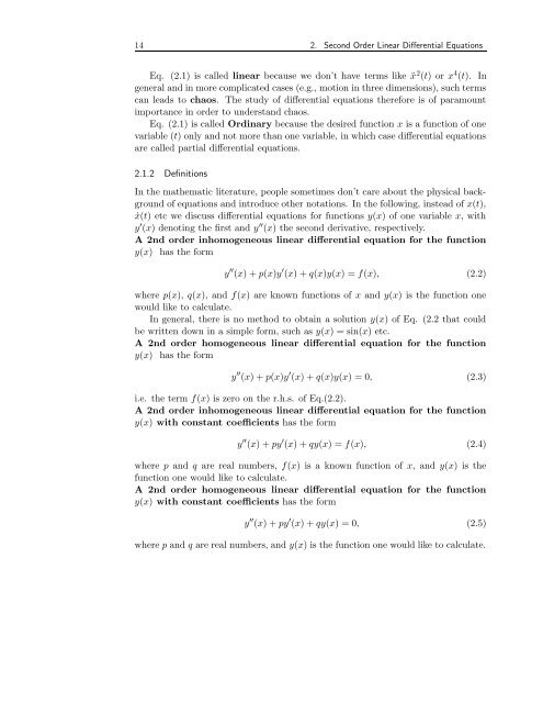
14 <strong>2.</strong> Second Order Linear Differential Equations<br />
Eq. (<strong>2.</strong>1) is called linear because we don’t have terms like ¨x 2 (t) or x 4 (t). In<br />
general and in more complicated cases (e.g., motion in three dimensions), such terms<br />
can leads to chaos. The study of differential equations therefore is of paramount<br />
importance in order to understand chaos.<br />
Eq. (<strong>2.</strong>1) is called Ordinary because the desired function x is a function of one<br />
variable (t) only and not more than one variable, in which case differential equations<br />
are called partial differential equations.<br />
<strong>2.</strong>1.2 Definitions<br />
In the mathematic literature, people sometimes don’t care about the physical background<br />
of equations and introduce other notations. In the following, instead of x(t),<br />
˙x(t) etc we discuss differential equations for functions y(x) of one variable x, with<br />
y ′ (x) denoting the first and y ′′ (x) the second derivative, respectively.<br />
A 2nd order inhomogeneous linear differential equation for the function<br />
y(x) has the form<br />
y ′′ (x) + p(x)y ′ (x) + q(x)y(x) = f(x), (<strong>2.</strong>2)<br />
where p(x), q(x), and f(x) are known functions of x and y(x) is the function one<br />
would like to calculate.<br />
In general, there is no method to obtain a solution y(x) of Eq. (<strong>2.</strong>2 that could<br />
be written down in a simple form, such as y(x) = sin(x) etc.<br />
A 2nd order homogeneous linear differential equation for the function<br />
y(x) has the form<br />
y ′′ (x) + p(x)y ′ (x) + q(x)y(x) = 0, (<strong>2.</strong>3)<br />
i.e. the term f(x) is zero on the r.h.s. of Eq.(<strong>2.</strong>2).<br />
A 2nd order inhomogeneous linear differential equation for the function<br />
y(x) with constant coefficients has the form<br />
y ′′ (x) + py ′ (x) + qy(x) = f(x), (<strong>2.</strong>4)<br />
where p and q are real numbers, f(x) is a known function of x, and y(x) is the<br />
function one would like to calculate.<br />
A 2nd order homogeneous linear differential equation for the function<br />
y(x) with constant coefficients has the form<br />
y ′′ (x) + py ′ (x) + qy(x) = 0, (<strong>2.</strong>5)<br />
where p and q are real numbers, and y(x) is the function one would like to calculate.