- Page 1 and 2:
James E. Gentle Theory of Statistic
- Page 3 and 4:
Preface: Mathematical Statistics Af
- Page 5 and 6:
Preface vii The objective in the di
- Page 7 and 8:
x = ⎛ ⎜ ⎝ x1 . xd ⎞ ⎟ ⎠
- Page 9 and 10:
• State and prove Fatou’s lemma
- Page 11 and 12:
Contents Preface . . . . . . . . .
- Page 13 and 14:
Contents xv 2.10 Multivariate Distr
- Page 15 and 16:
Contents xvii 5.2.1 Expectation Fun
- Page 17 and 18:
Contents xix 8.5.1 Nonparametric Pr
- Page 19 and 20:
1 Probability Theory Probability th
- Page 21 and 22:
1.1 Some Important Probability Fact
- Page 23 and 24:
1.1 Some Important Probability Fact
- Page 25 and 26:
Definition 1.8 (exchangeability) Le
- Page 27 and 28:
1.1 Some Important Probability Fact
- Page 29 and 30:
1.1 Some Important Probability Fact
- Page 31 and 32:
1.1 Some Important Probability Fact
- Page 33 and 34:
Theorem 1.5 (properties of a CDF) I
- Page 35 and 36:
1.1 Some Important Probability Fact
- Page 37 and 38:
1.1 Some Important Probability Fact
- Page 39 and 40:
.5 PDF p X(x;θ) 0 x θ=1 θ=5 1.1
- Page 41 and 42:
Joint and Marginal Distributions 1.
- Page 43 and 44:
1.1 Some Important Probability Fact
- Page 45 and 46:
1.1 Some Important Probability Fact
- Page 47 and 48:
1.1 Some Important Probability Fact
- Page 49 and 50:
1.1 Some Important Probability Fact
- Page 51 and 52:
1.1 Some Important Probability Fact
- Page 53 and 54:
1.1 Some Important Probability Fact
- Page 55 and 56:
1.1 Some Important Probability Fact
- Page 57 and 58:
1.1 Some Important Probability Fact
- Page 59 and 60:
1.1 Some Important Probability Fact
- Page 61 and 62:
Moment-Generating Functions 1.1 Som
- Page 63 and 64:
1.1 Some Important Probability Fact
- Page 65 and 66:
1.1 Some Important Probability Fact
- Page 67 and 68:
1.1 Some Important Probability Fact
- Page 69 and 70:
A Taylor series expansion of this g
- Page 71 and 72:
1.1 Some Important Probability Fact
- Page 73 and 74:
1.1 Some Important Probability Fact
- Page 75 and 76:
1.1 Some Important Probability Fact
- Page 77 and 78:
1.1 Some Important Probability Fact
- Page 79 and 80:
1.1 Some Important Probability Fact
- Page 81 and 82:
1.1 Some Important Probability Fact
- Page 83 and 84:
1.2 Series Expansions 65 X is the u
- Page 85 and 86:
κ1 = E(Z) κ2 = E(Z 2 ) − (E(Z))
- Page 87 and 88:
1.3 Sequences of Events and of Rand
- Page 89 and 90:
1.3 Sequences of Events and of Rand
- Page 91 and 92:
1.3 Sequences of Events and of Rand
- Page 93 and 94:
1.3 Sequences of Events and of Rand
- Page 95 and 96:
We write 1.3 Sequences of Events an
- Page 97 and 98:
1.3 Sequences of Events and of Rand
- Page 99 and 100:
1.3 Sequences of Events and of Rand
- Page 101 and 102:
1.3 Sequences of Events and of Rand
- Page 103 and 104:
1.3 Sequences of Events and of Rand
- Page 105 and 106:
1.3 Sequences of Events and of Rand
- Page 107 and 108:
1.3 Sequences of Events and of Rand
- Page 109 and 110:
1.3.6 Convergence of Functions 1.3
- Page 111 and 112:
1.3 Sequences of Events and of Rand
- Page 113 and 114:
1.3 Sequences of Events and of Rand
- Page 115 and 116:
1.3 Sequences of Events and of Rand
- Page 117 and 118:
we have for fixed k, 1.3 Sequences
- Page 119 and 120:
Multivariate Asymptotic Expectation
- Page 121 and 122:
1.4 Limit Theorems 103 The bn can b
- Page 123 and 124:
1.4 Limit Theorems 105 it applies t
- Page 125 and 126:
lim n→∞ max σ j≤kn 2 nj σ2
- Page 127 and 128:
1.5 Conditional Probability 109 The
- Page 129 and 130:
Conditional Expectation over a Sub-
- Page 131 and 132:
• monotone convergence: for 0 ≤
- Page 133 and 134:
Fn(t) = ⌊nt⌋ + 1 n + 1 ; 1.5 Co
- Page 135 and 136:
1.5 Conditional Probability 117 If
- Page 137 and 138:
1.5 Conditional Probability 119 1.5
- Page 139 and 140:
Conditional Entropy 1.6 Stochastic
- Page 141 and 142:
1.6 Stochastic Processes 123 Stoppi
- Page 143 and 144:
1.6 Stochastic Processes 125 (Exerc
- Page 145 and 146:
1.6 Stochastic Processes 127 variab
- Page 147 and 148:
1.6 Stochastic Processes 129 in a d
- Page 149 and 150:
1.6 Stochastic Processes 131 We als
- Page 151 and 152:
1.6 Stochastic Processes 133 X0 has
- Page 153 and 154:
Convergence of Empirical Processes
- Page 155 and 156:
and Fn(x, ω) ≥ Fn(xm,k−1, ω)
- Page 157 and 158:
Notes and Further Reading 139 and f
- Page 159 and 160:
Notes and Further Reading 141 we ca
- Page 161 and 162:
Notes and Further Reading 143 After
- Page 163 and 164:
Exercises 145 of betting system. Do
- Page 165 and 166:
Exercises 147 1.22. Show that if th
- Page 167 and 168:
1.36. Consider the the distribution
- Page 169 and 170:
Exercises 151 1.59. A sufficient co
- Page 171 and 172:
Exercises 153 1.85. Show that Doob
- Page 173 and 174:
2 Distribution Theory and Statistic
- Page 175 and 176:
2 Distribution Theory and Statistic
- Page 177 and 178:
2 Distribution Theory and Statistic
- Page 179 and 180:
2 Distribution Theory and Statistic
- Page 181 and 182:
Example 2.1 complete and incomplete
- Page 183 and 184:
2.2 Shapes of the Probability Densi
- Page 185 and 186:
2.2 Shapes of the Probability Densi
- Page 187 and 188:
2.3.2 The Le Cam Regularity Conditi
- Page 189 and 190:
2.4 The Exponential Class of Famili
- Page 191 and 192:
2.4 The Exponential Class of Famili
- Page 193 and 194:
2.4 The Exponential Class of Famili
- Page 195 and 196:
or or 2.5 Parametric-Support Famili
- Page 197 and 198:
2.6 Transformation Group Families 1
- Page 199 and 200:
2.6 Transformation Group Families 1
- Page 201 and 202:
2.7 Truncated and Censored Distribu
- Page 203 and 204:
2.9 Infinitely Divisible and Stable
- Page 205 and 206:
Higher Dimensions 2.11 The Family o
- Page 207 and 208:
2.11 The Family of Normal Distribut
- Page 209 and 210:
2.11 The Family of Normal Distribut
- Page 211 and 212:
2.11 The Family of Normal Distribut
- Page 213 and 214:
Exercises 195 are considered at som
- Page 215 and 216:
Exercises 197 This law has been use
- Page 217 and 218:
Exercises 199 a) Show that for d
- Page 219 and 220:
3 Basic Statistical Theory The fiel
- Page 221 and 222:
How Does PH Differ from P? 3 Basic
- Page 223 and 224:
3 Basic Statistical Theory 205 abov
- Page 225 and 226:
3.1 Inferential Information in Stat
- Page 227 and 228:
3.1 Inferential Information in Stat
- Page 229 and 230:
3.1 Inferential Information in Stat
- Page 231 and 232:
The Basic Paradigm of Point Estimat
- Page 233 and 234:
3.1 Inferential Information in Stat
- Page 235 and 236:
3.1 Inferential Information in Stat
- Page 237 and 238:
3.1 Inferential Information in Stat
- Page 239 and 240:
Completeness 3.1 Inferential Inform
- Page 241 and 242:
and so by completeness, 3.1 Inferen
- Page 243 and 244:
3.1 Inferential Information in Stat
- Page 245 and 246:
and so I(µ, σ) = Eθ = E(µ,σ) =
- Page 247 and 248:
3.1 Inferential Information in Stat
- Page 249 and 250:
3.1 Inferential Information in Stat
- Page 251 and 252:
Robustness 3.1 Inferential Informat
- Page 253 and 254:
3.2 Statistical Inference: Approach
- Page 255 and 256:
3.2 Statistical Inference: Approach
- Page 257 and 258:
3.2 Statistical Inference: Approach
- Page 259 and 260:
3.2 Statistical Inference: Approach
- Page 261 and 262:
3.2 Statistical Inference: Approach
- Page 263 and 264:
3.2 Statistical Inference: Approach
- Page 265 and 266:
3.2 Statistical Inference: Approach
- Page 267 and 268:
3.2 Statistical Inference: Approach
- Page 269 and 270:
3.2 Statistical Inference: Approach
- Page 271 and 272:
3.2 Statistical Inference: Approach
- Page 273 and 274:
3.3 The Decision Theory Approach to
- Page 275 and 276:
3.3 The Decision Theory Approach to
- Page 277 and 278:
3.3 The Decision Theory Approach to
- Page 279 and 280:
3.3 The Decision Theory Approach to
- Page 281 and 282:
3.3 The Decision Theory Approach to
- Page 283 and 284:
3.3 The Decision Theory Approach to
- Page 285 and 286:
3.3 The Decision Theory Approach to
- Page 287 and 288:
3.3 The Decision Theory Approach to
- Page 289 and 290:
3.3 The Decision Theory Approach to
- Page 291 and 292:
Risk 0.005 0.010 0.015 0.020 0.025
- Page 293 and 294:
3.4 Invariant and Equivariant Stati
- Page 295 and 296:
3.4 Invariant and Equivariant Stati
- Page 297 and 298:
3.4 Invariant and Equivariant Stati
- Page 299 and 300:
Equivariant Point Estimation 3.4 In
- Page 301 and 302:
3.4 Invariant and Equivariant Stati
- Page 303 and 304:
3.4 Invariant and Equivariant Stati
- Page 305 and 306:
3.5 Probability Statements in Stati
- Page 307 and 308:
Test Rules 3.5 Probability Statemen
- Page 309 and 310:
3.5 Probability Statements in Stati
- Page 311 and 312:
3.5 Probability Statements in Stati
- Page 313 and 314:
3.5 Probability Statements in Stati
- Page 315 and 316:
if 3.6 Variance Estimation 297 Give
- Page 317 and 318:
3.6 Variance Estimation 299 J(T) =
- Page 319 and 320:
3.7 Applications 3.7.1 Inference in
- Page 321 and 322:
3.8 Asymptotic Inference 303 The ca
- Page 323 and 324:
3.8 Asymptotic Inference 305 The mo
- Page 325 and 326:
3.8 Asymptotic Inference 307 wherea
- Page 327 and 328:
3.8 Asymptotic Inference 309 tendin
- Page 329 and 330:
Definition 3.20 (asymptotic signifi
- Page 331 and 332:
Proof. *************** Notes and Fu
- Page 333 and 334:
Notes and Further Reading 315 Least
- Page 335 and 336:
Approximations and Asymptotic Infer
- Page 337 and 338:
Exercises 319 b) the expectation of
- Page 339 and 340:
4 Bayesian Inference We have used a
- Page 341 and 342:
4.1 The Bayesian Paradigm 323 For m
- Page 343 and 344:
4.1 The Bayesian Paradigm 325 A qua
- Page 345 and 346:
4.2 Bayesian Analysis 327 even if t
- Page 347 and 348:
4.2 Bayesian Analysis 329 Hence P(B
- Page 349 and 350:
4.2 Bayesian Analysis 331 B1. ∀θ
- Page 351 and 352:
4.2 Bayesian Analysis 333 This mean
- Page 353 and 354:
Prior Prior 0.0 0.5 1.0 1.5 2.0 0 2
- Page 355 and 356:
4.2 Bayesian Analysis 337 We go thr
- Page 357 and 358:
4.2 Bayesian Analysis 339 We constr
- Page 359 and 360:
4.2 Bayesian Analysis 341 as the mo
- Page 361 and 362:
Assessing the Problem Formulation 4
- Page 363 and 364:
Posterior Posterior 0 5 10 15 0 1 2
- Page 365 and 366:
4.2 Bayesian Analysis 347 distribut
- Page 367 and 368:
4.3 Bayes Rules 349 • the nature
- Page 369 and 370:
Then we have E(g(θ)T(X)) = E(T(X)E
- Page 371 and 372:
4.3 Bayes Rules 353 equivariance Fo
- Page 373 and 374:
4.3 Bayes Rules 355 Example 4.9 (Co
- Page 375 and 376:
4.4 Probability Statements in Stati
- Page 377 and 378:
p0 = Pr(Θ ∈ Θ0) and p1 = Pr(Θ
- Page 379 and 380:
The Weighted 0-1 or α0-α1 Loss Fu
- Page 381 and 382:
The term ˆp0 ˆp1 = p0 p1 BF(x) =
- Page 383 and 384:
4.5 Bayesian Testing 365 • Bayes
- Page 385 and 386:
where fΘ|x(θ|x) = p1 if θ = θ0
- Page 387 and 388:
4.6 Bayesian Confidence Sets 369 as
- Page 389 and 390:
Posterior 0 1 2 3 95% Credible Regi
- Page 391 and 392:
Markov Chain Monte Carlo 4.7 Comput
- Page 393 and 394:
4.7 Computational Methods 375 β/(t
- Page 395 and 396:
Notes and Further Reading 377 An al
- Page 397 and 398:
4.4. Given the conditional PDF a) U
- Page 399 and 400:
Exercises 381 4.14. Consider again
- Page 401 and 402:
Exercises 383 4.26. As in Exercise
- Page 403 and 404:
5 Unbiased Point Estimation In a de
- Page 405 and 406:
Estimability 5 Unbiased Point Estim
- Page 407 and 408:
s1π + s0(1 − π) = π, 5.1 UMVUE
- Page 409 and 410:
5.1 UMVUE 391 Let T be UMVUE for g(
- Page 411 and 412:
5.1 UMVUE 393 Example 5.7 UMVUE of
- Page 413 and 414:
5.1 UMVUE 395 The risk of T ∗ is
- Page 415 and 416:
5.1 UMVUE 397 estimator of θ that
- Page 417 and 418:
(Compare this with Tfdx = g(θ).)
- Page 419 and 420:
¯h(X1, . . ., Xm) = 1 m! 5.2 U-Sta
- Page 421 and 422:
where Pn is the ECDF. U(X1, . . .,
- Page 423 and 424:
and T 2 r,S = C = Tr,S = C C TnT
- Page 425 and 426:
Generalized U-Statistics 5.2 U-Stat
- Page 427 and 428:
5.2 U-Statistics 409 Theorem 5.4 (H
- Page 429 and 430:
5.3 Asymptotically Unbiased Estimat
- Page 431 and 432:
5.3.2 Ratio Estimators 5.3 Asymptot
- Page 433 and 434:
5.4 Asymptotic Efficiency 415 of a
- Page 435 and 436:
⎧ ⎨ Tn = ⎩ n2 with probabilit
- Page 437 and 438:
5.5 Applications 5.5 Applications 4
- Page 439 and 440:
5.5 Applications 421 one aspect of
- Page 441 and 442:
Proof. Because l ∈ span(X T ) = s
- Page 443 and 444:
Optimal Properties of the Moore-Pen
- Page 445 and 446:
5.5 Applications 427 implies implie
- Page 447 and 448:
The “Sum of Squares” Quadratic
- Page 449 and 450:
5.5 Applications 431 The question o
- Page 451 and 452:
We now write the original model as
- Page 453 and 454:
5.5 Applications 435 it from other
- Page 455 and 456:
(it’s Bernoulli), and for i = j,
- Page 457 and 458:
Fisher Efficient Estimators and Exp
- Page 459 and 460:
6 Statistical Inference Based on Li
- Page 461 and 462:
6.1 The Likelihood Function 443 is
- Page 463 and 464:
6.2 Maximum Likelihood Parametric E
- Page 465 and 466:
6.2 Maximum Likelihood Parametric E
- Page 467 and 468:
6.2 Maximum Likelihood Parametric E
- Page 469 and 470:
6.2 Maximum Likelihood Parametric E
- Page 471 and 472:
6.2.2 Finite Sample Properties of M
- Page 473 and 474:
6.2 Maximum Likelihood Parametric E
- Page 475 and 476:
6.2 Maximum Likelihood Parametric E
- Page 477 and 478:
6.2 Maximum Likelihood Parametric E
- Page 479 and 480:
6.2 Maximum Likelihood Parametric E
- Page 481 and 482:
6.2 Maximum Likelihood Parametric E
- Page 483 and 484:
6.2 Maximum Likelihood Parametric E
- Page 485 and 486:
6.2 Maximum Likelihood Parametric E
- Page 487 and 488:
6.2 Maximum Likelihood Parametric E
- Page 489 and 490:
6.2 Maximum Likelihood Parametric E
- Page 491 and 492:
where Now, consider This has two pa
- Page 493 and 494:
6.2 Maximum Likelihood Parametric E
- Page 495 and 496:
6.3 Asymptotic Properties of MLEs,
- Page 497 and 498:
6.3 Asymptotic Properties of MLEs,
- Page 499 and 500:
6.3 Asymptotic Properties of MLEs,
- Page 501 and 502:
6.4 Application: MLEs in Generalize
- Page 503 and 504:
6.4 Application: MLEs in Generalize
- Page 505 and 506: 6.4 Application: MLEs in Generalize
- Page 507 and 508: 6.4 Application: MLEs in Generalize
- Page 509 and 510: 6.4 Application: MLEs in Generalize
- Page 511 and 512: Residuals 6.4 Application: MLEs in
- Page 513 and 514: 6.5 Variations on the Likelihood 49
- Page 515 and 516: 6.5 Variations on the Likelihood 49
- Page 517 and 518: Maximum Likelihood in Linear Models
- Page 519 and 520: Exercises 501 b) Assume that σ 2 1
- Page 521 and 522: 7 Statistical Hypotheses and Confid
- Page 523 and 524: Tests of Hypotheses 7.1 Statistical
- Page 525 and 526: 7.1 Statistical Hypotheses 507 Know
- Page 527 and 528: Power of a Statistical Test 7.1 Sta
- Page 529 and 530: An Optimal Test in a Simple Situati
- Page 531 and 532: 7.2 Optimal Tests 513 All of these
- Page 533 and 534: Use of Sufficient Statistics 7.2 Op
- Page 535 and 536: 7.2 Optimal Tests 517 Syppose we as
- Page 537 and 538: Nonexistence of UMP Tests 7.2 Optim
- Page 539 and 540: H0 : θ = θ0 versus H1 : θ = θ0.
- Page 541 and 542: 7.2.6 Equivariance, Unbiasedness, a
- Page 543 and 544: 7.3 Likelihood Ratio Tests, Wald Te
- Page 545 and 546: 7.3 Likelihood Ratio Tests, Wald Te
- Page 547 and 548: Minimize 7.3 Likelihood Ratio Tests
- Page 549 and 550: 7.4 Nonparametric Tests 531 I(0, ˆ
- Page 551 and 552: Yij = µ + αi + ɛij, i = 1, . . .
- Page 553 and 554: 7.7 The Likelihood Principle and Te
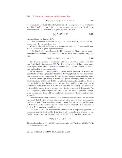
- Page 555: 7.8 Confidence Sets 537 Monte Carlo
- Page 559 and 560: 7.8 Confidence Sets 541 For any giv
- Page 561 and 562: 7.9 Optimal Confidence Sets 543 Thi
- Page 563 and 564: 7.9 Optimal Confidence Sets 545 Con
- Page 565 and 566: 7.10 Asymptotic Confidence sets 547
- Page 567 and 568: 7.11 Bootstrap Confidence Sets 549
- Page 569 and 570: Bias in Intervals Due to Bias in th
- Page 571 and 572: 7.12 Simultaneous Confidence Sets 5
- Page 573 and 574: Sequential Tests Exercises 555 Wald
- Page 575 and 576: 8 Nonparametric and Robust Inferenc
- Page 577 and 578: 8.2 Inference Based on Order Statis
- Page 579 and 580: f ^ (x) Nonparametric Regression 0.
- Page 581 and 582: 8.3 Nonparametric Estimation of Fun
- Page 583 and 584: 8.3 Nonparametric Estimation of Fun
- Page 585 and 586: 8.3 Nonparametric Estimation of Fun
- Page 587 and 588: 8.3 Nonparametric Estimation of Fun
- Page 589 and 590: ISE θ = 8.3 Nonparametric Estim
- Page 591 and 592: 8.4 Semiparametric Methods and Part
- Page 593 and 594: 8.5 Nonparametric Estimation of PDF
- Page 595 and 596: 8.5 Nonparametric Estimation of PDF
- Page 597 and 598: Some Properties of the Histogram Es
- Page 599 and 600: 8.5 Nonparametric Estimation of PDF
- Page 601 and 602: AISB 1 pH = 12 8.5 Nonparametric
- Page 603 and 604: and the integrated variance is 8.5
- Page 605 and 606: and 8.5 Nonparametric Estimation o
- Page 607 and 608:
h ∗ = 8.5 Nonparametric Estimatio
- Page 609 and 610:
Computation of Kernel Density Estim
- Page 611 and 612:
8.6 Perturbations of Probability Di
- Page 613 and 614:
CDF 0.0 0.2 0.4 0.6 0.8 1.0 1.2 1.4
- Page 615 and 616:
8.6 Perturbations of Probability Di
- Page 617 and 618:
8.7 Robust Inference 8.7 Robust Inf
- Page 619 and 620:
p(y) (1-ε)p(y) The Influence Funct
- Page 621 and 622:
8.7 Robust Inference 603 Notice tha
- Page 623 and 624:
Nonparametric Statistics Exercises
- Page 625 and 626:
0 Statistical Mathematics Statistic
- Page 627 and 628:
0 Statistical Mathematics 609 x may
- Page 629 and 630:
0.0 Some Basic Mathematical Concept
- Page 631 and 632:
Because each is a subset of the oth
- Page 633 and 634:
0.0.2 Sets and Spaces 0.0 Some Basi
- Page 635 and 636:
0.0.2.4 Point Sequences in a Topolo
- Page 637 and 638:
0.0 Some Basic Mathematical Concept
- Page 639 and 640:
The sequence of sets {An} is said t
- Page 641 and 642:
0.0 Some Basic Mathematical Concept
- Page 643 and 644:
0.0 Some Basic Mathematical Concept
- Page 645 and 646:
0.0 Some Basic Mathematical Concept
- Page 647 and 648:
0.0 Some Basic Mathematical Concept
- Page 649 and 650:
The proof of this is a classic: fir
- Page 651 and 652:
0.0 Some Basic Mathematical Concept
- Page 653 and 654:
• ∀x ∈ IR ∪ {∞}, x × ±
- Page 655 and 656:
0.0 Some Basic Mathematical Concept
- Page 657 and 658:
0.0.5.2 Sets of Reals; Open, Closed
- Page 659 and 660:
0.0 Some Basic Mathematical Concept
- Page 661 and 662:
0.0 Some Basic Mathematical Concept
- Page 663 and 664:
We have 0.0 Some Basic Mathematical
- Page 665 and 666:
0.0 Some Basic Mathematical Concept
- Page 667 and 668:
0.0 Some Basic Mathematical Concept
- Page 669 and 670:
0.0 Some Basic Mathematical Concept
- Page 671 and 672:
Definition 0.0.14 (superharmonic fu
- Page 673 and 674:
0.0 Some Basic Mathematical Concept
- Page 675 and 676:
Ordering the Complex Numbers 0.0 So
- Page 677 and 678:
0.0 Some Basic Mathematical Concept
- Page 679 and 680:
0.0 Some Basic Mathematical Concept
- Page 681 and 682:
0.0 Some Basic Mathematical Concept
- Page 683 and 684:
0.0 Some Basic Mathematical Concept
- Page 685 and 686:
0.0 Some Basic Mathematical Concept
- Page 687 and 688:
0.0 Some Basic Mathematical Concept
- Page 689 and 690:
0.0 Some Basic Mathematical Concept
- Page 691 and 692:
0.0.9.5 Working with Real-Valued Fu
- Page 693 and 694:
∞ 0.0 Some Basic Mathematical Con
- Page 695 and 696:
0.0 Some Basic Mathematical Concept
- Page 697 and 698:
0.0 Some Basic Mathematical Concept
- Page 699 and 700:
0.0 Some Basic Mathematical Concept
- Page 701 and 702:
0.0 Some Basic Mathematical Concept
- Page 703 and 704:
a) Evaluate the integral (0.0.84):
- Page 705 and 706:
0.1 Measure, Integration, and Funct
- Page 707 and 708:
0.1 Measure, Integration, and Funct
- Page 709 and 710:
0.1 Measure, Integration, and Funct
- Page 711 and 712:
0.1 Measure, Integration, and Funct
- Page 713 and 714:
0.1 Measure, Integration, and Funct
- Page 715 and 716:
0.1 Measure, Integration, and Funct
- Page 717 and 718:
3. if A1, A2, . . . ∈ F are disjo
- Page 719 and 720:
0.1 Measure, Integration, and Funct
- Page 721 and 722:
0.1 Measure, Integration, and Funct
- Page 723 and 724:
0.1 Measure, Integration, and Funct
- Page 725 and 726:
0.1 Measure, Integration, and Funct
- Page 727 and 728:
0.1 Measure, Integration, and Funct
- Page 729 and 730:
0.1 Measure, Integration, and Funct
- Page 731 and 732:
(why?), and so We also have λ 0.1
- Page 733 and 734:
0.1 Measure, Integration, and Funct
- Page 735 and 736:
0.1 Measure, Integration, and Funct
- Page 737 and 738:
0.1 Measure, Integration, and Funct
- Page 739 and 740:
0.1 Measure, Integration, and Funct
- Page 741 and 742:
Proof. Exercise. 0.1 Measure, Integ
- Page 743 and 744:
Hence, from inequality (0.1.47),
- Page 745 and 746:
0.1 Measure, Integration, and Funct
- Page 747 and 748:
0.1 Measure, Integration, and Funct
- Page 749 and 750:
0.1 Measure, Integration, and Funct
- Page 751 and 752:
0.1 Measure, Integration, and Funct
- Page 753 and 754:
0.1 Measure, Integration, and Funct
- Page 755 and 756:
0.1.9.3 Norms of Functions 0.1 Meas
- Page 757 and 758:
0.1 Measure, Integration, and Funct
- Page 759 and 760:
0.1 Measure, Integration, and Funct
- Page 761 and 762:
0.1 Measure, Integration, and Funct
- Page 763 and 764:
0.1 Measure, Integration, and Funct
- Page 765 and 766:
0.1 Measure, Integration, and Funct
- Page 767 and 768:
0.1.12 Transforms 0.1 Measure, Inte
- Page 769 and 770:
0.1 Measure, Integration, and Funct
- Page 771 and 772:
0.1 Measure, Integration, and Funct
- Page 773 and 774:
0.1 Measure, Integration, and Funct
- Page 775 and 776:
0.2 Stochastic Processes and the St
- Page 777 and 778:
0.2 Stochastic Processes and the St
- Page 779 and 780:
Variation of Functionals 0.2 Stocha
- Page 781 and 782:
0.2 Stochastic Processes and the St
- Page 783 and 784:
0.2.1.3 Ito Processes 0.2 Stochasti
- Page 785 and 786:
0.2 Stochastic Processes and the St
- Page 787 and 788:
0.2.2.2 Ito’s Lemma 0.2 Stochasti
- Page 789 and 790:
0.2 Stochastic Processes and the St
- Page 791 and 792:
0.3 Some Basics of Linear Algebra 0
- Page 793 and 794:
0.3 Some Basics of Linear Algebra 7
- Page 795 and 796:
0.3.2.2 The Trace and Some of Its P
- Page 797 and 798:
0.3 Some Basics of Linear Algebra 7
- Page 799 and 800:
The Fourier Expansion 0.3 Some Basi
- Page 801 and 802:
0.3 Some Basics of Linear Algebra 7
- Page 803 and 804:
0.3 Some Basics of Linear Algebra 7
- Page 805 and 806:
0.3.2.8 Spectral Decomposition 0.3
- Page 807 and 808:
0.3.2.11 Inverses of Matrices 0.3 S
- Page 809 and 810:
0.3 Some Basics of Linear Algebra 7
- Page 811 and 812:
0.3 Some Basics of Linear Algebra 7
- Page 813 and 814:
0.3 Some Basics of Linear Algebra 7
- Page 815 and 816:
we have 0.3 Some Basics of Linear A
- Page 817 and 818:
0.3 Some Basics of Linear Algebra 7
- Page 819 and 820:
0.3 Some Basics of Linear Algebra 8
- Page 821 and 822:
0.3 Some Basics of Linear Algebra 8
- Page 823 and 824:
f(x) ≈ f(x∗) + (x − x∗) T
- Page 825 and 826:
0.3 Some Basics of Linear Algebra 8
- Page 827 and 828:
0.3 Some Basics of Linear Algebra 8
- Page 829 and 830:
and so E T π (I + A) n−1 Eπ =
- Page 831 and 832:
0.3 Some Basics of Linear Algebra 8
- Page 833 and 834:
0.4.1.2 Methods 0.4 Optimization 81
- Page 835 and 836:
0.4.1.7 The Steps in Iterative Algo
- Page 837 and 838:
0.4.1.11 Modifications of Newton’
- Page 839 and 840:
We generally require g x (k) ; x (
- Page 841 and 842:
0.4 Optimization 823 3. Generate st
- Page 843 and 844:
Theory of Statistics c○2000-2013
- Page 845 and 846:
A Important Probability Distributio
- Page 847 and 848:
Appendix A. Important Probability D
- Page 849 and 850:
Appendix A. Important Probability D
- Page 851 and 852:
Appendix A. Important Probability D
- Page 853 and 854:
Appendix A. Important Probability D
- Page 855 and 856:
B Useful Inequalities in Probabilit
- Page 857 and 858:
B.3 Pr(X ∈ A) and E(f(X)) 839 Pr(
- Page 859 and 860:
B.4 E(f(X)) and f(E(X)) 841 Theorem
- Page 861 and 862:
B.4 E(f(X)) and f(E(X)) 843 A relat
- Page 863 and 864:
B.5 E(f(X,Y )) and E(g(X)) and E(h(
- Page 865 and 866:
Now assume p > 1. Now, E(|X + Y | p
- Page 867 and 868:
C Notation and Definitions All nota
- Page 869 and 870:
C.1 General Notation 851 constant;
- Page 871 and 872:
C.2 General Mathematical Functions
- Page 873 and 874:
Functions of Convenience C.2 Genera
- Page 875 and 876:
C.2 General Mathematical Functions
- Page 877 and 878:
A1 ∩ A2 A1 − A2 A1∆A2 A1 × A
- Page 879 and 880:
C.4 Linear Spaces and Matrices 861
- Page 881 and 882:
a(ij) C.4 Linear Spaces and Matrice
- Page 883 and 884:
References The number(s) following
- Page 885 and 886:
References 867 Lyle D. Broemeling.
- Page 887 and 888:
References 869 William Feller. An I
- Page 889 and 890:
References 871 H. O. Hartley. In Dr
- Page 891 and 892:
References 873 Feldman, and Murad S
- Page 893 and 894:
References 875 Roger B. Nelsen. An
- Page 895 and 896:
References 877 Glenn Shafer. A Math
- Page 897 and 898:
References 879 Abraham Wald. Sequen
- Page 899 and 900:
Index a.e. (almost everywhere), 704
- Page 901 and 902:
cartesian product measurable space,
- Page 903 and 904:
derivative of a functional, 752-753
- Page 905 and 906:
Euclidean norm, 774 Euler’s formu
- Page 907 and 908:
unbiased test, 292, 519 uniform con
- Page 909 and 910:
sequence of sets, 620-623 limit poi
- Page 911 and 912:
natural parameter space, 173 neglig
- Page 913 and 914:
proportional hazards, 573 pseudoinv
- Page 915 and 916:
square root matrix, 783 squared-err
- Page 917:
weak convergence in mean square, 56