Measuring the Effects of a Shock to Monetary Policy - Humboldt ...
Measuring the Effects of a Shock to Monetary Policy - Humboldt ...
Measuring the Effects of a Shock to Monetary Policy - Humboldt ...
Create successful ePaper yourself
Turn your PDF publications into a flip-book with our unique Google optimized e-Paper software.
Bayesian FAVARs with Agnostic Identification 21<br />
F ∗<br />
t = AFt − BYt<br />
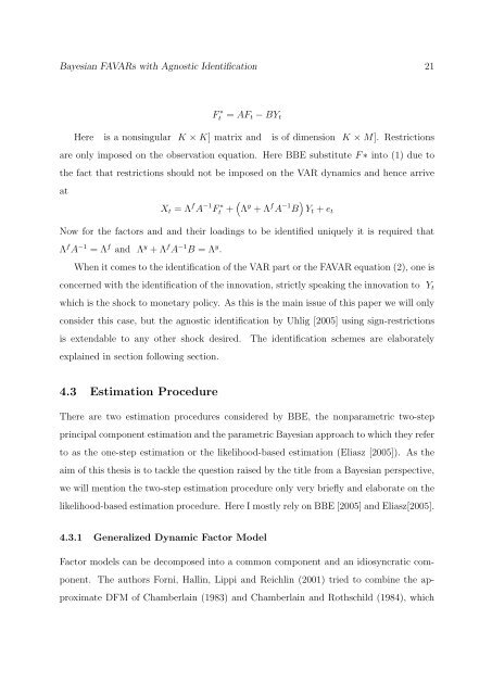
Here is a nonsingular K × K] matrix and is <strong>of</strong> dimension K × M]. Restrictions<br />
are only imposed on <strong>the</strong> observation equation. Here BBE substitute F ∗ in<strong>to</strong> (1) due <strong>to</strong><br />
<strong>the</strong> fact that restrictions should not be imposed on <strong>the</strong> VAR dynamics and hence arrive<br />
at<br />
Xt = Λ f A −1 F ∗<br />
t + <br />
Λ y + Λ f A −1 B <br />
Yt + et<br />
Now for <strong>the</strong> fac<strong>to</strong>rs and and <strong>the</strong>ir loadings <strong>to</strong> be identified uniquely it is required that<br />
Λ f A −1 = Λ f and Λ y + Λ f A −1 B = Λ y .<br />
When it comes <strong>to</strong> <strong>the</strong> identification <strong>of</strong> <strong>the</strong> VAR part or <strong>the</strong> FAVAR equation (2), one is<br />
concerned with <strong>the</strong> identification <strong>of</strong> <strong>the</strong> innovation, strictly speaking <strong>the</strong> innovation <strong>to</strong> Yt<br />
which is <strong>the</strong> shock <strong>to</strong> monetary policy. As this is <strong>the</strong> main issue <strong>of</strong> this paper we will only<br />
consider this case, but <strong>the</strong> agnostic identification by Uhlig [2005] using sign-restrictions<br />
is extendable <strong>to</strong> any o<strong>the</strong>r shock desired. The identification schemes are elaborately<br />
explained in section following section.<br />
4.3 Estimation Procedure<br />
There are two estimation procedures considered by BBE, <strong>the</strong> nonparametric two-step<br />
principal component estimation and <strong>the</strong> parametric Bayesian approach <strong>to</strong> which <strong>the</strong>y refer<br />
<strong>to</strong> as <strong>the</strong> one-step estimation or <strong>the</strong> likelihood-based estimation (Eliasz [2005]). As <strong>the</strong><br />
aim <strong>of</strong> this <strong>the</strong>sis is <strong>to</strong> tackle <strong>the</strong> question raised by <strong>the</strong> title from a Bayesian perspective,<br />
we will mention <strong>the</strong> two-step estimation procedure only very briefly and elaborate on <strong>the</strong><br />
likelihood-based estimation procedure. Here I mostly rely on BBE [2005] and Eliasz[2005].<br />
4.3.1 Generalized Dynamic Fac<strong>to</strong>r Model<br />
Fac<strong>to</strong>r models can be decomposed in<strong>to</strong> a common component and an idiosyncratic com-<br />
ponent. The authors Forni, Hallin, Lippi and Reichlin (2001) tried <strong>to</strong> combine <strong>the</strong> ap-<br />
proximate DFM <strong>of</strong> Chamberlain (1983) and Chamberlain and Rothschild (1984), which







![[Text eingeben] [Text eingeben] Lebenslauf Anna-Maria Schneider](https://img.yumpu.com/16300391/1/184x260/text-eingeben-text-eingeben-lebenslauf-anna-maria-schneider.jpg?quality=85)
