Measuring the Effects of a Shock to Monetary Policy - Humboldt ...

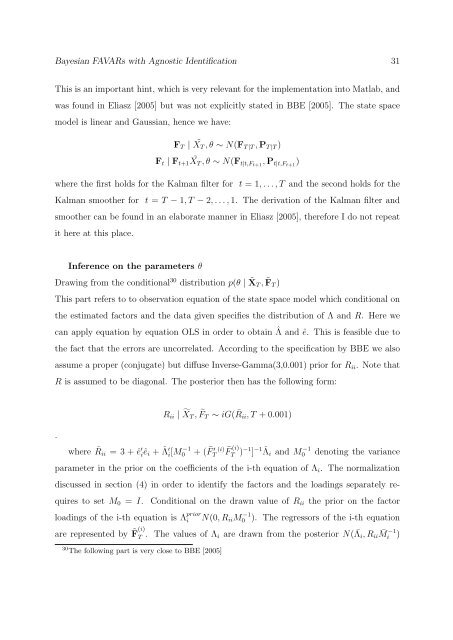
Bayesian FAVARs with Agnostic Identification 31
This is an important hint, which is very relevant for the implementation into Matlab, and
was found in Eliasz [2005] but was not explicitly stated in BBE [2005]. The state space
model is linear and Gaussian, hence we have:
FT | ˜
XT , θ ∼ N(FT |T , PT |T )
Ft | Ft+1 ˜
XT , θ ∼ N(Ft|t,Ft+1, Pt|t,Ft+1)
where the first holds for the Kalman filter for t = 1, . . . , T and the second holds for the
Kalman smoother for t = T − 1, T − 2, . . . , 1. The derivation of the Kalman filter and
smoother can be found in an elaborate manner in Eliasz [2005], therefore I do not repeat
it here at this place.
Inference on the parameters θ
Drawing from the conditional 30 distribution p(θ | ˜ XT , ˜ FT )
This part refers to to observation equation of the state space model which conditional on
the estimated factors and the data given specifies the distribution of Λ and R. Here we
can apply equation by equation OLS in order to obtain ˆ Λ and ê. This is feasible due to
the fact that the errors are uncorrelated. According to the specification by BBE we also
assume a proper (conjugate) but diffuse Inverse-Gamma(3,0.001) prior for Rii. Note that
R is assumed to be diagonal. The posterior then has the following form:
.
Rii | XT , FT ∼ iG( ¯ Rii, T + 0.001)
where ¯ Rii = 3 + ê ′ iêi + ˆ Λ ′ i[M −1
0 + ( F ′ T (i) F (i)
T ) −1 ] −1Λi ˆ and M −1
0
denoting the variance
parameter in the prior on the coefficients of the i-th equation of Λi. The normalization
discussed in section (4) in order to identify the factors and the loadings separately re-
quires to set M0 = I. Conditional on the drawn value of Rii the prior on the factor
loadings of the i-th equation is Λ prior
i N(0, RiiM −1
0 ). The regressors of the i-th equation
are represented by ˜ F (i)
T . The values of Λi are drawn from the posterior N( ¯ Λi, Rii ¯ M −1
i )
30 The following part is very close to BBE [2005]