Measuring the Effects of a Shock to Monetary Policy - Humboldt ...

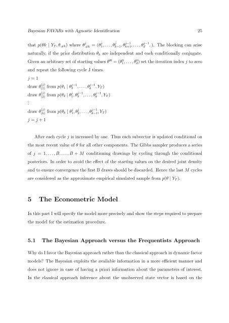
Bayesian FAVARs with Agnostic Identification 25
that p(θk | YT , θ.=k) where θ j
.=k
= (θj 1, . . . , θ j
k−1
, θj−1 k+1
, . . . , θj−1
d , ). The blocking can arise
naturally, if the prior distribution θk are independent and each conditionally conjugate.
Given an arbitrary set of starting values θ ′0 = (θ 0 1, . . . , θ 0 d) set the iteration index j to zero
and repeat the following cycle J times.
j = 1
draw θ (j)
(1) from p(θ1 | θ j−1
2 , . . . , θ j−1
k , YT )
draw θ (j)
(2) from p(θ2 | θ j
1, θ j−1
3 , . . . , θ j−1
k , YT )
.
draw θ (j)
(k) from p(θk | θ j
1, θ j
2, . . . , θ j−1
k−1 , YT )
j = j + 1
After each cycle j is increased by one. Thus each subvector is updated conditional on
the most recent value of θ for all other components. The Gibbs sampler produces a series
of j = 1, . . . , B, . . . , B + M conditioning drawings by cycling through the conditional
posteriors. In order to avoid the effect of the starting values on the desired joint density
and to ensure convergence the first B draws should be discarded. Hence the last M cycles
are considered as the approximate empirical simulated sample from p(θ | YT ).
5 The Econometric Model
In this part I will specify the model more precisely and show the steps required to prepare
the model for the estimation procedure.
5.1 The Bayesian Approach versus the Frequentists Approach
Why do I favor the Bayesian approach rather than the classical approach in dynamic factor
models? The Bayesian exploits the available information in a more efficient manner and
does not ignore in case of having a priori information about the parameters of interest.
In the classical approach inference about the unobserved state vector is based on the