Measuring the Effects of a Shock to Monetary Policy - Humboldt ...

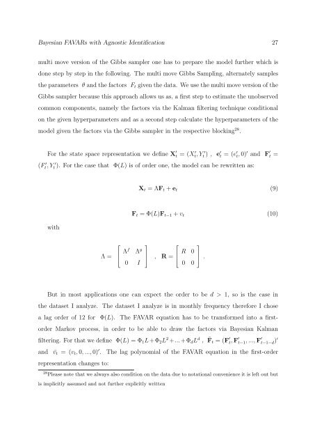
Bayesian FAVARs with Agnostic Identification 27
multi move version of the Gibbs sampler one has to prepare the model further which is
done step by step in the following. The multi move Gibbs Sampling, alternately samples
the parameters θ and the factors Ft given the data. We use the multi move version of the
Gibbs sampler because this approach allows us as, a first step to estimate the unobserved
common components, namely the factors via the Kalman filtering technique conditional
on the given hyperparameters and as a second step calculate the hyperparameters of the
model given the factors via the Gibbs sampler in the respective blocking 28 .
For the state space representation we define X ′
t = (X ′ t, Y ′
t ) , e ′ t = (e ′ t, 0) ′ and F ′
t =
(F ′
t, Y ′
t ). For the case that Φ(L) is of order one, the model can be rewritten as:
with
Λ =
⎡
⎢
⎣ Λf Λy 0 I
Xt = ΛFt + et
Ft = Φ(L)Ft−1 + vt
⎤
⎥
⎦ , R =
⎡
⎢
⎣
R 0
0 0
But in most applications one can expect the order to be d > 1, so is the case in
the dataset I analyze. The dataset I analyze is in monthly frequency therefore I chose
a lag order of 12 for Φ(L). The FAVAR equation has to be transformed into a first-
order Markov process, in order to be able to draw the factors via Bayesian Kalman
filtering. For that we define Φ(L) = Φ1L+Φ2L 2 +...+ΦdL d , ¯ Ft = (F ′
t, F ′
t−1, ..., F ′
t−1−d) ′
and ¯vt = (vt, 0, ..., 0) ′ . The lag polynomial of the FAVAR equation in the first-order
representation changes to:
28 Please note that we always also condition on the data due to notational convenience it is left out but
is implicitly assumed and not further explicitly written
⎤
⎥
⎦ .
(9)
(10)