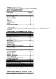
Measuring the Effects of a Shock to Monetary Policy - Humboldt ...

More documents

Recommendations

Info

Bayesian FAVARs with Agnostic Identification 29 Xt = ¯ Λ ¯ Ft + et According to the Bayesian approach the parameter space with the respective hyperparameters 29 and the factors {Ft} T t=1 histories of X and F from period 1 through T are defined by 5.3 Inference (16) are treated as random variables. The respective ˜XT = (X1, X2, . . . , XT ) ˜FT = (F1, F2, . . . , FT ) This part is very close to BBE [2005] and Eliasz [2005]. For completenes the single steps are presented at this stage. The task as it was described in the section about Gibbs sampling, is to derive the posterior densities. The aim is to empirically approximate the marginal posterior densities of p( ˜ FT ) = p( ˜ FT , θ)dθ and p(θ) = p( ˜ FT , θ)d ˜ FT where p( ˜ FT , θ) is the joint posterior density and the integrals are taken with respect to the supports of θ and ˜ FT respectively. The procedure applied to obtain the empirical approximation of the posterior distribution is the previously explained multi move version of the Gibbs sampling technique by Carter and Kohn [1994]. BBE also apply this estimation procedure that is surveyed by Kim and Nelson [1999]. Choosing the Starting Values θ 0 In general one can start the iteration cycle with any arbitrary randomly drawn set of parameters, as the joint and marginal empirical distributions of the generated parameters will converge at an exponential rate to its joint and marginal target distributions as S → ∞. This has been shown by Geman and Geman [1984]. Following the advice of Eliasz [2005] one should judiciously select the starting values in the framework of large 29 The hyperparameters refer to the elements of the parameter space
30 Bayesian FAVARs with Agnostic Identification dimensional models, due to the fact that in case of large cross-sections, highly dimensional likelihoods make irregularities more likely. This can reduce the number of draws relevant for convergence and hence saves time, which in a computer-intensive statistical framework is of great relevance. I follow the suggestions of Eliasz [2005] and apply the first step estimates of PCA to select the starting values. A detailed description how to obtain the starting values via the first step PCA can be found his paper. Since Gelman and Rubin [1992] have shown that a single chain of the Gibbs sampler might give a ”false sense of security ”, it has become common practice to try out different starting values, at best from a randomly (over)dispersed set of parameters and then check the convergence verifying that they lead to similar empirical distributions. The Inference part is very close to BBE [2005] and Eliasz [2005]. This part can also be found in a slightly more elaborate verion in their papers. But for completenes it is stated here. Conditional density of the factors In this subsection we want to draw from pF ( ˜ FT | ˜ XT , θ) assuming that the hyperparameters of the parameter space θ are given, hence I describe Bayesian Inference on the dynamic evolution of the factors Ft conditional on Xt for t = 1, . . . , T and conditional on θ. The transformations that are required to draw the factors have been done in the previous section. The conditional distribution, from which the state vector is generated, can be expressed as the product of conditional distributions by exploiting the Markov property of state space models in the following way pF ( ˜ FT | ˜ XT , θ) = pF (FT | ˜ XT , θ)pF (FT −1 | FT , ˜ XT , θ), . . . , pF (F1 | F2, ˜ XT , θ) pF ( ˜ FT | ˜ XT , θ) = pF (FT | ˜ XT , θ) T −1 t=1 pF (Ft | Ft+1, ˜ XT , θ) At this point it is important to note that the conditioning is on the first [K + M] rows of FT only, since otherwise for the case of d > 1 the VCV of the density would be singular.
Page 1 and 2: Measuring the Effects of a Shock to
Page 3 and 4: 2 Bayesian FAVARs with Agnostic Ide
Page 11 and 12: 10 Bayesian FAVARs with Agnostic Id
Page 29: 28 Bayesian FAVARs with Agnostic Id
Page 81 and 82:
80 Bayesian FAVARs with Agnostic Id
Page 83 and 84:
Page 85 and 86:
Page 87 and 88:
Page 89 and 90:
Page 91 and 92:
Page 93 and 94:
Page 95 and 96:
Page 97 and 98:
Page 99 and 100:
Page 101 and 102:
100 Bayesian FAVARs with Agnostic I
Page 103 and 104:
Page 105 and 106:
Page 107 and 108:
Page 109 and 110:
Page 111 and 112:
Page 113 and 114:
show all

Measuring the Effects of a Shock to Monetary Policy - Humboldt ...

You also want an ePaper? Increase the reach of your titles

Delete template?

Save as template?