Simulation - ANSYS
Simulation - ANSYS
Simulation - ANSYS

You also want an ePaper? Increase the reach of your titles
YUMPU automatically turns print PDFs into web optimized ePapers that Google loves.
options in the SolveControls<br />
Solution panel. As shown in Figure 3,<br />
the user can supply values for<br />
a Courant number and explicit<br />
relaxation factors in addition to the<br />
usual under-relaxation factors and<br />
discretization options. The Courant<br />
number controls the diagonal<br />
dominance of the coupled system<br />
and works in a fashion similar to<br />
the Courant number employed in<br />
the density-based implicit solver. The<br />
default value is 200, but larger values<br />
may be used to accelerate convergence<br />
and smaller values to improve<br />
stability (for problems involving<br />
complex physics). If the pressurebased<br />
coupled solver is used for<br />
unsteady problems, the Courant<br />
number can often be set much<br />
higher (for example, 1 million). The<br />
explicit relaxation factors for momentum<br />
and pressure are essentially<br />
under-relaxation factors used to<br />
smooth changes in the velocities and<br />
pressures that are being solved for.<br />
The default values of 0.75 are suitable<br />
for most steady-state cases, but<br />
lower values (ranging from 0.25 to<br />
0.5) may be required for problems<br />
with higher-order discretizations,<br />
skewed meshes or complex physics.<br />
For unsteady problems, the explicit<br />
relaxation factors can usually be<br />
set to 1.0.<br />
The pressure-based coupled<br />
algorithm is an important milestone<br />
in the development of the FLUENT<br />
solver, as it provides the user with<br />
a modern, fully coupled solution<br />
approach that is suitable for a<br />
wide range of flows. While it requires<br />
more memory to store the coupled<br />
coefficients, the improvement in<br />
performance can be dramatic, as<br />
illustrated in the example described<br />
in this article. ■<br />
A Pressure-Based Coupled Solver Example<br />
To demonstrate the efficacy of the pressure-based coupled solver, a<br />
standard compressible flow validation case, the RAE 2822 airfoil, was solved<br />
using the pressure-based segregated, pressure-based coupled and densitybased<br />
implicit algorithms in FLUENT 6.3 technology. The airfoil was modeled<br />
as an external air flow problem with a freestream Mach number of 0.73 and a<br />
Reynolds number based on chord of 6.5x10⁶. The 2-D numerical model<br />
utilized a quad mesh with 126,900 cells,<br />
as shown in Figure 4. The flow was<br />
assumed to be steady-state, viscous,<br />
turbulent and compressible, with the<br />
ideal gas law used for the equation of<br />
state. Turbulence was modeled using<br />
the realizible k-ε turbulence model with<br />
non-equilibrium wall functions. Secondorder<br />
discretizations were used for all<br />
equations. For the pressure-based Figure 4. RAE 2822 airfoil test case mesh<br />
coupled solver, the CFL (Courant)<br />
number was set to 200 and the explicit relaxation factors to 0.5 for both<br />
momentum and pressure. Default solver settings were employed for the<br />
segregated and density-based implicit algorithms.<br />
The solutions obtained are illustrated in Figures 5 and 6. All three algorithms<br />
capture the suction surface shock wave crisply and show excellent agreement<br />
with the experimental data for this case. Figure 7 presents a table with the solver<br />
performance and resource requirements for each algorithm. As expected,<br />
the segregated solver uses the least memory. However, because of the<br />
close coupling of the momentum and continuity equations for this case, the<br />
data shows that the segregated solver required 2,570 iterations to reach con-<br />
vergence. In contrast, the pressurebased<br />
coupled solver required only<br />
298 iterations to converge, which<br />
also compares favorably to the 976<br />
iterations required by the densitybased<br />
implicit solver.<br />
Figure 6. Contour plot of Mach number for the RAE 2822 airfoil solution: pressure-based coupled solver<br />
Solver<br />
Memory<br />
(MB)<br />
Time per<br />
Iteration<br />
(seconds)<br />
-1.50e+00<br />
-1.00e+00<br />
-5.00e-01<br />
0.00e+00<br />
5.00e-01<br />
1.00e+00<br />
1.50e+00<br />
0 0.2 0.4 0.6<br />
X/C<br />
0.8 1 1.2 1.4<br />
Iterations to<br />
Convergence<br />
Figure 7. Comparison of computer resources and solver performance for the RAE 2822 airfoil<br />
Pressure Coefficient<br />
PBCS<br />
DBCS<br />
Segregated<br />
Experiment<br />
Time to<br />
Convergence<br />
(hours)<br />
Segregated 172 2.10 2570 1.50<br />
PBCS 259 3.26 298 0.27<br />
DBCS 317 3.82 976 1.04<br />
Pressure Coefficient<br />
TIPS & TRICKS<br />
Figure 5. Comparison of segregated pressure-based<br />
PBCS and implicit DBCS solutions with test data for<br />
the RAE 2822 airfoil<br />
www.ansys.com <strong>ANSYS</strong> Advantage • Volume II, Issue 2, 2008 51