Appendix G - Vector Processors Revised by Krste Asanovic
Appendix G - Vector Processors Revised by Krste Asanovic
Appendix G - Vector Processors Revised by Krste Asanovic

You also want an ePaper? Increase the reach of your titles
YUMPU automatically turns print PDFs into web optimized ePapers that Google loves.
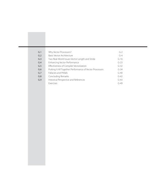
G.1<br />
G.2<br />
G.3<br />
G.4<br />
G.5<br />
G.6<br />
G.7<br />
G.8<br />
G.9<br />
Why <strong>Vector</strong> <strong>Processors</strong>? G-2<br />
Basic <strong>Vector</strong> Architecture G-4<br />
Two Real-World Issues: <strong>Vector</strong> Length and Stride G-16<br />
Enhancing <strong>Vector</strong> Performance G-23<br />
Effectiveness of Compiler <strong>Vector</strong>ization G-32<br />
Putting It All Together: Performance of <strong>Vector</strong> <strong>Processors</strong> G-34<br />
Fallacies and Pitfalls G-40<br />
Concluding Remarks G-42<br />
Historical Perspective and References G-43<br />
Exercises G-49
G<br />
<strong>Vector</strong> <strong>Processors</strong><br />
<strong>Revised</strong> <strong>by</strong> <strong>Krste</strong> <strong>Asanovic</strong><br />
Department of Electrical Engineering and Computer Science, MIT<br />
I’m certainly not inventing vector processors. There are three kinds<br />
that I know of existing today. They are represented <strong>by</strong> the Illiac-IV, the<br />
(CDC) Star processor, and the TI (ASC) processor. Those three were all<br />
pioneering processors. . . . One of the problems of being a pioneer is<br />
you always make mistakes and I never, never want to be a pioneer. It’s<br />
always best to come second when you can look at the mistakes the<br />
pioneers made.<br />
Seymour Cray<br />
Public lecture at Lawrence Livermore Laboratories<br />
on the introduction of the Cray-1 (1976)<br />
© 2003 Elsevier Science (USA). All rights reserved.
G-2<br />
■<br />
<strong>Appendix</strong> G<br />
<strong>Vector</strong> <strong>Processors</strong><br />
G.1 Why <strong>Vector</strong> <strong>Processors</strong>?<br />
In Chapters 3 and 4 we saw how we could significantly increase the performance<br />
of a processor <strong>by</strong> issuing multiple instructions per clock cycle and <strong>by</strong> more<br />
deeply pipelining the execution units to allow greater exploitation of instructionlevel<br />
parallelism. (This appendix assumes that you have read Chapters 3 and 4<br />
completely; in addition, the discussion on vector memory systems assumes that<br />
you have read Chapter 5.) Unfortunately, we also saw that there are serious difficulties<br />
in exploiting ever larger degrees of ILP.<br />
As we increase both the width of instruction issue and the depth of the<br />
machine pipelines, we also increase the number of independent instructions<br />
required to keep the processor busy with useful work. This means an increase in<br />
the number of partially executed instructions that can be in flight at one time. For<br />
a dynamically-scheduled machine, hardware structures, such as instruction windows,<br />
reorder buffers, and rename register files, must grow to have sufficient<br />
capacity to hold all in-flight instructions, and worse, the number of ports on each<br />
element of these structures must grow with the issue width. The logic to track<br />
dependencies between all in-flight instructions grows quadratically in the number<br />
of instructions. Even a statically scheduled VLIW machine, which shifts more of<br />
the scheduling burden to the compiler, requires more registers, more ports per<br />
register, and more hazard interlock logic (assuming a design where hardware<br />
manages interlocks after issue time) to support more in-flight instructions, which<br />
similarly cause quadratic increases in circuit size and complexity. This rapid<br />
increase in circuit complexity makes it difficult to build machines that can control<br />
large numbers of in-flight instructions, and hence limits practical issue widths<br />
and pipeline depths.<br />
<strong>Vector</strong> processors were successfully commercialized long before instructionlevel<br />
parallel machines and take an alternative approach to controlling multiple<br />
functional units with deep pipelines. <strong>Vector</strong> processors provide high-level operations<br />
that work on vectors—<br />
linear arrays of numbers. A typical vector operation<br />
might add two 64-element, floating-point vectors to obtain a single 64-element<br />
vector result. The vector instruction is equivalent to an entire loop, with each iteration<br />
computing one of the 64 elements of the result, updating the indices, and<br />
branching back to the beginning.<br />
<strong>Vector</strong> instructions have several important properties that solve most of the<br />
problems mentioned above:<br />
■<br />
■<br />
A single vector instruction specifies a great deal of work—it is equivalent to<br />
executing an entire loop. Each instruction represents tens or hundreds of<br />
operations, and so the instruction fetch and decode bandwidth needed to keep<br />
multiple deeply pipelined functional units busy is dramatically reduced.<br />
By using a vector instruction, the compiler or programmer indicates that the<br />
computation of each result in the vector is independent of the computation of<br />
other results in the same vector and so hardware does not have to check for<br />
data hazards within a vector instruction. The elements in the vector can be
■<br />
■<br />
■<br />
G.1 Why <strong>Vector</strong> <strong>Processors</strong>?<br />
■<br />
G-3<br />
computed using an array of parallel functional units, or a single very deeply<br />
pipelined functional unit, or any intermediate configuration of parallel and<br />
pipelined functional units.<br />
Hardware need only check for data hazards between two vector instructions<br />
once per vector operand, not once for every element within the vectors. That<br />
means the dependency checking logic required between two vector instructions<br />
is approximately the same as that required between two scalar instructions, but<br />
now many more elemental operations can be in flight for the same complexity<br />
of control logic.<br />
<strong>Vector</strong> instructions that access memory have a known access pattern. If the<br />
vector’s elements are all adjacent, then fetching the vector from a set of<br />
heavily interleaved memory banks works very well (as we saw in Section<br />
5.8). The high latency of initiating a main memory access versus accessing a<br />
cache is amortized, because a single access is initiated for the entire vector<br />
rather than to a single word. Thus, the cost of the latency to main memory is<br />
seen only once for the entire vector, rather than once for each word of the<br />
vector.<br />
Because an entire loop is replaced <strong>by</strong> a vector instruction whose behavior is<br />
predetermined, control hazards that would normally arise from the loop<br />
branch are nonexistent.<br />
For these reasons, vector operations can be made faster than a sequence of scalar<br />
operations on the same number of data items, and designers are motivated to<br />
include vector units if the application domain can use them frequently.<br />
As mentioned above, vector processors pipeline and parallelize the operations<br />
on the individual elements of a vector. The operations include not only the arithmetic<br />
operations (multiplication, addition, and so on), but also memory accesses<br />
and effective address calculations. In addition, most high-end vector processors<br />
allow multiple vector instructions to be in progress at the same time, creating further<br />
parallelism among the operations on different vectors.<br />
<strong>Vector</strong> processors are particularly useful for large scientific and engineering<br />
applications, including car crash simulations and weather forecasting, for which a<br />
typical job might take dozens of hours of supercomputer time running over multigiga<strong>by</strong>te<br />
data sets. Multimedia applications can also benefit from vector processing,<br />
as they contain abundant data parallelism and process large data streams. A<br />
high-speed pipelined processor will usually use a cache to avoid forcing memory<br />
reference instructions to have very long latency. Unfortunately, big, long-running,<br />
scientific programs often have very large active data sets that are sometimes<br />
accessed with low locality, yielding poor performance from the memory hierarchy.<br />
This problem could be overcome <strong>by</strong> not caching these structures if it were<br />
possible to determine the memory access patterns and pipeline the memory<br />
accesses efficiently. Novel cache architectures and compiler assistance through<br />
blocking and prefetching are decreasing these memory hierarchy problems, but<br />
they continue to be serious in some applications.
G-4<br />
■<br />
<strong>Appendix</strong> G<br />
<strong>Vector</strong> <strong>Processors</strong><br />
G.2 Basic <strong>Vector</strong> Architecture<br />
A vector processor typically consists of an ordinary pipelined scalar unit plus a<br />
vector unit. All functional units within the vector unit have a latency of several<br />
clock cycles. This allows a shorter clock cycle time and is compatible with longrunning<br />
vector operations that can be deeply pipelined without generating hazards.<br />
Most vector processors allow the vectors to be dealt with as floating-point<br />
numbers, as integers, or as logical data. Here we will focus on floating point. The<br />
scalar unit is basically no different from the type of advanced pipelined CPU discussed<br />
in Chapters 3 and 4, and commercial vector machines have included both<br />
out-of-order scalar units (NEC SX/5) and VLIW scalar units (Fujitsu VPP5000).<br />
There are two primary types of architectures for vector processors: vectorregister<br />
processors and memory-memory vector processors.<br />
In a vector-register<br />
processor, all vector operations—except load and store—are among the vector<br />
registers. These architectures are the vector counterpart of a load-store architecture.<br />
All major vector computers shipped since the late 1980s use a vector-register<br />
architecture, including the Cray Research processors (Cray-1, Cray-2, X-MP, Y-<br />
MP, C90, T90, and SV1), the Japanese supercomputers (NEC SX/2 through SX/5,<br />
Fujitsu VP200 through VPP5000, and the Hitachi S820 and S-8300), and the minisupercomputers<br />
(Convex C-1 through C-4). In a memory-memory vector processor,<br />
all vector operations are memory to memory. The first vector computers were<br />
of this type, as were CDC’s vector computers. From this point on we will focus on<br />
vector-register architectures only; we will briefly return to memory-memory vector<br />
architectures at the end of the appendix (Section G.9) to discuss why they have<br />
not been as successful as vector-register architectures.<br />
We begin with a vector-register processor consisting of the primary components<br />
shown in Figure G.1. This processor, which is loosely based on the Cray-<br />
1, is the foundation for discussion throughout most of this appendix. We will call<br />
it VMIPS; its scalar portion is MIPS, and its vector portion is the logical vector<br />
extension of MIPS. The rest of this section examines how the basic architecture<br />
of VMIPS relates to other processors.<br />
The primary components of the instruction set architecture of VMIPS are the<br />
following:<br />
■<br />
<strong>Vector</strong> registers—Each<br />
vector register is a fixed-length bank holding a single<br />
vector. VMIPS has eight vector registers, and each vector register holds 64<br />
elements. Each vector register must have at least two read ports and one write<br />
port in VMIPS. This will allow a high degree of overlap among vector operations<br />
to different vector registers. (We do not consider the problem of a shortage<br />
of vector-register ports. In real machines this would result in a structural<br />
hazard.) The read and write ports, which total at least 16 read ports and 8<br />
write ports, are connected to the functional unit inputs or outputs <strong>by</strong> a pair of<br />
crossbars. (The description of the vector-register file design has been simplified<br />
here. Real machines make use of the regular access pattern within a vector<br />
instruction to reduce the costs of the vector-register file circuitry<br />
[<strong>Asanovic</strong> 1998]. For example, the Cray-1 manages to implement the register<br />
file with only a single port per register.)
■<br />
■<br />
G.2 Basic <strong>Vector</strong> Architecture<br />
■<br />
G-5<br />
<strong>Vector</strong> functional units—Each<br />
unit is fully pipelined and can start a new operation<br />
on every clock cycle. A control unit is needed to detect hazards, both<br />
from conflicts for the functional units (structural hazards) and from conflicts<br />
for register accesses (data hazards). VMIPS has five functional units, as shown<br />
in Figure G.1. For simplicity, we will focus exclusively on the floating-point<br />
functional units. Depending on the vector processor, scalar operations either<br />
use the vector functional units or use a dedicated set. We assume the functional<br />
units are shared, but again, for simplicity, we ignore potential conflicts.<br />
<strong>Vector</strong> load-store unit—This<br />
is a vector memory unit that loads or stores a<br />
vector to or from memory. The VMIPS vector loads and stores are fully pipelined,<br />
so that words can be moved between the vector registers and memory<br />
<strong>Vector</strong><br />
registers<br />
Main memory<br />
<strong>Vector</strong><br />
load-store<br />
Scalar<br />
registers<br />
FP add/subtract<br />
FP multiply<br />
FP divide<br />
Integer<br />
Logical<br />
Figure G.1 The basic structure of a vector-register architecture, VMIPS. This processor<br />
has a scalar architecture just like MIPS. There are also eight 64-element vector registers,<br />
and all the functional units are vector functional units. Special vector instructions<br />
are defined both for arithmetic and for memory accesses. We show vector units for logical<br />
and integer operations. These are included so that VMIPS looks like a standard vector<br />
processor, which usually includes these units. However, we will not be discussing<br />
these units except in the exercises. The vector and scalar registers have a significant<br />
number of read and write ports to allow multiple simultaneous vector operations.<br />
These ports are connected to the inputs and outputs of the vector functional units <strong>by</strong> a<br />
set of crossbars (shown in thick gray lines). In Section G.4 we add chaining, which will<br />
require additional interconnect capability.
G-6<br />
■<br />
<strong>Appendix</strong> G<br />
<strong>Vector</strong> <strong>Processors</strong><br />
■<br />
with a bandwidth of 1 word per clock cycle, after an initial latency. This unit<br />
would also normally handle scalar loads and stores.<br />
A set of scalar registers—Scalar<br />
registers can also provide data as input to the<br />
vector functional units, as well as compute addresses to pass to the vector<br />
load-store unit. These are the normal 32 general-purpose registers and 32<br />
floating-point registers of MIPS. Scalar values are read out of the scalar register<br />
file, then latched at one input of the vector functional units.<br />
Figure G.2 shows the characteristics of some typical vector processors,<br />
including the size and count of the registers, the number and types of functional<br />
units, and the number of load-store units. The last column in Figure G.2 shows<br />
the number of lanes in the machine, which is the number of parallel pipelines<br />
used to execute operations within each vector instruction. Lanes are described<br />
later in Section G.4; here we assume VMIPS has only a single pipeline per vector<br />
functional unit (one lane).<br />
In VMIPS, vector operations use the same names as MIPS operations, but<br />
with the letter “V” appended. Thus, ADDV.D is an add of two double-precision<br />
vectors. The vector instructions take as their input either a pair of vector registers<br />
(ADDV.D) or a vector register and a scalar register, designated <strong>by</strong> appending “VS”<br />
(ADDVS.D). In the latter case, the value in the scalar register is used as the input<br />
for all operations—the operation ADDVS.D will add the contents of a scalar register<br />
to each element in a vector register. The scalar value is copied over to the vector<br />
functional unit at issue time. Most vector operations have a vector destination<br />
register, although a few (population count) produce a scalar value, which is stored<br />
to a scalar register. The names LV and SV denote vector load and vector store, and<br />
they load or store an entire vector of double-precision data. One operand is<br />
the vector register to be loaded or stored; the other operand, which is a MIPS<br />
general-purpose register, is the starting address of the vector in memory.<br />
Figure G.3 lists the VMIPS vector instructions. In addition to the vector registers,<br />
we need two additional special-purpose registers: the vector-length and vectormask<br />
registers. We will discuss these registers and their purpose in Sections G.3<br />
and G.4, respectively.<br />
How <strong>Vector</strong> <strong>Processors</strong> Work: An Example<br />
A vector processor is best understood <strong>by</strong> looking at a vector loop on VMIPS.<br />
Let’s take a typical vector problem, which will be used throughout this appendix:<br />
Y = a ×<br />
X + Y<br />
X and Y are vectors, initially resident in memory, and a is a scalar. This is the socalled<br />
SAXPY or DAXPY loop that forms the inner loop of the Linpack benchmark.<br />
(SAXPY stands for single-precision a × X plus Y; DAXPY for doubleprecision<br />
a × X plus Y.) Linpack is a collection of linear algebra routines, and the<br />
routines for performing Gaussian elimination constitute what is known as the
Processor (year)<br />
Clock<br />
rate<br />
(MHz)<br />
<strong>Vector</strong><br />
registers<br />
Elements per<br />
register<br />
(64-bit<br />
elements) <strong>Vector</strong> arithmetic units<br />
G.2 Basic <strong>Vector</strong> Architecture<br />
Cray-1 (1976) 80 8 64 6: FP add, FP multiply, FP reciprocal,<br />
integer add, logical, shift<br />
Cray X-MP<br />
(1983)<br />
Cray Y-MP (1988)<br />
118<br />
166<br />
8 64<br />
8: FP add, FP multiply, FP reciprocal,<br />
integer add, 2 logical, shift, population<br />
count/parity<br />
Cray-2 (1985) 244 8 64 5: FP add, FP multiply, FP reciprocal/<br />
sqrt, integer add/shift/population<br />
count, logical<br />
Fujitsu VP100/<br />
VP200 (1982)<br />
Hitachi S810/<br />
S820 (1983)<br />
Convex C-1<br />
(1985)<br />
133 8–256 32–1024 3: FP or integer add/logical, multiply,<br />
divide<br />
71 32 256 4: FP multiply-add, FP multiply/<br />
divide-add unit, 2 integer add/logical<br />
10 8 128 2: FP or integer multiply/divide, add/<br />
logical<br />
NEC SX/2 (1985) 167 8 + 32 256 4: FP multiply/divide, FP add, integer<br />
add/logical, shift<br />
Cray C90 (1991)<br />
Cray T90 (1995)<br />
240<br />
460<br />
8 128<br />
8: FP add, FP multiply, FP reciprocal,<br />
integer add, 2 logical, shift, population<br />
count/parity<br />
NEC SX/5 (1998) 312 8 + 64 512 4: FP or integer add/shift, multiply,<br />
divide, logical<br />
Fujitsu VPP5000<br />
(1999)<br />
Cray SV1 (1998)<br />
SV1ex (2001)<br />
300 8–256 128–4096 3: FP or integer multiply, add/logical,<br />
divide<br />
300<br />
500<br />
8 64<br />
8: FP add, FP multiply, FP reciprocal,<br />
integer add, 2 logical, shift, population<br />
count/parity<br />
VMIPS (2001) 500 8 64 5: FP multiply, FP divide, FP add,<br />
integer add/shift, logical<br />
■<br />
<strong>Vector</strong><br />
load-store<br />
units Lanes<br />
1 1<br />
2 loads<br />
1 store<br />
1<br />
1 1<br />
G-7<br />
2 1 (VP100)<br />
2 (VP200)<br />
3 loads<br />
1 store<br />
1 (S810)<br />
2 (S820)<br />
1 1 (64 bit)<br />
2 (32 bit)<br />
1 4<br />
2 loads<br />
1 store<br />
2<br />
1 16<br />
1 load<br />
1 store<br />
1 load-store<br />
1 load<br />
16<br />
2<br />
8 (MSP)<br />
1 load-store 1<br />
Figure G.2 Characteristics of several vector-register architectures. If the machine is a multiprocessor, the entries<br />
correspond to the characteristics of one processor. Several of the machines have different clock rates in the vector<br />
and scalar units; the clock rates shown are for the vector units. The Fujitsu machines’ vector registers are configurable:<br />
The size and count of the 8K 64-bit entries may be varied inversely to one another (e.g., on the VP200, from<br />
eight registers each 1K elements long to 256 registers each 32 elements long). The NEC machines have eight foreground<br />
vector registers connected to the arithmetic units plus 32–64 background vector registers connected<br />
between the memory system and the foreground vector registers. The reciprocal unit on the Cray processors is used<br />
to do division (and square root on the Cray-2). Add pipelines perform add and subtract. The multiply/divide-add unit<br />
on the Hitachi S810/820 performs an FP multiply or divide followed <strong>by</strong> an add or subtract (while the multiply-add<br />
unit performs a multiply followed <strong>by</strong> an add or subtract). Note that most processors use the vector FP multiply and<br />
divide units for vector integer multiply and divide, and several of the processors use the same units for FP scalar and<br />
FP vector operations. Each vector load-store unit represents the ability to do an independent, overlapped transfer to<br />
or from the vector registers. The number of lanes is the number of parallel pipelines in each of the functional units as<br />
described in Section G.4. For example, the NEC SX/5 can complete 16 multiplies per cycle in the multiply functional<br />
unit. The Convex C-1 can split its single 64-bit lane into two 32-bit lanes to increase performance for applications that<br />
require only reduced precision. The Cray SV1 can group four CPUs with two lanes each to act in unison as a single<br />
larger CPU with eight lanes, which Cray calls a Multi-Streaming Processor (MSP).
G-8<br />
■<br />
<strong>Appendix</strong> G<br />
<strong>Vector</strong> <strong>Processors</strong><br />
Instruction Operands Function<br />
ADDV.D<br />
ADDVS.D<br />
SUBV.D<br />
SUBVS.D<br />
SUBSV.D<br />
MULV.D<br />
MULVS.D<br />
DIVV.D<br />
DIVVS.D<br />
DIVSV.D<br />
V1,V2,V3<br />
V1,V2,F0<br />
V1,V2,V3<br />
V1,V2,F0<br />
V1,F0,V2<br />
V1,V2,V3<br />
V1,V2,F0<br />
V1,V2,V3<br />
V1,V2,F0<br />
V1,F0,V2<br />
Add elements of V2 and V3,<br />
then put each result in V1.<br />
Add F0 to each element of V2,<br />
then put each result in V1.<br />
Subtract elements of V3 from V2,<br />
then put each result in V1.<br />
Subtract F0 from elements of V2,<br />
then put each result in V1.<br />
Subtract elements of V2 from F0,<br />
then put each result in V1.<br />
Multiply elements of V2 and V3,<br />
then put each result in V1.<br />
Multiply each element of V2 <strong>by</strong> F0,<br />
then put each result in<br />
Divide elements of V2 <strong>by</strong> V3, then put each result in V1.<br />
Divide elements of V2 <strong>by</strong> F0, then put each result in V1.<br />
Divide F0 <strong>by</strong> elements of V2, then put each result in V1.<br />
LV V1,R1 Load vector register V1 from memory starting at address R1.<br />
SV R1,V1 Store vector register V1 into memory starting at address R1.<br />
LVWS V1,(R1,R2) Load V1 from address at R1 with stride in R2, i.e., R1+i × R2.<br />
SVWS (R1,R2),V1 Store V1 from address at R1 with stride in R2, i.e., R1+i × R2.<br />
LVI V1,(R1+V2) Load V1 with vector whose elements are at R1+V2(i), i.e., V2 is an index.<br />
SVI (R1+V2),V1 Store V1 to vector whose elements are at R1+V2(i), i.e., V2 is an index.<br />
CVI V1,R1 Create an index vector <strong>by</strong> storing the values 0, 1 × R1, 2 × R1,...,63 × R1 into V1.<br />
S--V.D V1,V2 Compare the elements (EQ, NE, GT, LT, GE, LE) in V1 and V2. If condition is true, put<br />
S--VS.D V1,F0 a 1 in the corresponding bit vector; otherwise put 0. Put resulting bit vector in vectormask<br />
register (VM). The instruction S--VS.D performs the same compare but using a<br />
scalar value as one operand.<br />
POP R1,VM Count the 1s in the vector-mask register and store count in R1.<br />
CVM Set the vector-mask register to all 1s.<br />
MTC1 VLR,R1 Move contents of R1 to the vector-length register.<br />
MFC1 R1,VLR Move the contents of the vector-length register to R1.<br />
MVTM VM,F0 Move contents of F0 to the vector-mask register.<br />
MVFM F0,VM Move contents of vector-mask register to F0.<br />
Figure G.3 The VMIPS vector instructions. Only the double-precision FP operations are shown. In addition to the<br />
vector registers, there are two special registers, VLR (discussed in Section G.3) and VM (discussed in Section G.4).<br />
These special registers are assumed to live in the MIPS coprocessor 1 space along with the FPU registers. The operations<br />
with stride are explained in Section G.3, and the use of the index creation and indexed load-store operations<br />
are explained in Section G.4.<br />
Linpack benchmark. The DAXPY routine, which implements the preceding loop,<br />
represents a small fraction of the source code of the Linpack benchmark, but it<br />
accounts for most of the execution time for the benchmark.<br />
For now, let us assume that the number of elements, or length, of a vector register<br />
(64) matches the length of the vector operation we are interested in. (This<br />
restriction will be lifted shortly.)<br />
V1.
G.2 Basic <strong>Vector</strong> Architecture ■ G-9<br />
Example Show the code for MIPS and VMIPS for the DAXPY loop. Assume that the starting<br />
addresses of X and Y are in Rx and Ry, respectively.<br />
Answer Here is the MIPS code.<br />
L.D F0,a ;load scalar a<br />
DADDIU R4,Rx,#512 ;last address to load<br />
Loop: L.D F2,0(Rx) ;load X(i)<br />
MUL.D F2,F2,F0 ;a × X(i)<br />
L.D F4,0(Ry) ;load Y(i)<br />
ADD.D F4,F4,F2 ;a ×<br />
X(i) + Y(i)<br />
S.D 0(Ry),F4 ;store into Y(i)<br />
DADDIU Rx,Rx,#8 ;increment index to X<br />
DADDIU Ry,Ry,#8 ;increment index to Y<br />
DSUBU R20,R4,Rx ;compute bound<br />
BNEZ R20,Loop ;check if done<br />
Here is the VMIPS code for DAXPY.<br />
L.D F0,a ;load scalar a<br />
LV V1,Rx ;load vector X<br />
MULVS.D V2,V1,F0 ;vector-scalar multiply<br />
LV V3,Ry ;load vector Y<br />
ADDV.D V4,V2,V3 ;add<br />
SV Ry,V4 ;store the result<br />
There are some interesting comparisons between the two code segments in this<br />
example. The most dramatic is that the vector processor greatly reduces the<br />
dynamic instruction bandwidth, executing only six instructions versus almost 600<br />
for MIPS. This reduction occurs both because the vector operations work on 64<br />
elements and because the overhead instructions that constitute nearly half the<br />
loop on MIPS are not present in the VMIPS code.<br />
Another important difference is the frequency of pipeline interlocks. In the<br />
straightforward MIPS code every ADD.D must wait for a MUL.D, and every S.D<br />
must wait for the ADD.D. On the vector processor, each vector instruction will<br />
only stall for the first element in each vector, and then subsequent elements will<br />
flow smoothly down the pipeline. Thus, pipeline stalls are required only once per<br />
vector operation, rather than once per vector element. In this example, the<br />
pipeline stall frequency on MIPS will be about 64 times higher than it is on<br />
VMIPS. The pipeline stalls can be eliminated on MIPS <strong>by</strong> using software pipelining<br />
or loop unrolling (as we saw in Chapter 4). However, the large difference in<br />
instruction bandwidth cannot be reduced.
G-10 ■ <strong>Appendix</strong> G <strong>Vector</strong> <strong>Processors</strong><br />
<strong>Vector</strong> Execution Time<br />
The execution time of a sequence of vector operations primarily depends on three<br />
factors: the length of the operand vectors, structural hazards among the operations,<br />
and the data dependences. Given the vector length and the initiation rate,<br />
which is the rate at which a vector unit consumes new operands and produces<br />
new results, we can compute the time for a single vector instruction. All modern<br />
supercomputers have vector functional units with multiple parallel pipelines (or<br />
lanes) that can produce two or more results per clock cycle, but may also have<br />
some functional units that are not fully pipelined. For simplicity, our VMIPS<br />
implementation has one lane with an initiation rate of one element per clock<br />
cycle for individual operations. Thus, the execution time for a single vector<br />
instruction is approximately the vector length.<br />
To simplify the discussion of vector execution and its timing, we will use the<br />
notion of a convoy, which is the set of vector instructions that could potentially<br />
begin execution together in one clock period. (Although the concept of a convoy<br />
is used in vector compilers, no standard terminology exists. Hence, we created<br />
the term convoy.) The instructions in a convoy must not contain any structural or<br />
data hazards (though we will relax this later); if such hazards were present, the<br />
instructions in the potential convoy would need to be serialized and initiated in<br />
different convoys. Placing vector instructions into a convoy is analogous to placing<br />
scalar operations into a VLIW instruction. To keep the analysis simple, we<br />
assume that a convoy of instructions must complete execution before any other<br />
instructions (scalar or vector) can begin execution. We will relax this in Section<br />
G.4 <strong>by</strong> using a less restrictive, but more complex, method for issuing instructions.<br />
Accompanying the notion of a convoy is a timing metric, called a chime, that<br />
can be used for estimating the performance of a vector sequence consisting of<br />
convoys. A chime is the unit of time taken to execute one convoy. A chime is an<br />
approximate measure of execution time for a vector sequence; a chime measurement<br />
is independent of vector length. Thus, a vector sequence that consists of m<br />
convoys executes in m chimes, and for a vector length of n, this is approximately<br />
m × n clock cycles. A chime approximation ignores some processor-specific overheads,<br />
many of which are dependent on vector length. Hence, measuring time in<br />
chimes is a better approximation for long vectors. We will use the chime measurement,<br />
rather than clock cycles per result, to explicitly indicate that certain<br />
overheads are being ignored.<br />
If we know the number of convoys in a vector sequence, we know the execution<br />
time in chimes. One source of overhead ignored in measuring chimes is any<br />
limitation on initiating multiple vector instructions in a clock cycle. If only one<br />
vector instruction can be initiated in a clock cycle (the reality in most vector<br />
processors), the chime count will underestimate the actual execution time of a<br />
convoy. Because the vector length is typically much greater than the number of<br />
instructions in the convoy, we will simply assume that the convoy executes in one<br />
chime.
G.2 Basic <strong>Vector</strong> Architecture ■ G-11<br />
Example Show how the following code sequence lays out in convoys, assuming a single<br />
copy of each vector functional unit:<br />
LV V1,Rx ;load vector X<br />
MULVS.D V2,V1,F0 ;vector-scalar multiply<br />
LV V3,Ry ;load vector Y<br />
ADDV.D V4,V2,V3 ;add<br />
SV Ry,V4 ;store the result<br />
How many chimes will this vector sequence take? How many cycles per FLOP<br />
(floating-point operation) are needed ignoring vector instruction issue overhead?<br />
Answer The first convoy is occupied <strong>by</strong> the first LV instruction. The MULVS.D is dependent<br />
on the first LV, so it cannot be in the same convoy. The second LV instruction can<br />
be in the same convoy as the MULVS.D. The ADDV.D is dependent on the second<br />
LV, so it must come in yet a third convoy, and finally the SV depends on the<br />
ADDV.D, so it must go in a following convoy. This leads to the following layout of<br />
vector instructions into convoys:<br />
1. LV<br />
2. MULVS.D LV<br />
3. ADDV.D<br />
4. SV<br />
The sequence requires four convoys and hence takes four chimes. Since the<br />
sequence takes a total of four chimes and there are two floating-point operations<br />
per result, the number of cycles per FLOP is 2 (ignoring any vector instruction<br />
issue overhead). Note that although we allow the MULVS.D and the LV both to execute<br />
in convoy 2, most vector machines will take 2 clock cycles to initiate the<br />
instructions.<br />
The chime approximation is reasonably accurate for long vectors. For example,<br />
for 64-element vectors, the time in chimes is four, so the sequence would<br />
take about 256 clock cycles. The overhead of issuing convoy 2 in two separate<br />
clocks would be small.<br />
Another source of overhead is far more significant than the issue limitation.<br />
The most important source of overhead ignored <strong>by</strong> the chime model is vector<br />
start-up time. The start-up time comes from the pipelining latency of the vector<br />
operation and is principally determined <strong>by</strong> how deep the pipeline is for the functional<br />
unit used. The start-up time increases the effective time to execute a convoy<br />
to more than one chime. Because of our assumption that convoys do not<br />
overlap in time, the start-up time delays the execution of subsequent convoys. Of<br />
course the instructions in successive convoys have either structural conflicts for<br />
some functional unit or are data dependent, so the assumption of no overlap is
G-12 ■ <strong>Appendix</strong> G <strong>Vector</strong> <strong>Processors</strong><br />
reasonable. The actual time to complete a convoy is determined <strong>by</strong> the sum of the<br />
vector length and the start-up time. If vector lengths were infinite, this start-up<br />
overhead would be amortized, but finite vector lengths expose it, as the following<br />
example shows.<br />
Example Assume the start-up overhead for functional units is shown in Figure G.4.<br />
Show the time that each convoy can begin and the total number of cycles needed.<br />
How does the time compare to the chime approximation for a vector of length<br />
64?<br />
Answer Figure G.5 provides the answer in convoys, assuming that the vector length is n.<br />
One tricky question is when we assume the vector sequence is done; this determines<br />
whether the start-up time of the SV is visible or not. We assume that the<br />
instructions following cannot fit in the same convoy, and we have already<br />
assumed that convoys do not overlap. Thus the total time is given <strong>by</strong> the time<br />
until the last vector instruction in the last convoy completes. This is an approximation,<br />
and the start-up time of the last vector instruction may be seen in some<br />
sequences and not in others. For simplicity, we always include it.<br />
The time per result for a vector of length 64 is 4 + (42/64) = 4.65 clock<br />
cycles, while the chime approximation would be 4. The execution time with startup<br />
overhead is 1.16 times higher.<br />
Unit Start-up overhead (cycles)<br />
Load and store unit 12<br />
Multiply unit 7<br />
Add unit 6<br />
Figure G.4 Start-up overhead.<br />
Convoy Starting time First-result time Last-result time<br />
1. LV 0 12 11 + n<br />
2. MULVS.D LV 12 + n 12 + n + 12 23 + 2n<br />
3. ADDV.D 24 + 2n 24 + 2n + 6 29 + 3n<br />
4. SV 30 + 3n 30 + 3n + 12 41 + 4n<br />
Figure G.5 Starting times and first- and last-result times for convoys 1 through 4.<br />
The vector length is n.
G.2 Basic <strong>Vector</strong> Architecture ■ G-13<br />
For simplicity, we will use the chime approximation for running time, incorporating<br />
start-up time effects only when we want more detailed performance or to<br />
illustrate the benefits of some enhancement. For long vectors, a typical situation,<br />
the overhead effect is not that large. Later in the appendix we will explore ways<br />
to reduce start-up overhead.<br />
Start-up time for an instruction comes from the pipeline depth for the functional<br />
unit implementing that instruction. If the initiation rate is to be kept at 1<br />
clock cycle per result, then<br />
Pipeline depth =<br />
Total functional unit time<br />
------------------------------------------------------------<br />
Clock cycle time<br />
For example, if an operation takes 10 clock cycles, it must be pipelined 10 deep<br />
to achieve an initiation rate of one per clock cycle. Pipeline depth, then, is determined<br />
<strong>by</strong> the complexity of the operation and the clock cycle time of the processor.<br />
The pipeline depths of functional units vary widely—from 2 to 20 stages is<br />
not uncommon—although the most heavily used units have pipeline depths of 4–<br />
8 clock cycles.<br />
For VMIPS, we will use the same pipeline depths as the Cray-1, although<br />
latencies in more modern processors have tended to increase, especially for loads.<br />
All functional units are fully pipelined. As shown in Figure G.6, pipeline depths<br />
are 6 clock cycles for floating-point add and 7 clock cycles for floating-point multiply.<br />
On VMIPS, as on most vector processors, independent vector operations<br />
using different functional units can issue in the same convoy.<br />
<strong>Vector</strong> Load-Store Units and <strong>Vector</strong> Memory Systems<br />
The behavior of the load-store vector unit is significantly more complicated than<br />
that of the arithmetic functional units. The start-up time for a load is the time to<br />
get the first word from memory into a register. If the rest of the vector can be supplied<br />
without stalling, then the vector initiation rate is equal to the rate at which<br />
new words are fetched or stored. Unlike simpler functional units, the initiation<br />
rate may not necessarily be 1 clock cycle because memory bank stalls can reduce<br />
effective throughput.<br />
Operation Start-up penalty<br />
<strong>Vector</strong> add 6<br />
<strong>Vector</strong> multiply 7<br />
<strong>Vector</strong> divide 20<br />
<strong>Vector</strong> load 12<br />
Figure G.6 Start-up penalties on VMIPS. These are the start-up penalties in clock<br />
cycles for VMIPS vector operations.
G-14 ■ <strong>Appendix</strong> G <strong>Vector</strong> <strong>Processors</strong><br />
Typically, penalties for start-ups on load-store units are higher than those for<br />
arithmetic functional units—over 100 clock cycles on some processors. For<br />
VMIPS we will assume a start-up time of 12 clock cycles, the same as the Cray-<br />
1. Figure G.6 summarizes the start-up penalties for VMIPS vector operations.<br />
To maintain an initiation rate of 1 word fetched or stored per clock, the memory<br />
system must be capable of producing or accepting this much data. This is<br />
usually done <strong>by</strong> creating multiple memory banks, as discussed in Section 5.8. As<br />
we will see in the next section, having significant numbers of banks is useful for<br />
dealing with vector loads or stores that access rows or columns of data.<br />
Most vector processors use memory banks rather than simple interleaving for<br />
three primary reasons:<br />
1. Many vector computers support multiple loads or stores per clock, and the<br />
memory bank cycle time is often several times larger than the CPU cycle<br />
time. To support multiple simultaneous accesses, the memory system needs to<br />
have multiple banks and be able to control the addresses to the banks independently.<br />
2. As we will see in the next section, many vector processors support the ability<br />
to load or store data words that are not sequential. In such cases, independent<br />
bank addressing, rather than interleaving, is required.<br />
3. Many vector computers support multiple processors sharing the same memory<br />
system, and so each processor will be generating its own independent<br />
stream of addresses.<br />
In combination, these features lead to a large number of independent memory<br />
banks, as shown <strong>by</strong> the following example.<br />
Example The Cray T90 has a CPU clock cycle of 2.167 ns and in its largest configuration<br />
(Cray T932) has 32 processors each capable of generating four loads and two<br />
stores per CPU clock cycle. The CPU clock cycle is 2.167 ns, while the cycle<br />
time of the SRAMs used in the memory system is 15 ns. Calculate the minimum<br />
number of memory banks required to allow all CPUs to run at full memory bandwidth.<br />
Answer The maximum number of memory references each cycle is 192 (32 CPUs times 6<br />
references per CPU). Each SRAM bank is busy for 15/2.167 = 6.92 clock cycles,<br />
which we round up to 7 CPU clock cycles. Therefore we require a minimum of<br />
192 × 7 = 1344 memory banks!<br />
The Cray T932 actually has 1024 memory banks, and so the early models<br />
could not sustain full bandwidth to all CPUs simultaneously. A subsequent memory<br />
upgrade replaced the 15 ns asynchronous SRAMs with pipelined synchronous<br />
SRAMs that more than halved the memory cycle time, there<strong>by</strong> providing<br />
sufficient bandwidth.
G.2 Basic <strong>Vector</strong> Architecture ■ G-15<br />
In Chapter 5 we saw that the desired access rate and the bank access time<br />
determined how many banks were needed to access a memory without a stall.<br />
The next example shows how these timings work out in a vector processor.<br />
Example Suppose we want to fetch a vector of 64 elements starting at <strong>by</strong>te address 136,<br />
and a memory access takes 6 clocks. How many memory banks must we have to<br />
support one fetch per clock cycle? With what addresses are the banks accessed?<br />
When will the various elements arrive at the CPU?<br />
Answer Six clocks per access require at least six banks, but because we want the number<br />
of banks to be a power of two, we choose to have eight banks. Figure G.7 shows<br />
the timing for the first few sets of accesses for an eight-bank system with a 6clock-cycle<br />
access latency.<br />
Bank<br />
Cycle no. 0 1 2 3 4 5 6 7<br />
0 136<br />
1 busy 144<br />
2 busy busy 152<br />
3 busy busy busy 160<br />
4 busy busy busy busy 168<br />
5 busy busy busy busy busy 176<br />
6 busy busy busy busy busy 184<br />
7 192 busy busy busy busy busy<br />
8 busy 200 busy busy busy busy<br />
9 busy busy 208 busy busy busy<br />
10 busy busy busy 216 busy busy<br />
11 busy busy busy busy 224 busy<br />
12 busy busy busy busy busy 232<br />
13 busy busy busy busy busy 240<br />
14 busy busy busy busy busy 248<br />
15 256 busy busy busy busy busy<br />
16 busy 264 busy busy busy busy<br />
Figure G.7 Memory addresses (in <strong>by</strong>tes) <strong>by</strong> bank number and time slot at which<br />
access begins. Each memory bank latches the element address at the start of an access<br />
and is then busy for 6 clock cycles before returning a value to the CPU. Note that the<br />
CPU cannot keep all eight banks busy all the time because it is limited to supplying one<br />
new address and receiving one data item each cycle.
G-16 ■ <strong>Appendix</strong> G <strong>Vector</strong> <strong>Processors</strong><br />
The timing of real memory banks is usually split into two different components,<br />
the access latency and the bank cycle time (or bank busy time). The access<br />
latency is the time from when the address arrives at the bank until the bank<br />
returns a data value, while the busy time is the time the bank is occupied with one<br />
request. The access latency adds to the start-up cost of fetching a vector from<br />
memory (the total memory latency also includes time to traverse the pipelined<br />
interconnection networks that transfer addresses and data between the CPU and<br />
memory banks). The bank busy time governs the effective bandwidth of a memory<br />
system because a processor cannot issue a second request to the same bank<br />
until the bank busy time has elapsed.<br />
For simple unpipelined SRAM banks as used in the previous examples, the<br />
access latency and busy time are approximately the same. For a pipelined SRAM<br />
bank, however, the access latency is larger than the busy time because each element<br />
access only occupies one stage in the memory bank pipeline. For a DRAM<br />
bank, the access latency is usually shorter than the busy time because a DRAM<br />
needs extra time to restore the read value after the destructive read operation. For<br />
memory systems that support multiple simultaneous vector accesses or allow<br />
nonsequential accesses in vector loads or stores, the number of memory banks<br />
should be larger than the minimum; otherwise, memory bank conflicts will exist.<br />
We explore this in more detail in the next section.<br />
G.3 Two Real-World Issues: <strong>Vector</strong> Length and Stride<br />
This section deals with two issues that arise in real programs: What do you do<br />
when the vector length in a program is not exactly 64? How do you deal with<br />
nonadjacent elements in vectors that reside in memory? First, let’s consider the<br />
issue of vector length.<br />
<strong>Vector</strong>-Length Control<br />
A vector-register processor has a natural vector length determined <strong>by</strong> the number<br />
of elements in each vector register. This length, which is 64 for VMIPS, is<br />
unlikely to match the real vector length in a program. Moreover, in a real program<br />
the length of a particular vector operation is often unknown at compile time. In<br />
fact, a single piece of code may require different vector lengths. For example,<br />
consider this code:<br />
do 10 i = 1,n<br />
10 Y(i) = a ∗ X(i) + Y(i)<br />
The size of all the vector operations depends on n, which may not even be known<br />
until run time! The value of n might also be a parameter to a procedure containing<br />
the above loop and therefore be subject to change during execution.
G.3 Two Real-World Issues: <strong>Vector</strong> Length and Stride ■ G-17<br />
The solution to these problems is to create a vector-length register (VLR).<br />
The VLR controls the length of any vector operation, including a vector load or<br />
store. The value in the VLR, however, cannot be greater than the length of the<br />
vector registers. This solves our problem as long as the real length is less than or<br />
equal to the maximum vector length (MVL) defined <strong>by</strong> the processor.<br />
What if the value of n is not known at compile time, and thus may be greater<br />
than MVL? To tackle the second problem where the vector is longer than the<br />
maximum length, a technique called strip mining is used. Strip mining is the generation<br />
of code such that each vector operation is done for a size less than or<br />
equal to the MVL. We could strip-mine the loop in the same manner that we<br />
unrolled loops in Chapter 4: create one loop that handles any number of iterations<br />
that is a multiple of MVL and another loop that handles any remaining iterations,<br />
which must be less than MVL. In practice, compilers usually create a single stripmined<br />
loop that is parameterized to handle both portions <strong>by</strong> changing the length.<br />
The strip-mined version of the DAXPY loop written in FORTRAN, the major<br />
language used for scientific applications, is shown with C-style comments:<br />
low = 1<br />
VL = (n mod MVL) /*find the odd-size piece*/<br />
do 1 j = 0,(n / MVL) /*outer loop*/<br />
do 10 i = low, low + VL - 1 /*runs for length VL*/<br />
Y(i) = a * X(i) + Y(i) /*main operation*/<br />
10 continue<br />
low = low + VL /*start of next vector*/<br />
VL = MVL /*reset the length to max*/<br />
1 continue<br />
The term n/MVL represents truncating integer division (which is what FOR-<br />
TRAN does) and is used throughout this section. The effect of this loop is to<br />
block the vector into segments that are then processed <strong>by</strong> the inner loop. The<br />
length of the first segment is (n mod MVL), and all subsequent segments are of<br />
length MVL. This is depicted in Figure G.8.<br />
Value of j 0 1 2 3 . . . . . .<br />
n/MVL<br />
Range of i<br />
1..m (m + 1)..<br />
m + MVL<br />
(m +<br />
MVL + 1)<br />
.. m + 2 *<br />
MVL<br />
(m + 2 *<br />
MVL + 1)<br />
.. m + 3 *<br />
MVL<br />
. . . . . . (n – MVL<br />
+ 1).. n<br />
Figure G.8 A vector of arbitrary length processed with strip mining. All blocks but<br />
the first are of length MVL, utilizing the full power of the vector processor. In this figure,<br />
the variable m is used for the expression (n mod MVL).
G-18 ■ <strong>Appendix</strong> G <strong>Vector</strong> <strong>Processors</strong><br />
The inner loop of the preceding code is vectorizable with length VL, which is<br />
equal to either (n mod MVL) or MVL. The VLR register must be set twice—once<br />
at each place where the variable VL in the code is assigned. With multiple vector<br />
operations executing in parallel, the hardware must copy the value of VLR to the<br />
vector functional unit when a vector operation issues, in case VLR is changed for<br />
a subsequent vector operation.<br />
Several vector ISAs have been developed that allow implementations to have<br />
different maximum vector-register lengths. For example, the IBM vector extension<br />
for the IBM 370 series mainframes supports an MVL of anywhere between<br />
8 and 512 elements. A “load vector count and update” (VLVCU) instruction is<br />
provided to control strip-mined loops. The VLVCU instruction has a single scalar<br />
register operand that specifies the desired vector length. The vector-length<br />
register is set to the minimum of the desired length and the maximum available<br />
vector length, and this value is also subtracted from the scalar register, setting<br />
the condition codes to indicate if the loop should be terminated. In this way,<br />
object code can be moved unchanged between two different implementations<br />
while making full use of the available vector-register length within each stripmined<br />
loop iteration.<br />
In addition to the start-up overhead, we need to account for the overhead of<br />
executing the strip-mined loop. This strip-mining overhead, which arises from the<br />
need to reinitiate the vector sequence and set the VLR, effectively adds to the<br />
vector start-up time, assuming that a convoy does not overlap with other instructions.<br />
If that overhead for a convoy is 10 cycles, then the effective overhead per<br />
64 elements increases <strong>by</strong> 10 cycles, or 0.15 cycles per element.<br />
There are two key factors that contribute to the running time of a strip-mined<br />
loop consisting of a sequence of convoys:<br />
1. The number of convoys in the loop, which determines the number of chimes.<br />
We use the notation Tchime for the execution time in chimes.<br />
2. The overhead for each strip-mined sequence of convoys. This overhead consists<br />
of the cost of executing the scalar code for strip-mining each block,<br />
Tloop , plus the vector start-up cost for each convoy, Tstart .<br />
There may also be a fixed overhead associated with setting up the vector<br />
sequence the first time. In recent vector processors this overhead has become<br />
quite small, so we ignore it.<br />
The components can be used to state the total running time for a vector<br />
sequence operating on a vector of length n, which we will call T n :<br />
Tn =<br />
n<br />
------------ × ( Tloop + Tstart) + n × Tchime<br />
MVL<br />
The values of T start , T loop , and T chime are compiler and processor dependent. The<br />
register allocation and scheduling of the instructions affect both what goes in a<br />
convoy and the start-up overhead of each convoy.
G.3 Two Real-World Issues: <strong>Vector</strong> Length and Stride ■ G-19<br />
For simplicity, we will use a constant value for T loop on VMIPS. Based on a<br />
variety of measurements of Cray-1 vector execution, the value chosen is 15 for<br />
T loop . At first glance, you might think that this value is too small. The overhead in<br />
each loop requires setting up the vector starting addresses and the strides, incrementing<br />
counters, and executing a loop branch. In practice, these scalar instructions<br />
can be totally or partially overlapped with the vector instructions,<br />
minimizing the time spent on these overhead functions. The value of T loop of<br />
course depends on the loop structure, but the dependence is slight compared with<br />
the connection between the vector code and the values of T chime and T start .<br />
Example What is the execution time on VMIPS for the vector operation A = B × s, where s<br />
is a scalar and the length of the vectors A and B is 200?<br />
Answer Assume the addresses of A and B are initially in Ra and Rb, s is in Fs, and recall<br />
that for MIPS (and VMIPS) R0 always holds 0. Since (200 mod 64) = 8, the first<br />
iteration of the strip-mined loop will execute for a vector length of 8 elements,<br />
and the following iterations will execute for a vector length of 64 elements. The<br />
starting <strong>by</strong>te addresses of the next segment of each vector is eight times the vector<br />
length. Since the vector length is either 8 or 64, we increment the address registers<br />
<strong>by</strong> 8 × 8 = 64 after the first segment and 8 × 64 = 512 for later segments.<br />
The total number of <strong>by</strong>tes in the vector is 8 × 200 = 1600, and we test for completion<br />
<strong>by</strong> comparing the address of the next vector segment to the initial address<br />
plus 1600. Here is the actual code:<br />
DADDUI R2,R0,#1600 ;total # <strong>by</strong>tes in vector<br />
DADDU R2,R2,Ra ;address of the end of A vector<br />
DADDUI R1,R0,#8 ;loads length of 1st segment<br />
MTC1 VLR,R1 ;load vector length in VLR<br />
DADDUI R1,R0,#64 ;length in <strong>by</strong>tes of 1st segment<br />
DADDUI R3,R0,#64 ;vector length of other segments<br />
Loop: LV V1,Rb ;load B<br />
MULVS.D V2,V1,Fs ;vector * scalar<br />
SV Ra,V2 ;store A<br />
DADDU Ra,Ra,R1 ;address of next segment of A<br />
DADDU Rb,Rb,R1 ;address of next segment of B<br />
DADDUI R1,R0,#512 ;load <strong>by</strong>te offset next segment<br />
MTC1 VLR,R3 ;set length to 64 elements<br />
DSUBU R4,R2,Ra ;at the end of A?<br />
BNEZ R4,Loop ;if not, go back<br />
The three vector instructions in the loop are dependent and must go into three<br />
convoys, hence T chime = 3. Let’s use our basic formula:<br />
Tn = n<br />
-------------<br />
MVL<br />
× ( Tloop + Tstart) + n × Tchime T200 = 4× ( 15+ Tstart) + 200 × 3<br />
T200 = 60 + ( 4 × Tstart) + 600 =<br />
660 + ( 4 × Tstart)
G-20 ■ <strong>Appendix</strong> G <strong>Vector</strong> <strong>Processors</strong><br />
The value of T start is the sum of<br />
■ The vector load start-up of 12 clock cycles<br />
■ A 7-clock-cycle start-up for the multiply<br />
■ A 12-clock-cycle start-up for the store<br />
Thus, the value of T start is given <strong>by</strong><br />
So, the overall value becomes<br />
T start = 12 + 7 + 12 = 31<br />
T 200 = 660 + 4 × 31= 784<br />
The execution time per element with all start-up costs is then 784/200 = 3.9,<br />
compared with a chime approximation of three. In Section G.4, we will be more<br />
ambitious—allowing overlapping of separate convoys.<br />
Figure G.9 shows the overhead and effective rates per element for the previous<br />
example (A = B × s) with various vector lengths. A chime counting model<br />
would lead to 3 clock cycles per element, while the two sources of overhead add<br />
0.9 clock cycles per element in the limit.<br />
The next few sections introduce enhancements that reduce this time. We will<br />
see how to reduce the number of convoys and hence the number of chimes using<br />
a technique called chaining. The loop overhead can be reduced <strong>by</strong> further overlapping<br />
the execution of vector and scalar instructions, allowing the scalar loop<br />
overhead in one iteration to be executed while the vector instructions in the previous<br />
instruction are completing. Finally, the vector start-up overhead can also be<br />
eliminated, using a technique that allows overlap of vector instructions in separate<br />
convoys.<br />
<strong>Vector</strong> Stride<br />
The second problem this section addresses is that the position in memory of adjacent<br />
elements in a vector may not be sequential. Consider the straightforward<br />
code for matrix multiply:<br />
do 10 i = 1,100<br />
do 10 j = 1,100<br />
A(i,j) = 0.0<br />
do 10 k = 1,100<br />
10 A(i,j) = A(i,j)+B(i,k)*C(k,j)<br />
At the statement labeled 10 we could vectorize the multiplication of each row of B<br />
with each column of C and strip-mine the inner loop with k as the index variable.
Clock<br />
cycles<br />
9<br />
8<br />
7<br />
6<br />
5<br />
4<br />
3<br />
2<br />
1<br />
0<br />
10<br />
G.3 Two Real-World Issues: <strong>Vector</strong> Length and Stride ■ G-21<br />
30 50 70 90 110 130 150 170 190<br />
<strong>Vector</strong> size<br />
Total time<br />
per element<br />
Total<br />
overhead<br />
per element<br />
Figure G.9 The total execution time per element and the total overhead time per<br />
element versus the vector length for the example on page G-19. For short vectors the<br />
total start-up time is more than one-half of the total time, while for long vectors it<br />
reduces to about one-third of the total time. The sudden jumps occur when the vector<br />
length crosses a multiple of 64, forcing another iteration of the strip-mining code and<br />
execution of a set of vector instructions. These operations increase T n <strong>by</strong> T loop + T start.<br />
To do so, we must consider how adjacent elements in B and adjacent elements<br />
in C are addressed. As we discussed in Section 5.5, when an array is allocated<br />
memory, it is linearized and must be laid out in either row-major or columnmajor<br />
order. This linearization means that either the elements in the row or the<br />
elements in the column are not adjacent in memory. For example, if the preceding<br />
loop were written in FORTRAN, which allocates column-major order, the elements<br />
of B that are accessed <strong>by</strong> iterations in the inner loop are separated <strong>by</strong> the<br />
row size times 8 (the number of <strong>by</strong>tes per entry) for a total of 800 <strong>by</strong>tes. In Chapter<br />
5, we saw that blocking could be used to improve the locality in cache-based<br />
systems. For vector processors without caches, we need another technique to<br />
fetch elements of a vector that are not adjacent in memory.<br />
This distance separating elements that are to be gathered into a single register<br />
is called the stride. In the current example, using column-major layout for the<br />
matrices means that matrix C has a stride of 1, or 1 double word (8 <strong>by</strong>tes), separating<br />
successive elements, and matrix B has a stride of 100, or 100 double words<br />
(800 <strong>by</strong>tes).<br />
Once a vector is loaded into a vector register it acts as if it had logically adjacent<br />
elements. Thus a vector-register processor can handle strides greater than<br />
one, called nonunit strides, using only vector-load and vector-store operations<br />
with stride capability. This ability to access nonsequential memory locations and
G-22 ■ <strong>Appendix</strong> G <strong>Vector</strong> <strong>Processors</strong><br />
to reshape them into a dense structure is one of the major advantages of a vector<br />
processor over a cache-based processor. Caches inherently deal with unit stride<br />
data, so that while increasing block size can help reduce miss rates for large scientific<br />
data sets with unit stride, increasing block size can have a negative effect<br />
for data that is accessed with nonunit stride. While blocking techniques can<br />
solve some of these problems (see Section 5.5), the ability to efficiently access<br />
data that is not contiguous remains an advantage for vector processors on certain<br />
problems.<br />
On VMIPS, where the addressable unit is a <strong>by</strong>te, the stride for our example<br />
would be 800. The value must be computed dynamically, since the size of the<br />
matrix may not be known at compile time, or—just like vector length—may<br />
change for different executions of the same statement. The vector stride, like the<br />
vector starting address, can be put in a general-purpose register. Then the VMIPS<br />
instruction LVWS (load vector with stride) can be used to fetch the vector into a<br />
vector register. Likewise, when a nonunit stride vector is being stored, SVWS<br />
(store vector with stride) can be used. In some vector processors the loads and<br />
stores always have a stride value stored in a register, so that only a single load and<br />
a single store instruction are required. Unit strides occur much more frequently<br />
than other strides and can benefit from special case handling in the memory system,<br />
and so are often separated from nonunit stride operations as in VMIPS.<br />
Complications in the memory system can occur from supporting strides<br />
greater than one. In Chapter 5 we saw that memory accesses could proceed at full<br />
speed if the number of memory banks was at least as large as the bank busy time<br />
in clock cycles. Once nonunit strides are introduced, however, it becomes possible<br />
to request accesses from the same bank more frequently than the bank busy<br />
time allows. When multiple accesses contend for a bank, a memory bank conflict<br />
occurs and one access must be stalled. A bank conflict, and hence a stall, will<br />
occur if<br />
Number of banks<br />
------------------------------------------------------------------------------------------------------------------------ <<br />
Bank busy time<br />
Least common multiple (Stride, Number of banks)<br />
Example Suppose we have 8 memory banks with a bank busy time of 6 clocks and a total<br />
memory latency of 12 cycles. How long will it take to complete a 64-element<br />
vector load with a stride of 1? With a stride of 32?<br />
Answer Since the number of banks is larger than the bank busy time, for a stride of 1, the<br />
load will take 12 + 64 = 76 clock cycles, or 1.2 clocks per element. The worst<br />
possible stride is a value that is a multiple of the number of memory banks, as in<br />
this case with a stride of 32 and 8 memory banks. Every access to memory (after<br />
the first one) will collide with the previous access and will have to wait for the 6clock-cycle<br />
bank busy time. The total time will be 12 + 1 + 6 * 63 = 391 clock<br />
cycles, or 6.1 clocks per element.
G.4 Enhancing <strong>Vector</strong> Performance ■ G-23<br />
Memory bank conflicts will not occur within a single vector memory instruction<br />
if the stride and number of banks are relatively prime with respect to each<br />
other and there are enough banks to avoid conflicts in the unit stride case. When<br />
there are no bank conflicts, multiword and unit strides run at the same rates.<br />
Increasing the number of memory banks to a number greater than the minimum<br />
to prevent stalls with a stride of length 1 will decrease the stall frequency for<br />
some other strides. For example, with 64 banks, a stride of 32 will stall on every<br />
other access, rather than every access. If we originally had a stride of 8 and 16<br />
banks, every other access would stall; with 64 banks, a stride of 8 will stall on<br />
every eighth access. If we have multiple memory pipelines and/or multiple processors<br />
sharing the same memory system, we will also need more banks to prevent<br />
conflicts. Even machines with a single memory pipeline can experience<br />
memory bank conflicts on unit stride accesses between the last few elements of<br />
one instruction and the first few elements of the next instruction, and increasing<br />
the number of banks will reduce the probability of these interinstruction conflicts.<br />
In 2001, most vector supercomputers have at least 64 banks, and some have as<br />
many as 1024 in the maximum memory configuration. Because bank conflicts<br />
can still occur in nonunit stride cases, programmers favor unit stride accesses<br />
whenever possible.<br />
A modern supercomputer may have dozens of CPUs, each with multiple<br />
memory pipelines connected to thousands of memory banks. It would be impractical<br />
to provide a dedicated path between each memory pipeline and each memory<br />
bank, and so typically a multistage switching network is used to connect<br />
memory pipelines to memory banks. Congestion can arise in this switching network<br />
as different vector accesses contend for the same circuit paths, causing<br />
additional stalls in the memory system.<br />
G.4 Enhancing <strong>Vector</strong> Performance<br />
In this section we present five techniques for improving the performance of a vector<br />
processor. The first, chaining, deals with making a sequence of dependent<br />
vector operations run faster, and originated in the Cray-1 but is now supported on<br />
most vector processors. The next two deal with expanding the class of loops that<br />
can be run in vector mode <strong>by</strong> combating the effects of conditional execution and<br />
sparse matrices with new types of vector instruction. The fourth technique<br />
increases the peak performance of a vector machine <strong>by</strong> adding more parallel execution<br />
units in the form of additional lanes. The fifth technique reduces start-up<br />
overhead <strong>by</strong> pipelining and overlapping instruction start-up.<br />
Chaining—the Concept of Forwarding Extended<br />
to <strong>Vector</strong> Registers<br />
Consider the simple vector sequence
G-24 ■ <strong>Appendix</strong> G <strong>Vector</strong> <strong>Processors</strong><br />
MULV.D V1,V2,V3<br />
ADDV.D V4,V1,V5<br />
In VMIPS, as it currently stands, these two instructions must be put into two separate<br />
convoys, since the instructions are dependent. On the other hand, if the vector<br />
register, V1 in this case, is treated not as a single entity but as a group of<br />
individual registers, then the ideas of forwarding can be conceptually extended to<br />
work on individual elements of a vector. This insight, which will allow the<br />
ADDV.D to start earlier in this example, is called chaining. Chaining allows a vector<br />
operation to start as soon as the individual elements of its vector source operand<br />
become available: The results from the first functional unit in the chain are<br />
“forwarded” to the second functional unit. In practice, chaining is often implemented<br />
<strong>by</strong> allowing the processor to read and write a particular register at the<br />
same time, albeit to different elements. Early implementations of chaining<br />
worked like forwarding, but this restricted the timing of the source and destination<br />
instructions in the chain. Recent implementations use flexible chaining,<br />
which allows a vector instruction to chain to essentially any other active vector<br />
instruction, assuming that no structural hazard is generated. Flexible chaining<br />
requires simultaneous access to the same vector register <strong>by</strong> different vector<br />
instructions, which can be implemented either <strong>by</strong> adding more read and write<br />
ports or <strong>by</strong> organizing the vector-register file storage into interleaved banks in a<br />
similar way to the memory system. We assume this type of chaining throughout<br />
the rest of this appendix.<br />
Even though a pair of operations depend on one another, chaining allows the<br />
operations to proceed in parallel on separate elements of the vector. This permits<br />
the operations to be scheduled in the same convoy and reduces the number of<br />
chimes required. For the previous sequence, a sustained rate (ignoring start-up) of<br />
two floating-point operations per clock cycle, or one chime, can be achieved,<br />
even though the operations are dependent! The total running time for the above<br />
sequence becomes<br />
<strong>Vector</strong> length + Start-up time ADDV + Start-up time MULV<br />
Figure G.10 shows the timing of a chained and an unchained version of the above<br />
pair of vector instructions with a vector length of 64. This convoy requires one<br />
chime; however, because it uses chaining, the start-up overhead will be seen in<br />
the actual timing of the convoy. In Figure G.10, the total time for chained operation<br />
is 77 clock cycles, or 1.2 cycles per result. With 128 floating-point operations<br />
done in that time, 1.7 FLOPS per clock cycle are obtained. For the unchained version,<br />
there are 141 clock cycles, or 0.9 FLOPS per clock cycle.<br />
Although chaining allows us to reduce the chime component of the execution<br />
time <strong>by</strong> putting two dependent instructions in the same convoy, it does not<br />
eliminate the start-up overhead. If we want an accurate running time estimate, we<br />
must count the start-up time both within and across convoys. With chaining, the<br />
number of chimes for a sequence is determined <strong>by</strong> the number of different vector<br />
functional units available in the processor and the number required <strong>by</strong> the appli-
Unchained<br />
Chained<br />
G.4 Enhancing <strong>Vector</strong> Performance ■ G-25<br />
7 64 6 64<br />
MULV ADDV<br />
7 64<br />
MULV<br />
6<br />
64<br />
ADDV<br />
Figure G.10 Timings for a sequence of dependent vector operations ADDV and<br />
MULV, both unchained and chained. The 6- and 7-clock-cycle delays are the latency of<br />
the adder and multiplier.<br />
cation. In particular, no convoy can contain a structural hazard. This means, for<br />
example, that a sequence containing two vector memory instructions must take at<br />
least two convoys, and hence two chimes, on a processor like VMIPS with only<br />
one vector load-store unit.<br />
We will see in Section G.6 that chaining plays a major role in boosting vector<br />
performance. In fact, chaining is so important that every modern vector processor<br />
supports flexible chaining.<br />
Conditionally Executed Statements<br />
Total = 77<br />
From Amdahl’s Law, we know that the speedup on programs with low to moderate<br />
levels of vectorization will be very limited. Two reasons why higher levels of<br />
vectorization are not achieved are the presence of conditionals (if statements)<br />
inside loops and the use of sparse matrices. Programs that contain if statements in<br />
loops cannot be run in vector mode using the techniques we have discussed so far<br />
because the if statements introduce control dependences into a loop. Likewise,<br />
sparse matrices cannot be efficiently implemented using any of the capabilities<br />
we have seen so far. We discuss strategies for dealing with conditional execution<br />
here, leaving the discussion of sparse matrices to the following subsection.<br />
Consider the following loop:<br />
do 100 i = 1, 64<br />
if (A(i).ne. 0) then<br />
A(i) = A(i) – B(i)<br />
endif<br />
100 continue<br />
Total = 141<br />
This loop cannot normally be vectorized because of the conditional execution of<br />
the body; however, if the inner loop could be run for the iterations for which<br />
A(i) ≠ 0, then the subtraction could be vectorized. In Chapter 4, we saw that the<br />
conditionally executed instructions could turn such control dependences into data<br />
dependences, enhancing the ability to parallelize the loop. <strong>Vector</strong> processors can<br />
benefit from an equivalent capability for vectors.
G-26 ■ <strong>Appendix</strong> G <strong>Vector</strong> <strong>Processors</strong><br />
The extension that is commonly used for this capability is vector-mask<br />
control. The vector-mask control uses a Boolean vector of length MVL to control<br />
the execution of a vector instruction just as conditionally executed instructions<br />
use a Boolean condition to determine whether an instruction is executed. When<br />
the vector-mask register is enabled, any vector instructions executed operate only<br />
on the vector elements whose corresponding entries in the vector-mask register<br />
are 1. The entries in the destination vector register that correspond to a 0 in the<br />
mask register are unaffected <strong>by</strong> the vector operation. If the vector-mask register is<br />
set <strong>by</strong> the result of a condition, only elements satisfying the condition will be<br />
affected. Clearing the vector-mask register sets it to all 1s, making subsequent<br />
vector instructions operate on all vector elements. The following code can now be<br />
used for the previous loop, assuming that the starting addresses of A and B are in<br />
Ra and Rb, respectively:<br />
LV V1,Ra ;load vector A into V1<br />
LV V2,Rb ;load vector B<br />
L.D F0,#0 ;load FP zero into F0<br />
SNEVS.D V1,F0 ;sets VM(i) to 1 if V1(i)!=F0<br />
SUBV.D V1,V1,V2 ;subtract under vector mask<br />
CVM ;set the vector mask to all 1s<br />
SV Ra,V1 ;store the result in A<br />
Most recent vector processors provide vector-mask control. The vector-mask<br />
capability described here is available on some processors, but others allow the<br />
use of the vector mask with only a subset of the vector instructions.<br />
Using a vector-mask register does, however, have disadvantages. When we<br />
examined conditionally executed instructions, we saw that such instructions still<br />
require execution time when the condition is not satisfied. Nonetheless, the elimination<br />
of a branch and the associated control dependences can make a conditional<br />
instruction faster even if it sometimes does useless work. Similarly, vector<br />
instructions executed with a vector mask still take execution time, even for the<br />
elements where the mask is 0. Likewise, even with a significant number of 0s in<br />
the mask, using vector-mask control may still be significantly faster than using<br />
scalar mode. In fact, the large difference in potential performance between vector<br />
and scalar mode makes the inclusion of vector-mask instructions critical.<br />
Second, in some vector processors the vector mask serves only to disable the<br />
storing of the result into the destination register, and the actual operation still<br />
occurs. Thus, if the operation in the previous example were a divide rather than a<br />
subtract and the test was on B rather than A, false floating-point exceptions might<br />
result since a division <strong>by</strong> 0 would occur. <strong>Processors</strong> that mask the operation as<br />
well as the storing of the result avoid this problem.<br />
Sparse Matrices<br />
There are techniques for allowing programs with sparse matrices to execute in<br />
vector mode. In a sparse matrix, the elements of a vector are usually stored in
G.4 Enhancing <strong>Vector</strong> Performance ■ G-27<br />
some compacted form and then accessed indirectly. Assuming a simplified sparse<br />
structure, we might see code that looks like this:<br />
do 100 i = 1,n<br />
100 A(K(i)) = A(K(i)) + C(M(i))<br />
This code implements a sparse vector sum on the arrays A and C, using index vectors<br />
K and M to designate the nonzero elements of A and C. (A and C must have the<br />
same number of nonzero elements—n of them.) Another common representation<br />
for sparse matrices uses a bit vector to say which elements exist and a dense vector<br />
for the nonzero elements. Often both representations exist in the same program.<br />
Sparse matrices are found in many codes, and there are many ways to<br />
implement them, depending on the data structure used in the program.<br />
A primary mechanism for supporting sparse matrices is scatter-gather operations<br />
using index vectors. The goal of such operations is to support moving<br />
between a dense representation (i.e., zeros are not included) and normal representation<br />
(i.e., the zeros are included) of a sparse matrix. A gather operation takes an<br />
index vector and fetches the vector whose elements are at the addresses given <strong>by</strong><br />
adding a base address to the offsets given in the index vector. The result is a nonsparse<br />
vector in a vector register. After these elements are operated on in dense<br />
form, the sparse vector can be stored in expanded form <strong>by</strong> a scatter store, using<br />
the same index vector. Hardware support for such operations is called scattergather<br />
and appears on nearly all modern vector processors. The instructions LVI<br />
(load vector indexed) and SVI (store vector indexed) provide these operations in<br />
VMIPS. For example, assuming that Ra, Rc, Rk, and Rm contain the starting<br />
addresses of the vectors in the previous sequence, the inner loop of the sequence<br />
can be coded with vector instructions such as<br />
LV Vk,Rk ;load K<br />
LVI Va,(Ra+Vk) ;load A(K(I))<br />
LV Vm,Rm ;load M<br />
LVI Vc,(Rc+Vm) ;load C(M(I))<br />
ADDV.D Va,Va,Vc ;add them<br />
SVI (Ra+Vk),Va ;store A(K(I))<br />
This technique allows code with sparse matrices to be run in vector mode. A<br />
simple vectorizing compiler could not automatically vectorize the source code<br />
above because the compiler would not know that the elements of K are distinct<br />
values, and thus that no dependences exist. Instead, a programmer directive<br />
would tell the compiler that it could run the loop in vector mode.<br />
More sophisticated vectorizing compilers can vectorize the loop automatically<br />
without programmer annotations <strong>by</strong> inserting run time checks for data dependences.<br />
These run time checks are implemented with a vectorized software version<br />
of the advanced load address table (ALAT) hardware described in Chapter 4 for<br />
the Itanium processor. The associative ALAT hardware is replaced with a software<br />
hash table that detects if two element accesses within the same strip-mine iteration
G-28 ■ <strong>Appendix</strong> G <strong>Vector</strong> <strong>Processors</strong><br />
are to the same address. If no dependences are detected, the strip-mine iteration<br />
can complete using the maximum vector length. If a dependence is detected, the<br />
vector length is reset to a smaller value that avoids all dependency violations, leaving<br />
the remaining elements to be handled on the next iteration of the strip-mined<br />
loop. Although this scheme adds considerable software overhead to the loop, the<br />
overhead is mostly vectorized for the common case where there are no dependences,<br />
and as a result the loop still runs considerably faster than scalar code<br />
(although much slower than if a programmer directive was provided).<br />
A scatter-gather capability is included on many of the recent supercomputers.<br />
These operations often run more slowly than strided accesses because they are<br />
more complex to implement and are more susceptible to bank conflicts, but they<br />
are still much faster than the alternative, which may be a scalar loop. If the sparsity<br />
properties of a matrix change, a new index vector must be computed. Many<br />
processors provide support for computing the index vector quickly. The CVI (create<br />
vector index) instruction in VMIPS creates an index vector given a stride (m),<br />
where the values in the index vector are 0, m, 2 × m, . . . , 63 × m. Some processors<br />
provide an instruction to create a compressed index vector whose entries correspond<br />
to the positions with a 1 in the mask register. Other vector architectures<br />
provide a method to compress a vector. In VMIPS, we define the CVI instruction<br />
to always create a compressed index vector using the vector mask. When the vector<br />
mask is all 1s, a standard index vector will be created.<br />
The indexed loads-stores and the CVI instruction provide an alternative<br />
method to support conditional vector execution. Here is a vector sequence that<br />
implements the loop we saw on page G-25:<br />
LV V1,Ra ;load vector A into V1<br />
L.D F0,#0 ;load FP zero into F0<br />
SNEVS.D V1,F0 ;sets the VM to 1 if V1(i)!=F0<br />
CVI V2,#8 ;generates indices in V2<br />
POP R1,VM ;find the number of 1’s in VM<br />
MTC1 VLR,R1 ;load vector-length register<br />
CVM ;clears the mask<br />
LVI V3,(Ra+V2) ;load the nonzero A elements<br />
LVI V4,(Rb+V2) ;load corresponding B elements<br />
SUBV.D V3,V3,V4 ;do the subtract<br />
SVI (Ra+V2),V3 ;store A back<br />
Whether the implementation using scatter-gather is better than the conditionally<br />
executed version depends on the frequency with which the condition holds<br />
and the cost of the operations. Ignoring chaining, the running time of the first version<br />
(on page G-25) is 5n + c 1 . The running time of the second version, using<br />
indexed loads and stores with a running time of one element per clock, is 4n + 4fn<br />
+ c 2 , where f is the fraction of elements for which the condition is true (i.e.,<br />
A(i) ≠ 0). If we assume that the values of c 1 and c 2 are comparable, or that they<br />
are much smaller than n, we can find when this second technique is better.
We want Time 1 ≥ Time 2 , so<br />
G.4 Enhancing <strong>Vector</strong> Performance ■ G-29<br />
That is, the second method is faster if less than one-quarter of the elements are<br />
nonzero. In many cases the frequency of execution is much lower. If the index<br />
vector can be reused, or if the number of vector statements within the if statement<br />
grows, the advantage of the scatter-gather approach will increase sharply.<br />
Multiple Lanes<br />
Time1 = 5( n)<br />
Time2 = 4n + 4 fn<br />
5n ≥ 4n + 4 fn<br />
1<br />
-- ≥<br />
f<br />
4<br />
One of the greatest advantages of a vector instruction set is that it allows software<br />
to pass a large amount of parallel work to hardware using only a single short<br />
instruction. A single vector instruction can include tens to hundreds of independent<br />
operations yet be encoded in the same number of bits as a conventional scalar<br />
instruction. The parallel semantics of a vector instruction allows an<br />
implementation to execute these elemental operations using either a deeply pipelined<br />
functional unit, as in the VMIPS implementation we’ve studied so far, or <strong>by</strong><br />
using an array of parallel functional units, or a combination of parallel and pipelined<br />
functional units. Figure G.11 illustrates how vector performance can be<br />
improved <strong>by</strong> using parallel pipelines to execute a vector add instruction.<br />
The VMIPS instruction set has been designed with the property that all vector<br />
arithmetic instructions only allow element N of one vector register to take part in<br />
operations with element N from other vector registers. This dramatically simplifies<br />
the construction of a highly parallel vector unit, which can be structured as<br />
multiple parallel lanes. As with a traffic highway, we can increase the peak<br />
throughput of a vector unit <strong>by</strong> adding more lanes. The structure of a four-lane<br />
vector unit is shown in Figure G.12.<br />
Each lane contains one portion of the vector-register file and one execution<br />
pipeline from each vector functional unit. Each vector functional unit executes<br />
vector instructions at the rate of one element group per cycle using multiple pipelines,<br />
one per lane. The first lane holds the first element (element 0) for all vector<br />
registers, and so the first element in any vector instruction will have its source and<br />
destination operands located in the first lane. This allows the arithmetic pipeline<br />
local to the lane to complete the operation without communicating with other<br />
lanes. Interlane wiring is only required to access main memory. This lack of interlane<br />
communication reduces the wiring cost and register file ports required to<br />
build a highly parallel execution unit, and helps explains why current vector<br />
supercomputers can complete up to 64 operations per cycle (2 arithmetic units<br />
and 2 load-store units across 16 lanes).
G-30 ■ <strong>Appendix</strong> G <strong>Vector</strong> <strong>Processors</strong><br />
A[9]<br />
A[8]<br />
A[7]<br />
A[6]<br />
A[5]<br />
A[4]<br />
A[3]<br />
A[2]<br />
A[1]<br />
+<br />
C[0]<br />
B[9]<br />
B[8]<br />
B[7]<br />
B[6]<br />
B[5]<br />
B[4]<br />
B[3]<br />
B[2]<br />
B[1]<br />
Figure G.11 Using multiple functional units to improve the performance of a single<br />
vector add instruction, C = A + B. The machine shown in (a) has a single add pipeline<br />
and can complete one addition per cycle. The machine shown in (b) has four add pipelines<br />
and can complete four additions per cycle. The elements within a single vector<br />
add instruction are interleaved across the four pipelines. The set of elements that move<br />
through the pipelines together is termed an element group. (Reproduced with permission<br />
from <strong>Asanovic</strong> [1998].)<br />
Adding multiple lanes is a popular technique to improve vector performance<br />
as it requires little increase in control complexity and does not require changes to<br />
existing machine code. Several vector supercomputers are sold as a range of<br />
models that vary in the number of lanes installed, allowing users to trade price<br />
against peak vector performance. The Cray SV1 allows four two-lane CPUs to be<br />
ganged together using operating system software to form a single larger eightlane<br />
CPU.<br />
Pipelined Instruction Start-Up<br />
Adding multiple lanes increases peak performance, but does not change start-up<br />
latency, and so it becomes critical to reduce start-up overhead <strong>by</strong> allowing the<br />
start of one vector instruction to be overlapped with the completion of preceding<br />
vector instructions. The simplest case to consider is when two vector instructions<br />
access a different set of vector registers. For example, in the code sequence<br />
ADDV.D V1,V2,V3<br />
ADDV.D V4,V5,V6<br />
A[8]<br />
A[4]<br />
+<br />
C[0]<br />
B[8]<br />
B[4]<br />
A[9] B[9]<br />
A[5]<br />
+<br />
C[1]<br />
B[5]<br />
A[6]<br />
Element group<br />
(a) (b)<br />
+<br />
C[2]<br />
B[6]<br />
A[7]<br />
+<br />
C[3]<br />
B[7]
G.4 Enhancing <strong>Vector</strong> Performance ■ G-31<br />
Lane 0 Lane 1 Lane 2 Lane 3<br />
FP add<br />
pipe 0<br />
<strong>Vector</strong><br />
registers:<br />
elements<br />
0,4,8, . . .<br />
FP mul.<br />
pipe 0<br />
FP add<br />
pipe 1<br />
<strong>Vector</strong><br />
registers:<br />
elements<br />
1,5,9, . . .<br />
FP mul.<br />
pipe 1<br />
FP add<br />
pipe 2<br />
<strong>Vector</strong><br />
registers:<br />
elements<br />
2,6,10, . . .<br />
FP mul.<br />
pipe 2<br />
<strong>Vector</strong> load-store unit<br />
FP add<br />
pipe 3<br />
<strong>Vector</strong><br />
registers:<br />
elements<br />
3,7,11, . . .<br />
FP mul.<br />
pipe 3<br />
Figure G.12 Structure of a vector unit containing four lanes. The vector-register storage<br />
is divided across the lanes, with each lane holding every fourth element of each<br />
vector register. There are three vector functional units shown, an FP add, an FP multiply,<br />
and a load-store unit. Each of the vector arithmetic units contains four execution pipelines,<br />
one per lane, that act in concert to complete a single vector instruction. Note how<br />
each section of the vector-register file only needs to provide enough ports for pipelines<br />
local to its lane; this dramatically reduces the cost of providing multiple ports to the<br />
vector registers. The path to provide the scalar operand for vector-scalar instructions is<br />
not shown in this figure, but the scalar value must be broadcast to all lanes.<br />
an implementation can allow the first element of the second vector instruction to<br />
immediately follow the last element of the first vector instruction down the FP<br />
adder pipeline. To reduce the complexity of control logic, some vector machines<br />
require some recovery time or dead time in between two vector instructions dispatched<br />
to the same vector unit. Figure G.13 is a pipeline diagram that shows<br />
both start-up latency and dead time for a single vector pipeline.<br />
The following example illustrates the impact of this dead time on achievable<br />
vector performance.<br />
Example The Cray C90 has two lanes but requires 4 clock cycles of dead time between any<br />
two vector instructions to the same functional unit, even if they have no data<br />
dependences. For the maximum vector length of 128 elements, what is the reduction<br />
in achievable peak performance caused <strong>by</strong> the dead time? What would be the<br />
reduction if the number of lanes were increased to 16?
G-32 ■ <strong>Appendix</strong> G <strong>Vector</strong> <strong>Processors</strong><br />
Start-up<br />
latency<br />
R X1 X2 X3 W<br />
R X1 X2 X3 W<br />
Element 63 R X1 X2 X3 W<br />
Dead cycle R X1 X2 X3 W<br />
Dead cycle R X1 X2 X3 W<br />
Dead cycle R X1 X2 X3 W<br />
Dead cycle R X1 X2 X3 W<br />
Element 0 R X1 X2 X3 W<br />
Element 1 R X1 X2 X3 W<br />
R X1 X2 X3 W<br />
First vector<br />
instruction<br />
Dead time<br />
Second vector<br />
instruction<br />
Figure G.13 Start-up latency and dead time for a single vector pipeline. Each element<br />
has a 5-cycle latency: 1 cycle to read the vector-register file, 3 cycles in execution,<br />
then 1 cycle to write the vector-register file. Elements from the same vector instruction<br />
can follow each other down the pipeline, but this machine inserts 4 cycles of dead time<br />
between two different vector instructions. The dead time can be eliminated with more<br />
complex control logic. (Reproduced with permission from <strong>Asanovic</strong> [1998].)<br />
Answer A maximum length vector of 128 elements is divided over the two lanes and<br />
occupies a vector functional unit for 64 clock cycles. The dead time adds another<br />
4 cycles of occupancy, reducing the peak performance to 64/(64 + 4) = 94.1% of<br />
the value without dead time. If the number of lanes is increased to 16, maximum<br />
length vector instructions will occupy a functional unit for only 128/16 = 8<br />
cycles, and the dead time will reduce peak performance to 8/(8 + 4) = 66.6% of<br />
the value without dead time. In this second case, the vector units can never be<br />
more than 2/3 busy!<br />
Pipelining instruction start-up becomes more complicated when multiple instructions<br />
can be reading and writing the same vector register, and when some<br />
instructions may stall unpredictably, for example, a vector load encountering<br />
memory bank conflicts. However, as both the number of lanes and pipeline latencies<br />
increase, it becomes increasingly important to allow fully pipelined instruction<br />
start-up.<br />
G.5 Effectiveness of Compiler <strong>Vector</strong>ization<br />
Two factors affect the success with which a program can be run in vector mode.<br />
The first factor is the structure of the program itself: Do the loops have true data<br />
dependences, or can they be restructured so as not to have such dependences?<br />
This factor is influenced <strong>by</strong> the algorithms chosen and, to some extent, <strong>by</strong> how<br />
they are coded. The second factor is the capability of the compiler. While no<br />
compiler can vectorize a loop where no parallelism among the loop iterations
G.5 Effectiveness of Compiler <strong>Vector</strong>ization ■ G-33<br />
exists, there is tremendous variation in the ability of compilers to determine<br />
whether a loop can be vectorized. The techniques used to vectorize programs are<br />
the same as those discussed in Chapter 4 for uncovering ILP; here we simply<br />
review how well these techniques work.<br />
As an indication of the level of vectorization that can be achieved in scientific<br />
programs, let's look at the vectorization levels observed for the Perfect Club<br />
benchmarks. These benchmarks are large, real scientific applications. Figure<br />
G.14 shows the percentage of operations executed in vector mode for two versions<br />
of the code running on the Cray Y-MP. The first version is that obtained with just<br />
compiler optimization on the original code, while the second version has been<br />
extensively hand-optimized <strong>by</strong> a team of Cray Research programmers. The wide<br />
variation in the level of compiler vectorization has been observed <strong>by</strong> several studies<br />
of the performance of applications on vector processors.<br />
The hand-optimized versions generally show significant gains in vectorization<br />
level for codes the compiler could not vectorize well <strong>by</strong> itself, with all codes<br />
now above 50% vectorization. It is interesting to note that for MG3D, FLO52,<br />
and DYFESM, the faster code produced <strong>by</strong> the Cray programmers had lower levels<br />
of vectorization. The level of vectorization is not sufficient <strong>by</strong> itself to determine<br />
performance. Alternative vectorization techniques might execute fewer<br />
Benchmark<br />
name<br />
Operations executed<br />
in vector mode,<br />
compiler-optimized<br />
Operations executed<br />
in vector mode,<br />
hand-optimized<br />
Speedup from<br />
hand optimization<br />
BDNA 96.1% 97.2% 1.52<br />
MG3D 95.1% 94.5% 1.00<br />
FLO52 91.5% 88.7% N/A<br />
ARC3D 91.1% 92.0% 1.01<br />
SPEC77 90.3% 90.4% 1.07<br />
MDG 87.7% 94.2% 1.49<br />
TRFD 69.8% 73.7% 1.67<br />
DYFESM 68.8% 65.6% N/A<br />
ADM 42.9% 59.6% 3.60<br />
OCEAN 42.8% 91.2% 3.92<br />
TRACK 14.4% 54.6% 2.52<br />
SPICE 11.5% 79.9% 4.06<br />
QCD 4.2% 75.1% 2.15<br />
Figure G.14 Level of vectorization among the Perfect Club benchmarks when executed<br />
on the Cray Y-MP [Vajapeyam 1991]. The first column shows the vectorization<br />
level obtained with the compiler, while the second column shows the results after the<br />
codes have been hand-optimized <strong>by</strong> a team of Cray Research programmers. Speedup<br />
numbers are not available for FLO52 and DYFESM as the hand-optimized runs used<br />
larger data sets than the compiler-optimized runs.
G-34 ■ <strong>Appendix</strong> G <strong>Vector</strong> <strong>Processors</strong><br />
Processor Compiler<br />
Completely<br />
vectorized<br />
Partially<br />
vectorized<br />
Not<br />
vectorized<br />
CDC CYBER 205 VAST-2 V2.21 62 5 33<br />
Convex C-series FC5.0 69 5 26<br />
Cray X-MP CFT77 V3.0 69 3 28<br />
Cray X-MP CFT V1.15 50 1 49<br />
Cray-2 CFT2 V3.1a 27 1 72<br />
ETA-10 FTN 77 V1.0 62 7 31<br />
Hitachi S810/820 FORT77/HAP V20-2B 67 4 29<br />
IBM 3090/VF VS FORTRAN V2.4 52 4 44<br />
NEC SX/2 FORTRAN77 / SX V.040 66 5 29<br />
Figure G.15 Result of applying vectorizing compilers to the 100 FORTRAN test kernels.<br />
For each processor we indicate how many loops were completely vectorized, partially<br />
vectorized, and unvectorized. These loops were collected <strong>by</strong> Callahan, Dongarra,<br />
and Levine [1988]. Two different compilers for the Cray X-MP show the large dependence<br />
on compiler technology.<br />
instructions, or keep more values in vector registers, or allow greater chaining<br />
and overlap among vector operations, and therefore improve performance even if<br />
the vectorization level remains the same or drops. For example, BDNA has<br />
almost the same level of vectorization in the two versions, but the hand-optimized<br />
code is over 50% faster.<br />
There is also tremendous variation in how well different compilers do in vectorizing<br />
programs. As a summary of the state of vectorizing compilers, consider<br />
the data in Figure G.15, which shows the extent of vectorization for different processors<br />
using a test suite of 100 handwritten FORTRAN kernels. The kernels<br />
were designed to test vectorization capability and can all be vectorized <strong>by</strong> hand;<br />
we will see several examples of these loops in the exercises.<br />
G.6 Putting It All Together: Performance of <strong>Vector</strong><br />
<strong>Processors</strong><br />
In this section we look at different measures of performance for vector processors<br />
and what they tell us about the processor. To determine the performance of a processor<br />
on a vector problem we must look at the start-up cost and the sustained<br />
rate. The simplest and best way to report the performance of a vector processor<br />
on a loop is to give the execution time of the vector loop. For vector loops people<br />
often give the MFLOPS (millions of floating-point operations per second) rating<br />
rather than execution time. We use the notation R n for the MFLOPS rating on a<br />
vector of length n. Using the measurements T n (time) or R n (rate) is equivalent if<br />
the number of FLOPS is agreed upon (see Chapter 1 for a longer discussion on<br />
MFLOPS). In any event, either measurement should include the overhead.
G.6 Putting It All Together: Performance of <strong>Vector</strong> <strong>Processors</strong> ■ G-35<br />
In this section we examine the performance of VMIPS on our DAXPY loop<br />
<strong>by</strong> looking at performance from different viewpoints. We will continue to compute<br />
the execution time of a vector loop using the equation developed in<br />
Section G.3. At the same time, we will look at different ways to measure performance<br />
using the computed time. The constant values for T loop used in this section<br />
introduce some small amount of error, which will be ignored.<br />
Measures of <strong>Vector</strong> Performance<br />
Because vector length is so important in establishing the performance of a processor,<br />
length-related measures are often applied in addition to time and<br />
MFLOPS. These length-related measures tend to vary dramatically across different<br />
processors and are interesting to compare. (Remember, though, that time is<br />
always the measure of interest when comparing the relative speed of two processors.)<br />
Three of the most important length-related measures are<br />
■ R ∞ —The MFLOPS rate on an infinite-length vector. Although this measure<br />
may be of interest when estimating peak performance, real problems do not<br />
have unlimited vector lengths, and the overhead penalties encountered in real<br />
problems will be larger.<br />
■ N1/2 —The vector length needed to reach one-half of R∞ . This is a good measure<br />
of the impact of overhead.<br />
■ Nv —The vector length needed to make vector mode faster than scalar mode.<br />
This measures both overhead and the speed of scalars relative to vectors.<br />
Let’s look at these measures for our DAXPY problem running on VMIPS.<br />
When chained, the inner loop of the DAXPY code in convoys looks like Figure<br />
G.16 (assuming that Rx and Ry hold starting addresses).<br />
Recall our performance equation for the execution time of a vector loop with<br />
n elements, T n :<br />
Tn =<br />
n<br />
------------- × ( Tloop + Tstart) + n × Tchime MVL<br />
Chaining allows the loop to run in three chimes (and no less, since there is one<br />
memory pipeline); thus T chime = 3. If T chime were a complete indication of performance,<br />
the loop would run at an MFLOPS rate of 2/3 × clock rate (since there are<br />
2 FLOPS per iteration). Thus, based only on the chime count, a 500 MHz VMIPS<br />
would run this loop at 333 MFLOPS assuming no strip-mining or start-up overhead.<br />
There are several ways to improve the performance: add additional vector<br />
LV V1,Rx MULVS.D V2,V1,F0 Convoy 1: chained load and multiply<br />
LV V3,Ry ADDV.D V4,V2,V3 Convoy 2: second load and add, chained<br />
SV Ry,V4 Convoy 3: store the result<br />
Figure G.16 The inner loop of the DAXPY code in chained convoys.
G-36 ■ <strong>Appendix</strong> G <strong>Vector</strong> <strong>Processors</strong><br />
load-store units, allow convoys to overlap to reduce the impact of start-up overheads,<br />
and decrease the number of loads required <strong>by</strong> vector-register allocation.<br />
We will examine the first two extensions in this section. The last optimization is<br />
actually used for the Cray-1, VMIPS’s cousin, to boost the performance <strong>by</strong> 50%.<br />
Reducing the number of loads requires an interprocedural optimization; we<br />
examine this transformation in Exercise G.6. Before we examine the first two<br />
extensions, let’s see what the real performance, including overhead, is.<br />
The Peak Performance of VMIPS on DAXPY<br />
First, we should determine what the peak performance, R ∞ , really is, since we<br />
know it must differ from the ideal 333 MFLOPS rate. For now, we continue to<br />
use the simplifying assumption that a convoy cannot start until all the instructions<br />
in an earlier convoy have completed; later we will remove this restriction. Using<br />
this simplification, the start-up overhead for the vector sequence is simply the<br />
sum of the start-up times of the instructions:<br />
Tstart = 12+ 7+ 12+ 6+ 12 = 49<br />
Using MVL = 64, T loop = 15, T start = 49, and T chime = 3 in the performance<br />
equation, and assuming that n is not an exact multiple of 64, the time for an nelement<br />
operation is<br />
T n<br />
n = ----- × ( 15 + 49)<br />
+ 3n<br />
64<br />
≤ ( n + 64)<br />
+ 3n<br />
= 4n + 64<br />
The sustained rate is actually over 4 clock cycles per iteration, rather than the<br />
theoretical rate of 3 chimes, which ignores overhead. The major part of the difference<br />
is the cost of the start-up overhead for each block of 64 elements (49 cycles<br />
versus 15 for the loop overhead).<br />
We can now compute R ∞ for a 500 MHz clock as<br />
Operations per iteration × Clock rate<br />
R∞ = lim ⎛--------------------------------------------------------------------------------------- ⎞<br />
n → ∞⎝<br />
Clock cycles per iteration ⎠<br />
The numerator is independent of n, hence<br />
R∞ =<br />
Operations per iteration × Clock rate<br />
--------------------------------------------------------------------------------------lim<br />
( Clock cycles per iteration)<br />
n → ∞<br />
Tn lim ( Clock cycles per iteration)<br />
= lim ⎛----- ⎞<br />
n → ∞<br />
n → ∞⎝<br />
n ⎠<br />
4n + 64<br />
= lim ⎛----------------- ⎞<br />
n → ∞⎝<br />
n ⎠<br />
= 4<br />
R∞ =<br />
2 × 500 MHz<br />
-------------------------------<br />
4<br />
=<br />
250 MFLOPS
G.6 Putting It All Together: Performance of <strong>Vector</strong> <strong>Processors</strong> ■ G-37<br />
The performance without the start-up overhead, which is the peak performance<br />
given the vector functional unit structure, is now 1.33 times higher. In actuality<br />
the gap between peak and sustained performance for this benchmark is even<br />
larger!<br />
Sustained Performance of VMIPS on the Linpack Benchmark<br />
The Linpack benchmark is a Gaussian elimination on a 100 × 100 matrix. Thus,<br />
the vector element lengths range from 99 down to 1. A vector of length k is used k<br />
times. Thus, the average vector length is given <strong>by</strong><br />
i 2<br />
99<br />
∑<br />
i = 1 ------------- = 66.3<br />
99<br />
i<br />
Now we can obtain an accurate estimate of the performance of DAXPY using a<br />
vector length of 66.<br />
The peak number, ignoring start-up overhead, is 1.64 times higher than this<br />
estimate of sustained performance on the real vector lengths. In actual practice,<br />
the Linpack benchmark contains a nontrivial fraction of code that cannot be vectorized.<br />
Although this code accounts for less than 20% of the time before vectorization,<br />
it runs at less than one-tenth of the performance when counted as FLOPS.<br />
Thus, Amdahl’s Law tells us that the overall performance will be significantly<br />
lower than the performance estimated from analyzing the inner loop.<br />
Since vector length has a significant impact on performance, the N 1/2 and N v<br />
measures are often used in comparing vector machines.<br />
Example What is N 1/2 for just the inner loop of DAXPY for VMIPS with a 500 MHz<br />
clock?<br />
i = 1<br />
Answer Using R ∞ as the peak rate, we want to know the vector length that will achieve<br />
about 125 MFLOPS. We start with the formula for MFLOPS assuming that the<br />
measurement is made for N 1/2 elements:<br />
∑<br />
T66 = 2× ( 15+ 49)<br />
+ 66 × 3 = 128 + 198 = 326<br />
R66 =<br />
2× 66× 500<br />
----------------------------- MFLOPS = 202 MFLOPS<br />
326<br />
FLOPS executed in N1⁄ 2 iterations Clock cycles<br />
MFLOPS ------------------------------------------------------------------------------------------------- ------------------------------ 10<br />
Clock cycles to execute N1⁄ 2 iterations Second<br />
6 –<br />
=<br />
×<br />
×<br />
2× N1⁄ 2<br />
125 =<br />
-------------------- × 500<br />
TN1 ⁄ 2
G-38 ■ <strong>Appendix</strong> G <strong>Vector</strong> <strong>Processors</strong><br />
Simplifying this and then assuming N 1/2 ≤ 64, so that T n ≤ 64 = 1 × 64 + 3 × n,<br />
yields<br />
TN1 ⁄ 2<br />
=<br />
8× N1⁄ 2<br />
1× 64+<br />
3× N1⁄ 2 = 8× N1⁄ 2<br />
5× N1⁄ 2 = 64<br />
N1⁄ 2 = 12.8<br />
So N 1/2 = 13; that is, a vector of length 13 gives approximately one-half the peak<br />
performance for the DAXPY loop on VMIPS.<br />
Example What is the vector length, N v , such that the vector operation runs faster than the<br />
scalar?<br />
Answer Again, we know that N v < 64. The time to do one iteration in scalar mode can be<br />
estimated as 10 + 12 + 12 + 7 + 6 +12 = 59 clocks, where 10 is the estimate of the<br />
loop overhead, known to be somewhat less than the strip-mining loop overhead. In<br />
the last problem, we showed that this vector loop runs in vector mode in time<br />
T n ≤ 64 = 64 + 3 × n clock cycles. Therefore,<br />
64 + 3Nv = 59Nv Nv = 64<br />
-----<br />
56<br />
Nv =<br />
2<br />
For the DAXPY loop, vector mode is faster than scalar as long as the vector has<br />
at least two elements. This number is surprisingly small, as we will see in the next<br />
section (“Fallacies and Pitfalls”).<br />
DAXPY Performance on an Enhanced VMIPS<br />
DAXPY, like many vector problems, is memory limited. Consequently, performance<br />
could be improved <strong>by</strong> adding more memory access pipelines. This is<br />
the major architectural difference between the Cray X-MP (and later processors)<br />
and the Cray-1. The Cray X-MP has three memory pipelines, compared with the<br />
Cray-1’s single memory pipeline, and the X-MP has more flexible chaining. How<br />
does this affect performance?<br />
Example What would be the value of T 66 for DAXPY on VMIPS if we added two more<br />
memory pipelines?
G.6 Putting It All Together: Performance of <strong>Vector</strong> <strong>Processors</strong> ■ G-39<br />
Answer With three memory pipelines all the instructions fit in one convoy and take one<br />
chime. The start-up overheads are the same, so<br />
With three memory pipelines, we have reduced the clock cycle count for sustained<br />
performance from 326 to 194, a factor of 1.7. Note the effect of Amdahl’s<br />
Law: We improved the theoretical peak rate as measured <strong>by</strong> the number of<br />
chimes <strong>by</strong> a factor of 3, but only achieved an overall improvement of a factor of<br />
1.7 in sustained performance.<br />
Another improvement could come from allowing different convoys to overlap<br />
and also allowing the scalar loop overhead to overlap with the vector instructions.<br />
This requires that one vector operation be allowed to begin using a functional unit<br />
before another operation has completed, which complicates the instruction issue<br />
logic. Allowing this overlap eliminates the separate start-up overhead for every<br />
convoy except the first and hides the loop overhead as well.<br />
To achieve the maximum hiding of strip-mining overhead, we need to be able<br />
to overlap strip-mined instances of the loop, allowing two instances of a convoy<br />
as well as possibly two instances of the scalar code to be in execution simultaneously.<br />
This requires the same techniques we looked at in Chapter 4 to avoid<br />
WAR hazards, although because no overlapped read and write of a single vector<br />
element is possible, copying can be avoided. This technique, called tailgating,<br />
was used in the Cray-2. Alternatively, we could unroll the outer loop to create<br />
several instances of the vector sequence using different register sets (assuming<br />
sufficient registers), just as we did in Chapter 4. By allowing maximum overlap<br />
of the convoys and the scalar loop overhead, the start-up and loop overheads will<br />
only be seen once per vector sequence, independent of the number of convoys<br />
and the instructions in each convoy. In this way a processor with vector registers<br />
can have both low start-up overhead for short vectors and high peak performance<br />
for very long vectors.<br />
Example What would be the values of R ∞ and T 66 for DAXPY on VMIPS if we added two<br />
more memory pipelines and allowed the strip-mining and start-up overheads to<br />
be fully overlapped?<br />
Answer<br />
T66 = 66<br />
-----<br />
64<br />
× ( Tloop + Tstart) + 66 × Tchime T66 = 2× ( 15+ 49)<br />
+ 66 × 1 = 194<br />
Operations per iteration × Clock rate<br />
R∞ = lim ⎛--------------------------------------------------------------------------------------- ⎞<br />
n → ∞⎝<br />
Clock cycles per iteration ⎠<br />
Tn lim ( Clock cycles per iteration)<br />
=<br />
lim ⎛----- ⎞<br />
n → ∞<br />
n → ∞⎝<br />
n ⎠<br />
Since the overhead is only seen once, T n = n + 49 + 15 = n + 64. Thus,
G-40 ■ <strong>Appendix</strong> G <strong>Vector</strong> <strong>Processors</strong><br />
Tn lim ⎛----- ⎞<br />
n → ∞⎝<br />
n ⎠<br />
n + 64<br />
= lim ⎛-------------- ⎞<br />
n → ∞⎝<br />
n ⎠<br />
= 1<br />
R∞ =<br />
2 × 500 MHz<br />
-------------------------------<br />
1<br />
= 1000 MFLOPS<br />
Adding the extra memory pipelines and more flexible issue logic yields an<br />
improvement in peak performance of a factor of 4. However, T 66 = 130, so for<br />
shorter vectors, the sustained performance improvement is about 326/130 = 2.5<br />
times.<br />
In summary, we have examined several measures of vector performance.<br />
Theoretical peak performance can be calculated based purely on the value of<br />
T chime as<br />
Number of FLOPS per iteration × Clock rate<br />
----------------------------------------------------------------------------------------------------------<br />
Tchime By including the loop overhead, we can calculate values for peak performance for<br />
an infinite-length vector (R ∞ ) and also for sustained performance, Rn for a vector<br />
of length n, which is computed as<br />
Number of FLOPS per iteration × n × Clock rate<br />
Rn = --------------------------------------------------------------------------------------------------------------------<br />
Tn Using these measures we also can find N 1/2 and Nv, which give us another way of<br />
looking at the start-up overhead for vectors and the ratio of vector to scalar speed.<br />
A wide variety of measures of performance of vector processors are useful in<br />
understanding the range of performance that applications may see on a vector<br />
processor.<br />
G.7 Fallacies and Pitfalls<br />
Pitfall Concentrating on peak performance and ignoring start-up overhead.<br />
Early memory-memory vector processors such as the TI ASC and the CDC<br />
STAR-100 had long start-up times. For some vector problems, N v could be<br />
greater than 100! On the CYBER 205, derived from the STAR-100, the start-up<br />
overhead for DAXPY is 158 clock cycles, substantially increasing the break-even<br />
point. With a single vector unit, which contains 2 memory pipelines, the CYBER<br />
205 can sustain a rate of 2 clocks per iteration. The time for DAXPY for a vector<br />
of length n is therefore roughly 158 + 2n. If the clock rates of the Cray-1 and the<br />
CYBER 205 were identical, the Cray-1 would be faster until n > 64. Because<br />
the Cray-1 clock is also faster (even though the 205 is newer), the crossover<br />
point is over 100. Comparing a four-lane CYBER 205 (the maximum-size processor)<br />
with the Cray X-MP that was delivered shortly after the 205, the 205<br />
has a peak rate of two results per clock cycle—twice as fast as the X-MP. However,<br />
vectors must be longer than about 200 for the CYBER 205 to be faster.
G.7 Fallacies and Pitfalls ■ G-41<br />
The problem of start-up overhead has been a major difficulty for the memorymemory<br />
vector architectures, hence their lack of popularity.<br />
Pitfall Increasing vector performance, without comparable increases in scalar performance.<br />
This was a problem on many early vector processors, and a place where Seymour<br />
Cray rewrote the rules. Many of the early vector processors had comparatively<br />
slow scalar units (as well as large start-up overheads). Even today, processors<br />
with higher peak vector performance can be outperformed <strong>by</strong> a processor with<br />
lower vector performance but better scalar performance. Good scalar performance<br />
keeps down overhead costs (strip mining, for example) and reduces the<br />
impact of Amdahl’s Law. A good example of this comes from comparing a fast<br />
scalar processor and a vector processor with lower scalar performance. The Livermore<br />
FORTRAN kernels are a collection of 24 scientific kernels with varying<br />
degrees of vectorization. Figure G.17 shows the performance of two different<br />
processors on this benchmark. Despite the vector processor's higher peak performance,<br />
its low scalar performance makes it slower than a fast scalar processor as<br />
measured <strong>by</strong> the harmonic mean. The next fallacy is closely related.<br />
Fallacy You can get vector performance without providing memory bandwidth.<br />
As we saw with the DAXPY loop, memory bandwidth is quite important. DAXPY<br />
requires 1.5 memory references per floating-point operation, and this ratio is typical<br />
of many scientific codes. Even if the floating-point operations took no time, a Cray-<br />
1 could not increase the performance of the vector sequence used, since it is memory<br />
limited. The Cray-1 performance on Linpack jumped when the compiler used<br />
clever transformations to change the computation so that values could be kept in the<br />
vector registers. This lowered the number of memory references per FLOP and<br />
improved the performance <strong>by</strong> nearly a factor of 2! Thus, the memory bandwidth on<br />
Processor<br />
Minimum rate<br />
for any loop<br />
(MFLOPS)<br />
Maximum rate<br />
for any loop<br />
(MFLOPS)<br />
Harmonic mean<br />
of all 24 loops<br />
(MFLOPS)<br />
MIPS M/120-5 0.80 3.89 1.85<br />
Stardent-1500 0.41 10.08 1.72<br />
Figure G.17 Performance measurements for the Livermore FORTRAN kernels on<br />
two different processors. Both the MIPS M/120-5 and the Stardent-1500 (formerly the<br />
Ardent Titan-1) use a 16.7 MHz MIPS R2000 chip for the main CPU. The Stardent-1500<br />
uses its vector unit for scalar FP and has about half the scalar performance (as measured<br />
<strong>by</strong> the minimum rate) of the MIPS M/120, which uses the MIPS R2010 FP chip. The<br />
vector processor is more than a factor of 2.5 times faster for a highly vectorizable loop<br />
(maximum rate). However, the lower scalar performance of the Stardent-1500 negates<br />
the higher vector performance when total performance is measured <strong>by</strong> the harmonic<br />
mean on all 24 loops.
G-42 ■ <strong>Appendix</strong> G <strong>Vector</strong> <strong>Processors</strong><br />
the Cray-1 became sufficient for a loop that formerly required more bandwidth.<br />
This ability to reuse values from vector registers is another advantage of vectorregister<br />
architectures compared with memory-memory vector architectures,<br />
which have to fetch all vector operands from memory, requiring even greater<br />
memory bandwidth.<br />
G.8 Concluding Remarks<br />
During the 1980s and 1990s, rapid performance increases in pipelined scalar<br />
processors led to a dramatic closing of the gap between traditional vector supercomputers<br />
and fast, pipelined, superscalar VLSI microprocessors. In 2002, it is<br />
possible to buy a complete desktop computer system for under $1000 that has a<br />
higher CPU clock rate than any available vector supercomputer, even those costing<br />
tens of millions of dollars. Although the vector supercomputers have lower clock<br />
rates, they support greater parallelism through the use of multiple lanes (up to 16<br />
in the Japanese designs) versus the limited multiple issue of the superscalar microprocessors.<br />
Nevertheless, the peak floating-point performance of the low-cost<br />
microprocessors is within a factor of 4 of the leading vector supercomputer CPUs.<br />
Of course, high clock rates and high peak performance do not necessarily translate<br />
into sustained application performance. Main memory bandwidth is the key distinguishing<br />
feature between vector supercomputers and superscalar microprocessor<br />
systems. The fastest microprocessors in 2002 can sustain around 1 GB/sec of main<br />
memory bandwidth, while the fastest vector supercomputers can sustain around 50<br />
GB/sec per CPU. For nonunit stride accesses the bandwidth discrepancy is even<br />
greater. For certain scientific and engineering applications, performance correlates<br />
directly with nonunit stride main memory bandwidth, and these are the applications<br />
for which vector supercomputers remain popular.<br />
Providing this large nonunit stride memory bandwidth is one of the major<br />
expenses in a vector supercomputer, and traditionally SRAM was used as main<br />
memory to reduce the number of memory banks needed and to reduce vector<br />
start-up penalties. While SRAM has an access time several times lower than that<br />
of DRAM, it costs roughly 10 times as much per bit! To reduce main memory<br />
costs and to allow larger capacities, all modern vector supercomputers now use<br />
DRAM for main memory, taking advantage of new higher-bandwidth DRAM<br />
interfaces such as synchronous DRAM.<br />
This adoption of DRAM for main memory (pioneered <strong>by</strong> Seymour Cray in<br />
the Cray-2) is one example of how vector supercomputers are adapting commodity<br />
technology to improve their price-performance. Another example is that vector<br />
supercomputers are now including vector data caches. Caches are not<br />
effective for all vector codes, however, and so these vector caches are designed to<br />
allow high main memory bandwidth even in the presence of many cache misses.<br />
For example, the cache on the Cray SV1 can support 384 outstanding cache<br />
misses per CPU, while for microprocessors 8–16 outstanding misses is a more<br />
typical maximum number.
G.9 Historical Perspective and References ■ G-43<br />
Another example is the demise of bipolar ECL or gallium arsenide as technologies<br />
of choice for supercomputer CPU logic. Because of the huge investment in<br />
CMOS technology made possible <strong>by</strong> the success of the desktop computer, CMOS<br />
now offers competitive transistor performance with much greater transistor density<br />
and much reduced power dissipation compared with these more exotic technologies.<br />
As a result, all leading vector supercomputers are now built with the<br />
same CMOS technology as superscalar microprocessors. The primary reason that<br />
vector supercomputers now have lower clock rates than commodity microprocessors<br />
is that they are developed using standard cell ASIC techniques rather than<br />
full custom circuit design to reduce the engineering design cost. While a microprocessor<br />
design may sell tens of millions of copies and can amortize the design<br />
cost over this large number of units, a vector supercomputer is considered a success<br />
if over a hundred units are sold!<br />
Conversely, superscalar microprocessor designs have begun to absorb some<br />
of the techniques made popular in earlier vector computer systems. Many multimedia<br />
applications contain code that can be vectorized, and as discussed in Chapter<br />
2, most commercial microprocessor ISAs have added multimedia extensions<br />
that resemble short vector instructions. A common technique is to allow a wide<br />
64-bit register to be split into smaller subwords that are operated on in parallel.<br />
This idea was used in the early TI ASC and CDC STAR-100 vector machines,<br />
where a 64-bit lane could be split into two 32-bit lanes to give higher performance<br />
on lower-precision data. Although the initial microprocessor multimedia<br />
extensions were very limited in scope, newer extensions such as AltiVec for the<br />
IBM/Motorola PowerPC and SSE2 for the Intel x86 processors have both<br />
increased the vector length to 128 bits (still small compared with the 4096 bits in<br />
a VMIPS vector register) and added better support for vector compilers. <strong>Vector</strong><br />
instructions are particularly appealing for embedded processors because they<br />
support high degrees of parallelism at low cost and with low power dissipation,<br />
and have been used in several game machines such as the Nintendo-64 and the<br />
Sony Playstation 2 to boost graphics performance. We expect that microprocessors<br />
will continue to extend their support for vector operations, as this represents<br />
a much simpler approach to boosting performance for an important class of applications<br />
compared with the hardware complexity of increasing scalar instruction<br />
issue width, or the software complexity of managing multiple parallel processors.<br />
G.9 Historical Perspective and References<br />
The first vector processors were the CDC STAR-100 (see Hintz and Tate [1972])<br />
and the TI ASC (see Watson [1972]), both announced in 1972. Both were<br />
memory-memory vector processors. They had relatively slow scalar units—the<br />
STAR used the same units for scalars and vectors—making the scalar pipeline<br />
extremely deep. Both processors had high start-up overhead and worked on vectors<br />
of several hundred to several thousand elements. The crossover between scalar<br />
and vector could be over 50 elements. It appears that not enough attention was<br />
paid to the role of Amdahl’s Law on these two processors.
G-44 ■ <strong>Appendix</strong> G <strong>Vector</strong> <strong>Processors</strong><br />
Cray, who worked on the 6600 and the 7600 at CDC, founded Cray Research<br />
and introduced the Cray-1 in 1976 (see Russell [1978]). The Cray-1 used a<br />
vector-register architecture to significantly lower start-up overhead and to reduce<br />
memory bandwidth requirements. He also had efficient support for nonunit stride<br />
and invented chaining. Most importantly, the Cray-1 was the fastest scalar processor<br />
in the world at that time. This matching of good scalar and vector performance<br />
was probably the most significant factor in making the Cray-1 a success.<br />
Some customers bought the processor primarily for its outstanding scalar performance.<br />
Many subsequent vector processors are based on the architecture of this<br />
first commercially successful vector processor. Baskett and Keller [1977] provide<br />
a good evaluation of the Cray-1.<br />
In 1981, CDC started shipping the CYBER 205 (see Lincoln [1982]). The<br />
205 had the same basic architecture as the STAR, but offered improved performance<br />
all around as well as expandability of the vector unit with up to four lanes,<br />
each with multiple functional units and a wide load-store pipe that provided multiple<br />
words per clock. The peak performance of the CYBER 205 greatly exceeded<br />
the performance of the Cray-1. However, on real programs, the performance difference<br />
was much smaller.<br />
The CDC STAR processor and its descendant, the CYBER 205, were<br />
memory-memory vector processors. To keep the hardware simple and support the<br />
high bandwidth requirements (up to three memory references per floating-point<br />
operation), these processors did not efficiently handle nonunit stride. While most<br />
loops have unit stride, a nonunit stride loop had poor performance on these processors<br />
because memory-to-memory data movements were required to gather<br />
together (and scatter back) the nonadjacent vector elements; these operations<br />
used special scatter-gather instructions. In addition, there was special support for<br />
sparse vectors that used a bit vector to represent the zeros and nonzeros and a<br />
dense vector of nonzero values. These more complex vector operations were slow<br />
because of the long memory latency, and it was often faster to use scalar mode for<br />
sparse or nonunit stride operations. Schneck [1987] described several of the early<br />
pipelined processors (e.g., Stretch) through the first vector processors, including<br />
the 205 and Cray-1. Dongarra [1986] did another good survey, focusing on more<br />
recent processors.<br />
In 1983, Cray Research shipped the first Cray X-MP (see Chen [1983]). With<br />
an improved clock rate (9.5 ns versus 12.5 ns on the Cray-1), better chaining support,<br />
and multiple memory pipelines, this processor maintained the Cray<br />
Research lead in supercomputers. The Cray-2, a completely new design configurable<br />
with up to four processors, was introduced later. A major feature of the<br />
Cray-2 was the use of DRAM, which made it possible to have very large memories.<br />
The first Cray-2 with its 256M word (64-bit words) memory contained more<br />
memory than the total of all the Cray machines shipped to that point! The Cray-2<br />
had a much faster clock than the X-MP, but also much deeper pipelines; however,<br />
it lacked chaining, had an enormous memory latency, and had only one memory<br />
pipe per processor. In general, the Cray-2 is only faster than the Cray X-MP on<br />
problems that require its very large main memory.
G.9 Historical Perspective and References ■ G-45<br />
The 1980s also saw the arrival of smaller-scale vector processors, called minisupercomputers.<br />
Priced at roughly one-tenth the cost of a supercomputer ($0.5 to<br />
$1 million versus $5 to $10 million), these processors caught on quickly.<br />
Although many companies joined the market, the two companies that were most<br />
successful were Convex and Alliant. Convex started with the uniprocessor C-1<br />
vector processor and then offered a series of small multiprocessors ending with<br />
the C-4 announced in 1994. The keys to the success of Convex over this period<br />
were their emphasis on Cray software capability, the effectiveness of their compiler<br />
(see Figure G.15), and the quality of their UNIX OS implementation. The<br />
C-4 was the last vector machine Convex sold; they switched to making largescale<br />
multiprocessors using Hewlett-Packard RISC microprocessors and were<br />
bought <strong>by</strong> HP in 1995. Alliant [1987] concentrated more on the multiprocessor<br />
aspects; they built an eight-processor computer, with each processor offering vector<br />
capability. Alliant ceased operation in the early 1990s.<br />
In the early 1980s, CDC spun out a group, called ETA, to build a new supercomputer,<br />
the ETA-10, capable of 10 GFLOPS. The ETA processor was delivered<br />
in the late 1980s (see Fazio [1987]) and used low-temperature CMOS in a<br />
configuration with up to 10 processors. Each processor retained the memorymemory<br />
architecture based on the CYBER 205. Although the ETA-10 achieved<br />
enormous peak performance, its scalar speed was not comparable. In 1989 CDC,<br />
the first supercomputer vendor, closed ETA and left the supercomputer design<br />
business.<br />
In 1986, IBM introduced the System/370 vector architecture (see Moore et al.<br />
[1987]) and its first implementation in the 3090 <strong>Vector</strong> Facility. The architecture<br />
extends the System/370 architecture with 171 vector instructions. The 3090/VF is<br />
integrated into the 3090 CPU. Unlike most other vector processors, the 3090/VF<br />
routes its vectors through the cache.<br />
In 1983, processor vendors from Japan entered the supercomputer marketplace,<br />
starting with the Fujitsu VP100 and VP200 (see Miura and Uchida [1983]),<br />
and later expanding to include the Hitachi S810 and the NEC SX/2 (see<br />
Watanabe [1987]). These processors have proved to be close to the Cray X-MP in<br />
performance. In general, these three processors have much higher peak performance<br />
than the Cray X-MP. However, because of large start-up overhead, their<br />
typical performance is often lower than the Cray X-MP (see Figure 1.32 in<br />
Chapter 1). The Cray X-MP favored a multiple-processor approach, first offering<br />
a two-processor version and later a four-processor. In contrast, the three Japanese<br />
processors had expandable vector capabilities.<br />
In 1988, Cray Research introduced the Cray Y-MP—a bigger and faster version<br />
of the X-MP. The Y-MP allows up to eight processors and lowers the cycle<br />
time to 6 ns. With a full complement of eight processors, the Y-MP was generally<br />
the fastest supercomputer, though the single-processor Japanese supercomputers<br />
may be faster than a one-processor Y-MP. In late 1989 Cray Research was split<br />
into two companies, both aimed at building high-end processors available in the<br />
early 1990s. Seymour Cray headed the spin-off, Cray Computer Corporation,
G-46 ■ <strong>Appendix</strong> G <strong>Vector</strong> <strong>Processors</strong><br />
until its demise in 1995. Their initial processor, the Cray-3, was to be implemented<br />
in gallium arsenide, but they were unable to develop a reliable and costeffective<br />
implementation technology. A single Cray-3 prototype was delivered to<br />
the National Center for Atmospheric Research (NCAR) for evaluation purposes<br />
in 1993, but no paying customers were found for the design. The Cray-4 prototype,<br />
which was to have been the first processor to run at 1 GHz, was close to<br />
completion when the company filed for bankruptcy. Shortly before his tragic<br />
death in a car accident in 1996, Seymour Cray started yet another company, SRC<br />
Computers, to develop high-performance systems but this time using commodity<br />
components. In 2000, SRC announced the SRC-6 system that combines 512 Intel<br />
microprocessors, 5 billion gates of reconfigurable logic, and a high-performance<br />
vector-style memory system.<br />
Cray Research focused on the C90, a new high-end processor with up to 16<br />
processors and a clock rate of 240 MHz. This processor was delivered in 1991.<br />
Typical configurations are about $15 million. In 1993, Cray Research introduced<br />
their first highly parallel processor, the T3D, employing up to 2048 Digital Alpha<br />
21064 microprocessors. In 1995, they announced the availability of both a new<br />
low-end vector machine, the J90, and a high-end machine, the T90. The T90 is<br />
much like the C90, but offers a clock that is twice as fast (460 MHz), using threedimensional<br />
packaging and optical clock distribution. Like the C90, the T90 costs<br />
in the tens of millions, though a single CPU is available for $2.5 million. The T90<br />
was the last bipolar ECL vector machine built <strong>by</strong> Cray. The J90 is a CMOS-based<br />
vector machine using DRAM memory starting at $250,000, but with typical configurations<br />
running about $1 million. In mid-1995, Cray Research was acquired<br />
<strong>by</strong> Silicon Graphics, and in 1998 released the SV1 system, which grafted considerably<br />
faster CMOS processors onto the J90 memory system, and which also<br />
added a data cache for vectors to each CPU to help meet the increased memory<br />
bandwidth demands. Silicon Graphics sold Cray Research to Tera Computer in<br />
2000, and the joint company was renamed Cray Inc. Cray Inc. plans to release the<br />
SV2 in 2002, which will be based on a completely new vector ISA.<br />
The Japanese supercomputer makers have continued to evolve their designs<br />
and have generally placed greater emphasis on increasing the number of lanes in<br />
their vector units. In 2001, the NEC SX/5 was generally held to be the fastest<br />
available vector supercomputer, with 16 lanes clocking at 312 MHz and with up<br />
to 16 processors sharing the same memory. The Fujitsu VPP5000 was announced<br />
in 2001 and also had 16 lanes and clocked at 300 MHz, but connected up to 128<br />
processors in a distributed-memory cluster. In 2001, Cray Inc. announced that<br />
they would be marketing the NEC SX/5 machine in the United States, after many<br />
years in which Japanese supercomputers were unavailable to U.S. customers after<br />
the U.S. Commerce Department found NEC and Fujitsu guilty of bidding below<br />
cost for a 1996 NCAR supercomputer contract and imposed heavy import duties<br />
on their products.<br />
The basis for modern vectorizing compiler technology and the notion of data<br />
dependence was developed <strong>by</strong> Kuck and his colleagues [1974] at the University<br />
of Illinois. Banerjee [1979] developed the test named after him. Padua and Wolfe<br />
[1986] give a good overview of vectorizing compiler technology.
G.9 Historical Perspective and References ■ G-47<br />
Benchmark studies of various supercomputers, including attempts to understand<br />
the performance differences, have been undertaken <strong>by</strong> Lubeck, Moore,<br />
and Mendez [1985], Bucher [1983], and Jordan [1987]. In Chapter 1, we discussed<br />
several benchmark suites aimed at scientific usage and often employed<br />
for supercomputer benchmarking, including Linpack and the Lawrence Livermore<br />
Laboratories FORTRAN kernels. The University of Illinois coordinated<br />
the collection of a set of benchmarks for supercomputers, called the Perfect<br />
Club. In 1993, the Perfect Club was integrated into SPEC, which released a set<br />
of benchmarks, SPEChpc96, aimed at high-end scientific processing in 1996.<br />
The NAS parallel benchmarks developed at the NASA Ames Research Center<br />
[Bailey et al. 1991] have become a popular set of kernels and applications used<br />
for supercomputer evaluation.<br />
In less than 30 years vector processors have gone from unproven, new architectures<br />
to playing a significant role in the goal to provide engineers and scientists<br />
with ever larger amounts of computing power. However, the enormous priceperformance<br />
advantages of microprocessor technology are bringing this era to an<br />
end. Advanced superscalar microprocessors are approaching the peak performance<br />
of the fastest vector processors, and in 2001, most of the highestperformance<br />
machines in the world were large-scale multiprocessors based on<br />
these microprocessors. <strong>Vector</strong> supercomputers remain popular for certain applications<br />
including car crash simulation and weather prediction that rely heavily on<br />
scatter-gather performance over large data sets and for which effective massively<br />
parallel programs have yet to be written. Over time, we expect that microprocessors<br />
will support higher-bandwidth memory systems, and that more applications<br />
will be parallelized and/or tuned for cached multiprocessor systems. As the set of<br />
applications best suited for vector supercomputers shrinks, they will become less<br />
viable as commercial products and will eventually disappear. But vector processing<br />
techniques will likely survive as an integral part of future microprocessor<br />
architectures, with the currently popular SIMD multimedia extensions representing<br />
the first step in this direction.<br />
References<br />
Alliant Computer Systems Corp. [1987]. Alliant FX/Series: Product Summary (June),<br />
Acton, Mass.<br />
<strong>Asanovic</strong>, K. [1998]. “<strong>Vector</strong> microprocessors,” Ph.D. thesis, Computer Science Division,<br />
Univ. of California at Berkeley (May).<br />
Bailey, D. H., E. Barszcz, J. T. Barton, D. S. Browning, R. L. Carter, L. Dagum, R. A.<br />
Fatoohi, P. O. Frederickson, T. A. Lasinski, R. S. Schreiber, H. D. Simon, V. Venkatakrishnan,<br />
and S. K. Weeratunga [1991]. “The NAS parallel benchmarks,” Int’l. J.<br />
Supercomputing Applications 5, 63–73.<br />
Banerjee, U. [1979]. “Speedup of ordinary programs,” Ph.D. thesis, Dept. of Computer<br />
Science, Univ. of Illinois at Urbana-Champaign (October).<br />
Baskett, F., and T. W. Keller [1977]. “An Evaluation of the Cray-1 Processor,” in High<br />
Speed Computer and Algorithm Organization, D. J. Kuck, D. H. Lawrie, and A. H.<br />
Sameh, eds., Academic Press, San Diego, 71–84.
G-48 ■ <strong>Appendix</strong> G <strong>Vector</strong> <strong>Processors</strong><br />
Brandt, M., J. Brooks, M. Cahir, T. Hewitt, E. Lopez-Pineda, and D. Sandness [2000]. The<br />
Benchmarker’s Guide for Cray SV1 Systems. Cray Inc., Seattle, Wash.<br />
Bucher, I. Y. [1983]. “The computational speed of supercomputers,” Proc. SIGMETRICS<br />
Conf. on Measuring and Modeling of Computer Systems, ACM (August), 151–165.<br />
Callahan, D., J. Dongarra, and D. Levine [1988]. “<strong>Vector</strong>izing compilers: A test suite and<br />
results,” Supercomputing ’88, ACM/IEEE (November), Orlando, Fla., 98–105.<br />
Chen, S. [1983]. “Large-scale and high-speed multiprocessor system for scientific applications,”<br />
Proc. NATO Advanced Research Work on High Speed Computing (June);<br />
also in K. Hwang, ed., “Superprocessors: Design and applications,” IEEE (August),<br />
1984.<br />
Dongarra, J. J. [1986]. “A survey of high performance processors,” COMPCON, IEEE<br />
(March), 8–11.<br />
Fazio, D. [1987]. “It’s really much more fun building a supercomputer than it is simply<br />
inventing one,” COMPCON, IEEE (February), 102–105.<br />
Flynn, M. J. [1966]. “Very high-speed computing systems,” Proc. IEEE 54:12 (December),<br />
1901–1909.<br />
Hintz, R. G., and D. P. Tate [1972]. “Control data STAR-100 processor design,” COMP-<br />
CON, IEEE (September), 1–4.<br />
Jordan, K. E. [1987]. “Performance comparison of large-scale scientific processors: Scalar<br />
mainframes, mainframes with vector facilities, and supercomputers,” Computer 20:3<br />
(March), 10–23.<br />
Kuck, D., P. P. Budnik, S.-C. Chen, D. H. Lawrie, R. A. Towle, R. E. Strebendt, E. W.<br />
Davis, Jr., J. Han, P. W. Kraska, and Y. Muraoka [1974]. “Measurements of parallelism<br />
in ordinary FORTRAN programs,” Computer 7:1 (January), 37–46.<br />
Lincoln, N. R. [1982]. “Technology and design trade offs in the creation of a modern<br />
supercomputer,” IEEE Trans. on Computers C-31:5 (May), 363–376.<br />
Lubeck, O., J. Moore, and R. Mendez [1985]. “A benchmark comparison of three supercomputers:<br />
Fujitsu VP-200, Hitachi S810/20, and Cray X-MP/2,” Computer 18:1<br />
(January), 10–29.<br />
Miranker, G. S., J. Rubenstein, and J. Sanguinetti [1988]. “Squeezing a Cray-class supercomputer<br />
into a single-user package,” COMPCON, IEEE (March), 452–456.<br />
Miura, K., and K. Uchida [1983]. “FACOM vector processing system: VP100/200,” Proc.<br />
NATO Advanced Research Work on High Speed Computing (June); also in K. Hwang,<br />
ed., “Superprocessors: Design and applications,” IEEE (August 1984), 59–73.<br />
Moore, B., A. Padegs, R. Smith, and W. Bucholz [1987]. “Concepts of the System/370<br />
vector architecture,” Proc. 14th Symposium on Computer Architecture (June), ACM/<br />
IEEE, Pittsburgh, 282–292.<br />
Padua, D., and M. Wolfe [1986]. “Advanced compiler optimizations for supercomputers,”<br />
Comm. ACM 29:12 (December), 1184–1201.<br />
Russell, R. M. [1978]. “The Cray-1 processor system,” Comm. of the ACM 21:1 (January),<br />
63–72.<br />
Schneck, P. B. [1987]. Superprocessor Architecture, Kluwer Academic Publishers, Norwell,<br />
Mass.<br />
Smith, B. J. [1981]. “Architecture and applications of the HEP multiprocessor system,”<br />
Real-Time Signal Processing IV 298 (August), 241–248.<br />
Sporer, M., F. H. Moss, and C. J. Mathais [1988]. “An introduction to the architecture of<br />
the Stellar Graphics supercomputer,” COMPCON, IEEE (March), 464.<br />
Vajapeyam, S. [1991]. “Instruction-level characterization of the Cray Y-MP processor,”<br />
Ph.D. thesis, Computer Sciences Department, University of Wisconsin-Madison.
Exercises<br />
Exercises ■ G-49<br />
Watanabe, T. [1987]. “Architecture and performance of the NEC supercomputer SX system,”<br />
Parallel Computing 5, 247–255.<br />
Watson, W. J. [1972]. “The TI ASC—a highly modular and flexible super processor<br />
architecture,” Proc. AFIPS Fall Joint Computer Conf., 221–228.<br />
In these exercises assume VMIPS has a clock rate of 500 MHz and that Tloop =<br />
15. Use the start-up times from Figure G.4, and assume that the store latency is<br />
always included in the running time.<br />
G.1 [10] Write a VMIPS vector sequence that achieves the peak MFLOPS<br />
performance of the processor (use the functional unit and instruction description<br />
in Section G.2). Assuming a 500-MHz clock rate, what is the peak MFLOPS?<br />
G.2 [20/15/15] Consider the following vector code run on a 500-MHz<br />
version of VMIPS for a fixed vector length of 64:<br />
LV V1,Ra<br />
MULV.D V2,V1,V3<br />
ADDV.D V4,V1,V3<br />
SV Rb,V2<br />
SV Rc,V4<br />
Ignore all strip-mining overhead, but assume that the store latency must be<br />
included in the time to perform the loop. The entire sequence produces 64 results.<br />
a. [20] Assuming no chaining and a single memory pipeline, how<br />
many chimes are required? How many clock cycles per result (including both<br />
stores as one result) does this vector sequence require, including start-up<br />
overhead?<br />
b. [15] If the vector sequence is chained, how many clock cycles per<br />
result does this sequence require, including overhead?<br />
c. [15] Suppose VMIPS had three memory pipelines and chaining.<br />
If there were no bank conflicts in the accesses for the above loop, how many<br />
clock cycles are required per result for this sequence?<br />
G.3 [20/20/15/15/20/20/20] Consider the following FORTRAN code:<br />
do 10 i=1,n<br />
A(i) = A(i) + B(i)<br />
B(i) = x * B(i)<br />
10 continue<br />
Use the techniques of Section G.6 to estimate performance throughout this exercise,<br />
assuming a 500-MHz version of VMIPS.<br />
a. [20] Write the best VMIPS vector code for the inner portion of<br />
the loop. Assume x is in F0 and the addresses of A and B are in Ra and Rb,<br />
respectively.
G-50 ■ <strong>Appendix</strong> G <strong>Vector</strong> <strong>Processors</strong><br />
b. [20] Find the total time for this loop on VMIPS (T100 ). What is<br />
the MFLOPS rating for the loop (R100)? c. [15] Find R∞ for this loop.<br />
d. [15] Find N1/2 for this loop.<br />
e. [20] Find Nv for this loop. Assume the scalar code has been pipeline<br />
scheduled so that each memory reference takes six cycles and each FP<br />
operation takes three cycles. Assume the scalar overhead is also Tloop. f. [20] Assume VMIPS has two memory pipelines. Write vector<br />
code that takes advantage of the second memory pipeline. Show the layout in<br />
convoys.<br />
g. [20] Compute T100 and R100 for VMIPS with two memory pipelines.<br />
G.4 [20/10] Suppose we have a version of VMIPS with eight memory banks<br />
(each a double word wide) and a memory access time of eight cycles.<br />
a. [20] If a load vector of length 64 is executed with a stride of 20 double<br />
words, how many cycles will the load take to complete?<br />
b. [10] What percentage of the memory bandwidth do you achieve on a<br />
64-element load at stride 20 versus stride 1?<br />
G.5 [12/12] Consider the following loop:<br />
C = 0.0<br />
do 10 i=1,64<br />
A(i) = A(i) + B(i)<br />
C = C + A(i)<br />
10 continue<br />
a. [12] Split the loop into two loops: one with no dependence and<br />
one with a dependence. Write these loops in FORTRAN—as a source-tosource<br />
transformation. This optimization is called loop fission.<br />
b. [12] Write the VMIPS vector code for the loop without a dependence.<br />
G.6 [20/15/20/20] The compiled Linpack performance of the Cray-1<br />
(designed in 1976) was almost doubled <strong>by</strong> a better compiler in 1989. Let's look at<br />
a simple example of how this might occur. Consider the DAXPY-like loop (where<br />
k is a parameter to the procedure containing the loop):<br />
do 10 i=1,64<br />
do 10 j=1,64<br />
Y(k,j) = a*X(i,j) + Y(k,j)<br />
10 continue<br />
a. [20] Write the straightforward code sequence for just the inner<br />
loop in VMIPS vector instructions.<br />
b. [15] Using the techniques of Section G.6, estimate the performance<br />
of this code on VMIPS <strong>by</strong> finding T64 in clock cycles. You may assume
Exercises ■ G-51<br />
that Tloop of overhead is incurred for each iteration of the outer loop. What<br />
limits the performance?<br />
c. [20] Rewrite the VMIPS code to reduce the performance limitation;<br />
show the resulting inner loop in VMIPS vector instructions. (Hint: Think<br />
about what establishes Tchime ; can you affect it?) Find the total time for the<br />
resulting sequence.<br />
d. [20] Estimate the performance of your new version, using the<br />
techniques of Section G.6 and finding T64. G.7 [15/15/25] Consider the following code.<br />
do 10 i=1,64<br />
if (B(i) .ne. 0) then<br />
A(i) = A(i) / B(i)<br />
10 continue<br />
Assume that the addresses of A and B are in Ra and Rb, respectively, and that F0<br />
contains 0.<br />
a. [15] Write the VMIPS code for this loop using the vector-mask capability.<br />
b. [15] Write the VMIPS code for this loop using scatter-gather.<br />
c. [25] Estimate the performance (T100 in clock cycles) of these two vector<br />
loops, assuming a divide latency of 20 cycles. Assume that all vector<br />
instructions run at one result per clock, independent of the setting of the<br />
vector-mask register. Assume that 50% of the entries of B are 0. Considering<br />
hardware costs, which would you build if the above loop were typical?<br />
G.8 [15/20/15/15] In “Fallacies and Pitfalls” of Chapter 1, we saw that<br />
the difference between peak and sustained performance could be large: For one<br />
problem, a Hitachi S810 had a peak speed twice as high as that of the Cray X-MP,<br />
while for another more realistic problem, the Cray X-MP was twice as fast as the<br />
Hitachi processor. Let’s examine why this might occur using two versions of<br />
VMIPS and the following code sequences:<br />
C Code sequence 1<br />
do 10 i=1,10000<br />
A(i) = x * A(i) + y * A(i)<br />
10 continue<br />
C Code sequence 2<br />
do 10 i=1,100<br />
A(i) = x * A(i)<br />
10 continue<br />
Assume there is a version of VMIPS (call it VMIPS-II) that has two copies of<br />
every floating-point functional unit with full chaining among them. Assume that<br />
both VMIPS and VMIPS-II have two load-store units. Because of the extra func-
G-52 ■ <strong>Appendix</strong> G <strong>Vector</strong> <strong>Processors</strong><br />
tional units and the increased complexity of assigning operations to units, all the<br />
overheads (T and T ) are doubled.<br />
loop start<br />
a. [15] Find the number of clock cycles for code sequence 1 on<br />
VMIPS.<br />
b. [20] Find the number of clock cycles on code sequence 1 for<br />
VMIPS-II. How does this compare to VMIPS?<br />
c. [15] Find the number of clock cycles on code sequence 2 for<br />
VMIPS.<br />
d. [15] Find the number of clock cycles on code sequence 2 for<br />
VMIPS-II. How does this compare to VMIPS?<br />
G.9 [20] Here is a tricky piece of code with two-dimensional arrays. Does this<br />
loop have dependences? Can these loops be written so they are parallel? If so,<br />
how? Rewrite the source code so that it is clear that the loop can be vectorized, if<br />
possible.<br />
do 290 j = 2,n<br />
do 290 i = 2,j<br />
aa(i,j)= aa(i-1,j)*aa(i-1,j)+bb(i,j)<br />
290 continue<br />
G.10 [12/15] Consider the following loop:<br />
do 10 i = 2,n<br />
A(i) = B<br />
10 C(i) = A(i-1)<br />
a. [12] Show there is a loop-carried dependence in this code fragment.<br />
b. [15] Rewrite the code in FORTRAN so that it can be vectorized as two<br />
separate vector sequences.<br />
G.11 [15/25/25] As we saw in Section G.5, some loop structures are not easily<br />
vectorized. One common structure is a reduction—a loop that reduces an array to<br />
a single value <strong>by</strong> repeated application of an operation. This is a special case of a<br />
recurrence. A common example occurs in dot product:<br />
dot = 0.0<br />
do 10 i=1,64<br />
10 dot = dot + A(i) * B(i)<br />
This loop has an obvious loop-carried dependence (on dot) and cannot be vectorized<br />
in a straightforward fashion. The first thing a good vectorizing compiler<br />
would do is split the loop to separate out the vectorizable portion and the recurrence<br />
and perhaps rewrite the loop as<br />
do 10 i=1,64<br />
10 dot(i) = A(i) * B(i)<br />
do 20 i=2,64<br />
20 dot(1) = dot(1) + dot(i)
Exercises ■ G-53<br />
The variable dot has been expanded into a vector; this transformation is called<br />
scalar expansion. We can try to vectorize the second loop either relying strictly<br />
on the compiler (part (a)) or with hardware support as well (part (b)). There is an<br />
important caveat in the use of vector techniques for reduction. To make<br />
reduction work, we are relying on the associativity of the operator being used for<br />
the reduction. Because of rounding and finite range, however, floating-point<br />
arithmetic is not strictly associative. For this reason, most compilers require the<br />
programmer to indicate whether associativity can be used to more efficiently<br />
compile reductions.<br />
a. [15] One simple scheme for compiling the loop with the recurrence is<br />
to add sequences of progressively shorter vectors—two 32-element vectors,<br />
then two 16-element vectors, and so on. This technique has been called recursive<br />
doubling. It is faster than doing all the operations in scalar mode. Show<br />
how the FORTRAN code would look for execution of the second loop in the<br />
preceding code fragment using recursive doubling.<br />
b. [25] In some vector processors, the vector registers are addressable,<br />
and the operands to a vector operation may be two different parts of the same<br />
vector register. This allows another solution for the reduction, called partial<br />
sums. The key idea in partial sums is to reduce the vector to m sums where m<br />
is the total latency through the vector functional unit, including the operand<br />
read and write times. Assume that the VMIPS vector registers are addressable<br />
(e.g., you can initiate a vector operation with the operand V1(16), indicating<br />
that the input operand began with element 16). Also, assume that the total<br />
latency for adds, including operand read and write, is eight cycles. Write a<br />
VMIPS code sequence that reduces the contents of V1 to eight partial sums. It<br />
can be done with one vector operation.<br />
c. Discuss how adding the extension in part (b) would affect a machine that had<br />
multiple lanes.<br />
G.12 [40] Extend the MIPS simulator to be a VMIPS simulator, including<br />
the ability to count clock cycles. Write some short benchmark programs in MIPS<br />
and VMIPS assembly language. Measure the speedup on VMIPS, the percentage<br />
of vectorization, and usage of the functional units.<br />
G.13 [50] Modify the MIPS compiler to include a dependence checker. Run<br />
some scientific code and loops through it and measure what percentage of the<br />
statements could be vectorized.<br />
G.14 [Discussion] Some proponents of vector processors might argue that the vector<br />
processors have provided the best path to ever-increasing amounts of processor<br />
power <strong>by</strong> focusing their attention on boosting peak vector performance. Others<br />
would argue that the emphasis on peak performance is misplaced because an<br />
increasing percentage of the programs are dominated <strong>by</strong> nonvector performance.<br />
(Remember Amdahl’s Law?) The proponents would respond that programmers<br />
should work to make their programs vectorizable. What do you think about this<br />
argument?
G-54 ■ <strong>Appendix</strong> G <strong>Vector</strong> <strong>Processors</strong><br />
G.15 [Discussion] Consider the points raised in “Concluding Remarks” (Section G.8).<br />
This topic—the relative advantages of pipelined scalar processors versus FP vector<br />
processors—was the source of much debate in the 1990s. What advantages do<br />
you see for each side? What would you do in this situation?