- Page 1 and 2:
April 2009 Volume 12 Number 2
- Page 3 and 4:
Abstracting and Indexing Educationa
- Page 5 and 6:
Engaging students in multimedia-med
- Page 7 and 8:
this study discusses computer-based
- Page 9 and 10:
Sampling for preliminary study One
- Page 11 and 12:
Part 2 Pearson correlation .349** 1
- Page 13 and 14:
Figure 1. Box and whisker plot of t
- Page 15 and 16:
characteristics and learning styles
- Page 17 and 18:
However, critical reflection and in
- Page 19 and 20:
novels, so they collected any relat
- Page 21 and 22:
1. Theories of teaching: Comments m
- Page 23 and 24:
grammatical errors and basic writin
- Page 25 and 26:
Ho, B., & Richards, J. C. (1993). R
- Page 27 and 28:
Hwang, K.-A., & Yang, C.-H. (2009).
- Page 29 and 30:
e deduced from the Affective Domain
- Page 31 and 32:
Detection procedure Figure 1 shows
- Page 33 and 34:
avoided. Image processing is perfor
- Page 35 and 36:
falling asleep) as defined in this
- Page 37 and 38:
classmates or left their seats duri
- Page 39 and 40:
help teachers to recognize the lear
- Page 41 and 42:
Hsieh, P.-H., & Dwyer, F. (2009). T
- Page 43 and 44:
significant comprehension effects o
- Page 45 and 46:
Treatment 3 (keyword group): Studen
- Page 47 and 48:
Criteria of achievement measures Th
- Page 49 and 50:
esults. A correlational analysis de
- Page 51 and 52:
A 2 x 1 ANOVA analyzed the effect o
- Page 53 and 54:
References Aragon, S. R. (2004). In
- Page 55 and 56:
Raphael, T. (1982). Improving quest
- Page 57 and 58:
educing maintenance costs. The cont
- Page 59 and 60:
Synchronization functions According
- Page 61 and 62:
inconsistency) and navigate directl
- Page 63 and 64:
the suitability of the instructiona
- Page 65 and 66:
Design of manipulation process The
- Page 67 and 68:
Table 1: Comparative analysis of au
- Page 69 and 70:
the convenience of mobile-based ass
- Page 71 and 72:
According to evaluation result, the
- Page 73 and 74:
Tan, O. S., Parsons, R. D., Hinson,
- Page 75 and 76:
At a deeper level, though, there wa
- Page 77 and 78:
theoretical assumptions. Two theore
- Page 79 and 80:
The students were not going to have
- Page 81 and 82:
slightly different. The group who c
- Page 83 and 84:
every item, not giving any result.
- Page 85 and 86:
edited and presented to the class u
- Page 87 and 88:
Figure 10. Screen captures from the
- Page 89 and 90:
Some of the concerns that emerge fr
- Page 91 and 92:
Ajayi, L. (2009). An Exploration of
- Page 93 and 94:
As a result of the confluence of di
- Page 95 and 96:
peers (Schellens et al. 2005). Sche
- Page 97 and 98:
The integration of discussion board
- Page 99 and 100:
ecause the technology allowed the p
- Page 101 and 102:
The pre-service teachers perceived
- Page 103 and 104: Furthermore, the study demonstrated
- Page 105 and 106: Schellens, T., van Keer, H., & Valc
- Page 107 and 108: McKean, 2003). Instructors will see
- Page 109 and 110: program at The Ohio State Universit
- Page 111 and 112: Knowledge and skills of developing
- Page 113 and 114: their monthly reflections or assign
- Page 115 and 116: Bull, K., Montgomery, D., Overton,
- Page 117 and 118: frustrating the student). ITSs make
- Page 119 and 120: • Link removal - advanced student
- Page 121 and 122: Expert Module Expert Module’s mai
- Page 123 and 124: Based on the questionnaire results
- Page 125 and 126: students were told that their perfo
- Page 127 and 128: thirds of the interviewed students
- Page 129 and 130: Throughout the semester, students i
- Page 131 and 132: human teacher or question developer
- Page 133 and 134: To test the learning effectiveness
- Page 135 and 136: APPENDIX A Computer Science and Sof
- Page 137 and 138: Thus, the use of computers changes
- Page 139 and 140: Specifically, two objectives were p
- Page 141 and 142: Nonetheless, both teachers assign a
- Page 143 and 144: 48% 35% 53% similar similar 69% 42%
- Page 145 and 146: Table 4: Students’ attitudes Stat
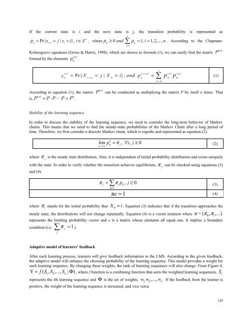
- Page 147 and 148: activities. Specifically, the histo
- Page 149 and 150: Huang, Y.-M., Huang, T.-C., Wang, K
- Page 151 and 152: • Could recommended learning sequ
- Page 153: Analysis of sequences prediction me
- Page 157 and 158: The figures 5a and 5b illustrate th
- Page 159 and 160: Learning sequence recommendation sy
- Page 161 and 162: In this study, forty subjects were
- Page 163 and 164: The potential for LSRS to promote l
- Page 165 and 166: They pointed out that LSRS helped t
- Page 167 and 168: Cover, T. M., & Thomas, J. A. (1991
- Page 169 and 170: Related Efforts An Internet forum i
- Page 171 and 172: with handheld devices and they were
- Page 173 and 174: agent would direct learners to a le
- Page 175 and 176: Mobile RSS Aggregator In order to s
- Page 177 and 178: learning, such as posting question
- Page 179 and 180: With novel technological support, m
- Page 181 and 182: Shen, L., Wang, M., & Shen, R. (200
- Page 183 and 184: as an ‘affective loop’, which r
- Page 185 and 186: Figure 2 is an example of two-dimen
- Page 187 and 188: preference was gathered through dat
- Page 189 and 190: compute the heart rate (HR) as a fu
- Page 191 and 192: sessions. Of all the 18 learning se
- Page 193 and 194: Burleson, W., Picard, R. W., Perlin
- Page 195 and 196: Wu, C.-C., & Lai, C.Y. (2009). Wire
- Page 197 and 198: The wireless handheld learning envi
- Page 199 and 200: the lengthiness of the scales, whic
- Page 201 and 202: Nursing dictionary We constructed a
- Page 203 and 204: them. The computers were networked
- Page 205 and 206:
“The major difference was that I
- Page 207 and 208:
questionnaire. We do not consider t
- Page 209 and 210:
Faruque, F., Hewlett, P. O., Wyatt,
- Page 211 and 212:
etween a user and the system. Addit
- Page 213 and 214:
Figure 2. A concept map representin
- Page 215 and 216:
C5.0 can help teachers to generate
- Page 217 and 218:
that a selected programming exercis
- Page 219 and 220:
differences between our system and
- Page 221 and 222:
1(students can complete without any
- Page 223 and 224:
The PADS sometimes assigned very di
- Page 225 and 226:
Corno, L. (2000). Looking at Homewo
- Page 227 and 228:
Hwang, W.-Y., Hsu, J.-L., Tretiakov
- Page 229 and 230:
listed these functions as allowing
- Page 231 and 232:
In the research presented in this a
- Page 233 and 234:
Research Tools Web-based learning e
- Page 235 and 236:
Table 1. Operational definitions of
- Page 237 and 238:
action, interaction, and outeractio
- Page 239 and 240:
for them was getting the answer as
- Page 241 and 242:
Table 6 shows the learners’ prefe
- Page 243 and 244:
Bell, P., & Winn, W. (2000). Distri
- Page 245 and 246:
Askar, P., & Altun, A. (2009). CogS
- Page 247 and 248:
elations, interactions and activiti
- Page 249 and 250:
Figure 3. A comparison of knowledge
- Page 251 and 252:
ontology will easily be extensible
- Page 253 and 254:
Figure 7. Visual Representation of
- Page 255 and 256:
Step 5: Use Boolean to combine the
- Page 257 and 258:
2) CogSkillNet provides classroom i
- Page 259 and 260:
Neo, M., & Neo, T.-K. (2009). Engag
- Page 261 and 262:
• Conversation and collaboration
- Page 263 and 264:
IMAGE 2 2. Problem identification I
- Page 265 and 266:
Methodology At the end of the proje
- Page 267 and 268:
presentation skills (m = 3.72), and
- Page 269 and 270:
6. Can’t be denying that, sometim
- Page 271 and 272:
Lambert, N. M., & McCombs, B. J. (1
- Page 273 and 274:
not detected in a previous study, t
- Page 275 and 276:
et al. (2001) studied the learning
- Page 277 and 278:
all the students. At the midpoint o
- Page 279 and 280:
The observed pairs were aware of be
- Page 281 and 282:
Table 2 shows the results from a mo
- Page 283 and 284:
Table 5: The distribution of time (
- Page 285 and 286:
As discussed in the section on prev
- Page 287 and 288:
McDowell, C., Werner, L., Bullock,
- Page 289 and 290:
Comprehension monitoring is the awa
- Page 291 and 292:
or roles in a context, such as “I
- Page 293 and 294:
Correlation coefficient was also co
- Page 295 and 296:
(a) Text 1 (b) Text 2 (c) Text 3 (d
- Page 297 and 298:
Table 3 shows that the average read
- Page 299 and 300:
Figure 10. Trace results of the les
- Page 301 and 302:
monitor their reading process and h
- Page 303 and 304:
Conn, S. R., Roberts, R. L., & Powe
- Page 305 and 306:
The technology-mediated groups, wit
- Page 307 and 308:
hybrid model of supervision was pos
- Page 309 and 310:
Our research indicates that the hyb
- Page 311 and 312:
Janoff, D. S., & Schoenholtz-Read,
- Page 313 and 314:
goal of using storyboards. But, thi
- Page 315 and 316:
In general, learning activities nee
- Page 317 and 318:
Furthermore, free subjects, such as
- Page 319 and 320:
Storyboarding Roots and related wor
- Page 321 and 322:
Referees, on the other hand, may wa
- Page 323 and 324:
Symbols Interpretation Defines a un
- Page 325 and 326:
Figure 4. Top-level storyboard for
- Page 327 and 328:
may take subjects such as practical
- Page 329 and 330:
network security information envir
- Page 331 and 332:
The concrete procedure and interact
- Page 333 and 334:
(e.g., for graduation) using such i
- Page 335 and 336:
Thus, academic education modeling b
- Page 337 and 338:
Feyer, T., Kao, O., Schewe, K.-D.,
- Page 339 and 340:
Richards, G. (2009). Book review: T
- Page 341 and 342:
expands the child’s proximal envi
- Page 343:
Chapter 6 exemplifies the activitie