Output frequency response function-based analysis for nonlinear ...

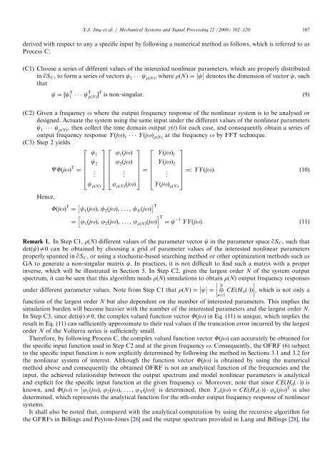
derived with respect to any a specific input by following a numerical method as follows, which is referred to as
Process C:
(C1) Choose a series of different values of the interested nonlinear parameters, which are properly distributed
in qSC, to form a series of vectors c1 that
crðNÞ, where rðNÞ ¼ c denotes the dimension of vector c, such
c ¼½c T
1 c T
rðNÞŠT is non singular: (9)
(C2) Given a frequency o where the output frequency response of the nonlinear system is to be analysed or
designed. Actuate the system using the same input under the different values of the nonlinear parameters
c1 crðNÞ, then collect the time domain output y(t) for each case, and consequently obtain a series of
output frequency response YðjoÞ1 YðjoÞrðNÞ at the frequency o by FFT technique.
(C3) Step 2 yields
CFðjoÞ T 2 3 2 3 2 3
c1 j1ðjoÞ YðjoÞ1 6 c
7 6
2 7 j
7 6
6 2ðjoÞ 7 YðjoÞ
7
6 2 7
6 7 6 7 6 7
¼ 6 . 7 6
6
4 . 7 . 7 ¼ 6
6
5 4 . 7 . 7 ¼: YYðjoÞ. (10)
6
5 4 . 7
5
crðNÞ jrðNÞðjoÞ YðjoÞrðNÞ Hence,
ARTICLE IN PRESS
X.J. Jing et al. / Mechanical Systems and Signal Processing 22 (2008) 102–120 107
FðjoÞ T ¼ f1ðjoÞ; f2ðjoÞ; ...; fNðjoÞ T
h iT ¼ j1ðjoÞ; j2ðjoÞ; ...; jrðNÞðjoÞ ¼ c 1 YYðjoÞ. ð11Þ
Remark 1. In Step C1, r(N) different values of the parameter vector c in the parameter space qSC, such that
detðcÞa0 can be obtained by choosing a grid of parameter values of the interested nonlinear parameters
properly spanned in qSC, or using a stochastic-based searching method or other optimization methods such as
GA to generate a non-singular matrix c. In practices, it is not difficult to find such a matrix with a proper
inverse, which will be illustrated in Section 5. In Step C2, given the largest order N of the system output
spectrum, it can be seen that this algorithm needs r(N) simulations to obtain r(N) output frequency responses
under different parameter values. Note from Step C1 that rðNÞ ¼ c ¼ CEðHnð ÞÞ , which is not only a
n¼1
function of the largest order N but also dependent on the number of interested parameters. This implies the
simulation burden will become heavier with the number of the interested parameters and the largest order N.
In Step C3, since detðcÞa0, the complex valued function vector F(jo) in Eq. (11) is unique, which implies the
result in Eq. (11) can sufficiently approximate to their real values if the truncation error incurred by the largest
order N of the Volterra series is sufficiently small.
Therefore, by following Process C, the complex valued function vector F(jo) can accurately be obtained for
the specific input function used in Step C2 and at the given frequency o. Consequently, the OFRF (6) subject
to the specific input function is now explicitly determined by following the method in Sections 3.1 and 3.2 for
the nonlinear system of interest. Although the function vector F(jo) is obtained by using the numerical
method above and consequently the obtained OFRF is not an analytical function of the frequencies and the
input, the achieved relationship between the output spectrum and model nonlinear parameters is analytical
and explicit for the specific input function at the given frequency o. Moreover, note that since CE(Hn( )) is
known, and FðjoÞ ¼ j1ðjoÞ; j2ðjoÞ; ...; jNðjoÞ is determined, then Y nðjoÞ ¼CEðHnð ÞÞ jnðjoÞ T is also
determined, which represents the analytical function for the nth-order output frequency response of nonlinear
systems.
It shall also be noted that, compared with the analytical computation by using the recursive algorithm for
the GFRFs in Billings and Peyton-Jones [26] and the output spectrum provided in Lang and Billings [28], the
N