JavaPsi - Simulating and Visualizing Quantum Mechanics (english)

3 SOLVING SCHRÖDINGER’S EQUATION 6
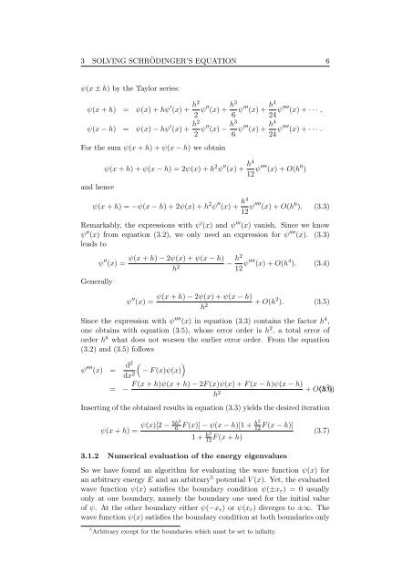
ψ(x ± h) by the Taylor series:
ψ(x + h) = ψ(x) + hψ ′ (x) + h2
2 ψ′′ (x) + h3
6 ψ′′′ (x) + h4
24 ψ′′′′ (x) + · · · ,
ψ(x − h) = ψ(x) − hψ ′ (x) + h2
2 ψ′′ (x) − h3
6 ψ′′′ (x) + h4
24 ψ′′′′ (x) + · · · .
For the sum ψ(x + h) + ψ(x − h) we obtain
and hence
ψ(x + h) + ψ(x − h) = 2ψ(x) + h 2 ψ ′′ (x) + h4
12 ψ′′′′ (x) + O(h 6 )
ψ(x + h) = −ψ(x − h) + 2ψ(x) + h 2 ψ ′′ (x) + h4
12 ψ′′′′ (x) + O(h 6 ). (3.3)
Remarkably, the expressions with ψ ′ (x) and ψ ′′′ (x) vanish. Since we know
ψ ′′ (x) from equation (3.2), we only need an expression for ψ ′′′′ (x). (3.3)
leads to
ψ ′′ (x) =
Generally
ψ(x + h) − 2ψ(x) + ψ(x − h)
h 2
ψ ′′ (x) =
− h2
12 ψ′′′′ (x) + O(h 4 ). (3.4)
ψ(x + h) − 2ψ(x) + ψ(x − h)
h 2 + O(h 2 ). (3.5)
Since the expression with ψ ′′′′ (x) in equation (3.3) contains the factor h 4 ,
one obtains with equation (3.5), whose error order is h 2 , a total error of
order h 6 what does not worsen the earlier error order. From the equation
(3.2) and (3.5) follows
ψ ′′′′ (x) = d2
dx2
− F (x)ψ(x)
F (x + h)ψ(x + h) − 2F (x)ψ(x) + F (x − h)ψ(x − h)
= −
h2 + O(h 2 (3.6) ).
Inserting of the obtained results in equation (3.3) yields the desired iteration
ψ(x + h) =
ψ(x)[2 − 5h2
6
h2
F (x)] − ψ(x − h)[1 + 12 F (x − h)]
1 + h2
12 F (x + h)
3.1.2 Numerical evaluation of the energy eigenvalues
(3.7)
So we have found an algorithm for evaluating the wave function ψ(x) for
an arbitrary energy E and an arbitrary 5 potential V (x). Yet, the evaluated
wave function ψ(x) satisfies the boundary condition ψ(±xr) = 0 usually
only at one boundary, namely the boundary one used for the initial value
of ψ. At the other boundary either ψ(−xr) or ψ(xr) diverges to ±∞. The
wave function ψ(x) satisfies the boundary condition at both boundaries only
5 Arbitrary except for the boundaries which must be set to infinity.