Chapter 4 Vortex detection - Computer Graphics and Visualization

Chapter 2. Geometry extraction techniques
in a grid cell. The intersection curve of these stream surfaces is a streamline segment,
which is approximated by determining the entry and exit points of the streamline segment
in the cell, and connecting these points. A stream line is constructed by tracking
from a starting point through the cells. This technique is very different from the time
stepping integration techniques described in Section 3.1, and has the advantage of conforming
with the physical law of mass conservation.
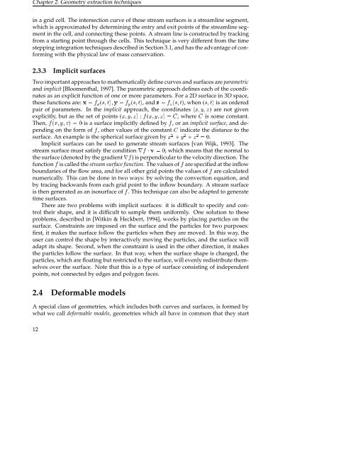
2.3.3 Implicit surfaces
Two important approaches to mathematically define curves and surfaces are parametric
and implicit [Bloomenthal, 1997]. The parametric approach defines each of the coordinates
as an explicit function of one or more parameters. For a 2D surface in 3D space,
these functions are: Ü Ü × Ø Ý Ý × Ø , and Þ Þ × Ø , when × Ø is an ordered
pair of parameters. In the implicit approach, the coordinates Ü Ý Þ are not given
explicitly, but as the set of points Ü Ý Þ Ü Ý Þ , where is some constant.
Then, Ü Ý Þ is a surface implicitly defined by , oranimplicit surface, and depending
on the form of , other values of the constant indicate the distance to the
surface. An example is the spherical surface given by Ü Ý Þ .
Implicit surfaces can be used to generate stream surfaces [van Wijk, 1993]. The
stream surface must satisfy the condition Ö ¡ Ú , which means that the normal to
the surface (denoted by the gradient Ö) is perpendicular to the velocity direction. The
function is called the stream surface function. The values of are specified at the inflow
boundaries of the flow area, and for all other grid points the values of are calculated
numerically. This can be done in two ways: by solving the convection equation, and
by tracing backwards from each grid point to the inflow boundary. A stream surface
is then generated as an isosurface of . This technique can also be adapted to generate
time surfaces.
There are two problems with implicit surfaces: it is difficult to specify and control
their shape, and it is difficult to sample them uniformly. One solution to these
problems, described in [Witkin & Heckbert, 1994], works by placing particles on the
surface. Constraints are imposed on the surface and the particles for two purposes:
first, it makes the surface follow the particles when they are moved. In this way, the
user can control the shape by interactively moving the particles, and the surface will
adapt its shape. Second, when the constraint is used in the other direction, it makes
the particles follow the surface. In that way, when the surface shape is changed, the
particles, which are floating but restricted to the surface, will evenly redistribute themselves
over the surface. Note that this is a type of surface consisting of independent
points, not connected by edges and polygon faces.
2.4 Deformable models
A special class of geometries, which includes both curves and surfaces, is formed by
what we call deformable models, geometries which all have in common that they start
12