HEAT TRANSFER AND SOLIDIFICATION MODEL OF ...

Metallurgical and Materials Transactions B, Vol. 34B, No. 5, Oct., 2003, pp. 685-705.
HEAT TRANSFER AND SOLIDIFICATION MODEL
OF CONTINUOUS SLAB CASTING: CON1D
Ya Meng and Brian G. Thomas
University of Illinois at Urbana-Champaign,
Department of Mechanical and Industrial Engineering,
1206 West Green Street,
Urbana, IL USA 61801
Ph: 217-333-6919; Fax: 217-244-6534; Email: bgthomas@uiuc.edu
ABSTRACT
A simple, but comprehensive model of heat transfer and solidification of the continuous
casting of steel slabs is described, including phenomena in the mold and spray regions. The
model includes a 1-D transient finite-difference calculation of heat conduction within the
solidifying steel shell coupled with 2-D steady-state heat conduction within the mold wall. The
model features a detailed treatment of the interfacial gap between the shell and mold, including
mass and momentum balances on the solid and liquid interfacial slag layers, and the effect of
oscillation marks. The model predicts shell thickness, temperature distributions in the mold
and shell, thickness of the re-solidified and liquid powder layers, heat flux profiles down the
wide and narrow faces, mold water temperature rise, ideal taper of the mold walls, and other
related phenomena. The important effect of non-uniform distribution of superheat is incorporated
using the results from previous 3-D turbulent fluid flow calculations within the liquid pool. The
FORTRAN program, CON1D, has a user-friendly interface and executes in less than a minute on
a personal computer. Calibration of the model with several different experimental measurements
on operating slab casters is presented along with several example applications. In particular,
the model demonstrates that the increase in heat flux throughout the mold at higher casting
speeds is caused by two combined effects: thinner interfacial gap near the top of the mold, and

thinner shell towards the bottom. This modeling tool can be applied to a wide range of
practical problems in continuous casters.
I. INTRODUCTION
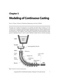
Heat transfer in the continuous slab casting mold is governed by many complex phenomena.
Figure 1 shows a schematic of some of these. Liquid metal flows into the mold cavity through a
submerged entry nozzle, and is directed by the angle and geometry of the nozzle ports [1] . The
direction of the steel jet controls turbulent fluid flow in liquid cavity, which affects delivery of
superheat to solid/liquid interface of the growing shell. The liquid steel solidifies against the four
walls of the water-cooled copper mold, while it is continuously withdrawn downward at the
casting speed.
Mold powder added to the free surface of the liquid steel melts and flows between the steel
shell and the mold wall to act as a lubricant [2] , so long as it remains liquid. The resolidified mold
powder, or “slag”, adjacent to the mold wall cools and greatly increases in viscosity, thus acting
like a solid. It is thicker near and just above the meniscus, where it is called the “slag rim”. The
slag cools rapidly against the mold wall forming a thin solid glassy layer, which can devitrify to
form a crystalline layer if its residence time in the mold is very long [3] . This relatively solid slag
layer often remains stuck to the mold wall, although it is sometimes dragged intermittently
downward at an average speed less than the casting speed [4] . Depending on its cooling rate, this
slag layer may have a structure that is glassy, crystalline or a combination of both [5] . So long as
the steel shell remains above its crystallization temperature, a liquid slag layer will move
downward, causing slag to be consumed at a rate balanced by the replenishment of bags of solid
powder to the top surface. Still more slag is captured by the oscillation marks and other
imperfections of the shell surface and carried downward at the casting speed.
2

These layers of mold slag comprise a large resistance to heat removal, although they provide
uniformity relative to the alternative of an intermittent vapor gap found with oil casting of billets.
Heat conduction across the slag depends on the thickness and conductivity of its layers, which in
turn depends on their velocity profile, crystallization temperature [6] , viscosity, and state (glassy,
crystalline or liquid). The latter can be determined by the Time-Temperature-Transformation
(TTT) diagram measured for the slag, knowing the local cooling rate [7-9] . Slag conductivity
depends mainly on the crystallinity of the slag layer and on the internal evolution of its dissolved
gas to form bubbles.
Shrinkage of the steel shell away from the mold walls may generate contact resistances or air
gaps, which act as a further resistance to heat flow, especially after the slag is completely solid
and unable to flow into the gaps. The surface roughness depends on the tendency of the steel
shell to “ripple” during solidification at the meniscus to form an uneven surface with deep
oscillation marks. This depends on the oscillation practice, the slag rim shape and properties, and
the strength of the steel grade relative to ferrostatic pressure, mold taper, and mold distortion.
These interfacial resistances predominantly control the rate of heat flow in the process.
Finally, the flow of cooling water through vertical slots in the copper mold withdraws the
heat and controls the temperature of the copper mold walls. If the “cold face” of the mold walls
becomes too hot, boiling may occur, which causes variability in heat extraction and
accompanying defects. Impurities in the water sometimes form scale deposits on the mold cold
face, which can significantly increase mold temperature, especially near the meniscus where the
mold is already hot. After exiting the mold, the steel shell moves between successive sets of
alternating support rolls and spray nozzles in the spray zones. The accompanying heat
extraction causes surface temperature variations while the shell continues to solidify.
3

It is clear that many diverse phenomena simultaneously control the complex sequence of
events which govern heat transfer in the continuous casting process. The present work was
undertaken to develop a fast, simple, and flexible model to investigate these heat transfer
phenomena. In particular, the model features a detailed treatment of the interfacial gap in the
mold, which is the most important thermal resistance. The model includes heat, mass,
momentum and force balances on the slag layers in the interfacial gap.
This model is part of a larger comprehensive system of models of fluid flow, heat transfer,
and mechanical behavior, which is being developed and applied to study the formation of defects
in the continuous casting process. These other models are used to incorporate the effects of mold
distortion [10] , the influence of fluid flow in the liquid pool on solidification of the shell [11] , and
coupled thermal stress analysis of the shell to find the reduction of heat transfer across the
interface due to air gap formation [12] .
This paper first describes the formulation of this model, which has been implemented into a
user-friendly FORTRAN program, CON1D, on personal computers and UNIX workstations.
Then, validation of the model with analytical solutions and calibration with example plant
measurements are presented. Finally the effect of casting speed on mold heat transfer is
investigated as one example of the many applications of this useful modeling tool.
II. PREVIOUS WORK
Many mathematical models have been developed of the continuous casting process, which
are partly summarized in previous literature reviews [13-15] . Many continuous casting models are
very sophisticated (even requiring supercomputers to run) so are infeasible for use in an
operating environment. The earliest solidification models used 1-D finite difference methods to
calculate the temperature field and growth profile of the continuous cast steel shell [16, 17] . Many
industrial models followed [18, 19] . These models first found application in the successful prediction
4

of metallurgical length, which is also easily done by solving the following simple empirical
relationship for distance, z, with the shell thickness, S, set to half the section thickness.
S = K z Vc
[1]
where K is found from evaluation of breakout shells and computations. Such models found
further application in trouble shooting the location down the caster of hot tear cracks initiating
near the solidification front [20] , and in the optimization of cooling practice below the mold to
avoid subsurface longitudinal cracks due to surface reheating [21] .
Since then, many advanced models have been developed to simulate further phenomena such
as thermal stress and crack related defects [12, 22, 23] or turbulent fluid flow [24-28] coupled together
with solidification. For example, a 2-D transient stepwise coupled elasto-viscoplastic finite-
element model tracks the behavior of a transverse slice through a continuously cast rectangular
strand as it moves down through the mold at casting speed [12] . This model is suited for simulating
longitudinal phenomena such as taper design [29] , longitudinal cracks [30] and surface depressions [31] .
Other casters have been modeled using 3-D coupled fluid flow – solidification models [27] based
on control-volume or finite difference approaches at the expense of greater computation time and
memory.
To study temperature distribution and/or distortion of the mold, 3-D finite-element thermal-
stress models have been applied [10, 32] . These models have been crucial in determining the axial
heat flux profile based on measured temperatures in the mold walls [20, 32, 33] . This procedure is
sometimes automated with inverse heat conduction models [20] .
One of the greatest resistances to heat transfer from the liquid steel to the mold cooling water
is the interface between the mold and shell. Heat transfer across this interface is controlled by the
thickness and thermal properties of the materials that fill the gap. Despite its known importance,
most previous mathematical models characterize the interface as a boundary condition for a
5

model of either the shell or the mold alone. Even models of both usually use a simplified
treatment of the gap [34-36] .
A few models have considered more detailed treatment of the resolidified powder layers in
the gap, and calculate slag layer thicknesses [37, 38] , slag velocity profile along the film thickness [38,
39] and interface friction [37-39] . Common oversimplifications include neglecting the solid slag
layer [40] , assuming constant slag layer thickness [39] , or assuming constant slag viscosity [41, 42] . The
highly temperature-dependent slag viscosity has been modeled with a simple inverse function of
temperature [38] or with an Arrhenius equation [37, 39, 43] , by fitting the low viscosities (usually less
than 10Pa⋅s) measured at high temperature and then extrapolating to lower temperatures. Even
the best interface models generally oversimplify the shell and/or the mold. Thus, there is a
need for a comprehensive model of the shell, mold, and gap, which is fast and easy to run, for
use in both research and steel plant environments.
III. MODEL FORMULATION
The model in this work computes 1-D transient heat flow through the solidifying steel shell,
coupled with 2-D steady-state heat conduction within the mold wall. Superheat from the liquid
steel was incorporated as a heat source at the steel solid/liquid interface. The model features a
detailed treatment of the interfacial gap, including mass and momentum balances on the liquid
and solid slag layers, friction between the slag and mold, and slag layer fracture. The model
simulates axial (z) behavior down a chosen position on the mold perimeter. Wide-face, narrow-
face and even corner simulations can thus be conducted separately.
A Superheat Delivery
Before it can solidify, the steel must first cool from its initial pour temperature to the liquidus
temperature. Due to turbulent convection in the liquid pool, this “superheat” contained in the
6

liquid is not distributed uniformly. A small database of results from a 3-D fluid flow model [11] is
used to determine the heat flux, qsh, delivered to the solid/liquid interface due to the superheat
dissipation, as a function of distance below the meniscus. The initial condition of the liquid
steel at the meniscus is then simply the liquidus temperature.
Previous work [11] found that this “superheat flux” varies linearly with superheat temperature
difference and also is almost directly proportional to casting speed. The superheat flux function
in the closest database case is adjusted to correspond with the current superheat temperature
difference, ∆Tsup, and casting speed, Vc, as follows:
where
∆T
V
o sup c
sh = sh o o
∆Tsup
Vc
q q
o
qsh is the superheat flux profile from the database case with conditions of superheat
o
temperature difference ∆Tsup and casting speed
[2]
o
V c . Further adjustments are made to translate
the heat flux peak to account for differences in nozzle configuration between the current
conditions and the database. Examples of the superheat flux function are included in Fig.2,
which represents results for a typical bifurcated, downward-directed nozzle. The influence of this
function is insignificant to shell growth over most of the wide face, where the superheat flux is
small and contact with the mold is good.
B Heat Conduction in the Solidifying Steel Shell
Temperature in the thin solidifying steel shell is governed by the 1-D transient heat
conduction equation, which becomes the following on applying the chain rule to the
temperature-dependent conductivity:
ρ
2
* ∂T T steel ∂T
steelCpsteel ksteel
2
2
∂ ∂ k ⎛ ⎞
= + ⎜ ⎟
∂t ∂x ∂T ⎝∂x ⎠ [3]
7

Temperature dependent properties are given in Appendix D [44, 45] . Both sensible and latent heat
of steel are included in the effective specific heat, Cp , explained in Section IV-C.
This equation assumes that axial (z) heat conduction is negligible in the steel, which is
reasonable past the top 10mm, due to the large advection component as indicated by the large
Péclet number:
*
steel
VZ c mold ρ steelCpsteel 0.0167× 0.81× 7400× 670
Pe = = = 2236. The simulation
k
30
steel
domain for this portion of the model is a slice through the liquid steel and solid shell, which
moves downward at the casting speed, as pictured in Figs. 2 and A-1 together with typical
interface conditions. At the internal solid/liquid steel interface, the “superheat flux”, qsh,
delivered from the turbulent liquid pool, (Section III A), is imposed as a source term. From the
external surface of the shell, interfacial heat flux, qint, is lost to the gap, which depends on the
mold and slag layer computations, described in the following two sections. Appendix A provides
the explicit finite-difference solution of Eq.3, including both of these boundary conditions.
C Heat transfer Across the Interfacial Gap
Heat transfer across the interfacial gap governs the heat flux leaving the steel, qint, to enter
the mold. To calculate this at every position down the mold, the model evaluates an effective
heat transfer coefficient, hgap, between the surface temperature of the steel shell, Ts, and the hot
face of the mold wall, Tmold:
( )
q = h T − T
[4]
int gap s mold
⎛⎛ dair d ⎞ ⎛ ⎛d solid
liquid d ⎞ ⎞⎞
eff
hgap = 1 ⎜ rcontact + + + 1 ⎜1 ⎜ + ⎟+
h ⎟ rad ⎟
⎜
⎜ ⎟
kair k ⎜ ⎜
solid kliquid k ⎟
⎝ ⎠
⎟
⎝
⎟
eff
⎝ ⎝ ⎠ ⎠⎠
Heat conduction depends on the thermal resistances of four different layers of materials
contained in the gap: oscillation marks, liquid slag, solid slag and a possible air gap. These
[5]
8

depend on the time-averaged thickness profiles down the mold of the different layers and their
corresponding thermal conductivities. The model for gap heat conduction is illustrated in Figs.3
and 6. The most important resistances are usually the slag layers, whose thicknesses are
calculated as described in the next section. The latent heat evolved by liquid slag solidification is
less than 3% of the heat transferred across the gap, so it is neglected in this model.
The equivalent air gap, dair, is specified as input data and includes contact resistances [46] at the
slag/shell and slag/mold interfaces. It may also include a gap due to shrinkage of the steel shell,
which can be calculated using a separate thermal-stress model [12] . The shrinkage gap is affected
by the mold taper and also by mold distortion, which can be calculated by another model [10] . This
gap is important when simulating down positions near the corner.
All non-uniformities in the flatness of the shell surface are incorporated into the model
through the prescribed oscillation mark depth, dmark, and width, Lmark, as pictured in Fig.4.
Assuming shallow triangle-shaped marks or depressions, dosc is the volume-averaged oscillation
mark depth:
d
osc
0.5Lmarkdmark = [6]
L
pitch
where Lpitch is the ratio of the casting speed Vc to the oscillation frequency, freq.
The oscillation marks affect heat transfer in two different ways. Firstly, the oscillation marks
consume mold slag, so affect the slag layer thicknesses, as described in section F. Secondly, they
reduce heat conduction by effectively providing an extra gap. This extra gap is represented by
deff, calculated based on a heat balance [47] which produces the same total heat flux as found by
combining the heat fluxes across the two parallel conduction paths (at or adjacent to the
oscillation mark), averaged spatially (z-direction) using an appropriate weighted average.
9

d
eff
=
L − L
0.5 Lmarkdmark ⎛ dmark
⎜1+ 0.5
⎜
⎝ dliquid + dsolid k ⎞ gap
⎟+
L
k ⎟
mark ⎠
( )
pitch mark mark
⎛d⎛ k
⎞⎞
solid
liquid
kgap= ( dliquid + dsolid ) ⎜ + 1 ⎜ + hrad
_ liquid ⎟⎟
⎜ k ⎜
solid d
⎟⎟
⎝ ⎝ liquid ⎠⎠
The oscillation marks are assumed to be filled with either slag, air, or a mixture, depending on
the local shell surface temperature. This governs the value of kmark.
Except for perhaps a microscopically thin glassy surface layer, experience has shown that the
cold slag layer adjacent to the mold wall is usually crystalline [48, 49] , and thus opaque. Thus,
radiation occurs only across the semi-transparent hot glassy or liquid layer above Tfsol [50, 51] ,
according to Eq.9, as shown in Fig.3:
( sK +
2
fsolK )( sK + fsolK)
( liquid eff )
1 1
2 2
m σ T T T T
rad = mold < fsol
( )
h T T
0.75a d + d +
ε
+
ε
−1
slag steel
where m is slag refractive index; TsK and Tfsol K are Ts and Tfsol expressed in Kelvin, a is average
absorption coefficient of the slag, assuming graybody radiation (εslag =0.9). If the liquid slag runs
out, so that Ts< T , then hrad=0. In the unlikely event that fsol
Tmold ≥ Tfsol
[7]
[8]
[9]
10
, εslag would be replaced
by εmold, and Tfsol by Tmold in Eq.9. Jenkins showed that this simple equation to characterize
radiation with absorption across a gap, Eq.9, is accurate to within 10% relative to a full multi-
view factor analysis including radiation-conduction [52] . This is sufficiently accurate because the
radiation component itself usually contributes only on the order of 10% of the gap heat transfer.

D Mass and Momentum Balance on Powder Slag Layers
Slag is assumed to flow down the gap as two distinct layers: solid and liquid. The solid layer
is assumed to move at a time-average velocity, Vsolid, which is always between zero and the
casting speed, Vc, according to the input solid slag speed ratio, fv.
Vsolid = fv⋅ Vc
[10]
The downward velocity profile across the liquid slag layer is governed by the simplified
Navier-Stokes equation, assuming laminar Couette flow:
∂ ⎛ ∂Vz
⎞
⎜µ ⎟=
ρ −ρ
∂x⎝ ∂x
⎠
( steel slag )
g
A small body force opposing flow down the wide face gap is created by the difference
between the ferrostatic pressure from the liquid steel, ρ steel g, transmitted through the solid steel
shell, and the average weight of the slag, ρ slag g. The time-average velocity of the liquid slag
described by Eq.11, Vz, is subjected to boundary conditions constraining it to the casting speed,
Vc on its hot side and to the solid slag velocity, Vsolid on its cold side.
The viscosity of the molten slag, µ(T), is assumed to vary exponentially with temperature:
n
⎛To T ⎞ fsol
o
T Tfsol
−
⎜ − ⎟
⎝ ⎠
µ = µ ⎜ ⎟
where the parameters Tfsol and n are chosen empirically to fit measured data and µo is the
viscosity measured at the reference temperature, To, usually chosen to be 1300 o C. A typical
curve obtained with this function is shown in Fig.5 together with the measured viscosities by
Lanyi that it was fit to match [53] . Mold slag in service absorb some Al2O3 from the steel, which
changes their properties, including decreasing the solidification temperature [53, 54] . The second
curve in Fig.5 was constructed for a reported solidification temperature Tfsol of 1045 o C and
viscosity at 1300 o C of 1.1Poise, and was used later in model calibration.
[11]
[12]
11

By approximating temperature across the gap to vary linearly, Eqs.10-12 can be solved for
the time-averaged velocity distribution across the slag layers, which is illustrated in Fig.6.
Integrating across the liquid region yields an average velocity for the liquid layer, V liquid :
V
liquid
( ρ ρ )
s
2
( n+ 2) ( n+
3)
( 1)
( n + 2)
2
slag − steel gd V liquid c + Vsolid n+
= +
µ
where µs is the slag viscosity at liquid layer/steel shell interface. A mass balance was imposed to
match the measured (known) powder consumption, Qslag(kg/m 2 ), with the total molten slag flow
rate past every location down the interfacial gap, neglecting the carbon content component,
which burns off. This consumption rate is expressed as mass of slag per unit area of the strand
surface, which can be found from the consumption per mass of product, Mslag(kg/ton) :
2
W× N
Qslag ( kg/ m ) = Mslag ( kg/ ton)
× ρsteel
×
2
( W + N)
where W is slab width and N is slab thickness. Slag can be carried downward by the solid layer,
the liquid layer, and in the oscillations marks:
Q × V
slag c
ρ
slag
solid solid liquid liquid c osc
[13]
[14]
= V d + V d + V d
[15]
The liquid and solid layer thicknesses are obtained by solving a fourth order polynomial equation
found by combining Eqs.5 and 15. The transport of slag by the oscillation marks depends on
the lubrication state, discussed next.
Three different regions are distinguished down the mold, according to the lubrication
condition. Close to the meniscus, a solid slag rim exists against the mold wall. Its thickness
profile must be specified, as it depends on transient phenomena not yet in the model.
The second region, shown in Fig.6, allows the solid slag layer to move at the slow time
averaged velocity Vsolid. It always also includes oscillation marks filled with molten slag and a
12

continuous liquid slag layer, which remains present so long as the outer surface temperature of
the steel Ts’ exceeds the slag solidification temperature, Tfsol:
T T q
d
'
eff
s = s − int ⋅ [16]
kmark
Slag in the oscillation marks remains liquid longer, due to the higher local shell temperature
at their roots, Ts. Once the oscillation mark roots cool below the slag solidification temperature,
however, the slag entrapped in them solidifies. This defines the third region, which consists of
totally solid slag, moving downward at the uniform speed, Vsolid. The oscillation marks no longer
transport slag, so become filled with air. The transition between the second and third regions is
gradual.
It is important to emphasize that this model represents steady, time-averaged behavior only.
To investigate transient phenomena, a transient version of this model is being developed to
calculate stress inside the slag layer based on force balance with friction, which is described
elsewhere [55] .
E Heat Conduction in the Mold
Two dimensional, steady state temperature within a rectangular vertical section through the
upper portion of the mold is calculated assuming constant conductivity:
2 2
∂ T ∂ T
+ = 0
2 2
∂x ∂z
This equation is solved using a standard Fourier series product solution [56] applying fixed heat
flux, int mold T
q =−k
∂
∂ x
, and convection, hwater and Twater as boundary conditions, as shown in
Fig.7a. This copper domain is generally chosen to extend from the top of the mold to 100mm
below the meniscus. Below this meniscus region, heat flow is one-dimensional through the
thickness. Temperature at the copper hot face, Thotc, is then:
[17]
13

T T q
⎛ 1 d ⎞ mold +
hotc = water + int ⎜ ⎟
hwater kmold
⎝ ⎠
where dmold is the copper mold thickness calculated in Appendix B. Coating layers are
incorporated as needed to find the mold hot face temperature, Tmold, by adding extra dcoat/kcoat
resistances to Eq.18 as needed. In addition to the heat flux across the interface, qint, this
calculation requires the initial cooling water temperature, Twater, input as a boundary condition,
and the effective water heat transfer coefficient, hwater, discussed next.
F Convection to the Cooling Water
The effective heat transfer coefficient between the cooling water and the cold face (“water-
side”) of the mold, hwater, is calculated including a possible resistance due to scale deposits on the
surface of the cooling water channels:
h
water
⎛dscale 1 ⎞
= 1 ⎜ +
⎜
⎟
kscale h ⎟
⎝ fin ⎠
To account for the complex nature of heat flow in the undiscretized width direction of the
mold, the heat transfer coefficient between the mold cold face and the cooling water, hfin,
incorporates heat flow to both the root and sides of the water channels, the latter treated as heat-
transfer fins.
h
fin
( − )
2
hw 2hk w mold Lch wch 2hd
w ch
w ch
= +
tanh
L L k L w
( − )
ch ch mold ch ch
where the mold geometry parameters, Lch, wch, and dch are shown in Fig.7b. The heat transfer
coefficient between the water and the sides of the water channel, hw, is calculated assuming
turbulent flow through an equivalent-diameter pipe using the empirical correlation of Sleicher
and Reusse [57] , which is reported [58] to be more accurate than other relations such as Dittus and
Boelter [59] :
[18]
[19]
[20]
14

where
h
k
c1 c2
= ( 5 + 0.015Re Pr )
[21]
D
water
w waterf waterw
2wchdch D =
w + d
ch ch
c 1 = 0.88 − 0.24 ( 4 + Prwaterw ) ,
is the equivalent diameter of the water channel,
c e −
= + are empirical constants.
0.6Prwaterw
2 0.333 0.5
The presence of the water slots can either enhance or diminish the heat transfer, relative to a
tube mold with uniform thickness, dmold, such as used in billet casting. Deep, closely spaced slots
augment the heat transfer coefficient, (hfin larger than hw) while shallow, widely spaced slots
inhibit heat transfer. In most molds, hfin and hw are very close.
Although it slightly underpredicts mold temperature, Eq.20 was shown, through comparison
with many 3-D computations for a variety of typical slab casting mold geometries and
conditions, to match the temperature within 1% at the water slot root and from 0.1% to 6% at the
hot face [47, 60] . For a typical hot face temperature of 190 o C and water temperature of 30 o C, it gives
maximum errors of 2 o C and 10 o C. It is most accurate for molds with either deep, closely-spaced
slots [47] or very wide slots [60] , where cold face temperature is most nearly constant as assumed in
Eq.20.
G Spray zones below the mold
Below the mold, heat flux from the strand surface varies greatly between each pair of support
rolls according to spray nozzle cooling (based on water flux), hspray; radiation, hrad_spray; natural
convection, hconv; and heat conduction to the rolls, hroll, as shown in Fig.8. Incorporating these
phenomena enables the model to simulate heat transfer during the entire continuous casting
process. The heat extraction due to water sprays is a function of water flow [61] , of the following
form:
( 1 )
h = A⋅Q ⋅ −b⋅ T
[22]
spray
c
water spray
15

where Qwater (l/m 2 s) is water flux in spray zones, Tspray is the temperature of the spray cooling
water. In Nozaki’s empirical correlation [62] , A=0.3925, c=0.55, b=0.0075, which has been used
successfully by other modelers [61, 63] .
Radiation is calculated by:
2 2
( )( )
h = σ ⋅ ε T + T T + T
[23]
rad _ spray steel s K amb K s K spray K
where TsK and TsprayK are Ts and Tspray expressed in Kelvin. Natural convection is treated as a
constant input for every spray zone. For water-cooling only, it is not very important, so was
simplified to 8.7W/m 2 K everywhere. Larger values can be input for hconv to reflect the stronger
convection when there is air mist in the cooling zone. Heat extraction into the rolls is calculated
based on the fraction of heat extraction to the rolls, froll, which is calibrated for each spray zone:
( hrad _spray + hconv + hspray ) ⋅ Lspray + ( hrad _spray
+ hconv ) ⋅( Lspray pitch −Lspray −Lroll
contact )
h = ⋅ f
( 1 )
roll roll
Lrollcontact ⋅ − froll
A typical froll value of 0.05 produces local temperature drops beneath the rolls of about 100 o C.
Beyond the spray zones, heat transfer simplifies to radiation and natural convection.
H Solution Methodology
The model requires simultaneous solution of three different systems of equations: 1-D
transient heat conduction and solidification of the steel shell, 2-D steady state heat conduction in
the mold, and the equations balancing heat, mass and momentum in the gap. The simulation
starts by setting the initial steel and mold temperatures to the pouring temperature and inlet
cooling water temperature respectively. Phase transformation temperatures and phase fraction
temperature curves are then calculated, using one of the methods described in the next section.
Then, each time step begins by rearranging and solving Eqs.5 and 15 simultaneously for dliquid
and dsolid, based on heat and mass balance at the previous time step. The heat flux qint is then
[24]
16

calculated according to Eqs.4 and 5, which is the boundary condition for both steel and mold
domains. The heat transfer coefficient, hwater is calculated according to cooling channel
conditions with Eqs.19 to 21, and used to obtain mold temperatures. Applying the superheat flux
boundary condition, Eq.2, as an internal heat source at the steel solid/liquid interface, the model
uses an explicit, central-finite difference algorithm originally developed by Pehlke [64] to solve
Eq.3 for the shell temperature at each time step (Appendix A). This limits the maximum time
step size, ∆t. When a node temperature drops below the liquidus temperature, its solid fraction is
calculated from the latent heat evolved, and then the node temperature is adjusted [65] (Eq.A6)
according to the phase fraction-temperature curves, described in section IV-A. The results are
used as initial conditions for the 2-D mold calculation, which solves Eq.17 analytically, relating
distance down the mold, z, to time in the shell through the casting speed. Subsequently, the
entire 1-D shell solidification model in the 2-D mold region is recomputed using the new 2-D
mold temperatures as its boundary condition. This stepwise coupling procedure alternates
between models until the 1-D mold temperatures converge to match the 2-D results within 3 o C.
This produces a self-consistent prediction, which is stable for all coupled simulations
investigated and usually converges in 3-4 iterations. Figure 9 gives a flow chart of the whole
procedure.
The model has been incorporated into a user-friendly FORTRAN program, CON1D [66] . A
100-second long simulation with 0.004sec time step and 100-node mesh runs on a Pentium III
personal computer (using 3.1Mbytes of memory) in about 30 seconds.
IV. STEEL PROPERTIES
The program includes several different choices for steel properties, including simple
constants input by the user. By default, the liquidus temperature, solidus temperature, phase
fraction curve, thermal conductivity, specific heat and thermal linear expansion are all calculated
17

as functions of composition and temperature. Steel density, ρsteel, latent heat, Lf, and steel surface
emissivity, εsteel, are constants. For carbon steel: ρsteel =7400kg/m 3 , Lf =271kJ/kg, εsteel =0.8
A Phase Fraction
By default, equilibrium lever-rule calculations are performed on an Fe-C phase diagram,
whose phase field lines are specified as simple linear functions of alloy content (including the
influences of Si, Cr, Mn, Ni, Mo, Cu, Ti, P, S, Al, V, N, Nb and W) reported by Kagawa and
Okamoto [67] in order to calculate steel liquidus, solidus, peritectic temperature and phase
fractions. Alternatively, the user can choose a non-equilibrium micro-segregation model to find
these values, based on an analytical Clyne-Kurz style equation developed by Won and
Thomas [68] , which was extended in this work to include the effects of 14 elements, given in
Appendix C. For a 0.044%C, 0.022%Mn, 0.006%S, 0.01%P, 0.009%Si 0.049%Al plain carbon
steel, the equilibrium phase diagram model calculates Tliq=1528 o C, Tsol=1509 o C, while with
10 o C/second cooling rate, the segregation model gives Tliq=1532 o C, Tsol=1510 o C. Figure 10
shows the solid fraction temperature curve in the mushy zone obtained from both models. Both
models produce similar results. The surprising finding that the equilibrium model produces
slightly lower transformation temperatures shows that differences in the coefficients which
define the alloy-dependent equilibrium lines are more important than the non-equilibrium effects
due to segregation at the typical cooling rates, dendrite arm spacing, and compositions
considered.
B Thermal Conductivity of Steel
The thermal conductivity of carbon steel is calculated as a function of temperature, carbon
content and phase fraction, which was fitted from measured data compiled by K. Harste [44] . The
specific functions are listed in Appendix D. Stainless steel thermal conductivity is calculated
18

according to fitted equation based on measured data compiled by Pehlke [45] . Figure 11 compares
some typical plain-carbon steel, austenitic-stainless steel and ferritic stainless steel
conductivities. Thermal conductivity of the liquid is not artificially increased, as common in
other models, because the effect of liquid convection is accounted for in the superheat flux
function, which is calculated by models which fully incorporate the effects of turbulent flow.
C Effective Specific Heat of Steel
Specific heat is calculated as a function of temperature, carbon content, phase fraction and
steel grade. Appendix D gives the specific heat functions for carbon steel, found by
differentiating the enthalpy curve from K. Harste [44] . Refer to Pehlke [45] for the specific heat
functions of stainless steel. When the steel temperature is between the solidus and liquidus
temperatures, latent heat, Lf, is evolved using the liquid phase fraction curve found previously.
The effective specific heat is then defined as:
* dH dfs
Cp = = Cp − Lf
[25]
dT dT
Figure 12 shows the specific heat curve of AISI 1026 carbon steel using the micro-segregation
model compared with measured data [45] . The curves for other alloys, such as used later, are
similar except for within the mushy region. So long as it properly matches the total latent heat,
its exact shape has little effect on shell growth or surface temperature.
D Thermal Linear Expansion of Steel
By default, the thermal linear expansion, TLE, needed for shrinkage and ideal taper
calculations is computed as a function of steel density,
ρ
TLE = −
ρ
0
3 1
( T )
[26]
19

where ρ0=ρsteel. The composition and temperature-dependent steel density function for carbon
steel, ρ(T) is taken from measurements tabulated by Harste [44] and is listed in Appendix D.
Constant density, ρsteel is adopted for the heat flow calculations in order to enforce constant mass
in the fixed-domain computation.
Alternatively, the user may input a thermal linear expansion coefficient, α, so:
( )
TLE = α T − T [27]
sol
This is done for stainless steel, where α is taken from Pehlke [45] .
IV. MODEL VALIDATION
The internal consistency and accuracy of the various components of this model have been
verified through extensive comparison with analytical solutions. The accuracy of the 2-D mold
heat transfer model at the meniscus region was evaluated by comparison with full three-
dimensional finite element model computations on separate occasions using ABAQUS [69] and
with an in-house code [70] . In both cases, the CON1D model predictions matched within the
uncertainties associated with mesh refinement of the 3-D model. The fin heat transfer equation
was compared with 3-D model computations by Ho [71] and Langeneckert [60] as already discussed.
Its accuracy is acceptable except near thermocouples located in a region of complex heat flow.
Its accuracy there can be improved by incorporating an “offset” distance, as discussed
elsewhere [26, 60] . Other obvious checks include ensuring that the temperature predictions match at
the transition between at 2-D and 1-D regions, which also indicates when heat flow is 1-D.
The solidification model is verified here through comparison with an analytical solution for
1-D heat conduction with phase change [72] . This solution assumes constant shell surface
temperature and constant steel properties. Table I lists the constants used in both the analytical
solution and CON1D validation case, which are chosen for typical conditions expected in
20

practice. The difference between the steel liquidus and solidus temperatures is only 0.1 o C to
approximate the single melting temperature assumed in analytical solution, which is set to the
mean of Tliq and Tsol used in CON1D. The pour temperature is set to the liquidus because
superheat is neglected in the analytical solution. For the CON1D model, the time step size ∆t is
0.004sec. and node spacing is 0.5mm.
Figure 13 compares results from the analytical solution and CON1D model for (a) the
temperature distribution through the shell at different times and (b) the growth of shell thickness
with time. The results show that the predictions of CON1D model is very accurate, so the same
time step and mesh size are used in the following cases.
V. MODEL CALIBRATION
Having shown the model to be internally consistent, it cannot be used quantitatively until it is
calibrated to match measurements on the specific operating caster of interest. This step is
necessary because so many of the inputs to the model are uncertain.
To date, the model has been calibrated to match many different casters, including slabs at
BHP LPD in Whyalla, South Australia; LTV Steel in Cleveland, OH [73] , AK Steel in Mansfield,
OH [26] , Allegheny Ludlum in Brackenridge, PA [74] , Columbus Stainless Steel in Middleburg [70] ,
South Africa, Siderar in Argentina, and China Steel in Taiwan, ROC; thin slabs at Nucor in
Crawfordsville, IN [75] and POSCO in Seoul, S. Korea [76] ; blooms at BHP RBPD in Newcastle,
New South Wales [77] ; and billets at POSCO Pohang in S. Korea [78] . In order to calibrate the
model, it is simply run several times, using trial and error to find values of the model parameters
that allow the model predictions to match all of the known measurements. Those measurements
can include the cooling water temperature rise, the time-average temperature of any
thermocouples embedded in the mold, the thickness profile of breakout shells, and thickness of
21

solidified mold powder layers and slag rims, and the temperature histories of any thermocouples
embedded in the strand.
Specifically, adjustments can be made to the velocity of the solid slag layer, the value of the
contact resistances down the mold, and even the thermal properties of the mold slag. Other
influential input parameters include the average powder consumption rate and the average
oscillation mark depth and width.
In a slab caster with properly designed taper, there should not be any air gap due to shrinkage
down the center of the wide face. This is because ferrostatic pressure pushes the long, wide,
weak shell against the mold to maintain as close a contact as possible. This greatly simplifies
model calibration when simulating a slice through the wide face of the mold and shell.
The next sections report on the calibration, validation and results of simulations performed
for two sets of conditions given in Tables II and V. Input parameters for the standard case, Table
II, were calibrated to match the casting conditions of the 0.225m x 1.78m slabs of low-carbon
steel cast at LTV Steel Cleveland, OH, where mold thermocouple temperatures, cooling water
temperature rise, and breakout shell measurements were available [71, 79] . The steel composition is
0.044% C, 0.022%Mn, 0.006%S, 0.01%P, 0.009%Si and 0.049%Al.
A Mold Cooling Water Temperature Rise
The first step in model calibration is to match the total heat extracted in the mold, Q, with the
measured temperature increase of the mold cooling water. The average rate of heat extracted
from the mold per unit surface area, Q, is found from:
V
c Q= ∑ qint∆t [28]
Zmold
mold
This heat transfer rate should equal the temperature increase of the mold cooling water,
∆Twater, flowing through the “hot” channels, located adjacent to the slab width area:
22

q L V ∆t
int ch c
∆ Twater
_ hot channels =∑ [29]
mold ρwaterCpwaterVwaterwchdch
This equation assumes that the cooling water slots have locally uniform rectangular
dimensions, wch and dch, and spacing, Lch. Heat entering the hot face (between two water
channels) is assumed to pass straight through the mold to heat the water flowing through the
cooling channels.
To compare with the measured water temperature increase, the above prediction is modified
as follows to account for missing slots due to bolts or water slots, or slots that are beyond the
slab width, so do not participate in heat extraction:
w ⋅d ⋅W
L
total channel area
ch ch ch
∆ Twater _total channels =∆ Twater
_hot
channels
[30]
Using reported slag properties and consumption rate (Table II), heat flux was calibrated to
match the measured temperature rise of 7.1 deg C by adjusting the solid slag speed ratio, fv, to
0.175. The corresponding temperature rise in just the hot channels is predicted to be 7.5 deg C.
B Mold Temperatures
The next step in calibration of CON1D is to further adjust the model parameters to match the
measurements of thermocouples embedded in the walls of the operating casting mold. This step
is very constrained, however, as every change that causes a local increase in heat flux must be
balanced by a corresponding decrease elsewhere, in order to maintain the balance with the
cooling water already achieved.
In this example, Table II, the slag rim shape in region I was chosen to decrease linearly from
0.8mm at the meniscus to 0.5mm at 15mm below the metal level, which is near to the position of
peak heat flux. The peak heat flux position should not be confused with the location of peak
mold temperature, which is usually about 35mm below the heat flux peak (55 mm below the
23

meniscus in this case). Assuming no air gap in the interface for this wide face simulation, the
contact resistances and scale thicknesses are other adjustable input conditions to match the mold
thermocouple measurements. Here a 0.02mm scale layer was assumed for the top 305mm, where
special designed inserts had been installed to increase the local cooling water velocity, [79] and
0.01mm scale for the bottom remainder of the mold. These thicknesses are in accordance with
plant observations that the hot region had a thicker scale layer [80] .
Figure 14 compares the predicted and measured temperatures at several locations down the
LTV mold. The thermocouples were all 18.8mm below the mold hot face. The agreement
indicates the calibration of the model for these typical casting conditions. This figure also shows
the predicted hot face and cold face temperature profiles. The sharp change in temperature is due
to a sudden increase in water channel depth, produced by experimental inserts used in the trial [79] .
Note that the observed scale layer greatly increased the mold temperature, especially in the hot
portion that contained the insert. Based on this insight, steps were taken to improve water quality
to prevent this scale and improve mold life [79] .
C Shell Thickness
Having calibrated the model, the predicted shell thickness profile is compared with
measurements down a breakout shell that occurred under very similar castings conditions, as
given in Fig.15. Shell thickness is defined in the model by interpolating the position between the
liquidus and solidus isotherms with the temperature corresponding to the specified solid fraction,
fs, according to the phase fraction-temperature relationship in Fig.10. In this sample case, fs=0.1,
which is the only adjustable parameter remaining for model calibration. This is reasonable as
inter-dendritic liquid is held by surface tension during draining of the breakout.
To compare the predicted steady shell thickness with that of a breakout shell, a correction is
needed to account for the solidification time that occurred while the liquid metal was draining
24

during the breakout. Thus, time in the steady simulation corresponds to distance down the
breakout shell according to the relation:
z
t = + td
[31]
V
c
where the “drainage time” td is the time for the metal level to drop from the meniscus to the
breakout slice of interest, z. Drainage time is calculated based on the Bernoulli equation and a
mass balance [81] :
t
d
Zb − Zb −z
= [32]
2
π db g
CD
4NW 2
where the drainage coefficient CD =1. For the present case, the position of the breakout hole
from the meniscus, Zb=1.524m; slab thickness, N=0.225m; slab width, W=1.78m. Assuming that
steel flow to the mold was shut off simultaneously with the metal level starting to drop below the
meniscus, and the breakout hole diameter db began at 50mm and linearly grew to 90mm by the
time all liquid steel had drained, a transient shell profile can be calculated. Figure 15 gives the
predicted shell thickness at both steady state and transient conditions, compared with the break-
out shell measurements. The generally close match with the transient predictions tends to
validate the model. The underpredicted shell thickness near the meniscus is likely due to a short
interval of increased liquid flow into the mold after the breakout started and before level control
and flow were shut off. This would have allowed the liquid level to move downward with the
top of the breakout shell for a short time interval (not included in the model), thus providing
additional solidification time at the very top of the breakout shell. This effect is commonly
observed in breakout shells.
Growth of the shell naturally depends on both the interfacial and superheat fluxes. The
superheat distribution is important to the narrow face, as Fig.2 shows that the two curves are of
25

the same magnitude low in the mold where the hot molten steel jet impinges against the
solidifying shell. Figure 15 shows the shell thinning of narrow face due to this jet impingement
effect.
Variation in the superheat flux is critical to shell growth down the narrow face and off-corner
regions, where problems such as inadequate taper sometimes produce significant air gap(s).
Together, the large superheat combined with decreased heat transfer across the interfacial gap
can reduce shell growth. This was the subject of a significant study using the model, which was
reported elsewhere [82] .
D Powder Layer Thickness
The model predicts the thickness and velocity profiles expected in the powder layers in the
interfacial gap. For example, Fig.16 shows the solid and liquid slag layer thickness profiles
expected for the standard conditions investigated here (Table II). It shows that the liquid slag
layer runs out at 380mm below the meniscus, where the liquid slag layer/steel shell interface
temperature Ts’ drops below the slag solidification temperature of 1045 o C as shown in Fig.17.
The total slag thickness continues to increase while there is still liquid coming from the
oscillation marks. This is indicated in Fig.17, where the shell surface temperature at the
oscillation mark roots, Ts, still exceeds 1045 o C at mold exit. Although no reliable slag samples
were obtained from this caster, these slag thickness predictions of 0.5 to 1.5mm are consistent
with samples measured at similar plants [47, 76] .
E Shell Surface Temperature
Typical model predictions of the surface temperature in the mold are shown in Fig.17 for
standard conditions. When liquid slag layer runs out at 380mm below the meniscus (Fig.16), the
liquid entrapped in oscillation marks flows out and air fills in, which increases the resistance of
26

oscillation mark, so the temperature difference between oscillation marks root and peak
increases also, as shown in Fig.17.
After exiting the mold, the slab surface quickly reheats, and then it fluctuates greatly as it
travels through the spray zones. Heat is extracted rapidly during contact with the support rolls
and when passing the impingement zone of the cooling water from the spray nozzles, which each
cause great temporary drops in surface temperature.
Lacking accurate spray and roll contact heat transfer coefficients, calibration of temperature
predictions below the mold can be calibrated by adjusting the model parameters froll and spray
coefficients (Table III) to match measurements such as roll cooling water heat extraction rate,
and thermocouple temperatures embedded in the strand. An example of such calibration is
shown in Fig. 18 for casting conditions measured at China Steel #1 slab caster in Taiwan, ROC,
given in Tables III and IV. The temperature measurements were achieved by feeding a block
containing several thermocouples into the mold just before “tail-out” at the end of casting. The
thermocouple tips extending through the bottom of the block were soon frozen into the strand.
The last several meters of steel before the end of the cast ensured that the recorded temperature
histories would be typical, while allowing the insulated tube of thermocouple wires extending
from the top of the block to follow the strand through the caster with minimal damage. The
distance of each thermocouple from the surface was measured after sectioning the final product.
Internal temperature histories measured at three places beneath the surface are included in
Fig. 18. Both surface thermocouples needed about 500 mm to heat up to their surrounding shell
temperatures, and later suffered from internal debonding, so their results are reliable only
between 500 and 3000 mm. The centerline thermocouple needed almost 2m to heat up and
appears to be accurate within 10 o C. Both the internal temperatures and the amplitude of their
wiggles are roughly matched, indicating the degree of calibration. Temperature fluctuations at
27

the thermocouple location are quite small, compared with the surface, which varies over 100 o C
over a single roll pitch. Near the top of the caster, the greatest surface temperature drop occurs
beneath each spray jet, while a tiny dip occurs at each small region of direct contact with a
support roll. Lower in the caster, the relative size of the dips becomes closer, with deep sharp
drops caused by the high local heat extraction rate during roll contact under high ferrostatic
pressure
Optical pyrometers are also useful for model calibration [61] , but are adversely affected by
intermittent changes in surface scale emissivity and steam density from evaporating spray water,
so are most accurate when located below the spray chamber. Attaching thermocouples directly to
the strand surface is another difficult experimental method that can be used for model
calibration [19] .
VI. SAMPLE APPLICATIONS
The calibrated model has many applications for both design and operation of continuous
casting machines. Firstly, it can help to investigate the effect of various process conditions on the
fundamentals of mold heat transfer. Most parameters, such as oscillation practice, powder type,
casting speed, and steel grade, affect heat transfer in several different ways, which can only be
isolated and quantified independently using a model.
The model can make predictions of potential quality problems, which have more relevance in
practice than simple heat transfer. For example, a warning of possible boiling in the cooling
water channels is issued when the mold surface temperature exceeds the pressure-dependent
water boiling temperature. The model is currently being extended to make other warnings such
as breakout danger from excessive shell thinning at mold exit, solid slag-layer fracture from
excessive mold friction and the accompanying heat flux variations, and crack formation. Finally,
the model should predict optimum casting conditions to avoid problems, whenever possible.
28

Initial features of the model toward this goal include a prediction of ideal mold taper. Together
with other resources, CON1D is a powerful tool to investigate the cause and prevention of
quality problems and to investigate potential design and operation improvements prior to costly
experimental implementation.
A Parametric Studies: Effect of Casting Speed
As an example to illustrate the use of the model to understand fundamental phenomena in the
mold, simulations were performed to investigate just two of the many interdependent parameters:
casting speed and mold powder consumption. It is well known that increasing casting speed
causes changes to other parameters, such as decreased mold powder consumption rate and
shallower oscillation marks. To investigate the effect of increasing casting speed in a typical real
caster, oscillation frequency was increased proportionally with speed, according to plant
practice, and oscillation mark depth was decreased, such that the negative strip ratio and the
lubrication consumption rate remained constant. The “lubrication consumption rate”, Qlub is a
useful concept for comparing different powder consumption rates. It is introduced here as the
rate of slag consumption neglecting the slag carried in the oscillation marks:
Qlub = Qslag− Qosc
[33]
Oscillation marks filled with slag and moving at the casting speed consume slag at the following
rate, Qosc:
Q
osc
0.5ρslag ⋅dmark⋅wmark = [34]
L
pitch
Thus, the total consumption rate of slag, Qslag, depends greatly on the oscillation mark shape,
while lubrication depends mainly on Qlub, and mold heat transfer depends on both.
To investigate the effect of mold powder consumption rate, an intermediate case of standard
(low) casting speed with decreased consumption rate is also included. The three cases in this
29

study are listed in Table V, with other conditions given in Table II. The lubrication
consumption rate, Qlub for all 3 cases is 0.4kg/m 2 .
Figure 19 presents the heat flux profiles down the mold wide face calculated for all three
cases. Decreasing the powder consumption rate at constant casting speed (Case 2) is seen to
increase heat flux in the top portion of the mold, relative to standard conditions (Case 1). This is
because the average thickness of the slag layers decreases, thus lowering the interfacial
resistance. This effect diminishes with distance down the mold, (as the importance of interfacial
resistance to heat transfer decreases relative to that from increasing steel shell thickness).
The practical case of increasing casting speed and simultaneously decreasing total powder
consumption rate and oscillation mark depth (Case 3) also increases heat flux toward the bottom
of the mold. This is due to the lower thermal resistance of a thinner steel shell produced with
less solidification time, which becomes increasingly important with distance down the mold. The
net result of increasing casting speed (comparing Case 3 with Case 1) is to increase heat flux
almost uniformly down the mold. This is reflected in uniformly higher mold temperatures, as
seen in the model predictions in Fig.20. This prediction also matches mold thermocouple
measurements obtained for Case 3 conditions, as included in Fig 20. The higher speed leads to a
thinner steel shell and higher steel surface temperature so the liquid slag layer persists further
down the mold, as shown in Figs.21, 22 and 23 respectively. But the higher heat flux for higher
casting speed also lowers the shell surface temperature, which partially cancels the effect of
higher temperature due to thinner shell. For these cases, the surface temperatures at the
oscillation marks root near mold exit are almost the same, as shown in Figs 22 and 24. Figure 24
compares the shell temperature profiles at mold exit.
The model is suited to many further fundamental parametric studies of this kind. For
example, steel grade affects the average oscillation mark size, powder consumption rate, air gap
30

size due to thermal contraction (narrow face), and steel strength. Mold powder properties and
oscillation practice have similar interdependent effects. The effect of oscillation mark depth, for
example, is quantified in a model application reported elsewhere [73] .
B Boiling Prediction
The model issues a warning that boiling is possible, if the mold cold face temperature
exceeds the boiling temperature for the given operating pressure in the cooling water channels [83] :
( ) ( ( ) ) 0.27
o
Boiling if : T C > 100 P MPa / 0.10135
[35]
cold
Boiling in the water channels changes the rate of heat removal and causes temperature
fluctuations that together pose a serious potential quality problem. Figure 14 shows that boiling
is indeed possible for the conditions investigated here. This is due to the 0.02mm thick layer of
scale on the mold cold face near the meniscus, which raises the mold face temperature ~70 o C.
On the other hand, adding a 0.5 mm thick protective Ni coating to the hot face is predicted to
have only a minimal effect on heat flux and cold face temperature. The CON1D model is ideal
for quantifying effects such as these.
C Breakout Analysis
The model can be used to help understand how a breakout may have arisen. Sticker
breakouts are easily identified by their characteristic effect on mold thermocouple histories.
Other breakouts, such as those caused by inadequate taper, can be more difficult to identify. For
example, the model could be used to determine whether a given narrow-face breakout was more
likely caused by excessive superheat resulting from a clogged nozzle, or from insufficient mold
taper, causing an excessive gap. Either condition could produce a narrow-face shell that is too
hot and thin to have the hot strength needed to avoid rupture. Further calibration may allow the
31

model to accurately warn of a potential breakout when shell growth is predicted to fall below a
critical value. Initial work towards this end is reported elsewhere [30] .
D Lubrication Prediction
The model is being extended to predict the consequences of interfacial heat transfer on mold
friction and steel quality [55] . If the mold slag, which fills most of the gap, is allowed to cool
completely below its crystallization temperature, then it becomes viscous and is less able to
lubricate the strand. This may increase mold friction, cause the solid slag layer to fracture, and
lead to transient temperature changes, making problems such as surface cracks more likely.
Figure 16 suggests that this might occur below 400mm, for the present conditions.
E Crack Formation Analysis
As with previous continuous casting models, CON1D can be used to locate where defects are
formed. For example, by accurately predicting the shell thickness exiting the mold, the model
can identify whether a subsurface crack formed in or below the mold. This can be difficult to tell,
particularly near the narrow face, where shell growth is slower. Here, a crack forming below the
mold might appear to have formed in the mold without an accurate calculation of shell growth
that incorporates superheat delivery. The model can also simulate phenomena below the mold,
such as reheating of the shell surface, which can lead to surface cracks. Sub-mold bulging and
crack formation requires accurate temperature variation between rolls, so the model is useful for
designing spray water-cooling systems.
F Calculation of Ideal Mold Taper
The narrow-face of the mold should be tapered to match the shrinkage of steel shell, which is
cooling against the wide face. Previous work has determined that this shrinkage depends mainly
on the surface temperature of the shell and the steel grade [12] . The model predicts ideal average
32

taper, by dividing the thermal strain, ε, by distance down the mold (instantaneous taper) or by
the mold length (total taper per m). Thermal shrinkage strain is estimated here in two different
ways, firstly εth1, by:
ε = TLE( T ) − TLE( T )
[36]
th1 sol s
Another method to calculate shrinkage was developed by Dippenaar [34, 84] . The strain εth2, is
computed by summing the average thermal linear expansion of the solid portion of the shell
between each pair of consecutive time steps:
ε
t solid nodes ⎛⎛1⎞ t t+∆t ⎞
∑⎜⎜ ⎟ ∑ ( TLE ( T ) TLE ( T ) ) ⎟
[37]
= −
⎝⎝ ⎠
⎠
th2 i i
t= 0 i i=
1
Here, TLE is the thermal linear expansion function for the given steel grade, calculated from
weighted averages of the phases present.
For the sample cases, the higher speed causes a hotter shell with less shrinkage, shown in
Fig. 25, so needs slightly less narrow face mold taper. The shrinkage εth1, based on surface
temperature only, is generally less than εth2, and is almost independent of casting speed, due to
the cancellation effect discussed in Section VI-A. With a linear taper, the narrow-face shell
attempts to shrink away from the upper portion of the mold, while it pushes against the lower
portion of the mold. To match the shrinkage, it is clear that taper should be increased high in the
mold and decreased lower down. Mold distortion, viscoplastic creep of the steel, and other
factors should also be taken into account when designing a non-linear mold taper. These
calculations require sophisticated thermal-stress models, to calculate temperatures, stresses, and
shrinkage, including the formation of an air gap near the corners, and its effect on heat flow
across the mold/shell interface. The calibrated CON1D model is currently being used to provide
calibrated heat transfer data to these models to evaluate and improve taper optimization.
33

G Future Applications
The model is based on conservation laws that must hold, regardless of the complex
phenomena present in the caster. However, there are many more unknowns than equations. Thus,
the model requires extensive calibration, which include the values of many parameters not
currently known. Preferably, some of the required input data should be predicted, such as
powder consumption rate and oscillation mark size.
Much further work is needed before the model can realize its full potential as a predictive
tool for design, improvement, and control of continuous casting operations. For example, the
model simulates only time-averaged behavior, while in reality, many phenomena, especially
involving the slag layer, vary greatly during each oscillation cycle. This requires a detailed,
transient treatment. When and how the solid slag layer slides along the mold wall, the
accompanying friction forces, and if and where the solid slag fractures are other important
issues. Below the mold, fundamental measurements of spray-zone heat transfer are needed. This
work will require advanced 3-D model strand calculations, in addition to extensive calibration.
VII. CONCLUSIONS
A simple but comprehensive heat flow model of the continuous slab-casting mold, gap, and
shell has been developed. It simulates 1-D solidification of the steel shell, and features the
dissipation of superheat, movement of the solid and liquid slag layers in the interfacial gap, and
2-D heat conduction within the copper mold wall. The model accounts for the effects of
oscillation marks on both heat transfer and powder consumption. It also accounts for variations
in water slot geometry and steel grade. It is user-friendly and runs quickly on a personal
computer. It has been validated through numerical comparisons and calibrated with
measurements on operating casters, including cooling water temperature rise, mold
thermocouple temperatures, breakout shell thickness, slag layer thickness, and thermocouples
34

embedded in the steel shell. In addition to heat transfer, the model predicts thickness of the
solidified slag layers, ideal mold taper, and potential quality problems such as complete slag
solidification, and boiling in the water channels. It has many potential applications.
ACKNOWLEDGMENTS
The authors wish to thank former students Bryant Ho, Guowei Li, and Ying Shang for their
work on early versions of the CON1D program and to the Continuous Casting Consortium at the
University of Illinois and the National Science Foundation (Grants # MSS-89567195 and DMI-
01-15486) for funding which made this work possible. Some 3D computations for validation
were performed at the National Center for Supercomputing Applications at UIUC. Special
thanks go to Bill Emling and others at LTV Steel and to Kuan-Ju Lin and others at China Steel
for collecting the operating data and experimental measurements used in model validation.
35

Cp specific heat (J/kgK)
d depth/thickness (m)
db diameter of the breakout hole (m)
dosc volume-averaged osc.-mark depth (mm)
freq mold oscillation frequency (cpm)
froll fraction of heat flow per spray zone going to
roll (-)
fs solid steel fraction (-)
fv empirical solid slag layer speed factor (-)
g gravity (9.81m/s 2 )
h heat transfer coefficient (W/m 2 K)
hconv natural convection h in spray zones
(W/m 2 K)
hrad_spray radiation h in spray zones (W/m 2 K)
hrad radiation h in slag layers (W/m 2 K)
k thermal conductivity (W/mK)
L length (m)
Lf latent heat of steel (kJ/kg)
Lpitch distance between successive oscillation
marks (m)
n exponent for temperature dependence of
slag viscosity (-)
N slab thickness (m)
Prwaterw Prandtl # of water at mold cold face
temperature ( Cpµ k )
Q average mold heat flux (kW/m 2 )
mold slag consumption (kg/m 2 )
Qslag
Qwater water flow rate in spray zones (l/m 2 s)
qint shell/mold interface heat flux (kW/m 2 )
qsh superheat flux (kW/m 2 )
Rewaterf Reynolds # at average of mold cold face and
cooling water temperatures ( DV ρ µ )
rcontact slag/mold contact resistance (m 2 K/W)
t time (s)
td drainage time (s)
T temperature ( o C)
Tfsol mold slag solidification temperature (°C)
Thotc mold copper hot face temperature ( o C)
mold hot face temperature with coating ( o C)
Tmold
NOMENCLATURE
36
Tliq steel liquid temperature ( o C)
Tsol steel solidus temperature ( o C)
Ts steel shell surface temperature (at oscillation
mark root) ( o C)
Ts’ liquid slag layer hot-side temperature ( o C)
∆Twater cooling water temperature rise(°C)
TLE thermal linear expansion (-)
Vc casting speed (m/s)
w width (m)
W slab width (m)
x shell thickness direction (m)
z casting-dir, distance below meniscus (m)
working mold length (m)
Zmold
α thermal linear expansion coefficient (K -1 )
σ Stefan Boltzman constant
8
( 5.67 10 −
× W/m 2 K 4 )
ε surface emissivities (-)
εth
thermal strain of steel shell (%)
ρ density (kg/m 3 )
µ viscosity (Pa s)
Subscripts:
steel steel slab
α, δ, γ, l α-Fe, δ-Fe, γ-Fe, liquid steel phases
mold copper mold
coat mold coating layer
water cooling water
ch cooling water channel in mold
scale scale layer in mold cooling channel
mark oscillation mark
eff effective oscillation mark (based on heat
balance)
air air gap
gap shell/mold gap
slag mold slag
solid, liquid solid slag layer, liquid slag layer
spray spray nozzle below mold

REFERENCES
1. F.M. Najjar, B.G. Thomas and D.E. Hershey: "Numerical study of steady turbulent flow through bifurcated
nozzles in continuous casting", Metall. Mater. Trans. B (USA), 1995, vol. 26B (4), pp. 749-65.
2. K.C. Mills: "The Performance of Casting Powders", Steel Technol. Int., 1994, pp. 161-66.
3. R.J. O'Malley: An Examination of Mold Flux Film Structures and Mold Gap Behavior Using Mold
Thermal Monitoring and Petrographic Analysis at Armco's Mansfield Operations, Report.
4. R.J. O'Malley: "Observations of various steady state and dynamic thermal behaviors in a continuous
casting mold", 82nd Steelmaking Conference, (Chicago, IL, USA), 1999, vol. 82, pp. 13-33.
5. A. Yamauchi, K. Sorimachi, T. Sakuraya and T. Fujii: "Heat Transfer Between Mold and Strand Through
Mold Flux Film in Continuous Casting of Steel", ISIJ International (Japan), 1993, vol. 33 (1), pp. 140-47.
6. J. Cho, H. Shibata, T. Emi and M. Suzuki: "Thermal resistance at the interface between mold flux film and
mold for continuous casting of steels", ISIJ International (Japan), 1998, vol. 38 (5), pp. 440-46.
7. M.S. Bhamra, M.G. Charlesworth, S. Wong, D. Sawyers-Villers and A.W. Cramb: "Crystallization of
fluxes under varying cooling rates", 54th Electric Furnace Conference, (Dallas, Texas, USA), 1996, vol.
54, pp. 551-64.
8. C. Orrling, A.W. Cramb, A. Tilliander and Y. Kashiwaya: "Observations of the melting and solidification
behavior of mold slags", Iron and Steelmaker (USA), 2000, vol. 27 (1), pp. 53-63.
9. Y. Kashiwaya, C.E. Cicutti and A.W. Cramb: "An investigation of the crystallization of a continuous
casting mold slag using the single hot thermocouple technique", ISIJ International (Japan), 1998, vol. 38
(4), pp. 357-65.
10. B.G. Thomas, G. Li, A. Moitra and D. Habing: "Analysis of Thermal and Mechanical Behavior of Copper
Molds during Continuous Casting of Steel Slabs", 80th Steelmaking Conference, (Chicago, IL), 1997, vol.
80, pp. 183-201.
11. X. Huang, B.G. Thomas and F.M. Najjar: "Modeling Superheat Removal during Continuous Casting of
Steel Slabs", Metall. Mater. Trans. B (USA), 1992, vol. 23B (6), pp. 339-56.
12. A. Moitra and B.G. Thomas: "Application of a Thermo-Mechanical Finite Element Model of Steel Shell
Behavior in the Continuous Slab Casting Mold", 76th Steelmaking Conference, (Dallas, TX), 1993, vol.
76, pp. 657-67.
13. B.G. Thomas: "Mathematical Modeling of the Continuous Slab Casting Mold: a State of the Art Review",
1991 Steelmaking Conference, 1991, pp. 69-82.
14. B.G. Thomas and L. Zhang: "Mathematical modeling of fluid flow in continuous casting", ISIJ
International (Japan), 2001, vol. 41 (10), pp. 1181-93.
15. B.G. Thomas: "Modeling of the continuous casting of steel - past, present and future", Metall. Mater.
Trans. B (USA), 2002, vol. 33B (6), pp. 795-812.
16. E.A. Mizikar: "Mathematical Heat Transfer Model for Solidification of continuosly Cast Steel Slabs",
AIME MET SOC TRANS, 1967, vol. 239 (11), pp. 1747-58.
17. J.E. Lait, J.K. Brimacombe and F. Weinberg: "Mathematical Modelling of Heat Flow in the Continuous
Casting of Steel", ironmaking and Steelmaking, 1974, vol. 1 (2), pp. 90-97.
18. E.A. Upton, T.R.S. Rao, P.H. Dauby and R.C. Knechtges: "Physical Metallurgy and Mathematical
Modeling as Tools for Continuous Casting Optimization at LTV Steel", Iron Steelmaker, 1988, vol. 15 (5),
pp. 51-57.
19. R. Davies, N. Blake and P. Campbell: "Solidification Modelling--an Aid to Continuous Casting", 4th
International Conference Continuous Casting. Preprints. Vol. 2, ,, (Brussels, Belgium), 1988, vol. 2, pp.
645-54.
20. R.B. Mahapatra, J.K. Brimacombe, I.V. Samarasekera, N. Walker, E.A. Paterson and J.D. Young: "Mold
Behavior and Its Influence on Quality in the Continuous Casting of Steel Slabs. I. Industrial Trials, Mold
Temperature Measurements, and Mathematical Modeling", Metall. Trans. B, 1991, vol. 22B (6), pp. 861-
74.
21. J.K. Brimacombe: "Design of Continuous Casting Machine Based on a Heat Flow Analysis: State-of-the-
Art Review", Canadian Metallurgical Quarterly, 1976, vol. 15 (2), pp. 163-75.
37

22. M.R. Aboutalebi, R.I.L. Guthrie and M. Hasan: "Thermal modelling and stress analysis in the continuous
casting of arbitrary sections", Steel Research, 1994, vol. 65 (6), pp. 225-33.
23. F. Wimmer, H. Thone and B. Lindorfer: "Thermomechanically-coupled analysis of the steel solidification
process in the continuous casting mold as a basis for the development of a high speed casting mold", Berg-
und Huttenmannische Monatshefte (Austria), 1996, vol. 141 (5), pp. 185-91.
24. H. Nam, H.S. Park and J.K. Yoon: "Numerical analysis of fluid flow and heat transfer in the funnel type
mold of a thin slab caster", ISIJ International (Japan), 2000, vol. 40 (9), pp. 886-92.
25. S.K. Choudhary and D. Mazumdar: "Mathematical modelling of transport phenomena in continuous
casting of steel", ISIJ International (Japan), 1994, vol. 34 (7), pp. 584-92.
26. B.G. Thomas, R.J. O'malley, T. Shi, Y. Meng, D. Creech and D. Stone: "Validation of fluid flow and
solidification simulation of a continuous thin-slab caster", Modeling of Casting, Welding and Advanced
Solidification Process IX, (Aachen, Germany), 2000, pp. 769-76.
27. J.E. Lee, T.J. Yeo, K.H. Oh, J.K. Yoon and U.S. Yoon: "Prediction of cracks in continuously cast steel
beam blank through fully coupled analysis of fluid flow, heat transfer, and deformation behavior of a
solidifying shell", Metallurgical and Materials Transactions A (USA), 2000, vol. 31A (1), pp. 225-37A.
28. C. Ohler, H.J. Odenthal, H. Pfeifer and I. Lemanowicz: "Numerical simulation of the fluid flow and
solidification phenomena in a thin slab caster", Stahl und Eisen (Germany), 2002, vol. 122 (3), pp. 55-63.
29. B.G. Thomas, W.R. Storkman and A. Moitra: "Optimizing Taper in Continuous Slab Casting Molds Using
Mathematical Models", IISC. The Sixth International Iron and Steel Congress, (Nagoya, Japan), 1990, vol.
Vol 3, Steelmaking I, pp. 348-55.
30. C. Li and B.G. Thomas: "Analysis of the potential productivity of continuous cast molds", The
Brimacombe Memorial Symposium, (Vancouver, British Columbia, Canada), 2000, pp. 595-611.
31. B.G. Thomas, A. Moitra and R. McDavid: "Simulation of longitudinal off-corner depressions in
continuously cast steel slabs", Iron and Steelmaker (USA), 1996, vol. 23 (4), pp. 57-70.
32. J.K. Park, I.V. Samarasekera, B.G. Thomas and U.S. Yoon: "Analysis of thermal and mechanical behavior
of copper mould during thin slab casting", 83rd Steelmaking Conference, (Pittsburgh, PA, USA), 2000,
vol. 83, pp. 9-21.
33. C.A.M. Pinheiro, I.V. Samarasekera and B.N. Walker: "Mould heat transfer and continously cast billet
quality with mould flux lubrication", Ironmaking and Steelmaking (UK), 2000, vol. 27 (1), pp. 37-54.
34. S. Chandra, J.K. Brimacombe and I.V. Samarasekera: "Mould-Strand Interaction in Continuous Casting of
Steel Billets. III. Mould Heat Transfer and Taper", Ironmaking and Steelmaking (UK), 1993, vol. 20 (2),
pp. 104-12.
35. F. Wimmer, H. Thone and B. Lindorfer: "Thermomechanically-coupled analysis of the steel solidification
process as a basis for the development of a high speed billet casting mold", The International Conference
on Modelling and Simulation in Metallurgical Engineering and Materials Science, (Beijing, China), 1996,
pp. 366-71.
36. N. Tiedje and E.W. Langer: "Metallographic Examination of Breakouts From a Continuous Billet Caster",
Scandinavian Journal of Metallurgy (Denmark), 1992, vol. 21 (5), pp. 211-17.
37. R. Bommaraju and E. Saad: "Mathematical Modelling of Lubrication Capacity of Mold Fluxes", 73th
Steelmaking Conference, (Detroit, Michigan, USA), 1990, vol. 73, pp. 281-96.
38. J.A. DiLellio and G.W. Young: "Asymptotic model of the mold region in a continuous steel caster",
Metallurgical and Materials Transactions B: Process Metallurgy and Materials Processing Science, 1995,
vol. 26B (6), pp. 1225-441.
39. J.F. Chavez, A. Celaya, M.A. Barron and R.D. Morales: "Heat transfer in mold flux-layers during slab
continuous casting", Seventy Ninth Conference of the Steelmaking Division of the Iron and Steel Society,
(Pittsburgh, Pennsylvania, USA), 1996, vol. 79, pp. 321-29.
40. G.J.W. Kor: "An Analysis of the Fluid Flow of Liquid Mold Powder in the Space Between the CC Mold
and the Steel Shell", Continuous Casting of Steel, 2nd Process Technology Conf., (Chicago, Ill., USA),
1981, vol. 2, pp. 124-32.
41. K. Nakajima: "Heat transfer and lubrication behavior in mold at high-speed continuous casting of steel
slabs", Curr. Adv. Mater. Process., 1992, vol. 5 (4), pp. 1221-24.
38

42. T. Cimarelli: "Mould powder influence on continuous casting operations and on slabs surface quality",
Metallurgia Italiana (Italy), 1997, vol. 89 (9), pp. 31-37.
43. D.R. Bland: "Flux and the Continuous Casting of Steel", IMA Journal of Applied Mathematics, 1984, vol.
32, pp. 89-112.
44. K. Harste: Investigation of the shinkage and the origin of mechanical tension during the solidification and
successive cooling of cylindrical bars of Fe-C alloys, PhD Dissertation Thesis, Technical University of
Clausthal, 1989.
45. R.D. Pehlke, A. Jeyarajan and H. Wada: Summary of Thermal Properties for Casting Alloys and Mold
Materials, Michigan Univ., Report No. NSFMEA82028, 1982.
46. H. Shibata, K. Kondo and M. Suzuki: "Thermal Resistance between Solidifying Steel Shell and
Continuous Casting Mold with Intervening Flux Film", ISIJ Int. (Japan), 1996, vol. 35 (Suppl.), pp. S179-
S82.
47. B. Ho: Characterization of Interfacial Heat Transfer in the Continuous Slab Casting Process, Master
Thesis, UIUC, 1992.
48. K. Ichikawa, A. Morita and Y. kawabe: "Behavior of Powder Slag Film and Influence of Powder Slag on
Mold Heat Transfer Rate", Shinagawa Technical Report, 1993, vol. 36, pp. 99-107.
49. K. Watanabe, M. Suzuki, K. Murakami, H. Kondo, A. Miyamoto and T. Shiomi: "The effect of mold
powder crystallization on heat transfer in continuous casting mold", NKK Technical Review (Japan), 1997,
vol. 77, pp. 20-26.
50. R. Taylor and K.C. Mills: "Physical Properties of Casting Powders III: Thermal Conductivities of Casting
Powders", Ironmaking and Steelmaking (UK), 1988, vol. 15 (4), pp. 187-94.
51. A.C. Mikrovas, S.A. Argyropoulos and I.D. Sommerville: "Measurements of the Effective Thermal
Conductivity of Liquid Slags", Iron and Steelmaker (USA), 1991, vol. 18 (12), pp. 51-61.
52. M.S. Jenkins: "Characterization of heat transfer in a continuous casting mold", in Continuous Casting, vol.
Volume 9: Initial Solidification and Strand Surface Quality of Peritectic Steels (USA), I.a.S.
Society/AIME, ed., Iron and Steel Society/AIME, 410 Commonwealth Drive, Warrendale, PA 15086-
7528, USA, 1997, pp. 239-44.
53. M.D. Lanyi and C.J. Rosa: "Viscosity of Casting Fluxes Used During Continuous Casting of Steel",
Metall. Trans. B, 1981, vol. 12B (2), pp. 287-98.
54. D. Larson: "Criteria for Selecting Mold Powders to Optimize Continuous Cast Steel Quality", Industrial
Heating, 1986, vol. 53 (4), pp. 16-17.
55. Y. Meng and B.G. Thomas: "Modeling Transient Slag Layer Phenomena in the Shell/Mold Gap in
Continuous Casting of Steel", Metall. Mater. Trans. B (USA), 2003, (submitted).
56. H.S. Carslaw and J.C. Jaeger: Conduction of heat in solids, 2nd ed., Oxford University Press, 1986.
57. L.C. Burmesiter: Convective Heat Transfer, 2 ed., Wiley, New York, 1993, p. 484.
58. C.A. Sleicher and M.W. Rouse: "A convenient correlation for heat transfer to constant and variable
property fluids in turbulent pipe flow", International Journal of Heat & Mass Transfer, 1975, vol. 18 (5),
pp. 677-83.
59. F.W. Dittus and L.M.K. Boelter: "Heat Transfer in Automobile Radiators of the Tubular Type", University
of California Publications in Engineering, 1930, (2), pp. 443-61.
60. M.M. Langeneckert: Influence of mold geometry on heat transfer, thermocouple and mold temperatures in
the continuous casting of steel slabs, Master Thesis, University of Illinois, 2001.
61. J.K. Brimacombe, P.K. Agarwal, S. Hibbins, B. Prabhaker and L.A. Baptista: "Spray Cooling in the
Continuous Casting of Steel", vol. 2, Continuous Casting1984, pp. 109-23.
62. T. Nozaki: "A Secondary Cooling Pattern for Preventing Surfcace Cracks of Continuous Casting Slab",
Trans. ISIJ, 1978, vol. 18, pp. 330-38.
63. R.A. Hardin, H. Shen and C. Beckermann: "Heat Transfer Modeling of Continuous Steel Slab Caster
Using Realistic Spray Patterns", Modelling of Casting, Welding and Advanced Solidification Processes IX,
2000.
64. R.D. Pehlke: "Computer Simulation of Continuous Casting", Enginneering Summer Conference:
Continuous Casting of Steel, 1980, pp. Section VII, 1-17.
39

65. V.R. Voller, C.R. Swaminathan and B.G. Thomas: "Fixed Grid Techniques for Phase Change Prolems: A
Review", International Journal for Numerical Methods in Engineering, 1990, vol. 30, pp. 875-98.
66. B.G. Thomas and Y. Meng: CON1D Users Manual, University of Illinois, 2002.
67. A. Kagawa and T. Okamoto: "Influence of Alloying Elements on Temperature and Composition for
Peritectic Reaction in Plain Carbon Steels", Mater. Sci. Technol., 1986, vol. 2 (10), pp. 997-1008.
68. Y.M. Won and B.G. Thomas: "Simple model of microsegregation during solidification of steels",
Metallurgical and Materials Transactions A (USA), 2001, vol. 32A (7), pp. 1755-67.
69. G. Li: Analysis of Thermal and Mechanical Behavior of High Heat Flux Facing Copper Walls, PhD
Thesis, University of Illinois, 1996.
70. B.G. Thomas and T. Morthland: 3-D Heat Transfer Analysis of Columbus Slab Casting Mold, Columbus
Steel, Report, 2001.
71. B.G. Thomas, B. Ho and G. Li: "Heat flow model of the continuous slab casting mold, interface, and
shell", Alex McLean Symposium: Process Fundamentals, Liquid Metal Processing for Cleanliness, Novel
and Conventional Casting, and Novel Process Technologies, (Toronto, Ontario, Canada), 1998, pp. 177-
93.
72. D.R. Poirier and G.H. Geiger: Transport Phenomena in Materials Processing, TMS, 1994, p. 339.
73. B.G. Thomas, D. Lui and B. Ho: "Effect of transverse depressions and oscillation marks on heat transfer in
the continuous casting mold", Sensors and Modeling in Materials Processing: Techniques and
Applications, (Orlando, Florida, USA), 1997, pp. 117-42.
74. M.M. Collur: Use of CON1D Model to Determine if the Casting Speed can be Increased for Chrome-
Nickel Grades at 8-3 Caster, Allegheny Ludlum Corporation Technical Center, Report, 1996.
75. J. Paidipati, B. Sharos, C. Slayton and J. Wood: Thin-Slab Continuous Casting Mold Taper Design,
University of Illinois, Report No. 6: ME280 Final Report, 2002.
76. J.K. Park: Thermo-Mechanical Phenomena in High Speed Continuous Casting Processes, PhD Thesis,
University of British Columbia, 2002.
77. B.G. Thomas: "Modeling study of intermixing in tundish and strand during a continuous-casting grade
transition", 79th Conference of the Steelmaking Division of the Iron and Steel Society, (Pittsburgh, PA,
USA), 1996, pp. 519-31.
78. J.K. Park, B.G. Thomas and I.V. Samarasekera: "Analysis of Thermo-Mechnical Behavior in Billet Casting
with Different Mold CornerRadii", ironmaking and Steelmaking, 2002, (In press).
79. R. Sobolewski, S.C. Sander, J.G. Kuczma and A.J. Rumler: "An Experimental, Instrumented Mold for
Heat Transfer and Operating Conditions Study", Steelmaking Conference Proceedings, (Detroit, Michigan,
USA), 1990, vol. 73, pp. 275-80.
80. I.V. Samarasekera and J.K. Brimacombe: "Thermal and Mechanical Behavior of Continous-casting Billet
Molds", ironmaking and Steelmaking, 1982, vol. 9 (1), pp. 1-15.
81. D.R. Gaskell: Ann Introduction to Transport Phenomena in Materials Engineering, Macmillan Publishing
Co., 1992, p. 210.
82. G.D. Lawson, S.C. Sander, W.H. Emling, A. Moritra and B.G. Thomas: "Prevention of Shell Thinning
Breakouts Associated with Widening Width Changes", 77th Steelmaking Conference, (Chicago, IL, USA),
1994, vol. 77, pp. 329-36.
83. CRC Handbook of Chemistry and Physics, R.C. Weast, ed. the Chemical Rubber Co., Cleveland, Ohio,
1971.
84. R.J. Dippenaar, I.V. Samarasekera and J.K. Brimacombe: "Mold Taper in Continuous Casting Billet
Machines", ISS Transactions, 1986, (7), pp. 31-43.
40

A FDM Solution of Steel Solidification Model
Appendices
Figure A-1 shows the simulation domain in the
solidifying steel, which is a slice through the liquid
steel and solid shell and moves down at casting
speed, Vc. Applying the boundary conditions:
∂T
∂x
centerline
( )
= 0
∂T
k T =−q
steel s int
∂x
steel surface
[A1]
[A2]
Eq.3 is solved at each time step using the
following explicit central finite difference
discretization:
i. Centerline liquid node (adiabatic boundary):
2∆⋅
t k
T = T + T −T
∆x
ρCp
( )
new
1 1 2 * 2 1
ii. Interior nodes:
[A3]
( ) ( ) 2
new ∆⋅ t k ∆t ∂k
Ti = Ti + T 2 * i− 1− 2Ti
+ Ti+ 1 + T 2 * i+ 1−Ti−1 ∆x ρCp 4∆x
ρCp
∂ T
[A4]
iii. Shell surface node (with heat flux boundary):
2
new 2∆⋅
t k ∆t ∂k ⎛qint ⎞ 2∆t⋅qint
n = n + 2 * ( n−1− n)
+ −
* *
T T T T
∆xρCp ρCp ∂T ⎜
k
⎟
⎝ ⎠ ∆xρCp
[A5]
The effect of superheat is included by adjusting Eq.A4 for the first interior node with a
temperature below the liquidus temperature:
∆t
T = T + q
new new
i i ∗
ρCpdx
sh
where dx =∆ x for interior nodes, and dx = ∆ x /2 for boundary nodes.
z
Mold
q int
x
Interface
Shell
simulation domain
solid shell liquid shell
n i 1
∆x Vc q sh
Figure A-1. Simulation domain in shell
[A6]
41

The above equations are solved at each time step ( T ) based on properties evaluated at the
previous step ( T i ). This simple explicit scheme is usually acceptable because property changes
are generally gradual with temperature. (See Figs.11, 12). However, the effective specific heat
has a sudden jump when temperature drops below the liquidus temperature. To improve
accuracy, and allow a larger time step, a post-iteration correction is applied to each node after
the time step when it first drops below the liquidus temperature. Specifically, its temperature is
increased to match the solid fraction that should have been achieved, based on converting the
sensible heat extracted from that node into latent heat, according to the solid fraction curve T(fs)
defined previously:
new *
( Tliq −Ti) ⋅Cp
( T i)
⎛ ⎞
T = T⎜f =
⎟
new
i
⎜
⎝
s
Lf
⎟
⎠ [A7]
B Mold Thickness
For a curved mold, the mold thickness, dmold varies with distance down the mold, which is
calculated for the outer and inner radius mold faces separately:
outer outer 2 1 2
2 1
2
2
dmold = dmoldo + RO− ( Zmold _total ) − RO− ( Zmold_total ) − Zmold_total
[B1]
4 4
inner inner 2 1 2
2 1
2
2
dmold = dmoldo − RI− ( Zmold _total ) + RI− ( Zmold _total ) − Zmold_total
[B2]
4 4
where dmoldo is the mold thickness at the top of the mold, Zmold_total is the total mold length (sum
of working mold length Zmold and distance of meniscus from top of the mold Zmen) and RO, RI are
mold outer and inner radius of curvature respectively.
C Equilibrium Partition Coefficient, Diffusion Coefficient, and Liquidus Line Slopes of the
Solute Element
The microsegregation model used here [68] evaluates dendrite arm spacing and phase fraction
evolution as a function of cooling rate, CR and steel composition, C0. Liquidus, solidus and
peritectic temperatures depend on steel composition as follows:
T = T −∑ m ⋅C
[C1]
liq pure i 0, i
i
new
i
42

( , , , , 1)
T = T −∑ m ⋅ C C k D C f =
[C2]
sol pure i L, i 0, i i i R s
i
T = T −
pure ∑ n ⋅k ⋅C
[C3]
L, i
δ γ δ γ δ γ δ
i i
i
Extended data needed for this model are listed in the following table and include the partition
coefficients, k and diffusion coefficients, D for each phase, and the slopes of the equilibrium
liquidus m, and the slopes of Ar4 lines, n for the pseudo-binary alloy of each element with iron.
The results are not very sensitive to cooling rate, as the accompanying dendrite arm spacing
change tends to compensate.
Element k δ/L k γ/L D δ (cm2/sec) D γ (cm2/sec) m ( o C/%) n ( o C/%)
C 0.19 0.34 0.0127exp(-19450/RT) 0.0761exp(-32160/RT) 78.0 -1122
Si 0.77 0.52 8.0exp(-59500/RT) 0.3exp(-60100/RT) 7.6 60
Mn 0.76 0.78 0.76exp(-53640/RT) 0.055exp(-59600/RT) 4.9 -12
P 0.23 0.13 2.9exp(-55000/RT) 0.01exp(-43700/RT) 34.4 140
S 0.05 0.035 4.56exp(-51300/RT) 2.4exp(-53400/RT) 38.0 160
Cr 0.95 0.86 2.4exp(-57310/RT) 0.0012exp(-52340/RT) 1.04 13.4
Ni 0.83 0.95 1.6exp(-57360/RT) 0.34exp(-67490/RT) 4.69 -28.6
Cu 0.53 0.88 2.6exp(-57360/RT) 0.7exp(-68350/RT) 5.32 -10.4
Mo 0.80 0.585 3.47exp(-57690/RT) 0.068exp(-59000/RT) 2.6 77.6
Ti 0.38 0.33 3.15exp(-59200/RT) 0.15exp(-59980/RT) 10.24 120.5
V 0.93 0.63 4.8exp(-57360/RT) 0.284exp(-61900/RT) 12.95 85.5
Nb 0.40 0.22 50.2exp(-60220/RT) 0.83exp(-63690/RT) 10.24 70.8
W 0.85 0.45 1.57exp(-58200/RT) 0.13exp(-57300/RT) 0.24 18.8
N 0.25 0.48 0.008exp(-18900/RT) 0.91exp(-40270/RT) 60.0 -
Note: R is gas constant of 1.987cal/mol K, and T is temperature in Kelvin.
D Carbon Steel Thermal Properties Functions
1. Thermal conductivities
43

k = kα fα + kδ fδ + kγ fγ + k f
where
l l
a2
( )
( 80.91
−2 9.9269 10
−5
4.613 10
2)
1 1 ( % )
( 20.14
−3
9.313 10 ) 1 1 (
a2
% )
k = − × T + × T −a
C
α
( )
k = − × T −a
C
δ
−3
kγ= 21.6 − 8.35× 10 T
kl
= 39.0
a = 0.425 − 4.385× 10 T a = 0.209 + 1.09× 10 T
−4 −3
1 2
2. Specific heat
α δ γ l
Cp = Cp fα + Cp fδ + Cp fγ + Cp fl
where
6 −2
⎧504.8146
−0.1311139 T( K) − 5.1875834× 10 T( K)
⎪
T( K)
≤ 800
−4
2
⎪+
4.486659× 10 T( K)
9 −2
α ⎪−
4720.324 + 4.583364 T( K) + 1.109483× 10 T( K) 800 < T( K)
≤1000
Cp
= ⎨
⎪−
11501.07 + 12.476362 T( K) 1000 < T( K)
≤1042
⎪34871.21− 32.02658 T( K) 1042 < T( K)
≤1060
⎪ 9 −2
⎪⎩ − 10068.18 + 5.98686 T( K) + 5.217657× 10 T( K) 1060 < T( K)
≤1184
δ
C = 441.3942 + 0.17744236 T( K)
p
γ
C = 429.8495 + 0.1497802 T( K)
C
p
l
p
= 824.6157
3. Density used for Thermal Linear Expansion Calculation
ρ( T) = ρα fα + ρδ fδ + ργ fγ + ρl
fl
where
−5
2
ρα
= 7880.76 −0.3244T − 2.7461× 10 T
⎛ C%
⎞
−3
ρδ
= 8010.71−0.4724T ⋅ ⎜1+ ⎟⋅
1+ 13.43× 10 % C
⎝ 100 − C%
⎠
⎛ C%
⎞
−3
ργ
= 8105.91−0.5091T ⋅ ⎜1+ ⎟⋅
1+ 8.317× 10 % C
⎝ 100 − C%
⎠
ρ = 7965.98 −0.619T
l
( ) ( )
( ) ( )
−3
−3
[D1]
[D2]
[D3]
44

List of Tables and Figures
Table I. Constants Used in Analytical Solution and Validation Case
Table II. Standard Input Conditions (Case 1)
Table III. Input Conditions for Sub-Mold Calibration (China Steel Case)
Table IV. Spray Zone Variables (China Steel Case)
Table V. Parametric Study Conditions
Figure 1. Schematic of continuous casting process showing slag layers (not to scale)
Figure 2. Model of solidifying steel shell domain showing typical isotherms and heat flux
conditions
Figure 3. Thermal resistances used in the interface model
Figure 4. Model treatment of oscillation marks
Figure 5. Comparison of model mold slag viscosity curves and measurements [53]
Figure 6. Velocity and temperature profiles assumed across interfacial gap
Figure 7. Simulation domain in mold a) Vertical section along casting direction
b) Horizontal section through mold
Figure 8. Schematic of spray zone region
Figure 9. Flow chart of CON1D program with 1D steel solidification model and 2D mold
heat conduction model
Figure 10. Phase fraction variation with temperature in mushy zone
Figure 11. Comparison of model thermal conductivities and measurements [45]
Figure 12. Comparison of model specific heat curve and measurements [45]
Figure 13. Comparison of model results and analytical solution
Figure 14. Comparison of CON1D predicted and measured mold temperature
Figure 15. Comparison of CON1D predicted and measured shell thickness
Figure 16. Predicted slag layer thickness profiles
Figure 17. Predicted shell surface temperature
Figure 18. Shell temperature (China Steel Case)
Figure 19. Effect of casting speed and powder consumption on the heat flux profile
Figure 20. Effect of casting speed on mold temperature
Figure 21. Effect of casting speed on shell thickness
Figure 22. Effect of casting speed on steel shell temperature
Figure 23. Effect of casting speed on slag layer thickness
Figure 24. Effect of casting speed on shell temperature profile at mold exit
Figure 25. Effect of casting speed on shell shrinkage
45

Table I. Constants Used in Analytical Solution and Validation Case
Conductivity, ksteel 30.0 W/mK
Specific Heat, Cpsteel 670.0 J/kgK
Latent Heat, Lf 271.0 kJ/kg
Density, ρsteel 7400.0 kg/m 3
Melting Temperature, Tmelt
Liquidus Temperature, Tliq
Solidus Temperature, Tsol
Shell Surface Temperature, Ts
1509.05
1509.1
1509
1000
o
C
o
C
o
C
o
C
46

Table II. Standard Input Conditions (Case 1)
Carbon Content, C% 0.044 %
Liquidus Temperature, Tliq
1529
o
C
Solidus Temperature, Tsol
1509
o
C
Steel Density, ρsteel 7400 kg/m 2
Steel Emissivity, εsteel 0.8 -
Fraction Solid for Shell Thickness Location, fs 0.1 -
Mold Thickness at Top (Outer face, including water channel) 56.8 mm
Mold Outer Face Radius, Ro 11.985 m
Total Mold Length, Zmold_total 900 mm
Total Mold Width 1876 mm
Scale thickness at mold cold face (inserts region/ below), dscale 0.02/0.01 mm
Initial Cooling Water Temperature, Twater
30
o
C
Water Channel Geometry, d × w × L
ch ch ch
25× 5× 29 mm 3
Cooling Water Velocity, Vwater 7.8 m/s
Mold Conductivity, kmold 315 W/mK
Mold Emissivity, εmold 0.5 -
Mold Powder Solidification Temperature, Tfsol
1045
o
C
Mold Powder Conductivity, ksolid/kliquid 1.5/1.5 W/mK
Air Conductivity, kair 0.06 W/mK
Slag Layer/Mold Resistance, rcontact 5.0E-9 m 2 K/W
Mold Powder Viscosity at 1300 o C, µ 1300
1.1 Poise
Exponent for Temperature dependence of Viscosity, n 0.85 -
Slag Density, ρslag 2500 kg/m 3
Slag Absorption Factor, a 250 m -1
Slag Refractive Index, m 1.5 -
Slag Emissivity, εslag 0.9 -
Mold Powder Consumption Rate, Qslag 0.6 kg/m 2
Empirical solid slag layer speed factor, fv 0.175 -
Casting Speed, Vc 1.07 m/min
Pour Temperature, Tpour
1550
o
C
Slab Geometry, W × N
1780× 225 mm× mm
Nozzle Submergence Depth, dnozzle 265 mm
Working Mold Length, Zmold 810 mm
Oscillation Mark Geometry, d × w
0.45 4.5
mark mark
× mm× mm
Mold Oscillation Frequency, freq 84 cpm
Oscillation Stroke, stroke 10 mm
Time Step, dt 0.004 s
Mesh Size, dx 0.5 mm
47

Table III. Input Conditions for Sub-Mold Calibration (China Steel Case)
Carbon Content, C% 0.45 %
Mold Thickness at Top (including water channel) 51 mm
Initial Cooling Water Temperature, Twater
35
o
C
Water Channel Geometry, d × w × L
ch ch ch
25 5 28
× × mm 3
Cooling Water velocity, Vwater 7.62 m/s
Casting Speed, Vc 0.55 m/min
Pour Temperature, Tpour
1510
o
C
Slab Geometry, W × N
1560× 270 mm× mm
Nozzle Submergence Depth, dnozzle 200 mm
Working Mold Length, Zmold 600 mm
Mold Oscillation Frequency, freq 120 cpm
Oscillation Stroke, stroke 4 mm
Cooling Water Temperature in Spray Zones, Tspray
35
o
C
Spray Length of Spray Zone Nozzle, Lspray 0.05 m
Spray Zone Roll Contact Angle 7 Degree
Zone #
Zone Starts at
(mm)
Table IV. Spray Zone Variables (China Steel Case)
Roll # in Zone
Roll Radius
(mm)
Water Flow Rate
(l/min/row)
Spray Width
(m)
1 600.0 2 70 27.5 1.3 0.05
2 906.9 5 70 14.86 1.2 0.05
3 1840.8 5 100 14.86 1.2 0.05
4 3034.3 5 125 11.84 1.2 0.2
5 4520.5 10 150 8.8 1.2 0.2
6 7977.9 10 175 7.15 1.2 0.2
7 11883.1 11 210 2.5 1.56 0.2
8 17050.7 18 240 0.0 1.56 0.2
26440.7 End of last spray zone
Casting Speed
Vc (m/min)
Table V. Parametric Study Conditions
Oscillation
frequency
freq (cpm)
Total Consumption Rate
Qslag (kg/m 2 )
Osc. Mark Size
froll
d × w (mm mark mark
2 )
Case 1 1.07 84 .60 .45× 4.5
Case 2 1.07 84 .56 .45× 4.5
Case 3 1.25 98 .56 .40× 4.0
48

Copper
Mold
Resolidified
Flux
Oscillation
Mark
Contact
Resistances
Air Gap
Nozzle
Support
Roll
Water
Spray
Flux
Rim
Submerged Entry
Nozzle
Flux
Powder
Molten Steel Pool
Solidifying Steel
Shell
Ferrostatic
Pressure
entrainment
Bulging
Roll Contact
Liquid Flux
nozzle port
argon bubbles
jet
Inclusion particles
and bubbles
Breakout
Figure 1. Schematic of continuous casting process showing slag layers (not to scale)
4
Heat flux (MW/m )
Heat flux
2 (MW/m ) 2
3
Peak near
meniscus
Copper Mold
and Gap
2
Heat Removed
from shell surface
to gap
(q )
int
Water Spray Zone
1
200
400
600
800
0
z
top of
mold
x
Solidifying
Steel Shell
23 mm
∆x
i
Vc
1.0
Meniscus
Wide face
(Very little superheat )
Narrow face
(Peak near mold exit)
Heat Input
to shell inside
from liquid
(q
sh
)
Liquid Steel
Mold Exit
Figure 2. Model of solidifying steel shell domain
showing typical isotherms and heat flux conditions
49

Tmold
rcontact
dair
kair
Tmold
≥
dsolid
ksolid
Tfsol
dliquid
kliquid Tfsol Ts’
1/hrad
deff
keff
Ts ≥ Tsol
Figure 3. Thermal resistances used in the interface model
Viscosity (Poise)
Flux
d eff
d osc
L mark
d mark
Steel
L pitch
Figure 4. Model treatment of oscillation marks
1000
100
10
1
µ 1300 =1.1Poise, T sol =1045 o C, n=0.85
µ 1300 =1.1Poise, T sol =1080 o C, n=0.6
Lanyi Flux C2 Measured
1000 1100 1200 1300 1400 1500
Temperature ( o C)
Figure 5. Comparison of model mold slag viscosity curves and measurements [53]
Ts
50

Zmold
mold
T hotc
T
mold
solid
flux
temperature
profile
V
solid
T
fsol
liquid
flux
T' s
equivalent
layer for
oscillation marks
velocity
profile
ksolid dsolid
kliquid dliquid V
k
d
T s
c
eff
eff
shell
Figure 6. Velocity and temperature profiles assumed across interfacial gap
Water Channel
hwater
Twater
z
x
2D model zone
Copper Mold
Coating
Layers
1D model zone
Tcold Thotc Tmold
dch dmold
meniscus
q int
Bolt
wch
Lch
y
Twater
x
z
Tcold Thotc Tmold
Water Channel
Fin Copper Mold
dch dmold
51
Mold Coating
(a) Vertical section along casting direction (b) Horizontal section through mold
Figure 7. Simulation domain in mold
x

Slab
Roll
Spray
nozzle
natural/forced convection, hconv
heat transfer
radiation, hrad_spray
spray impinging, hspray
roll contact, hroll
Figure 8. Schematic of spray zone region
Beginning
Initialization: qsh~z, fs~T
Tmold=Twater,Tsteel=Tpour
Heat and mass balance
dliquid, dsolid
Calculate heat flux: qint
1D Tmold, Tsteel
2D Tmold
1D Tmold=
2D Tmold
Yes
Calculate gap
temperature, friction
Output: End
Figure 9. Flow chart of CON1D program with 1D steel solidification model
and 2D mold heat conduction model
No
52

Solid Fraction of Steel
1
0.8
0.6
0.4
0.2
Equilibrium Phase Diagram Model
Segregation Model
0
1500 1505 1510 1515 1520 1525 1530 1535 1540
Temperature ( o C)
Figure 10. Phase fraction variation with temperature in mushy zone
Thermal Condutivity (W/mK)
55
50
45
40
35
30
25
20
15
Lines: Used in CON1D
Symbols: Mesaured Data
AISI 1008
AISI 1026
AISI 1086
1.2%C Carbon Steel
AISI 304
AISI 430
600 800 1000 1200 1400 1600 1800
Temperature (K)
Figure 11. Comparison of model thermal conductivities and measurements [45]
53

Temperature ( o C)
1500
1400
1300
1200
1100
Specific Heat (kJ/kgK)
10
1
Micro Segregation Model
Measured Data
Material: AISI 1026
800 1000 1200 1400 1600 1800
Temperature (K)
Figure 12. Comparison of model specific heat curve and measurements [45]
3 Sec.
6 Sec.
12 Sec.
24 Sec.
36 Sec.
48 Sec.
1000
0 5 10 15 20 25 30
Distance into Shell (mm)
Lines: Analytical Solution
Symbols: CON1D Predictions
(a) Shell temperature distribution
Shell Thickness (mm)
25
20
15
10
5
CON1D
Analytical Solution
0
0 10 20 30 40 50
Time (Sec.)
(b) Shell growth
Figure 13. Comparison of CON1D model results and analytical solutions
54

Temperature ( o C)
350
300
250
200
150
100
50
0
Mold Hot Face
Mold Cold Face
Predicted Thermocouple Temperature
Measured Thermocouple Temperature
0 200 400 600 800
Distance below Meniscus (mm)
Figure 14. Comparison of CON1D predicted and measured mold temperature
Shell Thickness (mm)
35
30
25
20
15
10
5
Wide Face Measured
Narrow Face Measured
CON1D Steady WF
CON1D Steady NF
CON1D Transient WF
CON1D Transient NF
0
0 200 400 600 800 1000 1200 1400
Distance below Meniscus (mm)
Figure 15. Comparison of CON1D predicted and measured shell thickness
55

Slag Layer Thickness (mm)
Shell Surface Temperature ( o C)
1.4
1.2
1
0.8
0.6
0.4
0.2
1600
1500
1400
1300
1200
1100
1000
Liquid Layer
Solid Layer
Total
0
0 200 400 600 800
Distance below Meniscus (mm)
Figure 16. Predicted slag layer thickness profiles
Surface temperaure at oscillation mark root, T s
Liquid slag/Steel shell interface, T s '
900
0 100 200 300 400 500 600 700 800
Distance below Meniscus (mm)
Figure 17. Predicted shell surface temperature
56

Shell Temperature ( o C)
Heat Flux (MW/m 2 )
1600
1500
1400
1300
1200
1100
1000
Centerline
12.5mm below surface
10mm below surface
Surface
Lines: CON1D Calculated
Symbols: TC measured
900
0 1000 2000 3000 4000 5000
3
2.5
2
1.5
1
Distance below Meniscus (mm)
Figure 18. Shell temperature (China Steel Case)
Case 1: 1.07m/min, Q slag =0.6kg/m 2
Case 2: 1.07m/min, Q slag =0.56kg/m 2
Case 3: 1.25m/min, Q slag =0.56kg/m 2
0 100 200 300 400 500 600 700 800
Distance below Meniscus (mm)
Figure 19. Effect of casting speed on heat flux profile
57

Temperature ( o C)
Shell Thickness (mm)
200
160
120
80
40
Case 1: 1.07m/min
Case 3: 1.25m/min
Lines: CON1D Predictions
Symbols: Mesaured Data
0 200 400 600 800
Distance below Meniscus (mm)
Figure 20. Effect of casting speed on mold temperature
25
20
15
10
5
Case 1: 1.07m/min
Case 3: 1.25m/min
0
0 100 200 300 400 500 600 700 800
Distance below Meniscus (mm)
Figure 21. Effect of casting speed on shell thickness
58

Shell Surface Temperature ( o C)
1600
1500
1400
1300
1200
1100
1000
Case 1: 1.07m/min (Osc. Mark Root)
Case 1: 1.07m/min (Liquid Slag/Steel Shell Interface)
Case 3: 1.25m/min (Osc. Mark Root)
Case 3: 1.25m/min (Liquid Slag/Steel Shell Interface)
900
0 100 200 300 400 500 600 700 800
Distance below Meniscus (mm)
Figure 22. Effect of casting speed on steel shell surface temperature
Slag Layer Thickness (mm)
1.2
1
0.8
0.6
0.4
Case 1: 1.07m/min, Solid Layer
Case 1: 1.07m/min, Total
Case 3: 1.25m/min, Solid Layer
Case 3: 1.25m/min, Total
0 100 200 300 400 500 600 700 800
Distance below Meniscus (mm)
Figure 23. Effect of casting speed on slag layer thickness
59

Shell Temperature ( o C)
1600
1500
1400
1300
1200
1100
Case 1: 1.07m/min
Case 3: 1.25m/min
1000
0 5 10 15 20 25
Distance into Steel Shell (mm)
Figure 24. Effect of casting speed on shell temperature profile at mold exit
Shell Shrinkage (%)
1.6
1.4
1.2
1
0.8
0.6
0.4
0.2
Case 1: 1.07m/min, ε th1
Case 1: 1.07m/min, ε th2
Case 3: 1.25m/min, ε th1
Case 3: 1.25m/min, ε th2
0
0 100 200 300 400 500 600 700 800
Distance Below Meniscus (mm)
Figure 25. Effect of casting speed on shell shrinkage
60