a PDF version - Continuous Casting Consortium - University of ...

Chapter 5 

Modeling of Continuous Casting 

Brian G. Thomas, Professor of Mechanical Engineering, University of Illinois 

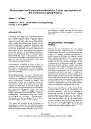
The high cost of empirical investigation in an operating steel plant makes it prudent to use all 

available tools in designing, troubleshooting and optimizing the process. Physical modeling, such 

as using water to simulate molten steel, enables significant insights into the flow behavior of liquid 

steel processes. The complexity of the continuous casting process and the phenomena which 

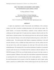
govern it, illustrated in Figs. 5.1 and 5.2, make it difficult to model. However, with the increasing 

Fig. 6.1 Schematic of continuous casting process. 

Copyright © 2003, The AISE Steel Foundation, Pittsburgh, PA. All rights reserved. 1

Casting Volume 

power of computer hardware and software, mathematical modeling is becoming an important tool 

to understand all aspects of the process. 

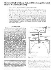
Fig. 5.2 Schematic of phenomena in the mold region of a steel slab caster. 

5.1 Physical Models 

Previous understanding of fluid flow in continuous casting has come about mainly through experiments 

using physical water models. This technique is a useful way to test and understand the 

effects of new configurations before implementing them in the process. A full-scale model has the 

important additional benefit of providing operator training and understanding. 

Construction of a physical model is based on satisfying certain similitude criteria between the 

model and actual process by matching both the geometry and the force balances that govern the 

important phenomena of interest. 1–4 Some of the forces important to flow phenomena are listed in 

Table 5.1. To reproduce the molten steel flow pattern with a water model, all of the ratios between 

2 Copyright © 2003, The AISE Steel Foundation, Pittsburgh, PA. All rights reserved.


the dominant forces must be the same in both systems. This ensures that velocity ratios between 

the model and the steel process are the same at every location. Table 5.2 shows some of the important 

force ratios in continuous casting flows, which define dimensionless groups. The size of a 

dimensionless group indicates the relative importance of two forces. Very small or very large 

groups can be ignored, but all dimensionless groups of intermediate size in the steel process must 

be matched in the physical model. 

Table 5.1 Forces Important to Fluid Flow Phenomena. 

Inertia ρ L 2 V 2 L = length scale (m) 

Gravity ρ g L 3 V = velocity (m/s) 

Buoyancy (ρ – ρp) g L 3 ρ = fluid density (kg/m 3 ) 

Viscous force µ L V µ = viscosity (kg/m-s) 

Thermal buoyancy ρ g L 3 β ∆T g = gravity accel. = 9.81 m/s 2 

Surface tension σ L σ = surface tension (N/m) 

Table 5.2 Dimensionless Groups Important to Fluid Flow Phenomena. 

Force Ratio Definition Name Phenomena 

Inertial VLρ Reynolds Fluid momentum 

Viscous µ 

Inertial V 2 

Gravitational gL 

Inertial V 2 

Thermal buoyancy gLβ∆T 

Froude Gravity-driven flow; Surface waves 

Froude* Natural convection 

Inertial ρLV 2 Weber Bubble formation; Liquid jet atomization 

Surface Tension σ 

* Modified Froude number 

β = thermal exp. coef. (m/m-°C) 

∆T = temperature difference (°C) 

p = particle of solid or gas 

An appropriate geometry scale and fluid must be chosen to achieve these matches. It is fortunate 

that water and steel have very similar kinematic viscosities (µ/ρ). Thus, Reynolds and Froude 

numbers can be matched simultaneously by constructing a full-scale water model. Satisfying these 

two criteria is sufficient to achieve reasonable accuracy in modeling isothermal single-phase flow 

systems, such as the continuous casting nozzle and mold, which has been done with great success. 

A full-scale model has the extra benefit of easy testing of plant components and operator training. 

Actually, a water model of any geometric scale produces reasonable results for most of these flow 

systems, so long as the velocities in both systems are high enough to produce fully turbulent flow 

and very high Reynolds numbers. Because flow through the tundish and mold nozzles are gravity 

driven, the Froude number is usually satisfied in any water model of these systems where the 

hydraulic heads and geometries are all scaled by the same amount. 



Physical models sometimes must satisfy heat similitude criteria. In physical flow models of steady 

flow in ladles and tundishes, for example, thermal buoyancy is large relative to the dominant inertial-driven 

flow, as indicated by the size of the modified Froude number (Froude* in Table 5.2), 

which therefore must be kept the same in the model as in the steel system. In ladles, where velocities 

are difficult to estimate, it is convenient to examine the square of the Reynolds number divided 

by the modified Froude number, which is called the Grashof number. Inertia is dominant in the 

mold, so thermal buoyancy can be ignored there. The relative magnitude of the thermal buoyancy 

forces can be matched in a full-scale hot water model, for example, by controlling temperatures 

and heat losses such that β∆T is the same in both model and caster. This is not easy, however, as 

the phenomena that govern heat losses depend on properties such as the fluid conductivity and specific 

heat and the vessel wall conductivity, which are different in the model and the steel vessel. In 

other systems, such as those involving low velocities, transients or solidification, simultaneously 

satisfying the many other similitude criteria important for heat transfer is virtually impossible. 

When physical flow models are used to study other phenomena, other force ratios must be satisfied 

in addition to those already mentioned. For the study of inclusion particle movement, for example, 

it is important to match the force ratios involving inertia, drag and buoyancy. This generates several 

other conditions to satisfy, such as matching the terminal flotation velocity, which is: 5 

V 

T 

2 

g( r-rp) dp 

= 

0 687 

18m( 1 + 0. 15Re 

) 

. 

(Eq. 5.1) 

where: 

VT = particle terminal velocity (m/s), 

ρ, ρp = liquid, particle densities (kg / m3 ), 

dp = particle diameter (m), 

µ = liquid viscosity (kg / m-s), 

g = gravity accel. = 9.81 m/s 2 , 

Re = particle Reynold’s number = ρVT dp / µ. 

In a full-scale water model, for example, 2.5-mm plastic beads with a density of 998 kg/m 3 might 

be used to simulate 100-µm 2300 kg/m 3 solid spherical inclusions in steel because they have the 

same terminal flotation velocity (equation 5.1), but are easier to visualize. 

Sometimes, it is not possible to match all of the important criteria simultaneously. For example, in 

studying two-phase flow, such as gas injection into liquid steel, new phenomena become important. 

The fluid density depends on the local gas fraction, so flow similitude requires additional 

matching of the gas fraction and its distribution. The gas fraction used in the water model must be 

increased in order to account for the roughly fivefold gas expansion that occurs when cold gas is 

injected into hot steel. Adjustments must also be made for the local pressure, which also affects 

this expansion. In addition to matching the gas fraction, the bubble size should be the same, so 

force ratios involving surface tension, such as the Weber number, should also be matched. In 

attempting to achieve this, it may be necessary to deviate from geometric similitude at the injection 

point and to wax the model surfaces to modify the contact angles, in order to control the initial 

bubble size. If gas momentum is important, such as for high gas injection rates, then the ratio 

of the gas and liquid densities must also be the same. For this, helium in water is a reasonable 

match for argon in steel. In many cases, it is extremely difficult to simultaneously match all of the 

important force ratios. To the extent that this can be approximately achieved, water modeling can 

reveal accurate insights into the real process. 

To quantify and visualize the flow, several different methods may be used. The easiest is to inject 

innocuous amounts of gas, tracer beads or dye into the flow for direct observation or photography. 


Quantitative mixing studies can measure concentration profiles of other tracers, such as dye with 

colorimetry measurement, salt solution with electrical conductivity, or acid with pH tracking. 4 For 

all of these, it is important to consider the relative densities of the tracer and the fluid. Accurate 

velocity measurements, including turbulence measurements, may be obtained with hot wire 

anemometry, 6 high-speed videography with image analysis, particle image velocimetry (PIV) 7, 8 or 

laser doppler velocimetry (LDV). 9 Depending on the phenomena of interest, other parameters may 

be measured, such as pressure and level fluctuations on the top surface. 10 

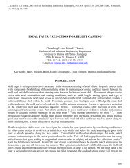
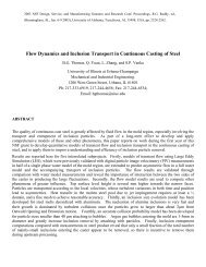
As an example, Fig. 5.3 shows the flow modeled in the mold region of a continuous thin-slab 

caster. 11 The right side visualizes the flow using dye tracer in a full-scale physical water model. 

This particular caster features a 3-port nozzle that directs some of the flow downward in order to 

stabilize the flow pattern from transient fluctuations and to dissipate some of the momentum to 

lessen surface turbulence. The symmetrical left side shows results from the other important analysis 

tool: computational modeling, which is discussed in the next section. 

5.2 Computational Models 


Fig. 5.3 Flow in a thin-slab casting mold visualized using (a) K-ε computer simulation and (b) water model with dye injection. 

From Ref. 11. 

In recent years, decreasing computational costs and the increasing power of commercial modeling 

packages are making it easier to apply mathematical models as an additional tool to understand 

complex materials processes such as the continuous casting of steel. Computational models have the 

advantage of easy extension to other phenomena such as heat transfer, particle motion and twophase 

flow, which is difficult with isothermal water models. They are also capable of more faithful 



representation of the flow conditions experienced by the steel. For example, there is no need for the 

physical bottom that interferes with the flow exiting a strand water model, and the presence of the 

moving solidifying shell can be taken into account. 

Models can now simulate most of the phenomena important to continuous casting, which include: 

fully-turbulent, transient fluid motion in a complex geometry (inlet nozzle 

and strand liquid pool), affected by argon gas bubbles, thermal and solutal 

buoyancies, 

thermodynamic reactions within and between the powder and steel phases, 

flow and heat transport within the liquid and solid flux layers, which float 

on the top surface of the steel, 

dynamic motion of the free liquid surfaces and interfaces, including the 

effects of surface tension, oscillation and gravity-induced waves, and flow 

in several phases, 

transport of superheat through the turbulent molten steel, 

transport of solute (including intermixing during a grade change), 

transport of complex-geometry inclusions through the liquid, including the 

effects of buoyancy, turbulent interactions, and possible entrapment of the 

inclusions on nozzle walls, gas bubbles, solidifying steel walls, and the top 

surface, 

thermal, fluid and mechanical interactions in the meniscus region between 

the solidifying meniscus, solid slag rim, infiltrating molten flux, liquid steel, 

powder layers and inclusion particles, 

heat transport through the solidifying steel shell, the interface between shell 

and mold (which contains powder layers and growing air gaps), and the copper 

mold, 

mass transport of powder down the gap between shell and mold, 

distortion and wear of the mold walls and support rolls, 

nucleation of solid crystals, both in the melt and against mold walls, 

solidification of the steel shell, including the growth of dendrites, grains and 

microstructures, phase transformations, precipitate formation, and 

microsegregation, 

shrinkage of the solidifying steel shell due to thermal contraction, phase 

transformations and internal stresses, 

stress generation within the solidifying steel shell due to external forces 

(mold friction, bulging between the support rolls, withdrawal, gravity), 

thermal strains, creep, and plasticity (which varies with temperature, grade 

and cooling rate), 

crack formation, 

coupled segregation, on both microscopic and macroscopic scales. 

The staggering complexity of this process makes it impossible to model all of these phenomena 

together at once. Thus, it is necessary to make reasonable assumptions and to uncouple or neglect 

the less-important phenomena. Quantitative modeling requires incorporation of all of the phenomena 

that affect the specific issue of interest, so every model needs a specific purpose. Once 

the governing equations have been chosen, they are generally discretized and solved using finitedifference 

or finite-element methods. It is important that adequate numerical validation be conducted. 

Numerical errors commonly arise from too coarse a computational domain or incomplete 

convergence when solving the nonlinear equations. Solving a known test problem and conducting 

mesh refinement studies to achieve grid independent solutions are important ways to help validate 

the model. Finally, a model must be checked against experimental measurements on both 



the laboratory and plant scales before it can be trusted to make quantitative predictions of the real 

process for a parametric study. 

5.2.1 Heat Transfer and Solidification 

Models to predict temperature and growth of the solidifying steel shell are used for basic design, 

troubleshooting and control of the continuous casting process. 12 These models solve the transient 

heat conduction equation, 

where: 

∂ 

∂ r 

∂ 

∂ ∂ 

r 

t ∂ 

∂ ∂ 

H vH 

x 

x k 

T 

x Q 

( ) + ( i ) = ( eff ) + 

i 

(Eq. 5.2) 

∂/∂t = differentiation with respect to time (s-1 ), 

ρ = density (kg/m3 ), 

H = enthalpy or heat content (J/kg), 

xi = coordinate direction, x, y or z (m), 

vi = velocity component in xi direction (m/s), 

keff = temperature-dependent effective thermal conductivity (W/m-K), 

T = temperature field (K), 

Q = heat sources (W/m3 ), 

i = coordinate direction index which, when appearing twice in a term, implies the summation 

of all three possible terms. 

An appropriate boundary condition must be provided to define heat input to every portion of the 

domain boundary, in addition to an initial condition (usually fixing temperature to the pouring temperature). 

Latent heat evolution and heat capacity are incorporated into the constitutive equation 

that must also be supplied to relate temperature with enthalpy. 

Axial heat conduction can be ignored in models of steel continuous casting because it is small relative 

to axial advection, as indicated by the small Peclet number (casting speed multiplied by shell 

thickness divided by thermal diffusivity). Thus, Lagrangian models of a horizontal slice through 

the strand have been employed with great success for steel. 13 These models drop the second term 

in equation 5.2 because velocity is zero in this reference frame. The transient term is still included, 

even if the shell is withdrawn from the bottom of the mold at a casting speed that matches the 

inflow of metal, so the process is assumed to operate at steady state. 

Heat transfer in the mold region is controlled by: 

convection of liquid superheat to the shell surface, 

solidification (latent heat evolution in the mushy zone), 

conduction through the solid shell, 

the size and properties of the interface between the shell and the mold, 

conduction through the copper mold, 

convection to the mold-cooling water. 

By far the most dominant of these is heat conduction across the interface between the surface of 

the solidifying shell and the mold, although the solid shell also becomes significant lower down. 

The greatest difficulty in accurate heat flow modeling is determination of the heat transfer across 

i 

Copyright © 2003, The AISE Steel Foundation, Pittsburgh, PA. All rights reserved. 7 

i


this gap, q gap, which varies with time and position depending on its thickness and the properties of 

the gas or lubricating flux layers that fill it: 

8 Copyright © 2003, The AISE Steel Foundation, Pittsburgh, PA. All rights reserved. 

(Eq. 5.3) 

where: 

qgap = local heat flux (W/m2 ), 

hrad = radiation heat transfer coefficient across the gap (W/m2K), kgap = effective thermal conductivity of the gap material (W/mK), 

dgap = gap thickness (m), 

T0shell = surface temperature of solidifying steel shell (K), 

T0mold = hot face surface temperature of copper mold (K). 

Usually, qgap is specified only as a function of distance down the mold, in order to match a given 

set of mold thermocouple data. 14 However, where metal shrinkage is not matched by taper of the 

mold walls, an air gap can form, especially in the corners. This greatly reduces the heat flow 

locally. More complex models simulate the mold, interface, and shell together, and use shrinkage 

models to predict the gap size. 15–17 This may allow the predictions to be more generalized. 

Mold heat flow models can feature a detailed treatment of the interface. 18–23 Some include heat, 

mass, and momentum balances on the flux in the gap and the effect of shell surface imperfections 

(oscillation marks) on heat flow and flux consumption. 23 This is useful in steel slab casting operations 

with mold flux, for example, because hrad and kgap both drop as the flux crystallizes and must 

be modeled properly in order to predict the corresponding drop in heat transfer. The coupled effect 

of flow in the molten metal on delivering superheat to the inside of the shell and thereby retarding 

solidification can also be modeled quantitatively. 23,24 Mold heat flow models can be used to identify 

deviations from normal operation and thus predict quality problems such as impending breakouts 

or surface depressions in time to take corrective action. 

During the initial fraction of a second of solidification at the meniscus, a slight undercooling of the 

liquid is required before nucleation of solid crystals can start. The nuclei rapidly grow into dendrites, 

which evolve into grains and microstructures. These phenomena can be modeled using 

microstructure models such as the cellular automata 25 and phase field26 methods. The latter 

requires coupling with the concentration field on a very small scale so is very computationally 

intensive. 

Below the mold, air mist and water spray cooling extract heat from the surface of the strand. With 

the help of model calculations, cooling rates can be designed to avoid detrimental surface temperature 

fluctuations. Online open-loop dynamic cooling models can be employed to control the spray 

flow rates in order to ensure uniform surface cooling even during transients, such as the temporary 

drop in casting speed required during a nozzle or ladle change. 27 

The strand core eventually becomes fully solidified when it reaches the “metallurgical length.” 

Heat flow models that extend below the mold are needed for basic machine design to ensure that 

the last support roll and torch cutter are positioned beyond the metallurgical length for the highest 

casting speed. A heat flow model can also be used to troubleshoot defects. For example, the location 

of a misaligned support roll that may be generating internal hot-tear cracks can be identified 

by matching the position of the start of the crack beneath the strand surface with the location of 

solidification front down the caster calculated with a calibrated model. 

5.2.2 Fluid Flow Models 

Ê k 

qgap = Á hrad 

+ 

Ë d 

gap 

gap 

ˆ 

˜ ( T0shell - T0mold) 

¯ 

Mathematical models of fluid flow can be applied to many different aspects of the continuous 

casting process, including ladles, tundishes, nozzles and molds. 12,28 A typical model solves the

following continuity equation and Navier Stokes equations for incompressible Newtonian fluids, 

which are based on conserving mass (one equation) and momentum (three equations) at every 

29, 30 

point in a computational domain: 

∂ 

+ 

∂ 

∂ 

=- 

∂ 

∂ 

+ 

∂ 

∂ P 

ruj ruiuj m 

t x 

x ∂x 

i 

i i 

∂v 

= 0 

∂x 

∂ 

+ 

∂ 

∂ Ê v u i j ˆ 

Ë 

Á ∂ ¯ 

˜ 

+ T -T 

x x 

(Eq. 5.4) 

(Eq. 5.5) 

where: 

∂/∂t = differentiation with respect to time (s-1 ), 


vi = velocity component in xi direction (m/s), 

xi = coordinate direction, x,y, or z (m), 

P = pressure field (N/m2 ), 

µ eff = effective viscosity (kg/m-s), 

T = temperature field (K), 

T0 = initial temperature (K), 

α = thermal expansion coefficient, (m/m-K), 

gj = magnitude of gravity in j direction (m/s2 ), 

Fj = other body forces (e.g., from eletromagnetic forces), 

i, j = coordinate direction indices; which when repeated in a term, implies the summation 


The second-to-last term in equation 5.5 accounts for the effect of thermal convection on the flow. 

The last term accounts for other body forces, such as due to the application of electromagnetic 

fields. The solution of these equations yields the pressure and velocity components at every point 

in the domain, which generally should be three-dimensional. At the high flow rates involved in 

these processes, these models must incorporate turbulent fluid flow. The simplest yet most computationally 

demanding way to do this is to use a fine enough grid (mesh) to capture all of the turbulent 

eddies and their motion with time. This method, known as “direct numerical simulation,” 

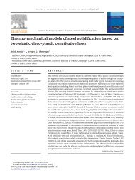
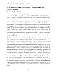
was used to produce the instantaneous velocity field in the mold cavity of a continuous steel slab 

caster shown in Fig. 5.4. 7 The 30 seconds of flow simulated to achieve these results on a 1.5 million-node 

mesh required 30 days of computation on an SGI Origin 2000 supercomputer. The calculations 

are compared with particle image velocimetry measurements of the flow in a water 

model, shown on the right side of Fig. 5.4. These calculations reveal structures in the flow pattern 

that are important to transient events such as the intermittent capture of inclusion particles. 

To achieve more computationally-efficient results, turbulence is usually modeled on a coarser grid 

using a time-averaged approximation, such as the K-ε model, 31 which averages out the effect of 

turbulence using an increased effective viscosity field, µ eff : 

meff m mtm rCm 

e 

K 

= 0 + = 0 + 

where: 

µ o , µ t = laminar and turbulent viscosity fields (kg/m-s), 

i 

i 

eff 

i 

i 

2 


a( 0 )rgj + Fj 

(Eq. 5.6) 



Fig. 5.4 Instantaneous flow pattern in a slab casting mold comparing LES simulation (left) and PIV measurement (right). 

From Ref. 7. 

ρ = fluid density (kg/m3 ), 

C µ = empirical constant = 0.09, 

K = turbulent kinetic energy field, m 2 /s2 , 

ε = turbulent dissipation field, m 2 /s3 . 

This approach requires solving two additional partial differential equations for the transport of turbulent 

kinetic energy and its dissipation: 

∂ ∂ m 

rv 

∂ ∂ s 

K Ê 

j = Á 

xj xj 

Ë 

t 

∂ 

m 

∂ 

∂ K ˆ v j Ê ∂v 

∂v 

i j ˆ 

˜ + t Á + ˜ 

x ¯ ∂xi 

Ë ∂x 

j ∂xi 

¯ 

-re 

K j 

10 Copyright © 2003, The AISE Steel Foundation, Pittsburgh, PA. All rights reserved. 

(Eq. 5.7)

where: 

∂/∂x i 

∂e ∂ m ∂e 

r 

m 

∂ ∂ s ∂ 

e Ê ˆ ∂v 

∂v 

∂v 

t 

j Ê 

i j ˆ 

v j = Á ˜ + C1 

t Á + ˜ 

xj xj Ë e xj¯ 

K ∂x 

i Ë ∂x 

j ∂xi 

¯ 

- C K 

2 

e 

re 


(Eq. 5.8) 

= differentiation with respect to coordinate direction x,y or z (m), 

K = turbulent kinetic energy field, m2 /s2 , 

ε = turbulent dissipation field, m2 /s3 , 


µ t = turbulent viscosity (kg/m-s), 

vi = velocity component in x, y or z direction (m/s), 

σK , σ × = empirical constants (1.0, 1.3), 

C1,C2 = empirical constants (1.44, 1.92), 

i, j = coordinate direction indices, which, when repeated in a term, implies the summation 


This approach generally uses special “wall functions” as the boundary conditions in order to 

achieve reasonable accuracy on a coarse grid. 31,32 Alternatively, a “low Reynold’s number” turbulence 

model can be used, which models the boundary layer in a more general way but requires a 

finer mesh at the walls. 9, 34 An intermediate method between direct numerical simulation and K-ε 

turbulence models, called “large eddy simulation,” uses a turbulence model only at the sub-grid 

scale. 35 

Most previous flow models have used the finite difference method, owing to the availability of very 

fast and efficient solution methods. 36 Popular general-purpose codes of this type include CFX, 37 

FLUENT, 38 and PHOENICS. 39 Special-purpose codes of this type include MAGMASOFT40 and 

PHYSICA, 41 which also solve for solidification and temperature evolution in castings, coupled 

with mold filling. The finite element method, such as used in FIDAP, 42 can also be applied and has 

the advantage of being more easily adapted to arbitrary geometries, although it takes longer to execute. 

Special-purpose codes of this type include PROCAST 43 and CAFE, 44 which are popular for 

investment casting processes. 

Flow in the mold is of great interest because it influences many important phenomena that have 

far-reaching consequences on strand quality. Some of these phenomena are illustrated in Fig. 5.2. 

They include the dissipation of superheat by the liquid jet impinging upon the solidifying shell 

(and temperature at the meniscus), the flow and entrainment of the top-surface powder layers, topsurface 

contour and level fluctuations, and the entrapment of subsurface inclusions and gas bubbles. 

Design compromises are needed to simultaneously satisfy the contradictory requirements for 

avoiding each of these defect mechanisms, as discussed in Chapter 14. 

It is important to extend the simulation as far upstream as necessary to provide adequate inlet 

boundary conditions for the domain of interest. For example, flow calculations in the mold should 

be preceded by calculations of flow through the submerged entry nozzle. This provides the velocities 

entering the mold in addition to the turbulence parameters, K and ε. Nozzle geometry greatly 

affects the flow in the mold and is easy to change, so it is an important subject for modeling. 

The flow pattern changes radically with increasing argon injection rate, which requires the solution 

of additional equations for the gas phase, and knowledge of the bubble size. 6,37,45 The flow pattern 

and mixing can also be altered by the application of electromagnetic forces, which can either 

brake or stir the liquid. This can be modeled by solving the Maxwell, Ohm and charge conservation 

equations for electromagnetic forces simultaneously with the flow model equations. 46 The 



great complexity that these phenomena add to the coupled model equations makes these calculations 

uncertain and a subject of ongoing research. 

5.2.3 Superheat Dissipation 

An important task of the flow pattern is to deliver molten steel to the meniscus region that has 

enough superheat during the critical first stages of solidification. Superheat is the sensible heat 

contained in the liquid metal above the liquidus temperature and is dissipated mainly in the mold. 

The transport and removal of superheat is modeled by solving equation 5.2 using the velocities 

found from the flow model (equations 5.4 to 5.8). The effective thermal conductivity of the liquid 

is proportional to the effective viscosity, which can be found from the turbulence parameters (K 

and ε). The solidification front, which forms the boundary to the liquid domain, can be treated in 

different ways. Many researchers model flow and solidification as a coupled problem on a fixed 

grid. 25,47,48 Although very flexible, this approach is subject to convergence difficulties and requires 

a fine grid to resolve the thin, 

porous mushy zone next to the 

thin shell. 

An alternative approach for 

columnar solidification of a 

thin shell, such as found in the 

mold for the continuous casting 

of steel, is to treat the 

boundary as a rough wall fixed 

at the liquidus temperature 

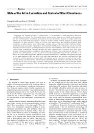
using thermal wall laws. 49 Fig. 

5.5 compares calculations using 

this approach with measured 

temperatures in the liquid pool. 50 

Incorporating the effects of 

argon on the flow pattern was 

very important in achieving the 

reasonable agreement observed. 

This figure shows that the temperature 

drops almost to the 

liquidus by mold exit, indicating 

that most of the superheat 

is dissipated in the mold. Most 

of this heat is delivered to the 

narrow face where the jet 

impinges, which is important 

to shell solidification. 51 

Fig. 5.5 Temperature distribution in mold showing superheat dissipation. From 

Ref. 50. 

The coldest regions are found 

at the meniscus at the top corners 

near the narrow face and 

near the SEN. This is a concern 

because it could lead to freezing 

of the meniscus, and 

encourage solidification of a 

thick slag rim. This could lead 

to quality problems such as 

deep oscillation marks, cracks 



and other surface defects. In the extreme, the steel surface can solidify into a solid bridge between 

the SEN and the shell against the mold wall, which often causes a breakout. To avoid these problems, 

flow must reach the surface quickly. These calculations should be used, for example, to help 

design nozzle port geometries that do not direct the flow too deep. 

5.2.4 Top Surface Powder/Flux Layer Behavior 

The flow of steel in the upper mold may influence the top surface powder layers, which are very 

important to steel quality. Mold powder is added periodically to the top surface of the steel. It sinters 

and melts to form a protective liquid flux layer, which helps to trap impurities and inclusions. 

This liquid is drawn into the gap between the shell and mold during oscillation, where it acts as a 

lubricant and helps to make heat transfer more uniform. These phenomena are difficult to measure 

or to accurately simulate with a physical model, so are worthy of mathematical modeling. 

Fig. 5.6 shows results from a 3-D finite-element model of heat transfer and fluid flow in the powder 

and flux layers, based on solving equations 5.2, 5.4 and 5.5. 52 The bottom of the model domain 

is the steel/flux interface. Its shape is imposed based on measurements in an operating caster. Alternatively, 

this interface shape can be calculated by solving additional equations to satisfy the force 

balance at the interface, which involves the pressure in the two phases, shear forces from the moving 

fluids, surface tension and gravity. 53 For the conditions in this figure, the momentum of the 

flow up the narrow face has raised the level of the interface there. The shear stress along the interface 

is determined through coupled calculations with the 3-D steady flow model. The model features 

different temperature-dependent flux properties for the interior, during sintering before 

melting, compared with the region near the narrow face mold walls, where the flux resolidifies to 

form a solid rim. 

When molten steel flows rapidly along the steel/flux interface, it induces motion in the flux layer. 

If the interface velocity becomes too high, then the liquid flux can be sheared away from the interface, 

become entrained in the steel jet, and be sent deep into the liquid pool to become trapped in 

the solidifying shell as a harmful inclusion. If the interface velocity increases further, then the interface 

standing wave becomes 

unstable, and huge level fluctuations 

contribute to further 

problems. 

The thickness of the beneficial 

liquid flux layer is also 

very important. As shown in 

the model calculations in Fig. 

5.6, the liquid flux layer may 

become dangerously thin 

near the narrow face if the 

steel flow tends to drag the 

liquid toward the center. This 

shortage of flux feeding into 

the gap can lead to air gaps, 

reduced nonuniform heat 

flow, thinning of the shell, 

and longitudinal surface 

cracks. Quantifying these 

phenomena requires modeling 

of both the steel flow and 

flux layers. 

Fig. 5.6 Comparison of measured and predicted melt-interface positions. 52 



5.2.5 Motion and Entrapment of Inclusions and Gas Bubbles 

The jets of molten steel exiting the nozzle may carry argon bubbles and inclusions such as alumina 

into the mold cavity. These particles may create defects if they become entrapped in the solidifying 

shell. Particle trajectories can be calculated using the Langrangian particle tracking method, 

which solves a transport equation for each particle as it travels through a previously-calculated 

velocity field. 34,54,55 

The force balance on each particle includes buoyancy and drag force relative to the molten steel. 

The effects of turbulent motion can be modeled crudely from a K-ε flow field by adding a random 

velocity fluctuation at each step, whose magnitude 

varies with the local turbulent kinetic energy level. To 

obtain significant statistics, the trajectories of several 

hundred individual particles should be calculated, 

using different starting points. The bubbles collect 

inclusions, and inclusion clusters collide, so their size 

and shape distributions evolve with time, which affects 

their drag and flotation velocities and importance. 

Models are being developed to include these effects. 55 

Fig. 5.7 Sample trajectories of 0.3 mm argon bubbles 

with turbulent motion. From Ref. 55. 

Fig. 5.7 shows the trajectories of several particles moving 

through a steady flow field, calculated using the Kε 

model. 55 This simulation features particle trajectory 

tracking that incorporates the influence of turbulence 

by giving a random velocity component to the velocity 

at each time step in the calculation, in proportion to the 

local turbulence level. 

Most of the argon bubbles circulate in the upper mold 

area and float out to the top surface. A few might be 

trapped at the meniscus if there is a solidification 

hook, and lead to surface defects. A few small bubbles 

manage to penetrate into the lower recirculation zone, 

where they move similarly to large inclusion clusters. 

Particles in this lower region tend to move slowly in 

large spirals, while they float toward the inner radius of the slab. When they eventually touch the 

solidifying shell in this deep region, entrapment is more likely on the inside radius. Trapped argon 

bubbles elongate during rolling and, in low-strength steel, may expand during subsequent annealing 

processes to create costly surface blisters and “pencil pipe” defects. Transient models are 

likely to yield further insights into the complex and important phenomena of inclusion entrapment. 

5.2.6 Composition Variation During Grade Changes 

Large composition differences can arise through the thickness and along the length of the final 

product due to intermixing after a change in steel grade during continuous casting. Steel producers 

need to optimize casting conditions and grade sequences to minimize the amount of steel downgraded 

or scrapped due to this intermixing. In addition, the unintentional sale of intermixed 

product must be avoided. To do this requires knowledge of the location and extent of the intermixed 

region and how it is affected by grade specifications and casting conditions. 

Models to predict intermixing must first simulate composition change in both the tundish and in 

the liquid core of the strand as a function of time. This can be done using simple lumped mixingbox 

models and/or by solving the mass diffusion equation in the flowing liquid: 


(Eq. 5.9) 

In this equation, the composition, C, ranges between the old grade concentration of 0 and the new 

grade concentration of 1. This dimensionless concept is useful because alloying elements intermix 

essentially equally, owing to the much greater importance of convection and turbulent diffusion 

Deff over laminar diffusion. In order to predict the composition distribution within the final 

product, a further model must account for the cessation of intermixing after the shell has solidified. 

Fig. 5.8 shows example composition distributions in a continuous cast slab calculated using such 

a model. 56,57 To ensure accuracy, extensive verification and calibration must be undertaken for each 

submodel. 57 The tundish mixing 

submodel must be calibrated to 

match chemical analysis of steel 

samples taken from the mold in the 

nozzle port exit streams, or with 

tracer studies using full-scale water 

models. Accuracy of a simplified 

strand submodel is demonstrated in 

Fig. 5.8 through comparison both 

with composition measurements in a 

solidified slab and with a full 3-D 

model (equation 5.4). 

The results in Fig. 5.8 clearly show 

the important difference between 

centerline and surface composition. 

New grade penetrates deeply into 

the liquid cavity and contaminates 

the old grade along the centerline. 

Old grade lingers in the tundish and 

mold cavity to contaminate the sur- 

∂ 

∂ + 

∂ 

= 

∂ 

∂ 

C 

∂ 

v 

t 

∂ ∂ 

C 

x x D 

C 

i ( eff ) 

x 

i i 

face composition of the new grade. This difference is particularly evident in small tundish, thickmold 

operations, where mixing in the strand is dominant. 

Intermix models such as this one are in use at many steel companies. The model can be enhanced to 

serve as an on-line tool by outputting, for each grade change, the critical distances that define the 

length of intermixed steel product that falls outside the given composition specifications for the old 

and new grades. 57 In addition, it can be applied off-line to perform parametric studies to evaluate the 

relative effects on the amount of intermixed steel for different intermixing operations and for different 

operating conditions using a standard ladle-exchange operation. 58 Finally, it can be used to optimize 

scheduling and casting operation in order to minimize cost. 

5.2.7 Thermal Mechanical Behavior of the Mold 

Thermal distortion of the mold during operation is important to residual stress, residual distortion, 

fatigue cracks and mold life. By affecting the internal geometry of the mold cavity, it is also important 

to heat transfer to the solidifying shell. To study thermal distortion of the mold and its related 

phenomena first requires accurate solution of heat transfer, equation 5.3, using measurements to 

help determine the interfacial heat flux. In addition, a thermal-mechanical model must solve the 

equilibrium equations that relate force and stress, the constitutive equations that relate stress and 

strain, and the compatibility equations that relate strain and displacement. 

i 


Fig. 5.8 Predicted composition distribution in a steel slab cast during a 

grade change compared with experiments. From Ref. 57. 



where: 

∂/∂x = differentiation with respect to coordinate direction (m-1 ), 

Fi = force component in i direction (N), 

σij = stress component (N/m2 ), 

xi = coordinate direction, x, y or z (m), 

= components of elasticity tensor (N/m2 ), 

Dijkl ε el 

ij 

ε tot 

ij 

ui Fi 

= 

x 

∂s 

∂ 

s = D e 

ij ijkl 

el 

ij 

tot 1 i 

eij = 2 Á 

∂x 

j 

= elastic strain component (–) 

ij 

i 

∂u 

u j 

+ 

xi 

∂ Ê ˆ 

˜ 

Ë ∂ ¯ 

(Eq. 5.10) 

(Eq. 5.11) 

(Eq. 5.12) 

= total strain component (–), 

= displacement component in i direction (m), 

i = coordinate direction index which, when appearing twice in a term, implies the 

summation of all three possible terms. 

Thermal strain is found from the temperatures 

calculated in the heat transfer model and 

accounts for the difference between the elastic 

and total strain. Further details are found 

elsewhere. 

In order to match the measured distortion, 

models should incorporate all the important 

geometric features of the mold, which often 

includes the four copper plates with their 

water slots, reinforced steel water box assemblies, 

and tightened bolts. Three-dimensional 

elastic-plastic-creep finite element models 

have been developed for slabs 59 and thin 

slabs 60,61 using the commercial finite-element 

package ABAQUS, 62 which is well suited to 

this nonlinear thermal stress problem. Their 

four-piece construction makes slab molds 

behave very differently from single-piece 

bloom or billet molds, which have also been 

studied using thermal stress models. 63 

Fig. 5.9 Distorted shape of thin slab casting mold during 

operation (50X magnification) with temperature contours 

(°C). From Ref. 61. 

Fig. 5.9 illustrates typical temperature contours 

and the displaced shape calculated in 

one quarter of the mold under steady operating 

conditions. 61 The hot exterior of each copper 

plate attempts to expand but is 

constrained by its colder interior and the cold, 



stiff, steel water jacket. This makes each plate bend in toward the solidifying steel. Maximum 

inward distortions of more than one millimeter are predicted just above the center of the mold 

faces, and below the location of highest temperature, which is found just below the meniscus. 

The narrow face is free to rotate away from the wide face and contact only along a thin vertical 

line at the front corner of the hot face. This hot edge must transmit all of the clamping forces, so 

it is prone to accelerated wear and crushing, especially during automatic width changes. If steel 

enters the gaps formed by this mechanism, this can lead to finning defects or even a sticker breakout. 

In addition, the wide faces may be gouged, leading to longitudinal cracks and other surface 

defects. 

The high compressive stress due to constrained thermal expansion induces creep in the hot exterior 

of the copper plates that face the steel. This relaxes the stresses during operation but allows 

residual tensile stress to develop during cooling. Over time, these cyclic thermal stresses and creep 

build up significant distortion of the mold plates. This can contribute greatly to remachining 

requirements and reduced mold life. Under adverse conditions, this stress could lead to cracking 

of the copper plates. The distortion predictions are important for designing mold taper to avoid 

detrimental air gap formation. 

These practical concerns can be investigated with quantitative modeling studies of the effects of 

different process and mold design variables on mold temperature, distortion, creep and residual 

stress. This type of stress model application will become more important in the future to optimize 

the design of the new molds being developed for continuous thin-slab and strip casting. For example, 

thermal distortion of the rolls during operation of a twin-roll strip caster is on the same order 

as the section thickness of the steel product. 

5.2.8 Thermal Mechanical Behavior of the Shell 

The solidifying shell is prone to a variety of distortion, cracking and segregation problems, owing 

to its creep at elevated temperature, combined with metallurgical embrittlement and thermal stress. 

To start to investigate these problems, models are being developed to simulate coupled fluid flow, 

thermal and mechanical behavior of the solidifying steel shell during continuous casting. 17,60,64 The 

thermal-mechanical solution procedure is documented elsewhere. 65 In addition to solving equations 

5.2, 5.3, 5.10, 5.11 and 5.12, further constitutive equations are needed to characterize the 

inelastic creep and plastic strains as a function of stress, temperature and structure in order to accurately 

incorporate the mechanical properties of the material. For example, 66 

̇e 

Ê -Qˆ 

ne 

p= 

C exp [ s a e ep] 

Ë 

Á 

T ¯ 

˜ - 

where: 

ε . 

= inelastic strain rate (s –1 ), 

σ = stress (MPa), 

εp = inelastic strain (structure parameter), 

T = temperature (K), 

C,Q,a ε ,n ε ,n = empirical constants. 

(Eq. 5.13) 

Constitutive equations such as these are a subject of ongoing research because the equations are 

difficult to develop, especially for complex loading conditions involving stress reversals. The 

numerical methods to evaluate them are prone to instability, and the experimental measurements 

they are based upon are difficult to conduct. 

Copyright © 2003, The AISE Steel Foundation, Pittsburgh, PA. All rights reserved. 17 

n


Thermal-mechanical models can be applied in order to predict the evolution of temperature, stress 

and deformation of the solidifying shell while in the mold for both billets 15 and slabs. 16,67–70 In this 

region, these phenomena are intimately coupled because the shrinkage of the shell affects heat 

transfer across the air gap, which complicates the calculation procedure. The predicted temperature 

contours and distorted shape of a transverse region near the corner are compared in Fig. 5.10 

with measurements of a breakout shell from an operating steel caster. 16 This model tracks the 

behavior of a two-dimensional 

slice through the 

strand as it moves downward 

at the casting speed 

through the mold and 

upper spray zones. It 

consists of separate 

finite-element models of 

heat flow and stress generation 

that are step-wise 

coupled through the size 

of the interfacial gap. 

The heat transfer model 

was calibrated using 

thermocouple measurements 

down the centerline 

of the wide face for 

typical conditions. 

Fig. 5.10 Comparison between predicted and measured shell thickness in a horizontal 

(x-y) section through the corner of a continuous-cast steel breakout shell. From Ref. 16. 

Shrinkage predictions 

from the stress model are 

used to find the air gap 

thickness needed in equation 5.3 in order to extend the calculations around the mold perimeter. The 

model includes the effect of mold distortion on the air gaps, and superheat delivery from the flowing 

jet of steel, calculated in separate models. The stress model includes ferrostatic pressure from 

the molten steel on the inside of the shell and calculates intermittent contact between the shell and 

the mold. It also features a temperature-dependent elastic modulus and an elastic-viscoplastic constitutive 

equation that includes the effects of temperature, composition, phase transformations and 

stress state on the local inelastic creep rate. Efficient numerical algorithms are needed to integrate 

the equations. 

As expected, good agreement is obtained in the region of good contact along the wide face, where 

calibration was done. Near the corner along the narrow face, steel shrinkage is seen to exceed the 

mold taper, which was insufficient. Thus, an air gap is predicted. This air gap lowers heat extraction 

from the shell in the off-corner region of the narrow face. When combined with high superheat 

delivery from the bifurcated nozzle directed at this location, shell growth is greatly reduced 

locally. Just below the mold, this thin region along the off-corner narrow-face shell caused the 

breakout. 

Near the center of the narrow face, creep of the shell under ferrostatic pressure from the liquid is 

seen to maintain contact with the mold, so much less thinning is observed. This illustrates the 

tremendous effect that superheat has on slowing shell growth, if there is a problem that lowers heat 

flow. 

Fig. 5.11 presents sample distributions of temperature and stress through the thickness of the shell, 

calculated with this model. 70 To achieve reasonable accuracy, a very fine mesh and small time steps 

are needed. The temperature profile is almost linear through the shell. The stress profile shows that 

the shell surface is in compression. This is because, in the absence of friction with the mold, the 

surface layer solidifies and cools stress free. As each inner layer solidifies, it cools and tries to shrink, 


while the surface temperature 

remains relatively constant. 

The slab is constrained to 

remain planar, so complementary 

subsurface tension and 

surface compression stresses 

are produced. Note that the 

average stress through the shell 

thickness is zero in order to 

maintain force equilibrium. It 

is significant that the maximum 

tensile stress is found 

near the solidification front. 

This generic subsurface tensile 

stress is responsible for hot 

tear cracks, when accompanied 

by metallurgical embrittlement. 

Thermal-mechanical models such as this one can be applied to predict ideal mold taper, 71 to prevent 

breakouts such as the one discussed here 24 and to understand the cause of other problems such 

as surface depressions 72 and longitudinal cracks. When combined with transient temperature, flow 

and pressure calculations in the slag layers, such models can simulate phenomena at the meniscus 

such as oscillation mark formation. 73 

Computational models can also be applied to calculate thermomechanical behavior of the solidifying 

shell below the mold. Models can investigate shell bulging between the support rolls due to 

ferrostatic-pressure induced creep, 74–78 and the stresses induced during unbending. 79 These models 

are important for the design of spray systems and rolls in order to avoid internal hot tear cracks and 

centerline segregation. These models face great numerical challenges because the phenomena are 

generally three-dimensional and transient, the constitutive equations are highly nonlinear, and the 

mechanical behavior in one region (e.g., the mold) may be coupled with the behavior very far away 

(e.g., unbending rolls). 

5.2.9 Crack Formation 


Fig. 5.11 Typical temperature and stress distributions through shell thickness. 

From Ref. 70. 

Although obviously of great interest, crack formation is particularly difficult to model directly and 

is rarely attempted. Very small strains (on the order of 1%) can start hot tear cracks at the grain 

boundaries if liquid metal is unable to feed through the secondary dendrite arms to accommodate 

the shrinkage. Strain localization may occur on both the small scale (when residual elements segregate 

to the grain boundaries) and on a larger scale (within surface depressions or hot spots). Later 

sources of tensile stress, including constraint due to friction and sticking, unsteady cooling below 

the mold, withdrawal forces, bulging between support rolls, and unbending all worsen strain concentration 

and promote crack growth. Microstructure, grain size and segregation are extremely 

complex, so modeling of these phenomena is generally done independently of the stress model. Of 

even greater difficulty for computational modeling is the great difference in scale between these 

microstructural phenomena relative to the size of the casting, where the important macroscopic 

temperature and stress fields develop. 

Considering this complexity, the results of macroscopic thermal-stress models are linked to the 

microstructural phenomena that control crack initiation and propagation through the use of fracture 

criteria. To predict hot tear cracks, most fracture criteria identify a critical amount of inelastic 

strain (e.g., 1 – 3.8%) accumulated over a critical range of liquid fraction, fL , such as 0.01< fL < 

0.2. 80,81 Recent work suggests that the fracture criteria should consider the inelastic strain rate, 



which is important during liquid feeding through a permeable region of dendrite arms in the mushy 

zone. 82 Careful experiments are needed to develop these fracture criteria by applying stress during 

solidification. 83–85 There experiments are difficult to control, so detailed modeling of the experiment 

itself is becoming necessary, in order to extract more fundamental material properties such 

as fracture criteria. 

5.2.10 Centerline Segregation 

Macrosegregation near the centerline of the solidified slab is detrimental to product properties, particularly 

for highly alloyed steels, which experience the most segregation. Centerline segregation 

can be reduced and even avoided through careful application of electromagnetic forces, and soft 

reduction, where the slab is rolled or quenched just before it is fully solidified. Computational 

modeling would be useful to understanding and optimizing these practices. 

Centerline segregation is a very difficult problem to simulate because such a wide range of coupled 

phenomena must be properly modeled. Bulging between the rolls and solidification shrinkage 

together drive the fluid flow necessary for macrosegregation, so fluid flow, solidification heat 

transfer and stresses must all be modeled accurately (including equations 5.2, 5.4, 5.5, 5.10, 5.12 

and 5.13). The microstructure is also important, as equiaxed crystals behave differently than 

columnar grains, and so must also be modeled. This is complicated by the convection of crystals in 

the molten pool in the strand, which depends on both flow from the nozzle and thermal/solutal convection. 

Increasing superheat tends to worsen segregation, so the details of mold superheat transfer 

must also be properly modeled. Naturally, equation 5.8 must be solved for each important alloying 

element on both the microstructural scale (between dendrite arms), with the help of microsegregation 

software such as THERMOCALC, 86 and on the macroscopic scale (from surface to center of 

the strand), using advanced computations. 48,87 The diffusion coefficients and partition coefficients 

needed for this calculation are not currently known with sufficient accuracy. Finally, the application 

of electromagnetic and roll forces generate additional modeling complexity. Although the task 

appears overwhelming, steps are being taken to model this important problem. 88,89 

Much further work is needed to understand and quantify these phenomena and to apply the results 

to optimize the continuous casting process. In striving towards these goals, the importance of combining 

modeling and experiments together cannot be overemphasized. 

5.3 Conclusion 

The final test of a model is if the results can be implemented and improvements can be achieved, 

such as the avoidance of defects in the steel product. Plant trials are ultimately needed for this 

implementation. Trials should be conducted on the basis of insights supplied from all available 

sources, including physical models, mathematical models, literature and previous experience. 

As increasing computational power continues to advance the capabilities of numerical simulation 

tools, modeling should play an increasing role in future advances to high-technology processes 

such as the continuous casting of steel. Modeling can augment traditional research methods in generating 

and quantifying the understanding needed to improve any aspect of the process. Areas 

where advanced computational modeling should play a crucial role in future improvements include 

transient flow simulation, mold flux behavior, taper design, online quality prediction and control, 

especially for new problems and processes such as high-speed billet casting, thin slab casting and 

strip casting. 

Future advances in the continuous casting process will not come from either models, experiments, 

or plant trials. They will come from ideas generated by people who understand the process and the 



problems. This understanding is rooted in knowledge, which can be confirmed, deepened, and 

quantified by tools that include computational models. As our computational tools continue to 

improve, they should grow in importance in fulfilling this important role, leading to future process 

advances. 

References 

1. J. Szekely, J.W. Evans and J.K. Brimacombe, The Mathematical and Physical Modeling of Primary 

Metals Processing Operations (New York: John Wiley & Sons, 1987). 

2. J. Szekely and N. Themelis, Rate Phenomena in Process Metallurgy (New York: Wiley-Interscience, 

1971), 515–597. 

3. R.I.L. Guthrie, Engineering in Process Metallurgy (Oxford, UK: Clarendon Press, 1992), 528. 

4. L.J. Heaslip and J. Schade, “Physical Modeling and Visualization of Liquid Steel Flow Behavior 

During Continuous Casting,” Iron & Steelmaker, 26:1 (1999): 33–41. 

5. S.L. Lee, “Particle Drag in a Dilute Turbulent Two-Phase Suspension Flow,” Journal of Multiphase 

Flow, 13:2 (1987): 247. 

6. B.G. Thomas, X. Huang and R.C. Sussman, “Simulation of Argon Gas Flow Effects in a Continuous 

Slab Caster,” Metall. Trans. B, 25B:4 (1994): 527–547. 

7. S. Sivaramakrishnan, H. Bai, B.G. Thomas, P. Vanka, P. Dauby and M. Assar, “Transient Flow 

Structures in Continuous Cast Steel,” in Ironmaking Conference Proceedings, 59, Pittsburgh, 

Pa. (Warrendale, Pa.: Iron and Steel Society, 2000), 541–557. 

8. M.B. Assar, P.H. Dauby and G.D. Lawson, “Opening the Black Box: PIV and MFC Measurements 

in a Continuous Caster Mold,” in Steelmaking Conference Proceedings, 83 (Warrendale, 

Pa.: Iron and Steel Society, 2000), 397–411. 

9. X.K. Lan, J.M. Khodadadi and F. Shen, “Evaluation of Six k-Turbulence Model Predictions of 

Flowin a Continuous Casting Billet-Mold Water Model Using Laser Doppler Velocimetry 

Measurements,” Metall. Mater. Trans., 28B:2 (1997): 321–332. 

10. J. Herbertson, Q.L. He, P.J. Flint and R.B. Mahapatra, “Modelling of Metal Delivery to Continuous 

Casting Moulds,” in Steelmaking Conference Proceedings, 74 (Warrendale, Pa.: Iron 

and Steel Society, 1991), 171–185. 

11. B.G. Thomas, R. O’Malley, T. Shi, Y. Meng, D. Creech and D. Stone, “Validation of Fluid 

Flow and Solidification Simulation of a Continuous Thin Slab Caster,” in Modeling of Casting, 

Welding, and Advanced Solidification Processes, IX, Aachen, Germany, Aug. 20–25, 2000 

(Aachen, Germany: Shaker Verlag GmbH, 2000), 769–776. 

12. B.G. Thomas, “Mathematical Modeling of the Continuous Slab Casting Mold: A State of the 

Art Review,” in 74th Steelmaking Conference Proceedings, 74 (Warrendale, Pa.: Iron and Steel 

Society, 1991), 105–118. 

13. J. Lait, J.K. Brimacombe and F. Weinberg, “Mathematical Modelling of Heat Flow in the Continuous 

Casting of Steel,” Ironmaking and Steelmaking, 2 (1974): 90–98. 

14. R.B. Mahapatra, J.K. Brimacombe and I.V. Samarasekera, “Mold Behavior and its Influence 

on Quality in the Continuous Casting of Slabs: Part I. Industiral Trials, Mold Temperature 

Measurements, and Mathematical Modelling,” Metallurgical Transactions B, 22B (Dec. 

(1991), 861–874. 

15. J.E. Kelly, K.P. Michalek, T.G. OConnor, B.G. Thomas, J.A. Dantzig, “Initial Development of 

Thermal and Stress Fields in Continuously Cast Steel Billets,” Metallurgical Transactions A, 

19A:10 (1988): 2589–2602. 

16. A. Moitra and B.G. Thomas, “Application of a Thermo-Mechanical Finite Element Model of 

Steel Shell Behavior in the Continuous Slab Casting Mold,” in Steelmaking Proceedings, 76 

(Dallas, Texas: Iron and Steel Society, 1993), 657–667. 

17. J.-E. Lee, T.-J. Yeo, K.H. Oh, J.-K. Yoon and U.-S. Yoon, “Prediction of Cracks in Continuously 

Cast Beam Blank Through Fully Coupled Analysis of Fluid Flow, Heat Transfer and 

Deformation Behavior of Solidifying Shell,” Metall. Mater. Trans. A, 31A:1 (2000): 

225–237. 



18. R. Bommaraju and E. Saad, “Mathematical modelling of lubrication capacity of mold fluxes,” 

in Steelmaking Proceedings, 73 (Warrendale, Pa.: Iron and Steel Society, 1990), 281–296. 

19. B.G. Thomas and B. Ho, “Spread Sheet Model of Continuous Casting,” J. Engineering Industry, 

118:1 (1996): 37–44. 

20. B. Ho, “Characterization of Interfacial Heat Transfer in the Continuous Slab Casting Process” 

(Masters Thesis, University of Illinois at Urbana–Champaign, 1992). 

21. J.A. DiLellio and G.W. Young, “An Asymptotic Model of the Mold Region in a Continuous 

Steel Caster,” Metall. Mater. Trans., 26B:6 (1995): 1225–1241. 

22. B.G. Thomas, D. Lui and B. Ho, “Effect of Transverse and Oscillation Marks on Heat Transfer 

in the Continuous Casting Mold,” in Applications of Sensors in Materials Processing, 

edited by V. Viswanathan, Orlando, Fla. (Warrendale, Pa.: TMS, 1997), 117–142. 

23. B.G. Thomas, B. Ho and G. Li, “Heat Flow Model of the Continuous Slab Casting Mold, Interface, 

and Shell,” in Alex McLean Symposium Proceedings, Toronto (Warrendale, Pa.: Iron and 

Steel Society, 1998), 177–193. 

24. G.D. Lawson, S.C. Sander, W.H. Emling, A. Moitra and B.G. Thomas, “Prevention of Shell 

Thinning Breakouts Associated with Widening Width Changes,” in Steelmaking Conference 

Proceedings, 77 (Warrendale, Pa.: Iron and Steel Society, 1994), 329–336. 

25. C.-A. Gandin, T. Jalanti and M. Rappaz, “Modeling of Dendritic Grain Structures,” in Modeling 

of Casting, Welding, and Advanced Solidification Processes, VIII, edited by B.G. Thomas 

and C. Beckermann (Warrendale, Pa.: TMS, 1998), 363–374. 

26. I. Steinbach and G.J. Schmitz, “Direct Numerical Simulation of Solidification Structure using 

the Phase Field Method,” in Modeling of Casting, Welding, and Advanced Solidification 

Processes, VIII, edited by B.G. Thomas and C. Beckermann (Warrendale, Pa.: TMS, 1998), 

521–532. 

27. R.A. Hardin, K. Liu and C. Beckermann, “Development of a Model for Transient Simulation 

and Control of a Continuous Steel Slab Caster,” in Materials Processing in the Computer Age, 

3 (Warrendale, Pa.: Minerals, Metals, & Materials Society, 2000), 61–74. 

28. J. Szekely and R.T. Yadoya, “The Physical and Mathematical Modelling of the Flow Field in 

teh Mold Region of Continuous Casitng Units. Part II. Computer Solution of the Turbulent 

Flow Equations,” Metall. Mater. Trans., 4 (1973): 1379. 

29. S.V. Patankar, Numerical Heat Transfer and Fluid Flow (New York: McGraw Hill, 1980). 

30. S.V. Patankar and B.D. Spalding, “A calculation procedure for heat, mass and momentum 

transer in three-dimensional parabolic flows,” Int. J. Heat Mass Transfer, 15 (1992): 1787- 

1806. 

31. B.E. Launder and D.B. Spalding, “Numerical Computation of Turbulent Flows,” Computer 

Methods in Applied Mechanics and Engr, 13 (1974): 269–289. 

32. B.G. Thomas and F.M. Najjar, “Finite-Element Modeling of Turbulent Fluid Flow and Heat 

Transfer in Continuous Casting,” Applied Mathematical Modeling, 15 (1991): 226–243. 

33. D.E. Hershey, B.G. Thomas and F.M. Najjar, “Turbulent Flow through Bifurcated Nozzles,” 

International Journal for Numerical Methods in Fluids, 17 (1993): 23–47. 

34. M.R. Aboutalebi, M. Hasan and R.I.L. Guthrie, “Coupled Turbulent Flow, Heat, and Solute 

Transport in Continuous Casting Processes,” Metall. Mater. Trans., 26B:4 (1995): 731–744. 

35. J. Smagorinsky, “General Circulation Experiments with the Primitive Equations” (Washington: 

Report, Weather Bureau, 1963), 99–121. 

36. N.C. Markatos, “Computational Fluid Flow Capabilities and Software,” Ironmaking and Steelmaking, 

16:4 (1989): 266–273. 

37. “CFX 4.2” (Pittsburgh, Pa.: AEA Technology, 1998). 

38. “FLUENT 5.1” (Lebanon, N.H.: Fluent Inc., 2000). 

39. “PHOENICS” (London: CHAM, 2000). 

40. E. Flender, “MAGMASOFT” (Aachen, Germany: Magma Gmbh, 2000). 

41. M. Cross, “PHYSICA” (Greenwich, UK: Computing & Math Sciences, 2000). 

42. M.S. Engleman, “FIDAP 8.5” (Evanston, Ill.: Fluent, Inc., 2000). 

43. M. Sammonds, “PROCAST” (Annapolis, Md.: UES Software, 2000). 

44. P. Thevoz, “CAFE” (Lausanne, Switzerland: CALCOM, EPFL, 2000). 



45. N. Bessho, R. Yoda, H. Yamasaki, T. Fujii and T. Nozaki, “Numerical Analysis of Fluid Flow 

in the Continuous Casting Mold by a Bubble Dispersion Model,” Iron and Steelmaker, 18:4 

(1991): 39–44. 

46. T. Ishii, S.S. Sazhin and M. Makhlouf, “Numerical prediction of magnetohydrodynamic flow 

in continuous casting process,” Ironmaking and Steelmaking, 23:3 (1996): 267–272. 

47. V.R. Voller, A.D. Brent and C. Prakash, “The Modelling of Heat, Mass and Solute Transport 

in Solidification Systems,” Applied Mathematical Modelling, 32 (1989): 1719–1731. 

48. M.C. Schneider and C. Beckermann, “The Formation of Macrosegregation by Multicomponent 

Thermosolutal Convection During the Solidification of Steel,” Metall. Mater. Trans. A, 

26A (1995): 2373–2388. 

49. X. Huang, B.G. Thomas and F.M. Najjar, “Modeling Superheat Removal During Continuous 

Casting of Steel Slabs,” Metallurgical Transactions B, 23B:6 (1992): 339–356. 

50. B.G. Thomas, “Continuous Casting of Steel, Chap. 15,” in Modeling and Simulation for Casting 

and Solidification: Theory and Applications, edited by O. Yu (New York: Marcel Dekker, 2000). 

51. H. Nakato, M. Ozawa, K. Kinoshita, Y. Habu and T. Emi, “Factors Affecting the Formation of 

Shell and Longitudinal Cracks in Mold During High-Speed Continuous Casting of Slabs,” 

Trans. Iron Steel Inst. Japan, 24:11 (1984): 957–965. 

52. R. McDavid and B.G. Thomas, “Flow and Thermal Behavior of the Top-Surface Flux/Powder 

Layers in Continuous Casting Molds,” Metallurgical Transactions B, 27B:4 (1996): 672–685. 

53. G.A. Panaras, A. Theodorakakos and G. Bergeles, “Numerical Investigation of the Free Surface 

in a continuous Steel Casting Mold Model,” Metall. Mater. Trans. B, 29B (5) (1998): 1117–1126. 

54. R.C. Sussman, M. Burns, X. Huang and B.G. Thomas, “Inclusion Particle Behavior in a Continuous 

Slab Casting Mold,” in 10th Process Technology Conference Proc., 10, Toronto (Warrendale, 

Pa.: Iron and Steel Society, 1992), 291–304. 

55. B.G. Thomas, A. Dennisov and H. Bai, “Behavior of Argon Bubbles During Continuous Casting 

of Steel,” in Steelmaking Conference Proceedings, 80, Chicaago (Warrendale, Pa.: Iron and 

Steel Society, 1997), 375–384. 

56. X. Huang and B.G. Thomas, “Modeling of Steel Grade Transition in Continuous Slab Casting 

Processes,” Metallurgical Transactions, 24B (1993): 379–393. 

57. X. Huang and B.G. Thomas, “Intermixing Model of Continuous Casting During a Grade Transition,” 

Metallurgical Mater Transactions B, 27B:4 (1996): 617–632. 

58. B.G. Thomas, “Modeling Study of Intermixing in Tundish and Strand During a Continuous- 

Casting Grade Transition,” ISS Transactions, 24:12 (1997): 83–96. 

59. B.G. Thomas, G. Li, A. Moitra and D. Habing, “Analysis of Thermal and Mechanical Behavior 

of Copper Molds during Continuous Casting of Steel Slabs,” Iron and Steelmaker (ISS 

Transactions), 25:10 (1998): 125–143. 

60. T. O’Conner and J. Dantzig, “Modeling the Thin Slab Continuous Casting Mold,” Metall. 

Mater. Trans., 25B:4 (1994): 443–457. 

61. J.-K. Park, I.V. Samarasekera, B.G. Thomas and U.-S. Yoon, “Analysis of Thermal and 

Mechanical Behavior of Copper Mould During Thin Slab Casting,” in Steelmaking Conference 

Proceedings, 83 (Warrendale, Pa.: Iron and Steel Society, 2000), 9–21. 

62. “ABAQUS 5.8” (Pawtucket, R.I.: Hibbitt, Karlsson & Sorensen, Inc., 1999). 

63. I.V. Samarasekera, D.L. Anderson and J.K. Brimacombe, “The Thermal Distortion of Continuous 

Casting Billet Molds,” Metallurgical Transactions B, 13B (March 1982): 91–104. 

64. A. Cristallini, M.R. Ridolfi, A. Spaccarotella, R. Capotosti, G. Flemming and J. Sucker, 

“Advanced Process Modeling of CSP Funnel Design for Thin Slab Casting of High-Alloyed 

Steels,” in Seminario de Aceria of the Instituto Argentino de Siderurgia (IAS) Proceedings, 

(Buones Aires, Argentina: IAS, 1999), 468–477. 

65. J.A. Dantzig, “Thermal Stress Development in Metal Casting Processes,” Metallurgical Science 

and Technology, 7:3 (1989): 133–178. 

66. P. Kozlowski, B.G. Thomas, J. Azzi and H. Wang, “Simple Constitutive Equations for Steel at 

High Temperature,” Metallurgical Transactions A, 23A (March 1992): 903–918. 

67. K. Sorimachi and J.K. Brimacombe, “Improvements in Mathematical Modelling of Stresses in 

Continuous Casting of Steel,” Ironmaking and Steelmaking, 4 (1977): 240–245. 



68. K. Kinoshita, H. Kitaoka and T. Emi, “Influence of Casting Conditions on the Solidification of 

Steel Melt in Continuous Casting Mold,” Tetsu-to-Hagane, 67:1 (1981): 93–102. 

69. I. Ohnaka and Y. Yashima, “Stress Analysis of Steel Shell Solidifying in Continuous Casting 

Mold,” in Modeling of Casting and Welding Processes IV, 4 (Warrendale, Pa.: Minerals, Metals, 

and Materials Society, 1988), 385–394. 

70. B.G. Thomas and J.T. Parkman, “Simulation of Thermal Mechanical Behavior During Initial 

Solidification,” in Thermec 97 Internat. Conf. on Thermomechanical Processing of Steel and 

Other Materials, 2, edited by T. Chandra (Wollongong, Australia: TMS, 1997), 2279–2285. 

71. B.G. Thomas, A. Moitra and W.R. Storkman, “Optimizing Taper in Continuous Slab Casting 

Molds Using Mathematical Models,” in Proceedings, 6th International Iron and Steel Congress, 

3, Nagoya, Japan (Tokyo: Iron & Steel Inst. Japan, 1990), 348–355. 

72. B.G. Thomas, A. Moitra and R. McDavid, “Simulation of Longitudinal Off-Corner Depressions 

in Continuously-Cast Steel Slabs,” ISS Transactions, 23:4 (1996): 57–70. 

73. K. Schwerdtfeger and H. Sha, “Depth of Oscillation Marks Forming in Continuous Casting of 

Steel,” Metallurgical and Materials Transactions A, in press (1999). 

74. A. Palmaers, A. Etienne and J. Mignon, “Calculation of the Mechanical and Thermal Stresses 

in Continuously Cast Strands, in German,” Stahl und Eisen, 99:19 (1979): 1039–1050. 

75. J.B. Dalin and J.L. Chenot, “Finite Element Computation of Bulging in Continuously Cast 

Steel with a Viscoplastic Model,” International Journal for Numerical Methods in Engineering, 

25 (1988): 147–163. 

76. B. Barber and A. Perkins, “Strand Deformation in Continuous Casting,” Ironmaking and Steelmaking, 

16:6 (1989): 406–411. 

77. K. Okamura and H. Kawashima, “Calculation of Bulging Strain and Its Application to Prediction 

of Internal Cracks in Continuously Cast Slabs,” in Proc. Int. Conf. Comp. Ass. Mat. Design 

Proc. Simul. (Tokyo: ISIJ, 1993), 129–134. 

78. L. Yu, “Bulging in Continuous Cast Steel Slabs” (M.S. Thesis, University of Illinois, 2000). 

79. M. Uehara, I.V. Samarasekera and J.K. Brimacombe, “Mathematical modelling fo unbending 

of continuously cast steel slabs,” Ironmaking and Steelmaking, 13:3 (1986), 138. 

80. T.W. Clyne and G.J. Davies, “The influence of composition on solidification cracking susceptibiltity 

in binary alloy systems,” Br. Foundrymen, 74:4 (1981): 65–73. 

81. A. Yamanaka, K. Nakajima and K. Okamura, “Critical strain for internal crack formation in 

continuous casting,” Ironmaking and Steelmaking, 22:6 (1995): 508–512. 

82. M. Rappaz, J.-M. Drezet and M. Gremaud, “A New Hot-Tearing Criterion,” Metall. Mater. 

Trans. A, 30A:2 (1999): 449–455. 

83. T. Matsumiya, M. Ito, H. Kajioka, S. Yamaguchi, Y. Nakamura, “An Evaluation of Critical 

Strain for Internal Crack Formation in Continuously Cast Slabs,” Transactions of the Iron and 

Steel Institute of Japan, 26 (1986): 540–546. 

84. C. Bernhard, H. Hiebler and M.M. Wolf, “Experimental simulation of subsurface crack formation 

in continuous casting,” Rev. Metall. (March 2000), 333–344. 

85. C.H. Yu, M. Suzuki, H. Shibata, T. Emi, “Simulation of Crack Formation on Solidifying Steel 

Sheel in Continuous Casting Mold,” ISIJ International, 36 (1996): S159–S162. 

86. B. Sundman, B. Jansson and J.O. Anderson, “The Thermo-Calc Databank System,” CAL- 

PHAD 9, 2 (1985): 153–190. 

87. C.Y. Wang and C. Beckermann, “Equiaxed Dendritic Solidification with Convection,” Metall. 

Mater. Trans. A, 27A:9 (1996): 2754–2764. 

88. T. Kajitani, J.-M. Drezet and M. Rappaz, “Numerical simulation of deformation-induced segregation 

in continuous casting of steel,” Metall. Mater. Trans. (2001), in press. 

89. G. Lesoult and S. Sella, Solid State Phenomena, 3 (1988): 167–178.

a PDF version - Continuous Casting Consortium - University of ...

Create successful ePaper yourself

Delete template?

Save as template?