Cost Benefit Analysis of Washington-Richmond High-Speed Rail
Cost Benefit Analysis of Washington-Richmond High-Speed Rail
Cost Benefit Analysis of Washington-Richmond High-Speed Rail

Create successful ePaper yourself
Turn your PDF publications into a flip-book with our unique Google optimized e-Paper software.
Spring<br />
2010<br />
<strong>Cost</strong>-<strong>Benefit</strong> <strong>Analysis</strong> <strong>of</strong> <strong>Washington</strong>-<br />
<strong>Richmond</strong> <strong>High</strong>-<strong>Speed</strong> <strong>Rail</strong><br />
Prepared By:<br />
For:<br />
George Mason University:<br />
PUBP 722:<br />
School <strong>of</strong> Public Policy<br />
Transportation Policy, Operations<br />
and Logistics Practicum<br />
Published May 14, 2010
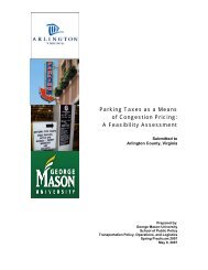
<strong>Cost</strong> <strong>Benefit</strong> <strong>Analysis</strong> <strong>of</strong> <strong>Washington</strong>-<strong>Richmond</strong> <strong>High</strong>-<strong>Speed</strong> <strong>Rail</strong> Spring 2010<br />
Cover image: Amtrak train number 91, Silver Star departing <strong>Washington</strong> D.C. en route to Miami, Florida.<br />
Photograph by: S. Moskowitz, May 12, 2010<br />
This report is prepared by the students <strong>of</strong> the 2010 Transportation Policy Operations and Logistics<br />
Practicum (PUBP 722) under guidance from Dr. Laurie Schintler.<br />
Faculty Advisor: Dr. Laurie Schintler<br />
Project Leads: Heather Hamilton; Jeffery Sangillo<br />
Class Roster:<br />
• Gretchen Bronson<br />
• Paul Chang<br />
• Daniel Favarulo<br />
• Alberto Fernandez Oviedo<br />
• Jeremy Flores<br />
• Dustin Gamache<br />
• Kai Li<br />
• Robert Mariner<br />
• Philip Mayer<br />
2<br />
• Matthew Miller<br />
• Garry Moore<br />
• Stephen Moskowitz<br />
• Donna Norfleet<br />
• Paul Sarahan<br />
• Nansak Shagaya<br />
• Benjamin Thielen<br />
• Joseph Winterer
<strong>Cost</strong> <strong>Benefit</strong> <strong>Analysis</strong> <strong>of</strong> <strong>Washington</strong>-<strong>Richmond</strong> <strong>High</strong>-<strong>Speed</strong> <strong>Rail</strong> Spring 2010<br />
Acknowledgements<br />
The Transportation Policy Operations and Logistics Spring Practicum 2010 would like to thank the<br />
following people that contributed to the report with expertise and data that we could not have<br />
produced our results without:<br />
3<br />
• Edgar Courtemanch, Amtrak<br />
• Jeff Mann, Amtrak<br />
• Bruce T. Williams, AECOM Transportation<br />
• Kevin Page, Virginia Department <strong>of</strong> <strong>Rail</strong> and Public Transportation<br />
• T. Ross Hudnall, Virginia Department <strong>of</strong> Transportation<br />
• Zhenhau Chen, PhD Candidate, George Mason University<br />
• Jack Wells, Chief Economist, United States Department <strong>of</strong> Transportation
<strong>Cost</strong> <strong>Benefit</strong> <strong>Analysis</strong> <strong>of</strong> <strong>Washington</strong>-<strong>Richmond</strong> <strong>High</strong>-<strong>Speed</strong> <strong>Rail</strong> Spring 2010<br />
Contents<br />
Executive Summary.......................................................................................................................................6<br />
1. Introduction ..............................................................................................................................................8<br />
2. <strong>High</strong>-<strong>Speed</strong> <strong>Rail</strong> Policy.............................................................................................................................10<br />
4<br />
2.1 <strong>High</strong>-<strong>Speed</strong> <strong>Rail</strong> Grant Selection by Obama Administration.............................................................12<br />
3. Current Conditions..................................................................................................................................13<br />
3.1 Existing Study Scope .........................................................................................................................13<br />
3.2. Existing Operating Conditions..........................................................................................................15<br />
3.3 Commuting Conditions ....................................................................................................................17<br />
3.4 Environmental Conditions ................................................................................................................22<br />
3.5 Future Considerations.......................................................................................................................23<br />
4. What is a <strong>Cost</strong>-<strong>Benefit</strong> <strong>Analysis</strong>?.............................................................................................................24<br />
4.1 <strong>Cost</strong> <strong>Benefit</strong> <strong>Analysis</strong> vs. Economic Impact <strong>Analysis</strong>.........................................................................25<br />
4.2 Affected Population ..........................................................................................................................26<br />
4.3 Discounting .......................................................................................................................................26<br />
5. Project <strong>Cost</strong>s ...........................................................................................................................................29<br />
5.1 Background .......................................................................................................................................30<br />
5.2 Infrastructure <strong>Cost</strong>............................................................................................................................30<br />
5.3 Operating <strong>Cost</strong>s.................................................................................................................................32<br />
5.4 Rolling Stock......................................................................................................................................36<br />
5.5 Additional Items <strong>of</strong> Note...................................................................................................................37<br />
6. Travel Demand Model.............................................................................................................................39<br />
6.1 Forecasting Background....................................................................................................................39<br />
6.2 Ridership Forecasts...........................................................................................................................39
<strong>Cost</strong> <strong>Benefit</strong> <strong>Analysis</strong> <strong>of</strong> <strong>Washington</strong>-<strong>Richmond</strong> <strong>High</strong>-<strong>Speed</strong> <strong>Rail</strong> Spring 2010<br />
5<br />
6.3 Data Sources and Methodology........................................................................................................40<br />
7. <strong>Benefit</strong>s ...................................................................................................................................................42<br />
7.1 Passenger <strong>Benefit</strong>s............................................................................................................................43<br />
7.2 Safety <strong>Benefit</strong>s ..................................................................................................................................45<br />
7.3 Social <strong>Cost</strong>s........................................................................................................................................46<br />
7.4 Congestion Reduction.......................................................................................................................47<br />
7.5 Environmental...................................................................................................................................49<br />
8. <strong>Cost</strong>-<strong>Benefit</strong> <strong>Analysis</strong>...............................................................................................................................52<br />
9. Financial <strong>Analysis</strong> ....................................................................................................................................53<br />
9.1 Regional Economic <strong>Benefit</strong>s..............................................................................................................53<br />
10. Conclusions & Recommendations ........................................................................................................56<br />
10.1 Recommendations ..........................................................................................................................56<br />
Appendix A: Terms & Acronyms .................................................................................................................58<br />
Appendix B: Modeling.................................................................................................................................59<br />
Appendix C: <strong>Cost</strong>.........................................................................................................................................67<br />
Appendix D: <strong>Benefit</strong>s...................................................................................................................................74<br />
Appendix E: GIS...........................................................................................................................................77<br />
Appendix F: Works Cited.............................................................................................................................94
<strong>Cost</strong> <strong>Benefit</strong> <strong>Analysis</strong> <strong>of</strong> <strong>Washington</strong>-<strong>Richmond</strong> <strong>High</strong>-<strong>Speed</strong> <strong>Rail</strong> Spring 2010<br />
Executive Summary<br />
This study conducts a cost-benefit analysis <strong>of</strong> <strong>High</strong> <strong>Speed</strong> <strong>Rail</strong> (HSR) between <strong>Washington</strong>, D.C. and<br />
<strong>Richmond</strong>, Va. In particular, the study examines the possibility <strong>of</strong> a build scenario, in which a third track<br />
is constructed and incremental improvements to the existing infrastructure are made. The project<br />
represents the educational capstone for its participants, students in the Transportation Policy,<br />
Operations and Logistics (TPOL) masters program in the School <strong>of</strong> Public Policy at George Mason<br />
University.<br />
Financial costs that were considered in the study include those associated with rail operations and the<br />
addition <strong>of</strong> new infrastructure in the corridor. There are many benefits that can be expected to result<br />
from faster train service between <strong>Washington</strong> D.C. and <strong>Richmond</strong>. Those that were included in the<br />
analysis include passenger benefits, societal benefits – i.e., reductions in emissions, fuel consumption<br />
and road accidents, and ancillary benefits to other users <strong>of</strong> the transportation system, such as travel<br />
time reductions for motorists in the corridor.<br />
The time horizon for the <strong>Cost</strong>-<strong>Benefit</strong> <strong>Analysis</strong> is 2012 to 2035. A 7% discount rate is used to generate<br />
the present value <strong>of</strong> costs and benefits.<br />
Major findings<br />
<strong>Rail</strong> ridership between <strong>Washington</strong>, D.C. and <strong>Richmond</strong>, Va. could nearly double with the addition <strong>of</strong><br />
high speed rail in the corridor.<br />
<strong>Rail</strong> users will benefit significantly from high speed rail service. First, current rail passengers will benefit<br />
as the travel time between <strong>Washington</strong>’s Union Station and <strong>Richmond</strong>’s Main Street Station is reduced<br />
from greater average transit speed. Second, motorists who switch to rail will benefit from shorter<br />
commutes. The third category <strong>of</strong> user benefits includes passengers who would otherwise not have<br />
traveled between <strong>Washington</strong> D.C. and <strong>Richmond</strong> but will now do so because <strong>of</strong> improved connectivity<br />
between the cities. This is referred to as the induced demand from the investment in the rail<br />
infrastructure.<br />
<strong>High</strong> speed rail in the corridor could prevent 10 accidents a year, resulting in an annual average <strong>of</strong> $1<br />
million in savings. Those savings relate to health and legal costs, market productivity, travel delays,<br />
property damage, and other related costs associated with accidents.<br />
The HSR system between <strong>Washington</strong>, D.C. and <strong>Richmond</strong>, VA is estimated to attract 4 million new<br />
passengers and remove almost 2.3 million vehicles from the I-95 corridor over the period from 2015 to<br />
2035.<br />
The <strong>Cost</strong> <strong>Benefit</strong> <strong>Analysis</strong> shows a net present value <strong>of</strong> benefits and costs <strong>of</strong> nearly $500 million. A<br />
negative outcome is expected given that the infrastructure costs are significantly greater during the<br />
6
<strong>Cost</strong> <strong>Benefit</strong> <strong>Analysis</strong> <strong>of</strong> <strong>Washington</strong>-<strong>Richmond</strong> <strong>High</strong>-<strong>Speed</strong> <strong>Rail</strong> Spring 2010<br />
initial twenty year analysis point and that the full benefits <strong>of</strong> HSR (e.g., regional economic impact) are<br />
not included in the cost-benefit calculations.<br />
7
<strong>Cost</strong> <strong>Benefit</strong> <strong>Analysis</strong> <strong>of</strong> <strong>Washington</strong>-<strong>Richmond</strong> <strong>High</strong>-<strong>Speed</strong> <strong>Rail</strong> Spring 2010<br />
1. Introduction<br />
In January 2010, Amtrak and a group <strong>of</strong> 20 students from George Mason University’s Transportation<br />
Policy, Organization and Logistics (TPOL) master’s degree program entered into an agreement to<br />
conduct a semester-long study <strong>of</strong> a <strong>High</strong> <strong>Speed</strong> <strong>Rail</strong> (HSR) line between <strong>Washington</strong> D.C. and <strong>Richmond</strong>,<br />
Virginia. This report represents the results <strong>of</strong> that partnership.<br />
Current passenger rail service along this route operates at a maximum speed <strong>of</strong> 70 miles per hour<br />
(mph). According to the Federal <strong>Rail</strong>road Administration (FRA), in order to qualify as HSR, a passenger<br />
train must attain a speed <strong>of</strong> at least 110 mph. Also imperative to HSR operation is the ability to sustain<br />
high speeds over the length <strong>of</strong> a trip. This is expected to be difficult on the <strong>Washington</strong>-<strong>Richmond</strong><br />
corridor due to the lack <strong>of</strong> additional overtake rail availability and multiple stops in the current route.<br />
Recently, there has been increased interest in establishing HSR service in the United States. President<br />
Barack Obama made HSR a transportation priority <strong>of</strong> his administration. Environmental concerns,<br />
increased demand for long distance commuting, and increased congestion fuels public interest in HSR.<br />
There is considerable interest for HSR in the Commonwealth <strong>of</strong> Virginia. In 2009, Virginia applied for<br />
$1.8 billion in federal stimulus money for overall HSR improvements. Virginia commuters have proven<br />
to be strong supporters <strong>of</strong> rail transit with ridership rising in the first four months <strong>of</strong> 2010 reaching a<br />
record average <strong>of</strong> 17,000 riders per day 1 .<br />
The current opportunity for HSR in Virginia is expected to be high, especially considering that it has<br />
received bipartisan political support. “Virginia doesn’t have the money and other resources to build<br />
more roads; the far greater solution is going to have to be rail and transit, and you might as well get<br />
used to it” said state Delegate Joe May, R-Leesburg, at a Virginia House meeting in January 2010. “It’s<br />
not a choice; it’s just the way it has to be.” 2 In a recent study done by Northern Virginia Transportation<br />
Alliance on jobs, population and travel trends from 2000-2020, some interesting statistics were revealed<br />
about the region that underscore the need for HSR in the state <strong>of</strong> Virginia. 3<br />
• 13% projected increase in highway capacity<br />
• 25% projected in population growth<br />
• 33% projected in increase in jobs (900,000)<br />
• 36% increase in daily trips (6.1 million)<br />
• 43% increase in daily miles travel<br />
This report analyzes if it is cost beneficial for a HSR line to <strong>of</strong>fer passenger service between <strong>Washington</strong><br />
D.C. and <strong>Richmond</strong>. The findings are based on issues including expected ridership, fare prices,<br />
1 Virginia <strong>Rail</strong>way Express, “VRE Performance Measures ,” April 16, 2010,<br />
http://www.vre.org/about/company/performance-measures.pdf.<br />
2 Peters Laura, “Virginia Looks Toward <strong>Rail</strong>, Transit,” Midlothianexchange.com, February 1, 2010.<br />
3 http://www.drpt.virginia.gov/studies/files/<strong>Washington</strong>D.C.StudyDetails.pdf<br />
8
<strong>Cost</strong> <strong>Benefit</strong> <strong>Analysis</strong> <strong>of</strong> <strong>Washington</strong>-<strong>Richmond</strong> <strong>High</strong>-<strong>Speed</strong> <strong>Rail</strong> Spring 2010<br />
environmental impact, effect on highway traffic, track condition, the possibility <strong>of</strong> acquiring additional<br />
land for more tracks, and other factors. All <strong>of</strong> these issues have been considered as part <strong>of</strong> a costbenefit<br />
analysis to make the final assessment. The study also identifies additional areas for future<br />
analysis <strong>of</strong> HSR along the <strong>Washington</strong>-<strong>Richmond</strong> corridor that could not be included in this study due to<br />
time and scope constraints. This report represents the educational capstone for its participants and our<br />
team aims for it to prove to be a useful guide for Amtrak <strong>of</strong>ficials and Virginia policymakers.<br />
9
<strong>Cost</strong> <strong>Benefit</strong> <strong>Analysis</strong> <strong>of</strong> <strong>Washington</strong>-<strong>Richmond</strong> <strong>High</strong>-<strong>Speed</strong> <strong>Rail</strong> Spring 2010<br />
2. <strong>High</strong>-<strong>Speed</strong> <strong>Rail</strong> Policy<br />
The level <strong>of</strong> interest in HSR by members <strong>of</strong> Congress dates back at least to the mid 1960s. With the<br />
passage <strong>of</strong> the <strong>High</strong>-<strong>Speed</strong> Ground Transportation (HSGT) Act, this legislation, initially authorized at $90<br />
million, started an effort, at the Federal level, to develop, and demonstrate where possible,<br />
contemporary and advanced HSGT technologies. Under the HSGT Act, the Office <strong>of</strong> <strong>High</strong>-<strong>Speed</strong> Ground<br />
Transportation <strong>of</strong> the FRA introduced modern HSGT to America in 1969 by deploying the self-propelled<br />
Metroliner cars and the Turbotrain into what would soon become Northeast Corridor revenue service.<br />
Simultaneously, the construction <strong>of</strong> new suburban rail stations at Metropark (Iselin), New Jersey, and<br />
Capital Beltway (Lanham), Maryland significantly improved access to this new service. The service<br />
improvements, <strong>Washington</strong>—New York—Boston, represented a private/public partnership between the<br />
freight railroad companies, the equipment suppliers, States, localities, and the FRA. 4 The program also<br />
included a comprehensive multimodal transportation planning effort focusing on long-term needs in the<br />
Northeast Corridor “megalopolis,” 5 as well as a pioneering research and development program in such<br />
advanced technologies as tracked air-cushion vehicles, linear electric motors, and magnetic levitation<br />
(Maglev) systems.<br />
The <strong>Rail</strong> Passenger Service Act <strong>of</strong> 1970 led to the creation <strong>of</strong> the National <strong>Rail</strong>road Passenger<br />
Corporation (Amtrak) in 1971 as a way <strong>of</strong> ensuring continued operation <strong>of</strong> an intercity rail passenger<br />
network in the United States.<br />
On May 1, 1971, Amtrak took over the responsibility for operating intercity rail service from the freight<br />
railroads in most <strong>of</strong> the United States. This would also include the Northeast Corridor. As the result <strong>of</strong><br />
this take over, Amtrak initiated a number <strong>of</strong> research, planning, development, and demonstration<br />
efforts under the HSGT Act to recommend improved HSR in the Northeast Corridor as the optimal<br />
response to steadily increasing congestion and decreasing service in the other intercity modes. 6<br />
While the Metroliners and Turbotrain demonstrated the potential for HSR transportation, the Boston-<br />
<strong>Washington</strong> route infrastructure was still suffering from many years <strong>of</strong> neglected maintenance. Thus, in<br />
1975, the Congress shifted their focus to upgrading the Northeast Corridor infrastructure to improve the<br />
reliability <strong>of</strong> the service and allow for shorter trip times, particularly between New York City and<br />
<strong>Washington</strong>, D.C. Pursuant to Title VII <strong>of</strong> the <strong>Rail</strong>road Revitalization and Regulatory Reform Act <strong>of</strong> 1976,<br />
a total <strong>of</strong> $3.3 billion 7 was appropriated for the Northeast Corridor Improvement Project (NECIP). This<br />
project was a massive engineering and construction effort which was slated to improve major sections<br />
<strong>of</strong> the main line by means <strong>of</strong> track reconstruction, new signals and control systems, elimination <strong>of</strong> many<br />
highway/railroad grade crossings, construction <strong>of</strong> maintenance-<strong>of</strong>-way bases and maintenance-<strong>of</strong>-<br />
4 Walter Shapiro, “The Seven Secrets <strong>of</strong> the Metroliners Success,” The <strong>Washington</strong> Monthly, March 1973.<br />
5 So termed by Senator Claiborne Pell in his book Clairborne Pell, Megalopolis Unbound (Prager, 1966)<br />
6 Improved <strong>High</strong>-<strong>Speed</strong> <strong>Rail</strong> in the Northeast Corridor (U.S. Department <strong>of</strong> Transportation, 1973).<br />
7 Amtrak's Northeast Corridor: Information on the Status and <strong>Cost</strong> <strong>of</strong> Needed Improvements (General Accounting<br />
Office, April 13, 1995).<br />
10
<strong>Cost</strong> <strong>Benefit</strong> <strong>Analysis</strong> <strong>of</strong> <strong>Washington</strong>-<strong>Richmond</strong> <strong>High</strong>-<strong>Speed</strong> <strong>Rail</strong> Spring 2010<br />
equipment facilities, improvements to stations, and bridge replacement and repair. These<br />
improvements would not only pave the way for high-speed intercity passenger rail, it also provided<br />
benefits to those commuter rail operators by enhancing operational efficiencies on the corridor. The<br />
success <strong>of</strong> high-speed intercity passenger rail service in the Northeast, between New York City and<br />
<strong>Washington</strong>, D.C., provided the necessary charge for the Federal government to support similar<br />
improvements and enhancements along the Northeast corridor between Boston and New York City.<br />
Federal HSGT emphasis in the 1980's shifted to studies <strong>of</strong> potential HSGT corridors. Among those efforts<br />
was a series <strong>of</strong> reports on “Emerging Corridors,” developed in conjunction with Amtrak, which were<br />
issued in 1980 and 1981. In 1984, grants <strong>of</strong> $4 million were set aside for HSGT corridor studies on the<br />
State level under the Passenger <strong>Rail</strong>road Rebuilding Act <strong>of</strong> 1980. 8<br />
As the Federal involvement in HSR transportation planning continued during the 1980's, State<br />
involvement also increased. By 1986, at least six States had formed HSR entities, and ultimately Florida,<br />
Ohio, Texas, California, and Nevada awarded franchises to groups <strong>of</strong> private corporations to build and<br />
operate intercity HSR or Maglev systems—although none <strong>of</strong> the proposals never led to the construction<br />
<strong>of</strong> any <strong>of</strong> these systems--for a variety <strong>of</strong> reasons. Learning from such challenges, the State <strong>of</strong> New York<br />
invested heavily in making the necessary upgrades to enhance the Albany portion <strong>of</strong> the Empire Corridor<br />
to 110 mph. These improvements would come with some Federal support. Since that time, more than<br />
15 States have passed enabling legislation that would allow the facilitation <strong>of</strong> HSR transportation<br />
activities.<br />
One significant push by Congress, ensured the safety <strong>of</strong> new technologies being introduced for HSR<br />
travel. To that end, the <strong>Rail</strong> Safety Improvement Act <strong>of</strong> 1988 9 extended the statutory definition <strong>of</strong><br />
“railroad” in the Federal <strong>Rail</strong>road Safety Act <strong>of</strong> 1920 to include “all forms <strong>of</strong> non-highway ground<br />
transportation that runs on rails or electromagnetic guideways,” including “HSR transportation systems<br />
that connect metropolitan areas, without regard to whether they use new technologies not associated<br />
with traditional railroads.” 10<br />
In 1991, the Senate passed a <strong>High</strong>-<strong>Speed</strong> <strong>Rail</strong> Transportation Act 11 that encouraged research,<br />
development, design, and implementation <strong>of</strong> Maglev and other HSGT technologies in the United States<br />
and would have promoted domestic manufacturing efforts.<br />
In addition, in 1991, the President signed into law the Intermodal Surface Transportation Efficiency Act<br />
(ISTEA). This law established a program to fund safety improvements at highway–rail grade crossings on<br />
corridors to be “designated” as high-speed intercity passenger rail corridors. However, although this<br />
program was established, the maximum funding for the program in most years was about $5 million. Of<br />
the 11 authorized high-speed corridor designations, only 10 designations have been made. Since the<br />
8 Ibid, 96-254<br />
9 49 U.S.C. 20102<br />
10 <strong>High</strong> <strong>Speed</strong> Ground Transportation in America (Federal <strong>Rail</strong>road Administration, September 1997).<br />
11 S.811<br />
11
<strong>Cost</strong> <strong>Benefit</strong> <strong>Analysis</strong> <strong>of</strong> <strong>Washington</strong>-<strong>Richmond</strong> <strong>High</strong>-<strong>Speed</strong> <strong>Rail</strong> Spring 2010<br />
days <strong>of</strong> ISTEA, the Federal government has taken small steps in laying the groundwork for a high-speed<br />
intercity passenger rail network—until 2009.<br />
2.1 <strong>High</strong>-<strong>Speed</strong> <strong>Rail</strong> Grant Selection by Obama Administration<br />
President Barack Obama's vision for the future <strong>of</strong> intercity transportation, envisions development <strong>of</strong><br />
high-speed intercity passenger rail as a complement to the Nation's highway and aviation system,<br />
moved from policy concept to program reality with the enactment <strong>of</strong> the American Recovery and<br />
Reinvestment Act (ARRA) on February 17, 2009. Title XII <strong>of</strong> ARRA provided the U.S. Department <strong>of</strong><br />
Transportation (DOT) $8 billion and directed DOT, consistent with the statutory authorizations <strong>of</strong> grant<br />
programs made under sections 301, 302 and 501 <strong>of</strong> the Passenger <strong>Rail</strong> Investment and Improvement Act<br />
<strong>of</strong> 2008 (PRIIA), to initiate a program <strong>of</strong> high-speed intercity passenger rail capital investment.<br />
Consistent with the provisions <strong>of</strong> ARRA, and with direction from the Secretary <strong>of</strong> Transportation, the<br />
FRA produced a high-speed rail strategic plan, “Vision for <strong>High</strong>-<strong>Speed</strong> <strong>Rail</strong> in America,” in April 2009.<br />
Based upon the President’s vision for high-speed rail in America, the initial $8 billion in investment was<br />
focused on the following areas that will deliver transportation, economic recovery and other public<br />
benefits:<br />
12<br />
• Building new HSR corridors that will fundamentally expand and improve passenger<br />
transportation in the geographic regions they serve<br />
• Upgrading existing intercity passenger rail services<br />
• Laying the groundwork for future high-speed passenger rail services through smaller projects<br />
and planning efforts<br />
To that end, the administration, through the FRA, proposed to advance the development <strong>of</strong> a system <strong>of</strong><br />
high-speed intercity passenger rail service across the nation. One corridor in particular, the Southeast<br />
Corridor, has been planned for over a decade through the coordinated efforts <strong>of</strong> the States <strong>of</strong> North<br />
Carolina, and Virginia. When these improvements are completed the corridor from Atlanta, Georgia in<br />
the south, through Charlotte, Raleigh and <strong>Richmond</strong> to <strong>Washington</strong>, D.C. in the north will be served by<br />
an integrated network <strong>of</strong> HSR for passengers that provides intercity connectivity from the Southeast<br />
Corridor though the Northeast Corridor. Moreover, the future <strong>of</strong> HSR in the United States will be<br />
contingent upon the continued support from the administration and the Congress. As it stands, the $8<br />
billion investment in HSR corridors is just the beginning. As the program matures, discussions will<br />
continue as part <strong>of</strong> future surface reauthorizations proposals.<br />
“Imagine whisking through towns at speeds over 100 miles an hour, walking only a few steps to public<br />
transportation, and ending up just blocks from your destination. Imagine what a great project that<br />
would be to rebuild America.”<br />
President Barack Obama (April 16, 2009)
<strong>Cost</strong> <strong>Benefit</strong> <strong>Analysis</strong> <strong>of</strong> <strong>Washington</strong>-<strong>Richmond</strong> <strong>High</strong>-<strong>Speed</strong> <strong>Rail</strong> Spring 2010<br />
3. Current Conditions<br />
3.1 Existing Study Scope<br />
The existing southeast U.S. rail corridor extends from Miami, FL to <strong>Washington</strong> D.C. and connects with<br />
the Northeast <strong>Rail</strong> Corridor north to Boston, MA. The entire northeast and southeast corridor<br />
assessment assisted in the understanding <strong>of</strong> the functionality <strong>of</strong> the system; however, the scope <strong>of</strong> this<br />
report focuses on analyzing the future improvements and impacts <strong>of</strong> implementing HSR operations<br />
between <strong>Washington</strong> D.C. and <strong>Richmond</strong>, Virginia. This scope was established to create a manageable<br />
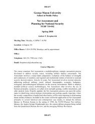
study corridor that was conducive to the agreed project timeline and deliverables. Figure 3-1 illustrates<br />
the base geographic region <strong>of</strong> the study corridor.<br />
13<br />
Figure 3-1: Study Base Map<br />
Defining the study corridor for purposes <strong>of</strong> preparing model forecasts, assessing regional demographic<br />
patterns, and evaluating a cost-benefit analysis, HSR operations and the service area are explained in<br />
the following definitions <strong>of</strong> HSR and conventional rail. Identifying the general types <strong>of</strong> HSR describes; the<br />
best function and design for the study corridor.<br />
• HSR – Express: Frequent, express service between major population centers 200–600 miles apart,<br />
with few intermediate stops. Top speeds <strong>of</strong> at least 150 mph on completely grade-separated,<br />
dedicated rights-<strong>of</strong>-way (with the possible exception <strong>of</strong> some shared track in terminal areas). It is<br />
intended to relieve air travel and highway capacity constraints.<br />
• HSR – Regional: Relatively frequent service between major and moderate population centers 100–<br />
500 miles apart, with some intermediate stops. Top speeds <strong>of</strong> 110–150 mph, grade-separated, with
<strong>Cost</strong> <strong>Benefit</strong> <strong>Analysis</strong> <strong>of</strong> <strong>Washington</strong>-<strong>Richmond</strong> <strong>High</strong>-<strong>Speed</strong> <strong>Rail</strong> Spring 2010<br />
14<br />
some dedicated and some shared track using positive train control technology. Intended to relieve<br />
highway and, to some extent, air travel capacity constraints.<br />
• Emerging HSR: Developing corridors <strong>of</strong> 100–500 miles, with strong potential for future HSR<br />
regional and/or express service. Top speeds <strong>of</strong> up to 90–110 mph on primarily shared track<br />
eventually using positive train control technology, with advanced grade crossing protection or<br />
separation. Intended to develop the passenger rail market, and provide some relief to other modes.<br />
• Conventional <strong>Rail</strong>: Traditional intercity passenger rail service <strong>of</strong> more than 100 miles with as few<br />
as one to as many as 7–12 daily frequencies; may or may not have strong potential for future HSR<br />
service. Top speeds <strong>of</strong> 79 mph to 90 mph generally on shared track. It is intended to provide travel<br />
options and to develop the passenger rail market.<br />
The above definitions evaluate HSR design potential based on population centers and achievable<br />
speeds.<br />
Today, the study corridor is described as a conventional and aged rail line that requires many<br />
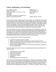
improvements to operate HSR passenger service. As shown in the 2009 population map, Figure 3-2, the<br />
study corridor contains city population concentrations within travel distances desired for HSR. The<br />
study corridor, is best described as an emerging HSR, especially since the corridor length is<br />
approximately 100 miles and design speeds are between 90 -110 mph.<br />
Figure 3-2: 2009 Population Map
<strong>Cost</strong> <strong>Benefit</strong> <strong>Analysis</strong> <strong>of</strong> <strong>Washington</strong>-<strong>Richmond</strong> <strong>High</strong>-<strong>Speed</strong> <strong>Rail</strong> Spring 2010<br />
15<br />
Figure 3-3: Population <strong>of</strong> Cities for Proposed Southeast <strong>High</strong>-<strong>Speed</strong> <strong>Rail</strong> Line<br />
3.2. Existing Operating Conditions<br />
The study corridor accommodates multiple train operators-Amtrak passenger rail service, CSX freight rail<br />
service, and Virginia <strong>Rail</strong>way Express (VRE) commuter rail service. All trains travel at a maximum average<br />
speed <strong>of</strong> 70 mph. The existing operations <strong>of</strong> each service provider are characterized below.<br />
CSX: CSX is a private company that provides service for multiple commodities including natural<br />
resources, general merchandise, and intermodal/auto units. CSX owns 25% <strong>of</strong> railway infrastructure in<br />
Virginia, including the track within the study corridor. According to the Virginia Department <strong>of</strong> <strong>Rail</strong> and<br />
Public Transportation (DRPT), CSX moves an annual total rail tonnage and rail through tonnage <strong>of</strong> nearly<br />
5-15 million commodity tons within the study corridor and it operates approximately 30 trains per day.<br />
VRE: VRE is a public passenger rail system that provides commuter rail service from Fredericksburg and<br />
Manassas, VA to <strong>Washington</strong>, D.C. Along the study corridor, the VRE Fredericksburg Line operates 15<br />
daily trains, northbound during morning peak hours (5:00 AM – 9:00 AM) and southbound during<br />
evening peak hours (3:00 PM – 8:30 PM), Monday through Friday. Service is available at 12 stations<br />
with headways <strong>of</strong> 20 – 30 minutes. In FY 2008 - FY 2009 VRE ridership was 3,857,646 passengers with<br />
approximately 2,122,000 (55%) using the Fredericksburg Line.<br />
Amtrak: Amtrak is privately run, federally owned, passenger rail service that provides regional and long<br />
distance service across the U.S. In FY 2008 – FY 2009 Amtrak ridership in Virginia was an estimated<br />
1,037,663 passengers with approximately 705,600 passengers (68%) traveling within the study corridor.<br />
Amtrak currently operates 8-10 daily trains (Monday – Friday), 4-5 regional trains and 5 long haul trains<br />
in the study corridor, which include:<br />
Regional Trains<br />
• Four daily northeast regional routes between Boston, MA and <strong>Richmond</strong>, VA and Newport<br />
News, VA;<br />
Long-Haul Trains<br />
• One daily Carolinian route between New York City and Charlotte, NC;<br />
• One daily Palmetto route between Savannah, GA and New York City;<br />
• One daily Silver Star route between Miami/Tampa, FL and New York City;
<strong>Cost</strong> <strong>Benefit</strong> <strong>Analysis</strong> <strong>of</strong> <strong>Washington</strong>-<strong>Richmond</strong> <strong>High</strong>-<strong>Speed</strong> <strong>Rail</strong> Spring 2010<br />
16<br />
• One daily Silver Meteor route between Miami FL and New York City;<br />
• One daily Auto Train route between Sanford, FL and Lorton, VA.<br />
Of the four daily northeast regional route trains, two operate within the peak morning period, one<br />
operates during the mid-day period, and one operates during the late evening. Northeast regional route<br />
trains account for approximately 50% <strong>of</strong> annual Virginia ridership, and other long haul trains account for<br />
nearly 40% <strong>of</strong> ridership within the study corridor. Other weekend service routes are available within the<br />
study corridor; however these routes are not listed or considered in the daily commuter analysis for this<br />
report.<br />
The study rail corridor is utilized by all three service operators. CSX is the sole owner, control operator,<br />
and dispatcher <strong>of</strong> the rail line; therefore, passenger rail service must operate as a complimentary service<br />
and not conflict or negatively impact freight rail movement. Common positions taken by the freight rail<br />
industry in response to accommodating passenger rail service are:<br />
• Freight railroads should be fully compensated for the use <strong>of</strong> their property by passenger trains;<br />
• Absent voluntary negotiated agreements, freight railroads should not be forced to give<br />
passenger rail operators access to their property;<br />
• Freight railroads should not be expected to subsidize passenger rail; and<br />
• Freight railroads do not want exposure to any liability associated with passenger rail service. At<br />
a minimum, freight railroads expect some enforceable limits on liability.<br />
One area with which operators have struggled is balancing on-time performance <strong>of</strong> all three services.<br />
Amtrak and VRE have reported drastic fluctuations in on-time performance related to internal<br />
operational problems, but also due to rail line congestion and CSX’s operation hierarchy. Passenger rail<br />
must frequently negotiate with freight rail owners to maintain acceptable performance levels as<br />
demand <strong>of</strong> both passenger and freight markets change.<br />
<strong>Rail</strong> capacity can be measured using many variables, such as topography, load factors, dwell times,<br />
operating speeds, train length, and track curvature. For the purpose <strong>of</strong> this report, a capacity<br />
measurement method was borrowed from the 2007 National <strong>Rail</strong> Freight Infrastructure Capacity and<br />
Investment Study, prepared by Cambridge Systematics, Inc. in order to determine capacity. The method<br />
calculates a volume-to-capacity ratio for archetypical railway corridors based on the number <strong>of</strong> tracks,<br />
number <strong>of</strong> daily trains, and operational control type. The following table shows the calculation <strong>of</strong><br />
existing rail capacity for the study corridor. The method is described in Appendix E.
<strong>Cost</strong> <strong>Benefit</strong> <strong>Analysis</strong> <strong>of</strong> <strong>Washington</strong>-<strong>Richmond</strong> <strong>High</strong>-<strong>Speed</strong> <strong>Rail</strong> Spring 2010<br />
17<br />
Table 3-1: Existing Capacity <strong>Analysis</strong> for Study <strong>Rail</strong> Corridor 12<br />
Service Provider # <strong>of</strong> Trains per Day<br />
CSX 25<br />
Amtrak 18<br />
VRE 15<br />
Total 58<br />
# <strong>of</strong><br />
Tracks<br />
Control<br />
Type<br />
Max<br />
Capacity<br />
LOS<br />
Grade V/C Ratio<br />
2 CTC 75 D 0.77<br />
Based on service timetables and DRPT reports, CSX, VRE, and Amtrak operate approximately 54 daily<br />
trains along the study corridor. The study corridor has a practical maximum capacity <strong>of</strong> 75 trains per<br />
day. The existing V/C ratio <strong>of</strong> the study corridor is calculated dividing current train capacity by maximum<br />
train capacity. For the D.C. to <strong>Richmond</strong> corridor it is 0.72 (54/75), operating at a level <strong>of</strong> service (LOS)<br />
D. This indicates that the rail corridor is moderately congested and operates near full capacity.<br />
3.3 Commuting Conditions 13<br />
Origin and Destination<br />
The origin and destination analysis focuses on workers in three areas <strong>of</strong> residential origin – Northern<br />
Virginia/D.C., the middle region, and the <strong>Richmond</strong> area – and three mode categories by which these<br />
residents commute – all modes, single occupant vehicle (SOV), and rail. This analysis reveals potential<br />
commuters likely to convert to using HSR, should it become available.<br />
Northern Virginia and D.C. Region 14<br />
This area by far has the most commuters, the majority <strong>of</strong> which remain in the D.C. Metro area for work.<br />
Of the more than 1.6 million workers, 67 % drive alone while those using commuter rail and Amtrak are<br />
only slightly more than a quarter percent. Commuters in this region are not likely to benefit from HSR in<br />
the study corridor because they do not travel distances long enough to warrant its usage. The number <strong>of</strong><br />
workers commuting by SOV is substantially less than those in the <strong>Richmond</strong> and middle-regions areas,<br />
likely due to the existence <strong>of</strong> more travel options.<br />
Middle Region (Stafford, Spotsylvania, Fredericksburg, Caroline, and King George)<br />
Fredericksburg and the surrounding counties have approximately 120,000 commuters. While many <strong>of</strong><br />
them remain in the middle region for work, numerous commute to Northern VA and D.C. Of all three<br />
regions, this area represents the greatest number <strong>of</strong> residents that commute by rail, at 1.3%., likely due<br />
12<br />
Does not include three year pilot program funded by the Commonwealth <strong>of</strong> Virginia to operate two new Amtrak<br />
trips between <strong>Richmond</strong> and <strong>Washington</strong>, D.C. that will begin mid-July 2010.<br />
13<br />
Data used for current commuting conditions was obtained from the Census Transportation Planning Package<br />
(CTPP) 2000<br />
14<br />
See Appendix E for maps <strong>of</strong> Northern Virginia and DC Region; Middle Region; and, <strong>Richmond</strong> Region
<strong>Cost</strong> <strong>Benefit</strong> <strong>Analysis</strong> <strong>of</strong> <strong>Washington</strong>-<strong>Richmond</strong> <strong>High</strong>-<strong>Speed</strong> <strong>Rail</strong> Spring 2010<br />
to the fact that VRE is a viable option for those desiring time savings compared to commuting alone by<br />
personal auto. Current rail users would likely be a captive audience for HSR because they are already<br />
comfortable using this mode and would recognize the benefit <strong>of</strong> additional time savings. SOV data<br />
reveals that 76% <strong>of</strong> middle region residents drive alone, the majority <strong>of</strong> whom travel north, making<br />
them a primary target for HSR.<br />
18<br />
<strong>Richmond</strong> Region (<strong>Richmond</strong>, Chesterfield, Hanover, Henrico)<br />
Most <strong>Richmond</strong> area residents work in the surrounding area; however, some commute to the D.C.<br />
metro area. The majority <strong>of</strong> commuters traveling further north commute alone by car, as transportation<br />
options are limited. Two Amtrak trains run northbound in the morning from this region, which is most<br />
likely being used by approximately 25 residents, or 0.01%, who indicated they travel by rail to the D.C.<br />
area. Of the 86% <strong>of</strong> SOV commuters, those traveling to the D.C. area would be potential converts to<br />
HSR.<br />
Persons working in Metro D.C. who prefer to live further south are most likely to reside in the middle<br />
region, as opposed to the <strong>Richmond</strong> region when considering housing prices and commuting distance.<br />
Residents already living in the <strong>Richmond</strong> region would benefit from HSR because it would make areas<br />
north <strong>of</strong> <strong>Richmond</strong> more feasible in terms <strong>of</strong> employment opportunities.<br />
Existing Congestion<br />
Figure 3-4: Existing Corridor Congestion<br />
Level <strong>of</strong> Service (LOS) is the term used among state<br />
highway administrations to show how much is on a<br />
particular freeway or multilane highway. The different<br />
levels <strong>of</strong> service are separated into grades A through F<br />
and each level depicted with different colors.<br />
Level A – Free flow conditions; green color, not depicted<br />
on this map<br />
Level B – Allows for free flow speeds, but not all the time,<br />
acceptable to drive in by most standards; darkest green.<br />
Level C – Slightly below free flow speeds, start to notice<br />
decline in maneuverability. Lighter green.<br />
Level D – Slightly near capacity, not much freedom to<br />
maneuver, congestion in noticeable; yellow color<br />
Level E – At capacity, any small disruption will severely<br />
slow down traffic; orange color<br />
Level F – Congested, with a breakdown in flow. Not<br />
gridlock, but slowly moving; red color.<br />
U.S. Interstate 95 and U.S. Route 1 serve as the major thoroughfares for auto trips approximately 107<br />
miles in distance. The majority <strong>of</strong> the I-95 corridor between <strong>Washington</strong>, D.C. and <strong>Richmond</strong> has an LOS<br />
<strong>of</strong> F, indicating heavy congestion and slow moving speeds during peak period travel. A significant stretch<br />
<strong>of</strong> the corridor operates at the slightly improved LOS <strong>of</strong> D in Caroline County, between Hanover and
<strong>Cost</strong> <strong>Benefit</strong> <strong>Analysis</strong> <strong>of</strong> <strong>Washington</strong>-<strong>Richmond</strong> <strong>High</strong>-<strong>Speed</strong> <strong>Rail</strong> Spring 2010<br />
Spotsylvania counties. Hanover County is the only jurisdiction with stretches <strong>of</strong> LOS C, operating at the<br />
best level <strong>of</strong> service along the corridor, although still slightly below free flow speeds. Heading north<br />
from Spotsylvania County commuters experience congestion until south <strong>of</strong> Alexandria City, where there<br />
are short stretches <strong>of</strong> LOS E and then LOS D.<br />
Congestion is costly. The Texas Transportation Institute estimates that congestion costs area residents<br />
$2.73 billion, or the equivalent <strong>of</strong> a new Woodrow Wilson Bridge each year. A breakdown <strong>of</strong> annual<br />
costs attributed to congestion include:<br />
19<br />
• $2.73 billion congestion cost for the region<br />
• 240 million gallons <strong>of</strong> fuel wasted<br />
• 160 million hours wasted sitting in traffic<br />
• $925 cost per driver<br />
• $780 cost per person<br />
• 76 hours <strong>of</strong> delay per driver 15<br />
Departure time<br />
Home departure time represents the time that workers leave their homes in the morning to travel to<br />
work. The data includes times that workers leave their homes based on 30-minute increments between<br />
5 a.m. and 9 a.m. This information was analyzed to give Amtrak an idea <strong>of</strong> how to most efficiently<br />
schedule trains to meet the demands <strong>of</strong> commuters. When used in conjunction with the origindestination<br />
and travel time data, it becomes apparent that departure time depends on where a<br />
commuter is traveling for work and the length <strong>of</strong> time it takes to get there.<br />
The majority <strong>of</strong> commuters in Northern Virginia and D.C. leave their homes between 7:00 and 8:29 a.m.<br />
In Manassas, Prince William, and Stafford counties; however, there is a greater number <strong>of</strong> commuters<br />
that depart between 6:00 and 6:29 a.m. Considering these commuters live further from large<br />
employment centers, such as D.C. and Fairfax County, it is not surprising that they may be commuting<br />
longer distances and using various modes <strong>of</strong> travel which require more time.<br />
The <strong>Richmond</strong> region demonstrates a similar pattern <strong>of</strong> commuters departing between 7:00 and 8:29<br />
a.m. Compared to neighboring counties, Chesterfield County shows a greater number <strong>of</strong> workers leaving<br />
home before 7:29 a.m., which similar to outlying jurisdictions in Northern Virginia, could be due to<br />
distance traveling and/or the use <strong>of</strong> multiple modes to get to work.<br />
In all counties and the District there is a significant decrease in the number <strong>of</strong> commuters departing<br />
during the 8:30 – 8:59 a.m. period, indicating the probability that most workers begin working before<br />
9:00 a.m.<br />
15 Transportation Need for the Future <strong>of</strong> the National Capital Region (The Greater <strong>Washington</strong> Board <strong>of</strong> Trade).
<strong>Cost</strong> <strong>Benefit</strong> <strong>Analysis</strong> <strong>of</strong> <strong>Washington</strong>-<strong>Richmond</strong> <strong>High</strong>-<strong>Speed</strong> <strong>Rail</strong> Spring 2010<br />
20<br />
Travel Time<br />
The District <strong>of</strong> Columbia and counties along the study corridor display a greater number <strong>of</strong> workers<br />
commuting 45 minutes or longer than jurisdictions located further from the corridor.<br />
Jurisdictions with the highest number <strong>of</strong> commuters traveling 45 minutes or longer are primarily in<br />
Northern VA, including D.C., and south to Spotsylvania County, capturing 6,036-121,835 workers. From<br />
greatest to least, these jurisdictions in the service area include Fairfax and Prince William counties, the<br />
District <strong>of</strong> Columbia, Loudoun, Stafford, and Arlington counties, Alexandria City, Spotsylvania,<br />
Chesterfield, Fauquier, and Henrico counties, and <strong>Richmond</strong> City.<br />
The middle category <strong>of</strong> jurisdictions captures from 1,566-6,035 commuters traveling 45 minutes or<br />
longer to work. Other than five <strong>of</strong> the jurisdictions located more closely to the study corridor, they<br />
mostly extend further west and east <strong>of</strong> the corridor. Jurisdictions in this range include, from greatest to<br />
least, Manassas, Culpeper, Hanover, Louisa, Powhatan, Caroline, and Orange counties, Fairfax City,<br />
Westmoreland County, Manassas Park City, and Goochland, King George, Prince George, and<br />
Fredericksburg counties.<br />
The least number <strong>of</strong> commuters traveling 45 minutes or more reside mainly in jurisdictions that are<br />
located furthest east and south <strong>of</strong> the corridor study area, with the exception <strong>of</strong> the City <strong>of</strong> Falls Church<br />
in Northern Virginia.<br />
While the aforementioned analysis includes commuters using all modes, a closer look at travel time by<br />
individual mode reveals that commuters driving alone for 45 minutes or greater follows a similar pattern<br />
to that <strong>of</strong> all modes. <strong>Rail</strong> commuters however, demonstrate a major shift in pattern. Jurisdictions south<br />
<strong>of</strong> Spotsylvania County reflect a negligible number <strong>of</strong> commuters traveling by rail for 45 minutes or<br />
longer. In jurisdictions north <strong>of</strong> Spotsylvania a much greater number <strong>of</strong> commuters are using rail and<br />
traveling for 45 minutes or longer.<br />
Travel <strong>Cost</strong><br />
The existing rail market demand within the study corridor is represented by evaluating the cost<br />
difference <strong>of</strong> operating an automobile compared to riding Amtrak. Figure 3-5 shows the counties within<br />
the service area where the cost to ride Amtrak is at least 1% less than driving. For example, commuters<br />
traveling from Henrico County, VA to <strong>Washington</strong>, D.C. have a potential cost savings <strong>of</strong> 10% - 19% when<br />
riding Amtrak instead <strong>of</strong> driving. The gray regions <strong>of</strong> the map identify the counties where commuters<br />
are not likely to save money by riding Amtrak. Figure 3-6 shows the counties where the cost to ride<br />
Amtrak is at least 1% less than driving to <strong>Richmond</strong>, VA.<br />
The average automobile commute calculated for the cost maps is $0.45 per mile, which includes the<br />
costs <strong>of</strong> gasoline, wear and tear per 15,000 annual miles traveled, average insurance, and purchase/loan<br />
payment. The cost <strong>of</strong> using Amtrak rail was calculated based on the average ticket price for traveled<br />
distance. <strong>Cost</strong> effective regions within the service area could expand with the implementation <strong>of</strong> HSR<br />
operations, particularly along the corridor.
<strong>Cost</strong> <strong>Benefit</strong> <strong>Analysis</strong> <strong>of</strong> <strong>Washington</strong>-<strong>Richmond</strong> <strong>High</strong>-<strong>Speed</strong> <strong>Rail</strong> Spring 2010<br />
21<br />
Figure 3-5: Commuter <strong>Cost</strong> Map<br />
Figure 3-6: <strong>Richmond</strong> Commuter <strong>Cost</strong> Map<br />
Understanding current travel behavior and commuting patterns is essential for identifying potential<br />
customers for the HSR line between <strong>Richmond</strong> and <strong>Washington</strong> D.C.<br />
According to the data, the greatest potential for Amtrak to attract customers to the HSR service lies in<br />
the ability to attract SOV commuters residing in the Fredericksburg and <strong>Richmond</strong> areas who travel to<br />
Northern VA and D.C. Considering congestion on I-95, travel times <strong>of</strong> 45 minutes and greater, and the<br />
early times at which commuters leave their homes, these travelers are likely looking for options.<br />
Commuters have various reasons for choosing their travel mode. Amtrak high-speed trains, <strong>of</strong>fered<br />
affordably and at times convenient for commuters, would provide a reduction in overall commute time<br />
and relief from traffic congestion.
<strong>Cost</strong> <strong>Benefit</strong> <strong>Analysis</strong> <strong>of</strong> <strong>Washington</strong>-<strong>Richmond</strong> <strong>High</strong>-<strong>Speed</strong> <strong>Rail</strong> Spring 2010<br />
3.4 Environmental Conditions<br />
22<br />
Figure 3-7: On Road Emissions<br />
The National Emissions Inventory (NEI) is developed<br />
every three years by EPA. The NEI is a national<br />
emissions inventory that includes both stationary<br />
and mobile sources that emit hazardous air<br />
pollutants (HAPs). Section 112(b) <strong>of</strong> the Clean Air Act<br />
identifies 188 pollutants as HAPs, which are<br />
generally defined as pollutants that are known or<br />
suspected to cause serious health problems. The NEI<br />
contains emission estimates for major sources,<br />
nonpoint sources, mobile sources, and other sources<br />
which do not fall into these categories.<br />
Onroad mobile sources include “licensed motor<br />
vehicles, including automobiles, trucks, buses, and<br />
motorcycles.”<br />
The orange and red shading on the onroad emissions map indicates levels that are higher than 691,028<br />
pounds <strong>of</strong> emissions per year. Counties and cities in the corridor service area that fall into the high<br />
emissions category, ranging from highest to lowest are Fairfax, Loudoun, and Prince William counties,<br />
<strong>Washington</strong> D.C., and Chesterfield, Hanover, and Henrico counties.<br />
The middle categories are defined as counties and cities that have moderate levels <strong>of</strong> onroad emissions,<br />
ranging from 127,104 to 691,027. Jurisdictions located in the service area and included in this range<br />
from highest to lowest are <strong>Richmond</strong> City, Arlington and Stafford counties, Alexandria City, Spotsylvania,<br />
Fauquier, Westmoreland, Louisa, New Kent counties, Charles City, Essex, Goochland, Culpeper, and King<br />
and Queen counties, and Fairfax City.<br />
The jurisdictions showing the lowest amount <strong>of</strong> onroad emissions located in the corridor study area are<br />
Caroline, King William, Powhatan, and King George counties, Falls Church, Manassas, Manassas Park,<br />
Fredericksburg, and Colonial Heights cities. These areas have onroad emissions that fall into the range <strong>of</strong><br />
zero to 127,103 pounds per year.<br />
Looking more closely at the data, onroad emissions as a percent <strong>of</strong> total emissions tells a different story.<br />
While Charles City falls into the moderate category for total onroad emissions, onroad emissions makes<br />
up 58% <strong>of</strong> the county’s total emissions. The counties <strong>of</strong> Middlesex, Westmoreland, Kind and Queen, and<br />
Loudoun range from 45% - 48% onroad emissions as a percent <strong>of</strong> the total. For jurisdictions that show<br />
more than half or nearly half <strong>of</strong> their onroad emissions as making up total emissions, this could indicate<br />
they simply have less nonpoint emissions sources and should not be used as a gauge in obtaining<br />
emissions reductions until it is fully understood.
<strong>Cost</strong> <strong>Benefit</strong> <strong>Analysis</strong> <strong>of</strong> <strong>Washington</strong>-<strong>Richmond</strong> <strong>High</strong>-<strong>Speed</strong> <strong>Rail</strong> Spring 2010<br />
3.5 Future Considerations<br />
For purposes <strong>of</strong> this report, a third track is assumed to be completed within the study corridor, which<br />
would allow for a future practical maximum capacity <strong>of</strong> 133 trains per day. Increased operations <strong>of</strong> train<br />
operators is unknown, therefore it is assumed that train operation within the future study corridor could<br />
increase to approximately 79 trains per day to maintain an operating LOS <strong>of</strong> D or better.<br />
23
<strong>Cost</strong> <strong>Benefit</strong> <strong>Analysis</strong> <strong>of</strong> <strong>Washington</strong>-<strong>Richmond</strong> <strong>High</strong>-<strong>Speed</strong> <strong>Rail</strong> Spring 2010<br />
4. What is a <strong>Cost</strong>-<strong>Benefit</strong> <strong>Analysis</strong>?<br />
A cost-benefit analysis is a term that typically refers to:<br />
24<br />
• Helping to appraise, or assess, the case for a project or proposal; and<br />
• An informal approach to making economic decisions <strong>of</strong> any kind. 16<br />
In a transportation context, a cost-benefit analysis attempts to measure the dollar value <strong>of</strong> the benefits<br />
and the costs to all the members <strong>of</strong> society where “society” is all residents <strong>of</strong> the United States on a net<br />
present value basis. The benefits represent a dollar measure to the extent the lives <strong>of</strong> people are made<br />
better by a project. The benefits represent the amount that all the people in society would jointly be<br />
willing to pay to carry out the project, and feel as if they had generated enough benefits to justify the<br />
project’s costs, accounting for the relative timing <strong>of</strong> those benefits and costs. In some cases, benefits<br />
may be difficult to measure monetarily. Therefore, when preparing a cost-benefit analysis, it is helpful<br />
to describe the nature <strong>of</strong> each major benefit. <strong>Benefit</strong>s should be quantifiable (e.g., in number <strong>of</strong> users<br />
making use <strong>of</strong> a transportation facility). Lastly, benefits should be measured in dollar terms, or<br />
monetized. This allows the benefits to be directly compared to the monetary costs <strong>of</strong> the project.<br />
<strong>Benefit</strong>s and costs must be estimated for each year <strong>of</strong> the project after work has begun. These annual<br />
benefits and costs must be discounted to the present using an appropriate discount rate so that a<br />
present value <strong>of</strong> the benefits and a present value <strong>of</strong> the costs is appropriately calculated and compared.<br />
The following provides a simplified example <strong>of</strong> discounted costs and benefits from a road project that<br />
provides travel time savings to local travelers over the course <strong>of</strong> five years following a one-year period<br />
<strong>of</strong> construction.<br />
16 “Dictionary.com,” in , 2010.
<strong>Cost</strong> <strong>Benefit</strong> <strong>Analysis</strong> <strong>of</strong> <strong>Washington</strong>-<strong>Richmond</strong> <strong>High</strong>-<strong>Speed</strong> <strong>Rail</strong> Spring 2010<br />
Calendar<br />
Year<br />
25<br />
Project<br />
Year<br />
Affected<br />
Drivers<br />
Travel Time Saved<br />
(hours) 1<br />
Table 4-1: <strong>Cost</strong> <strong>Benefit</strong> Sample<br />
Total Value <strong>of</strong><br />
Time Saved<br />
($2008) 2<br />
Initial<br />
<strong>Cost</strong>s<br />
($2008)<br />
Operations &<br />
Maintenance <strong>Cost</strong>s<br />
($2008) 3<br />
Undiscounted Net<br />
<strong>Benefit</strong>s<br />
Additional information on cost-benefit analysis preparation can be found in the Office <strong>of</strong> Management<br />
and Budget (OMB) Circulars A-4 and A-94 in preparing their analysis<br />
(http://www.whitehouse.gov/omb/circulars). Circular A-4 also cites textbooks on cost-benefit analysis<br />
(e.g., Mishan and Quah). 17<br />
4.1 <strong>Cost</strong> <strong>Benefit</strong> <strong>Analysis</strong> vs. Economic Impact <strong>Analysis</strong><br />
It is important to recognize that a cost-benefit analysis is not an economic impact analysis. As previously<br />
stated, a cost-benefit analysis attempts to measure the dollar value <strong>of</strong> the benefits and the costs to all<br />
the members <strong>of</strong> society.<br />
Conversely, an economic impact analysis focuses on local benefits rather than national benefits. Some<br />
<strong>of</strong> the benefits that are counted in an economic impact analysis, such as diversion <strong>of</strong> economic activity<br />
from one region <strong>of</strong> the country to another, represent benefits to one part <strong>of</strong> the country but costs to<br />
another part, so they are not benefits from the standpoint <strong>of</strong> the nation as a whole.<br />
Moreover, economic impact analyses estimate impacts rather than benefits, and the impacts are<br />
normally much larger than the benefits. For example, the total payroll <strong>of</strong> workers on a project is usually<br />
considered one <strong>of</strong> the impacts in an economic impact analysis. The total payroll is not a measure <strong>of</strong> the<br />
benefits <strong>of</strong> the project for two reasons. First, a payroll is a cost to whoever pays the employees, at the<br />
same time that it is a benefit to the employees, so it is not a net benefit. Second, even for the<br />
employees, the employees have to work for their wages, so the amount they are paid is not a net<br />
benefit to them – it is a benefit only to the extent that they value their wages more than the cost to<br />
them <strong>of</strong> having to be at work every day.<br />
Economic impact analyses also consider real estate investments to be one <strong>of</strong> the economic impacts <strong>of</strong> a<br />
project. The full value <strong>of</strong> such an investment is not a benefit, however, because the benefit <strong>of</strong> the<br />
investments to the community in which they are made is balanced by the cost <strong>of</strong> the investment to the<br />
17 E.J. Mishan and Euston Quah, <strong>Cost</strong>-<strong>Benefit</strong> <strong>Analysis</strong>, 5th ed. (New York: Routeledge, 2007).<br />
Discounted at<br />
7%<br />
2011 1 $38,500,000 $6,000,000 -$44,500,000 -$41,588,785<br />
2012 2 80,000 1,040,000 $14,248,000 $700,000 $13,548,000 $11,833,348<br />
2013 3 95,000 1,235,000 $16,919,500 $700,000 $16,219,500 $13,239,943<br />
2014 4 100,000 1,300,000 $17,810,000 $700,000 $17,110,000 $13,053,137<br />
2015 5 102,000 1,326,000 $18,166,200 $700,000 $17,466,200 $12,453,159<br />
2016 6 109,000 1,417,000 $19,412,900 $700,000 $18,712,900 $12,469,195<br />
NPV $21,459,998<br />
1. Number <strong>of</strong> drivers times three minutes a day (3/60 hours) over 260 workdays<br />
2. Hours at $13.70 per hour ($2008)<br />
3. Includes costs from delays to users during construction
<strong>Cost</strong> <strong>Benefit</strong> <strong>Analysis</strong> <strong>of</strong> <strong>Washington</strong>-<strong>Richmond</strong> <strong>High</strong>-<strong>Speed</strong> <strong>Rail</strong> Spring 2010<br />
investor. Because these investments are a cost as well as a benefit, they are not a net benefit as in a<br />
cost-benefit analysis.<br />
There is <strong>of</strong>ten an element <strong>of</strong> benefit in these impacts. A worker who gets a higher paying job as a result<br />
<strong>of</strong> a transportation investment project benefits if he or she works just as hard as he or she did at his or<br />
her previous job but is paid more. Such projects produce benefits by increasing the productivity <strong>of</strong><br />
labor. A transportation investment project that increases the value and productivity <strong>of</strong> land and thus<br />
induces real estate investment can also provide a benefit, but the benefit must be measured net <strong>of</strong> the<br />
cost <strong>of</strong> making the real estate investment. Measuring these labor productivity effects requires a careful<br />
analysis <strong>of</strong> the local labor market and how that market is changed by the transportation investment.<br />
Similarly, measuring the effects <strong>of</strong> transportation projects on the productivity <strong>of</strong> land requires careful<br />
netting out <strong>of</strong> increases in land values that are compensated by costs <strong>of</strong> real estate investment and<br />
increases in land values that in effect capitalize other types <strong>of</strong> benefits that have already been counted,<br />
such as time savings.<br />
The benefits that should be reported for transportation projects include:<br />
26<br />
• Improved condition <strong>of</strong> existing transportation facilities and systems;<br />
• Long-term growth in employment, production, or other high-value economic activity;<br />
• Improved energy efficiency, reduced dependence on oil and reduced greenhouse gas emissions;<br />
• Reduced adverse impacts <strong>of</strong> transportation on the natural environment;<br />
• Reduced number, rate and consequences <strong>of</strong> surface transportation-related crashes, injuries and<br />
fatalities;<br />
• Any other benefits claimed in the project’s cost-benefit analysis.<br />
4.2 Affected Population<br />
Because these improvements are associated with improvements along a passenger rail line, the costbenefit<br />
analysis should clearly identify the population that the project will affect and measure the<br />
number <strong>of</strong> passengers affected by the project. Although the improvements being considered are<br />
directly related to passenger rail movements, the rail line being impacted has both passenger and<br />
freight movements that need to be addressed as part <strong>of</strong> the analysis. If possible, passenger and freight<br />
traffic should be measured in passenger-miles and freight ton-miles (and possibly value <strong>of</strong> freight).<br />
4.3 Discounting<br />
When preparing the cost-benefit analysis, the analysis should discount future benefits and costs to<br />
present values using a real discount rate <strong>of</strong> seven percent, following guidance provided by the Office <strong>of</strong><br />
Management and Budget (OMB) in Circulars A–4 and A–94 1819 .<br />
18 Circular A-4 (<strong>Washington</strong>, DC: Office <strong>of</strong> Management and Budget, September 17, 2003).<br />
19 Guidelines and Discount Rates for <strong>Benefit</strong>-<strong>Cost</strong> <strong>Analysis</strong> <strong>of</strong> Federal Programs (<strong>Washington</strong>, DC: Office <strong>of</strong><br />
Management and Budget).
<strong>Cost</strong> <strong>Benefit</strong> <strong>Analysis</strong> <strong>of</strong> <strong>Washington</strong>-<strong>Richmond</strong> <strong>High</strong>-<strong>Speed</strong> <strong>Rail</strong> Spring 2010<br />
In addition to the 7 percent discount rate, a 3 percent discount rate may be considered as part <strong>of</strong> the<br />
alternative analysis. A 3 percent discount rate should be used when alternative funds that are dedicated<br />
to the project would be other public expenditures and not private investment.<br />
The first step, the analysis should present the year-by-year stream <strong>of</strong> benefits and costs from the<br />
project. The analysis should clearly identify when the expected costs and benefits will occur. The<br />
beginning point for the year-by-year stream <strong>of</strong> benefits should be the first year in which the project will<br />
start generating costs or benefits. The ending point should be far enough in the future to encompass all<br />
<strong>of</strong> the significant costs and benefits resulting from the project but not to exceed the usable life <strong>of</strong> the<br />
asset without capital improvement. 20 In presenting these year-by-year streams, the analysis should<br />
measure them in constant or real dollars prior to discounting. The analysis should not add in the effects<br />
<strong>of</strong> inflation to the estimates <strong>of</strong> future benefits and costs prior to discounting. Once a yearly stream <strong>of</strong><br />
costs and benefits in constant dollars are generated, the analysis should discount these estimates to<br />
arrive at a present value <strong>of</strong> costs and benefits. The standard formula for the discount factor in any given<br />
year is 1/ (1 + r) t , where “r” is the discount rate and “t” measures the number <strong>of</strong> years in the future that<br />
the costs or benefits will occur. Infrequently, benefits or costs will be the same in constant dollars for all<br />
years. In these limited cases, the analysis can calculate the formula for the present value <strong>of</strong> an ordinary<br />
annuity instead <strong>of</strong> showing a year-by-year calculation. 21<br />
4.4 Baselines and Alternatives<br />
The baseline should be an assessment <strong>of</strong> the way the world would look if the proposed improvements<br />
were not implemented. Usually, it is reasonable to forecast that that baseline would resemble the<br />
present state. However, it is important to factor in any projected changes (e.g., economic growth,<br />
increased traffic volumes, or completion <strong>of</strong> already planned and funded projects) that would occur even<br />
if the proposed project were not carried forward. The benefits and costs in this case should thus be<br />
20 In some cases the analysis may use a fixed number <strong>of</strong> years to analyze benefits and costs (e.g., 20 years), even if<br />
the project will last longer than that and continue to have benefits and costs in later years. In these cases, the<br />
project will retain a “residual value” at the end <strong>of</strong> the analysis period. For instance, a new bridge may be expected<br />
to have a 100-year life, but the analysis period for the cost-benefit analysis might cover only 40 years. In such<br />
cases, a residual value can be claimed as a benefit (or cost <strong>of</strong>fset) for the asset at the end <strong>of</strong> the analysis period.<br />
One method to estimate the residual value is to calculate the percentage <strong>of</strong> the project that will not be<br />
depreciated or used up at the end <strong>of</strong> the analysis period and to multiply this percentage by the original cost <strong>of</strong> the<br />
project. Different components <strong>of</strong> the project may have different depreciation rates – land typically does not<br />
depreciate. The estimated residual value is assigned to the end <strong>of</strong> the analysis period and should then be<br />
discounted to its present value as would any other cost or benefit occurring at that time. Note that a residual<br />
value <strong>of</strong> a project can only be claimed if the project will be kept in operation beyond the end <strong>of</strong> the analysis period.<br />
If the project will be retired at that time, a salvage value (reflecting revenues raised from the decommissioning <strong>of</strong><br />
the project) can be claimed.<br />
21 See “The Present Value and Future Value <strong>of</strong> an Annuity Formula,” Bright Hub,<br />
http://www.brighthub.com/money/personal-finance/articles/17948.aspx For example, 10.594 is the discount<br />
factor that would be multiplied by an annual benefit to get the present value <strong>of</strong> a constant benefit stream over 20<br />
years at a discount rate <strong>of</strong> seven percent. If the constant annual benefit is $500,000, then the present value <strong>of</strong> the<br />
benefits is $5.297 million. In these limited cases, the analysis must show the calculation <strong>of</strong> the discount factor <strong>of</strong><br />
the ordinary annuity formula.<br />
27
<strong>Cost</strong> <strong>Benefit</strong> <strong>Analysis</strong> <strong>of</strong> <strong>Washington</strong>-<strong>Richmond</strong> <strong>High</strong>-<strong>Speed</strong> <strong>Rail</strong> Spring 2010<br />
limited to the marginal benefits (and marginal costs) <strong>of</strong> having the project completed in a shorter period<br />
<strong>of</strong> time and including the cost <strong>of</strong> expending resources on the project sooner than otherwise planned.<br />
In preparing a cost-benefit analysis, all costs and benefits <strong>of</strong> the project should be evaluated, including<br />
benefits and costs that fall outside <strong>of</strong> the immediate area where the project lies. Assuming a baseline<br />
scenario in which the owner <strong>of</strong> the facility performs no maintenance and ignores traffic problems is not<br />
realistic and will lead to the overstatement <strong>of</strong> project benefits.<br />
28
<strong>Cost</strong> <strong>Benefit</strong> <strong>Analysis</strong> <strong>of</strong> <strong>Washington</strong>-<strong>Richmond</strong> <strong>High</strong>-<strong>Speed</strong> <strong>Rail</strong> Spring 2010<br />
5. Project <strong>Cost</strong>s<br />
According to Rohit Aggarwala, a member <strong>of</strong> the New York State Assembly <strong>High</strong>-<strong>Speed</strong> <strong>Rail</strong> Task Force,<br />
historically major investments in surface transportation infrastructure have originated from dedicated<br />
state funding mechanisms as key drivers. 22 The federal government has historically taken a “wait-andsee”<br />
approach to allow states the freedom to develop their own initiatives. Following this, the federal<br />
government usually steps in to help organize the various state initiatives into a national network by<br />
standardizing successful processes identified by the initial work conducted by the states.<br />
In the current case <strong>of</strong> HSR development, the federal approach has been augmented by the availability <strong>of</strong><br />
ARRA funding to allow states with particularly strong rail initiatives a chance to obtain federal support.<br />
These projects must meet federal standards, which typically lead to a decrease in the build- time 23 .<br />
Currently, there are no dedicated sources <strong>of</strong> federal funding for HSR. As such, the onus remains on<br />
states to fully develop the scopes <strong>of</strong> their rail investment projects for HSR infrastructure and to establish<br />
dedicated sources <strong>of</strong> funding to ensure their viability.<br />
In “The States, New Modes, and Federal Transportation Policy: Lessons from History for <strong>High</strong>-<strong>Speed</strong><br />
<strong>Rail</strong>,” Dr. Aggarwala suggests that in the first decade <strong>of</strong> the 21 st century we will have entered a period<br />
where federal funding has been denied, and states will independently pursue a pattern <strong>of</strong> development<br />
with increasing public support for the successes <strong>of</strong> these independent projects. Historical development<br />
patterns follow the following five steps:<br />
29<br />
• Failed private attempts;<br />
• Mollification <strong>of</strong> failed federal bid for dedicated funding with a single unrepeated investment;<br />
• Independent state action;<br />
• Imitation by other states; and<br />
• Adoption <strong>of</strong> a dedicated federal funding mechanism and national transportation policy. 24<br />
In the Commonwealth <strong>of</strong> Virginia two sources <strong>of</strong> dedicated funding exist, which total $37.5 million<br />
annually 25 . The current HSR project designated in the 2009 State Resource Allocation Plan to receive the<br />
majority <strong>of</strong> support from these sources is the D.C. to <strong>Richmond</strong> Third Track Project. This project entails<br />
the construction <strong>of</strong> approximately 93 miles <strong>of</strong> track, bridges, stations, signals and curve realignments to<br />
22<br />
Aggarwala Rohit T. , “The States, New Modes, and Federal Transportation Policy: Lessons from History for <strong>High</strong>-<br />
<strong>Speed</strong> <strong>Rail</strong>.,” Transportation Quarterly 52, no. 3 (Summer 1998): 54.<br />
23<br />
Virginia Department <strong>of</strong> <strong>Rail</strong> and Public Transportation, “Virginia Department <strong>of</strong> <strong>Rail</strong> and Public Transit, Statewide<br />
<strong>Rail</strong> Plan Technical Update,” December 2009, 11-8, http://www.drpt.virginia.gov/studies/files/Chapter%2011%20-<br />
%20Projects.pdf.<br />
24<br />
Rohit T. , “The States, New Modes, and Federal Transportation Policy: Lessons from History for <strong>High</strong>-<strong>Speed</strong> <strong>Rail</strong>.,”<br />
54.<br />
25<br />
Virginia Department <strong>of</strong> <strong>Rail</strong> and Public Transportation, “Virginia Department <strong>of</strong> <strong>Rail</strong> and Public Transit, Statewide<br />
<strong>Rail</strong> Plan Technical Update,” 8-8.
<strong>Cost</strong> <strong>Benefit</strong> <strong>Analysis</strong> <strong>of</strong> <strong>Washington</strong>-<strong>Richmond</strong> <strong>High</strong>-<strong>Speed</strong> <strong>Rail</strong> Spring 2010<br />
accommodate maximum speeds <strong>of</strong> 90 mph, which is 20 mph over the current maximum operating<br />
speed.<br />
Virginia is now entering into step three <strong>of</strong> the HSR Third Track project after having been awarded some<br />
federal support. Funding for the $1.4 billion dollar project has been limited to less than 1% <strong>of</strong> these<br />
costs. As such this report assumes that federal funding will play a limited role as part <strong>of</strong> a public-private<br />
consortium dedicated to completing this HSR project. The limited federal support will also lead to an<br />
extended build-out period <strong>of</strong> 17 years which is beyond the seven-year period estimated in Phase I <strong>of</strong> the<br />
2009 DPRT Statewide Technical Report with full federal support. The following estimates for build-out<br />
times, construction costs, and debt service fees thus utilize this historic development pattern in<br />
transportation networks and assume limited federal support for the period to follow.<br />
5.1 Background<br />
The estimate <strong>of</strong> costs must pertain to the same project as the estimate <strong>of</strong> benefits. The analysis <strong>of</strong> costs<br />
should be equally as rigorous as the analysis <strong>of</strong> benefits. The lack <strong>of</strong> a useful analysis <strong>of</strong> expected project<br />
costs may be a basis for questioning the accuracy <strong>of</strong> the overall analysis. Additional information that<br />
should be included is operating, maintenance, and other life-cycle costs <strong>of</strong> the project, along with capital<br />
costs. In addition to construction costs, other direct costs may include design and land acquisition.<br />
External costs, such as noise, increased congestion, and environmental pollutants resulting from the use<br />
<strong>of</strong> the facility or related changes in usage on other facilities in the same network, should be considered<br />
as costs in the analysis. Additionally, it is appropriate to include costs to users during construction, such<br />
as delays and increased vehicle operating costs. The analysis should discount annual costs to arrive at a<br />
present value <strong>of</strong> the project’s cost.<br />
5.2 Infrastructure <strong>Cost</strong><br />
For rail infrastructure construction, unit cost categories were used based on the Virginia DRPT 2006 3 rd<br />
Track Feasibility Study. Unit costs consider many items within a unit price. An example would be the<br />
category-track work which includes ballast, ties, fasteners, other track materials, rail material, labor, and<br />
equipment needed to complete the work. 26 <strong>Cost</strong>s include the following categories:<br />
30<br />
• Track work<br />
• Special track work<br />
• Bridges<br />
• Drainage<br />
• Grade crossings<br />
• Utility relocation (underground piping)<br />
• Communications and signaling<br />
• Right-<strong>of</strong>-way<br />
• Stations and Buildings<br />
26 Virginia Department <strong>of</strong> <strong>Rail</strong> and Public Transportation, “Arkendale to Powell’s Creek Third Track Project:<br />
Financial Plan.,” 7.
<strong>Cost</strong> <strong>Benefit</strong> <strong>Analysis</strong> <strong>of</strong> <strong>Washington</strong>-<strong>Richmond</strong> <strong>High</strong>-<strong>Speed</strong> <strong>Rail</strong> Spring 2010<br />
31<br />
• Earthwork<br />
• Environmental and Permitting<br />
• Engineering services<br />
• Construction contingency<br />
• Annual debt service<br />
Due to the release <strong>of</strong> the 2 nd TIER II Environmental Impact Statement (EIS) report in late spring <strong>of</strong> 2010<br />
and pending priority schedules and engineering reports, several cost components have been relegated<br />
to be captured by a construction contingency equal to 30% <strong>of</strong> the construction costs. 27 These costs have<br />
been indexed with the 2012 dollar values and 7.5% annual debt service cost should the current costs<br />
need to be adjusted. 28 If it turns out that these additional costs do not materialize, the 30% contingency<br />
fee may be reduced based on the current construction timeline as needed.<br />
This report nears the two-year period when the preliminary engineering report for a total-build scenario<br />
would need to be undertaken and completed to prioritize the build schedule based on available funding.<br />
Since there has been a green light for construction <strong>of</strong> the Ark-Powell project in 2010, this would shave<br />
<strong>of</strong>f 11.4 miles <strong>of</strong> the 93 mile project and the project could be considered already underway, but to be<br />
safe, total project build time starting as <strong>of</strong> 2012 with 2012 dollar values is assumed to accommodate the<br />
estimated reporting time line to complete the preliminary engineering report.<br />
The total estimated cost <strong>of</strong> construction to complete the third track line between D.C. and<br />
<strong>Richmond</strong> comes to $1.63 billion dollars in 2012 dollar values, which accounts for the<br />
contingency construction fee and annual debt service costs over a 17-year period.<br />
27<br />
Virginia Department <strong>of</strong> <strong>Rail</strong> and Public Transportation, “<strong>Washington</strong>, D.C. to <strong>Richmond</strong> Third Track Feasibility<br />
Study,” 4-19.<br />
28<br />
David Levinson et al., “The Full <strong>Cost</strong> <strong>of</strong> <strong>High</strong>-<strong>Speed</strong> <strong>Rail</strong> : An Engineering Approach.,” The Annals <strong>of</strong> Regional<br />
Science (December 1996): 194, http://www.springerlink.com/content/brmxbug16762q5uc/fulltext.pdf.
<strong>Cost</strong> <strong>Benefit</strong> <strong>Analysis</strong> <strong>of</strong> <strong>Washington</strong>-<strong>Richmond</strong> <strong>High</strong>-<strong>Speed</strong> <strong>Rail</strong> Spring 2010<br />
5.3 Operating <strong>Cost</strong>s 29<br />
32<br />
Figure 5-1: Total Estimated Construction <strong>Cost</strong>s<br />
The operating costs for HSR systems, according to The Full <strong>Cost</strong> <strong>of</strong> <strong>High</strong>-speed <strong>Rail</strong>: an Engineering<br />
Approach 30 by Levinson, et al, can be categorized as follows:<br />
• Sales and administration costs - labor and automated machinery costs for providing tickets and<br />
information;<br />
• Shunting cost;<br />
• Train operations costs - labor costs required to service, drive and operate the trains;<br />
• Fuel or energy costs;<br />
• Maintenance <strong>of</strong> way; and<br />
• Maintenance <strong>of</strong> equipment.<br />
These are costs that Amtrak would incur to provide additional service as a part <strong>of</strong> this project.<br />
Considering the proposed technology <strong>of</strong> the SEHSR system, the most useful method to calculate<br />
increased operating and/or maintenance costs was to use the aggregated operating costs that Amtrak<br />
releases in their annual and monthly reports. Although possible to use the methods used in previous<br />
29 The Travel Demand Model used to determine these operating cost figures will be described in a following<br />
chapter<br />
30 Ibid., 203.
<strong>Cost</strong> <strong>Benefit</strong> <strong>Analysis</strong> <strong>of</strong> <strong>Washington</strong>-<strong>Richmond</strong> <strong>High</strong>-<strong>Speed</strong> <strong>Rail</strong> Spring 2010<br />
studies, using Amtrak’s numbers would be the most accurate. The proposed locomotives for the system<br />
are modern diesel locomotives that can operate at the intended 110 mph Maximum Authorized <strong>Speed</strong><br />
(MAS). These locomotives would not have substantially different operating costs than those currently in<br />
the Amtrak fleet. Given the similarities between current Amtrak operations and the proposed new trips,<br />
this is the most accurate estimate <strong>of</strong> operating costs for the new service.<br />
33<br />
Unit Unit <strong>Cost</strong><br />
Seat Mile 31 $0.237<br />
Train Mile 32 $69.980<br />
Passenger Mile 33 $0.554<br />
Table 5-1: Units and Unit <strong>Cost</strong>s for Amtrak Operating <strong>Cost</strong>s<br />
The operating costs can be calculated using both passenger miles traveled and train miles traveled as<br />
shown in Table 5-1. The cost per seat mile is equivalent to the cost per train mile because, for the<br />
purposes <strong>of</strong> this study, each train has a constant number <strong>of</strong> seats. Other studies assume each train has<br />
350 passenger seats. 34 Based on the above figures for seat mile and train mile costs, the average Amtrak<br />
train has 295 seats. This corridor is expected to have a higher volume than average, making 350<br />
passenger seats per train a reasonable estimate. To calculate the costs based on passenger mile, the<br />
results from the ridership model were used. The difference in ridership from the build and no-build<br />
scenarios was multiplied by the miles <strong>of</strong> travel and by the operating cost per passenger mile. In order to<br />
calculate the increased operating costs based on train mile, it was assumed that new trains would be<br />
added according to the phases proposed in the DRPT technical report. 35 The exact years the trains<br />
would start running was not indicated in the report, but based on the estimated build timeline it was<br />
assumed that there would be one additional daily train (round trip) in 2014 as part <strong>of</strong> a pilot project. It<br />
was assumed that this train would continue running until the end <strong>of</strong> the analysis period. Four additional<br />
daily trains (round trip) are anticipated to begin in 2026 just before the proposed build-out completion<br />
date. Both <strong>of</strong> the calculations use a discount rate <strong>of</strong> 7% which is applied to the cost to account for the<br />
increased costs <strong>of</strong> service. The results <strong>of</strong> both calculations can be seen below in Table 5-2. The<br />
complete table <strong>of</strong> calculations can be found in Appendix C.<br />
31<br />
Amtrak, “January 2010 Report.”<br />
32<br />
Ibid.<br />
33<br />
Calculation from Amtrak, “Annual Report 2008.”<br />
34<br />
Mikhail Chester and Arpad Horvath, “Life-cycle assessment <strong>of</strong> high-speed rail: the case <strong>of</strong> California,”<br />
Environmental Resarch Letters, January 6, 2010, http://iopscience.iop.org/1748-9326/5/1/014003/fulltext<br />
35<br />
Virginia Department <strong>of</strong> <strong>Rail</strong> and Public Transportation, “Virginia Department <strong>of</strong> <strong>Rail</strong> and Public Transit, Statewide<br />
<strong>Rail</strong> Plan Technical Update,” 11-6
<strong>Cost</strong> <strong>Benefit</strong> <strong>Analysis</strong> <strong>of</strong> <strong>Washington</strong>-<strong>Richmond</strong> <strong>High</strong>-<strong>Speed</strong> <strong>Rail</strong> Spring 2010<br />
34<br />
Year Passenger Mile <strong>Cost</strong> Train Mile <strong>Cost</strong><br />
2015 $3,192,178.64 $7,809,840.86<br />
2016 $4,029,468.15 $8,356,529.72<br />
2017 $5,075,969.44 $8,941,486.81<br />
2018 $6,383,300.53 $9,567,390.88<br />
2019 $8,015,974.81 $10,237,108.24<br />
2020 $10,054,735.37 $10,953,705.82<br />
2021 $12,600,801.06 $11,720,465.23<br />
2022 $15,781,293.57 $12,540,897.79<br />
2023 $19,756,202.33 $13,418,760.64<br />
2024 $24,727,363.34 $14,358,073.88<br />
2025 $30,950,092.39 $15,363,139.06<br />
2026 $38,748,341.28 $82,192,793.95<br />
2027 $48,534,565.71 $87,946,289.53<br />
2028 $60,835,948.95 $94,102,529.79<br />
2029 $76,329,279.65 $100,689,706.88<br />
2030 $88,186,710.14 $107,737,986.36<br />
2031 $101,862,414.46 $115,279,645.40<br />
2032 $117,630,765.41 $123,349,220.58<br />
2033 $135,806,657.49 $131,983,666.02<br />
2034 $156,751,307.25 $141,222,522.64<br />
2035 $180,878,842.48 $151,108,099.23<br />
Table 5-2: Increased Operating <strong>Cost</strong>s by Passenger Mile and Train Mile<br />
Fare revenues and expected subsidy were calculated using the additional operating costs based on train<br />
miles and fares as projected in the ridership model. Figures 5-2 and 5-3 below, show the comparison<br />
for train miles and passenger miles, respectively. The initial subsidy per passenger is estimated to be<br />
$218 36 . It should be noted that this subsidy estimate does not include the cost <strong>of</strong> rolling stock, which<br />
would likely be provided by Amtrak. Due to the constraints <strong>of</strong> this study’s scope, this analysis takes into<br />
account only trips between <strong>Washington</strong> and <strong>Richmond</strong>. Once the corridor is connected to other HSR<br />
corridors it is likely that the ridership and passenger miles traveled will increase. The per-passenger<br />
mile operating cost and required subsidy would decrease as the ridership in the corridor increases. It is<br />
likley that operating costs would be less if the full ridership, including through traffic, was included in<br />
the analysis. Because this additional traffic is not included in the analysis, it might be more useful to<br />
calculate the subsidy based on passenger mile. This analysis assumes the system-wide average $0.554<br />
per passenger mile operating cost. If the full ridership data information becomes available it would be<br />
beneficial for future studies to address this issue and adjust the passenger mile operating cost rate<br />
according to overall ridership.<br />
36 See Appendix C for the full table <strong>of</strong> results <strong>of</strong> this analysis.
<strong>Cost</strong> <strong>Benefit</strong> <strong>Analysis</strong> <strong>of</strong> <strong>Washington</strong>-<strong>Richmond</strong> <strong>High</strong>-<strong>Speed</strong> <strong>Rail</strong> Spring 2010<br />
35<br />
Figure 5-2: Increased Operating <strong>Cost</strong>s and Fare Revenue (Based on Train Miles)<br />
Figure 5-3: Increased Operating <strong>Cost</strong>s and Fare Revenue (Based on Passenger Miles)
<strong>Cost</strong> <strong>Benefit</strong> <strong>Analysis</strong> <strong>of</strong> <strong>Washington</strong>-<strong>Richmond</strong> <strong>High</strong>-<strong>Speed</strong> <strong>Rail</strong> Spring 2010<br />
Key Assumptions<br />
36<br />
1. No federal or state funding delays for the Ark-Powell project or from REF<br />
2. There will not be any additional Maintenance <strong>of</strong> Way costs compared with the existing<br />
conditions because the improvements will be primarily on existing right <strong>of</strong> way.<br />
3. Diesel locomotives <strong>of</strong> comparable efficiency to those currently in operation by Amtrak<br />
will be used.<br />
4. There will be one additional daily round trip between <strong>Washington</strong> and <strong>Richmond</strong><br />
starting in 2014 and then four additional round trips starting in 2026.<br />
5.4 Rolling Stock<br />
The current agreement CSX has with both VRE and Amtrak limits additional passenger trains on the<br />
corridor until phase I is complete (third track infrastructure). Phase I is estimated to be completed by<br />
2026. There is a pilot project that will be authorized under a CSX/DRPT agreement for one additional<br />
passenger train between D.C. and <strong>Richmond</strong> when phase one is initiated. This additional train is<br />
expected to be operating by 2014. The costs incorporated into the analysis accounts for a $30 million<br />
dollar train in 2012, as authorized by the first train contract, with the four additional authorized trains<br />
operating by 2024. The timeline with CSX does not provide for added trains until projects are completed.<br />
If construction takes less time than anticipated, it is likely that additional trains could be operating<br />
before 2026.<br />
The cost <strong>of</strong> one new train will be estimated for each additional daily round trip provided. The complete<br />
description can be found in the section on operating costs. Based on the phases proposed in the DRPT<br />
technical report one train will be provided in 2014 and four trains will be provided in 2026 3738 . It is<br />
assumed that there is a minimum <strong>of</strong> two years lead time before the trainset can be manufactured and<br />
delivered after the order is placed. Based on a feasibility report <strong>of</strong> proposed Amtrak service, each<br />
trainset has two locomotives for push-pull operation and five passenger cars 39 . The costs are<br />
approximately $30,000,000 per trainset in 2012 dollars, as estimated from Table 5-3. Based on these<br />
numbers and the years that trains are expected to be added, $30 million is required for one train in 2012<br />
and $270.3 million is required in 2024. These costs include the discount rate.<br />
37<br />
Virginia Department <strong>of</strong> <strong>Rail</strong> and Public Transportation, “Statewide <strong>Rail</strong> Plan Technical Data Update:<br />
Commonwealth <strong>of</strong> Virginia.”, pg. 11-6.<br />
38<br />
The Virginia Department <strong>of</strong> <strong>Rail</strong> and Public Transportation (DRPT) recently partnered with Amtrak to form<br />
Amtrak Virginia, which <strong>of</strong>fers new service from Lynchburg to the Northeast Corridor. In summer 2010, Amtrak<br />
Virginia will implement additional service between <strong>Richmond</strong> and the Northeast Corridor. Amtrak Virginia, the<br />
first partnership <strong>of</strong> its kind in Virginia, is funded through a three-year demonstration grant that supports both the<br />
capital and operating costs <strong>of</strong> the new service. While the state has not directly purchased new rolling stock for the<br />
service, the capital funds that it provides do support the procurement <strong>of</strong> new equipment regardless <strong>of</strong> whether the<br />
equipment is used on Amtrak Virginia routes or other Amtrak routes. This equipment is necessary to enable service<br />
expansion <strong>of</strong> the existing Amtrak fleet.<br />
39<br />
M.W. Franke, B.E. Hillblom, and R.P. H<strong>of</strong>fman, “Feasibility Report <strong>of</strong> Proposed Amtrak Service Kansas City,<br />
Missouri – Oklahoma City, Oklahoma to Fort Worth, Texas” (Amtrak, March 9, 2010),<br />
http://www.ksdot.org/PDF_Files/FINAL-Amtrak-Study.pdf
<strong>Cost</strong> <strong>Benefit</strong> <strong>Analysis</strong> <strong>of</strong> <strong>Washington</strong>-<strong>Richmond</strong> <strong>High</strong>-<strong>Speed</strong> <strong>Rail</strong> Spring 2010<br />
Key Assumptions<br />
37<br />
Table 5-3: Estimated <strong>Cost</strong> per Trainset<br />
1. No EIS-related delays;<br />
2. No further preliminary engineering delays;<br />
3. No federal or state funding delays for the Ark-Powell project or from REF<br />
appropriations;<br />
4. Build time is even and phased projects are not delayed; and<br />
5. Legal agreements for utility relocation and CSX cost-sharing developments will not<br />
delay construction.<br />
5.5 Additional Items <strong>of</strong> Note<br />
Right <strong>of</strong> Way Improvements<br />
In addition to third track development costs, costs associated with necessary infrastructure<br />
improvements to support HSR, which includes eradicating curvature, were also calculated. The cost is<br />
expected to be $58 million when averaged out over 93 miles <strong>of</strong> track. 40<br />
Financial Debt Service <strong>Cost</strong>s and Considerations<br />
Because <strong>of</strong> the support <strong>of</strong> Virginia’s REF, the Ark-Powell project will not incur debt service costs based<br />
on the availability <strong>of</strong> federal funding within one year <strong>of</strong> the start <strong>of</strong> the project. 41 If there is any delay in<br />
federal funding beyond this first year, debt service costs will be incurred. This report moves in another<br />
direction from current federal funding prospects and assumes that the Commonwealth <strong>of</strong> Virginia will<br />
receive limited federal support. Because major federal support is not expected, it is assumed that the<br />
majority <strong>of</strong> funds (up to 70%) will originate from the commonwealth to back a bond for construction <strong>of</strong><br />
rail infrastructure for a total build cost scenario with construction slated to begin in 2012. It assumes<br />
that financial debt service fees will be incurred for the majority <strong>of</strong> the construction costs and that these<br />
debt service fees will be supported with Virginia’s rail investment funding sources, which include:<br />
40<br />
Virginia Department <strong>of</strong> <strong>Rail</strong> and Public Transportation, “Virginia Department <strong>of</strong> <strong>Rail</strong> and Public Transit, Statewide<br />
<strong>Rail</strong> Plan Technical Update,” 11-4<br />
41<br />
Virginia Department <strong>of</strong> <strong>Rail</strong> and Public Transportation, “Arkendale to Powell’s Creek Third Track Project:<br />
Financial Plan.,” 10<br />
Number Unit cost Total <strong>Cost</strong><br />
Locomotives 2 $5 million $10 million<br />
Coach 5 $4 million $20 million
<strong>Cost</strong> <strong>Benefit</strong> <strong>Analysis</strong> <strong>of</strong> <strong>Washington</strong>-<strong>Richmond</strong> <strong>High</strong>-<strong>Speed</strong> <strong>Rail</strong> Spring 2010<br />
38<br />
• The <strong>Rail</strong> Enhancement Fund - $25 million in annual funding;<br />
• Capital Project Bonds (CPB) - $113 million in capital project bond proceeds; and<br />
• 2007 Acts <strong>of</strong> the Assembly General Fund Appropriations - $65 million for specific I-95 corridor<br />
projects. 42<br />
In Florida, during the initial attempt in the 1990s to build HSR between Tampa and Miami, $70 million<br />
were appropriated annually for a similar rail investment fund, which was set up to support an<br />
infrastructure bond equal to $2.146 billion dollars. 43 It is assumed that, in a similar fashion, Virginia<br />
could use the dedicated annual $12.9 million in CPB funds, and $25 million annual REF to float a<br />
construction bond equal to $1.2 billion dollars, which is enough to cover the 70% match 44 . In California,<br />
debt service costs followed the market interest rates for major infrastructure projects <strong>of</strong> 7.5% annually<br />
to service a bond that covers a total build scenario for HSR infrastructure improvements for the entire<br />
Los Angeles-San Francisco corridor. 45 Both <strong>of</strong> these figures were used to estimate total construction<br />
cost debt incurred and debt service costs on a yearly basis for the length <strong>of</strong> the D.C.-<strong>Richmond</strong> project<br />
assuming limited federal support. These costs were separated out from the mandatory 30% contribution<br />
<strong>of</strong> public and private partners (VRE, Amtrak, CSX, the federal government, and local jurisdictions), which<br />
is required by the Commonwealth <strong>of</strong> Virginia to qualify for use <strong>of</strong> its REF and CPB funds. No further<br />
analysis was conducted to estimate the likely breakdown <strong>of</strong> contributions on the part <strong>of</strong> individual<br />
agencies within this consortium; however, it was included in a lump sum in a separate column in the<br />
infrastructure costs table.<br />
42<br />
Virginia Department <strong>of</strong> <strong>Rail</strong> and Public Transportation, “Virginia Department <strong>of</strong> <strong>Rail</strong> and Public Transit, Statewide<br />
<strong>Rail</strong> Plan Technical Update,” 8-4 - 8-8<br />
43<br />
Anthony Pearl, New Departures: Rethinking <strong>Rail</strong> Passenger Policy in the Twenty-First Century (Lexington, KY: The<br />
University Press <strong>of</strong> Kentucky, 2002), 71<br />
44<br />
Virginia Department <strong>of</strong> <strong>Rail</strong> and Public Transportation, “Virginia Department <strong>of</strong> <strong>Rail</strong> and Public Transit, Statewide<br />
<strong>Rail</strong> Plan Technical Update,” 8-1 - 8-4<br />
45<br />
Levinson et al., “The Full <strong>Cost</strong> <strong>of</strong> <strong>High</strong>-<strong>Speed</strong> <strong>Rail</strong> : An Engineering Approach.,” 194.
<strong>Cost</strong> <strong>Benefit</strong> <strong>Analysis</strong> <strong>of</strong> <strong>Washington</strong>-<strong>Richmond</strong> <strong>High</strong>-<strong>Speed</strong> <strong>Rail</strong> Spring 2010<br />
6. Travel Demand Model<br />
6.1 Forecasting Background<br />
<strong>Cost</strong>-benefit analyses <strong>of</strong> transportation projects almost always depend on forecasts <strong>of</strong> projected levels<br />
<strong>of</strong> usage. When using forecasts to generate benefit estimates, it is important to assess their reliability.<br />
In order to assure the reliability <strong>of</strong> the forecasts used in this analysis, a careful review <strong>of</strong> outside<br />
forecasts was completed. When using previously prepared forecasts, it is important to match forecasts<br />
<strong>of</strong> affected population to the appropriate time period. For example, using projected traffic levels for<br />
2030 to generate benefits for all the earlier years is incorrect. For more information on forecasting,<br />
refer to the forecasting section <strong>of</strong> FHWA’s Economic <strong>Analysis</strong> Primer 46 .<br />
6.2 Ridership Forecasts<br />
Passenger ridership is one <strong>of</strong> the most critical components used in calculating the costs and benefits <strong>of</strong> a<br />
major public transportation project. Before additional analysis could be conducted, it was necessary to<br />
calculate estimated passenger rail ridership between <strong>Washington</strong>, D.C. and <strong>Richmond</strong>, VA for each year<br />
<strong>of</strong> the analysis period, 2015-2035. The gravity model was used in this study to estimate ridership<br />
because it is one <strong>of</strong> the most widely used and most commonly accepted forms <strong>of</strong> a travel demand<br />
model. The gravity model is based on Isaac Newton’s Law <strong>of</strong> Gravitation where the size and population<br />
<strong>of</strong> a location may be appealing (gravitate) to other locations due to size, proximity, and other factors 47 .<br />
Several iterations <strong>of</strong> the model were run using different variables. Ultimately, a model based on<br />
population, trip fare, and travel time by train provided the most accurate results when fully calibrated.<br />
The passenger ridership results <strong>of</strong> the travel demand model for the analysis period can be seen in Figure<br />
6-1 below. For complete results, including I-95 corridor average vehicle miles traveled (AVMT) estimates<br />
for the build and no-build scenarios, see Appendix B.<br />
46<br />
Federal <strong>High</strong>way Administration, “Forecasting Traffic for <strong>Benefit</strong> Calculations - Economic <strong>Analysis</strong> Primer -<br />
Economic <strong>Analysis</strong> - EEI - Asset Management,” August 29, 2007,<br />
http://www.fhwa.dot.gov/infrastructure/asstmgmt/primer06.cfm<br />
47<br />
“Law <strong>of</strong> Gravity ,” About.com, http://physics.about.com/od/classicalmechanics/a/gravity.htm<br />
39
<strong>Cost</strong> <strong>Benefit</strong> <strong>Analysis</strong> <strong>of</strong> <strong>Washington</strong>-<strong>Richmond</strong> <strong>High</strong>-<strong>Speed</strong> <strong>Rail</strong> Spring 2010<br />
40<br />
Figure 6-1: Comparison <strong>of</strong> Projected Ridership (Build vs. No-Build Scenario)<br />
The model shows a ridership increase in the build scenario <strong>of</strong> 189% compared to the no-build scenario<br />
for the forecasted years <strong>of</strong> 2015, 2025 and 2035, assuming a 8% increase to 2035 (Table 4). The nobuild<br />
scenario would take an additional 25 years before reaching the forecasted levels <strong>of</strong> the 2015 build<br />
ridership forecast.<br />
The difference in ridership between the build and no-build scenarios is used in the analysis to calculate<br />
some <strong>of</strong> the costs and benefits <strong>of</strong> the project. The projected ridership will also be used to calculate the<br />
build scenario AVMT on the I-95 corridor. These two measures form the basis for the majority <strong>of</strong> the<br />
estimates for costs and benefits including the operating costs, external costs, external benefits and<br />
travel time benefits. For the complete process used to set up the model and calculate projected<br />
ridership and AVMT, see Appendix B.<br />
6.3 Data Sources and Methodology<br />
Various techniques and models have been developed to predict the levels <strong>of</strong> use (i.e., ridership). One<br />
simple method uses past trends and applies them to the future. Other methods predict yearly ridership<br />
solely on one variable, such as the population. The gravity model incorporates observation-based<br />
variables and interactions between them to predict future interactions. The use <strong>of</strong> this model<br />
anticipates ridership in the build scenario between city pairs randomly selected in the HSR Northeast<br />
Corridor. The gravity model, compounded by other methods <strong>of</strong> analysis, provides a more<br />
comprehensive predictive model that result in a higher confidence <strong>of</strong> ridership forecasts. The results<br />
from this model provide key elements <strong>of</strong> knowledge, such as amount and type <strong>of</strong> demand, about<br />
resource requirements for future management planning and are a critical factor in the decision-making<br />
and design process.
<strong>Cost</strong> <strong>Benefit</strong> <strong>Analysis</strong> <strong>of</strong> <strong>Washington</strong>-<strong>Richmond</strong> <strong>High</strong>-<strong>Speed</strong> <strong>Rail</strong> Spring 2010<br />
To obtain ridership forecasts for the build and no-build scenarios, population, trip fare, and travel time<br />
by train were used in the model. Although rail stations are <strong>of</strong>ten associated with economic<br />
development and population growth in the regions they are located, it is assumed that population<br />
remains the same in both scenarios because an analysis <strong>of</strong> increasing rates is beyond the scope <strong>of</strong> this<br />
study. To predict future population, U.S. Census data was analyzed using the trend line tool in Micros<strong>of</strong>t<br />
Excel. Average trip fare was estimated to be $0.35 per mile based on the “Bay Area/California <strong>High</strong>-<br />
<strong>Speed</strong> <strong>Rail</strong> Ridership and Revenue Forecasting Study Interregional Model System Development” report<br />
prepared by Cambridge Systematics, Inc.; it was assumed that the trip fare will increase 7% annually.<br />
Travel time in the no-build scenario is equal to current conditions. In the build scenario, it is assumed<br />
that travel time equals the distance between <strong>Washington</strong>, D.C and <strong>Richmond</strong> divided by the average<br />
operation speed <strong>of</strong> HSR in the corridor.<br />
As depicted in the correlation chart, travel time by auto and travel time by train are highly correlated 48 .<br />
From the chart, it is clear that the number <strong>of</strong> transit lines available in a particular city has a strong<br />
relationship with the population <strong>of</strong> that city. Since demographic features are considered a critical<br />
feature <strong>of</strong> the gravity model, population was kept as an independent variable and transit lines left out.<br />
City Selection<br />
Based on the scope the study, only the cities where Amtrak stations are located were used. Thirty cities<br />
were randomly selected from the Amtrak website on the northeast and southeast corridors. 49 This also<br />
included the cities specific to the scope <strong>of</strong> the study. 50 Several models were attempted. The ridership<br />
model with the best fit includes the variables fare, rail travel time, and population. This is the last model<br />
in Appendix B .<br />
In the model selected, population is used instead <strong>of</strong> population density due to difficulties in interpreting<br />
density. Specifically, high density is not necessarily equated with large population. For example, a city<br />
with one million people and 100 square miles has the same density as a city with two million people and<br />
200 square miles. The scope <strong>of</strong> rail service area in the two cities may be different.<br />
48 See Appendix B, table B-4<br />
49 See Appendix B<br />
50 See Appendix B<br />
41
<strong>Cost</strong> <strong>Benefit</strong> <strong>Analysis</strong> <strong>of</strong> <strong>Washington</strong>-<strong>Richmond</strong> <strong>High</strong>-<strong>Speed</strong> <strong>Rail</strong> Spring 2010<br />
7. <strong>Benefit</strong>s<br />
The <strong>Washington</strong>-<strong>Richmond</strong> corridor will continue to be a major economic force in the nation, it is<br />
expected that the population growth in the region will increase significantly and by 2030, 2 million new<br />
jobs will be created. 5152 To accommodate this increase in population and employment, the region needs<br />
transportation solutions beyond the Interstate 95 highway. <strong>Rail</strong> transportation is becoming an<br />
increasingly popular mode <strong>of</strong> transit in the United States. In its January 2010 report, Amtrak indicated<br />
that there had been a 9% increase in ridership as compared to one year ago. Amtrak expects ridership to<br />
increase if travel time is reduced. Evidently, this is a positive sign that shows the importance <strong>of</strong> rail as an<br />
important mode <strong>of</strong> transportation.<br />
A recent feasibility study conducted by the North Carolina Department <strong>of</strong> Transportation (NCDOT) on<br />
the proposed SEHSR corridor concluded that there are a number <strong>of</strong> benefits associated with the<br />
installation <strong>of</strong> HSR. <strong>Benefit</strong>s included the propensity to decrease travel time in conjunction to having<br />
reliable service and convenience operation. These could be user benefits; the report also cited some<br />
non-user benefits such as, environmental, highway operation and management savings. It also pointed<br />
out that there are travel time benefits for passengers <strong>of</strong> other modes as well.<br />
This section will show the benefits <strong>of</strong> a HSR network in the specific context <strong>of</strong> the <strong>Washington</strong>-<strong>Richmond</strong><br />
corridor. Passengers will gain more transportation options and should expect shorter commute times as<br />
well as less congestion on the highways. By emphasizing rail transportation over automobile usage, the<br />
region will experience a reduction <strong>of</strong> 213 million pounds <strong>of</strong> CO2 emitted into the atmosphere, and will<br />
save an estimated $679,741.90 during the system’s first twenty years. During the same period, the I-95<br />
highway will experience an estimated reduction <strong>of</strong> 227 automobile collisions involving serious injuries.<br />
As a result, the region will save an estimated $24.1 million due to decreased hospital and highway<br />
cleanup costs. A HSR system will also further connect and unify the region encouraging economic<br />
development and increasing the region’s economic competitiveness on a global level.<br />
The <strong>Washington</strong> D.C. – <strong>Richmond</strong> region is a thriving region. To fully take advantage <strong>of</strong> the population<br />
and job growth, significant transportation improvements are necessary. This section will detail the<br />
passenger, safety, environmental, and economic benefits <strong>of</strong> a HSR system between the two cities. Our<br />
data forecasts the regional benefits <strong>of</strong> HSR over a twenty year period, but <strong>of</strong> course such an important<br />
piece <strong>of</strong> infrastructure will continue to reap benefits for the region for decades to come.<br />
51<br />
Hon. Jacques S. Gansler PhD et al., “Regional Leadership and Governance for the National Capital Region”<br />
(Center for Public Policy and Private Enterprise: University <strong>of</strong> Maryland, April 8, 2010),<br />
http://the2030group.com/images/stories/_8_-_ganslers_presentation_-_press_kits.pdf, .<br />
52<br />
“Socioeconomic Data Report, 2000 and 2031” (<strong>Richmond</strong> Regional Planning District Comittion, November 8,<br />
2007),<br />
http://www.richmondregional.org/Publications/Reports_and_Documents/Socioeconomic_Rep_Approved_11-08-<br />
07.pdf<br />
42
<strong>Cost</strong> <strong>Benefit</strong> <strong>Analysis</strong> <strong>of</strong> <strong>Washington</strong>-<strong>Richmond</strong> <strong>High</strong>-<strong>Speed</strong> <strong>Rail</strong> Spring 2010<br />
7.1 Passenger <strong>Benefit</strong>s<br />
There are many benefits that will result from faster train service between <strong>Washington</strong> D.C. and<br />
<strong>Richmond</strong>. These benefits include passenger benefits to the users <strong>of</strong> the rail service, social benefits, and<br />
ancillary benefits to other users <strong>of</strong> the transportation system, including motorists who continue to drive.<br />
Passenger benefits are one <strong>of</strong> the most significant improvements resulting from faster rail service<br />
between <strong>Washington</strong> D.C. and <strong>Richmond</strong>. Within the passenger benefits category, there are three main<br />
subgroups <strong>of</strong> users who will see economic welfare gains with faster rail service.<br />
First, current rail passengers will benefit as the travel time between <strong>Washington</strong>’s Union Station and<br />
<strong>Richmond</strong>’s Main Street Station is reduced with passenger rail services with an average speed <strong>of</strong> 70<br />
miles per hour. Currently, the trip takes approximately 2 hours 45 minutes (165 minutes) with the<br />
current service which averages just over 40 miles per hour. With 70 mile per hour average speed, the<br />
length <strong>of</strong> the trip is reduced by nearly 70 minutes to a total trip time <strong>of</strong> 93 minutes. The travel time<br />
savings for current rail passengers who would benefit from 70 mph rail service is $32.2 million for the<br />
period between 2015 and 2035.<br />
Second, with faster train service, some travelers who currently drive will be convinced to take rail<br />
instead, as this mode promises more attractive travel between these destinations than both current rail<br />
service or with congestion on I-95. These passengers who switch from automobiles to rail will benefit<br />
from both reduced travel time and foregone vehicle operating costs. It is approximately 109 miles from<br />
<strong>Washington</strong>’s Union Station to <strong>Richmond</strong>’s Main Street Station, as shown in Figure 7-1. According to<br />
trip times provided by Google, this trip takes two hours by automobile without traffic and 2 hours 20<br />
minutes with congestion. To estimate average trip time, we averaged the driving times for congested<br />
and un-congested auto travel, weighing each one fifty percent. This is a reasonable assumption since<br />
the D.C./Northern Virginia metropolitan region is a highly congested area and it is likely that congestion<br />
occurs on I-95 on more than fifty percent <strong>of</strong> vehicle trips. The travel time savings for passengers who<br />
switch modes from auto to rail is $20.1 million between 2015 and 2035.<br />
According to the Bureau <strong>of</strong> Transportation Statistics (BTS) data, the average variable cost <strong>of</strong> operating a<br />
passenger vehicle in 2008 was 15.4 cents per mile 53 . This includes the cost <strong>of</strong> gas, maintenance, and tire<br />
wear and tear; this assumes a motorist who drives an average <strong>of</strong> 15,000 miles per year. To calculate<br />
savings for vehicle operating costs, we divided the number <strong>of</strong> new rail passengers with the build<br />
scenario (minus the induced demand) by the average vehicle occupancy <strong>of</strong> 1.5. The Virginia Department<br />
<strong>of</strong> Transportation (VDOT) provided estimates <strong>of</strong> average vehicle occupancy ranging from 1.22 to 1.92,<br />
depending on the section <strong>of</strong> I-95/395, time <strong>of</strong> day, and the location <strong>of</strong> <strong>High</strong> Occupancy Vehicle Lanes.<br />
53 The total cost <strong>of</strong> operating a vehicle includes the cost <strong>of</strong> vehicle ownership which is currently 54 cents per mile (BTS 2008<br />
data). For the <strong>Washington</strong>-<strong>Richmond</strong> corridor, it was appropriate to take the average vehicle operating costs which is currently<br />
15.4 cents per mile provided by (BTS). This figure more accurately reflects the costs users would forego with the introduction<br />
<strong>of</strong> HSR to the corridor. Until more transit options are introduced within the local communities, the likely users will not go<br />
carless based on the accessibility to HSR alone.<br />
43
<strong>Cost</strong> <strong>Benefit</strong> <strong>Analysis</strong> <strong>of</strong> <strong>Washington</strong>-<strong>Richmond</strong> <strong>High</strong>-<strong>Speed</strong> <strong>Rail</strong> Spring 2010<br />
The cumulative reduction in vehicle operating expenses for the 2015-2035 timeframe amounts to $16.4<br />
million 54 .<br />
Since Virginia is implementing <strong>High</strong> Occupancy Toll lanes which would be free for vehicles with three or<br />
more passengers but would cost other cars a significant amount <strong>of</strong> money depending on the level <strong>of</strong><br />
congestion, we have preformed a sensitivity analysis <strong>of</strong> vehicle operating cost savings assuming an<br />
average vehicle occupancy rate <strong>of</strong> 2.25 passengers per vehicle. With the higher average vehicle<br />
occupancy rate, the reduced foregone vehicle operating costs drop to $16.2 million for the period <strong>of</strong><br />
analysis.<br />
The third category <strong>of</strong> user benefits is passengers who would otherwise not have traveled between<br />
<strong>Washington</strong> D.C. and <strong>Richmond</strong> but will now do so because <strong>of</strong> improved connectivity between the cities.<br />
This is referred to as the induced demand from the investment in the rail infrastructure. Because faster<br />
service between the two cities will reduce the costs <strong>of</strong> making the trip (reduced travel time), some<br />
marginal passengers will now travel who otherwise would not have taken the trip. This user group does<br />
not experience social welfare benefits since these passengers did not previously travel with the current<br />
40 mph average service and, as a result, do not experience any travel time reductions from the<br />
improvement <strong>of</strong> that service compared with the 70 mph average service. The economic benefits from<br />
this category <strong>of</strong> user are most likely captured through expanded economic output and greater regional<br />
integration that HSR encourages.<br />
The value <strong>of</strong> passenger time is based on the economic theory <strong>of</strong> opportunity costs. If the passenger was<br />
not traveling, he/she could use that amount <strong>of</strong> time for some other combination <strong>of</strong> work/leisure<br />
activity. Generally, business travel is valued at a higher rate than personal or leisure travel. For intercity<br />
surface transportation, the U.S. DOT recommends an hourly rate <strong>of</strong> $14.80 per hour for personal travel<br />
and $21.20 for business travel. This rate values travel time for business travel at 100 percent <strong>of</strong> the total<br />
annual average household wage rate and values personal travel at 70 percent <strong>of</strong> the total annual<br />
average household wage rate. The value <strong>of</strong> personal time for intercity travel for surface modes is more<br />
than for intracity surface modes because a greater share <strong>of</strong> the intracity trips are discretionary than that<br />
between cities. All <strong>of</strong> the aforementioned values use a national average <strong>of</strong> hourly income from 2000.<br />
Because this data is now a decade old and the <strong>Washington</strong> D.C. metropolitan region is significantly more<br />
affluent than the national average, we have decided to adjust this using a weighted average <strong>of</strong> the<br />
hourly wage rates from the <strong>Washington</strong> D.C. and <strong>Richmond</strong> metropolitan regions. Additionally, since it<br />
is beyond the scope <strong>of</strong> this study to determine the motivations for taking the trips between D.C. (which<br />
54 Since Virginia is implementing <strong>High</strong> Occupancy Toll lanes which would be free for vehicles with three or more passengers but<br />
would cost other cars a significant amount <strong>of</strong> money depending on the level <strong>of</strong> congestion, we have preformed a sensitivity<br />
analysis <strong>of</strong> vehicle operating cost savings assuming an average vehicle occupancy rate <strong>of</strong> 2.25 passengers per vehicle. With the<br />
higher average vehicle occupancy rate, the reduced foregone vehicle operating costs drop to $16.2 million for the period <strong>of</strong><br />
analysis.<br />
44
<strong>Cost</strong> <strong>Benefit</strong> <strong>Analysis</strong> <strong>of</strong> <strong>Washington</strong>-<strong>Richmond</strong> <strong>High</strong>-<strong>Speed</strong> <strong>Rail</strong> Spring 2010<br />
is a significant employment and tourism center) and <strong>Richmond</strong>, it is assumed that 50 percent <strong>of</strong> the<br />
travel is for business and 50 percent is leisure travel.<br />
For this analysis, we calculated the passenger value <strong>of</strong> time using 2009 population estimates from the<br />
U.S. Census and 2007 wage data from the Bureau <strong>of</strong> Economic <strong>Analysis</strong> 55 . The last full year <strong>of</strong> data<br />
available for wages for specific metropolitan regions was released in 2007. According to the Census<br />
data, the <strong>Washington</strong>, D.C. region had nearly 5.5 million residents, while <strong>Richmond</strong> had over 1.2 million<br />
residents, giving this region a population exceeding 6.7 million inhabitants. Alternatively, the D.C.<br />
region, with its higher annual per capita personal income ($54,971) has approximately 80 percent <strong>of</strong> the<br />
corridor’s inhabitants—important for calculating the weighted average per capita personal income for<br />
the corridor. The value for an hour <strong>of</strong> work time was determined to be $26.13, while an hour <strong>of</strong> leisure<br />
time is $18.29. The blended average value <strong>of</strong> time (assuming a 50-50 split between work and leisure<br />
travel) equals $22.21 per hour.<br />
Key Assumptions<br />
45<br />
1. Passenger value <strong>of</strong> time: $22.21/hour<br />
2. Vehicle operating costs: 15.42 cents per mile<br />
3. Value <strong>of</strong> life: $6.1 million<br />
4. Value <strong>of</strong> carbon: $22/ton<br />
7.2 Safety <strong>Benefit</strong>s<br />
Building a HSR system will improve travel safety in the region by reducing the number <strong>of</strong> highway<br />
fatalities and accidents on the I-95 Corridor. From 2015 to 2035 the HSR system is estimated to remove<br />
2.3 million vehicles from the corridor. Removing these vehicles will result in 223 fewer non-fatal<br />
accidents and prevent 4 fatal accidents during the twenty year period, as shown in Figure 7-2. These<br />
safety benefits correlate into savings <strong>of</strong> over $24.1 million.<br />
While the implementation <strong>of</strong> a HSR system between <strong>Washington</strong> and <strong>Richmond</strong> will result in a reduction<br />
<strong>of</strong> less than 1% <strong>of</strong> accidents on the I-95 corridor over the twenty year period, it will generate on average<br />
$1 million a year in savings and prevent 10 accidents a year. These savings relate to health and legal<br />
costs, market productivity, travel delays, property damage, and other related costs associated with<br />
accidents.<br />
Without implementation <strong>of</strong> a HSR system the traffic on the I-95 corridor will experience an estimated<br />
1,858 fatal highway accidents and 112,813 non-fatal highway accidents from 2015-2035. By<br />
implementing HSR the region will experience $6.5 million in savings from reduced fatal accidents and<br />
$17.6 million from reduced non-fatal accidents. These safety benefits correlate into a total savings <strong>of</strong><br />
over $24.1 million from 2015-2035, as shown in Figure 7-3.<br />
55 B. E. A. US Department <strong>of</strong> Commerce, “Bureau <strong>of</strong> Economic <strong>Analysis</strong>,”<br />
http://www.bea.gov/newsreleases/regional/mpi/mpi_newsrelease.htm
<strong>Cost</strong> <strong>Benefit</strong> <strong>Analysis</strong> <strong>of</strong> <strong>Washington</strong>-<strong>Richmond</strong> <strong>High</strong>-<strong>Speed</strong> <strong>Rail</strong> Spring 2010<br />
46<br />
Figure 7-2: Reduction in <strong>High</strong>way<br />
Casualties<br />
7.3 Social <strong>Cost</strong>s<br />
Figure 7-3: Saving from Reduced <strong>High</strong>way<br />
Casualties<br />
As in other studies, in our study we can assume no risk <strong>of</strong> accident: Although the cost will be enormous<br />
in the case <strong>of</strong> an accident, the likelihood <strong>of</strong> it happening is almost zero 56 . It will also be very difficult to<br />
try to monetize different magnitudes <strong>of</strong> accidents since, in case <strong>of</strong> an accident, the costs will be specific<br />
to each particular event depending on the track section it happened, the kind <strong>of</strong> trains involved, and the<br />
hour <strong>of</strong> the day (traffic) among other variables to consider. The variance in the value <strong>of</strong> the accident will<br />
be so enormous; there will be no tangible use in trying to obtain such an estimate. For that reason it is<br />
not useful to try to forecast the cost <strong>of</strong> an accident. This does not mean there are no costs associated<br />
with safety, but it is more appropriate to consider them in infrastructure costs (i.e. signaling, elimination<br />
<strong>of</strong> grade crossing and shunting).<br />
2005 2006 2007 2008<br />
Target 17.15 16.80 16.70 18.45<br />
Actual 18.03 17.42 16.56 15.74<br />
Table 7-1: <strong>Rail</strong>-related Accidents and Incidents per million train miles 57<br />
There have been some good efforts to try to evaluate noise pollution. In most <strong>of</strong> those cases it involves<br />
noise levels in cities and in industrial areas, where noise is constant. Nevertheless we want to mention<br />
some <strong>of</strong> the results made by Hanson and Levinson for high speed train:<br />
56 There are 18.45 train related accidents per million train miles travelled, Source:<br />
(http://www.dot.gov/par/2008/SSG.htm)<br />
57 U.S. DOT, “Performance Report: Strategic and Organizational Goals Safety Strategic Goal ,”<br />
http://www.dot.gov/par/2008/SSG.htm
<strong>Cost</strong> <strong>Benefit</strong> <strong>Analysis</strong> <strong>of</strong> <strong>Washington</strong>-<strong>Richmond</strong> <strong>High</strong>-<strong>Speed</strong> <strong>Rail</strong> Spring 2010<br />
47<br />
• Hanson makes a calculation with very high speed train (180 mph) where the corridor has to be<br />
146 meters in order to maintain noise levels unchanged for the residential areas next to them.<br />
• Levinson’s model calculates Ordinary Least Squares to determine the proposed width <strong>of</strong> the<br />
corridor to <strong>of</strong>fset the noise. 58 The model measures the damage comparing the noise levels<br />
before and after the track improvements are done, therefore only calculating them once the<br />
project has been put into work.<br />
• Levinson also proposes to measure noise pollution per passenger kilometer, as a conclusion <strong>of</strong><br />
the model he found that At 200 kph, is $0.0025/pkt; and at 320 kph it is $ 0.0043/pkt, assuming<br />
5 trains per hour, though clearly these costs depend on local conditions as described above. In<br />
the case <strong>of</strong> the <strong>Washington</strong>-<strong>Richmond</strong> corridor this cost should be much lower as trainsets are<br />
smaller, are slower and the trips are much shorter.<br />
As in the case <strong>of</strong> air pollution, noise generated by the <strong>Washington</strong>-<strong>Richmond</strong> corridor is only marginally<br />
increased by the number <strong>of</strong> high speed trainset.<br />
The proposed speed for the <strong>Washington</strong>-<strong>Richmond</strong> corridor is much lower (110 mph) than that<br />
calculated by Levinson, and the configuration <strong>of</strong> the land is already set, so our conclusion is that, this<br />
too, has a little impact on the regions overall noise pollution.<br />
7.4 Congestion Reduction<br />
The Virginia Transportation Research Council did a report on congestion on the I-95 and I- 66 corridors.<br />
While this report dealt with the investigation <strong>of</strong> solutions to recurring congestions on the freeways, it<br />
did not consider HSR as a mitigating option. However, it is obvious that congestion possesses a<br />
significant challenge to the region and HSR can be a vital mechanism in alleviating that traffic congestion<br />
dilemma. Northern Virginia is plagued with 2 <strong>of</strong> the top 18 worst congested highways in the nation.<br />
Each year, billions <strong>of</strong> gallons <strong>of</strong> wasted fuel, vehicle hours <strong>of</strong> delay, and dollars in lost productivity are<br />
wasted due to congestion. For example I-66 and I-95 heading into and out <strong>of</strong> the <strong>Washington</strong>, D.C., area<br />
handle roughly 196,000 and 267,000 vehicles per day, respectively, during peak periods bottlenecks on<br />
these segments <strong>of</strong> highway reduce capacity and increase travel times during peak periods 59 . A<br />
bottleneck can be anything from a physical feature <strong>of</strong> the highway, such as an entrance ramp with<br />
merging traffic, to a reduction in the number <strong>of</strong> lanes. A bottleneck subsequently causes drivers to<br />
brake, which in turn creates a disturbance in the traffic flow, resulting in vehicle queues. The impact <strong>of</strong><br />
bottlenecks and the resulting congestion on Northern Virginia can be potentially mitigated by applying<br />
operational changes to I-95. 60<br />
58<br />
For a complete description go to (Levinson, 1997).<br />
59<br />
Nicholas Mazzenga and Michael J. Demetsky, “Investigation <strong>of</strong> Solutions to Recurring Congestion on Freeways”<br />
(Virginia Transportation Research Council, March 2009),<br />
http://www.virginiadot.org/vtrc/main/online_reports/pdf/09-r10.pdf<br />
60<br />
R.E. Brydia and K.N Balke, “Measures for Analyzing Real-Time FreewayOperations” (Texas Transportation<br />
Institute, 2003)
<strong>Cost</strong> <strong>Benefit</strong> <strong>Analysis</strong> <strong>of</strong> <strong>Washington</strong>-<strong>Richmond</strong> <strong>High</strong>-<strong>Speed</strong> <strong>Rail</strong> Spring 2010<br />
The research findings show that reducing congestion through better managed freeways has numerous<br />
documented benefits, including “reducing travel times, smoothing the travel flow, increasing average<br />
fuel economy and reducing vehicle queuing.” However, our study on HSR from <strong>Washington</strong> to <strong>Richmond</strong><br />
will show that all the mentioned benefits will be realized with the implementation <strong>of</strong> HSR, as a potential<br />
countermeasure to congestion on the <strong>Washington</strong>-<strong>Richmond</strong> corridor.<br />
Traffic congestion is a widely recognized transportation cost. Several methods can be used to quantify<br />
and monetize this cost, which can provide different results, as shown in Table 7-2. 61 The most<br />
appropriate approach for many applications, although difficult to perform, is to calculate the marginal<br />
delay caused by an additional vehicle entering the traffic stream, taking into account the speed-flow<br />
relationship <strong>of</strong> each road segment. 62 Another approach is to determine the user fee needed to reduce<br />
demand to design capacity, based on travelers’ willingness-to-pay for road use. A third approach is to<br />
calculate unit costs <strong>of</strong> current expenditures on congestion reduction projects. In theory these three<br />
methods should produce similar values, assuming that roadway capacity is expanded based on vehicle<br />
delay costs as reflected in vehicle users’ willingness to pay, but in practice they <strong>of</strong>ten provide different<br />
results. 63<br />
48<br />
Table 7-2: Previous Congestion <strong>Cost</strong> Studies<br />
This table summarizes key congestion cost studies. These estimates range widely since they have been<br />
produced using different methods for different purposes. More detailed descriptions <strong>of</strong> these studies<br />
61 Miller and Li, “Investigation <strong>of</strong> the <strong>Cost</strong>s <strong>of</strong> Roadway Traffic Congestion” (California PATH, 1994)<br />
62 Anthony Downs , “Stuck in Traffic” (The Brookings Institute), www.brookings.edu<br />
63 Terry Moore and Paul Thorsnes , “The Transportation/Land Use Connection, Report ” (American Planning<br />
Association, 1993), www.planning.org
<strong>Cost</strong> <strong>Benefit</strong> <strong>Analysis</strong> <strong>of</strong> <strong>Washington</strong>-<strong>Richmond</strong> <strong>High</strong>-<strong>Speed</strong> <strong>Rail</strong> Spring 2010<br />
are found below. Values are converted to 2007 U.S. dollars using the Consumer Price Index. * Indicates<br />
the currency year is assumed to be the same as the publication year 64 .<br />
7.5 Environmental<br />
Legislation mandates that transportation projects have an environmental impact assessment. This<br />
assessment has to comply with regional standards in order to preserve or improve their quality <strong>of</strong> life.<br />
When the projects include environmental impacts in their evaluation, costs are internalized in the<br />
construction <strong>of</strong> infrastructure and will get passed on through the price <strong>of</strong> the service 65 , in this case the<br />
high speed rail price <strong>of</strong> the ticket.<br />
The benefits from the decrease in fuel used in the highway, mainly in I-95 will largely <strong>of</strong>fset the social<br />
cost <strong>of</strong> air pollution (in our estimates an average <strong>of</strong> 290 cars will be taken out <strong>of</strong> I-95 annually).<br />
In weighting the impacts <strong>of</strong> environmental benefits and costs, the benefits outweigh the cost by 2 to 1<br />
(see the chart below). At the maturity <strong>of</strong> the project savings in emissions will be close to 50 thousand<br />
dollars a year, while costs will be approximately 18 thousand dollars a year, as shown in Figure 7-4.<br />
49<br />
Figure 7-4: Savings and <strong>Cost</strong>s <strong>of</strong> Emissions (2010 dollars)<br />
This could be achieved without affecting ridership (and thus mobility) as the increase in HSR ridership (<br />
433.4 million passenger miles) is matched by the decrease in car use (404.6 million passenger miles),<br />
with a slight positive effect in overall mobility, , as shown in Figure 7-5.<br />
64 Note that CPI is not the only way to adjust for inflation and results can vary significantly with different<br />
methods, see Samuel Williamson, “Ways to Compute the Relative Value <strong>of</strong> a U.S. Dollar Amount, 1790 to<br />
Present,,” Measuring Worth, www.measuringworth.com<br />
65 Ibid
<strong>Cost</strong> <strong>Benefit</strong> <strong>Analysis</strong> <strong>of</strong> <strong>Washington</strong>-<strong>Richmond</strong> <strong>High</strong>-<strong>Speed</strong> <strong>Rail</strong> Spring 2010<br />
<strong>Benefit</strong>s<br />
50<br />
Figure 7-5: Increase Total Annual Passenger Miles HSR (Cumulative)<br />
The implementation <strong>of</strong> a HSR system between <strong>Washington</strong>, D.C. and <strong>Richmond</strong>, VA will result in<br />
environment benefits throughout the region by reducing emissions and energy consumption. The HSR<br />
system between <strong>Washington</strong>, D.C. and <strong>Richmond</strong>, VA is estimated to attract 4 million new passengers<br />
and remove almost 2.3 million vehicles from the I-95 corridor over the period from 2015 to 2035. By<br />
diverting travelers away from using the highway, the HSR system is estimated to cut greenhouse gases<br />
(CO2) by 213 million pounds over the 20 year period and reduce the consumption <strong>of</strong> gas by almost 11<br />
million gallons. These environmental benefits correlate into savings <strong>of</strong> $679,741.90 over the 20 year<br />
period.<br />
Without implementation <strong>of</strong> a HSR system the environmental costs <strong>of</strong> the I-95 Corridor are expected to<br />
exceed $448 million dollars and produce over 106 billion pounds <strong>of</strong> CO2 over the time span. By<br />
implementing a HSR system on this corridor it will reduce C02 by an average <strong>of</strong> 10 million pounds a year<br />
which is an average <strong>of</strong> $30,681 a year in savings.<br />
Overall the total environmental benefits are estimated to be $679,741.90 over the 20 year period.<br />
However, it should be noted that this is a very limited estimate <strong>of</strong> the environmental benefits as this<br />
study only took into account the largest pollutant, carbon dioxide, emitted from vehicles. A reduction in<br />
other emissions, such as carbon monoxide (CO), nitrogen oxides (NOx), and other major air pollutants<br />
will need additional study.
<strong>Cost</strong> <strong>Benefit</strong> <strong>Analysis</strong> <strong>of</strong> <strong>Washington</strong>-<strong>Richmond</strong> <strong>High</strong>-<strong>Speed</strong> <strong>Rail</strong> Spring 2010<br />
51<br />
Figure 7-7: Total CO2 Emission Saving in <strong>Cost</strong><br />
Figure 7-8: Total CO2 Emission Saving in Tons
<strong>Cost</strong> <strong>Benefit</strong> <strong>Analysis</strong> <strong>of</strong> <strong>Washington</strong>-<strong>Richmond</strong> <strong>High</strong>-<strong>Speed</strong> <strong>Rail</strong> Spring 2010<br />
8. <strong>Cost</strong>-<strong>Benefit</strong> <strong>Analysis</strong><br />
The cost-benefit analysis utilized an annual discount <strong>of</strong> 7% to calculate benefits and costs. The cost-<br />
benefit analysis incorporates operating costs and infrastructure costs and travel time, economic, safety,<br />
environmental benefits to establish the likely grant or subsidy amount Amtrak will require to provide<br />
HSR service in the <strong>Washington</strong>-<strong>Richmond</strong> corridor. The discount rate was used to assess the project in<br />
terms <strong>of</strong> present day monetary value. The CBA does not include alternate costs for a no-build scenario<br />
whereby highway infrastructure may be expanded.<br />
Financial analysis was used to determine the subsidy, which was compared to the CBA to obtain the net<br />
present value <strong>of</strong> benefits. The analysis used the estimated 17-year incremental build-out period to<br />
establish the no-build versus build operating costs and no-build versus build fare revenue.<br />
The CBA shows that the total benefits for a build minus no-build scenario <strong>of</strong> HSR in the <strong>Washington</strong>-<br />
<strong>Richmond</strong> corridor as $29,520,273. The total cost for a build minus no-build scenario in the<br />
<strong>Washington</strong>-<strong>Richmond</strong> corridor is $1,294,475,440. The total fare revenue for a build scenario minus a<br />
no-build fare revenue projection over an incremental build-out time period <strong>of</strong> 17 years is $771,330,709.<br />
The present value <strong>of</strong> net benefits for the <strong>Washington</strong>-<strong>Richmond</strong> HSR corridor improvements and<br />
expanded service results in a negative value <strong>of</strong> $493,623,458.<br />
52
<strong>Cost</strong> <strong>Benefit</strong> <strong>Analysis</strong> <strong>of</strong> <strong>Washington</strong>-<strong>Richmond</strong> <strong>High</strong>-<strong>Speed</strong> <strong>Rail</strong> Spring 2010<br />
9. Financial <strong>Analysis</strong><br />
9.1 Regional Economic <strong>Benefit</strong>s<br />
It is expected that an HSR system would generate economic growth in the <strong>Washington</strong> D.C., and<br />
<strong>Richmond</strong>, Virginia, regions by providing faster and more efficient transportation. The system will likely<br />
also provide stimulate transit-oriented development along the rail line and immediately surrounding the<br />
train stations.<br />
The primary economic benefit <strong>of</strong> HSR is that it reduces commute time, expanding a region’s<br />
employment opportunities. Reducing commute time improves residents’ access to more distant<br />
employment centers. Additionally, employers benefit from access to a wider, potentially richer, pool <strong>of</strong><br />
candidates.<br />
HSR creates opportunities for relatively long distant trips for business or leisure travelers. Face-to-face<br />
interaction is <strong>of</strong>ten preferred to video and teleconferences. With HSR, business travelers could meet<br />
with clients in other cities faster than they could with automobiles and without the added cost, security<br />
delays, and necessary transportation to downtown locations associated with air travel.<br />
While multi-lane freeways take up much space and contribute to suburban sprawl, HSR consumes less<br />
space and train stations can become developmental focal points <strong>of</strong> communities. Transit-orienteddevelopment<br />
(TOD) can be incorporated in these communities to create greater community awareness<br />
as well as more efficient mixed use <strong>of</strong> real estate. An HSR system will have a pr<strong>of</strong>ound economic impact<br />
with the potential <strong>of</strong> generating employment due to redistribution and creation <strong>of</strong> new businesses. Kim<br />
Scheeler, president <strong>of</strong> the Greater <strong>Richmond</strong> Chamber <strong>of</strong> Commerce, eagerly anticipates the economic<br />
benefits <strong>of</strong> HSR saying, “<strong>High</strong>-speed rail has the potential to be a game changer for the <strong>Richmond</strong><br />
Region. It can spur economic development and create greater efficiencies for companies that have to do<br />
business in D.C., but would prefer to locate here for economic and quality <strong>of</strong> life reasons.” 66 Increased<br />
rail ridership <strong>of</strong>fers the opportunity for communities with rail stations to further develop economically<br />
viable and pleasant residential and commercial facilities in the proximity <strong>of</strong> those stations, with resulting<br />
environmental benefits to the affected communities. 67 Train stations close to new housing and<br />
commercial developments will help minimize urban sprawl, making HSR more visible and viable. To<br />
most effectively utilize the rail system, these stations should have safe and reliable access to all modes<br />
<strong>of</strong> travel to increase transportation system connectivity and reduce the need for vehicular driving and<br />
parking.<br />
The unifying effects HSR can have on a region can make the region’s airports, universities, and other<br />
major installations more efficient and competitive on a national and global level as they become more<br />
66 Daniel Plaugher, “<strong>Richmond</strong> Leaders Call on U.S. Senate to Fully Fund <strong>High</strong>-<strong>Speed</strong> <strong>Rail</strong>,” Virginians for <strong>High</strong> <strong>Speed</strong><br />
<strong>Rail</strong>, December 9, 2009, http://www.vhsr.com/system/files/12+09+09+PR.pdf<br />
67 http://www.drpt.virginia.gov/studies/files/<strong>Washington</strong>D.C.StudyDetails.pdf<br />
53
<strong>Cost</strong> <strong>Benefit</strong> <strong>Analysis</strong> <strong>of</strong> <strong>Washington</strong>-<strong>Richmond</strong> <strong>High</strong>-<strong>Speed</strong> <strong>Rail</strong> Spring 2010<br />
accessible to a larger population. The region will also be able to more effectively attract tourists if travel<br />
times can be reduced between locations. “With over 5.7 million visitors to the <strong>Richmond</strong> region each<br />
year,” stated Jack Berry, president <strong>of</strong> the <strong>Richmond</strong> Metropolitan Convention and Visitors Bureau, “we<br />
need to continue to ensure that we have a world class transportation system that includes HSR. Tourism<br />
equals jobs, and with a travel time <strong>of</strong> less than five hours to New York City, HSR has the potential to<br />
create a lot <strong>of</strong> tourism.” 68<br />
HSR has numerous benefits, many <strong>of</strong> which are unquantifiable. Like the interstate highway system, the<br />
benefits <strong>of</strong> HSR are incalculable before construction, but will be very noticeable upon completion. In a<br />
report about the history <strong>of</strong> the interstate highway system, for which construction began in 1956, the<br />
Transportation Research Board describes the difficulty <strong>of</strong> capturing the full economic impact <strong>of</strong> such a<br />
massive transportation advancement using conventional models. Introduction <strong>of</strong> the highway system<br />
“fundamentally altered relationships between time, cost, and space in a manner which allowed new<br />
economic opportunities to emerge that would never have emerged under previous technologies.” 69<br />
Today, HSR may have the right characteristics to help facilitate another wave <strong>of</strong> productivity-driven<br />
economic growth. 70 HSR will spur development in the region, especially dense, mixed-use transitoriented<br />
development adjacent to the train stations, but it is impossible to predict the full extent <strong>of</strong> this<br />
development.<br />
Northern Virginia needs transportation solutions. The region consistently ranks high among<br />
southeastern coastal cities in annual hours <strong>of</strong> delay per traveler, and in the nation in congestion costs.<br />
The region is expected to grow in population with the bulk <strong>of</strong> the jobs and population growth trending<br />
westward away from <strong>Washington</strong> D.C. 71<br />
The <strong>Washington</strong>– <strong>Richmond</strong> corridor seems primed for HSR. The region has supported public<br />
transportation more than most other regions in the nation. 72 The region is densely populated and highly<br />
educated, which typically are qualities which lend themselves to HSR usage.<br />
There are several clear benefits to HSR. The current Obama administration is encouraging its<br />
implementation in the nation’s more populous regions. In order to remain competitive domestically and<br />
globally, the <strong>Washington</strong>-<strong>Richmond</strong> corridor must have improved transportation infrastructure. HSR<br />
provides a modern, efficient, and cost-effective solution.<br />
68 Ibid.2009<br />
69 “The Economic Impact <strong>of</strong> the Interstate <strong>High</strong>way System,” in Future Options for the National System <strong>of</strong> Interstate<br />
and Defense <strong>High</strong>ways, National Cooperative <strong>High</strong>way Research Program, 2006, 44<br />
70 “<strong>High</strong> <strong>Speed</strong>s, <strong>High</strong> <strong>Cost</strong>s, Hidden <strong>Benefit</strong>s: A Broader Perspective on <strong>High</strong>-<strong>Speed</strong> <strong>Rail</strong> | Martin Prosperity<br />
Institute,” February 23, 2010, http://martinprosperity.org/insights/insight/high-speeds-high-costs-hidden-benefitsa-broader-perspective-on-high-speed-rail<br />
71 Ibid<br />
72 Federal <strong>High</strong>way Administration, “Chapter 4. MEANS OF TRAVEL TO WORK - CTPP - Planning ,”<br />
http://www.fhwa.dot.gov/ctpp/jtw/jtw4.htm<br />
54
<strong>Cost</strong> <strong>Benefit</strong> <strong>Analysis</strong> <strong>of</strong> <strong>Washington</strong>-<strong>Richmond</strong> <strong>High</strong>-<strong>Speed</strong> <strong>Rail</strong> Spring 2010<br />
9.2 Revenue Generation<br />
The fares for Amtrak’s California Capitol Corridor service were examined to estimate fares for the<br />
improved <strong>Washington</strong>-<strong>Richmond</strong> service. The Bay Area-Sacramento corridor has approximately 8.3<br />
million residents and the <strong>Washington</strong>-<strong>Richmond</strong> corridor has approximately 6.7 million residents. The<br />
distance between Union Station in D.C. and It is 109 miles between Union Station and Main Street<br />
station in <strong>Richmond</strong> is 109 miles, while it is 118 miles between Sacramento and San Jose. According to<br />
the Capitol Corridor's 2009 Performance Report, "The average cost <strong>of</strong> a full-fare Capitol Corridor ticket is<br />
about $0.35 per mile traveled, and can be as low as $0.14 per mile with a multi-ride ticket." 73 At $0.35<br />
per mile, a one-way ticket costs $41.30. The average fare listed on Amtrak's website is $34, with a low<br />
<strong>of</strong> $27 and a high <strong>of</strong> $45. For the <strong>Washington</strong>-<strong>Richmond</strong> corridor this price may be discounted by a<br />
certain percent since a certain number <strong>of</strong> the passengers will be regular commuters with multi-ride<br />
tickets.<br />
9.3 Salvage Value<br />
The capital costs <strong>of</strong> the trainsets needs to be reduced by the residual value <strong>of</strong> the passenger cars and<br />
locomotives. This equipment will retain value beyond the analysis period, 2035. Guidance provided in<br />
1996 by the Office <strong>of</strong> Management and Budget lists locomotives as having a useful life <strong>of</strong> 29 years and<br />
passenger rail cars as having a useful life <strong>of</strong> 40 years. The salvage value <strong>of</strong> locomotives is approximately<br />
16.5% <strong>of</strong> the original purchase price, while the salvage value for passenger rail cars is 10.2% <strong>of</strong> the<br />
original purchase price. For the analysis, it was assumed that Amtrak would purchase two locomotives<br />
and four passenger rail cars in 2012, at a cost <strong>of</strong> $5 million and $4 million, respectively for each piece <strong>of</strong><br />
equipment. Amtrak will purchase eight locomotives and twenty passenger cars in 2024 to augment its<br />
service to accommodate expected growth.<br />
The residual values <strong>of</strong> the rail vehicles and locomotives are subtracted from the purchase cost to reflect<br />
the remaining value after the analysis period. The residual value <strong>of</strong> the 2012 trainsets is $1.973 million<br />
and the residual value <strong>of</strong> the 2024 trainsets is $35.573 million.<br />
73 The Capitol Corridor Joint Powers Authority, “2009 Capitol Corridor Performance Report,”<br />
http://www.capitolcorridor.org/included/docs/performance_reports/09_Performance_Report.pdf<br />
55
<strong>Cost</strong> <strong>Benefit</strong> <strong>Analysis</strong> <strong>of</strong> <strong>Washington</strong>-<strong>Richmond</strong> <strong>High</strong>-<strong>Speed</strong> <strong>Rail</strong> Spring 2010<br />
10. Conclusions & Recommendations<br />
10.1 Recommendations<br />
Sole investment in the <strong>Washington</strong>-<strong>Richmond</strong> corridor is not financially feasible – The cost-benefit<br />
analysis indicates that HSR on the <strong>Washington</strong>-<strong>Richmond</strong> corridor alone does not provide net positive<br />
benefits. Substantial benefits can be expected during the incremental build-out phase; however,<br />
infrastructure costs are expected to be significantly greater during the initial twenty year analysis<br />
period.<br />
Incorporate federal capital subsidy as part <strong>of</strong> feasible build-scenarios – HSR requires massive upfront<br />
capital investment, including both time and resources. Without complete federal funding, build-out for<br />
the entire corridor is estimated to take 17 years and $1.63 billion. Conversely, complete federal funding<br />
could provide a shortened build-out period, allowing the full benefits <strong>of</strong> a build scenario to be realized in<br />
as few as seven years. Since HSR on this corridor is not cost–effective, it would be feasible with a<br />
substantial federal subsidy. Additionally, current operating revenue projections are not expected to<br />
cover operating costs. Given passenger rail’s current operating ratio and pr<strong>of</strong>itability characteristics, this<br />
is not surprising. Amtrak already operates with a substantial federal subsidy because it is viewed as<br />
providing an important transportation service to users. Amtrak and the federal government should<br />
expect that the value proposition for HSR will include a subsidy. Amtrak should expect to receive state<br />
and federal grants to alleviate the capital cost burden on their general capital budget.<br />
Leverage HSR’s highly visible benefits as part <strong>of</strong> a broad marketing strategy – Though pr<strong>of</strong>itability will<br />
be difficult to attain with HSR, the public’s generally positive view <strong>of</strong> HSR’s substantial social benefits <strong>of</strong><br />
clean, safe, and rapid intercity transportation, may assist with support and usage. Compared to<br />
automobile travel, passenger miles traveled by rail produce substantially less environmental impact,<br />
including lower particulate and carbon emissions. <strong>Rail</strong> is also significantly safer than passenger<br />
automobile travel, with accidents occurring at a much lower rate. For journeys <strong>of</strong> 100-300 miles, HSR<br />
also provides significant travel time savings compared to other modes. Ensuring these benefits are<br />
highly visible through effective marketing strategies may prove helpful for encouraging investment in<br />
HSR.<br />
Develop HSR market for customers looking for fast and convenient service – HSR on the <strong>Washington</strong>-<br />
<strong>Richmond</strong> corridor is estimated to provide travel time savings <strong>of</strong> 22-33% compared to current estimated<br />
drive time, and a travel time savings <strong>of</strong> 19-31% compared to current rail service. HSR has the potential<br />
to provide passengers with fast and convenient service, which should induce demand through mode<br />
change. Amtrak’s Acela service in the Northeast Corridor provides a successful example <strong>of</strong> how to<br />
develop additional markets for HSR.<br />
Utilize HSR as an important tool in alleviating congestion – Roadway infrastructure, including I-95<br />
between <strong>Washington</strong> and <strong>Richmond</strong>, is at capacity and will continue to increase, especially during peak<br />
56
<strong>Cost</strong> <strong>Benefit</strong> <strong>Analysis</strong> <strong>of</strong> <strong>Washington</strong>-<strong>Richmond</strong> <strong>High</strong>-<strong>Speed</strong> <strong>Rail</strong> Spring 2010<br />
periods. While it may be possible to build additional highway capacity, even proponents admit that it is<br />
not realistic to think congestion can be resolved solely through roadway construction. Any additional<br />
capacity gains must also be met with programs that seek to reduce demand as well as improve the<br />
efficiency <strong>of</strong> current operations on existing infrastructure. Improving rail networks, especially HSR, can<br />
serve as an effective tool to encourage mode shifting from automobile to rail, decreasing demand <strong>of</strong><br />
roadway infrastructure. Policymakers and Amtrak should cooperate to determine how HSR can play an<br />
effective role in congestion reduction.<br />
10.2 Areas for Further Study<br />
Additional forecasting – This study was conducted based on the data available to George Mason<br />
students during the spring 2010 semester. Data was collected from a variety <strong>of</strong> sources including<br />
Amtrak, VDOT, and the U.S. Census Bureau. Much <strong>of</strong> it was limited in terms <strong>of</strong> scope and timeframe. For<br />
example, Amtrak was unable to share proprietary station-to-station ridership data for the study, which<br />
would have provided a more accurate ridership forecast. Furthermore, current and projected population<br />
data for the catchment areas was based on data extrapolated from the 2000 Census. The available<br />
datasets provided only for a reliable forecast period <strong>of</strong> 20 years. Estimates for an extended forecast<br />
(e.g., 50 years) may provide a more accurate cost-benefit ratio and more pr<strong>of</strong>icient analysis because<br />
benefits will be realized over a longer period <strong>of</strong> time and capital costs, which require a large upfront<br />
investment, will already have been expended. Furthermore, 2010 Census data should provide for a more<br />
accurate estimate <strong>of</strong> future population.<br />
Economic growth analysis –A complete analysis is expected to show that HSR has the potential to<br />
produce significant benefits related to economic growth. While an HSR connection will likely provide<br />
positive local economic impacts, including additional jobs and economic stimulation, HSR has the<br />
potential to do more than transfer national or regional wealth to the <strong>Washington</strong>-<strong>Richmond</strong> corridor. By<br />
improving transportation for business and leisure travelers, HSR has the ability to stimulate the<br />
economy, benefiting the entire nation. George Mason students were limited by schedule and resources,<br />
which prevented a more comprehensive study. Future research is likely to demonstrate that economic<br />
growth will be a significant and measurable impact <strong>of</strong> the HSR value proposition.<br />
57
<strong>Cost</strong> <strong>Benefit</strong> <strong>Analysis</strong> <strong>of</strong> <strong>Washington</strong>-<strong>Richmond</strong> <strong>High</strong>-<strong>Speed</strong> <strong>Rail</strong> Spring 2010<br />
Appendix A: Terms & Acronyms<br />
Acronyms<br />
• ARRA- American Recovery and Reinvestment Act<br />
• BTS- Bureau <strong>of</strong> Transportation Statistics<br />
• CO- Carbon Monoxide<br />
• CO2- Carbon Dioxide<br />
• DOT- U.S. Department <strong>of</strong> Transportation<br />
• DRPT- Virginia Department <strong>of</strong> <strong>Rail</strong> and Public Transportation<br />
• EIS- Environmental Impact Statement<br />
• EPS- Environmental Protection Agency<br />
• FRA- Federal <strong>Rail</strong>road Administration<br />
• GIS- Geographic Information System<br />
• HSGT- <strong>High</strong> <strong>Speed</strong> Ground Transportation<br />
• HSR- <strong>High</strong> <strong>Speed</strong> <strong>Rail</strong><br />
• ISTEA-Intermodal Surface Transportation Efficiency Act<br />
• LOS- Level <strong>of</strong> Service<br />
• MAS- Maximized Authorized <strong>Speed</strong><br />
• NCDOT- North Carolina Department <strong>of</strong> Transportation<br />
• NEI- National Emissions Inventory<br />
• NECIP- Northeast Corridor Improvement Project<br />
• NOx- Nitrous Oxide<br />
• OMB- Office <strong>of</strong> Management and Budget<br />
• SEHSR- Southeast <strong>High</strong>-<strong>Speed</strong> <strong>Rail</strong><br />
• SOV- Single Occupancy Vehicle<br />
• TOD-Transit Orientated Development<br />
• VDOT- Virginia Department <strong>of</strong> Transportation<br />
• VRE- Virginia <strong>Rail</strong>way Express<br />
<strong>High</strong>way Engineering Terms and Concepts<br />
58<br />
• Traffic congestion consists <strong>of</strong> the incremental delay resulting from interference between<br />
vehicles in the traffic stream<br />
• Traffic congestion can be recurrent (occurring regularly on a daily, weekly or annual cycle,<br />
making it easier to manage) or non-recurrent (due to accidents, special events or road closures)<br />
• Capacity refers to the number <strong>of</strong> people or vehicles that could be accommodated. Load factor<br />
refers to the portion <strong>of</strong> capacity actually used. For example, a load factor <strong>of</strong> 0.85 indicates that<br />
85% <strong>of</strong> the maximum capacity is occupied<br />
Design vehicle refers to the largest and heaviest vehicle a roadway is designed to accommodate.<br />
• Passenger Car Equivalents (PCE) indicate the traffic impacts <strong>of</strong> larger vehicles compared with a<br />
typical car<br />
• A queue is a line <strong>of</strong> waiting vehicles (for example, at an intersection)<br />
• A platoon is group <strong>of</strong> vehicles moving together (such as after traffic signals turn green) 74<br />
74 Transportation <strong>Cost</strong> and <strong>Benefit</strong> <strong>Analysis</strong> II – Congestion <strong>Cost</strong>s Victoria Transport Policy Institute (www.vtpi.org)
<strong>Cost</strong> <strong>Benefit</strong> <strong>Analysis</strong> <strong>of</strong> <strong>Washington</strong>-<strong>Richmond</strong> <strong>High</strong>-<strong>Speed</strong> <strong>Rail</strong> Spring 2010<br />
Appendix B: Modeling<br />
Data Source and Methodology<br />
In determining ridership, a basic gravity model was used which was expressed as follows:<br />
59<br />
Ridership=α + β1Population Density + β2Income Level + β3Trip Fare + β4Travel Time by Auto +<br />
β5Travel Time by Train + β6Travel Frequency + β7Transit Lines + β8TCongestion Status Where α,<br />
β1..8: Coefficients <strong>of</strong> variables.<br />
Table B1 shows the results from the first run <strong>of</strong> the model.<br />
SUMMARY OUTPUT<br />
Regression Statistics<br />
Multiple R 0.773088552<br />
R Square 0.597665909<br />
Adjusted R Square 0.444395779<br />
Standard Error 320588.2588<br />
Observations 30<br />
Table B-1: Preliminary Modeling Results<br />
ANOVA<br />
df SS MS F Significance F<br />
Regression 8 3.20617E+12 4.01E+11 3.899428 0.005819235<br />
Residual 21 2.15831E+12 1.03E+11<br />
Total 29 5.36448E+12<br />
Coefficients Standard Error t Stat P-value Lower 95%<br />
Intercept -302888.0981 174425.793 -1.73649 0.097127 -665626.3907<br />
Transit lines (A) 12786.38161 15990.71371 0.799613 0.432887 -20468.12788<br />
Population 2009 (A) 0.013913919 0.048192611 0.288715 0.77563 -0.086308103<br />
Transit lines (B) -1430.179237 10901.05742 -0.1312 0.896869 -24100.16909<br />
Population 2009 (B) 0.041366657 0.028402305 1.456454 0.160057 -0.017699169<br />
Trip time (train) 50.36981722 1259.000779 0.040008 0.968465 -2567.865623<br />
Trip time (auto) -165.0871146 1419.845003 -0.11627 0.908542 -3117.816428<br />
Trip Fare (adult) 795.8446271 2984.463018 0.266663 0.79233 -5410.68596<br />
Travel Freq(annually) 298.1122713 226.0098302 1.319023 0.201364 -171.9008989<br />
In order to derive the coefficient, several regressions were run in Micros<strong>of</strong>t Excel. The regressions were<br />
run using the raw data, with the datasets then converted to logarithms. With further analysis <strong>of</strong> the<br />
results were derived from both methods and the best fit outcome was chosen.
<strong>Cost</strong> <strong>Benefit</strong> <strong>Analysis</strong> <strong>of</strong> <strong>Washington</strong>-<strong>Richmond</strong> <strong>High</strong>-<strong>Speed</strong> <strong>Rail</strong> Spring 2010<br />
Dependent Variable<br />
Ridership was chose for the dependent variable since the aim was to forecast the ridership <strong>of</strong> the<br />
Amtrak service from <strong>Washington</strong> D.C. to <strong>Richmond</strong>. The ridership for each city pair was identified based<br />
Independent Variable<br />
To determine the factors that influence ridership, several variables were identified based on the premise<br />
they were in some way associated rail ridership. The following variables were considered for the model;<br />
Population Density, Income Level, Trip Fare, Travel Time by Auto, Travel Time by Train, Travel<br />
Frequency, Transit Lines, and Congestion Status on the <strong>High</strong>ways. The assumptions were that:<br />
60<br />
• Population Density: 75 If the population density in a certain Amtrak service area increases, there<br />
will be more customers utilizing HSR if the market shares <strong>of</strong> Amtrak remains the same or<br />
increases.<br />
• Income Level: 76 The income level is an indicator <strong>of</strong> how many people will be able to afford the<br />
HSR service. Here, we used the documented median household income level rather than,<br />
individual income level, because the children in a family may also become an HSR customer,<br />
even though the member <strong>of</strong> the family does not have any income.<br />
• Trip Fare: 77 The cost <strong>of</strong> a trip is very important to a commuter, with overall fare price having a<br />
large impact on mode choice.<br />
• Travel Time by Auto and by Train: 78 Travel time is another important variable. Since shorter<br />
travels times are more desirable, they will attract more consumers. If the driving time is nearly<br />
equal to the time by train or less than it, it is less likely for people to choose rail service.<br />
• Travel Frequency: 79 This refers to the number <strong>of</strong> trains that are scheduled on particular days<br />
from an origin to a destination. The travel frequency will attract commuters if they have the<br />
option to choose from flexible times within the routine schedule. This will also imply that high<br />
frequency shows more people are willing to choose Amtrak.<br />
• Transit Lines: 80 Transit lines are bus routes, metro lines, and coach services that link with the rail<br />
station. Such feeder lines can <strong>of</strong>fer convenient transportation services for potential rail<br />
passengers.<br />
75 US Cencus Bureau, Population Estimate (CBSA-EST2009), Retreieved from<br />
http://www.census.gov/popest/metro/CBSA-est2009-annual.html<br />
76 US Cencus Bureau , CBA-2008 Poverty and Median Income Estimates<br />
77 Ibid<br />
78 Ibid.<br />
79 Ibid<br />
80 Ibid
<strong>Cost</strong> <strong>Benefit</strong> <strong>Analysis</strong> <strong>of</strong> <strong>Washington</strong>-<strong>Richmond</strong> <strong>High</strong>-<strong>Speed</strong> <strong>Rail</strong> Spring 2010<br />
61<br />
• Congestion Status on the <strong>High</strong>ways: People who choose HSR as their travel pattern may avoid<br />
congestions on the highways which are quite time-consuming. The indicator for this variable<br />
was congestion time on highways between every two cities.<br />
• Congested Travel Time: Travel time by car under congested conditions between the Origin and<br />
Destination pairs was considered as an additional input variable for the ridership demand<br />
model. However, due to the inconsistency <strong>of</strong> available data, it was not possible to obtain the<br />
peak hour congested travel time between all <strong>of</strong> the city pairs. The commercially available data<br />
covers trips within metropolitan areas but not between metropolitan areas. Rather than<br />
compute the model based on an incomplete data set it was decided that the other factors used<br />
would be sufficient. Future studies may be able to incorporate the congested travel time as<br />
data becomes more readily available due to the incorporation <strong>of</strong> real time road traffic<br />
monitoring into intelligent transportation systems.<br />
• Vehicle Miles <strong>of</strong> Travel (VMT): VMT estimates include the distance traveled element, which<br />
provides a measure <strong>of</strong> highway vehicle travel usage over a geographic area, such as a county,<br />
state, or highway system. The model results for the build scenario include incremental travel<br />
time improvements over the construction cycle <strong>of</strong> the project. An equal time reduction for each<br />
year was assumed until the project was complete and the final travel time was met. The<br />
projected VMT spreadsheet also shows a reduction in vehicles for each “Build and No Build”<br />
scenario.<br />
In order to calculate the relationships between every two variables and decide which ones<br />
would be utilized a correlation check was run after the first model, which was unsatisfactory. In<br />
the Correlation chart, we found that Travel Time by Auto and Travel Time by Train were highly<br />
correlated as shown in Table B4. Given the scope <strong>of</strong> study <strong>of</strong> the Amtrak HSR service, the<br />
variable <strong>of</strong> Travel Time by Auto was dropped. Another observation was that the number <strong>of</strong><br />
transit lines in a certain city has a strong relationship with the population <strong>of</strong> that city. Since<br />
demographic features are considered critical data in the gravity model, the population was kept<br />
as an independent variable. The Travel Frequency was equally dropped from the model because<br />
it was found to be highly correlated with the other four independent variables.<br />
Travel time by car under congested conditions between the Origin and Destination pairs was<br />
also considered an important additional input variable for the ridership demand model.<br />
However, due to the inconsistency <strong>of</strong> available data it was not possible to obtain the peak hour<br />
congested travel time between all <strong>of</strong> the city pairs. The commercially available data covers trips<br />
within metropolitan areas but not between metropolitan areas. Rather than compute the<br />
model based on an incomplete data set it was decided that the other factors used would be<br />
sufficient. Future studies may be able to incorporate the congested travel time as data becomes<br />
more readily available due to the incorporation <strong>of</strong> real time road traffic monitoring into<br />
intelligent transportation systems.
<strong>Cost</strong> <strong>Benefit</strong> <strong>Analysis</strong> <strong>of</strong> <strong>Washington</strong>-<strong>Richmond</strong> <strong>High</strong>-<strong>Speed</strong> <strong>Rail</strong> Spring 2010<br />
Regression <strong>Analysis</strong><br />
By and large, there are three criteria which can be used to show how well a a model fits. This can be<br />
established if there is a high R square, low P-value, specifically, below 0.05, and the rationality <strong>of</strong><br />
coefficients. In the first regression analysis run, Income Level was excluded from the model, due to the<br />
lack <strong>of</strong> data. With six initially selected independent variables, the R Square <strong>of</strong> the model was<br />
approximately 0.6, which meant this model could be narrowly accepted. But some <strong>of</strong> the P-values <strong>of</strong><br />
coefficients were quite high and the coefficient <strong>of</strong> Trip Fare was a positive one. The positive coefficient<br />
implied that the higher the fare is, the more ridership we will have. This is not reasonable in terms <strong>of</strong><br />
certain city pairs, for instance, Tampa, FL to Orlando, FL. The number <strong>of</strong> passengers between Tampa and<br />
Orlando is unlikely to go up if the trip fare increases. The results remained the same when we used<br />
logarithmic numbers for dependent variable, independent variables, or all <strong>of</strong> them.<br />
Another observation <strong>of</strong> this run was Trip Fares were higher in large cities while at the same time, the<br />
Travel Frequencies <strong>of</strong> those ones were also higher. Therefore, we believed that the Income Level might<br />
be a contributor in the analysis. It was also suggested that we should separate the fares <strong>of</strong> Acela trains,<br />
and following the suggestion, we attempted several approaches using Median Household Income Level.<br />
First, we separated the Acela portion <strong>of</strong> the Ridership and Trip Fare, because if we only separated Trip<br />
Fares, the Ridership data and Trip Fare data would not match with each other. Second, we used a<br />
dummy variable to indicate if there are Acela trains running through the area. Third, we used the<br />
interaction <strong>of</strong> dummy variable and Trip Fare. All the methods led to worse results. In the next stage, we<br />
ran 16 possible models as shown Table B2.<br />
The final data sets used included Population at Station A, Population at Station B, Travel time by rail<br />
between A and B and Fare to travel between A and B. The 16 models in total were run with four<br />
deferent kinds <strong>of</strong> data sets. <strong>Washington</strong>, D.C to New York City corridor was identified as an outlier and<br />
the first data sets were those that had the outlier (D.C.-<strong>Richmond</strong>) removed with the inclusion <strong>of</strong> the<br />
intercept included.<br />
Finally, we decided to use the last model <strong>of</strong> No. 4, because it has elasticity <strong>of</strong> price, travel time and<br />
population with respect to ridership, and the R Square was within acceptable limits. These results are<br />
shown in Table B3. Below are several <strong>of</strong> our results and the interpreted influence each has on ridership:<br />
62<br />
• A 1% increase in population around station A will increase ridership between A and B by 0.58%<br />
• A 1% increase in population around station B will increase ridership between A and B by 0.29%<br />
• A 1% increase in travel time (by rail) between A and B will decrease ridership between A and B<br />
by 1.169%<br />
• A 1% increase in fare between A and B will increase ridership between A and B by 1.03%<br />
The equation is shown below:<br />
Lg(Ridership) = 0.06515707 + lg(Population (A)) * 0.589624048 + lg(Population (B)) * 0.291360812 -<br />
lg(Travel Time by <strong>Rail</strong>) * 1.169310317 + lg(Trip Fare) * 1.030540476.
<strong>Cost</strong> <strong>Benefit</strong> <strong>Analysis</strong> <strong>of</strong> <strong>Washington</strong>-<strong>Richmond</strong> <strong>High</strong>-<strong>Speed</strong> <strong>Rail</strong> Spring 2010<br />
63<br />
Table B-2: Model Breakdown<br />
Models Dependent<br />
Log<br />
Dependent<br />
No log<br />
Independent<br />
Log<br />
Independent<br />
No log<br />
Without<br />
Outlier<br />
With<br />
Outlier<br />
With<br />
Intercept<br />
Without<br />
Intercept<br />
Y Y Y Y<br />
1<br />
Y Y Y Y<br />
Y Y Y Y<br />
Y Y Y Y<br />
2<br />
3<br />
4<br />
Y Y Y Y<br />
Y Y Y Y<br />
Y Y Y Y<br />
Y Y Y Y<br />
Y Y Y Y<br />
Y Y Y Y<br />
Y Y Y Y<br />
Y Y Y Y<br />
Y Y Y Y<br />
Y Y Y Y<br />
Y Y Y Y<br />
Y Y Y Y
<strong>Cost</strong> <strong>Benefit</strong> <strong>Analysis</strong> <strong>of</strong> <strong>Washington</strong>-<strong>Richmond</strong> <strong>High</strong>-<strong>Speed</strong> <strong>Rail</strong> Spring 2010<br />
64<br />
Year<br />
Projected Ridership-<br />
No Build Scenario<br />
Table B-3: Demand Model Results<br />
Projected Ridership-<br />
Incremental Build Scenario<br />
Projected Ridership<br />
Increase<br />
No Build<br />
Scenario I-95<br />
AVMT<br />
Incremental<br />
Build Scenario<br />
I-95 AVMT<br />
Projected<br />
AVMT<br />
Decrease<br />
2015 53,891 86,812 32,920 5,338,880,404 5,336,870,945 2,009,458<br />
2016 58,355 97,192 38,837 5,427,052,072 5,424,681,485 2,370,586<br />
2017 63,177 108,900 45,722 5,516,679,896 5,513,889,002 2,790,893<br />
2018 68,385 122,122 53,737 5,607,787,924 5,604,507,834 3,280,090<br />
2019 74,008 137,074 63,066 5,700,400,603 5,696,551,025 3,849,577<br />
2020 80,077 154,009 73,931 5,794,542,780 5,790,030,007 4,512,774<br />
2021 86,628 173,219 86,591 5,890,239,718 5,884,954,203 5,285,515<br />
2022 93,696 195,048 101,352 5,987,517,090 5,981,330,548 6,186,542<br />
2023 101,321 219,900 118,580 6,086,401,000 6,079,162,892 7,238,108<br />
2024 109,544 248,251 138,708 6,186,917,979 6,178,451,251 8,466,728<br />
2025 118,410 280,666 162,256 6,289,094,997 6,279,190,874 9,904,122<br />
2026 127,967 317,816 189,849 6,392,959,469 6,381,371,072 11,588,397<br />
2027 138,266 360,506 222,240 6,498,539,264 6,484,973,707 13,565,557<br />
2028 149,361 409,706 260,345 6,605,862,711 6,589,971,280 15,891,431<br />
2029 161,311 466,589 305,278 6,714,958,605 6,696,324,433 18,634,172<br />
2030 174,178 503,806 329,628 6,825,856,220 6,805,735,742 20,120,478<br />
2031 188,027 543,864 355,837 6,938,585,309 6,916,865,033 21,720,276<br />
2032 202,929 586,966 384,038 7,053,176,121 7,029,734,452 23,441,669<br />
2033 320,830 633,329 312,499 7,169,659,401 7,150,584,474 19,074,928<br />
2034 346,084 683,181 337,097 7,288,066,404 7,267,490,012 20,576,392<br />
2035 373,228 736,765 363,536 7,408,428,900 7,386,238,658 22,190,243
<strong>Cost</strong> <strong>Benefit</strong> <strong>Analysis</strong> <strong>of</strong> <strong>Washington</strong>-<strong>Richmond</strong> <strong>High</strong>-<strong>Speed</strong> <strong>Rail</strong> Spring 2010<br />
Variables<br />
65<br />
Annual<br />
Ridership<br />
Transit<br />
Lines<br />
(A)<br />
Table B-4: Correlation Table<br />
Population<br />
2009 (A)<br />
Transit<br />
Lines<br />
(B)<br />
Population<br />
2009 (B)<br />
Travel<br />
Time<br />
(Train)<br />
Travel<br />
Time<br />
(Auto)<br />
Trip<br />
Fare<br />
(adult)<br />
Travel<br />
Frequency<br />
(annually)<br />
Annual Ridership 1.0000<br />
Transit Lines (A) 0.6047 1.0000<br />
Population 2009 (A) 0.6238 0.8886 1.0000<br />
Transit Lines (B) 0.0222 -0.2863 -0.3485 1.0000<br />
Population 2009 (B) 0.2153 -0.0672 -0.0876 0.5445 1.0000<br />
Travel Time (Train) -0.1594 -0.1963 -0.2274 0.2645 0.3751 1.0000<br />
Travel Time (Auto) -0.0711 -0.1186 -0.1382 0.3324 0.3940 0.9700 1.0000<br />
Trip Fare (adult) 0.5727 0.5243 0.5859 0.1339 0.1933 0.2729 0.3542 1.0000<br />
Travel Freq (annually) 0.6784 0.5534 0.6306 0.0612 0.0068 -0.3604 -0.2303 0.6649 1.0000
<strong>Cost</strong> <strong>Benefit</strong> <strong>Analysis</strong> <strong>of</strong> <strong>Washington</strong>-<strong>Richmond</strong> <strong>High</strong>-<strong>Speed</strong> <strong>Rail</strong> Spring 2010<br />
66<br />
Table B-5: City Pairs
<strong>Cost</strong> <strong>Benefit</strong> <strong>Analysis</strong> <strong>of</strong> <strong>Washington</strong>-<strong>Richmond</strong> <strong>High</strong>-<strong>Speed</strong> <strong>Rail</strong> Spring 2010<br />
Appendix C: <strong>Cost</strong><br />
Infrastructure <strong>Cost</strong> Methodology<br />
The current incremental approach to developing HSR in the <strong>Washington</strong>-<strong>Richmond</strong> Corridor is phased<br />
construction <strong>of</strong> a third track between the Alexandria Station and the <strong>Richmond</strong> Main Street Station. 81<br />
The most recent federally-funded HSR D.C.-<strong>Richmond</strong> project is the construction <strong>of</strong> a 3 rd track on an 11.4<br />
mile stretch <strong>of</strong> track between Arkendale and Powell Creek. This project has received approximately $75<br />
million dollars in ARRA federal funds and is supported with the backing <strong>of</strong> an annual $25 million dollar<br />
state-based rail enhancement fund (REF) from the state <strong>of</strong> Virginia.<br />
A total build cost scenario was developed for the entire 3 rd track between D.C.-<strong>Richmond</strong> using average<br />
per mile times extrapolated from the Ark-Powell project. The Arkendale-Powell Creek project (Ark-<br />
Powell) is slated for completion in two years which works out to an average build-out time <strong>of</strong> 5.5 miles<br />
per year on a project with complete funding. 82 It has been selected as a result <strong>of</strong> its identification as a<br />
stretch <strong>of</strong> track that poses a significant bottleneck in the <strong>Washington</strong>-<strong>Richmond</strong> corridor that can deliver<br />
the most travel time savings compared to the cost associated with its improvement. This scenario<br />
assumes that project funding will originate primarily from the state <strong>of</strong> Virginia and a consortium <strong>of</strong><br />
private and public agencies (Amtrak, VRE, CSX). 83 It assumes that this funding will be readily available<br />
and that there are no further time delays from additional environmental impact requests and<br />
preliminary engineering reports beyond a two year period (2010-2012). 84<br />
81<br />
Virginia Department <strong>of</strong> <strong>Rail</strong> and Public Transportation, “Arkendale to Powell’s Creek Third Track Project:<br />
Financial Plan.,” 1<br />
82<br />
Ibid., 3<br />
83<br />
Virginia Department <strong>of</strong> <strong>Rail</strong> and Public Transportation, “Virginia Department <strong>of</strong> <strong>Rail</strong> and Public Transit, Statewide<br />
<strong>Rail</strong> Plan Technical Update,” 11-8<br />
84<br />
Virginia Department <strong>of</strong> <strong>Rail</strong> and Public Transportation, “<strong>Washington</strong>, D.C. to <strong>Richmond</strong> Third Track Feasibility<br />
Study,” ES-16.<br />
67
<strong>Cost</strong> <strong>Benefit</strong> <strong>Analysis</strong> <strong>of</strong> <strong>Washington</strong>-<strong>Richmond</strong> <strong>High</strong>-<strong>Speed</strong> <strong>Rail</strong> Spring 2010<br />
68<br />
Figure C-1: Preliminary Implementation Schedule 85<br />
Based on the 5.5 miles per year average, and the total track distance <strong>of</strong> 92.7 miles between the<br />
Alexandria and <strong>Richmond</strong> Main Street Stations, the total build-out time would come to approximately<br />
17 years. This figure does not include improvements to <strong>Richmond</strong> Main Street and ACCA rail yard as<br />
there are several preliminary reports pending that could significantly alter these costs which range<br />
between $71-$256 million dollars. Additionally, there is a pending cost study to routing tracks either<br />
thru the town <strong>of</strong> Ashland or around it that are still undecided which were not included in the report<br />
Operating <strong>Cost</strong> Methodology<br />
Studies to calculate the operating costs typically follow one <strong>of</strong> two methods. The first method is to<br />
itemize the costs into categories similar to those utilized by Levinson for the Los Angeles-San Francisco<br />
corridor. The second method typically used to calculate the operating costs is to aggregate all <strong>of</strong> the<br />
costs based on previously built high speed rail systems.<br />
The primary difference between the Californian HSR system in the study and the system proposed for<br />
the SEHSR (Southeast <strong>High</strong> <strong>Speed</strong> <strong>Rail</strong>) corridor is that the California system is proposed to travel at 300<br />
kph while the SEHSR system will be limited to 110 mph (177 kph). The SEHSR system will be a diesel<br />
powered system while the California system is electrified. The calculations used in the study<br />
incorporated costs from the Shinkansen from Japan and Trains à Grande Vitesse (TGV) from France<br />
which are both more similar in speed and technology to the proposed LA-SF corridor HSR than to the<br />
85 Virginia Department <strong>of</strong> <strong>Rail</strong> and Public Transportation, “<strong>Washington</strong>, D.C. to <strong>Richmond</strong> Third Track Feasibility<br />
Study.”, pg. ES-16
<strong>Cost</strong> <strong>Benefit</strong> <strong>Analysis</strong> <strong>of</strong> <strong>Washington</strong>-<strong>Richmond</strong> <strong>High</strong>-<strong>Speed</strong> <strong>Rail</strong> Spring 2010<br />
SEHSR system. These are important distinctions to be made because the differences affect the<br />
maintenance <strong>of</strong> equipment, energy, and train operating costs.<br />
The affect <strong>of</strong> different factors on the cost can be modeled using a regression analysis or other method.<br />
The cost then can be estimated on a per train, train-km or passenger-km basis. The study that was<br />
considered as an example for this calculation method is an empirical analysis <strong>of</strong> the results <strong>of</strong> a U.S.DOT<br />
commercial feasibility study <strong>of</strong> HSGT 86 . Eight different technologies (categorized by MAS) <strong>of</strong> HSGT<br />
systems were analyzed on nine corridors. In the study, a formula was derived based on six parameters<br />
that explained 98.9% <strong>of</strong> the variability in the operations and maintenance cost (not including<br />
Maintenance <strong>of</strong> Way) for the corridors included in the study. The six parameters are as follows:<br />
69<br />
1. MAS for the system<br />
2. Corridor length in route-miles (RM)<br />
3. Passenger-traffic density (PTD) – the ratio <strong>of</strong> corridor passenger miles to route-miles<br />
4. Annual revenue seat-miles (RSM)<br />
5. Annual revenue seat-hours (RSH)<br />
6. Specific trip length (STL) – the ratio <strong>of</strong> average passenger trip length to the corridor route length.<br />
With all six <strong>of</strong> these parameters, the formula from the study could be used to calculate the operations<br />
and maintenance costs. However, with this method it is not possible to obtain itemized costs.<br />
Both <strong>of</strong> the studies mentioned are from 1997, so the costs would need to be converted to a present day<br />
value before we can use our inflation factors, and results from the modeling group to forecast the<br />
operations costs. One way to do this would be to use the <strong>Rail</strong>road <strong>Cost</strong> Recovery (RCR) Index. The RCR<br />
is a price index that measures changes in the price level <strong>of</strong> inputs to railroad operations: labor, fuel,<br />
materials & supplies, and other operating expenses. 7% has been used as the discount rate for the costs<br />
in this analysis and it will be used for the operating cost analysis as well.<br />
Table C-1: Carrier Operating and Capital <strong>Cost</strong>s for Los Angeles-San Francisco Network<br />
86 TRB Study
<strong>Cost</strong> <strong>Benefit</strong> <strong>Analysis</strong> <strong>of</strong> <strong>Washington</strong>-<strong>Richmond</strong> <strong>High</strong>-<strong>Speed</strong> <strong>Rail</strong> Spring 2010<br />
Social <strong>Cost</strong> Methodology<br />
After defining infrastructure and operational costs, now we have to include the social costs <strong>of</strong> HSR in the<br />
<strong>Washington</strong>-<strong>Richmond</strong> corridor. To do this we are going to proceed with the socials costs defined by in<br />
the document <strong>of</strong> David Levinson et al 87 that include a complete formula and some references to<br />
calculate such costs for HSR in California. We have to realize that in practice those definitions were used<br />
in 1997 for an electrified track, but the model can pro<strong>of</strong> beneficial for our analysis as well.<br />
The equation is:<br />
FC = ICC + IOC + CCC + COC + CT + UCC + UOC + UT + UTC + UD.C. + SEC + SNC + SAC<br />
Social <strong>Cost</strong>s<br />
The equation above includes all costs. The first 9 terms on the right side <strong>of</strong> the equation refer to<br />
infrastructure and operation costs. The last three terms refer to emissions, noise and accident/safety<br />
costs.<br />
In our study we have to assess the impact <strong>of</strong> air pollutions generated mainly from the increase in the use<br />
<strong>of</strong> diesel (from new trainsets), the increase in noise, and finally the possible increase in train accidents.<br />
In our model we have some situations that can mitigate those costs as the main lay down <strong>of</strong> tracks has<br />
already taken place: the main track is already constructed and it is used for passengers and cargo. So<br />
the impact on noise, air pollution and the environment will only be marginal to the new operations <strong>of</strong><br />
HSR.<br />
Moreover, in calculating the social benefits <strong>of</strong> the project we can find that the same elements are<br />
considered but in a positive way, like noise reduction, less air pollution and less highway accidents due<br />
to the reduction <strong>of</strong> traffic in the I-95 segment between <strong>Washington</strong> D.C. and <strong>Richmond</strong>. In weighting<br />
the impacts <strong>of</strong> social costs and benefits just by the broad numbers<br />
One alternative to measure the social cost has been to quantify the change <strong>of</strong> property values. This has<br />
been done in specific situations with noise pollution in neighborhoods close to airports, which is<br />
somehow easy to identify. In the case <strong>of</strong> noise and vibration by the HSR, as people price it negatively,<br />
home values in the proximities will likely decrease. Nevertheless this alternative is more difficult to<br />
evaluate since there are many other variables affecting the price <strong>of</strong> housing in positive and negative<br />
ways along a rail track than only noise pollution.<br />
Finally, we want to mention that legislation mandates that transportation projects have an<br />
environmental impact assessment. This assessment has to comply with regional standards in order to<br />
preserve or improve their quality <strong>of</strong> life. When the projects include environmental impacts in their<br />
evaluation, costs are internalized in the construction <strong>of</strong> infrastructure and will pass through the price <strong>of</strong><br />
the service 88 , in this case the HSR price <strong>of</strong> the ticket.<br />
87 Levinson et al., “The Full <strong>Cost</strong> <strong>of</strong> <strong>High</strong>-<strong>Speed</strong> <strong>Rail</strong> : An Engineering Approach.,” 189-215<br />
88 Ibid<br />
70
<strong>Cost</strong> <strong>Benefit</strong> <strong>Analysis</strong> <strong>of</strong> <strong>Washington</strong>-<strong>Richmond</strong> <strong>High</strong>-<strong>Speed</strong> <strong>Rail</strong> Spring 2010<br />
We want to do a comparison between the HSR project in California and the project for the <strong>Washington</strong>-<br />
<strong>Richmond</strong> corridor to have a better understanding on how to calculate social costs, focusing only in air<br />
pollution, accidents/safety, and noise<br />
Operating and <strong>Cost</strong> Tables<br />
71
<strong>Cost</strong> <strong>Benefit</strong> <strong>Analysis</strong> <strong>of</strong> <strong>Washington</strong>-<strong>Richmond</strong> <strong>High</strong>-<strong>Speed</strong> <strong>Rail</strong> Spring 2010<br />
72<br />
Table C-2: Operating <strong>Cost</strong>s Data #1
<strong>Cost</strong> <strong>Benefit</strong> <strong>Analysis</strong> <strong>of</strong> <strong>Washington</strong>-<strong>Richmond</strong> <strong>High</strong>-<strong>Speed</strong> <strong>Rail</strong> Spring 2010<br />
73<br />
Table C-3: Operating <strong>Cost</strong>s Data #2
<strong>Cost</strong> <strong>Benefit</strong> <strong>Analysis</strong> <strong>of</strong> <strong>Washington</strong>-<strong>Richmond</strong> <strong>High</strong>-<strong>Speed</strong> <strong>Rail</strong> Spring 2010<br />
Appendix D: <strong>Benefit</strong>s<br />
Congestion Methodology<br />
Our model forecasts that as <strong>of</strong> 2015 there will be a reduction <strong>of</strong> 18,435 vehicles on the corridor between<br />
<strong>Washington</strong> and <strong>Richmond</strong>, which constitutes to be approximately 50.50 vehicle reduction per day. The<br />
model also indicates that by 2035 this region will have seen a reduction <strong>of</strong> 566,213 vehicles on the<br />
corridor. Assuming that this reduction number <strong>of</strong> vehicles were part <strong>of</strong> congestion that would ultimately<br />
have a positive impact on reducing congestion.<br />
To quantify our findings, we can use this formula to calculate the cost <strong>of</strong> congestion.<br />
74<br />
Congestion= quantity x price x distance<br />
Congestion cost= 0.38 per mile (FHWA)<br />
Total miles <strong>of</strong> corridor =107 (distance)<br />
Number <strong>of</strong> vehicle reduction =566,213(quantity)<br />
566,213 x 0.38 x 107 =$23,022,227 x 2=$ 46,044,454 (total cost due to vehicle reduction) for both north<br />
bound and southbound trip on the corridor.<br />
There are certain inherent limitations about this finding because we did not account for an inflation rate<br />
percentage which could be as high as 7%. That means that the true congestion cost would be much<br />
greater. Another point <strong>of</strong> importance is that congestion is not uniform but rather some road segments<br />
are more affected than others. Nevertheless, this illustrates that this region is a heavily congested one<br />
and HSR can play an integral role in congestion mitigation.<br />
Environment Methodology<br />
Environmental <strong>Benefit</strong>s Methodology<br />
The positive environmental effects <strong>of</strong> the high speed rail system come from the number <strong>of</strong> carbon<br />
dioxide emitting automobiles removed from the highways. In addition, by reducing the number vehicles<br />
traveling it will also decrease the region’s energy consumption. The environmental benefits calculated<br />
are limited to CO2 emissions due to the complexity <strong>of</strong> calculating other air pollutants. <strong>Benefit</strong>s are<br />
calculated over a twenty year period from 2015-2035.
<strong>Cost</strong> <strong>Benefit</strong> <strong>Analysis</strong> <strong>of</strong> <strong>Washington</strong>-<strong>Richmond</strong> <strong>High</strong>-<strong>Speed</strong> <strong>Rail</strong> Spring 2010<br />
75<br />
Analytical Steps:<br />
• Forecasted Annual Vehicle Miles Traveled (VMT) on I-95 Corridor during both a build and nobuild<br />
scenario. During this calculation a 16% induced demand was taking into account as well as<br />
an average 1.5 vehicle occupancy rate. 89<br />
• Calculated the annual gallons <strong>of</strong> gas used on the I-95s Corridor during both a build and no-build<br />
scenario by using the forecasted AVMT and an average vehicle fuel efficiency <strong>of</strong> 23.9 mpg. 90<br />
• Used the calculated annual gallons <strong>of</strong> gas used and a standard <strong>of</strong> 19.4 lbs <strong>of</strong> CO2 produced per<br />
gallon <strong>of</strong> gas to estimate the CO2 emitted during both a build and not build scenario. 91<br />
• Determined the cost <strong>of</strong> CO2 emitted over a 20 year period for both a build and no-build scenario<br />
by using the $22 value per ton <strong>of</strong> CO2.<br />
• Identified the reduction in CO2 emitted and cost savings from building a high speed rail system<br />
by taking the difference between the build and no build scenario calculations. (See Table) shows<br />
the reduction in CO2 emissions as well as the monetary savings associated with these<br />
environmental benefits from 2015-2035.<br />
Environmental <strong>Cost</strong>s Methodology<br />
Analytical Steps for <strong>Cost</strong> <strong>of</strong> CO2<br />
• Forecasted the increase in Annual Passenger Miles Traveled on the <strong>Washington</strong>-<strong>Richmond</strong><br />
Corridor during both a build and no-build scenario.<br />
• Multiplied the increase in “Annual Passenger Miles Traveled” (variable x) by the “pounds <strong>of</strong> CO2<br />
per passenger mile” for similar kind <strong>of</strong> trains (variable y) to obtain the “total pounds per<br />
passenger miles <strong>of</strong> CO2 per year” in the segment. According to the Center for Clean Air Policy 92<br />
the average emissions passenger mile <strong>of</strong> CO2 is .26 pounds.<br />
• Multiplied the “total pounds <strong>of</strong> CO2 per year” by the “cost per pound” (variable z) to obtain the<br />
total cost <strong>of</strong> CO2 cost. (x * y * z = total pounds <strong>of</strong> CO2 per year). According to the Environmental<br />
Protection Agency the cost per ton <strong>of</strong> CO2 is $22.05 (or 1 cent per pound).<br />
• Calculated every year, then discount the yearly results by a factor <strong>of</strong> 7% to obtain 2010 dollar<br />
estimates.<br />
89<br />
The 16% figure was taken from the estimated induced demand generated from the high speed rail system<br />
proposed in Florida servicing Orlando to Tampa. It was thought that this would be a comparable figure for<br />
calculating induced demand on the <strong>Washington</strong>, D.C. to <strong>Richmond</strong>, VA system. See: Government Accountability<br />
Office, “Surface Infrastructure: <strong>High</strong> <strong>Speed</strong> <strong>Rail</strong> Projects in the United States,” 1999<br />
90<br />
Environmental Protection Agency, “Emissions Facts: Greenhouse Gas Emissions form a Typical Passenger<br />
Vehicle,” February 2005.<br />
91<br />
Ibid.<br />
92<br />
“<strong>High</strong>-<strong>Speed</strong> <strong>Rail</strong> and Greenhouse Gas Emissions in the U.S.,” January 2006.
<strong>Cost</strong> <strong>Benefit</strong> <strong>Analysis</strong> <strong>of</strong> <strong>Washington</strong>-<strong>Richmond</strong> <strong>High</strong>-<strong>Speed</strong> <strong>Rail</strong> Spring 2010<br />
Safety Methodology<br />
Safety benefits are generated by diverting passengers from traveling in their vehicles and onto the high<br />
speed rail system. This ultimately results in fewer vehicles on the road which limits the rate <strong>of</strong> fatal and<br />
non-fatal accidents. To calculate the safety benefits a basic assumption that I-95 would be the main<br />
vehicle travel route from <strong>Washington</strong>, D.C. to <strong>Richmond</strong>, VA was used. Thus safety benefits were<br />
focused exclusively on this corridor during calculations.<br />
76<br />
Analytical Steps:<br />
• Forecasted Annual Vehicle Miles Traveled (AVMT) on I-95 Corridor over a 20 year period during<br />
both a build and no-build scenario. During this calculation a 16% induced demand was taking<br />
into account as well as an average 1.5 vehicle occupancy rate. 93<br />
• Calculated the estimated number <strong>of</strong> fatal and non-fatal accidents on I-95 Corridor over a 20 year<br />
period for both a build and no build scenario using the 2007 U.S. Department <strong>of</strong> Transportation<br />
Bureau <strong>of</strong> Transportation Statistics motor vehicle accident rates <strong>of</strong> 1.4 fatal accidents per 100<br />
million miles and 85 non-fatal accidents per 100 million miles. 94<br />
• Determined the cost <strong>of</strong> the calculated fatal and non-fatal accidents over a 20 year period for<br />
both the build and no build scenario by using a 2008 U.S. Department <strong>of</strong> Transportation<br />
Guidance Memorandum on valuing accident fatalities and injuries, which recommends a cost <strong>of</strong><br />
$6.1 million per fatality and $271,780 per moderate injury (MAIS 2). 95 A 7% discount rate was<br />
used to forecast benefits in net present value.<br />
• Identified accident reductions and cost savings from building a high speed rail system by taking<br />
the difference between the build and no build scenario calculations. (See Table) shows the<br />
reduction in fatal and non-fatal accidents as well as the monetary savings associated with these<br />
safety benefits from 2015-2035.<br />
93<br />
The 16% figure was taken from the estimated induced demand generated from the high speed rail system<br />
proposed in Florida servicing Orlando to Tampa. It was thought that this would be a comparable figure for<br />
calculating induced demand on the <strong>Washington</strong>, D.C. to <strong>Richmond</strong>, VA system. See: Government Accountability<br />
Office, “Surface Infrastructure: <strong>High</strong> <strong>Speed</strong> <strong>Rail</strong> Projects in the United States.”<br />
94<br />
Bureau <strong>of</strong> Transportation Statistics, “National Transportation Statistics, U.S. Department <strong>of</strong> Transportation’s<br />
Bureau <strong>of</strong> Transportation Statistics, Table 2-17.”<br />
95<br />
Department <strong>of</strong> Transportation, “Treatment <strong>of</strong> the Economic Value <strong>of</strong> a Statistical Life in Departmental <strong>Analysis</strong>,<br />
U.S. Department <strong>of</strong> Transportation Memorandum,” February 5, 2008
<strong>Cost</strong> <strong>Benefit</strong> <strong>Analysis</strong> <strong>of</strong> <strong>Washington</strong>-<strong>Richmond</strong> <strong>High</strong>-<strong>Speed</strong> <strong>Rail</strong> Spring 2010<br />
Appendix E: GIS<br />
<strong>Analysis</strong> Background<br />
On a basic level Geographic Information Systems, or GIS, is the use <strong>of</strong> a map. As technology evolved,<br />
maps could become more than two-dimensional pieces <strong>of</strong> paper. Using computer databases, maps<br />
could be expanded to illustrate multiple layers <strong>of</strong> information, allowing for a multi-faceted viewer<br />
experience. For example road and rail network <strong>of</strong> a particular state can be separated by county, with a<br />
color gradient to reveal the populations <strong>of</strong> various cities. GIS can be utilized to develop complex model<br />
with many layers <strong>of</strong> information; arranging these models according to spatial relationship gives a<br />
different perspective than data in formulas and charts. When building the GIS database behind a model,<br />
the user’s decision <strong>of</strong> which data to use on the map determines the story related to the viewer. In this<br />
way, GIS tools can help guide policy makers visualize complex decisions for transportation planning.<br />
Though GIS applications are complex, in the context <strong>of</strong> transportation, they have three facets:<br />
77<br />
1. Provides a synchronized way <strong>of</strong> collecting data based on procedures to guide input selection<br />
2. Allows for compiling and observation <strong>of</strong> spatially oriented information<br />
3. Helps policy makers decide transportation planning issues 96<br />
Each <strong>of</strong> these dimensions can further be elaborated on, but nothing tells a story like the final product. A<br />
In this way, GIS maps are an invaluable aid in visually representing complicated planning issues.<br />
For our study, we used a GIS application to plot the relationships between the route <strong>of</strong> the proposed<br />
HSR corridor between <strong>Washington</strong> and <strong>Richmond</strong>. GIS allowed us to use <strong>of</strong>ficially obtained data sources<br />
such as Amtrak, Virginia Department <strong>of</strong> Transportation, Environmental Protection Agency, National<br />
Transportation Atlas Database, and the Census Transportation Planning Package to develop a series <strong>of</strong><br />
maps that show what current corridor conditions and how future conditions according to future<br />
forecasting models. Since an examination <strong>of</strong> all proposed HSR projects in the U.S. is beyond our scope,<br />
we have focused on the proposed HSR line in <strong>Washington</strong> and Virginia.<br />
As a supplement to our study, we have created a database <strong>of</strong> GIS information for our partners at Amtrak<br />
to use and study. The data we present is a snapshot <strong>of</strong> a very short section <strong>of</strong> the envisioned Southern<br />
HSR corridor that would connect states all the way to Florida to the Northeast Corridor, a section <strong>of</strong> the<br />
country that already has HSR. Nonetheless, this data will be a useful tool for transportation planners in<br />
Virginia, Amtrak, CSX, as well as the D.C. metropolitan area, to see how a short section <strong>of</strong> HSR, can<br />
change a region.<br />
96 Timothy Nygeres, The Geography <strong>of</strong> Urban Transportation. 2004 (New York: Guilford Press, 2004)
<strong>Cost</strong> <strong>Benefit</strong> <strong>Analysis</strong> <strong>of</strong> <strong>Washington</strong>-<strong>Richmond</strong> <strong>High</strong>-<strong>Speed</strong> <strong>Rail</strong> Spring 2010<br />
Datasets Used<br />
Census Transportation Planning Package (CTPP) 2000<br />
The Census Transportation Planning Package (CTPP) is a collection <strong>of</strong> summary tables that have been<br />
generated from the census long form data collected in year 2000. It is the only source <strong>of</strong> information<br />
with summary tabulations available for traffic analysis zones (TAZs) that have been defined by state<br />
and regional transportation agencies. These summary tables contain three sets <strong>of</strong> tabulations: Part I -<br />
PLACE OF RESIDENCE, Part II - PLACE OF WORK, and Part III - JOURNEY-TO-WORK.<br />
To better understand the commute patterns <strong>of</strong> persons living and working along the corridor study area,<br />
and for the purposes <strong>of</strong> analysis, the following datasets were used. County-level data was used for<br />
Virginia and the District <strong>of</strong> Columbia.<br />
78<br />
A. Means <strong>of</strong> transportation to work and travel time to work - P1-022 (Part1 Table 022)<br />
Modes used for analysis are:<br />
1. All workers, who drove alone<br />
2. All workers, who travel to work by 2-person carpool<br />
3. All workers, who travel to work by streetcar, trolley car, subway, or elevated<br />
4. All workers, who travel to work by railroad or ferryboat<br />
Developing maps <strong>of</strong> mode usage graphically displayed the amount <strong>of</strong> time commuters were spending<br />
traveling to work and provided a greater understanding <strong>of</strong> commuter behavior. Additionally, these maps<br />
will assist in determining where the best opportunities might lie to shift more persons to the HSR<br />
Amtrak service.<br />
For the purpose <strong>of</strong> our analysis, we captured commuters using the aforementioned modes who spend<br />
45 minutes or more commuting. To capture commuters traveling 45 minutes and greater, for each mode<br />
listed above, we downloaded the six travel time categories beginning with 45-49 minutes. Using field<br />
calculator in ArcGIS, we totaled the categories to determine the number <strong>of</strong> commuters in each county<br />
traveling by the specified mode for 45 minutes or more. The attribute categories for travel time ranged<br />
from less than 5 minutes up to 90 or more minutes, broken out by four-minute increments through 55-<br />
59 minutes and then by 14-minute increments through 89 minutes.<br />
B. Time leaving home to go to work - P1-001 (Part1 Table 001)<br />
The various fields under this table are a cross tabulation <strong>of</strong> one or more variables. The tabulations<br />
under the table consist <strong>of</strong> departure times beginning at 5:00 a.m. and are broken out into 14-minute<br />
increments, for example 5:00 a.m. – 5:14 a.m., 5:15 a.m. – 5:29 a.m., etc. To capture leave time, we<br />
decided to focus on half-hour increments between 5:00 a.m. and 8:59 a.m.<br />
1. 5:00 – 5:29 a.m.<br />
2. 5:30 – 5:59 a.m.<br />
3. 6:00 – 6:29 a.m.<br />
4. 6:30 – 6:59 a.m.
<strong>Cost</strong> <strong>Benefit</strong> <strong>Analysis</strong> <strong>of</strong> <strong>Washington</strong>-<strong>Richmond</strong> <strong>High</strong>-<strong>Speed</strong> <strong>Rail</strong> Spring 2010<br />
79<br />
5. 7:00 – 7:29 a.m.<br />
6. 7:30 – 7:59 a.m.<br />
7. 8:00 – 8:29 a.m.<br />
8. 8:30 – 8:59 a.m.<br />
Selecting these half-hour increments provides an opportunity to extrapolate potential scheduling <strong>of</strong> HSR<br />
service that can attract the greatest number <strong>of</strong> commuters. Using the field calculator function in ArcGIS,<br />
two columns were combined to create each category to be used in the map. A total <strong>of</strong> 16 time periods<br />
were combined to create the final eight categories used for mapping.<br />
C. Journey-to-Work - P3-001 (Part3 Table 001)<br />
In order to understand the origin-destination travel patterns <strong>of</strong> commuters, we used the CTPP Journeyto-Work<br />
data. The census asks workers to indicate the last location at which they worked. Using this<br />
information we are able to determine work flow travel patterns. For the purpose <strong>of</strong> this study, we<br />
looked at regions along the corridor based on residential location. The regions are:<br />
1. Northern VA/D.C. region<br />
a. District <strong>of</strong> Columbia<br />
b. City <strong>of</strong> Alexandria<br />
c. Arlington County<br />
d. Fairfax County<br />
e. City <strong>of</strong> Fairfax<br />
f. Prince William County<br />
g. Manassas<br />
h. Manassas Park<br />
i. City <strong>of</strong> Falls Church<br />
2. Middle region<br />
a. Stafford County<br />
b. Spotsylvania County<br />
c. Fredericksburg County<br />
d. Caroline County<br />
e. King George County<br />
3. <strong>Richmond</strong> region<br />
a. <strong>Richmond</strong> County<br />
b. Chesterfield County<br />
c. Hanover County<br />
d. Henrico County<br />
The data table is based on the state or Metropolitan Planning Organization, (MPO) for which the<br />
information was tabulated. Although the data was for both Virginia and D.C., residence location was<br />
occasionally listed as being outside <strong>of</strong> Virginia and D.C. For this reason, we removed all <strong>of</strong> the states and<br />
counties for those workers who did not list residence as being in one <strong>of</strong> the Virginia counties being<br />
analyzed, or D.C. This was done using state and county Federal Information Processing Standard (FIPS)<br />
codes, which is what is used in the data table. The STATE 3 column contains residential state FIPS codes;<br />
the COUNTY column contains residential county FIPS codes. The table was sorted to include only<br />
residential state FIPS codes <strong>of</strong> 51 (VA) and 11 (D.C.). It was then sorted by county FIPS code to only<br />
include the counties identified above. Once the sorting for each table was complete, the tables were
<strong>Cost</strong> <strong>Benefit</strong> <strong>Analysis</strong> <strong>of</strong> <strong>Washington</strong>-<strong>Richmond</strong> <strong>High</strong>-<strong>Speed</strong> <strong>Rail</strong> Spring 2010<br />
combined into one spreadsheet to include VA counties and D.C. The next step was to combine all <strong>of</strong> the<br />
counties and cities according into regions as indicated above. The table was sorted to include only the<br />
counties and cities listed in each region. That means we now have one table for each region – Northern<br />
VA/D.C., the Middle Region, and the <strong>Richmond</strong> Region.<br />
Next is to identify the work locations. Respondents can indicate any state and county throughout the<br />
country for their work location, and many do. For the purposes <strong>of</strong> this study, we decided identify<br />
residents from each <strong>of</strong> the regions who work in counties in VA or MD or in D.C. To consolidate the data<br />
based on a work county or city, each <strong>of</strong> the corresponding resident rows needed to be added together<br />
to make up the total from the region destined for that particular municipality for work. For example, all<br />
<strong>of</strong> the workers who are a part <strong>of</strong> the Northern VA/D.C. region that identified their work state as Virginia<br />
and their work county as Winchester, needed to added together to determine all workers going to<br />
Winchester for work. Each county chosen as a work destination for analysis will need to be totaled.<br />
National Transportation Atlas Database<br />
The GIS team used shapefiles available on the National Transportation Atlas Database website –<br />
http://www.bts.gov/publications/national_transportation_atlas_database/2009/<br />
80<br />
1. <strong>Rail</strong>way Network - Region 3 (D.C., DE, MD, PA, VA, and WV)<br />
2. Amtrak Stations<br />
<strong>Rail</strong>way Network – This is a polyline shapefile representing rail lines. Once the shapefile was loaded into<br />
ArcGIS, it was apparent that it included all rail lines and not just those on which Amtrak operates. In<br />
order to show only the Amtrak routes, the data needed to be filtered using the selection tool. The<br />
column entitled TRKRGHTS1 included Amtrak as an entity having rights to the usage <strong>of</strong> the track.<br />
Additionally, the column entitled RROWNER1 included Amtrak, so the Amtrak filter was also applied to<br />
this column. After that, we needed to select the Amtrak routes that pertained only to VA and D.C. Again,<br />
using the selection tool, the criteria were set to select the Amtrak rail lines in VA and D.C.<br />
Amtrak Stations – This is a point shapefile representing all <strong>of</strong> the Amtrak stations throughout the<br />
country. Not only does it include rail stations, but also Amtrak bus stations. Once the shapefile was<br />
added to ArcGIS, it was necessary first to select only rail stations. Second, the selection criteria were set<br />
to include only rail stations in VA and D.C.<br />
Census<br />
For state and county polygon shapefiles, the Census 2000 County Subdivisions in ArcView were used.<br />
Virginia, the District <strong>of</strong> Columbia, and Maryland were used. The information was downloaded from the<br />
Census webpage for cartographic boundary files – http://www.census.gov/geo/www/cob/cs2000.html<br />
Emissions<br />
The data used to create this map was collected from the Environmental Protection Agency’s County<br />
Emissions Report on the EPA web site - http://www.epa.gov/air/data/help/hntisumm.html “Information
<strong>Cost</strong> <strong>Benefit</strong> <strong>Analysis</strong> <strong>of</strong> <strong>Washington</strong>-<strong>Richmond</strong> <strong>High</strong>-<strong>Speed</strong> <strong>Rail</strong> Spring 2010<br />
for this report comes from an extract <strong>of</strong> EPA's National Emission Inventory (NEI) database.” Using the<br />
Hazardous Air Pollutants (HAPs) report, all 188 HAPs for onroad emissions were downloaded for 2002.<br />
Table attributes included Total Emissions, Onroad Emissions, Percent <strong>of</strong> Total Emissions, and Percent <strong>of</strong><br />
Onroad Emissions for the District <strong>of</strong> Columbia and county/city in Virginia. Onroad emissions sources<br />
include “licensed motor vehicles, including automobiles, trucks, buses, and motorcycles.” The output<br />
table included the state and county codes, which could be used for joining to the geospatial table in<br />
ArcGIS.<br />
Level <strong>of</strong> Service<br />
LOS data was provided by the Virginia Department <strong>of</strong> Transportation. The geodatabase was uploaded<br />
into ArcGIS in order to specifically represent LOS data for the Interstate 95 corridor which runs north<br />
and south, parallel to the project Amtrak rail corridor. Using the Selection tool, the database was<br />
queried to select from the Route attribute all records containing 95<br />
Methodology<br />
Station to Station Ridership Calculations<br />
A major component needed to develop the transportation model was preparing annual ridership<br />
(arrivals & departures) totals for station-to-station pairs along the existing Amtrak northeast and<br />
southeast systems. Ridership totals were calculated using 2009 Station Passenger Fact Sheets,<br />
published by “National Association <strong>of</strong> <strong>Rail</strong>road Passengers”, and provided to the practicum team by<br />
Amtrak. Four sets <strong>of</strong> passenger statistics were analyzed from each station fact sheet in order to<br />
calculate the annual number <strong>of</strong> passengers traveling between two Amtrak stations.<br />
The passenger statistic categories used are:<br />
81<br />
1. Total station ridership<br />
2. Passenger trips by distance<br />
3. Amtrak presence at station<br />
4. Top city pairs by ridership and revenue<br />
To best explain the calculation method used to develop ridership totals between stations a sample<br />
calculation is expressed in the table below.
<strong>Cost</strong> <strong>Benefit</strong> <strong>Analysis</strong> <strong>of</strong> <strong>Washington</strong>-<strong>Richmond</strong> <strong>High</strong>-<strong>Speed</strong> <strong>Rail</strong> Spring 2010<br />
82<br />
Figure E-1: Union Station Ridership<br />
Union Station Ridership Table Overview: The following table depicts the calculation steps used to<br />
estimate total annual ridership traveling to and from <strong>Washington</strong>, D.C. and between 13 other top cities<br />
within the northeast and southeast rail system. Each station fact sheet provides an overall travel<br />
pattern <strong>of</strong> passengers based on a scale <strong>of</strong> passenger distance traveled and a list <strong>of</strong> other top cities being<br />
travel to and from. Eight station fact sheets were used to estimate the annual ridership between a total<br />
<strong>of</strong> 92 station pairs; calculation tables and fact sheets are provided in Appendix #. The sample data<br />
analysis tool provided in Micros<strong>of</strong>t Excel 2007 s<strong>of</strong>tware package was used to determine a random<br />
sample <strong>of</strong> 30 station pairs. This sample was then used within the transportation model to assist with<br />
forecasting future station ridership.<br />
Five main steps were performed to estimate station-to-station ridership.<br />
1) As seen in section A, determine total ridership and total regional and long haul ridership split<br />
using the passenger statistics listed on the fact sheet within sections entitled, “Quick Recap,<br />
2009 (arrivals and departures)” and “Amtrak Presence at this Station”. It is imperative to<br />
determine the split <strong>of</strong> regional and long-haul passenger totals, because the station-to-station<br />
ridership is based on passenger distance traveled.<br />
2) As seen in section A and B, determine the corresponding distance split <strong>of</strong> regional and long-haul<br />
trips by closely matching the passenger totals in section A with the percentage splits in section<br />
B. This step uses the section <strong>of</strong> the fact sheet entitled, “Trips by Distance, 2009”, which provides<br />
the distribution <strong>of</strong> total station passengers based on distance traveled. The fact sheet does not
<strong>Cost</strong> <strong>Benefit</strong> <strong>Analysis</strong> <strong>of</strong> <strong>Washington</strong>-<strong>Richmond</strong> <strong>High</strong>-<strong>Speed</strong> <strong>Rail</strong> Spring 2010<br />
83<br />
break out regional and long-haul totals; therefore, the passenger percentages must be adjusted<br />
to estimate the split based on passenger totals established in step 1. Notice in section B, the<br />
blue area indicates that at the <strong>Washington</strong>, D.C. Amtrak Station regional trips are within 0-399<br />
miles and account for 92% <strong>of</strong> total ridership; and the red area shows long-haul trips as anything<br />
400+ miles and accounting for 8% <strong>of</strong> total ridership.<br />
3) Using the list <strong>of</strong> top city pairs shown in the fact sheet sections entitled, “ Top City Pairs by<br />
Ridership / Revenue, 2009”, first determine which city corresponds to the regional and long-haul<br />
splits estimated in steps 1 and 2, and input the class in section C <strong>of</strong> the table. Once cities are<br />
classified based on distance, then passenger splits in section C and be calculated.<br />
4) Distribution rates must be calculated based on total 2009 ridership at each city station and<br />
applied to the passenger split calculation. Distribution rates were calculated using all 92 stations<br />
and are shown in the appendix.<br />
5) As seen in section C, Annual Ridership and Passenger Splits for each city pair are calculated using<br />
classification <strong>of</strong> trip, distributions rates, and passenger percentages in section B. For example,<br />
to calculate annual passengers traveling to and from <strong>Washington</strong>, D.C. between Baltimore, MD;<br />
first determine the distance and classification <strong>of</strong> trip (41 miles and regional); next identify<br />
distance parameter and corresponding percentage <strong>of</strong> total ridership (0-99 miles and 9.9%). If<br />
other station pairs exist within 99 miles <strong>of</strong> <strong>Washington</strong>, D.C., then the Baltimore station won’t<br />
account for the total 9.9% <strong>of</strong> ridership and a distribution rate must be applied to passenger split<br />
(9.9 x 0.6 = 6.0). Last, calculate Annual Ridership (6.0 x 4,151,457 = 247,037 passengers).<br />
GIS Network Analyst Process for Service Area Catchment<br />
The study service area was calculated using the Network Analyst Extension Tools provided in ArcGIS 9.3<br />
s<strong>of</strong>tware. Figure E-2, shown below is the process model used to calculate the study service area for the<br />
railroad corridor between Union Station, <strong>Washington</strong>, D.C. and Staple Mills Road Station, <strong>Richmond</strong>,<br />
Virginia. The following is a description <strong>of</strong> each model step:<br />
1) Convert NTAD Shape File to a Network Dataset: The 2009 <strong>High</strong>way planning shapefile,<br />
downloaded from National Transportation Atlas Database, was used to create a network<br />
data set file in order to perform the net work analysis in ArcGIS. ArcCatalog was used to<br />
convert the shape file into a network dataset file.<br />
2) Upload Network Dataset (ND) File: The ND file was then uploaded into ArcMap using the<br />
add data function under the layers button. Once uploaded there should be three visible<br />
layers, the road network, stop nodes, and junction nodes.<br />
3) Create Service Area Layer: The service area layer is created using the “Create Service Area”<br />
tool in the Network Analyst Extension <strong>of</strong> ArcMap. When this layer is first created it loads as<br />
a blank layer, so nothing in the map view window will appear until you run a simulation.<br />
4) Create Facility Layer: A facility layer is created using ArcCatalog by saving an existing<br />
shapefile as a layer file. For this analysis, Amtrak stations shape file was saved as a layer file,<br />
and then loaded into the service area layer as facilities. These locations will represent our<br />
facilities in the simulation.<br />
5) Set <strong>Analysis</strong> Parameters: <strong>Analysis</strong> Parameters are set within the service area layer to guide<br />
the simulation to produce the desired result. For this analysis, limits <strong>of</strong> 20 and 40 miles are<br />
set to project service rings based on the existing network dataset <strong>of</strong> major highways. Once<br />
all parameters are set then the simulation is run by clicking the “solve” button in the<br />
Network Analyst toolbar.
<strong>Cost</strong> <strong>Benefit</strong> <strong>Analysis</strong> <strong>of</strong> <strong>Washington</strong>-<strong>Richmond</strong> <strong>High</strong>-<strong>Speed</strong> <strong>Rail</strong> Spring 2010<br />
The results <strong>of</strong> the service area analysis shows all regions that have access to study Amtrak stations using<br />
a major highway network from a maximum 40 miles away from each station. The reason for preparing<br />
this analysis is to capture a more accurate estimation <strong>of</strong> the population areas served within the study<br />
corridor, then by simply projecting a service area buffer ring from each station.<br />
84<br />
NTAD 2009<br />
<strong>High</strong>way<br />
Shapefile<br />
Build Network<br />
Dataset using<br />
Arc Catalog<br />
<strong>Rail</strong>way Capacity <strong>Analysis</strong><br />
Upload<br />
Network<br />
Dataset into<br />
Arc Map<br />
Create Service<br />
Area Layer Using<br />
Network Analyst<br />
Create Facility<br />
Layer Using Arc<br />
Catalog<br />
Set<br />
Parameters<br />
for <strong>Analysis</strong><br />
Upload<br />
Facilities<br />
into Service<br />
Area Layer<br />
Figure E-2: Process Model<br />
<strong>Rail</strong>way: For the purpose <strong>of</strong> this report, the capacity measurements outlined in the following two<br />
tables provide a viable method for estimating railway capacity within the study rail corridor. <strong>Rail</strong><br />
capacity can be measured using many variable factors, such as topography, load factors, dwell times,<br />
operating speeds, train length, track curvature, etc. The capacity measurement borrowed from the<br />
following calculates capacity for archetypical railway corridors based on the number <strong>of</strong> tracks, number<br />
<strong>of</strong> trains, and control type.<br />
Table E-1 provides the maximum number <strong>of</strong> trains per day that can operate under practical conditions<br />
based on number <strong>of</strong> tacks and control type for archetype corridors. The existing study rail corridor<br />
between <strong>Richmond</strong>, VA and <strong>Washington</strong>, D.C., operates CSX freight trains, VRE passenger trains, and<br />
Amtrak passenger trains on two (2) tracks using Centralized Traffic Control (CTC).<br />
Table E-2 shows the parameters for estimating the Level <strong>of</strong> Service (LOS) <strong>of</strong> archetypical railway<br />
corridors based on the calculation <strong>of</strong> a volume-to-capacity (V/C) ratio expressed as (# <strong>of</strong> Trains Per Day /<br />
Practical Maximum # <strong>of</strong> Trains Per Day). This LOS calculation is similar to the HCM method <strong>of</strong> measuring<br />
LOS for highways based on V/C ratios.<br />
Solve<br />
FINAL<br />
SERVICE<br />
AREA MAP
<strong>Cost</strong> <strong>Benefit</strong> <strong>Analysis</strong> <strong>of</strong> <strong>Washington</strong>-<strong>Richmond</strong> <strong>High</strong>-<strong>Speed</strong> <strong>Rail</strong> Spring 2010<br />
Table E-3 shows the calculation <strong>of</strong> the existing capacity for the study rail corridor. Based on general<br />
timetable and public information <strong>of</strong> CSX, VRE, and Amtrak daily operations, approximately 54 trains<br />
operate daily along the study corridor. According to table E-2 a corridor with 2 tracks that operates<br />
using CTC has a practical maximum capacity <strong>of</strong> 75 trains per day. Therefore, the existing V/C ratio <strong>of</strong> the<br />
study corridor is 0.72 (54/75) and the corridor operates at an LOS D, near capacity. For purposes <strong>of</strong> this<br />
report, a third track is assumed to be completed within the study corridor, which would allow for a<br />
future practical maximum capacity <strong>of</strong> 133 trains per day to operate. Increased operations <strong>of</strong> train<br />
operators is unknown, therefore it is only appropriate to assume that train operation within the future<br />
study corridor will increase no more than (133 – 54) 79 trains per day to maintain an operating LOS <strong>of</strong> D<br />
or better.<br />
85
<strong>Cost</strong> <strong>Benefit</strong> <strong>Analysis</strong> <strong>of</strong> <strong>Washington</strong>-<strong>Richmond</strong> <strong>High</strong>-<strong>Speed</strong> <strong>Rail</strong> Spring 2010<br />
86<br />
Table E-1: Average Capacities <strong>of</strong> Archetypical <strong>Rail</strong> Corridors (Trains per Day)<br />
Table E-1 provides the maximum number <strong>of</strong> trains per day that can operate under practical conditions<br />
based on number <strong>of</strong> tacks and control type for archetype corridors. The existing study rail corridor<br />
between <strong>Richmond</strong>, VA and <strong>Washington</strong>, D.C., operates CSX freight trains, VRE passenger trains, and<br />
Amtrak passenger trains on two (2) tracks using Centralized Traffic Control (CTC).
<strong>Cost</strong> <strong>Benefit</strong> <strong>Analysis</strong> <strong>of</strong> <strong>Washington</strong>-<strong>Richmond</strong> <strong>High</strong>-<strong>Speed</strong> <strong>Rail</strong> Spring 2010<br />
87<br />
Table E-2: Volume-to-Capacity Ratios and Level <strong>of</strong> Service Grades<br />
Table E-2 shows the parameters for estimating the Level <strong>of</strong> Service (LOS) <strong>of</strong> archetypical railway<br />
corridors based on the calculation <strong>of</strong> a volume-to-capacity (V/C) ratio expressed as (# <strong>of</strong> Trains Per Day /<br />
Practical Maximum # <strong>of</strong> Trains Per Day). This LOS calculation is similar to the HCM method <strong>of</strong> measuring<br />
LOS for highways based on V/C ratios.
<strong>Cost</strong> <strong>Benefit</strong> <strong>Analysis</strong> <strong>of</strong> <strong>Washington</strong>-<strong>Richmond</strong> <strong>High</strong>-<strong>Speed</strong> <strong>Rail</strong> Spring 2010<br />
Supplemental Maps<br />
88<br />
Figure E-3: Home Departure Time (Map 1)<br />
Home departure time represents the time that workers leave their homes in the morning to travel to<br />
work. This map shows the time that workers leave their homes in 30-minute increments from 5 a.m. - 9<br />
a.m. This data was analyzed to give Amtrak an idea <strong>of</strong> how to best schedule trains to meet the demands<br />
<strong>of</strong> commuters. This map is best understood when the analysis is combined with the origin-destination<br />
maps and the travel time maps as departure time will depend on to where a commuter is traveling for<br />
work and the length <strong>of</strong> time it takes to get there.<br />
Looking solely at this map, it can be seen that the majority <strong>of</strong> commuters in Northern Virginia and D.C.<br />
leave their homes 7:00 and 8:29 a.m. In Manassas, Prince William, and Stafford counties; however,<br />
there is a greater number <strong>of</strong> commuters that depart between 6:00 and 6:29 a.m. Considering these<br />
commuters live further from large employment centers, such as D.C. and Fairfax County, it is not<br />
surprising that they may be commuting longer distances and using various modes <strong>of</strong> travel which<br />
require more time.<br />
The <strong>Richmond</strong> region demonstrates a similar pattern <strong>of</strong> commuters departing between 7:00 and 8:29<br />
a.m. Compared to neighboring counties, Chesterfield County shows a greater number <strong>of</strong> workers leaving<br />
home before 7:29 a.m., which similar to outlying jurisdictions in Northern Virginia, could be due to<br />
distance traveling and/or the use <strong>of</strong> multiple modes to get to work.<br />
In all counties and the District there is a significant decrease in the number <strong>of</strong> commuters departing<br />
during the 8:30 – 8:59 a.m. period, indicating the probability that most workers begin working before<br />
9:00 a.m.
<strong>Cost</strong> <strong>Benefit</strong> <strong>Analysis</strong> <strong>of</strong> <strong>Washington</strong>-<strong>Richmond</strong> <strong>High</strong>-<strong>Speed</strong> <strong>Rail</strong> Spring 2010<br />
Group A: Northern Virginia and District <strong>of</strong> Columbia Residents Work Locations<br />
89<br />
Travel via SOV (Map 2)<br />
Travel via <strong>Rail</strong> (Map 3)<br />
Travel via All Modes (Map 4)
<strong>Cost</strong> <strong>Benefit</strong> <strong>Analysis</strong> <strong>of</strong> <strong>Washington</strong>-<strong>Richmond</strong> <strong>High</strong>-<strong>Speed</strong> <strong>Rail</strong> Spring 2010<br />
Group B: Middle Region Work Residents Work Locations<br />
90<br />
Travel via SOV (Map 5)<br />
Travel via <strong>Rail</strong> (Map 6)<br />
Travel via All Modes (Map 7)
<strong>Cost</strong> <strong>Benefit</strong> <strong>Analysis</strong> <strong>of</strong> <strong>Washington</strong>-<strong>Richmond</strong> <strong>High</strong>-<strong>Speed</strong> <strong>Rail</strong> Spring 2010<br />
Group C: <strong>Richmond</strong> Region Residents Work Locations<br />
91<br />
Travel via SOV (Map 8)<br />
Travel via <strong>Rail</strong> (Map 9)<br />
Travel via All Modes (Map 10)
<strong>Cost</strong> <strong>Benefit</strong> <strong>Analysis</strong> <strong>of</strong> <strong>Washington</strong>-<strong>Richmond</strong> <strong>High</strong>-<strong>Speed</strong> <strong>Rail</strong> Spring 2010<br />
45+ Minutes Travel Time<br />
92<br />
All Modes (Map 11)<br />
SOV (Map 12)<br />
<strong>Rail</strong> (Map 13)
<strong>Cost</strong> <strong>Benefit</strong> <strong>Analysis</strong> <strong>of</strong> <strong>Washington</strong>-<strong>Richmond</strong> <strong>High</strong>-<strong>Speed</strong> <strong>Rail</strong> Spring 2010<br />
2030 Population Growth Map (Map 14)<br />
The 2030 population growth map depicts the estimated population growth <strong>of</strong> service area<br />
counties and cities. Population growth was calculated using an annual compounded growth<br />
rate <strong>of</strong> 1 percent applied to all counties and cities. This growth percentage is consistent with<br />
typical long range plans <strong>of</strong> Metropolitan Planning Organizations within the service area;<br />
however it is simply a growth rate applied equally to all counties and does not account for<br />
general growth pattern shift affected by important variables, such as economic and land use<br />
changes. An annual 1 percent growth rate applied to the entire service area results in a 15.8<br />
percent total growth in population over 30 years for each city and county. Assuming that each<br />
county will follow this growth trend, then the region would also experience a proportionate<br />
increase in probably ridership and HSR would be a great benefit for the region. Historically,<br />
Virginia has experienced a population trend <strong>of</strong> decentralization in major cities, but this is not<br />
reflected in the estimate growth calculated for this report<br />
93
<strong>Cost</strong> <strong>Benefit</strong> <strong>Analysis</strong> <strong>of</strong> <strong>Washington</strong>-<strong>Richmond</strong> <strong>High</strong>-<strong>Speed</strong> <strong>Rail</strong> Spring 2010<br />
Appendix F: Works Cited<br />
Amtrak. “Annual Report 2008.”<br />
---. “January 2010 Report.”<br />
Amtrak's Northeast Corridor: Information on the Status and <strong>Cost</strong> <strong>of</strong> Needed Improvements. General<br />
Accounting Office, April 13, 1995.<br />
Brydia, R.E., and K.N Balke. “Measures for Analyzing Real-Time FreewayOperations.” Texas<br />
Transportation Institute, 2003.<br />
Bureau <strong>of</strong> Transportation Statistics. “National Transportation Statistics, U.S. Department <strong>of</strong><br />
Transportation’s Bureau <strong>of</strong> Transportation Statistics, Table 2-17.”<br />
Chester, Mikhail, and Arpad Horvath. “Life-cycle assessment <strong>of</strong> high-speed rail: the case <strong>of</strong> California.”<br />
Environmental Resarch Letters, January 6, 2010. http://iopscience.iop.org/1748-<br />
9326/5/1/014003/fulltext.<br />
Circular A-4. <strong>Washington</strong>, DC: Office <strong>of</strong> Management and Budget, September 17, 2003.<br />
Department <strong>of</strong> Transportation. “Treatment <strong>of</strong> the Economic Value <strong>of</strong> a Statistical Life in Departmental<br />
<strong>Analysis</strong>, U.S. Department <strong>of</strong> Transportation Memorandum,” February 5, 2008.<br />
“Dictionary.com,” 2010.<br />
Downs , Anthony. “Stuck in Traffic.” The Brookings Institute. www.brookings.edu.<br />
Environmental Protection Agency. “Emissions Facts: Greenhouse Gas Emissions form a Typical Passenger<br />
Vehicle,” February 2005.<br />
Federal <strong>High</strong>way Administration. “Chapter 4. MEANS OF TRAVEL TO WORK - CTPP - Planning .”<br />
http://www.fhwa.dot.gov/ctpp/jtw/jtw4.htm.<br />
---. “Forecasting Traffic for <strong>Benefit</strong> Calculations - Economic <strong>Analysis</strong> Primer - Economic <strong>Analysis</strong> - EEI -<br />
Asset Management,” August 29, 2007.<br />
http://www.fhwa.dot.gov/infrastructure/asstmgmt/primer06.cfm.<br />
Franke, M.W., B.E. Hillblom, and R.P. H<strong>of</strong>fman. “Feasibility Report <strong>of</strong> Proposed Amtrak Service Kansas<br />
City, Missouri – Oklahoma City, Oklahoma to Fort Worth, Texas.” Amtrak, March 9, 2010.<br />
http://www.ksdot.org/PDF_Files/FINAL-Amtrak-Study.pdf.<br />
Government Accountability Office. “Surface Infrastructure: <strong>High</strong> <strong>Speed</strong> <strong>Rail</strong> Projects in the United<br />
States,” 1999.<br />
Guidelines and Discount Rates for <strong>Benefit</strong>-<strong>Cost</strong> <strong>Analysis</strong> <strong>of</strong> Federal Programs. <strong>Washington</strong>, DC: Office <strong>of</strong><br />
Management and Budget.<br />
94
<strong>Cost</strong> <strong>Benefit</strong> <strong>Analysis</strong> <strong>of</strong> <strong>Washington</strong>-<strong>Richmond</strong> <strong>High</strong>-<strong>Speed</strong> <strong>Rail</strong> Spring 2010<br />
<strong>High</strong> <strong>Speed</strong> Ground Transportation in America. Federal <strong>Rail</strong>road Administration, September 1997.<br />
“<strong>High</strong> <strong>Speed</strong>s, <strong>High</strong> <strong>Cost</strong>s, Hidden <strong>Benefit</strong>s: A Broader Perspective on <strong>High</strong>-<strong>Speed</strong> <strong>Rail</strong> | Martin Prosperity<br />
Institute,” February 23, 2010. http://martinprosperity.org/insights/insight/high-speeds-highcosts-hidden-benefits-a-broader-perspective-on-high-speed-rail.<br />
“<strong>High</strong>-<strong>Speed</strong> <strong>Rail</strong> and Greenhouse Gas Emissions in the U.S.,” January 2006.<br />
Hon. Jacques S. Gansler PhD, William Lucyshyn, Scott Fosler, and William Dodge. “Regional Leadership<br />
and Governance for the National Capital Region,” Center for Public Policy and Private Enterprise:<br />
University <strong>of</strong> Maryland, April 8, 2010. http://the2030group.com/images/stories/_8_-<br />
_ganslers_presentation_-_press_kits.pdf, .<br />
Improved <strong>High</strong>-<strong>Speed</strong> <strong>Rail</strong> in the Northeast Corridor. U.S. Department <strong>of</strong> Transportation, 1973.<br />
Laura, Peters. “Virginia Looks Toward <strong>Rail</strong>, Transit.” Midlothianexchange.com, February 1, 2010.<br />
“Law <strong>of</strong> Gravity .” About.com. http://physics.about.com/od/classicalmechanics/a/gravity.htm.<br />
Levinson, David, Jean Michel Mathieu, David Gillen, and Adib Kanafani. “The Full <strong>Cost</strong> <strong>of</strong> <strong>High</strong>-<strong>Speed</strong><br />
<strong>Rail</strong> : An Engineering Approach..” The Annals <strong>of</strong> Regional Science (December 1996).<br />
http://www.springerlink.com/content/brmxbug16762q5uc/fulltext.pdf.<br />
Mazzenga, Nicholas, and Michael J. Demetsky. “Investigation <strong>of</strong> Solutions to Recurring Congestion on<br />
Freeways.” Virginia Transportation Research Council, March 2009.<br />
http://www.virginiadot.org/vtrc/main/online_reports/pdf/09-r10.pdf.<br />
Miller, and Li. “Investigation <strong>of</strong> the <strong>Cost</strong>s <strong>of</strong> Roadway Traffic Congestion.” California PATH, 1994.<br />
Mishan, E.J., and Euston Quah. <strong>Cost</strong>-<strong>Benefit</strong> <strong>Analysis</strong>. 5th ed. New York: Routeledge, 2007.<br />
Moore, Terry, and Paul Thorsnes . “The Transportation/Land Use Connection, Report .” American<br />
Planning Association, 1993. www.planning.org.<br />
Nygeres, Timothy. The Geography <strong>of</strong> Urban Transportation. 2004 . New York: Guilford Press, 2004.<br />
Pearl, Anthony. New Departures: Rethinking <strong>Rail</strong> Passenger Policy in the Twenty-First Century. Lexington,<br />
KY: The University Press <strong>of</strong> Kentucky, 2002.<br />
Pell, Clairborne. Megalopolis Unbound. Prager, 1966.<br />
Plaugher, Daniel. “<strong>Richmond</strong> Leaders Call on U.S. Senate to Fully Fund <strong>High</strong>-<strong>Speed</strong> <strong>Rail</strong>.” Virginians for<br />
<strong>High</strong> <strong>Speed</strong> <strong>Rail</strong>, December 9, 2009. http://www.vhsr.com/system/files/12+09+09+PR.pdf.<br />
Rohit T. , Aggarwala . “The States, New Modes, and Federal Transportation Policy: Lessons from History<br />
for <strong>High</strong>-<strong>Speed</strong> <strong>Rail</strong>..” Transportation Quarterly 52, no. 3 (Summer 1998): 54.<br />
Shapiro, Walter. “The Seven Secrets <strong>of</strong> the Metroliners Success.” The <strong>Washington</strong> Monthly, March 1973.<br />
95
<strong>Cost</strong> <strong>Benefit</strong> <strong>Analysis</strong> <strong>of</strong> <strong>Washington</strong>-<strong>Richmond</strong> <strong>High</strong>-<strong>Speed</strong> <strong>Rail</strong> Spring 2010<br />
“Socioeconomic Data Report, 2000 and 2031.” <strong>Richmond</strong> Regional Planning District Comittion,<br />
November 8, 2007.<br />
http://www.richmondregional.org/Publications/Reports_and_Documents/Socioeconomic_Rep_<br />
Approved_11-08-07.pdf.<br />
The Capitol Corridor Joint Powers Authority. “2009 Capitol Corridor Performance Report.”<br />
http://www.capitolcorridor.org/included/docs/performance_reports/09_Performance_Report.p<br />
df.<br />
“The Economic Impact <strong>of</strong> the Interstate <strong>High</strong>way System.” In Future Options for the National System <strong>of</strong><br />
Interstate and Defense <strong>High</strong>ways, National Cooperative <strong>High</strong>way Research Program, 2006.<br />
“The Present Value and Future Value <strong>of</strong> an Annuity Formula.” Bright Hub.<br />
http://www.brighthub.com/money/personal-finance/articles/17948.aspx.<br />
Transportation Need for the Future <strong>of</strong> the National Capital Region. The Greater <strong>Washington</strong> Board <strong>of</strong><br />
Trade.<br />
U.S. DOT. “Performance Report: Strategic and Organizational Goals Safety Strategic Goal .”<br />
http://www.dot.gov/par/2008/SSG.htm.<br />
US Department <strong>of</strong> Commerce, B. E. A. “Bureau <strong>of</strong> Economic <strong>Analysis</strong>.”<br />
http://www.bea.gov/newsreleases/regional/mpi/mpi_newsrelease.htm.<br />
Virginia Department <strong>of</strong> <strong>Rail</strong> and Public Transportation. “Arkendale to Powell’s Creek Third Track Project:<br />
Financial Plan..”<br />
---. “Virginia Department <strong>of</strong> <strong>Rail</strong> and Public Transit, Statewide <strong>Rail</strong> Plan Technical Update,” December<br />
2009. http://www.drpt.virginia.gov/studies/files/Chapter%2011%20-%20Projects.pdf.<br />
---. “<strong>Washington</strong>, D.C. to <strong>Richmond</strong> Third Track Feasibility Study.”<br />
Virginia <strong>Rail</strong>way Express. “VRE Performance Measures ,” April 16, 2010.<br />
http://www.vre.org/about/company/performance-measures.pdf.<br />
Williamson, Samuel. “Ways to Compute the Relative Value <strong>of</strong> a U.S. Dollar Amount, 1790 to Present,.”<br />
Measuring Worth. www.measuringworth.com.<br />
96