Kana et al. 1988. S. Carolina Charleston SLR Case Study

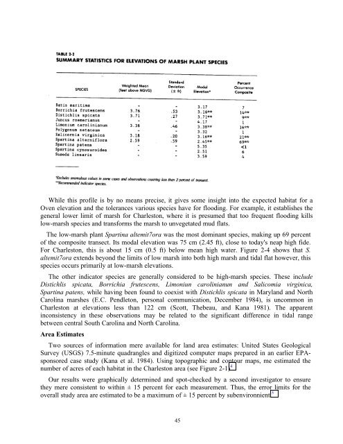
While this profile is by no means precise, it gives some insight into the expected habitat for a
Oven elevation and the tolerances various species have for flooding. For example, it establishes the
general lower limit of marsh for Charleston, where it is presumed that too frequent flooding kills
low-marsh species and transforms the marsh to unvegetated mud flats.
The low-marsh plant Spartina altemit7ora was the most dominant species, making up 69 percent
of the composite transect. Its modal elevation was 75 cm (2.45 ft), close to today's neap high fide.
For Charleston, this is about 15 cm (0.5 ft) below mean high water. Figure 2-4 shows that S.
altemit7ora extends beyond the limits of low marsh into both high marsh and tidal flat however, this
species occurs primarily at low-marsh elevations.
The other indicator species are generally considered to be high-marsh species. These include
Distichlis spicata, Borrichia frutescens, Limoniun carolinianun and Salicomia virginica,
Spartina patens, while having been found to coexist with Distichlis spicata in Maryland and North
Carolina marshes (E.C. Pendleton, personal communication, December 1984), is uncommon in
Charleston at elevations less than 122 cm (Scott, Thebeau, and Kana 1981). The apparent
inconsistency in these observations may be related to the significant difference in tidal range
between central South Carolina and North Carolina.
Area Estimates
Two sources of information mere available for land area estimates: United States Geological
Survey (USGS) 7.5-minute quadrangles and digitized computer maps prepared in an earlier EPAsponsored
case study (Kana et al. 1984). Using topographic and contour maps, me estimated the
number of acres of each habitat in the Charleston area (see Figure 2-1) 4
Our results were graphically determined and spot-checked by a second investigator to ensure
they mere consistent to within ± 15 percent for each measurement. Thus, the error limits for the
overall study area are estimated to be a maximum of ± 15 percent by subenvironnient. 5
45