Elsevier Editorial System(tm) for Hearing Research Manuscript Draft ...
Elsevier Editorial System(tm) for Hearing Research Manuscript Draft ...
Elsevier Editorial System(tm) for Hearing Research Manuscript Draft ...

Create successful ePaper yourself
Turn your PDF publications into a flip-book with our unique Google optimized e-Paper software.
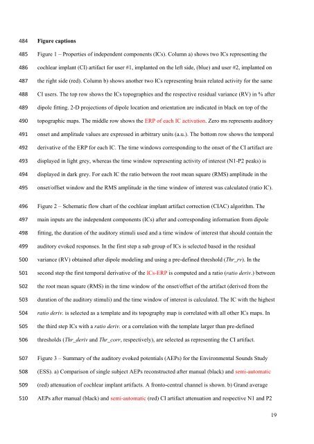
484<br />
485<br />
486<br />
487<br />
488<br />
489<br />
490<br />
491<br />
492<br />
493<br />
494<br />
495<br />
496<br />
497<br />
498<br />
499<br />
500<br />
501<br />
502<br />
503<br />
504<br />
505<br />
506<br />
507<br />
508<br />
509<br />
510<br />
Figure captions<br />
Figure 1 – Properties of independent components (ICs). Column a) shows two ICs representing the<br />
cochlear implant (CI) artifact <strong>for</strong> user #1, implanted on the left side, (blue) and user #2, implanted on<br />
the right side (red). Column b) shows another two ICs representing brain related activity <strong>for</strong> the same<br />
CI users. The top row shows the ICs topographies and the respective residual variance (RV) in % after<br />
dipole fitting. 2-D projections of dipole location and orientation are indicated in black on top of the<br />
topographic maps. The middle row shows the ERP of each IC activation. Zero ms represents auditory<br />
onset and amplitude values are expressed in arbitrary units (a.u.). The bottom row shows the temporal<br />
derivative of the ERP <strong>for</strong> each IC. The time windows corresponding to the onset of the CI artifact are<br />
displayed in light grey, whereas the time window representing activity of interest (N1-P2 peaks) is<br />
displayed in dark grey. For each IC the ratio between the root mean square (RMS) amplitude in the<br />
onset/offset window and the RMS amplitude in the time window of interest was calculated (ratio IC).<br />
Figure 2 – Schematic flow chart of the cochlear implant artifact correction (CIAC) algorithm. The<br />
main inputs are the independent components (ICs) after and corresponding in<strong>for</strong>mation from dipole<br />
fitting, the duration of the auditory stimuli used and a time window of interest that should contain the<br />
auditory evoked responses. In the first step a sub group of ICs is selected based in the residual<br />
variance (RV) obtained after dipole modeling and using a pre-defined threshold (Thr_rv). In the<br />
second step the first temporal derivative of the ICs-ERP is computed and a ratio (ratio deriv.) between<br />
the root mean square (RMS) in the time window of the onset/offset of the artifact (derived from the<br />
duration of the auditory stimuli) and the time window of interest is calculated. The IC with the highest<br />
ratio deriv. is selected as a template and its topography map is correlated with all other ICs maps. In<br />
the third step ICs with a ratio deriv. or a correlation with the template larger than pre-defined<br />
thresholds (Thr_deriv and Thr_corr, respectively), are selected as representing the CI artifact.<br />
Figure 3 – Summary of the auditory evoked potentials (AEPs) <strong>for</strong> the Environmental Sounds Study<br />
(ESS). a) Comparison of single subject AEPs reconstructed after manual (black) and semi-automatic<br />
(red) attenuation of cochlear implant artifacts. A fronto-central channel is shown. b) Grand average<br />
AEPs after manual (black) and semi-automatic (red) CI artifact attenuation and respective N1 and P2<br />
19