A State-Based Programming Model for Wireless Sensor Networks

90 Chapter 5. The Object-State Model
5.4 Parallel Composition
An important element of OSM is the support for parallel state machines. In a
parallel composition of multiple flat state machines, multiple states are active at
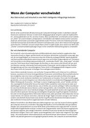
the same time, exactly one for every parallel machine. Let us consider an example
of two parallel state machines, as depicted in Fig. 5.6. (This parallel machine
is the flat state machine from Fig. 5.1 composed in parallel with a copy of the
same machine where state and variable names are primed.) At every discrete
time, this state machine can assume one out of 9 possible state constellations
with two active states each—one for each parallel machine. These constellations
are A|A ′ , A|B ′ , A|C ′ , B|A ′ , B|B and so forth, where A|A ′ is the initial state constellation.
For simplicity we sometimes say A|A ′ is the initial state.
Parallel state machines can handle events originating from independent
sources. For example, independently tracked targets could be handled by parallel
state machines. While events are typically triggered by real-world phenomena
(e.g., a tracked object appears or disappears), events may also be emitted by
the actions of a state machine to support loosely-coupled cooperation of parallel
state machines.
Besides this loose coupling, parallel state machines can be synchronized in the
sense that state transitions of concurrent machines can occur concurrently in the
discrete time model. In the real-time model, however, the state transitions and
associated actions are performed sequentially.
A
outA() inB()
B
outB() inC()
int varA e int varB
f
A’
outA’() inB’()
B’
outB’() inC’()
int varA’ e int varB’
f
C
int varC
C’
int varC’
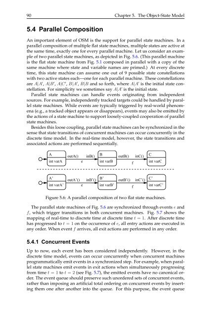
Figure 5.6: A parallel composition of two flat state machines.
The parallel state machines of Fig. 5.6 are synchronized through events e and
f, which trigger transitions in both concurrent machines. Fig. 5.7 shows the
mapping of real-time to discrete time at discrete time t = 1. After discrete time
has progressed to t = 1 on the occurrence of e, all entry actions are executed in
any order. When event f arrives, all exit actions are performed in any order.
5.4.1 Concurrent Events
Up to now, each event has been considered independently. However, in the
discrete time model, events can occur concurrently when concurrent machines
programmatically emit events in a synchronized step. For example, when parallel
state machines emit events in exit actions when simultaneously progressing
from time t = 1 to t = 2 (see Fig. 5.7), the emitted events have no canonical order.
The event queue should preserve such unordered sets of concurrent events,
rather than imposing an artificial total ordering on concurrent events by inserting
them one after another into the queue. For this purpose, the event queue