Answers to Selected Problems

Its necessary condition to maximize profit is that
price equals marginal cost: p - dC(q)/dq = 0.
Industry supply is determined by entry, which occurs
until profits are driven to zero (we ignore the problem
of fractional firms and treat the number of firms, n,
as a continuous variable): pq - [C(q) + l] = 0. In
equilibrium, each firm produces the same output, q,
so market output is Q = nq, and the market inverse
demand function is p = p(Q) = p(nq). By substituting
the market inverse demand function into the
necessary and sufficient condition, we determine the
market equilibrium (n*, q*) by the two conditions:
p(n*q*) - dC(q*)/dq = 0,
p(n*q*)q* - [C(q*) + l] = 0.
For notational simplicity, we henceforth leave
off the asterisks. To determine how the equilibrium
is affected by an increase in the lump-sum tax,
we evaluate the comparative statics at l = 0. We
totally differentiate our two equilibrium equations
with respect to the two endogenous variables, n and
q, and the exogenous variable, l:
dq(n[dp(nq)/dQ] - d2C(q)/dq2 )
+ dn(q[dp(nq)/dQ]) + dl (0) = 0,
dq(n[qdp(nq)/dQ] + p(nq) - dC/dq)
+ dn(q2 [dp(nq)/dQ]) - dl = 0.
We can write these equations in matrix form (noting
that p - dC/dq = 0 from the necessary condition) as
n
4
dp
dQ - d2C dq2 nq dp
dQ
q dp
dQ
dp
q2 dQ
4 J dq
R = J0
dn 1 Rdl.
There are several ways to solve these equations.
One is to use Cramer’s rule. Define
n
D = 4
dp
dQ - d2C dq2 nq dp
dQ
q dp
dQ
4
dp
q2 dQ
= ¢n dp
dQ - d2C dp
≤q2
dq2 dQ
= - d2C dp
q2 7 0,
dq2 dQ
dp dp
- q ¢nq
dQ dQ ≤
where the inequality follows from each firm’s sufficient
condition. Using Cramer’s rule:
dq
dl =
0 q
4
dp
dQ
4
dp
2 1 q
dQ
=
D
-q dp
dQ
D
7 0,
dn
dl =
Answers to Selected Problems
n
4
dp
dQ - d2C dq2 nq dp
dQ
D
The change in price is
dp(nq)
dl
Chapter 9
0
4
1
=
dp dn dq
= Jq + n
dQ dl dl R
= dp
dQ D
¢n dp
dQ - d2C dq
D
= dp
dQ §
- d2C q
2 dq
D
n dp
dQ - d2 C
dq 2
2 ≤q
¥ 7 0.
D
-
E-41
6 0.
nq dp
dQ
D T
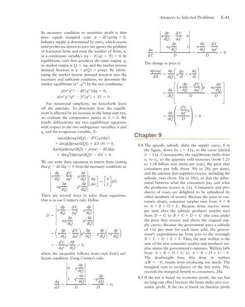
5.5 The specific subsidy shifts the supply curve, S in
the figure, down by s = 11., to the curve labeled
S - 11.. Consequently, the equilibrium shifts from
e1 to e2 , so the quantity sold increases (from 1.25
to 1.34 billion rose stems per year), the price that
consumers pay falls (from 30¢ to 28¢ per stem),
and the amount that suppliers receive, including the
subsidy, rises (from 30¢ to 39¢), so that the differential
between what the consumers pay and what
the producers receive is 11¢. Consumers and producers
of roses are delighted to be subsidized by
other members of society. Because the price to customers
drops, consumer surplus rises from A + B
to A + B + D + E. Because firms receive more
per stem after the subsidy, producer surplus rises
from D + G to B + C + D + G (the area under
the price they receive and above the original supply
curve). Because the government pays a subsidy
of 11¢ per stem for each stem sold, the government’s
expenditures go from zero to the rectangle
B + C + D + E + F. Thus, the new welfare is the
sum of the new consumer surplus and producer surplus
minus the government’s expenses. Welfare falls
from A + B + D + G to A + B + D + G - F.
The deadweight loss, this drop in welfare
∆W = -F, results from producing too much: The
marginal cost to producers of the last stem, 39¢,
exceeds the marginal benefit to consumers, 28¢.
5.7 If the tax is based on economic profit, the tax has
no long-run effect because the firms make zero economic
profit. If the tax is based on business profit